Quark confinement due to unified magnetic monopoles and vortices reduced from symmetric instantons with holography
January 05, 2026
1 Introduction↩︎
Quark confinement means that quarks as the most fundamental building blocks of the matter have never been observed in the isolated form and must be confined in hadrons. This is caused by strong interactions mediated by
gluons which are described by the Yang-Mills theory, i.e., the non-Abelian gauge theory. In this talk we consider quark confinement in the 4-dim. (\(D=4\)) quantum Yang-Mills theory
according to the Wilson criterion (with no dynamical quarks):
area law of the Wilson loop average \(\Leftrightarrow\) linear potential for static \(q\bar{q}\) potential.
Quark confinement in this sense can be understood based on the dual superconductor picture proposed by Nambu, ’t Hooft, Mandelstam, Polyakov in the mid-1970s. For this purpose, we need magnetic monopoles and/or vortices. For a review, see e.g., Kondo et al.[1]. Nevertheless, topological solitons in Yang-Mills theory are only instantons in the \(D=4\) Euclidean space \(\mathbb{R}^4\). It is a big question how to derive such lower-dim. topological objects from the \(D=4\) Yang-Mills theory.
The topological solitons in the Yang-Mills theory are only instantons in 4-dim. Euclidean spacetime \(\mathbb{R}^4\). [Coleman-Deser-Pagels theorem] It is known that various low-dimensional integrable equations can be obtained from the self-dual Yang-Mills equations in 4-dim. space \(\mathbb{R}^4\) by dimensional reduction.
The \(D=4\) Yang-Mills theory has conformal symmetry. The self-dual Yang-Mills equation on \(\mathbb{R}^4\) has also the conformal symmetry, whose solutions (instantons)
give solutions of the Yang-Mills field equation with a finite Euclidean action. Therefore, we consider the Yang-Mills theory on the 4-dim. Euclidean spacetime \(\mathbb{R}^4(x^1,x^2,x^3,x^4)\). In this talk we show that
\(D=3\) magnetic monopoles and \(D=2\) (center) vortices responsible for quark confinement are constructed from symmetric instantons in the \(D=4\)
Euclidean Yang-Mills theory in a way consistent with holography principle. This result is obtained [2] based on the guiding
principles:
\(\bullet\) conformal equivalence: conformal symmetry,
\(\bullet\) symmetric instanton gauge field: spatial symmetry \(SO(2)\), \(SO(3)\),
\(\bullet\) dimensional reductions: self-dual equation (electric-magnetic dual symmetry).
2 Translation symmetry and dimensional reduction↩︎
We consider \(SU(2)\) Yang-Mills theory on the \(D=4\) Euclidean space \(\mathbb{R}^4(x^1,x^2,x^3,{t})\). The Euclidean time \(x^4\) is written as \(t\) in what follows. For the Yang-Mills field \(\mathscr{A}_\mu(x) := \mathscr{A}_\mu^A(x) \frac{\sigma_A}{2}\) with the Pauli matrices \(\sigma_A (A=1,2,3)\), the action is given by \[\begin{align} S_{\rm{E}}^{\rm{YM}} =& \int d^4 x~\mathscr{L}_{\rm{E}}^{\rm{YM}} = \int d^4 x \frac{1}{2} {\rm tr}(\mathscr{F}_{\mu\nu}(x) \mathscr{F}_{\mu\nu}(x)) = \int d^4 x~\frac{1}{4}\mathscr{F}_{\mu\nu}^A(x) \mathscr{F}_{\mu\nu}^A(x) , \nonumber\\ \mathscr{F}_{\mu\nu}(x) :=& \partial_\mu \mathscr{A}_\nu(x) - \partial_\nu \mathscr{A}_\mu(x) - ig [\mathscr{A}_\mu(x), \mathscr{A}_\nu(x)] = \mathscr{F}_{\mu\nu}^A(x) \frac{\sigma_A}{2} \in su(2). \end{align}\] In what follows use \(g\) for the gauge coupling constant \(g_{{}_{\rm YM}}\) to simplify the notation. The the metric is given by \[(ds)^2(\mathbb{R}^4) = [(dx^1)^2 + (dx^2)^2 + (dx^3)^2] + (d{t})^2 \Longrightarrow \mathbb{R}^4 = \mathbb{R}^3 \times \mathbb{R}^1 .\] The self-dual Yang-Mills equation is given by \[\begin{align} *\mathscr{F}_{\mu\nu}(\boldsymbol{x},t) := \frac{1}{2} \epsilon_{\alpha\beta\mu\nu} \mathscr{F}_{\alpha\beta}(\boldsymbol{x},t) = \mathscr{F}_{\mu\nu}(\boldsymbol{x},t) \;[x = (x^1,x^2,x^3,{t})=(\boldsymbol{x},t) \in \mathbb{R}^4 ]. \label{SD-YMeq} \end{align}\tag{1}\]
(0) First, we consider a solution for the gauge field that has the translation symmetry in the time \(\textcolor{red}{t={x^4}}\), which is equivalent to the \(t\)-independence: \[\begin{align} (\mathscr{A}_{1}(\boldsymbol{x},t), \mathscr{A}_{2}(\boldsymbol{x},t), \mathscr{A}_{3}(\boldsymbol{x},t), \mathscr{A}_{t}(\boldsymbol{x},t)) \to (\mathscr{A}_{1}(\boldsymbol{x}), \mathscr{A}_{2}(\boldsymbol{x}), \mathscr{A}_{3}(\boldsymbol{x}), \Phi(\boldsymbol{x})) . \end{align}\] The time-independent solution of the self-dual equation (1 ) reduces to the solution of Bogomolny equation on \(\mathbb{R}^3\): \[\begin{align} (*\mathscr{F})_{\ell t}(\boldsymbol{x}) = \mathscr{D}_\ell \Phi(\boldsymbol{x}), \;\ell=1,2,3, \quad \boldsymbol{x} := (x^1,x^2,x^3) \in \mathbb{R}^3 . \end{align}\] In fact, the self-dual equation for \(\mu, \nu=\ell , t\) reads for \(\Phi(\boldsymbol{x}) := \mathscr{A}_{t}(\boldsymbol{x})\) \[\begin{align} \pm \frac{1}{2} \epsilon_{jk\ell t} \mathscr{F}_{jk}(\boldsymbol{x}) =\mathscr{F}_{\ell t}(\boldsymbol{x}) =& \partial_\ell \mathscr{A}_t(\boldsymbol{x}) - {\partial_{t}} \mathscr{A}_\ell (\boldsymbol{x}) -ig[ \mathscr{A}_\ell (\boldsymbol{x}), \mathscr{A}_t(\boldsymbol{x})] \;( {\partial_{t}} \mathscr{A}_\ell (x^1,x^2,x^3)=0) \nonumber\\ =& \partial_\ell \mathscr{A}_t(\boldsymbol{x}) -ig[ \mathscr{A}_\ell (\boldsymbol{x}), \mathscr{A}_t(\boldsymbol{x})] = \mathscr{D}_\ell \Phi(\boldsymbol{x}) . \end{align}\] The solution of the Bogomolny equation is called the Prasad-Sommerfield (PS) magnetic monopole. However, this solution leads to a divergent 4-dim. action: \[S=\int_{-\infty}^{\infty}d{t} \left[ \int dx^1 dx^2 dx^3 \mathscr{L}(x^1,x^2,x^3)\right] =\infty \Longrightarrow \exp( -S/\hbar) =0 ,\] even if \(\int dx^1 dx^2 dx^3 \mathscr{L}(x^1,x^2,x^3)<\infty\) because of the \(t\)-independence.
Therefore, the PS magnetic monopole does not contribute to the path integral. Thus, the PS magnetic monopole is not responsible for quark confinement. How to avoid this difficulty?
3 Conformal equivalence (I)↩︎
(I) Next, we consider solutions with spatial rotation symmetry: \(SO(2) \simeq S^1\).
In \(\mathbb{R}^4\) with the metric \((ds)^2(\mathbb{R}^4)
= (dx^1)^2 + (dx^2)^2 + (dx^3)^2 + (d{t})^2\), we introduce the coordinates \((\rho,\varphi)\) in the 2-dim. space \((x^1,x^2)\) to rewrite the metric:\[\begin{align}
(ds)^2(\mathbb{R}^4)
= (d\rho)^2 + \rho^2(d\varphi)^2 + (dx^3)^2 + (d{t})^2 ,
\end{align}\] where \(\rho := \sqrt{(x^1)^2 + (x^2)^2}\). We factor out \(\rho^2\) as a conformal factor to further rewrite the metric: \[\begin{align}
(ds)^2(\mathbb{R}^4) = \rho^2\Big[\frac{(dx^3)^2 + (d{t})^2 + (d\rho)^2}{\rho^2} + (d\varphi)^2\Big].
\end{align}\] Therefore, we obtain a conformal equivalence: See the left panel of Fig.1. \[\begin{array}{cccccccc}
\mathbb{R}^4 = \mathbb{R}^3 \times \mathbb{R}^1\rightarrow&\mathbb{R}^4 &\backslash& \mathbb{R}^2 &\simeq& \mathbb{H}^3& \times &S^1\\
&\rotatebox{90}{\in}&&\rotatebox{90}{\in}&&\rotatebox{90}{\in}&&\rotatebox{90}{\in}\\
&(x^1,x^2,x^3,{t})&&(x^3,{t})&&(\rho,x^3,{t})&&\varphi
\end{array}\] \(\mathbb{H}^3(\rho,x^3,{t})\) is a hyperbolic 3-space: \(x^3,{t} \in (-\infty,+\infty)\), \(\rho \in (0,\infty)\), and
has the metric \(g_{\mu\nu}=\rho^{-2}\delta_{\mu\nu}\) with the negative constant curvature \(-1\). This is the upper half space model with \(\rho>0\). Here \(\rho = 0\) is a singularity, therefore the corresponding 2-dim. space, i.e., the \((x^3,{t})\) plane with \(\rho =
0\) must be excluded from \(\mathbb{R}^4\). While \(S^1(\varphi)\) is a 1-dimensional unit sphere, i.e., a unit circle with the coordinate \(\varphi \in
[0,2\pi)\). Here \(SO(2)\) acts on \(S^1(\varphi)\) in the standard way. See the left panel of Fig. 1.
The \(SO(2) \simeq S^1\) symmetric instanton solution on \(\mathbb{R}^4 \backslash \mathbb{R}^2\) that does not depend on the rotation angle \(\varphi\) reduces to the hyperbolic magnetic monopole solution on \(\mathbb{H}^3\): the \(\varphi\)-rotation symmetry = \(\varphi\)-independence as the dimensional reduction: \[\begin{align} x=(x^1,x^2,x^3,{t}) \equiv (\rho,{\varphi},x^3,{t}) \to (\rho,x^3,{t}) , \end{align}\] which is associated with the field identification \(\Phi(\rho,x^3,{t}) := \mathscr{A}_\varphi(\rho,x^3,{t})\): \[\begin{align} & (\mathscr{A}_{\rho}(\rho,\varphi,x^3,t), {\mathscr{A}_{\varphi}}(\rho,\varphi,x^3,t), \mathscr{A}_{3}(\rho,\varphi,x^3,t), \mathscr{A}_{4}(\rho,\varphi,x^3,t)) \nonumber\\ \to & (\mathscr{A}_{\rho}(\rho,x^3,{t}), {\Phi}(\rho,x^3,{t}), \mathscr{A}_{3}(\rho,x^3,{t}), \mathscr{A}_{4}(\rho,x^3,{t})), \;(\rho,x^3,{t}) \in \mathbb{H}^3 . \end{align}\]
Any solution of the Bogomolny equation on \(\mathbb{H}^3\) is a \(\varphi\)-independent instanton solution of the self-dual equation on \(\mathbb{R}^4 \backslash \mathbb{R}^2\), (\({\partial_\varphi} \mathscr{A}_\ell (\rho,x^3,{t})=0\)): \[\begin{align} (*\mathscr{F})_{\ell \varphi}(\rho,x^3,{t}) =& \frac{1}{\rho} \mathscr{D}_\ell \Phi(\rho,x^3,{t}), \;(\rho,x^3,{t}) \in \mathbb{H}^3 . \end{align}\] Since \(S^1\) is compact (unlike \(\mathbb{R}^1\)), any solution of the Bogomolny equation giving a finite 3-dim. action on \(\mathbb{H}^3\) gives a configuration with a finite 4-dim. action: \[S= \int_{0}^{2\pi}d\varphi \left[ \int_{0}^{\infty}d\rho \;\rho \int_{-\infty}^{\infty}dx^3 \int_{-\infty}^{\infty}d{t} \mathscr{L}(\rho,x^3,{t}) \right] <\infty .\] Therefore, \(S^1\simeq SO(2)\) symmetric instantons on \(\mathbb{R}^4\) can be reinterpreted as hyperbolic magnetic monopoles on \(\mathbb{H}^3\), giving a configuration with a finite 4-dim. action. This case (I) was first pointed out by Atiyah (1984)[3]. Therefore, the hyperbolic magnetic monopoles can contribute to the path integral, because \[\exp( -S/\hbar) \not= 0 .\] Thus, the hyperbolic magnetic monopoles can be responsible for quark confinement.
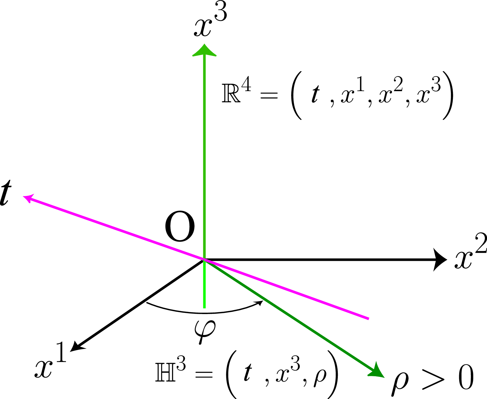
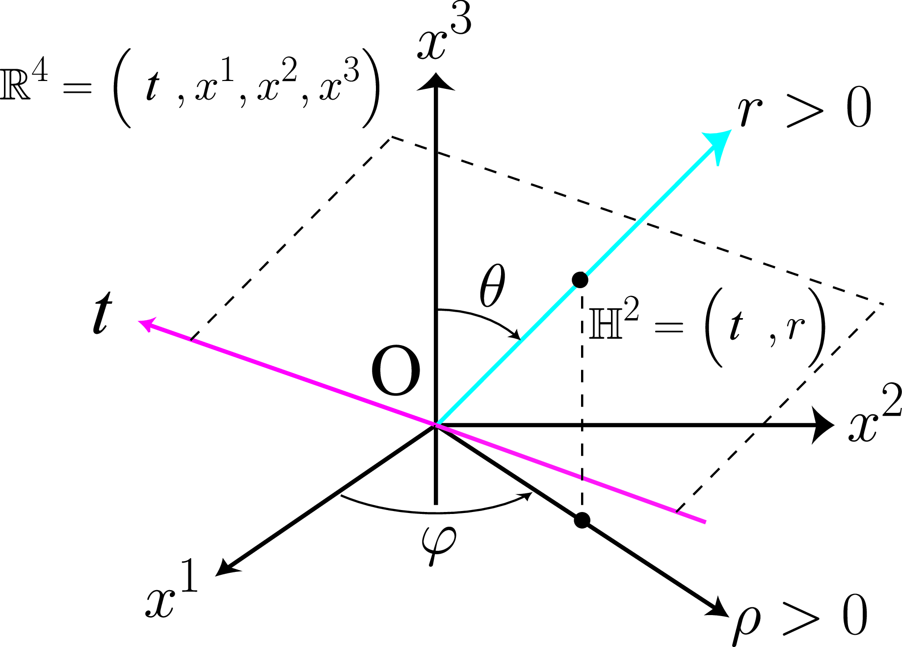
Figure 1: Conformal equivalence and symmetry reduction: (Left) 4-dim. Euclidean space \(\mathbb{R}^4({t},x^1,x^2,x^3)\) versus 3-dim. hyperbolic space \(\mathbb{H}^3({t},x^3,\rho)\).
(Right) 4-dim. Euclidean space \(\mathbb{R}^4({t},x^1,x^2,x^3)\) versus 2-dim. hyperbolic space \(\mathbb{H}^2({t},r)\)..
4 Conformal equivalence (II)↩︎
(II) We consider another solution with spatial rotation symmetry: \(SO(3)\).
We introduce the polar coordinates \((r,\theta,\varphi)\) for the 3-dim. space \((x^1,x^2,x^3)\): \[\begin{align}
(ds)^2(\mathbb{R}^4) = (d{t})^2 + (dr)^2 +r^2((d\theta)^2 +\sin^2\theta(d\varphi)^2) ,
\end{align}\] where \(r := \sqrt{(x^1)^2 + (x^2)^2 + (x^3)^2}\). Then, we factor out \(r^2\) as a conformal factor to rewrite \[(ds)^2(\mathbb{R}^4) =r^2 \Big[ \frac{(d{t})^2 + (dr)^2}{r^2} +((d\theta)^2 +\sin^2\theta(d\varphi)^2) \Big].\] Therefore, we obtain the conformal equivalence: See the right panel of Fig.1.\[\begin{align}
\begin{array}{cccccccc}
\mathbb{R}^4 = \mathbb{R}^2 \times \mathbb{R}^2\rightarrow&\mathbb{R}^4 &\backslash& \mathbb{R}^1 &\simeq& \mathbb{H}^2&\times &S^2\\
&\rotatebox{90}{\in}&&\rotatebox{90}{\in}&&\rotatebox{90}{\in}&&\rotatebox{90}{\in}\\
&(t,x,y,z)&&t&&(t,r)&&(\theta,\varphi)
\end{array}
\end{align}\]
\(\mathbb{H}^2({t},r)\) is a hyperbolic plane with \({t} \in (-\infty,\infty)\), \(r \in(0,\infty)\), and has the metric \(g_{\mu\nu}=r^{-2}\delta_{\mu\nu}\) with the negative constant curvature \((-1)\). This is the upper half plane model with \(r >0\). Here \(r=0\) is a singularity: the \({t}\)-axis must be excluded from \(\mathbb{R}^4\). While \(S^2(\theta,\varphi)\) is a two-dimensional unit sphere with \(\theta \in [0,\pi)\), \(\varphi \in [0,2\pi)\) and has a positive constant curvature (2). \(SO(3)\) acts on \(S^2(\theta,\varphi)\) in the standard way. The \(SO(3)\) (spherically) symmetric instanton on \(\mathbb{R}^4 \backslash \mathbb{R}^1\) that does not depend on the rotation angles \(\theta,\varphi\) reduces to hyperbolic vortex on \(\mathbb{H}^2(r,{t})\). See the right panel of Fig. 1.
Any solution of the vortex equation on \(\mathbb{H}^2(r,{t})\) is a \(\theta,\varphi\)-independent solution of self-dual equation on \(\mathbb{R}^4 \backslash \mathbb{R}^1\) which is written for \(a_t=a_t(r,{t}) , a_r=a_r(r,{t}) , \;\phi_1=\phi_1(r,{t}) , \;\phi_2=\phi_2(r,{t}), \;(r,{t}) \in \mathbb{H}^2\): \[\begin{align} \left\{\, \begin{aligned} & \partial_{t}a_r - \partial_ra_t = \frac{1}{r^2}(1 - \phi_1^2 - \phi_2^2), \\ &\partial_{t}\phi_1 + a_t\phi_2 = \partial_r\phi_2 - a_r\phi_1, \; \partial_{t}\phi_2 - a_t\phi_1 = -(\partial_r\phi_1 + a_r\phi_2) . \end{aligned} \right. \end{align}\] Any solution of the vortex equation giving a finite 2-dim. action on \(\mathbb{H}^2(r,{t})\) \(\int_{0}^{\infty}dr \;r^2 \int_{-\infty}^{\infty}d{t} \mathscr{L}(r,{t}) <\infty\) gives a finite 4-dim. action: \(S= \int_{0}^{\pi}d\theta \sin \theta \int_{0}^{2\pi}d\varphi \left[ \int_{0}^{\infty}dr \;r^2 \int_{-\infty}^{\infty}d{t} \mathscr{L}(r,{t}) \right] <\infty ,\) since \(S^2(\theta,\varphi)\) is compact.
Therefore, \(SO(3)\) spherically symmetric instantons on \(\mathbb{R}^4\) can be reinterpreted as vortices on \(\mathbb{H}^2\), giving a configuration with a finite 4-dim. action. This case (II) was discovered by Witten (1977)[4]. to find multi-instanton solutions of 4-dim. Yang-Mills theory, which is established as the symmetric instanton by Forgacs and Manton (1980)[5]. Therefore, the hyperbolic vortices can contribute to the path integral due to \(\exp( -S/\hbar) \not= 0\) and the hyperbolic vortices can be responsible for quark confinement.
The results (I), (II) are summarized in Fig. 2. Conformal equivalence reshapes the background geometry, while symmetry reduction eliminates dependence of field content on compact directions. The crucial point is that translation-invariant monopoles in flat \(\mathbb{R}\) have infinite four-dimensional action, whereas rotation-invariant instantons effectively compactify the reduced directions, rendering the action finite. In the semi-classical regime, these finite-action configurations dominate the infrared path integral and thus control the Wilson loop behavior.
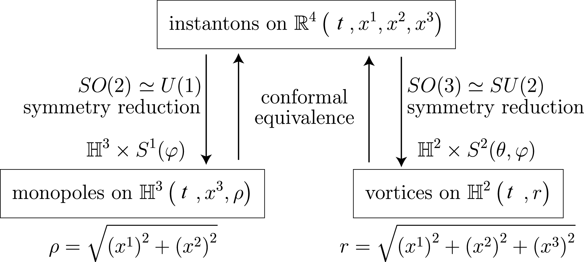
Figure 2: Symmetric instanton, conformal equivalence, and dimensional reduction..
5 Unifying magnetic monopole and vortices↩︎
Definition [Rotationally symmetric gauge field](Manton and Sutcliffe(2004)[6])
If the space rotation \(R\) has the same effect on the gauge field as the gauge transformation \(U_R\): \[\begin{align}
R_{kj}\mathscr{A}_k(R\boldsymbol{x}) =& U_R(\boldsymbol{x})\mathscr{A}_j(\boldsymbol{x})U_R^{-1}(\boldsymbol{x}) + iU_R(\boldsymbol{x})\partial_jU_R^{-1}(\boldsymbol{x}) ,
\end{align}\] the gauge field \(\mathscr{A}(x)\) is called rotationally symmetric. Or equivalently, if we combine \(R\) and \(U_R^{-1}\), the
gauge field remains invariant.
Proposition[Witten transformation (Witten Ansatz) for \(SO(3)\) symmetric gauge field]
The \(D=4\) \(SU(2)\) Yang-Mills field \(\mathscr{A}_\mu(x)\) with \(SO(3)\) spatial rotation symmetry on \(\mathbb{R}^4(x)\) is dimensionally reduced to the \(D=2\) gauge field \(a_t(r,{t}), a_r(r,{t})\) and the scalar field \(\phi_1(r,{t}),
\phi_2(r,{t})\) on \(\mathbb{H}^2(t,r)\) through the transformation which we call the Witten transformation (called the Witten Ansatz): \[\begin{align}
\mathscr{A}_{t}(x) = \frac{\sigma_A}{2}\frac{x^A}{r}a_t(r,{t}) , \quad
\mathscr{A}_j(x) =\frac{\sigma_A}{2}\left\{\frac{x^A}{r}\frac{x^j}{r}a_r(r,{t}) + \frac{\delta_j^Ar^2 - x^Ax^j}{r^3}\phi_1(r,{t}) + \epsilon_{jAk}\frac{x^k}{r^2}[1 + \phi_2(r,{t})]\right\}.
\end{align}\]
Proposition [magnetic monopole on \(\mathbb{H}^3\), vortex on \(\mathbb{H}^2\)] We can apply the gauge transformation \[U_\varphi=\exp \left( i\varphi\frac{\sigma_3}{2} \right) \in SU(2) \;\left( \varphi:=\arctan \frac{x^2}{x^1} \in [0, 2\pi) \right)\] corresponding to a rotation around the \(x_3\) axis by an angle \(\varphi\) to the instanton: \[\begin{align} \mathscr{A}_\mu(x^1,x^2, x^3,{t}) \rightarrow U_\varphi \mathscr{A}_\mu(x^1,x^2, x^3,{t}) U_\varphi^\dagger + iU_\varphi\partial_\mu U_\varphi^\dagger =: \mathscr{A}_\mu^G(\rho, x^3,{t}) . \end{align}\] so that \(\mathscr{A}_\mu(x^1,x^2,x^3,{t})\) becomes independent of \(\varphi\), leading to an \(S^1\)-symmetric instanton \(\mathscr{A}_\mu^G(\rho,x^3,{t})\). Then the magnetic monopole on \(\mathbb{H}^3(\rho,x^3,{t})\) is written in terms of the vortex on \(\mathbb{H}^2(r,{t})\): \[\begin{align} \mathscr{A}_t^G(\rho, x^3,{t}) =&\frac{1}{2}\left\{\frac{1}{r}(\sigma_1\rho + \sigma_3x_3)\right\}a_t(r,{t}), \nonumber \\ \mathscr{A}_3^G(\rho, x^3,{t}) =&\frac{1}{2}\left\{\frac{x^3}{r^2}(\sigma_1\rho + \sigma_3x^3)a_r(r,{t}) + \frac{\rho}{r^3}(-\sigma_1x^3 +\sigma_3\rho)\phi_1(r,{t}) - \frac{\rho}{r^2}\sigma_2(1 + \phi_2(r,{t}))\right\}, \nonumber \\ \mathscr{A}_\rho^G(\rho, x^3,{t}) =&\frac{1}{2}\left\{\frac{\rho}{r^2}(\sigma_1\rho + \sigma_3x^3)a_r(r,{t}) + \frac{x^3}{r^3}(\sigma_1x^3 -\sigma_3\rho)\phi_1(r,{t}) + \frac{x^3}{r^2}\sigma_2(1 + \phi_2(r,{t}))\right\}, \nonumber \\ \Phi(\rho, x^3,{t}) =& \frac{1}{2}\left\{\frac{\rho}{r}\sigma_2\phi_1(r,{t}) + \frac{\rho}{r^2}(-\sigma_1x^3 +\sigma_3\rho)(1 + \phi_2(r,{t})) +\sigma_3\right\}. \end{align}\] Although this result was obtained by Maldonado (2017)[7], it is modified for our later convenience. Equation (24) provides a non-trivial explicit map between monopole and vortex fields, going beyond qualitative correspondence. The relationship for the norm between the \(su(2)\)-valued hyperbolic magnetic monopole field \(\Phi(\rho, x^3,{t})=\mathscr{A}_\varphi^G(\rho, x^3,{t})\) and the complex-valued hyperbolic vortex field \(\phi({t},r)=\phi_1({t},r)+i\phi_2({t},r)\) is given as \[\begin{align} ||\Phi({t},x^3,\rho)||^2 = \frac{\rho^2|\phi({t},r)|^2 + (x^3)^2}{tr^2} , \quad r:=\sqrt{\rho^2 + (x^3)^2} . \end{align}\] The norm \(||\Phi||\) has the correct boundary value: \(||\Phi|| \rightarrow v = \frac{1}{2}\) \((\rho\rightarrow0)\).
6 Holography: bulk/boundary correspondence↩︎
It was rigorously shown that the holographic principle applies to hyperbolic magnetic monopoles in the hyperbolic space \(\mathbb{H}^3\). In contrast, it does not apply to magnetic
monopoles in flat Euclidean space \(\mathbb{R}^3\). See references in [2]. Here ‘holography’ means the uniqueness
of hyperbolic monopole solutions given their asymptotic boundary data, modulo gauge equivalence.
Proposition [Bulk/boundary correspondence of \(\mathbb{H}^3=AdS_3\)] A magnetic monopole on hyperbolic space (anti-de Sitter space) \(\mathbb{H}^3=AdS_3\) is completely
determined by its asymptotic boundary value at infinity \(\partial\mathbb{H}^3\), apart from the gauge equivalence. This situation is in sharp contrast with the Euclidean case in which all monopole have the same boundary
values.
Proposition [Abelian dominance and magnetic monopole dominance on \(\partial\mathbb{H}^3\)] On the conformal boundary \(\partial\mathbb{H}^3 \simeq S^2\) of \(\mathbb{H}^3(\rho,x^3,{t})\), that is, \(\rho \to 0\): \({t}\)-\(x^3\) plane, the \(SU(2)\) Yang-Mills field and the \(SU(2)\) scalar field converges to \[\begin{align} \mathscr{A}_{t}^G(\rho,x^3,{t}) &\to \frac{{\sigma_3}}{2}a_t({t},x^3) , \;\mathscr{A}_3^G(\rho,x^3,{t}) \to \frac{{\sigma_3}}{2}a_r({t},x^3) , \nonumber\\ \mathscr{A}_\rho^G(\rho,x^3,{t}) &\to \frac{{\sigma_1}}{2}\frac{1}{r}\phi_1({t},x^3) + \frac{{\sigma_2}}{2}\frac{1}{r} [1 + \phi_2({t},x^3)], \nonumber\\ \Phi(\rho,x^3,{t}) &\to \frac{{\sigma_3}}{2}(1) \;\left( ||\Phi || \to v=\frac{1}{2} \right) . \end{align}\] Therefore, the gauge field \(\mathscr{A}_\rho^G(\rho,x^3,{t})\) in the bulk direction is dominated by the off-diagonal components, while the gauge field \(\mathscr{A}_4^G(\rho,x^3,{t}), \mathscr{A}_3^G(\rho,x^3,{t})\) on the boundary \(\rho=0\) has only the diagonal components \(a_t({t},x^3), a_r({t},x^3)\).
7 Quark confinement: area law of Wilson loop average↩︎
Definition [Wilson loop operator] Let \(\mathscr{A}\) be a Lie algebra valued connection 1-form: \[\mathscr{A}(x) := \mathscr{A}_\mu(x) dx^\mu = \mathscr{A}_\mu^A(x) T_A dx^\mu.\] For a given loop \(C\), the Wilson loop operator \(W_{\rm C}[\mathscr{A}]\) in the representation \(\mathcal{R}\) is defined using the path ordered product \(\mathscr{P}\): \[W_C[\mathscr{A}] := {\rm tr}_{\mathcal{R}} \left\{ \mathscr{P} \exp \left[ ig \oint_C \mathscr{A} \right] \right\} /{\rm tr}_{\mathcal{R}}(1).\]
(I) Quark confinement due to hyperbolic magnetic monopoles on \(\mathbb{H}^3\) and holography: We locate the Wilson loop \(C\) on the boundary \(\partial\mathbb{H}^3(x^3,{t})\) of \(\mathbb{H}^3\) in the limit \(\rho \to 0\). See the left panel of Fig. 3.
Proposition [Wilson loop operator on the conformal boundary \(\partial \mathbb{H}^3\)] If the loop \(C\) lies on the conformal boundary \(\partial \mathbb{H}^3\), i.e., \(x^3-{t}\) of \(\mathbb{H}^3\), the Wilson loop operator in the fundamental representation \(F\) defined for the \(S^1\)-invariant \(SU(2)\) Yang-Mills field \(\mathscr{A}_\mu^G\) takes the simple Abelian form as \(\rho \to 0\): \[\begin{align} W_C[\mathscr{A}] = \frac{1}{2} {\rm tr}_{F} \left\{ \exp \left[ i \frac{\sigma_3}{2} \oint_C dx^\mu a_\mu({t},x^3) \right] \right\} = \frac{1}{2} {\rm tr}_{F} \left\{ \exp \left[ i \frac{\sigma_3}{2} \int_{\Sigma: \partial \Sigma=C} dt dx^3 F_{tr}({t},x^3) \right] \right\} . \end{align}\] The \(SU(2)\) field strength on the boundary has only the maximal torus \(U(1)\) component: \[\begin{align} \mathscr{F}_{t3}^G(\rho,x^3,{t}) \to \frac{\sigma_3}{2}(\partial_{t}a_r - \partial_ra_t) =\frac{\sigma_3}{2} F_{tr}({t},x^3). \end{align}\] Therefore, the Yang-Mills field reduces to the diagonal Abelian field on the conformal boundary \(x^3-{t}\). This fact is regarded as the (infrared) Abelian dominance and the magnetic monopole dominance in quark confinement. In the ordinary flat Euclidean case, (infrared) Abelian dominance and magnetic monopole dominance in quark confinement have been confirmed by numerical simulations and also supported by analytical investigations, but not proved rigorously in the Euclidean case. See e.g., [1].
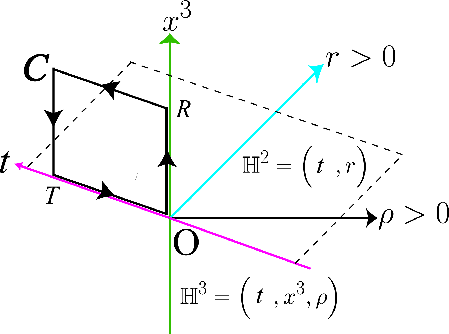
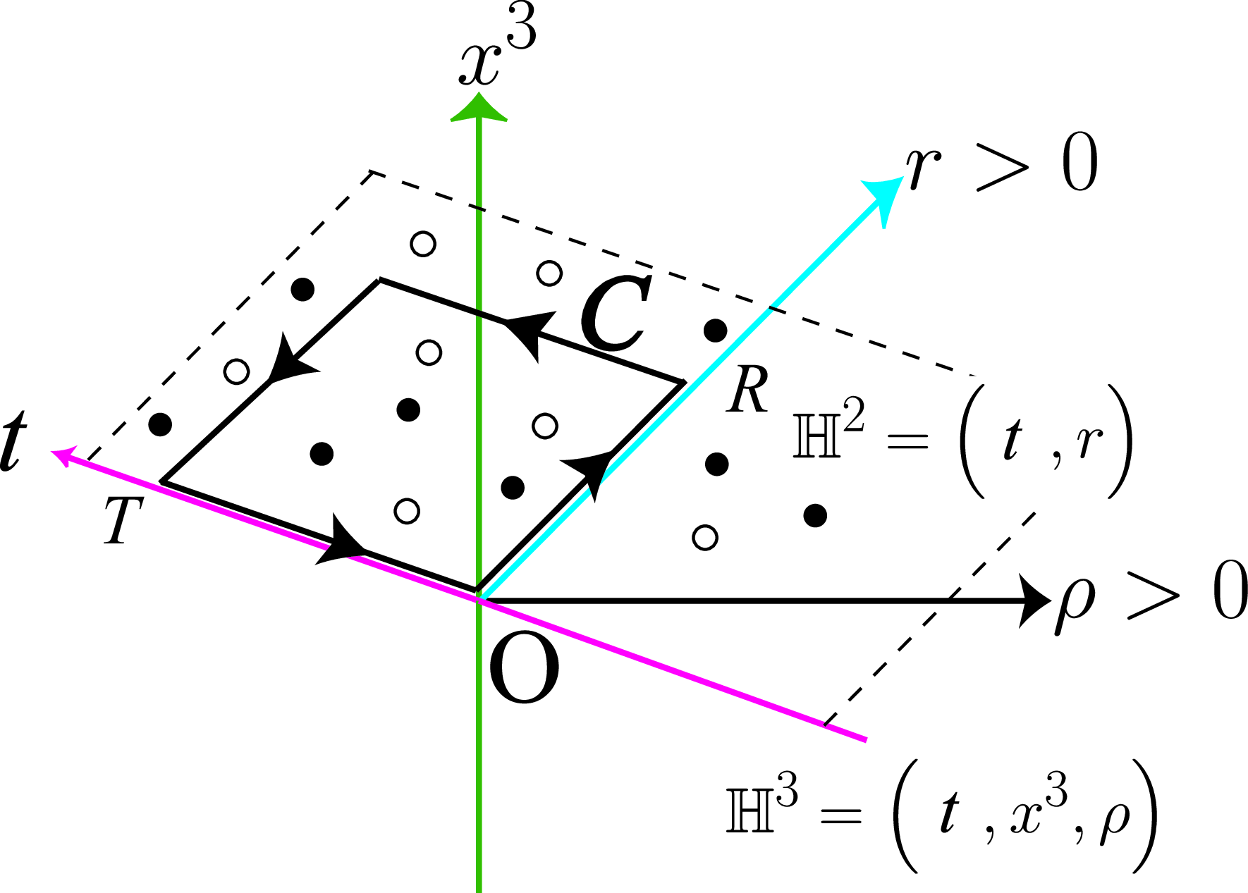
Figure 3: (Left) The Wilson loop \(C\) located on the conformal boundary \(\partial \mathbb{H}^3\), i.e., \(t-x^3\) plane of the hyperbolic space \(\mathbb{H}^3\). (Right) The Wilson loop \(C\) located on \(\partial \mathbb{H}^2\), i.e., \(t-r\) plane of the hyperbolic plane \(\mathbb{H}^2\). Hyperbolic vortices (black circles) and anti-vortices (white circles) located inside and outside of the Wilson loop \(C\) on \(\mathbb{H}^2\)..
(II) Quark confinement due to hyperbolic vortices on \(\mathbb{H}^2\): See the right panel of Fig. 3. We can use the geometric picture that vortices and anti-vortices puncture the minimal surface bounded by C to evaluate the Wilson loop average by counting the intersection numbers in the dilute gas approximation. The vortex solution with a unit topological charge [2] is given in Fig [F95vortex].
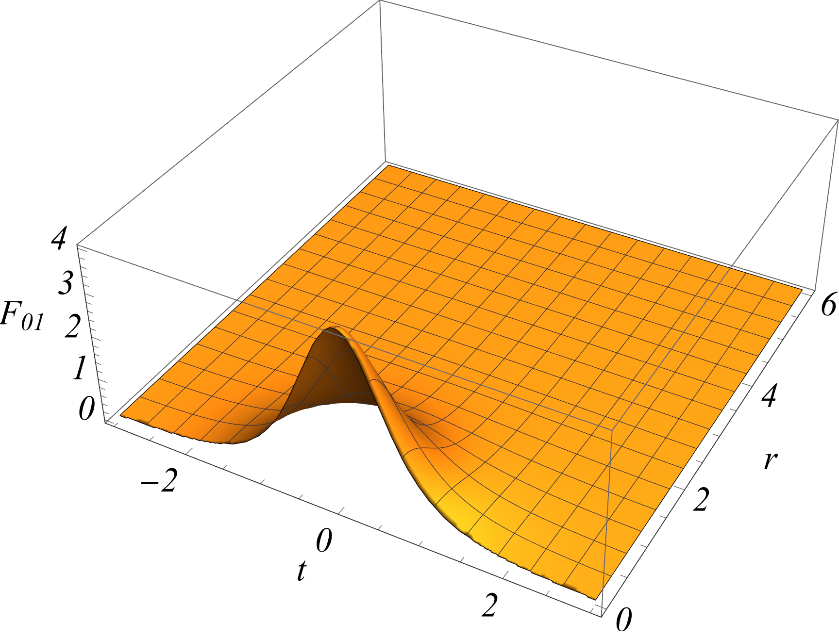
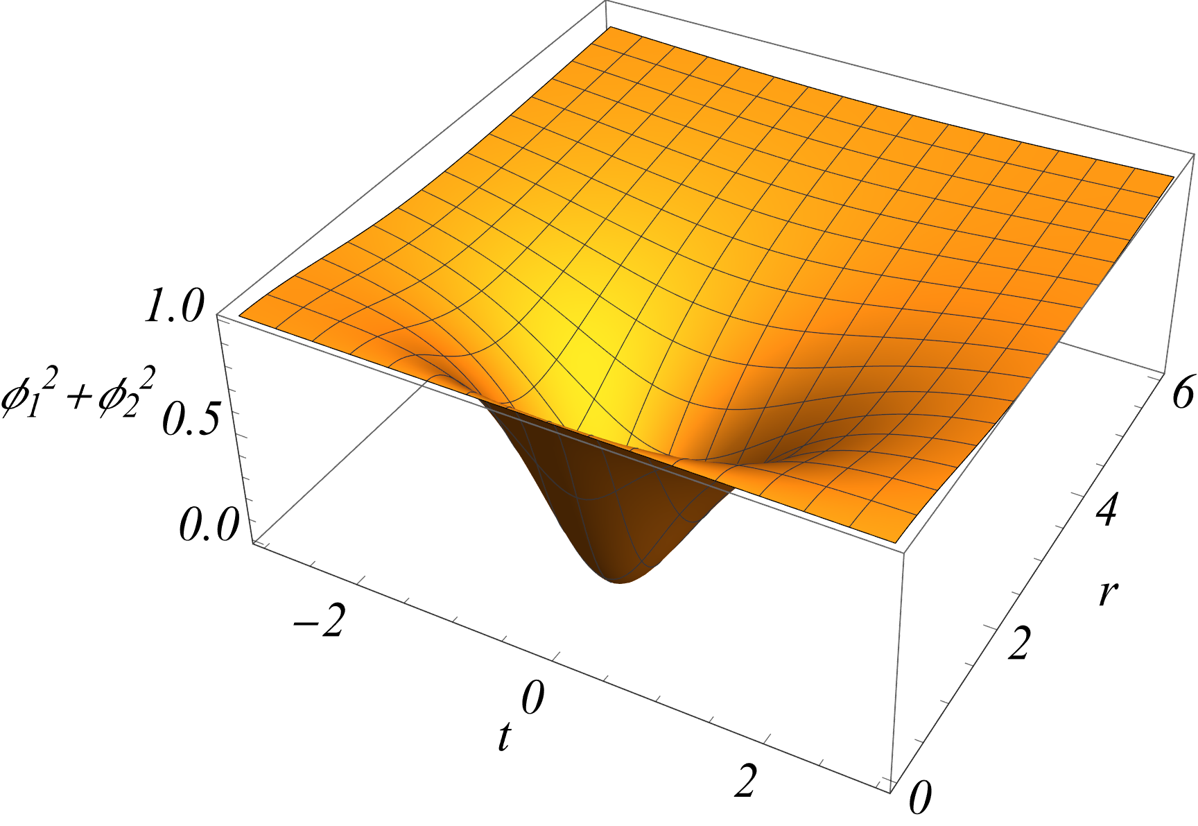
Figure 4: The 1-vortex solution with the center at \((t,r)=(0,1)\) and the size \(\lambda=1\). The distribution of gauge-invariant quantities . (Left) field strength \(F_{tr}(t,r)\), (Right) \(|\phi(t,r)|^2\)..
Proposition [area law of the Wilson loop average[2]] In the dilute gas approximation, the Wilson loop average in the \(\vartheta\) vacuum obeys the area law with the area \(A(C)\) in the semi-classical regime: \[\begin{align} \langle \vartheta | W_C[\mathscr{A}] | \vartheta \rangle = e^{- \sigma A(C)} , \quad \sigma := 2K e^{-S_1/\hbar} \left[ \cos (\vartheta c_2) - \cos \left(\vartheta c_2 + 2\pi J c_1\right) \right] , \label{wler} \end{align}\tag{2}\] where \(c_1\) and \(c_2\) are the first and second Chern numbers corresponding to the vortex number and the Yang-Mills instanton number respectively. Here \(S_1\) is the 1-vortex action, \(J=\frac{1}{2}, 1, \frac{3}{2}, \cdots\) is the index for the representation, and \(K\) is the fugacity of the dilute (instanton) gas. When \(Jc_1\) is an integer, the vacuum is periodic with respect to \(\vartheta c_2\) with period \(2\pi\), so the potential is zero. When \(Jc_1\) is not an integer, the static \(q\bar q\) potential \(V(R)\) has a linear potential \(V(R)=\sigma R\) with the string tension \(\sigma\).
8 Conclusions and discussions↩︎
We considered the space and time symmetric instantons as solutions of the self-dual Yang-Mills equation with conformal symmetry in the \(SU(2)\) Yang-Mills theory in the four-dim. Euclidean space \(\mathbb{R}^4\). In contrast to time translation symmetry, instantons with spatial rotation symmetries give a finite four-dim. action and hence can contribute to quark confinement. For the spatial symmetry \(SO(2) \simeq U(1) \simeq S^1\), the instanton is reduced to a hyperbolic magnetic monopole (of Atiyah) living in the three-dim. hyperbolic space \(\mathbb{H}^3\). For the spatial symmetry \(SO(3) \simeq SU(2)\), the instanton is reduced to a hyperbolic vortex (of Witten-Manton) living in the two-dim. hyperbolic space \(\mathbb{H}^2\).
By requiring the spatial symmetry \(SO(2)\) or \(SO(3)\) for instantons, the four-dim. Euclidean space \(\mathbb{R}^4\) is inevitably mapped to the curved space \(\mathbb{H}^3 \times S^1\) or \(\mathbb{H}^2 \times S^2\) with negative constant curvature by maintaining the conformal equivalence through dimensional reduction. Hyperbolic magnetic monopoles on \(\mathbb{H}^3\) and hyperbolic vortices on \(\mathbb{H}^2\) can be connected through conformal equivalence with the explicit relationship between the magnetic monopole field and the vortex field has been obtained, which allows magnetic monopoles and vortices can be treated in a unified manner.
Both \(\mathbb{H}^3\) and \(\mathbb{H}^2\) are curved spaces \(AdS_3\) and \(AdS_2\) with constant negative curvatures. The hyperbolic monopole in \(\mathbb{H}^3\) is completely determined by its holographic image on the conformal boundary two-sphere \(S_\infty^2\). (This is different from Euclidean monopoles.) This fact enables us to reduce the non-Abelian Wilson loop operator to the Abelian Wilson loop defined by the Abelian gauge field of the vortex: Abelian dominance and magnetic monopole dominance.
Using the hyperbolic magnetic monopole and hyperbolic vortex obtained in this way, quark confinement was shown to be realized in the sense of Wilson area law within the dilute gas approximation. This is a semi-classical quark confinement mechanism originating from the unified hyperbolic magnetic monopole and hyperbolic vortex, supporting the dual superconductor picture.
Acknowledgements↩︎
This work was supported by Grant-in-Aid for Scientific Research, JSPS KAKENHI Grant Number (C) No.23K03406.