Introduction↩︎

The study of singular spaces in differential and algebraic geometry has been approached using various distinct methods. One notable approach involves examining singularities via Lie algebras of vector fields. The investigation of the singularities of singular spaces through their associated Lie algebras of vector fields is a topic with a deep and rich history. This line of inquiry began with the work of Pursell and Shanks [1], who formulated the problem of characterizing a manifold by its Lie algebra of vector fields. Subsequently, similar problems were studied by many authors in different contexts, including H. Omori [2] and J. Grabowski [3]. T. Siebert [4] further developed the work of J. Grabowski [3] (see also [5]–[7] for the superalgebra case), employing a purely algebraic approach in the context of affine varieties. Siebert proved, as a byproduct, the result that an affine variety \(W\) with a ring of coordinates \(\mathcal{O}_W\) is smooth if and only if the Lie algebra \(\mathrm{Der}(\mathcal{O}_W)\) is simple. The direction stating that the smoothness of \(W\) implies the simplicity of \(\mathrm{Der}(\mathcal{O}_W)\) was previously established by D.A. Jordan [8]. These foundational ideas have since inspired further research, emphasizing the utility of Lie-theoretic approaches in understanding both geometric and algebraic structures on a singular space.

The modern approach to geometric problems, as well as to mathematical physics ones, is unified by the language of \(Q\)-structures. The general motto is to replace a singular “hard” object with a collection of “gentle” ones, which are easier to work with. Typically, such a collection comes together with an algebraic structure equipped with a squared-zero operator \(Q\). Hence, the original questions about the singular object might be encoded in the homology of the underlying differential \(Q\). A typical example in differential geometry arises when one considers the intersection of a section of a vector bundle with the base manifold. More precisely, let \(E\to M\) be a vector bundle over a smooth manifold \(M\) and \(s \colon M\to E\), and let \(\Sigma=M\cap \mathrm{Graph}(s)=\{s=0\}\). The latter intersection is singular in general (if \(0\) is not a regular value for \(s\)).

There exists a rather unusual Lie \(\infty\)-algebroid, or equivalently, a negatively graded differential-graded manifold over \(M\), which can be defined by \((\Gamma(\wedge^\bullet E[-1]^*), Q=\iota_s)\) where \(\iota_s\) is the contraction with \(s\). Here, the dual vector bundle \(E[-1]^*\to M\) is concentrated in degree \(-1\). It is clear that the \(0\)-th homology is \(H^0((\Gamma(\wedge^\bullet E[-1]^*), Q))\simeq~C^{\infty}(M)/\mathcal{I}_s\) with \(\mathcal{I}_s\) being the ideal generated by functions of the form \(\langle \xi, s\rangle\) for \(\xi\in \Gamma(E^*)\). If \(s\) is transverse to the zero section, then \(\Sigma\) is smooth and the cohomology of \((\Gamma(\wedge^\bullet E[-1]^*), Q)\) is concentrated in degree \(0\) and \(H^0\) essentially recovers \(C^\infty(\Sigma)\). Therefore, \((\Gamma(\wedge^\bullet E[-1]^*), Q)\) serves a replacement for the singular space \(\Sigma\). In a similar fashion, it is possible to adjust the construction for the common zero locus of several sections \(s_1, \ldots, s_k\in \Gamma(E)\). For example, for \(M=\mathbb{C}^d\) and \(E=\mathbb{C}^d\times \mathbb{C}^n\), the set \(\Sigma\subset \mathbb{C}^d\) is the zero locus of some functions \(\varphi_1,\ldots, \varphi_n\in \mathbb{C}[x_1, \ldots, x_d]\). Here, we have \[Q=\sum_{i=1}^n\varphi_i\frac{\partial}{\partial \eta_i}\;\;\text{and} \;\; H^0((\Gamma(\wedge^\bullet E[-1]^*), Q))\simeq C^{\infty}(M)/\langle \varphi_1,\ldots, \varphi_n \rangle.\] where \(\eta_1,\ldots, \eta_n\) corresponding to the dual basis of \(E[-1]\). One can always choose a negatively graded dg-variety so that there is no homology in degree less than or equal to –1, namely a Koszul-Tate resolution of \({C^\infty(M)}/\mathcal{I}_s\). More generally, to any unital commutative algebra \(\mathcal{O}\) and a proper ideal \(\mathcal{I}\subset \mathcal{O}\) one can associate a Koszul-Tate resolution of \(\mathcal{O}/\mathcal{I}\), which is a graded symmetric dg-algebra \((S_{\mathcal{O}}(\oplus_{i\leq -1} \mathcal{V}_i), \delta)\) acyclic in negative degrees [9]. Such a negative \(Q\)-variety is a cornerstone of BV and BFV formalisms in mathematical physics [10]–[12].

From the infinitesimal point of view, a (regular) foliation \(F \subset TM\) may be encoded as a positively graded \(Q\)-manifold – the leaf-wise de Rham complex \((\Gamma(\wedge^\bullet F^{*}), d^{{DR}})\). The degree-\(0\) cohomology of the latter identifies with the algebra of functions on the (typically singular) leaf space \(M/F\). Similar constructions exist for foliations with singularities, i.e., singular foliations [13], [14] and for vector fields on singular spaces: one replaces \(F\) by an appropriate Lie \(\infty\)-algebroid. Recently, Laurent-Gengoux, Lavau, and Strobl [15] introduced an important framework by associating a class of positively graded \(Q\)-varieties (equivalently negatively graded Lie \(\infty\)-algebroids) to any Lie subalgebra \(\mathfrak A\) of the sheaf of vector fields \(\mathfrak X\) on a manifold \(M\) that admits a geometric resolution, i.e., those for which there exists an anchored complex of vector bundles

\[(E,\mathrm{d}, \rho) \colon \xymatrix{ \ar[r] & E_{-i-1} \ar[r]^{{\mathrm{d}^{(i+1)}}} \ar[d] & E_{ -i} \ar[r]^{{\mathrm{d}^{(i)}}} \ar[d] & E_{-i+1} \ar[r] \ar[d] & \ar@{..}[r] & \ar[r]^{{\mathrm{d}^{(2)}}}& E_{-1} \ar[r]^{\rho} \ar[d]& TM \ar[d] \\ \ar@{=}[r] & \ar@{=}[r] M & \ar@{=}[r] M & \ar@{=}[r] M &\ar@{..}[r] & \ar@{=}[r] & \ar@{=}[r] M & M}\] such that the following complex of sheaves \[\label{}{\longrightarrow} \Gamma({E_{ -i-1}}) \stackrel{\mathrm{d}^{(i+1)}}{\longrightarrow} \Gamma({E_{-i}}) \stackrel{\mathrm{d}^{(i)}}{\longrightarrow}{\Gamma(E_{-i+1})}{\longrightarrow}\cdots {\longrightarrow} \Gamma(E_{-1}) \stackrel{\rho}{\longrightarrow} \mathfrak A\longrightarrow 0\tag{1}\] is exact. It is quite natural to work with this class of Lie sublagebras, as it contains the class of Lie subalgebras that are (locally) real analytic [15]. It is also a natural object in the holomorphic setting, since \(\mathfrak A\) is then a coherent sheaf and such geometric resolutions always exist locally. This construction admits a generalization [16], [17] in a purely algebraic setting, where \(\mathfrak A\) is an arbitrary Lie-Reinhart algebra. With this generalization, we associate a class of positively graded \(Q\)-varieties to any singular space where the concept of vector fields is well-defined, e.g., an affine variety.

It is natural to ask

A positive answer to this question was given in [18] in the smooth geometric setting, i.e., for an ideal \(\mathcal{I}\) of a ring of smooth functions \(\mathcal{O}= C^{\infty}(M)\). However, the result [18] is only an existence result. It is typically expected that a generic Koszul-Tate resolution \((S_{\mathcal{O}}(\oplus_{i\leq -1}\mathcal{V}_i), \delta)\) has infinitely many non-zero \(\mathcal{V}_i\). Thus, finding examples is problematic. Therefore, it is of interest to study the following question:

Questions similar to Question 2 were extensively studied in the realm of projective resolutions of modules. More precisely, in the works of [19], [20] and references therein, an efficient machinery was developed to study monomial resolutions of polynomial rings. A manifest description reveals underlying structures, such as a semi-simplicial complex that governs such resolutions. Moreover, the construction of such resolutions and related computations can now be performed by software [21]. In what concerns Koszul-Tate resolutions, a recent work [22], [23] suggested a construction built on top of projective resolutions of \(\mathcal{O}/\mathcal{I}\). This construction, called an arborescent Koszul-Tate resolution, significantly reduces the number of computations, which becomes finite if the projective resolution is of finite length and has finite ranks at each degree. A manifest description provides insight into the generic structure of any Koszul-Tate resolution [23]. Namely, any Koszul-Tate resolution \((S_{\mathcal{O}}(\oplus_{i\leq -1}\mathcal{V}_i), \delta)\) of \(\mathcal{O}/\mathcal{I}\), where \(\mathcal{O}\) is a polynomial ring and \(\mathcal{I}\) is a monomial ideal, has \(\mathcal{V}_i \neq 0\) for all \(i\) provided that \(\mathcal{I}\) is not generated by a regular sequence.

We address Question 2 in the following setting: as a negative dg-variety we use an arborescent Koszul-Tate resolution of \(\mathcal{O}/\mathcal{I}\), while the positive graded \(Q\)-variety is either a generic one over \(\mathcal{O}/\mathcal{I}\), or it is over \(\mathcal{O}\) and preserves \(\mathcal{I}\). In §1 we recall the notions of \(Q\)-varieties, and recall (arborescent) Koszul-Tate resolutions. In §2 we state the main results of the paper. In §3, we give manifest examples of our construction. In §4 we substitute the arborescent Koszul-Tate resolution by the Koszul complex and draw a comparison from our construction to it. In §5 we give examples of new structures (higher-order multiplications) that our construction induces. In §6 we address the issue of lifting derivations from quotient algebras.
Acknowledgements. We thank C. Laurent-Gengoux, A. Kotov, L. Ryvkin and V. Salnikov for helpful discussions and valuable comments on the manuscript. We are also grateful to E. Lerman for insightful discussions. Finally, R. Louis acknowledges full financial support through the J. L. Doob Research Assistant Professor position at the University of Illinois Urbana–Champaign (UIUC).
Statements and Declarations. The authors have no conflict of interest that is relevant to the content of this article.
Data Availability. Data sharing is not applicable to this article as no datasets were generated or analyzed during the current study.

1 Definitions↩︎

Throughout this article, \(\mathcal{O}\) is a commutative unital algebra over a field \(\mathbb{K}\) of characteristic zero, and \({\mathrm{Der}}(\mathcal{O})\) stands for its Lie algebra of \(\mathbb{K}\)-linear derivations. We denote by \(X[f]\) the derivation \(X \in {\mathrm{Der}}(\mathcal{O})\) applied to \(f\in \mathcal{O}\). Also, an \(\mathcal{O}\)-module \(\mathcal{V}\) is seen as a \(\mathbb{K}\)-vector space in the natural way, for \(\lambda\in \mathbb{K}\), \(\lambda \cdot v := (\lambda \cdot 1_{\mathcal{O}})\, v\), where \(1_{\mathcal{O}} = 1\) is the multiplicative identity of \(\mathcal{O}\). In the sequel, we will drop the notation “\(\cdot\)”.

Geometrically, \(\mathcal{O}\) can be understood as the algebra of smooth functions on a manifold \(M\), or on an open subset \(U \subset M\) of a complex manifold, or the coordinate ring of an affine variety \(W\).
Some notations. Recall that a \(\mathbb{Z}\)-graded \(\mathcal{O}\)-module is an \(\mathcal{O}\)-module of the form \(\mathcal{V}=\oplus_{i \in \mathbb{Z}}\mathcal{V}_i\) for \(\mathcal{O}\)-modules \(\mathcal{V}_i, i\in \mathbb{Z}\). Elements of \(\mathcal{V}_i\) are called homogeneous of degree \(i\). A graded algebra \(\mathcal{A}=\oplus_{i\in \mathbb{Z}}\mathcal{A}_i\) over \(\mathcal{O}\) is a graded \(\mathcal{O}\)-module equipped with a multiplication that respects the grading, i.e., \(\mathcal{A}_i \cdot \mathcal{A}_j \subset \mathcal{A}_{i+j}\). In this paper, we deal with the graded symmetric algebra of a graded module. To fix the sign conventions and notations, let us recall the construction.

For a graded \(\mathcal{O}\)-module \(\mathcal{V}\), we denote by \(\lvert x\rvert \in \mathbb{Z}\) the degree of a homogeneous element \(x\in \mathcal{V}\).

• We denote by \(S_{}(\mathcal{V})\) and call graded symmetric algebra of \(\mathcal{V}\) over \(\mathcal{O}\) the quotient of the tensor algebra over \(\mathcal{O}\) \[T_{}(\mathcal{V}):= \oplus_{k =1}^\infty \underbrace{ \mathcal{V}\otimes_\mathcal{O} \cdots \otimes_\mathcal{O} \mathcal{V}}_{\small{k times}}\] by the ideal generated by \(x\otimes_{\mathcal{O}} y-(-1)^{\lvert x\rvert\lvert y\rvert}y\otimes_{\mathcal{O}} x\), with \(x,y\) arbitrary homogeneous elements of \(\mathcal{V}\). We denote by \(\odot_{\mathcal{O}}\) the product in \(S_{}(\mathcal{V})\). In order to simplify notations we omit the subscript \(\mathcal{O}\) of tensor products \(\otimes_{\mathcal{O}}, \odot_{\mathcal{O}}\), so that these products \(\otimes, \odot\) are understood to be over \(\mathcal{O}\).

• We denote by \(S_R( \mathcal{V})\) the graded symmetric algebra of \(\mathcal{V}\) tensored with the quotient algebra \(R = \mathcal{O}/\mathcal{I}\) for some proper ideal \(\mathcal{I}\subset \mathcal{O}\), namely, \(S_R( \mathcal{V}) = S( \mathcal{V})\otimes_\mathcal{O}R\).

The algebra \(S(\mathcal{V})\) comes equipped with different notions of degrees that must not be confused.

1. We define the degree of \(x= x_1 \odot \cdots \odot x_n\in S^n(\mathcal{V})\mathrel{\vcenter{:}}= \underbrace{ \mathcal{V}\odot \cdots \odot \mathcal{V}}_{\small{n times}}\) by \[| x_1 \odot \cdots \odot x_n | = |x_1|+ \cdots + |x_n|\] for any homogeneous elements \(x_1, \dots, x_n\in\mathcal{V}\). With respect to this degree, \(S(\mathcal{V})\) is a \(\mathbb{Z}\)-graded commutative algebra over \(\mathcal{O}\). For any homogeneous elements \(x_1 , \ldots , x_k \in \mathcal{V}\) and \(\sigma\in\mathfrak{S}_k\) a permutation of \(\{1, \ldots, k\}\), the Koszul sign \(\epsilon(\sigma; x_1 , \ldots , x_k )\) is defined by: \[x_{\sigma(1)} \odot \cdots \odot x_{\sigma(k)}= \epsilon(\sigma; x_1 , \ldots , x_k ) \, x_1 \odot \cdots \odot x_k.\] We write \(\epsilon(\sigma )\) for \(\epsilon(\sigma; x_1 , \ldots , x_k )\).

2. The polynomial degree of \(x_1 \odot \cdots \odot x_n\in S^n(\mathcal{V})\) is defined to be \(n\). Elements of polynomial degree \(k\) and degree \(d\) in \(S(\mathcal{V})\) are denoted by \(S^k(\mathcal{V})_d\).

3. There is also a notion of “positive” and “negative” gradings in \(S(\mathcal{V})\). For an element \(a \in \mathcal{V}_i\) we prescribe them as follows: \[|a|_- = \begin{cases} 0, \quad if \; i\geq 0, \\ -i, \quad if \; i<0. \end{cases}\] \[|a|_+ = \begin{cases} i, \quad ifi \geq0, \\ 0, \quad ifi < 0. \end{cases}\] So that \(|a| = |a|_+ - |a|_-\). The degrees \(|\,\cdot \,|_+\,\,,\,\, |\,\cdot \,|_-\) are extended to elements of \(S(\mathcal{V})\) by the formula \(|ab|_k = |a|_k + |b|_k\), where \(a,b\) are monomials of \(S(\mathcal{V})\), with \(k \in \lbrace +, - \rbrace\). A homogenous element of negative degree \(i\) is denoted as \(w_{(i)}\). For instance, elements of \(\mathcal{V}_{1}\odot \mathcal{V}_{-4}\) are of

   1. degree \(-3\);

   2. polynomial degree \(2\);

   3. negative degree \(4\);

   4. positive degree \(1\).

• Every linear map \(\Phi\colon S(\mathcal{V}) \to S(\mathcal{V}')\) between graded symmetric algebras admits a decomposition w.r.t the degree, as well as the negative degree. We denote by \(\Phi_k\) (respectively \(\Phi_{(k)}\)) the component of \(\Phi\) of degree \(k\) (negative degree \(k\)), which means that it sends an element \(a_i\) to an element of degree \(i+k\) (or \(a_{(i)}\) to \((\Phi(a_{(i)}))_{(i+k)}\)).

• A derivation of degree \(k\) is a \(\mathbb{K}\)-linear map \(Q\colon S(\mathcal{V}) \to S(\mathcal{V})\) satisfying the graded Leibniz rule, i.e., \[Q(a\odot b) = Q(a)\odot b + (-1)^{k|a|}a\odot Q(b)\] for homogeneous elements \(a\) and \(b\) of \(S(\mathcal{V})\). Such a derivation admits a decomposition with respect to the negative degree \[Q = \sum_{i\in \mathbb{Z}}Q_{(i)}\] where \(Q_{(i)}\colon S(\mathcal{V})\to S(\mathcal{V})\) is a derivation of \(S(\mathcal{V})\) of negative degree \(i\) and of degree \(k\).

1.1 \(\mathbb{Z}\)-graded \(Q\)-varieties↩︎

When working with \(\mathbb{Z}\)-graded algebras, one is quickly led to consider infinite sums of homogeneous elements. It therefore becomes essential to specify which such infinite sums are meaningful, that is, to determine a notion of convergence. For instance, in the smooth geometrical setting, for \(\mathbb{Z}\)-graded manifolds, one would like to perform change of coordinates, e.g., \(x_i \mapsto x_i + \eta \mathcal{P}\), where \(x=(x_1, \ldots, x_n)\) is a local coordinate on a manifold \(M\), and \(\eta, \mathcal{P}\) are graded coordinates of degrees \(2\) and \(-2\) respectively. Then the Taylor series for \(\sin (x_1 + \eta \mathcal{P})\) does not make sense³ in \(S(\mathcal{V})\). In our paper, this issue arises when doing homological perturbation – we obtain homogeneous components of an \(\mathcal{O}\)-linear map \(\Phi\). In particular, if there are infinitely many components \(\Phi_{(k)}\) of negative degree \(k\) and of fixed degree \(i\), then the sum \(\sum_{k\in \mathbb{Z}} \Phi_{(k)}(a)\), \(a\in \mathcal{V}\), does not make sense in \(S(\mathcal{V})\). Therefore it is necessary to find an appropriate completion of \(S(\mathcal{V})\) for which our construction converges. This necessity naturally leads to the introduction of filtrations and their associated topologies. For the sake of clarity in our notation and conventions, we recall the following

If our graded commutative unital algebra is concentrated in negative degrees, we do not want the completion to alter the algebra, as happens in the Laurent-type example in Remark 4 (2). To remedy this, we shall consider completion by degree, i.e., we complete at each degree separately with respect to the negative filtration. More precisely, let \(\mathcal{G} = \oplus_{j\in \mathbb{Z}} \mathcal{G}_j\) be a \(\mathbb{Z}\)-graded commutative unital algebra and \(\hat{\mathcal{G}}\) its completion w.r.t the negative filtered topology. We shall denote by \(\Bar{\mathcal{G}}=\oplus_{j\in \mathbb{Z}} \Bar{\mathcal{G}}_j\) the \(\mathbb{Z}\)-graded commutative unital subalgebra of \(\hat{\mathcal{G}}\) obtained by a “degree by degree” completion of \(\mathcal{G}\) w.r.t the negative filtered topology, that is, for every \(j\in \mathbb{Z}\)

\[\bar{\mathcal{G}}_j=\{\text{the equivalence classes of all the Cauchy sequences of \mathcal{G}_j}\}.\]

Now, \[\label{eq:proj95lim95R} \bar{\mathcal{G}}= \oplus_{i\in \mathbb{Z}} \varprojlim_{j}\Big(\mathcal{G}_i/F^j \mathcal{G}_i\Big)\tag{3}\] here, \(F^j \mathcal{G}_i\) stands for the vector space of elements of degree \(i\) in \(F^j \mathcal{G}\).

The following proposition is important and will be used to ensure convergence in our main results.

We consider the following definition of a \(\mathbb{Z}\)-graded manifold/variety. Their properties are carefully studied in [26].

In Definition 1, the vector bundles \((V_i)_{i\in \mathbb{Z}^\times}\) are only defined on an open neighborhood of a point. However, Batchelor’s theorem for \(\mathbb{Z}\)-graded manifold [18], [26]–[28] says in the smooth case that they can be glued into global vector bundles \((E^*_i)_{i\in \mathbb{Z}^\times}\) on \(M\) such that \(\mathcal{A}\simeq \Gamma( S(\oplus_{i\in \mathbb{Z}^\times} E^*_{i}))\). The vector bundles \((E_{i})_{i\in \mathbb{Z}^\times}\) are canonically defined by Serre-Swan theorem so that the modules of sections of their duals \((E_i^*)_{i\in \mathbb{Z}^\times}\) are \(\mathcal{I}/\mathcal{I}^2=\left(\mathcal{I}_{-i}/(\mathcal{I}^2)_{-i}\right)_{i\in \mathbb{Z}^\times}\), where \(\mathcal{I}=\mathcal{I}_{-}+\mathcal{I}_{+}\) with \(\mathcal{I}_{-}\) resp. \(\mathcal{I}_{+}\) is the ideal of \(\mathcal{A}\) generated by negative/positive homogeneous degree functions [18], [26]. In the sequel, our graded manifold will be of this form, under a choice of such an isomorphism. This choice will be referred to as a splitting.

This justifies an algebraic version of the Definition 1.

Given a \(\mathbb{Z}\)-graded variety \(\mathcal{A} \mathrel{\vcenter{:}}= \bar{S}\!\left(\oplus_{i \in \mathbb{Z}^\times} \mathcal{V}_i\right),\) the derivations of \(\mathcal{A}\), equipped with the graded commutator, form a graded Lie algebra \(\mathrm{Der}(\mathcal{A})\).

Given a split \(\mathbb{Z}\)-graded manifold \(\mathcal{A}\simeq \Gamma (\bar S(\oplus_{i\in \mathbb{Z}^\times} E^*_i))\) we shall denote by \(\mathfrak X({E})\) the \(\mathbb{Z}\)-graded derivations of \(\mathcal{A}\), they shall be called (graded) vector fields on \(E\).

1.1.1 The negative and positive components of a \(\mathbb{Z}\)-graded \(Q\)-variety↩︎

Let \((\mathcal{A}, Q)\) be a \(\mathbb{Z}\)-graded \(Q\)-variety. The pair \((\mathcal{A}, Q)\) breaks into two main components: a negative component, which is a negatively graded \(Q\)-variety that is denoted by \((\mathcal{A}^-,Q^-)\), and a positive component, which is a \(\mathbb{N}\)-graded \(Q\)-variety as well, that we denote by \((\mathcal{A}^+,Q^+)\). Let us now recall how these components are defined.

1. The negative component \((\mathcal{A}^-,Q^-)\) of \((\mathcal{A}, Q)\). This component is essentially constructed by modding out the ideal of positively graded functions. More precisely, consider an ideal \(\mathcal{I}_+\) of \(\mathcal{A}\) generated by positive homogeneous degree functions \(\mathcal{A}_{\geq +1}\). We define \(\mathcal{A}^-\) to be the quotient \(\mathcal{A}/\mathcal{I}_+\). Since the degree of the homological vector field \(Q\) is \(+1\), it preserves the ideal \(\mathcal{I}_+\) , i.e., \(Q[\mathcal{I}_+]\subset \mathcal{I}_+\). Hence, \(Q\) passes to quotient and yields a well-defined homological vector field \(Q^-\) of degree \(+1\). Therefore, the pair \((\mathcal{A}^-, Q^-)\) is a negatively graded \(Q\)-variety that we call the negative component of \((\mathcal{A}, Q)\). Notice that the vector field \(Q^-\) is vertical, i.e., it is \(\mathcal{O}\)-linear.

2. The positive component \((\mathcal{A}^+,Q^+)\) of \((\mathcal{A}, Q)\). Consider the ideal \(\mathcal{I}_-\) of \(\mathcal{A}\) generated by negative homogeneous degree functions \(\mathcal{A}_{\leq -1}\). Unlike the negative component of \((\mathcal{A}, Q)\), the vector field \(Q\) does not immediately descend to the positively graded manifold \(\mathcal{A}/\mathcal{I}_-\), since \(Q(\mathcal{A}_{-1})\subset \mathcal{A}_0\). However, the ideal \(\mathcal{I}_-+Q[\mathcal{I}_{-}]\) is preserved by \(Q\). \(\mathcal{A}^+\) is defined as the quotient \(\mathcal{A}/(\mathcal{I}_-+Q[\mathcal{I}_{-}])\). The explicit description of \(\mathcal{A}^+\) is as follows: let \(\mathcal{I}\) be an ideal of \(\mathcal{O}\) given by the image

   where \(\mathrm{pr}_{(0)}\) is the projection on negative degree \(0\). Then a straightforward observation shows that \(\mathcal{I}_-+Q[\mathcal{I}_{-1}]=\mathcal{I}_-+\mathcal{I}\mathcal{A}\), [18]. Therefore, if \(\mathcal{A}= \bar S({\oplus_{i\in \mathbb{Z}^\times}\mathcal{V}_i})\), then the positive component \((\mathcal{A}^+, Q^+)\) of \((\mathcal{A}, Q)\) is identified as \(\mathcal{A}^+ = S_{\mathcal{O}/\mathcal{I}}(\oplus_{i\geq 0}\mathcal{V}_i)\) and \(Q^+\) is \(Q\) descended to the quotient.

1.2 Lie-Rinehart algebras and positively graded \(Q\)-varieties↩︎

Let \(\mathcal{O}\) be a commutative unital algebra over \(\mathbb{K}=\mathbb{R}\) or \(\mathbb{C}\). Which geometrically may correspond to an algebra of admissible functions of a manifold or an affine variety.

Restriction. Consider a Lie-Rinehart algebra \((\mathfrak A, [\cdot, \cdot]_\mathfrak A , \rho_{\mathfrak A})\) over \(\mathcal{O}\). For every Lie-Rinehart ideal \(\mathcal{I} \subset \mathcal{O}\), i.e. any ideal such that \[\rho_\mathfrak A (\mathfrak A) [\mathcal{I}] \subset \mathcal{I}\] the quotient space \(\mathfrak A / \mathcal{I} \mathfrak A\) inherits a natural Lie-Rinehart algebra structure over \(\mathcal{O} / \mathcal{I}\). We call this Lie-Rinehart algebra the restriction w.r.t the Lie-Rinehart ideal \(\mathcal{I}\). In the context of affine varieties or an arbitrary subset \(\Sigma\subseteq M\) of a manifold, when \(\mathcal{I}\) is the ideal of functions vanishing on \(\Sigma\), we shall denote \(\frac{\mathfrak A}{\mathcal{I}\mathfrak A}\) by \(\mathfrak i_{\Sigma}^* \mathfrak A\).

It is natural to ask whether, given a Lie–Rinehart algebra \(\mathfrak{A}\) over \(\mathcal{O}/\mathcal{I}\), there exists a \(\mathbb{Z}\)-graded \(Q\)-variety \((\mathcal{A}, Q)\) over \(\mathcal{O}\) whose basic Lie–Rinehart algebra is precisely \(\mathfrak{A}\). The answer to this question is provided in Theorem 5. In that theorem, \((\mathcal{A}, Q)\) is constructed so that its negative part is an arborescent Koszul–Tate resolution of \(\mathcal{O}/\mathcal{I}\), while its positive part is a universal positively graded \(Q\)-variety associated to \(\mathfrak{A}\), which we recall below.

As a consequence, we obtain the following.

1.3 Arborescent Koszul-Tate resolutions↩︎

An important class of examples of negatively graded \(Q\)-varieties/manifolds is the so-called Koszul-Tate resolution of \(\mathcal{O}/\mathcal{I}\) for some proper ideal \(\mathcal{I}\) of an algebra \(\mathcal{O}\). Koszul-Tate resolutions are also known in a more algebraic setting, see [9] for a historical introduction.

A standard way to construct a Koszul-Tate resolution \((S(\mathcal{V}), \delta)\) of \(\mathcal{O}/\mathcal{I}\) is to employ the Tate algorithm [9]. The main idea is to consistently extend a differential graded commutative algebra (dgca) \(S(\mathcal{V}_{-1}\oplus \dots \oplus \mathcal{V}_{-k})\) equipped with a differential of degree \(+1\) \[\delta^{-k}\colon S(\mathcal{V}_{-1}\oplus \dots \oplus \mathcal{V}_{-k})\to S(\mathcal{V}_{-1}\oplus \dots \oplus \mathcal{V}_{-k})\] to a dgca \(\left(S(\mathcal{V}_{-1}\oplus \dots \oplus \mathcal{V}_{-k} \oplus \mathcal{V}_{-k-1}), \delta^{-k-1}\right)\) such that

• \(\delta^{-k-1}\) coincides with \(\delta^{-k}\) on \(\mathcal{V}_{-1}\oplus \dots \oplus \mathcal{V}_{-k}\).

• \(H^{-k}(S(\mathcal{V}_{-1}\oplus \dots \oplus \mathcal{V}_{-k}\oplus \mathcal{V}_{-k-1}),\; \delta^{-k-1}) = 0\). In other words, all non-trivial cycles of degree \(-k\) of \((S(\mathcal{V}_{-1}\oplus \dots \oplus \mathcal{V}_{-k},\; \delta^{-k})\) are in the image \(\delta^{-k-1}(\mathcal{V}_{-k-1})\).

Despite its apparent simplicity, this algorithm, in general, does not terminate even for Noetherian \(\mathcal{O}\). For such \(\mathcal{O}\) all \(\mathcal{V}_{-j}\) can be chosen to be finitely generated, but one still deals with an infinite collection of them, at least for \(\mathcal{O}\) being a polynomial ring and a monomial ideal \(\mathcal{I}\subsetneq \mathcal{O}\) [23]. An alternative approach is given by arborescent Koszul-Tate resolutions [23] which are obtained from a projective resolution \((\mathfrak M, d)\) of \(\mathcal{O}/\mathcal{I}\), which is simpler in a number of examples. By projective resolution \((\mathfrak M, d)\) we mean a sequence of projective \(\mathcal{O}\)-modules \((\mathfrak M_i)_{i<0}\) such that \[\begin{tikzcd} \cdots \arrow[r,"d"] & \mathfrak M_{-i}\arrow[r,"d"] & \cdots \arrow[r, "d"] & \mathfrak M_{-1} \arrow[r, "d"] & \mathcal{O}\arrow[r] & 0 \end{tikzcd}\] is acyclic in negative degrees and \(H^{0}(\mathfrak M, d) = \mathcal{O}/\mathcal{I}\). We shall fix a projective resolution \((\mathfrak M, d)\) of \(\mathcal{O}/\mathcal{I}\) in the sequel. Let us briefly recall the construction.

1.3.1 The construction↩︎

In this section we use the notations and conventions of [23].

1. The starting point is the set of planar rooted trees, i.e., trees that can be embedded in a plane with a distinguished vertex, labeled as the root, at the bottom of the tree. There is a natural partial ordering on the vertices (nodes) of such trees: \(A<B\) if the unique path from the root to the node \(B\) passes through \(A\). Such \(A\) is called an ascendant of \(B\) (and \(B\) is a descendant of \(A\)). If \(A<B\) and there are no vertices on the path from \(A\) to \(B\), i.e., \(A\) and \(B\) are connected by an edge, then \(A\) is called the parent of \(B\), while \(B\) is called a child of \(A\). The maximal elements w.r.t the partial ordering "\(<\)" are referred to as leaves, the minimal one is the root, while to others we refer to as inner vertices.

   The terminology above is illustrated in the Figure [fig:trees1]. \(A\) is an ascendant of \(B\), \(B\) is a leaf vertex. \(E\) is the root vertex of the second tree, and it is a parent of vertices \(C\) and \(D\). \(G\) is a leaf and a child of \(D\). We label the root vertex as well as inner vertices by \(\bullet\). Leaves are not marked by \(\bullet\).

2. The next step is to consider a \(\mathbb{K}\)-vector space \(Tree\) of planar rooted trees, satisfying an additional condition that the valency (i.e., the number of edges connected to the vertex) of each inner vertex \(\geq 3\) and the root valency is \(\geq 2\). This space is enlarged by a trivial tree, which, by our conventions, consists of only one leaf.

Examples of such trees are depicted below:

It is our convention to visualize the trivial tree as “leaf” + “edge”. The first tree in Figure [fig:trees1] is not admissible, since the root valency is \(1\).

Module of planar rooted decorated trees: Denote \(Tree^n\) the \(\mathbb{K}\)-subspace of \(Tree\) of trees with \(n\) leaves. Let us describe the \(\mathcal{O}\)-module of planar rooted trees decorated with \((\mathfrak M, d)\). We set \[Tree[\mathfrak M]\mathrel{\vcenter{:}}= \oplus_{n=1}^{\infty} Tree^n \otimes_{\mathbb{K}} \mathfrak M^{\otimes n}.\] Here, \(\mathfrak M^{\otimes n}\) stands for the tensor product over \(\mathcal{O}\) of \(\mathfrak M\) taken with itself \(n\)-times. The \(\mathcal{O}\)-module structure of \(Tree[\mathfrak M]\) is obvious. Since the number of leaves is equal to the tensor power of \(\mathfrak M\), it is useful to interpret elements of the \(\mathcal{O}\)-module \(Tree[\mathfrak M]\) as planar trees with leaves decorated (labeled) by elements of \(\mathfrak M\). We denote by \(t[a_1, \dots, a_n]\) the element \(t\otimes_{\mathbb{K}} a_1 \otimes \dots \otimes a_n \in Tree[\mathfrak M]\), where \(t\) is a rooted tree \(\in Tree^n\) decorated with \(a_1 \otimes \dots \otimes a_n\). The homological degree of a tree \(t\in Tree^n\) decorated by elements \(a_1, \dots, a_n\) of homogeneous degree is given by \[|t[a_1, \dots, a_n]| =- root \# -\# (of inner vertices of t)+ |a_1| + \dots +|a_n|.\] Here the root \(\#\) is equal to \(0\) or \(1\), depending on whether the tree is trivial (root \(\# = 0\)) or not (root \(\# = 1\)). In particular, for trees \[t_1[a_1, \dots, a_5] = \adjustbox{valign =c }{ \scalebox{0.5}{ \begin{forest} for tree = {grow' = 90}, nice empty nodes, for tree={ inner sep=5 pt, s sep= 5 pt, fit=band, }, [ [\scalebox{2}{a_1}, tier =1] [\scalebox{2}{a_2}, tier =1] [ [\scalebox{2}{a_3}, tier =1] [\scalebox{2}{a_4}, tier = 1] [\scalebox{2}{a_5}, tier = 1] ] ] \path[fill=black] (.parent anchor) circle[radius=4pt] (!3.child anchor) circle[radius=4pt]; \end{forest} }}, \quadand\quad t_2[a_1] = \adjustbox{valign =c }{ \begin{forest} for tree = {grow' = 90}, nice empty nodes, for tree={ inner sep=5 pt, s sep= 5 pt, fit=band, }, [ [a_1, tier =1] ]; \end{forest}}\] \(|t_1[a_1,\dots, a_5]| = -2 + |a_1| + \dots + |a_5|\) and \(|t_2[a_1]| = |a_1|\). For \(n\in \mathbb{N}\), we denote by \(Tree[\mathfrak M]_{-n}\) the subspace of decorated trees of degree \(-n\). Clearly, \(Tree[\mathfrak M] = \oplus_{n\in \mathbb{N}}Tree[\mathfrak M]_{-n}\).

Some operations on rooted decorated trees: The following two natural operations on rooted trees are employed in the construction of the arborescent Koszul-Tate resolution. The first one is the isomorphism \[T^{\geq 2}(Tree[\mathfrak M]) \cong Tree^{\geq 2}[\mathfrak M]\] provided by the root map \(\mathfrak r\colon T^{\geq 2}(Tree[\mathfrak M]) \cong Tree^{\geq 2}[\mathfrak M]\). Graphically, \(\mathfrak r\) tantamounts to joining the forest of trees into a tree by means of a root vertex, e.g., \[\mathfrak r\colon \adjustbox{valign =c }{ \scalebox{1}{ \begin{forest} for tree = {grow' = 90}, nice empty nodes, for tree={ inner sep=5 pt, s sep= 5 pt, fit=band, }, [ [\scalebox{1}{a_1}, tier =1] [\scalebox{1}{a_2}, tier =1] ] \path[fill=black] (.parent anchor) circle[radius=2pt]; \end{forest} }} \otimes \adjustbox{valign =c }{ \scalebox{1}{ \begin{forest} for tree = {grow' = 90}, nice empty nodes, for tree={ inner sep=5 pt, s sep= 5 pt, fit=band, }, [ [\scalebox{1}{a_3}, tier =1] [\scalebox{1}{a_4}, tier = 1] [\scalebox{1}{a_5}, tier = 1] ] \path[fill=black] (.parent anchor) circle[radius=2pt]; \end{forest} }} \mapsto \adjustbox{valign =c }{ \scalebox{0.5}{ \begin{forest} for tree = {grow' = 90}, nice empty nodes, for tree={ inner sep=5 pt, s sep= 5 pt, fit=band, }, [ [ [\scalebox{2}{a_1}, tier =1] [\scalebox{2}{a_2}, tier =1] ] [ [\scalebox{2}{a_3}, tier =1] [\scalebox{2}{a_4}, tier = 1] [\scalebox{2}{a_5}, tier = 1] ] ] \path[fill=black] (.parent anchor) circle[radius=4pt] (!1.child anchor) circle[radius=4pt] (!2.child anchor) circle[radius=4pt]; \end{forest} }}\] The other operation, \(\partial_A\colon T^{\geq 2}(Tree[\mathfrak M]) \cong Tree^{\geq 2}[\mathfrak M]\), consists in removing an inner vertex \(A\) of a given decorated tree. This is done by means of merging \(A\) with its parent vertex \(P_A\). For instance, \[\partial_A\colon \adjustbox{valign =c }{ \scalebox{0.5}{ \begin{forest} for tree = {grow' = 90}, nice empty nodes, for tree={ inner sep=5 pt, s sep= 5 pt, fit=band, }, [,{label=[mystyle]{\scalebox{2}{P_A\quad }}} [,{label=[mystyle]{\scalebox{2}{A\quad }}} [\scalebox{2}{a_1}, tier =2] [\scalebox{2}{a_2}, tier =2] ] [ [\scalebox{2}{a_3}, tier =1] [\scalebox{2}{a_4}, tier = 1] [\scalebox{2}{a_5}, tier = 1] ] ] \path[fill=black] (.parent anchor) circle[radius=4pt] (!1.child anchor) circle[radius=4pt] (!2.child anchor) circle[radius=4pt]; \end{forest} }} \mapsto \adjustbox{valign =c }{ \scalebox{0.5}{ \begin{forest} for tree = {grow' = 90}, nice empty nodes, for tree={ inner sep=5 pt, s sep= 5 pt, fit=band, }, [,{label=[mystyle]{\scalebox{2}{P_A\quad }}} [\scalebox{2}{a_1}, tier =2] [\scalebox{2}{a_2}, tier =2] [ [\scalebox{2}{a_3}, tier =1] [\scalebox{2}{a_4}, tier = 1] [\scalebox{2}{a_5}, tier = 1] ] ] \path[fill=black] (.parent anchor) circle[radius=4pt] (!3.child anchor) circle[radius=4pt]; \end{forest} }}\]

Module of symmetric decorated trees: Let \(A\) be any vertex of a tree \(t[a_1,\dots, a_n]\) and let \(\theta_1, \dots, \theta_m\) be the decorated subtrees of \(t\) which are children of \(A\). We set the following equivalence relations: \[\label{eq:sym46trees} t[a_1, \dots, a_n] \sim \epsilon(\sigma, \theta) t[a_{\sigma(1)}, \dots, a_{\sigma(n)}],\tag{5}\] where \(\sigma\) is the permutation of the children of \(A\) and \(\epsilon(\sigma, \theta)\) is the Koszul sign of this permutation with respect to the degrees \(|\theta_1|, \dots, |\theta_m|\). More precisely, \(\epsilon(\sigma,\theta)\) is deduced from the following equation: \[\theta_1 \cdots \theta_m = \epsilon(\sigma, \theta)\cdot\theta_{\sigma(1)}\cdots \theta_{\sigma(m)}.\]

Let us illustrate the equivalence on the following example: \[\adjustbox{valign =c }{ \scalebox{0.5}{ \begin{forest} for tree = {grow' = 90}, nice empty nodes, for tree={ inner sep=5 pt, s sep= 5 pt, fit=band, }, [,{label=[mystyle]{\scalebox{2}{P\quad }}} [,{label=[mystyle]{\scalebox{2}{A\quad }}} [\scalebox{2}{a_1}, tier =2] [\scalebox{2}{a_2}, tier =2] ] [,{label=[mystyle]{\scalebox{2}{B\quad }}} [\scalebox{2}{a_3}, tier =1] [\scalebox{2}{a_4}, tier = 1] ] ] \path[fill=black] (.parent anchor) circle[radius=4pt] (!1.child anchor) circle[radius=4pt] (!2.child anchor) circle[radius=4pt]; \end{forest} }} = (-1)^{(|a_1|+|a_2|+1)(|a_3| +|a_4| +1 )} \adjustbox{valign =c }{ \scalebox{0.5}{ \begin{forest} for tree = {grow' = 90}, nice empty nodes, for tree={ inner sep=5 pt, s sep= 5 pt, fit=band, }, [,{label=[mystyle]{\scalebox{2}{P\quad }}} [,{label=[mystyle]{\scalebox{2}{B\quad }}} [\scalebox{2}{a_3}, tier =1] [\scalebox{2}{a_4}, tier = 1] ] [,{label=[mystyle]{\scalebox{2}{A\quad }}} [\scalebox{2}{a_1}, tier =2] [\scalebox{2}{a_2}, tier =2] ] ] \path[fill=black] (.parent anchor) circle[radius=4pt] (!1.child anchor) circle[radius=4pt] (!2.child anchor) circle[radius=4pt]; \end{forest} }} =(-1)^{|a_1||a_2|} \adjustbox{valign =c }{ \scalebox{0.5}{ \begin{forest} for tree = {grow' = 90}, nice empty nodes, for tree={ inner sep=5 pt, s sep= 5 pt, fit=band, }, [,{label=[mystyle]{\scalebox{2}{P\quad }}} [,{label=[mystyle]{\scalebox{2}{A\quad }}} [\scalebox{2}{a_2}, tier =2] [\scalebox{2}{a_1}, tier =2] ] [,{label=[mystyle]{\scalebox{2}{B\quad }}} [\scalebox{2}{a_3}, tier =1] [\scalebox{2}{a_4}, tier = 1] ] ] \path[fill=black] (.parent anchor) circle[radius=4pt] (!1.child anchor) circle[radius=4pt] (!2.child anchor) circle[radius=4pt]; \end{forest} }}.\]

The first equality is due to the permutation of subtrees with roots \(A\) and \(B\) (which are children of \(P\)), while the second one comes from a permutation of leaves \(|\otimes_{\mathbb{K}}a_1\) and \(|\otimes_{\mathbb{K}}a_2\).

Arborescent Koszul-Tate resolutions: In what follows, we abbreviate elements of \(\mathcal{T} ree[\mathfrak M]\) by a representative in \(Tree[\mathfrak M]\), while bearing in mind that the branches of such trees can be permuted with the Koszul sign. Let \(S(\mathcal{T} ree[\mathfrak M])\) be the graded symmetric algebra of symmetric decorated trees \(\mathcal{T}ree[\mathfrak M]\) in Definition 6. Let us list the first graded components \(\mathcal{T} ree[\mathfrak M]_i =: \mathcal{V}_i\), \(-4\leq i\leq -1\): \[\begin{align} \mathcal{V}_{-1} \mathrel{\vcenter{:}}=& \adjustbox{valign =c }{ \scalebox{0.5}{ \begin{forest} for tree = {grow' = 90}, nice empty nodes, for tree={ inner sep=5 pt, s sep= 5 pt, fit=band, }, [, [ ] ]; \end{forest} }} \otimes_{\mathbb{K}} \mathfrak M_{-1} \\ \mathcal{V}_{-2} \mathrel{\vcenter{:}}=& \adjustbox{valign =c }{ \scalebox{0.5}{ \begin{forest} for tree = {grow' = 90}, nice empty nodes, for tree={ inner sep=5 pt, s sep= 5 pt, fit=band, }, [, [ ] ]; \end{forest} }} \otimes_{\mathbb{K}} \mathfrak M_{-2} \\ \mathcal{V}_{-3}\mathrel{\vcenter{:}}=& \adjustbox{valign =c }{ \scalebox{0.5}{ \begin{forest} for tree = {grow' = 90}, nice empty nodes, for tree={ inner sep=5 pt, s sep= 5 pt, fit=band, }, [, [ ] ]; \end{forest} }} \otimes_{\mathbb{K}} \mathfrak M_{-3} \oplus \adjustbox{valign =c }{ \scalebox{0.5}{ \begin{forest} for tree = {grow' = 90}, nice empty nodes, for tree={ inner sep=5 pt, s sep= 5 pt, fit=band, }, [ [, tier =1] [, tier =1] ] \path[fill=black] (.parent anchor) circle[radius=4pt]; \end{forest} }}\otimes_{\mathbb{K}} \mathfrak M_{-1}\odot \mathfrak M_{-1} \\ \mathcal{V}_{-4}\mathrel{\vcenter{:}}=& \adjustbox{valign =c }{ \scalebox{0.5}{ \begin{forest} for tree = {grow' = 90}, nice empty nodes, for tree={ inner sep=5 pt, s sep= 5 pt, fit=band, }, [, [ ] ]; \end{forest} }} \otimes_{\mathbb{K}} \mathfrak M_{-4} \oplus \adjustbox{valign =c }{ \scalebox{0.5}{ \begin{forest} for tree = {grow' = 90}, nice empty nodes, for tree={ inner sep=5 pt, s sep= 5 pt, fit=band, }, [ [, tier =1] [, tier =1] ] \path[fill=black] (.parent anchor) circle[radius=4pt]; \end{forest} }}\otimes_{\mathbb{K}} \mathfrak M_{-1}\odot \mathfrak M_{-2} \oplus \adjustbox{valign =c }{ \scalebox{0.5}{ \begin{forest} for tree = {grow' = 90}, nice empty nodes, for tree={ inner sep=5 pt, s sep= 5 pt, fit=band, }, [ [, tier =1] [, tier =1] [, tier =1] ] \path[fill=black] (.parent anchor) circle[radius=4pt]; \end{forest} }}\otimes_{\mathbb{K}} \mathfrak M_{-1}\odot \mathfrak M_{-1}\odot \mathfrak M_{-1}. \end{align}\]

The root map \(\mathfrak r\) is consistently defined on this quotient, providing an isomorphism \(\mathfrak r\colon S^{\geq 2}(\mathcal{T} ree[\mathfrak M]) \simeq \mathcal{T} ree^{\geq 2}[\mathfrak M]\).

For \(n=3, m =2\) the derivation \(\delta_{\psi}\) is decoded as follows: \[\delta_{\psi} \left( \adjustbox{valign =c }{ \scalebox{0.5}{ \begin{forest} for tree = {grow' = 90}, nice empty nodes, for tree={ inner sep=5 pt, s sep= 5 pt, fit=band, }, [ [\scalebox{2}{a_1}, tier =1] [\scalebox{2}{a_2}, tier =1] ] \path[fill=black] (.parent anchor) circle[radius=4pt]; \end{forest} }} \right) = a_1 \odot a_2 - \psi \left ( \adjustbox{valign =c }{ \scalebox{0.5}{ \begin{forest} for tree = {grow' = 90}, nice empty nodes, for tree={ inner sep=5 pt, s sep= 5 pt, fit=band, }, [ [\scalebox{2}{a_1}, tier =1] [\scalebox{2}{a_2}, tier =1] ] \path[fill=black] (.parent anchor) circle[radius=4pt]; \end{forest} }} \right)\] For \(n=3\) there are no terms from the second summand in 6 . They do appear, for example, when the decoration \(a_1\) has a degree lower than \(-1\). In particular, \[\delta_{\psi} \left( \adjustbox{valign =c }{ \scalebox{0.5}{ \begin{forest} for tree = {grow' = 90}, nice empty nodes, for tree={ inner sep=5 pt, s sep= 5 pt, fit=band, }, [ [\scalebox{2}{a_1}, tier =1] [\scalebox{2}{a_2}, tier =1] ] \path[fill=black] (.parent anchor) circle[radius=4pt]; \end{forest} }} \right) = a_1 \odot a_2 -\adjustbox{valign =c }{ \scalebox{0.5}{ \begin{forest} for tree = {grow' = 90}, nice empty nodes, for tree={ inner sep=5 pt, s sep= 5 pt, fit=band, }, [ [\scalebox{2}{da_1}, tier =1] [\scalebox{2}{a_2}, tier =1] ] \path[fill=black] (.parent anchor) circle[radius=4pt]; \end{forest} }}- \psi \left ( \adjustbox{valign =c }{ \scalebox{0.5}{ \begin{forest} for tree = {grow' = 90}, nice empty nodes, for tree={ inner sep=5 pt, s sep= 5 pt, fit=band, }, [ [\scalebox{2}{a_1}, tier =1] [\scalebox{2}{a_2}, tier =1] ] \path[fill=black] (.parent anchor) circle[radius=4pt]; \end{forest} }} \right),\] if \(|a_1| < -1, |a_2|=-1.\) The purpose of this derivation \(\delta_{\psi}\) is to turn \(S(\mathcal{T} ree[\mathfrak M])\) into a Koszul-Tate resolution, as stated in the following theorem:

A more explicit description of the arborescent Koszul-Tate resolution. For practical purposes, it is useful to write the expression of the arborescent Koszul-Tate differential \(\delta_{\psi}\colon S(\mathcal{T} ree[\mathfrak M]) \longrightarrow S(\mathcal{T} ree[\mathfrak M])\) explicitly when choosing a representative of a symmetric tree. Let \(t[a_1, \dots, a_n]\) be such a representative. When acting on \(t[a_1, \dots, a_n]\), the derivation \(\delta_\psi\) modifies the subtrees of \(t\). In order to write this action explicitly, one introduces a weight defined for any vertex of \(t\) as well as some technical conventions:

This technical convention allows to simplify the explicit formulas for the differential \(\delta_{\psi}\), as it is explained below:

Here, \(\mathrm{InVert}(t)\), \(\mathrm{Leaves}(t)\) are the sets of vertices, inner vertices, and leaves of \(t\) respectively. Let us illustrate the explicit form on a particular example: \[\begin{align} \delta_{\psi} \left( \adjustbox{valign = c} {\scalebox{0.5}{ \begin{forest} for tree = {grow' = 90}, nice empty nodes, [ , [, [\scalebox{2}{a}, tier =1] [\scalebox{2}{b}, tier =1] ] [\scalebox{2}{c}, tier = 1 ] ] \path[fill=black] (.parent anchor) circle[radius=4pt] (!1.child anchor) circle[radius=4pt]; \end{forest}}}\right) = & \adjustbox{valign = c} {\scalebox{0.5}{ \begin{forest} for tree = {grow' = 90}, nice empty nodes, [ [\scalebox{2}{a}, tier =1] [\scalebox{2}{b}, tier =1] ] \path[fill=black] (.parent anchor) circle[radius=4pt]; \end{forest}}} \odot \adjustbox{valign = c} {\scalebox{0.5}{ \begin{forest} for tree = {grow' = 90}, nice empty nodes, [ [\scalebox{2}{c}, tier = 1 ] ] \end{forest}}} - \adjustbox{valign = c} {\scalebox{0.5}{ \begin{forest} for tree = {grow' = 90}, nice empty nodes, [ , [\scalebox{2}{a}, tier =1] [\scalebox{2}{b}, tier =1] [\scalebox{2}{c}, tier = 1 ] ] \path[fill=black] (.parent anchor) circle[radius=4pt]; \end{forest}}} + \adjustbox{valign = c} {\scalebox{0.5}{ \begin{forest} for tree = {grow' = 90}, nice empty nodes, [ , [, [\scalebox{2}{da}, tier =1] [\scalebox{2}{b}, tier =1] ] [\scalebox{2}{c}, tier = 1 ] ] \path[fill=black] (.parent anchor) circle[radius=4pt] (!1.child anchor) circle[radius=4pt]; \end{forest}}} +(-1)^{|a|}\adjustbox{valign = c} {\scalebox{0.5}{ \begin{forest} for tree = {grow' = 90}, nice empty nodes, [ , [, [\scalebox{2}{a}, tier =1] [\scalebox{2}{db}, tier =1] ] [\scalebox{2}{c}, tier = 1 ] ] \path[fill=black] (.parent anchor) circle[radius=4pt] (!1.child anchor) circle[radius=4pt]; \end{forest}}} \\ \\ &+(-1)^{|a|+|b|}\adjustbox{valign = c} {\scalebox{0.5}{ \begin{forest} for tree = {grow' = 90}, nice empty nodes, [ , [, [\scalebox{2}{a}, tier =1] [\scalebox{2}{b}, tier =1] ] [\scalebox{2}{dc}, tier = 1 ] ] \path[fill=black] (.parent anchor) circle[radius=4pt] (!1.child anchor) circle[radius=4pt]; \end{forest}}} + \adjustbox{valign = c} {\scalebox{0.5}{ \begin{forest} for tree = {grow' = 90}, nice empty nodes, [ [\scalebox{2}{a\star b}, tier =1] [\scalebox{2}{c}, tier =1] ] \path[fill=black] (.parent anchor) circle[radius=4pt]; \end{forest}}} - \psi \left( \adjustbox{valign = c} {\scalebox{0.5}{ \begin{forest} for tree = {grow' = 90}, nice empty nodes, [ , [, [\scalebox{2}{a}, tier =1] [\scalebox{2}{b}, tier =1] ] [\scalebox{2}{c}, tier = 1 ] ] \path[fill=black] (.parent anchor) circle[radius=4pt] (!1.child anchor) circle[radius=4pt]; \end{forest}}}\right), \end{align}\] where \(|a|, |b|, |c| <-1\) and \(a\star b = \psi\left( \adjustbox{valign = c} {\scalebox{0.5}{ \begin{forest} for tree = {grow' = 90}, nice empty nodes, [ [\scalebox{2}{a}, tier =1] [\scalebox{2}{b}, tier =1] ] \path[fill=black] (.parent anchor) circle[radius=4pt]; \end{forest}}}\right)\).

2 Main results↩︎

In this section, we state the main results of the paper. Recall that \(\mathcal{O}\) an associative, commutative, unital algebra and \(\mathcal{I}\subset \mathcal{O}\) is a proper ideal of \(\mathcal{O}\). The relevant geometric examples of \(\mathcal{O}\) are an algebra of functions on a smooth manifold, a Stein manifold, or a polynomial ring \(\mathbb{K}[x_1, \dots, x_n]\). In the latter case, the quotient algebra \(\mathcal{O}/\mathcal{I}\) corresponds to a coordinate ring of an algebraic variety. This section investigates the extension problem for positively graded \(Q\)-varieties by the arborescent Koszul-Tate resolution of \(\mathcal{O}/\mathcal{I}\) in two distinct settings:

1. the case of a positively graded \(Q\)-variety over \(\mathcal{O}/\mathcal{I}\), which is the subject of Theorem 3;

2. the case of a positively graded \(Q\)-variety over \(\mathcal{O}\) such that \(Q\) preserves \(\mathcal{I}\), which is delegated to Theorem 4.

Although the second case is a particular instance of the first case (it yields a positively graded \(Q\)-variety over \(\mathcal{O}/\mathcal{I}\)), there are two distinct features appearing:

1. The assumption imposed on \(\mathcal{O}\) in Theorem 3 can be avoided. Namely, the (smooth) Kähler module \(\Omega_{\mathcal{O}/\mathbb{K}}\) need not be projective.

2. The extension of Theorem 4 is inherently equipped with a homotopy retract data coming from the arborescent Koszul-Tate resolution of \(\mathcal{O}/\mathcal{I}\). This allows a more explicit description, as stated in Proposition 19.

The extension problem is known in many applications, for instance in BV and BFV formalisms [10]–[12], [33]. The main tool is a homological perturbation lemma, which provides a step-by-step algorithm and is based on the acyclicity of the \(Q\)-variety in negative degrees; see, e.g., Theorem 3.21 in [18] in the context of our scope. In practice, finding such extensions explicitly can be a highly non-trivial task. The extension requires calculating a preimage of the Koszul-Tate resolution at every negative degree, and such calculations can be infinitely many. In this section, we present an enhanced algorithm that significantly simplifies the complexity in a class of examples. The cornerstone of this new technique is the use of arborescent Koszul-Tate resolutions as the negative part of \(Q\). Let us address the issue of complexity and calculations. In our work, we are dealing with two types of computational problems:

1. Finding a kernel of an \(\mathcal{O}\)-linear map \(\phi: A \rightarrow B\).

2. Constructing an \(\mathcal{O}\)-linear map \(\gamma:A \rightarrow B\), \(A\) being a projective module, in a diagram as depicted below :

Although the difficulty of finding a map \(h\) in the second computational problem is highly dependent on \(C\) (if \(C\) is zero, \(\gamma = 0\) is an admissible choice), we say that the homological computations are restricted to \((A, B)\). In case there is a collection of \(\mathcal{O}\)-modules \(\lbrace \lbrace A_i, B_i\rbrace ,\, i\in I\rbrace\) for some indexed set \(I\), we call the construction of appropriate morphisms \(\gamma_i\colon A_i \rightarrow B_i\) as doing homological computations restricted to \(\lbrace (A_i, B_i),\, i \in I\rbrace\). The classical Tate algorithm is essentially focused on problems of the first type, while the algorithm to find arborescent Koszul-Tate resolutions has both problems equally present. The first type is found in the construction of the resolution \((\mathfrak M, d)\) of \(\mathcal{O}/\mathcal{I}\). The second type of computation problem is to find an appropriate hook map \(\psi\colon \mathcal{T}ree[\mathfrak M]\to \mathfrak M\) which is associated with the arborescent Koszul-Tate resolution \((S(\mathcal{T}ree[\mathfrak M]), \delta_\psi)\). The standard technique for extending \(NQ\)-varieties used in Theorem 3.21 in [18] only has problems of the second type. Let us introduce our modified technique in detail.

2.1 Arborescent extension of \(\mathbb{N}\)-graded \(Q\)-varieties over \(\mathcal{O}/\mathcal{I}\)↩︎

One of the crucial technical details in the proof of Theorem 3.21 [18] is the lifting property of derivations of \(\mathcal{O}/\mathcal{I}\) to \(\mathcal{O}\). We cover this case using the assumption that the (smooth) Kähler module \(\Omega_{\mathcal{O}/\mathbb{K}}\) is projective, see Lemma 27 and Remark 28. In this setting, we will need to lift the homological derivation of a positively graded variety \((\mathcal{A}^+, Q^+)\) over \(\mathcal{O}/\mathcal{I}\) to a derivation over \(\mathcal{O}\). More precisely,

We proceed with the following technical definition:

In the smooth setting, the existence of \(\mathbb{Z}\)-graded extensions and the uniqueness of the holomogical vector field \(Q\) are granted by [18]. We have to mention that the extension result in [18] does not take into account the arborescent structure of the Koszul–Tate resolution.

The definition of an arborescent extension above appears rather intricate and lengthy; however, it provides a more explicit description of the homological vector field \(Q\), and the homological computations become significantly more constrained.

The following results constitute the main statements of the paper.

The homological computations needed to obtain an arborescent extensions in Theorem 3 are exactly those needed to find suitable retraction residues \(\alpha\) and \(\beta\).

2.2 Proof of Theorem 3↩︎

In this section, we prove Theorem 3. We refine Theorem 3.21 of [18] by presenting a precise algorithm to extend a positively graded \(Q\)-manifold/variety over \(\mathcal{O}/\mathcal{I}\) to a \(\mathbb{Z}\)-graded one, whose negative component corresponds to the arborescent Koszul-Tate resolution of \(\mathcal{O}/\mathcal{I}\). We show that this algorithm terminates in a finite number of steps when \(\mathcal{O}/\mathcal{I}\) admits a projective resolution of finite length and of finite ranks. This enables us to compute explicit examples of such extensions, which are illustrated in §3. In §2.3, we further refine the extension technique for positively graded \(Q\)-manifolds over any unital commutative algebra \(\mathcal{O}\). In particular, for a universal \(\mathbb{N}\)-graded manifold of a Lie-Rinehart algebra that preserves \(\mathcal{I}\).

We now prove the main theorem of the paper

2.3 Arborescent extension of \(\mathbb{N}\)-graded \(Q\)-varieties over \(\mathcal{O}\)↩︎

In § 2.1, we examined the general extension problem for positively graded \(Q\)-varieties over \(\mathcal{O}/\mathcal{I}\). Here, in contrast with the previous section, we begin with a positively graded \(Q\)-variety \((\hat{\mathcal{A}}^+ = S(\oplus_{i\geq 1} \mathcal{V}_{i} ),\; \hat{Q}^+)\) over \(\mathcal{O}\) (that is, \(({\hat{Q}^+})^2 = 0\) on \(\mathcal{O}\)) such that \[\hat{Q}^+(\mathcal{I}) \subseteq \mathcal{I}\hat{\mathcal{A}}^+.\] Of course, the latter induces a positively graded \(Q\)-variety \((\mathcal{A}^+ = S_{\mathcal{O}/\mathcal{I}}(\oplus_{i\geq 1} \mathcal{V}_{i} ),\; Q^+)\) over \(\mathcal{O}/\mathcal{I}\). The difference in this section is that we do not need Proposition 29 needed to ensure the existence of an \(\mathcal{O}\)-lift as in Definition 9, since the \(\mathcal{O}\)-lift is already provided.

In several important examples (see §3), we deal with positively graded varieties over \(\mathcal{O}\) that preserve the ideal \(\mathcal{I}\). In particular,

1. the universal Lie \(\infty\)-algebroid of a singular foliation described in [15], and

2. more generally, the universal Lie \(\infty\)-algebroid associated with a Lie–Rinehart algebra over \(\mathcal{O}\) [16],

provide instances of such positively graded \(Q\)-varieties. One might reasonably expect that the number of homological computations required in this simplified setting is smaller than in the general case §2.1.

In this section, we retain the notations introduced in §2.1. The main result of this section is the following

The proof is delegated to §2.4. The adjective “explicit” in Theorem 4 is clarified in the following proposition.

Notice the similarity of the explicit arborescent extension and the arborescent Koszul-Tate resolution in Definition 7. It turns out that there is an analogous statement on the existence of homotopy retract data as in [23]. More precisely,

2.3.1 Applications and results in the geometric setting↩︎

Theorem 4 together with those of Laurent-Gengoux, Lavau, and Strobl [15], as well as [16], yields the following.

In particular, when \(\mathcal{O}\) is a Noetherian ring, 27 exists, e.g., \(\mathcal{O}=\mathbb{C}[x_1,\ldots, x_d]\). We have the following result

2.4 Proof of Theorem 4↩︎

We start with the following lemma

3 Examples↩︎

In this section, we present explicit examples that illustrate the main results discussed in §2.

3.1 Arborescent extention of an \(\mathcal{I}\)-Lie algebroid↩︎

It is natural to begin with an example in which the positive part is a Lie algebroid, see Example 1. Let \((A, \left[ \cdot\,,\cdot\right] _A, \rho)\) be a Lie algebroid over a manifold \(M\), such that the anchor map preserves an ideal \(\mathcal{I}\subset C^{\infty}(M)\), so that it \(\rho(\Gamma (A))(\mathcal{I})\subset \mathcal{I}\). Here, \(A\) shall be called an \(\mathcal{I}\)-Lie algebroid. Such a Lie algebroid \(A\) corresponds to a positively graded \(Q\)-variety \((S(\mathcal{V}_1), \hat{Q}^+)\) that preserves \(\mathcal{I}\), where \(\mathcal{V}_1 \mathrel{\vcenter{:}}= \Gamma(A[-1]^*)\). In local coordinates, the homological vector fields \(\hat{Q}^+\) takes the following form: \[\hat{Q}^+ = \rho^i_a\xi^a\frac{\partial}{\partial x^i} - \frac{1}{2}C_{ab}^c\xi^a\xi^b \frac{\partial}{\partial \xi^c},\] where \(x^i, \xi^a\) are local coordinates on \(A[-1]^*\), \(\rho^i_a\), \(C^c_{ab}\) are local coordinates for the anchor map and the bracket \(\left[ \cdot\,,\cdot\right] _A\). The summation of the repeated indices is assumed.

We associate to the ideal \(\mathcal{I}\) a projective resolution \((\mathfrak M, d)\) of \(\mathcal{O}/\mathcal{I}\), upon which we construct an arborescent Koszul–Tate resolution \((S(\mathcal{T} ree[\mathfrak M], \delta_\psi)\) of \(\mathcal{O}/\mathcal{I}\). By Theorem 4, it is possible to choose an explicit arborescent extension the Lie algebroid \(A\). Moreover, such an extension induces a specific structure on \(\mathfrak M\), as explained in the following:

The product \(\star_{(k)}\) measures the violation of Leibniz rule of a tower of products \(\star_{(i)}\), and derivations \((Q_\chi)_{(j)}\) restricted to \(S(\mathfrak M)\), for all \(i,j\leq k-1\). The latter is explained in full details in §5, where an example of degree \(+1\) product \(\star_{(1)}\) is also provided.

3.2 Vector fields vanishing on a subspace of \(\mathbb{K}^2\)↩︎

Let \(\mathcal{I}\) be an ideal of a ring \(\mathcal{O}= \mathbb{K}[x_1, x_2]\), so that \(\mathcal{I}\) is generated by a regular sequence \(\varphi_1, \varphi_2\). Let \(\mathfrak A_\mathcal{I} = \mathcal{I}\,\mathrm{Der}(\mathcal{O})\) be the Lie-Reinhart algebra generated by \(\varphi_1 \frac{\partial}{\partial x_1}, \varphi_2\frac{\partial}{\partial x_1}, \varphi_1 \frac{\partial}{\partial x_2}, \varphi_2\frac{\partial}{\partial x_2}\).

In this example, we associate a \(\mathbb{Z}\)-graded \(Q\)-variety to the Lie-Rinehart algebra \(\mathfrak A_{\mathcal{I}}\) such that its negative part is a Koszul-Tate resolution of \(\mathcal{O}/\mathcal{I}\), and its positive part is the universal \(Q\)-variety of \(\mathfrak A_{\mathcal{I}}\). We do the extension in two distinct cases:

1. First, we provide an extension when the negative part is given by a Koszul complex (which is a Koszul-Tate resolution in this case).

2. Second, we give an explicit arborescent extension, with the negative part being an arborescent Koszul-Tate resolution. The general discussion of such extensions is delegated to Appendix 4.

The positive graded part: There is a positively graded \(Q\)-variety \((\hat{\mathcal{A}}^+, \hat{Q}^+)\) associated with \(\mathfrak A_\mathcal{I}\), which is described as follows:

There is free resolution of \(\mathfrak A_{\mathcal{I}}\) in the following form: \[\label{eq:res95IDer} \begin{tikzcd} 0 \arrow[r,] & P_{-2} \arrow[r, "\ell"] & P_{-1} \arrow[r, "\rho"] & \mathfrak A_\mathcal{I} \end{tikzcd}\tag{29}\] where \(P_{-1}=\mathcal{O}^{\times4}\) and \(P_{-2}=\mathcal{O}^{\times 2}\). The anchor map \(\rho\) is defined on the basis \((e^1_1, e^1_2, e^2_1, e^2_2)\) of \(P_{-1}\) as follows: \[\rho(e^1_1) = \varphi_1 \frac{\partial}{\partial x_1}, \quad \rho(e^1_2) = \varphi_2 \frac{\partial}{\partial x_1}, \quad\rho(e^2_1) = \varphi_1 \frac{\partial}{\partial x_2}, \quad\rho(e^2_2) = \varphi_2 \frac{\partial}{\partial x_2}.\] While the map \(\ell\) describes the relations between the generators. It is given on the basis elements \(\{u, v\}\) of \(P_{-2}\) by \[\ell(u) =\varphi_1 e^1_2 - \varphi_2 e^1_1, \quad \ell(v) =\varphi_1 e^2_2 - \varphi_2 e^2_1.\] Equation 29 comes equipped with an explicit Lie \(2\)-algebroid structure ([16]

) whose dual is the positively graded \(Q\)-variety \((S(\mathcal{V}_1\oplus \mathcal{V}_2),\, \hat{Q}^+)\) over \(\mathcal{O}\), where \(\mathcal{V}_1\mathrel{\vcenter{:}}= P^*_{-1}\), \(\mathcal{V}_2 \mathrel{\vcenter{:}}= P^*_{-2}\) . For \(\xi^1_1, \xi^1_2, \xi^2_1, \xi^2_2\) and \(\xi^1, \xi^2\), a basis of \(\mathcal{V}_1\oplus\mathcal{V}_2\), the differential \(\hat{Q}^+\) is given by: \[\begin{align} \hat{Q}^+(x_1) &= \xi^1_1\varphi_1 + \xi^1_2\varphi_2,\\ \hat{Q}^+(x_2) &= \xi^2_1\varphi_1 + \xi^2_2\varphi_2, \\ \hat{Q}^+(\xi^1_1) &= -\xi^1\varphi_2 - \xi^1_1\xi^1_2\frac{\partial\varphi_2}{\partial x_1} +\xi^1_1 \xi^2_1 \frac{\partial\varphi_1}{\partial x_2}+ \xi^1_2 \xi^2_1 \frac{\partial\varphi_2}{\partial x_2},\\ \hat{Q}^+(\xi^1_2) &= \xi^1\varphi_1 + \xi^1_1\xi^1_2\frac{\partial\varphi_1}{\partial x_1} +\xi^1_1 \xi^2_2 \frac{\partial\varphi_1}{\partial x_2}+ \xi^1_2 \xi^2_2 \frac{\partial\varphi_2}{\partial x_2},\\ \hat{Q}^+(\xi^2_1) &= -\xi^2\varphi_2 - \xi^1_1\xi^2_1\frac{\partial\varphi_1}{\partial x_1} -\xi^1_1 \xi^2_2 \frac{\partial\varphi_2}{\partial x_1}- \xi^2_1 \xi^2_2 \frac{\partial\varphi_2}{\partial x_2},\\ \hat{Q}^+(\xi^2_2) &= +\xi^2\varphi_1 - \xi^1_2\xi^2_1\frac{\partial\varphi_1}{\partial x_1} +\xi^2_1 \xi^2_2 \frac{\partial\varphi_1}{\partial x_2}- \xi^1_2 \xi^2_2 \frac{\partial\varphi_2}{\partial x_1},\\ \hat{Q}^+(\xi^1) &= -\xi^2_1\xi^1 \frac{\partial\varphi_1}{\partial x_2} + \xi^2_2\xi^1 \frac{\partial\varphi_2}{\partial x_2} + \xi^1_1\xi^2 \frac{\partial\varphi_1}{\partial x_2} + \xi^1_2\xi^2 \frac{\partial\varphi_2}{\partial x_2} - \xi^1_1\xi^1_2\xi^2_2\frac{\partial^2\varphi_2}{\partial x_1 \partial x_2} - \xi^1_1\xi^1_2\xi^2_1\frac{\partial^2\varphi_1}{\partial x_1 \partial x_2} \\&+\xi^1_1\xi^2_1\xi^2_2\frac{\partial^2\varphi_1}{\partial x_2 \partial x_2} + \xi^1_2\xi^2_1\xi^2_2\frac{\partial^2\varphi_2}{\partial x_2 \partial x_2},\\ \hat{Q}^+(\xi^2) &= -\xi^1_1\xi^2 \frac{\partial\varphi_1}{\partial x_1} - \xi^1_2\xi^2 \frac{\partial\varphi_2}{\partial x_1} + \xi^2_1\xi^1 \frac{\partial\varphi_1}{\partial x_1} - \xi^2_2\xi^1 \frac{\partial\varphi_2}{\partial x_1} + \xi^1_1\xi^1_2\xi^2_1\frac{\partial^2\varphi_1}{\partial x_1 \partial x_1} - \xi^1_1\xi^2_1\xi^2_2\frac{\partial^2\varphi_1}{\partial x_1 \partial x_2} \\&+\xi^1_1\xi^1_2\xi^2_2\frac{\partial^2\varphi_2}{\partial x_1 \partial x_1} - \xi^1_2\xi^2_1\xi^2_2\frac{\partial^2\varphi_2}{\partial x_1 \partial x_2}. \end{align}\]

The negative graded part:

Case 1: Koszul resolution. Since the ideal \(\mathcal{I}=(\varphi_1, \varphi_2)\) is generated by a regular sequence, the Koszul complex \((S(\mathcal{V}_{-1}), \delta)\), where \(\mathcal{V}_{-1} = \mathcal{O}^{\times2}\), and the differential \(\delta\) is defined on the basis of \(\mathcal{V}_{-1}\) as follows: \[\delta \pi_1 = \varphi_1, \quad \delta \pi_2 = \varphi_2.\] is a Koszul-Tate resolution of \(\mathcal{O}/\mathcal{I}\). Therefore, it can be used as the negative part \((\mathcal{A}^-, Q^-)\) of a \(\mathbb{Z}\)-graded \(Q\)-variety extension \((\mathcal{A}, Q)\) of \((\hat{\mathcal{A}}^+, \hat{Q}^+)\).

Case 2: Arborescent Koszul-Tate resolution. As an alternative to the Koszul complex, we can use an arborescent Koszul-Tate resolution as the negative part \((\mathcal{A}^-, Q^-)\). It is build on top of the Koszul complex, where we "forget" the multiplicative structure. In more details, we start with the Koszul complex \((\mathfrak M, d)\): \[\begin{tikzcd} 0 \arrow[r,] & \mathfrak M_{-2} \arrow[r, "d"] & \mathfrak M_{-1} \arrow[r, "d"] & \mathcal{O}, \end{tikzcd}\] where \(\mathfrak M_{-1}=\mathcal{V}_{-1}\), \(\mathfrak M_{-2}= \mathfrak M_{-1}\odot\mathfrak M_{-1}\simeq \mathcal{O}\). The differential \(d\) is given by \[d(\pi_1) = \varphi_1, \quad d(\pi_2) = \varphi_2, \quad d(\pi) = \varphi_1\pi_2 - \varphi_2\pi_1,\] where \(\pi_1, \pi_2\) is the basis of \(\mathfrak M_{-1}\), and \(\pi\) is the basis element of \(\mathfrak M_{-2}\). An arborescent Koszul-Tate resolution is completely specified by a hook map \(\psi\), which is even unique in this example, and is given by \[\psi\left( \adjustbox{valign = c} {\scalebox{0.5}{ \begin{forest} for tree = {grow' = 90}, nice empty nodes, [, [\scalebox{2}{\pi_1}, tier =1] [\scalebox{2}{\pi_2}, tier =1] ] \path[fill=black] (.parent anchor) circle[radius=4pt]; \end{forest}}} \right) = \pi.\] The differential \(\delta_{\psi}\) is illustrated on a tree with three leaves as follows: \[\delta_{\psi} \left( \adjustbox{valign = c} {\scalebox{0.5}{ \begin{forest} for tree = {grow' = 90}, nice empty nodes, [ , [, [\scalebox{2}{\pi_1}, tier =1] [\scalebox{2}{\pi_2}, tier =1] ] [\scalebox{2}{\pi}, tier = 1 ] ] \path[fill=black] (.parent anchor) circle[radius=4pt] (!1.child anchor) circle[radius=4pt]; \end{forest}}}\right) = \adjustbox{valign = c} {\scalebox{0.5}{ \begin{forest} for tree = {grow' = 90}, nice empty nodes, [ [\scalebox{2}{\pi_1}, tier =1] [\scalebox{2}{\pi_2}, tier =1] ] \path[fill=black] (.parent anchor) circle[radius=4pt]; \end{forest}}} \odot \adjustbox{valign = c} {\scalebox{0.5}{ \begin{forest} for tree = {grow' = 90}, nice empty nodes, [ [\scalebox{2}{\pi}, tier = 1 ] ] \end{forest}}} - \adjustbox{valign = c} {\scalebox{0.5}{ \begin{forest} for tree = {grow' = 90}, nice empty nodes, [ , [\scalebox{2}{\pi_1}, tier =1] [\scalebox{2}{\pi_2}, tier =1] [\scalebox{2}{\pi}, tier = 1 ] ] \path[fill=black] (.parent anchor) circle[radius=4pt]; \end{forest}}} +\varphi_1 \adjustbox{valign = c} {\scalebox{0.5}{ \begin{forest} for tree = {grow' = 90}, nice empty nodes, [ , [, [\scalebox{2}{\pi_1}, tier =1] [\scalebox{2}{\pi_2}, tier =1] ] [\scalebox{2}{\pi_2}, tier = 1 ] ] \path[fill=black] (.parent anchor) circle[radius=4pt] (!1.child anchor) circle[radius=4pt]; \end{forest}}} - \varphi_2\adjustbox{valign = c} {\scalebox{0.5}{ \begin{forest} for tree = {grow' = 90}, nice empty nodes, [ , [, [\scalebox{2}{\pi_1}, tier =1] [\scalebox{2}{\pi_2}, tier =1] ] [\scalebox{2}{\pi_1}, tier = 1 ] ] \path[fill=black] (.parent anchor) circle[radius=4pt] (!1.child anchor) circle[radius=4pt]; \end{forest}}} + \adjustbox{valign = c} {\scalebox{0.5}{ \begin{forest} for tree = {grow' = 90}, nice empty nodes, [ [\scalebox{2}{\pi}, tier =1] [\scalebox{2}{\pi}, tier =1] ] \path[fill=black] (.parent anchor) circle[radius=4pt]; \end{forest}}}\]

The total \(\mathbb{Z}\)-graded description:

Case 1: Extension with the Koszul resolution. The total differential \(Q\) on \(\mathcal{A}= S(\mathcal{V}_{-1}\oplus \mathcal{V}_{1}\oplus \mathcal{V}_{2})\) is described as follows: On \(\mathcal{V}_{i\geq 1}\) it coincides with \(\hat{Q}^+\). On \(\mathcal{V}_{-1}\) it consists of components \(Q_{(-1)}, Q_{(0)}, Q_{(1)}\), \(Q = Q_{(-1)}+ Q_{(0)}+ Q_{(1)}\). The component \(Q_{(-1)}\) is given by \(\delta\) which is extended by \(0\) on \(\hat{\mathcal{A}}^+=S( \mathcal{V}_{1}\oplus \mathcal{V}_{2})\). The component \(Q_{(0)}\) is defined as: \[Q_{(0)}(\pi_i) =-\pi_1\left(\xi^1_1\frac{\partial\varphi_i}{\partial x_1}+ \xi^2_1\frac{\partial\varphi_i}{\partial x_2}\right) -\pi_2\left(\xi^1_2\frac{\partial\varphi_i}{\partial x_1}+ \xi^2_2\frac{\partial\varphi_i}{\partial x_2}\right),\] for \(i=1,2\), while the component \(Q_{(1)}\) is described as follows: \[\begin{align} Q_{(1)}(\pi_i) = &-\pi_1\pi_2\xi^1\frac{\partial \varphi_i}{\partial x_1} -\pi_1\pi_2\xi^2\frac{\partial \varphi_i}{\partial x_2} -\pi_1\pi_2\xi^1_1\xi^1_2\frac{\partial^2 \varphi_i}{\partial x_1\partial x_1} -\pi_1\pi_2\xi^1_1\xi^2_2\frac{\partial^2 \varphi_i}{\partial x_1\partial x_2} +\pi_1\pi_2\xi^1_2\xi^2_1\frac{\partial^2 \varphi_i}{\partial x_1\partial x_2}\\\\ &-\pi_1\pi_2\xi^2_1\xi^2_2\frac{\partial^2 \varphi_i}{\partial x_2\partial x_2} \end{align}\]

Case 2: Extending with an arborescent Koszul-Tate resolution. Here we provide an explicit arborescent extension \((\mathcal{A},Q, \alpha=0, \beta)\) of \((\mathcal{A}^-, \hat{\mathcal{A}}^+)\) by applying the explicit formula of Proposition 19. This is completely specified by a retraction residue map \(\beta\) and a derivation \((\nabla_{\alpha=0})_{(0)}\) restricted to \(\mathfrak M\). Since the resolution \((\mathfrak M,d)\) is a resolution of free modules, we put without any restriction \((\nabla_{\alpha=0})_{(0)} = 0\) on the basis elements \(\xi^1_1, \xi^1_2, \xi^2_1, \xi^2_2, \xi^1, \xi^2\). The map \(\beta\) contains components \(\beta_{(0)}\), \(\beta_{(1)}\), \(\beta = \beta_{(0)} + \beta_{(1)}\), defined as follows: \[\beta_{(0)}(\pi_i) =\pi_1\left(\xi^1_1\frac{\partial\varphi_i}{\partial x_1}+ \xi^2_1\frac{\partial\varphi_i}{\partial x_2}\right) +\pi_2\left(\xi^1_2\frac{\partial\varphi_i}{\partial x_1}+ \xi^2_2\frac{\partial\varphi_i}{\partial x_2}\right),\] \[\beta_{(0)}(\pi) = -\pi\left(\xi^1_1\frac{\partial\varphi_1}{\partial x_1}+ \xi^1_2\frac{\partial\varphi_2}{\partial x_1}+ \xi^2_1\frac{\partial\varphi_1}{\partial x_2}+ \xi^2_2\frac{\partial\varphi_2}{\partial x_2}\right)\] for \(i=1,2\), while the component \(\beta_{(1)}\) is given by: \[\beta_{(1)}(\pi_i) = +\pi\xi^1\frac{\partial \varphi_i}{\partial x_1} +\pi\xi^2\frac{\partial \varphi_i}{\partial x_2} +\pi\xi^1_1\xi^1_2\frac{\partial^2 \varphi_i}{\partial x_1\partial x_1} +\pi\xi^1_1\xi^2_2\frac{\partial^2 \varphi_i}{\partial x_1\partial x_2} -\pi\xi^1_2\xi^2_1\frac{\partial^2 \varphi_i}{\partial x_1\partial x_2} +\pi\xi^2_1\xi^2_2\frac{\partial^2 \varphi_i}{\partial x_2\partial x_2}\] so that \(Q = -\beta\) on the basis elements \(\pi_1,\pi_2,\pi\). For degree reasons, the restriction \(\beta|_{\mathcal{T} ree^{\geq 2}[\mathfrak M]}\) is identically zero. The negative degree components of the homological vector field \(Q\) are then \(Q_{(-1)},Q_{(0)}, Q_{(1)}\). So that \(Q=Q_{(-1)}+Q_{(0)}+ Q_{(1)}\). The component \(Q_{(-1)}\) is given by \(\delta_{\psi}\) on \(\mathcal{A}^-\) and \(0\) on \(\hat{\mathcal{A}}^+\). The component \(Q_{(0)}\): \[Q_{(0)}(a) = \begin{cases} \hat{Q}^+(a), \quad if a\in \hat{\mathcal{A}}^+, \\ \hat{Q}^+(c_1)\pi_1+ \hat{Q}^+(c_2)\pi_2+ \hat{Q}^+(c)\pi-\beta_{(0)}(a), \quad if a=c_1\pi_1+ c_2\pi_2 +c\pi , for any c_1,c_2,c \in \mathcal{O},\\ -\mathfrak r\circ Q_{(0)}\circ \mathfrak r^{-1}(a), \quad if a\in \mathcal{T} ree^{\geq2}[\mathfrak M], \end{cases}\] while the component \(Q_{(1)}\) is \[Q_{(1)}(a) = \begin{cases} -\alpha_{(1)}, \quad if a\in \mathfrak M,\\ -\mathfrak r\circ Q_{(1)}\circ \mathfrak r^{-1}(a), \quad if a\in \mathcal{T} ree^{\geq2}[\mathfrak M], \end{cases}\] The recursion for the components \(Q_{(0)}, Q_{(1)}\) tantamount to applying \(Q_{(0)}\), \(Q_{(1)}\) to the decoration of trees with an appropriate sign. For example, \[Q_{(0)}\left( \adjustbox{valign = c} {\scalebox{0.5}{ \begin{forest} for tree = {grow' = 90}, nice empty nodes, [ , [, [\scalebox{2}{a}, tier =1] [\scalebox{2}{b}, tier =1] ] [\scalebox{2}{c}, tier = 1 ] ] \path[fill=black] (.parent anchor) circle[radius=4pt] (!1.child anchor) circle[radius=4pt]; \end{forest}}}\right) = \adjustbox{valign = c} {\scalebox{0.5}{ \begin{forest} for tree = {grow' = 90}, nice empty nodes, [ , [, [\scalebox{2}{Q_{(0)}(a)}, tier =1] [\scalebox{2}{b}, tier =1] ] [\scalebox{2}{c}, tier = 1 ] ] \path[fill=black] (.parent anchor) circle[radius=4pt] (!1.child anchor) circle[radius=4pt]; \end{forest}}} +(-1)^{|a|} \adjustbox{valign = c} {\scalebox{0.5}{ \begin{forest} for tree = {grow' = 90}, nice empty nodes, [ , [, [\scalebox{2}{a}, tier =1] [\scalebox{2}{Q_{(0)}(b)}, tier =1] ] [\scalebox{2}{c}, tier = 1 ] ] \path[fill=black] (.parent anchor) circle[radius=4pt] (!1.child anchor) circle[radius=4pt]; \end{forest}}} + (-1)^{|a|+|b|} \adjustbox{valign = c} {\scalebox{0.5}{ \begin{forest} for tree = {grow' = 90}, nice empty nodes, [ , [, [\scalebox{2}{a}, tier =1] [\scalebox{2}{b}, tier =1] ] [\scalebox{2}{Q_{(0)}(c)}, tier = 1 ] ] \path[fill=black] (.parent anchor) circle[radius=4pt] (!1.child anchor) circle[radius=4pt]; \end{forest}}}\] for any homogeneous \(a,b,c\in \mathfrak M\).

3.3 Vector fields preserving the ideal of quadratic functions↩︎

Let \(\mathcal{O}=\mathbb{K}[x,y]\) and let \(\mathcal{I}= \langle x^2,xy, y^2\rangle\). Let \(\mathfrak A_\mathcal{I}\subset \mathrm{Der}(\mathcal{O})\) be the Lie-Rinehart algebra made of derivations \(X\) of \(\mathcal{O}\) that preserve \(\mathcal{I}\), i.e., \(X[\mathcal{I}]\subset \mathcal{I}\). The Lie-Rinehart algebra \(\mathfrak A_\mathcal{I}\) is spanned by \(\langle x\frac{\partial}{\partial x}, y\frac{\partial}{\partial x}, x\frac{\partial}{\partial y}, y\frac{\partial}{\partial y} \rangle\). We compute a \(\mathbb{Z}\)-graded \(Q\)-variety that is associated with \(\mathfrak A_{\mathcal{I}}\) as follows:
The positive graded part. There is a positively graded \(Q\)-variety \((\hat{\mathcal{A}}^+, \hat{Q}^+)\) associated with \(\mathfrak A_\mathcal{I}\), which is constructed out of a free resolution of \(\mathfrak A_\mathcal{I}\). It is described as follows:

A free \(\mathcal{O}\)-module resolution of \(\mathfrak A_\mathcal{I}\) can be chosen as follows:

\[\label{eq:ex:preserveI} \begin{tikzcd} 0 \arrow[r,] & P_{-2} \arrow[r, "\ell"] & P_{-1} \arrow[r, "\rho"] & \mathfrak A_\mathcal{I} \end{tikzcd}\tag{30}\] with \(P_{-1} \simeq \mathcal{O}^4\), \(P_{-2} \simeq \mathcal{O}^2\). The anchor map \(\rho\) is given on the basis of \(P_{-1}\) as follows: \[\rho(e_1) = x\frac{\partial}{\partial x}, \quad \rho(e_2) = y\frac{\partial}{\partial x}, \quad \rho(e_3) = x\frac{\partial}{\partial y}, \quad \rho(e_4) = y\frac{\partial}{\partial y}.\] The map \(\ell\) encodes the two relations of generators of \(\mathcal{I}\): \[\ell(u) =xe_2 - ye_1, \quad \ell(v) = xe_4 - ye_3.\] where \(u,v\) are basis elements of \(P_{-2}\). Write \(\xi^{1}, \xi^{2}, \xi^{3}\) for the basis of \(\mathcal{V}_{1}:=P_{-1}^*\) and \(\eta^1, \eta^2\) for the basis of \(\mathcal{V}_2:=P_{-2}^*\). Then there is a Lie \(2\)-algebroid structure on 30. The latter corresponds to a positively graded \(Q\)-variety \((S(\mathcal{V}_1\oplus \mathcal{V}_2), \hat{Q}^+)\) over \(\mathcal{O}\) which we describe explicitly as follows: \[\begin{align} \hat{Q}^+ =\enspace &\xi^1 x\frac{\partial}{\partial x} + \xi^2 y\frac{\partial}{\partial x}+ \xi^3 x\frac{\partial}{\partial y} + \xi^4 y\frac{\partial}{\partial y} + \eta^1 (x \frac{\partial}{\partial \xi^2} - y \frac{\partial}{\partial \xi^1}) \\ &+\eta^2 (x \frac{\partial}{\partial \xi^4} - y \frac{\partial}{\partial \xi^3}) +(\xi^2\xi^3) \frac{\partial}{\partial \xi^1} +(\xi^1 \xi^2 + \xi^2\xi^4) \frac{\partial}{\partial \xi^2} -(\xi^1 \xi^3 + \xi^3\xi^4) \frac{\partial}{\partial \xi^3}\\ & - (\xi^2\xi^3) \frac{\partial}{\partial \xi^4} +(\xi^2 \eta^2- \xi^4\eta^1) \frac{\partial}{\partial \eta^1} + (-\xi^1 \eta^2 + \xi^3\eta^1) \frac{\partial}{\partial \eta^2}. \end{align}\]

The negative graded part: Here \((\mathcal{A}^-, Q^- )\) is the arborescent Koszul-Tate resolution, which is computed out of a free resolution \((\mathfrak M, d)\) of \(\mathcal{O}/\mathcal{I}\): \[\begin{tikzcd} 0 \arrow[r,] & \mathfrak M_{-2} \arrow[r, "d"] & \mathfrak M_{-1} \arrow[r, "d"] & \mathcal{O}\arrow[r] & 0. \end{tikzcd}\] Here \(\mathfrak M_{-1} = \mathcal{O}^{\times 3}\), \(\mathfrak M_{-2} = \mathcal{O}^{\times 2}\). The differential \(d\) is defined on the basis \(\lbrace \pi_1, \pi_2, \pi_3\rbrace\) of \(\mathfrak M_{-1}\) and \(\lbrace \pi, \bar \pi\rbrace\) of \(\mathfrak M_{-2}\) as \[d(\pi_1) = x^2, \quad d(\pi_2) = xy, \quad d(\pi_3) = y^2,\] \[d(\pi) = x \pi_2 - y \pi_1, \quad d(\bar \pi) = x\pi_3 - y\pi_2.\] The arborescent Koszul-Tate resolution \((S(\mathcal{T} ree[\mathfrak M]),\, \delta_{\psi})\) is specified by a choice of the hook map \(\psi\), which takes the following form: \[\psi\left( \adjustbox{valign = c} {\scalebox{0.5}{ \begin{forest} for tree = {grow' = 90}, nice empty nodes, [, [\scalebox{2}{\pi_1}, tier =1] [\scalebox{2}{\pi_2}, tier =1] ] \path[fill=black] (.parent anchor) circle[radius=4pt]; \end{forest}}} \right) = x\pi, \quad \psi\left( \adjustbox{valign = c} {\scalebox{0.5}{ \begin{forest} for tree = {grow' = 90}, nice empty nodes, [, [\scalebox{2}{\pi_2}, tier =1] [\scalebox{2}{\pi_3}, tier =1] ] \path[fill=black] (.parent anchor) circle[radius=4pt]; \end{forest}}} \right) = y\bar \pi,\quad \psi\left( \adjustbox{valign = c} {\scalebox{0.5}{ \begin{forest} for tree = {grow' = 90}, nice empty nodes, [, [\scalebox{2}{\pi_1}, tier =1] [\scalebox{2}{\pi_3}, tier =1] ] \path[fill=black] (.parent anchor) circle[radius=4pt]; \end{forest}}} \right) = y\pi+ x\bar \pi, \,and 0 in all other cases.\]

The total \(\mathbb{Z}\)-graded description: By the formula of Proposition 19, an explicit arborescent extension \((\mathcal{A}, Q_ \chi)\) is determined by a retraction residue \(\beta\) and a derivation \((\nabla_{\alpha = 0})_{(0)}\). Since \(\mathfrak M\) consists of free modules, we choose \((\nabla_{\alpha=0}) =0\) on the basis elements \(\pi_1, \pi_2, \pi_3, \pi, \bar\pi\). For degree reasons, the hook map \(\chi_{(\geq 0)} = \beta_{(\geq 0)}|_{\mathcal{T} ree^{\geq 2}[\mathfrak M]}\) is zero (the length of \(\mathfrak M\) should be at least 3 for such \(\chi_{(i)}\) to appear). Therefore we only need to describe \(\beta\) on \(\mathfrak M\), whose non-zero components are only \(\beta_{(0)}, \beta_{(1)}\). On basis elements of \(\mathfrak M\), we have \((Q_\chi)_{(0)} = -\beta_{(0)}\) and it is given by: \[\begin{align} (Q_\chi)_{(0)}(\pi_1) &= 2\xi^1\pi_1 + 2\xi^2\pi_2,\\ (Q_\chi)_{(0)}(\pi_2) &=\xi^1\pi_2 + \xi^2\pi_3 + \xi^3\pi_1+\xi^4\pi_4, \\ (Q_\chi)_{(0)}(\pi_3) &= 2\xi^3\pi_2 +2\xi^4\pi_3, \\ (Q_\chi)_{(0)}(\pi) &= 2\xi^1\pi + \xi^2\bar \pi + \xi^4\pi\quad \text{and}\quad (Q_\chi)_{(0)}(\bar \pi) = \xi^1\bar \pi + \xi^3 \pi + 2\xi^4\bar \pi, \end{align}\] while \((Q_\chi)_{(1)} = -\beta_{(1)}\) on \(\mathfrak M\) is given by \[(Q_\chi)_{(1)}(\pi_1) = -2\eta^1\pi, \quad (Q_\chi)_{(1)}(\pi_2) = -\eta^1\bar \pi - \eta^2\pi, \quad (Q_\chi)_{(1)}(\pi_3) = -2\eta^2\bar \pi,\] with a vanishing contribution on \(\mathfrak M_{-2}\) for degree reasons. Let us illustrate how the data above is encoded in the total differential \(Q_\chi\): \[Q_\chi\left( \adjustbox{valign = c} {\scalebox{0.5}{ \begin{forest} for tree = {grow' = 90}, nice empty nodes, [ , [, [\scalebox{2}{\pi_1}, tier =1] [\scalebox{2}{\pi_3}, tier =1] ] [\scalebox{2}{\pi}, tier = 1 ] ] \path[fill=black] (.parent anchor) circle[radius=4pt] (!1.child anchor) circle[radius=4pt]; \end{forest}}} \right) = (A) + (B) + (C) +(D) + (E),\] where

1. is of the form \[\adjustbox{valign = c} {\scalebox{0.5}{ \begin{forest} for tree = {grow' = 90}, nice empty nodes, [ [\scalebox{2}{\pi_1}, tier =1] [\scalebox{2}{\pi_3}, tier =1] ] \path[fill=black] (.parent anchor) circle[radius=4pt]; \end{forest}}}\,\, \pi - \adjustbox{valign = c} {\scalebox{0.5}{ \begin{forest} for tree = {grow' = 90}, nice empty nodes, [ , [\scalebox{2}{\pi_1}, tier =1] [\scalebox{2}{\pi_3}, tier =1] [\scalebox{2}{\pi}, tier = 1 ] ] \path[fill=black] (.parent anchor) circle[radius=4pt]; \end{forest}}}\] and is obtained from the tree operations \(\mathfrak r^{-1}\) and \(\partial\).

2. is the contribution from \(d\) acting by derivation on leaves of the tree: \[x\adjustbox{valign = c} {\scalebox{0.5}{ \begin{forest} for tree = {grow' = 90}, nice empty nodes, [ , [, [\scalebox{2}{\pi_1}, tier =1] [\scalebox{2}{\pi_3}, tier =1] ] [\scalebox{2}{\pi_2}, tier = 1 ] ] \path[fill=black] (.parent anchor) circle[radius=4pt] (!1.child anchor) circle[radius=4pt]; \end{forest}}} - y\adjustbox{valign = c} {\scalebox{0.5}{ \begin{forest} for tree = {grow' = 90}, nice empty nodes, [ , [, [\scalebox{2}{\pi_1}, tier =1] [\scalebox{2}{\pi_3}, tier =1] ] [\scalebox{2}{\pi_1}, tier = 1 ] ] \path[fill=black] (.parent anchor) circle[radius=4pt] (!1.child anchor) circle[radius=4pt]; \end{forest}}}\] Note that terms where \(d\) acts on leaves \(\pi_1\) or \(\pi_3\) are zero. This follows from the solution of the recursion in Proposition 17.

3. is the action of the hook map \(\psi\): \[y \adjustbox{valign = c} {\scalebox{0.5}{ \begin{forest} for tree = {grow' = 90}, nice empty nodes, [ [\scalebox{2}{\pi}, tier =1] [\scalebox{2}{\pi}, tier =1] ] \path[fill=black] (.parent anchor) circle[radius=4pt]; \end{forest}}} + x \adjustbox{valign = c} {\scalebox{0.5}{ \begin{forest} for tree = {grow' = 90}, nice empty nodes, [ [\scalebox{2}{\bar \pi}, tier =1] [\scalebox{2}{\pi}, tier =1] ] \path[fill=black] (.parent anchor) circle[radius=4pt]; \end{forest}}}\]

4. is the term obtained from the action of \((Q_\chi)_{(0)}\) on leaves: \[\adjustbox{valign = c} {\scalebox{0.45}{ \begin{forest} for tree = {grow' = 90}, nice empty nodes, [ , [, [\scalebox{2}{2\xi^1\pi_1 }, tier =1] [\scalebox{2}{\pi_3}, tier =1] ] [\scalebox{2}{\pi}, tier = 1 ] ] \path[fill=black] (.parent anchor) circle[radius=4pt] (!1.child anchor) circle[radius=4pt]; \end{forest}}}+ \adjustbox{valign = c} {\scalebox{0.45}{ \begin{forest} for tree = {grow' = 90}, nice empty nodes, [ , [, [\scalebox{2}{ 2\xi^2\pi_2}, tier =1] [\scalebox{2}{\pi_3}, tier =1] ] [\scalebox{2}{\pi}, tier = 1 ] ] \path[fill=black] (.parent anchor) circle[radius=4pt] (!1.child anchor) circle[radius=4pt]; \end{forest}}} - \adjustbox{valign = c} {\scalebox{0.45}{ \begin{forest} for tree = {grow' = 90}, nice empty nodes, [ , [, [\scalebox{2}{\pi_1}, tier =1] [\scalebox{2}{2\xi^3\pi_2}, tier =1] ] [\scalebox{2}{\pi}, tier = 1 ] ] \path[fill=black] (.parent anchor) circle[radius=4pt] (!1.child anchor) circle[radius=4pt]; \end{forest}}}- \adjustbox{valign = c} {\scalebox{0.45}{ \begin{forest} for tree = {grow' = 90}, nice empty nodes, [ , [, [\scalebox{2}{\pi_1}, tier =1] [\scalebox{2}{2\xi^4\pi_3}, tier =1] ] [\scalebox{2}{\pi}, tier = 1 ] ] \path[fill=black] (.parent anchor) circle[radius=4pt] (!1.child anchor) circle[radius=4pt]; \end{forest}}}+ \adjustbox{valign = c} {{\scalebox{0.45}{ \begin{forest} for tree = {grow' = 90}, nice empty nodes, [ , [, [\scalebox{2}{\pi_1}, tier =1] [\scalebox{2}{\pi_3}, tier =1] ] [\scalebox{2}{(2\xi^1+\xi^4)\pi}, tier = 1 ] ] \path[fill=black] (.parent anchor) circle[radius=4pt] (!1.child anchor) circle[radius=4pt]; \end{forest}}}} + \adjustbox{valign = c} {\scalebox{0.45}{ \begin{forest} for tree = {grow' = 90}, nice empty nodes, [ , [, [\scalebox{2}{\pi_1}, tier =1] [\scalebox{2}{\pi_3}, tier =1] ] [\scalebox{2}{\xi^2\bar \pi}, tier = 1 ] ] \path[fill=black] (.parent anchor) circle[radius=4pt] (!1.child anchor) circle[radius=4pt]; \end{forest}}} =\]

   \[2\xi^1\adjustbox{valign = c} {\scalebox{0.45}{ \begin{forest} for tree = {grow' = 90}, nice empty nodes, [ , [, [\scalebox{2}{\pi_1 }, tier =1] [\scalebox{2}{\pi_3}, tier =1] ] [\scalebox{2}{\pi}, tier = 1 ] ] \path[fill=black] (.parent anchor) circle[radius=4pt] (!1.child anchor) circle[radius=4pt]; \end{forest}}}+ 2\xi^2 \adjustbox{valign = c} {\scalebox{0.45}{ \begin{forest} for tree = {grow' = 90}, nice empty nodes, [ , [, [\scalebox{2}{ \pi_2}, tier =1] [\scalebox{2}{\pi_3}, tier =1] ] [\scalebox{2}{\pi}, tier = 1 ] ] \path[fill=black] (.parent anchor) circle[radius=4pt] (!1.child anchor) circle[radius=4pt]; \end{forest}}} +2\xi^3 \adjustbox{valign = c} {\scalebox{0.45}{ \begin{forest} for tree = {grow' = 90}, nice empty nodes, [ , [, [\scalebox{2}{\pi_1}, tier =1] [\scalebox{2}{\pi_2}, tier =1] ] [\scalebox{2}{\pi}, tier = 1 ] ] \path[fill=black] (.parent anchor) circle[radius=4pt] (!1.child anchor) circle[radius=4pt]; \end{forest}}} +2\xi^4 \adjustbox{valign = c} {\scalebox{0.45}{ \begin{forest} for tree = {grow' = 90}, nice empty nodes, [ , [, [\scalebox{2}{\pi_1}, tier =1] [\scalebox{2}{\pi_3}, tier =1] ] [\scalebox{2}{\pi}, tier = 1 ] ] \path[fill=black] (.parent anchor) circle[radius=4pt] (!1.child anchor) circle[radius=4pt]; \end{forest}}}+ (2\xi^1+\xi^4) \adjustbox{valign = c} {{\scalebox{0.45}{ \begin{forest} for tree = {grow' = 90}, nice empty nodes, [ , [, [\scalebox{2}{\pi_1}, tier =1] [\scalebox{2}{\pi_3}, tier =1] ] [\scalebox{2}{\pi}, tier = 1 ] ] \path[fill=black] (.parent anchor) circle[radius=4pt] (!1.child anchor) circle[radius=4pt]; \end{forest}}}} + \xi^2 \adjustbox{valign = c} {\scalebox{0.45}{ \begin{forest} for tree = {grow' = 90}, nice empty nodes, [ , [, [\scalebox{2}{\pi_1}, tier =1] [\scalebox{2}{\pi_3}, tier =1] ] [\scalebox{2}{\bar \pi}, tier = 1 ] ] \path[fill=black] (.parent anchor) circle[radius=4pt] (!1.child anchor) circle[radius=4pt]; \end{forest}}}.\]

5. is the term obtained from the action of \((Q_\chi)_{(1)}\) on leaves: \[\adjustbox{valign = c} {\scalebox{0.45}{ \begin{forest} for tree = {grow' = 90}, nice empty nodes, [ , [, [\scalebox{2}{-2\eta^1\pi }, tier =1] [\scalebox{2}{\pi_3}, tier =1] ] [\scalebox{2}{\pi}, tier = 1 ] ] \path[fill=black] (.parent anchor) circle[radius=4pt] (!1.child anchor) circle[radius=4pt]; \end{forest}}}- \adjustbox{valign = c} {\scalebox{0.45}{ \begin{forest} for tree = {grow' = 90}, nice empty nodes, [ , [, [\scalebox{2}{\pi_1}, tier =1] [\scalebox{2}{-2\eta^2\bar \pi}, tier =1] ] [\scalebox{2}{\pi}, tier = 1 ] ] \path[fill=black] (.parent anchor) circle[radius=4pt] (!1.child anchor) circle[radius=4pt]; \end{forest}}} = -2\eta^1 \adjustbox{valign = c} {\scalebox{0.45}{ \begin{forest} for tree = {grow' = 90}, nice empty nodes, [ , [, [\scalebox{2}{\pi}, tier =1] [\scalebox{2}{\pi_3}, tier =1] ] [\scalebox{2}{\pi}, tier = 1 ] ] \path[fill=black] (.parent anchor) circle[radius=4pt] (!1.child anchor) circle[radius=4pt]; \end{forest}}}+2\eta^2 \adjustbox{valign = c} {\scalebox{0.45}{ \begin{forest} for tree = {grow' = 90}, nice empty nodes, [ , [, [\scalebox{2}{\pi_1}, tier =1] [\scalebox{2}{\bar\pi}, tier =1] ] [\scalebox{2}{\pi}, tier = 1 ] ] \path[fill=black] (.parent anchor) circle[radius=4pt] (!1.child anchor) circle[radius=4pt]; \end{forest}}}\]

3.4 Symmetries of a Koszul function \(\varphi\)↩︎

Let \(V\) be a vector space of dimension \(m\) and \(\mathcal{O}\) be the algebra smooth functions on \(V\). A function \(\varphi \in \mathcal{O}\) is said to be a Koszul, if the following complex \[\label{eq:KoszulComplex} \cdots\xrightarrow{\iota_{\varphi}}\mathfrak {X} ^3 (V) \xrightarrow{\iota_{\varphi}}\mathfrak {X} ^2 (V)\xrightarrow{\iota_{\varphi}}\mathfrak {X} (V) \xrightarrow{\iota_{\varphi}}\mathcal{O} \longrightarrow 0\tag{31}\] is exact in all degrees, except for degree \(0\). Here, \(\iota_\varphi\) stands for the contration by \(d\varphi\). By virtue of a theorem of Koszul [24], see [35] Theorem 16.5 \((i)\), \(\varphi\) is Koszul if \(\left(\frac{\partial\varphi}{\partial x_1} ,\cdots,\frac{\partial\varphi}{\partial x_m}\right)\) is a regular sequence.

From now on, we choose \(\varphi\) a Koszul function, and consider the Lie-Rinehart algebra \[\label{varphi} \mathfrak{A}_\varphi:=\{X\in\mathfrak{X}(V):X[\varphi]=0\} = {\mathrm{Ker}}( \iota_{\varphi} )\colon \mathfrak {X} (V) \xrightarrow{\iota_{\varphi}}\mathcal{O} .\tag{32}\] The Koszul complex 31 truncated of its degree \(0\) term, namely, \[\label{eq:KoszulComplex2} \cdots\xrightarrow{\ell=\iota_{\varphi}}\mathfrak {X} ^3 (V) \xrightarrow{\ell=\iota_{\varphi}}\mathfrak {X} ^2 (V)\xrightarrow{\rho=\iota_{\varphi}}\mathfrak {X} (V)\tag{33}\] gives a free resolution of \(\mathfrak{A}_\varphi\). Notice that the exactness of the Koszul complex implies in particular that \(\mathfrak{A}_\varphi\) is generated by the vector fields : \[\left\lbrace\frac{\partial\varphi}{\partial x_i}\frac{\partial}{\partial x_j}-\frac{\partial\varphi}{\partial x_j}\frac{\partial}{\partial x_i},\mid 1\leq i<j\leq m\right\rbrace.\]

We associate a \(\mathbb{Z}\)-graded \(Q\)-variety with \(\mathfrak A_\varphi\) as follows:

The positive graded part. There is a explicit positively graded \(Q\)-variety \((\hat{\mathcal{A}}^+, \hat{Q}^+)\) over \(\mathcal{O}\) associated with \(\mathfrak A_\mathcal{I}\), which is constructed out of the free resolution 33. Here \(\hat{\mathcal{A}}^+:= S(\mathcal{V})\) with \(\mathcal{V}_{i}:=\Omega^{i+1}(V)\), \(i\geq 1\). The homological vector field \(\hat{Q}^+\) is given as follows \[\hat{Q}^+=\sum_{i=1}^{m}\sum_{j=1}^md_{\{i,j\}}\frac{\partial\varphi}{\partial x_j}\frac{\partial}{\partial x_i}+\sum_{I_1,\ldots,I_n}\sum_{i_{1}\in I_{1},\ldots,i_{n}\in I_{n}}\epsilon(i_{1},\ldots,i_{n})\frac{\partial^{n}\varphi}{\partial x_{i_1}\cdots\partial x_{i_n}}d_{{I_{1}\bullet\cdots\bullet I_{n}}}\dfrac{\partial}{\partial d_{I_{1}^{i_{1}}\bullet\cdots\bullet I_{n}^{i_{n}}}}.\] Notice that \(\hat{Q}_+\) satisfies \(\hat{Q}^+(\varphi)=0\).

Let us explain the notations: for every multi-index \(J=\left\lbrace j_1,\ldots ,j_n\right\rbrace\subseteq\left\lbrace 1,\ldots,d\right\rbrace\) of length \(n\geq 2\), \(d_J\) stands for the \(n\)-form \(dx_{j_1}\wedge\cdots\wedge dx_{j_n}\). Also, \(I_{1}\bullet\cdots\bullet I_{n}\) is a multi-index obtained by concatenation of \(n\) multi-indices \(I_{1},\ldots,I_{n}\). For every \(i_1\in I_1,\ldots,i_n\in I_n\),\(\epsilon(i_1,\ldots,i_n)\) is the signature of the permutation which brings \(i_1,\ldots,i_n\) to the first \(n\) slots of \(I_{1}\bullet\cdots\bullet I_{n}\). Last, for \(i_k\in I_k\), we define \(I_{k}^{i_k}:=I_k\setminus \{i_k\}\).
The Koszul-Tate part. \(\varphi\) is not a zero divisor in \(\mathcal{O}\), thus \(\mathcal{V}_{-1}\stackrel{\delta}{\rightarrow} \mathcal{O}, \; e\mapsto \varphi\), where \(\mathcal{V}_{-1} \cong \mathcal{O}\) with a basis element \(e\), is a Koszul-Tate resolution of the ideal \(\langle \varphi\rangle\) generated by \(\varphi\). The latter coincides with the arborescent Koszul-Tate resolution.
The total \(\mathbb{Z}\)-graded description: We obtain a \(\mathbb{Z}\)-graded variety \((\mathcal{A}, Q)\) over \(\mathcal{O}\) whose sheaf of graded functions is \[\mathcal{A}= \mathcal{V}_{-1}\oplus \mathcal{O}\oplus \left(\mathcal{V}_{-1}\odot \hat{\mathcal{A}}^+\right)\oplus \hat{\mathcal{A}}^+.\] The total homological vector field on \(\mathcal{A}\) is simply \[\label{eq:simple-total-Q}Q:={\delta} + \hat{Q}^+\tag{34}\] where \(\delta\) is extended by zero on \(\hat{\mathcal{A}}^+\), and \(\hat{Q}^+\) is extended on the negatively graded generators by zero. We have \(Q^2=0\), since \((\hat{Q}^+)^2=0\) and \(\hat{Q}^+(\varphi)=0\), also \([\delta, \hat{Q}^+]=0\).

4 Extensions with Koszul complex vs. arborescent Koszul-Tate resolution↩︎

As an important particular case, it is interesting to compare two \(\mathbb{Z}\)-graded extensions, one with the Koszul complex serving as the Koszul-Tate resolution in the negative degree part, while the other utilizes the Koszul complex as the building block of the corresponding arborescent Koszul-Tate resolution. The comparison between these two resolutions was studied in [22], [23]. Let us recall first the main ingredients:

Let \(\mathcal{I}\subsetneq\mathcal{O}\) be an ideal generated by a regular sequence \(\varphi_1, \dots, \varphi_n\). Let \(\mathcal{V}_{-1}\) be a free \(\mathcal{O}\)-module of rank \(n\) with basis \(\{e_1,\dots,e_n\}\), and consider the symmetric algebra \(S(\mathcal{V}_{-1})\). Define an \(\mathcal{O}\)-linear derivation \[\delta : S(\mathcal{V}_{-1}) \longrightarrow S(\mathcal{V}_{-1})\] of degree \(+1\) by \[\delta(e_i) = \varphi_i, \qquad i = 1,\dots,n,\] and extend \(\delta\) uniquely to all of \(S(\mathcal{V}_{-1})\) by Leibniz rule. The differential graded algebra \((S(\mathcal{V}_{-1}),\delta)\) is the Koszul complex associated with the sequence \((\varphi_1,\dots,\varphi_n)\). Since the sequence is regular, this complex is exact in all negative degrees, and its degree-zero cohomology satisfies \[H^0(S(\mathcal{V}_{-1}),\delta) \cong \mathcal{O} / \mathcal{I}.\]

Therefore, \((S(\mathcal{V}_{-1}),\delta)\) is a Koszul–Tate resolution of \(\mathcal{O} / \mathcal{I}\). Alternatively, one can use an arborescent Koszul-Tate resolution \((S(\mathcal{T} ree[\mathfrak M]), \delta_\psi)\) built from a free resolution \((\mathfrak M, d)\) of \(\mathcal{O}/\mathcal{I}\). We choose \((\mathfrak M, d)\) to be isomorphic to the Koszul complex. Let us denote the isomorphism \(\phi\colon (\mathfrak M,d) \rightarrow (S(\mathcal{V}_1),\delta)\). It can be easily checked that \(\phi\) is a dg-algebra morphism, when one equips \((\mathfrak M, d)\) with a product \(\cdot\): \[\label{eq:mult46koszul} a\cdot b \mathrel{\vcenter{:}}= \phi^{-1}(\phi(a)\phi(b)),\quad \forall\, a,b \in \mathfrak M.\tag{35}\] The product \(\cdot\) is associative, and is compatible with \(d\), i.e., \(d(a\cdot b) = d(a) \cdot b + (-1)^{|a|}a\cdot d(b)\) for all homogeneous \(a,b \in \mathfrak M\). As expected, the hook map \(\psi\) is completely specified by the product \(\cdot\), as explained in the following proposition.

Proposition 25 shows that \(\psi\) contains no new information but the product \(\star\), which is determined by the multiplication in \(S(\mathcal{V}_{-1})\). We explore such similarities further, in particular the task of extending positive graded \(Q\)-varieties over \(\mathcal{O}\) either with an exact Koszul complex, or with the arborescent Koszul-Tate resolution.

5 Higher order multiplications on projective resolutions↩︎

Theorem 4 gave an explicit arborescent extension \((\mathcal{A}, Q_\chi)\) of any positively graded \(Q\)-variety over \(\mathcal{O}\) that preserves an ideal \(\mathcal{I}\subset \mathcal{O}\). The latter extension comes equipped with what we called here a hook map \(\chi\colon \mathcal{T} ree^{\geq 2}[\mathfrak M]\to \mathfrak M\bar \odot\hat{\mathcal{A}}^+\). By analogy to the hook map of an arborescent Koszul-Tate resolution of \(\mathcal{O}/\mathcal{I}\), the map \(\chi\) induces in particular a \(\mathfrak M\bar \odot\hat{\mathcal{A}}^+\)-valued product on \(\mathfrak M\) which we now describe.

To start with, the negative degree \(0\) component \(\chi_{(0)}\) of \(\chi\) induces an \(\mathcal{O}\)-linear multiplication \(\star_{(1)}\) of negative degree \(+1\) on \(\mathfrak M\) as follows: \[a\star_{(1)} b\mathrel{\vcenter{:}}= \chi_{(0)}\left( \adjustbox{valign = c} {\scalebox{0.5}{ \begin{forest} for tree = {grow' = 90}, nice empty nodes, [, [\scalebox{2}{a}, tier =1] [\scalebox{2}{b}, tier =1] ] \path[fill=black] (.parent anchor) circle[radius=4pt]; \end{forest}}} \right),\] for all \(a,b \in \mathfrak M\). Applying \(\mathrm{ad_{\delta_{\psi}}}\) to the product, we obtain the following relations, for \(a\in \mathfrak M_{(i)},\, b \in \mathfrak M_{(j)},\,\, i,j \geq 1\): \[\begin{cases} \delta_{\psi}(a\star_{(1)}b) - \delta_{\psi} (a) \star_{(1)} b- (-1)^{i}a\star_{(1)}\delta_\psi (b) =- (Q_\chi)_{(0)} (a\star b) +(Q_\chi)_{(0)}(a)\star b +(-1)^{i}a\star (Q_\chi)_{(0)}(b),\enspace \\if i,j \geq 2, \\ \\ \delta_\psi(a\star_{(1)}b) +a\star_{(1)}\delta_\psi (b) =- (Q_\chi)_{(0)} (a\star b) +(Q_\chi)_{(0)}(a)\star b -a\star (Q_\chi)_{(0)}(b) ,\enspaceif i =1, j\geq 2, \\ \\ \delta_\psi (a\star_{(1)}b) =- (Q_\chi)_{(0)} (a\star b) +(Q_\chi)_{(0)}(a)\star b -a\star (Q_\chi)_{(0)}(b) ,\enspaceif i,j =1. \\ \end{cases}\] In other words, the product \(\star_{(1)}\) measures the violation of the Leibniz rule by \((Q_\chi)_{(0)}\) on \(\mathfrak M\).

In general, for \(k\geq 2\), we define a product \(\star_{(k)}\): \[a\star_{(k)} b\mathrel{\vcenter{:}}= \chi_{(k-1)}\left( \adjustbox{valign = c} {\scalebox{0.5}{ \begin{forest} for tree = {grow' = 90}, nice empty nodes, [, [\scalebox{2}{a}, tier =1] [\scalebox{2}{b}, tier =1] ] \path[fill=black] (.parent anchor) circle[radius=4pt]; \end{forest}}} \right),\] that measures the violation of Leibniz rule of a family of products \(\{\star_{(i)}\}_{0\leq i\leq k-1}\) and derivations \((Q_{\chi})_{(j)}\), \(0\leq j\leq k-1\), with the convention that "\(\star_{(0)} := \star\)" is the product induced by the hook map \(\psi\), see Remark 15. In more details, \[\begin{cases} \delta_{\psi}(a\star_{(k)}b) - \delta_{\psi} (a) \star_{(k)} b- (-1)^{i}a\star_{(k)}\delta_\psi (b) =\\ \\ \qquad \qquad \sum\limits_{\substack{n+m=k-1 \\ n,m\geq 0}}- (Q_\chi)_{(m)} (a\star_{(n)} b) +(Q_\chi)_{(m)}(a)\star_{(n)} b +(-1)^{i}a\star_{(n)} (Q_\chi)_{(m)}(b),\enspace if i,j \geq 2, \\ \\ \delta_\psi(a\star_{(k)}b) +a\star_{(k)}\delta_\psi (b)= \\ \\ \qquad \qquad \sum\limits_{\substack{n+m=k-1 \\ n,m\geq 0}}- (Q_\chi)_{(m)} (a\star_{(n)} b) +(Q_\chi)_{(m)}(a)\star_{(n)} b -a\star_{(n)} (Q_\chi)_{(m)}(b) ,\enspaceif i =1, j\geq 2, \\ \\ \delta_\psi (a\star_{(k)}b) =\sum\limits_{\substack{n+m=k-1 \\ n,m\geq 0}}-(Q_\chi)_{(m)} (a\star_{(n)} b) +(Q_\chi)_{(m)}(a)\star_{(n)} b -a\star_{(n)} (Q_\chi)_{(m)}(b) ,\enspaceif i,j =1, \\ \end{cases}\] where \(a\in \mathfrak M_{(i)},\,\, b\in \mathfrak M_{(j)}\), \(i,j \geq 1\).

We discuss an example of such a multiplication below.

6 Lifting derivations↩︎

We end with some technical assertions that are used in the main results §2. When studying quotient constructions, a natural question that arises is the existence of the lifting property. For the problem under our scope, we can ask if it is possible to lift a derivation \(Q^+\) defined on some \(S_{\mathcal{O}/\mathcal{I}}(\oplus_{i\geq 1}\mathcal{W}_i)\) to a derivation \(\hat{Q}^+\) on \(S(\oplus_{i\geq 1}\mathcal{W}_i)\) for a collection of \(\mathcal{O}\)-modules \((\mathcal{W}_i)_{i\geq 1}\). The answer is positive for certain choices of \(\mathcal{O}\).

Conclusion↩︎

The study of \(Q\)-varieties (or \(Q\)-manifolds) and their dual counterparts, Lie \(\infty\)-algebroids [28], [29], [40], as well as of “higher groupoids” [41], is commonly motivated by their applications across various areas of mathematics and theoretical physics. These structures often arise in contexts where, at first glance, no higher-structure framework appears to be involved, yet they ultimately prove indispensable for addressing natural and fundamental questions. Prominent examples include deformation quantization of Poisson manifolds [42], recent developments in BV operator theory (see, for instance, [43]), deformations of coisotropic submanifolds [44], integration problems for Lie algebroids via stacky groupoids [45], and the study of complex submanifolds and Atiyah classes [46]–[48]. Many further examples could be added to this list.

In this work, we provide explicit constructions (Theorems 3 and 4) and concrete examples of \(\mathbb{Z}\)-graded \(Q\)-varieties arising from arborescent Koszul–Tate resolutions of \(\mathcal{O}/\mathcal{I}\), for a given ideal \(\mathcal{I}\), together with the universal Lie \(\infty\)-algebroid associated with a Lie–Rinehart algebra preserving \(\mathcal{I}\) in the sense of [15], [16]. These results extend [18] to a purely algebraic setting and provide a more explicit description, as well as an effective algorithm that significantly reduces the homological computations required in the construction.

Theorems 2.4 and 2.6 admit direct applications to singular foliation theory. In particular, every solvable singular foliation, in the sense of [15], [49], that preserves an ideal \(\mathcal{I}\) arises as the image of the anchor map of a \(\mathbb{Z}\)-graded \(Q\)-manifold, thereby extending the main results of [15], [16]. As a notable consequence, to every affine variety \(W \subset \mathbb{C}^d\) one can associate a \(\mathbb{Z}\)-graded \(Q\)-variety canonically attached to the vanishing ideal \(\mathcal{I}_W\) of \(W\) and to its Lie–Rinehart algebra of vector fields \(\mathfrak{X}(W)\).

Finally, the \(\mathbb{Z}\)-graded \(Q\)-varieties constructed here are naturally equipped with collections of (higher) multiplications, described in Appendix 5. A geometric interpretation of these structures would be of considerable interest and will be the subject of a forthcoming paper.

References↩︎

---

1. Department of Mathematics, Jilin University, Changchun, China.
   Email: hancharuk@jlu.edu.cn↩︎

2. Department of Mathematics, University of Illinois Urbana-Champaign, Urbana, IL, USA.
   Email: rlouis@illinois.edu↩︎

3. We are grateful to Vladimir Salnikov for pointing out this example.↩︎

4. Cauchy sequences are defined w.r.t the neighborhoods of \(0\) in \(\mathcal{G}\) of the negative filtered topology: \((g_n)_{n\in \mathbb{N}}\) is a Cauchy sequence of \(\mathcal{G}\) if for all \(i\geq 0\), there exists \(n_0\in \mathbb{N}\) such that \(n, p\geq n_0\Longrightarrow g_n-g_p\in F^i\mathcal{G}\).↩︎

5. In other words, there are no generators of \(\mathcal{A}\) of degree \(0\) besides \(\mathcal{O}_M\) [18].↩︎

6. In algebraic geometry, \(\mathcal{O}\) stands for the coordinate ring of an affine variety.↩︎

7. When \(\mathcal{O}\) is the algebra of functions on a manifold, each \(\mathcal{V}_i\) is the \(\mathcal{O}\)-module of sections of a vector bundle over \(M\), it shall be called a \(Q\)-manifold.↩︎

8. See the introduction of §2 for the meaning of "restricted" here.↩︎

9. Replace \(f\in\mathcal{O}\) by an \(a\in \mathcal{V}_j\), and apply the argument of Step 2(a).↩︎

10. Here, \(\Omega^{\mathrm{top}}(A)\) is a space of sections of the line bundle over the base manifold \(M\) of top-forms on \(A\).↩︎

11. The condition \(\Omega_{\mathcal{O}/\mathbb{K}}\) is projective holds, for example, for a polynomial ring in a finite number of variables, where \(\Omega_{ \mathcal{O}/\mathbb{K}}\) is free. Also, when \(\mathcal{O}\) is algebra of functions of a manifold.↩︎
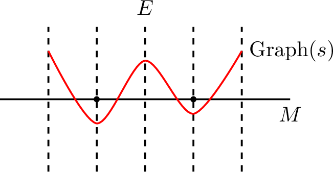