1 Introduction↩︎

Multi-agent systems have been extensively studied over the past 20 years. Initiated by early work such as [1], [2], although the roots can be found in much earlier work [3], it has become an active research area. But the realization that control systems often consist of many components with limited or restricted communication between them was already known much longer and studied in the area of decentralized control, see e.g. [4], [5]. Applications are for instance systems with many generators connected through a grid or traffic applications such as platoons of cars. The fallacy of early decentralized control is that it often created a specific agent which has a kind of supervisory role while other agents ensure communication to and from this supervisory agent. This approach turned out to be highly sensitive to failures in the network. Multi-agent systems created a different type of structure in these networks where all agents basically have a similar role towards achieving synchronization in the network. However, early work still heavily relied on knowledge of the network.

Later it was established that the protocols designed for a multi-agent systems would work for any network structure satisfying some underlying assumptions such as lower or upper bounds on the spectrum of the Laplacian matrix associated to the graph describing the network structure. In recent years, adaptive protocols were developed to achieve synchronization problem of MAS, see [6]–[9]. These protocols get rid of all assumptions on the network by using time-varying parameters in the protocol, related to these bounds on the eigenvalues of the Laplacian. However, it still requires that the network is strongly connected or has a direct spanning tree. This actually still inherently has some of the difficulties presented before. How can we check if this connectivity is present in the network? Secondly, what happens in case of a fault in the network that makes the network fail this assumption.

In the basic setup of a multi-agent system, the signals exchanged over the network converge to zero whenever the network synchronizes. So the fact that the network communication dies out over time is a weaker condition than output synchronization. We will refer to this weaker condition as network stability in this paper and a protocol achieving network stability achieves a form of weak synchronization as clarified in this paper.

It turns out that synchronization implies network stability and hence weak synchronization. But, more importantly, if the network has a directed spanning tree then the converse implication is true: weak synchronization implies classical synchronization.

We can therefore design adaptive nonlinear protocol which achieve weak state synchronization for any network without making any kind of assumptions. If the network happens to have a directed spanning tree then we obtain classical synchronization. However, if this is not the case then we describe in detail in this paper what kind of synchronization properties are preserved in the system. For applications this kind of weak synchronization yields what one would hope for. If the cars in a platoon lost connectivity between two subgroups because their distance has become too large the protocols will still achieve synchronization in both of these groups. If in a power system the connectivity between two subgroups is lost, each of these groups will internally achieve synchronization but, obviously, no global synchronization will be achieved. However, in general the decomposition of the network in a case of a fault might be more involved and these more general cases are also studied in the paper.

2 Communication network and graph↩︎

To describe the information flow among the agents we associate a weighted graph \(\mathcal{G}\) to the communication network. The weighted graph \(\mathcal{G}\) is defined by a triple \((\mathcal{V}, \mathcal{E}, \mathcal{A})\) where \(\mathcal{V}=\{1,\ldots, N\}\) is a node set, \(\mathcal{E}\) is a set of pairs of nodes indicating connections among nodes, and \(\mathcal{A}=[a_{ij}]\in \mathbb{R}^{N\times N}\) is the weighted adjacency matrix with non negative elements \(a_{ij}\). Each pair in \(\mathcal{E}\) is called an edge, where \(a_{ij}>0\) denotes an edge \((j,i)\in \mathcal{E}\) from node \(j\) to node \(i\) with weight \(a_{ij}\). Moreover, \(a_{ij}=0\) if there is no edge from node \(j\) to node \(i\). We assume there are no self-loops, i.e.we have \(a_{ii}=0\). A path from node \(i_1\) to \(i_k\) is a sequence of nodes \(\{i_1,\ldots, i_k\}\) such that \((i_j, i_{j+1})\in \mathcal{E}\) for \(j=1,\ldots, k-1\). A directed tree is a subgraph (subset of nodes and edges) in which every node has exactly one parent node except for one node, called the root, which has no parent node. A directed spanning tree is a subgraph which is a directed tree containing all the nodes of the original graph. If a directed spanning tree exists, the root of this spanning tree has a directed path to every other node in the network [10].

For a weighted graph \(\mathcal{G}\), the matrix \(L=[\ell_{ij}]\) with \[\ell_{ij}= { \setlength{\arraycolsep}{0.5mm}\left\{ \; \begin{array}{cl} \sum_{k=1}^{N} a_{ik}, & i=j,\\ -a_{ij}, & i\neq j, \end{array} \right.}\] is called the Laplacian matrix associated with the graph \(\mathcal{G}\). The Laplacian matrix \(L\) has all its eigenvalues in the closed right half plane and at least one eigenvalue at zero associated with right eigenvector \(\boldsymbol{1}\) [10]. The zero eigenvalues of Laplacian matrix is always semi simple, i.e. its algebraic and geometric multiplicities coincides. Moreover, the graph contains a directed spanning tree if and only if the Laplacian matrix \(L\) has a single eigenvalue at the origin and all other eigenvalues are located in the open right-half complex plane [11].

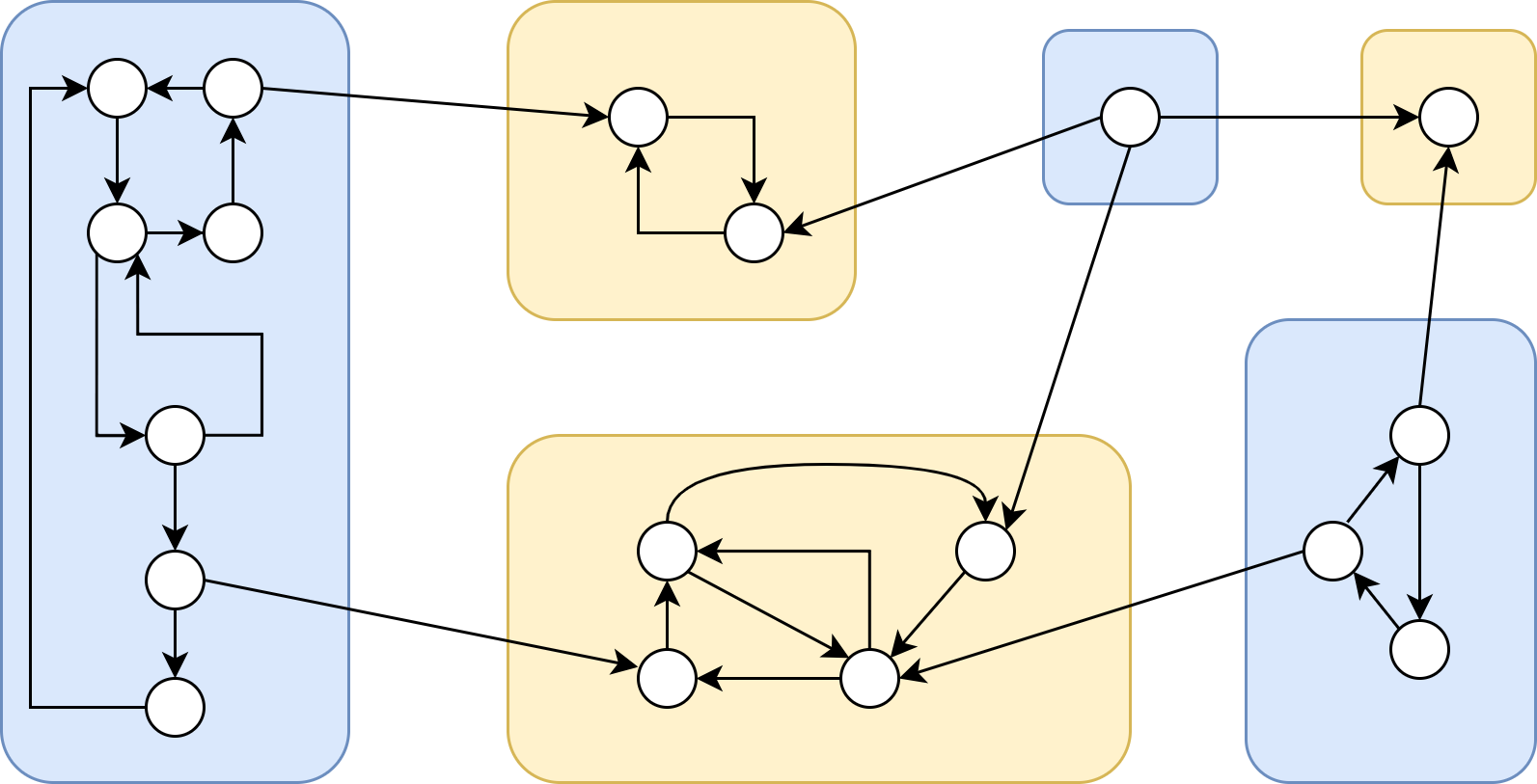
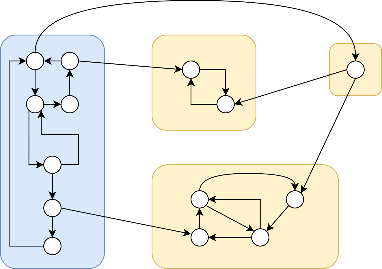
A directed communication network is said to be strongly connected if it contains a directed path from every node to every other node in the graph. For a given graph \(\mathcal{G}\) every maximal (by inclusion) strongly connected subgraph is called a bicomponent of the graph. A bicomponent without any incoming edges is called a basic bicomponent. Every graph has at least one basic bicomponent. A network has one unique basic bicomponent if and only if the network contains a directed spanning tree. In general, every node in a network can be reached by at least one basic bicomponent, see [12, p. 7]. In Fig. 1 a directed communication network with its bicomponents is shown. The network in this figure contains 6 bicomponents, 3 basic bicomponents (the blue ones) and 3 non-basic bicomponents (the yellow ones). In Fig. 2 a directed communication network with its bicomponents is shown. The network in this figure contains 4 bicomponents but only one basic bicomponent (the blue one).

In the absence of a directed spanning tree, the Laplacian matrix of the graph has an eigenvalue at the origin with a multiplicity \(k\) larger than \(1\). This implies that it is a \(k\)-reducible matrix and the graph has \(k\) basic bicomponents. The book [13] Definition 2.19 shows that, after a suitable permutation of the nodes, a Laplacian matrix with \(k\) basic bicomponents can be written in the following form: \[\label{Lstruc} L=\begin{pmatrix} L_0 & L_{01} & \cdots & \cdots & L_{0k} \\ 0 & L_1 & 0 & \cdots & 0 \\ \vdots & \ddots & \ddots & \ddots & \vdots \\ \vdots & & \ddots & L_{k-1} & 0 \\ 0 & \cdots & \cdots & 0 & L_k \end{pmatrix}\tag{1}\] where \(L_1,\ldots, L_k\) are the Laplacian matrices associated to the \(k\) basic bicomponents in our network. These matrices have a simple eigenvalue in \(0\) because they are associated with a strongly connected component. On the other hand, \(L_0\) contains all non-basic bicomponents and is a grounded Laplacian with all eigenvalues in the open right-half plane. After all, if \(L_0\) would be singular then the network would have an additional basic bicomponent.

3 Weak synchronization of MAS↩︎

In this section, we introduce the concept of weak synchronization for homogeneous MAS. Consider \(N\) homogeneous agents \[\label{system} \begin{system*}{cl} \dot{x}_i &= Ax_i +B u_i, \end{system*}\tag{2}\] where \(x_i\in\mathbb{R}^{n}\) and \(u_i\in\mathbb{R}^{m}\) are the state and input of agent \(i\) for \(i=1,\ldots, N\) with \((A,B)\) stabilizable and \((C,A)\) detectable.

The communication network provides agent \(i\) with the following information which is a linear combination of its own output relative to that of other agents \[\label{zeta1} \zeta_i=\sum_{j=1}^{N}a_{ij}(x_i-x_j),\tag{3}\] where \(a_{ij}\geqslant 0\) and \(a_{ii}=0\). The communication topology of the network can be described by a weighted and directed graph \(\mathcal{G}\) with nodes corresponding to the agents in the network and the weight of edges given by coefficient \(a_{ij}\). In terms of the coefficients of the associated Laplacian matrix \(L\), \(\zeta_i\) can be rewritten as \[\label{zeta} \zeta_i= \sum_{j=1}^{N}\ell_{ij}x_j.\tag{4}\] We denote by \(\mathbb{G}^N\) the set of all graphs with \(N\) nodes.

Our protocols are of the form: \[\label{protocoln} \begin{system*}{ccl} \dot{\xi}_i &=& f_i(\xi_i, \zeta_i) \\ u_i &=& g_i(\xi_i, \zeta_i) \end{system*}\tag{5}\]

In the following, we introduce the concept of network stability which is an intrinsically different concept compared to state synchronization.

Next, we present two lemmas to explain the difference between these two kind of synchronization

The proofs for Lemmas 1 and 2 are some minor adaptation of the proof of the same results in [14] to include nonlinear protocols.

4 Problem formulation↩︎

In this section, we consider the homogeneous agents of the form 2 with network communication given by 3 or, equivalently, 4 .

We make the following assumption.

Next, we define the problem addressed in this paper:

5 Protocol design for homogeneous MAS↩︎

We design an adaptive protocol to achieve the objectives of Problem 1 for this model 2 through two steps as following.

We have the following theorem.

Before we can proof the above theorem we derive two crucial lemmas.

We define \[x=\begin{pmatrix} x_1 \\ \vdots \\ x_N \end{pmatrix},\] and \[\rho=\begin{pmatrix} \rho_1 & 0 & \cdots & 0 \\ 0 & \rho_2 & \ddots & \vdots \\ \vdots & \ddots & \ddots & 0 \\ 0 & \cdots & 0 & \rho_N \end{pmatrix}\] We obtain \[\label{syscomp} \dot{x}=(I\otimes A)x-(\rho L\otimes BB^{\tiny T}P)x,\tag{8}\] and we define: \[\zeta_i = (L_i \otimes I)x,\] where \(L_i\) is the \(i\)’th row of \(L\) for \(i=1,\ldots, N\). We obtain \[\label{barxt3} \zeta = (L \otimes I) x.\tag{9}\] where \[\zeta=\begin{pmatrix} \zeta_1 \\ \vdots \\ \zeta_N \end{pmatrix}.\] By using 8 , we obtain \[\label{barxt4} \dot{\zeta} = (I\otimes A)\zeta -[L\rho \otimes BB^{\tiny T} P]\zeta.\tag{10}\] For any \(i\in \{1,\ldots, N\}\), from 10 we have that \[\dot{\zeta}_i = A\zeta_i -[L_i\rho \otimes BB^{\tiny T}P]\zeta.\] Define \[V_i = \zeta_i^{\tiny T}P \zeta_i,\] then we obtain \[\label{barxt7} \dot{V}_i = -\zeta_i^{\tiny T}\zeta_i + \zeta_i^{\tiny T}PBB^{\tiny T}P \zeta_i -2\zeta_i^{\tiny T}\left[ L_{i}\rho \otimes PBB^{\tiny T}P \right] \zeta.\tag{11}\] Since we know \[\dot{\rho}_i = r_i^{\tiny T}r_i\] where \[r_i = B^{\tiny T}P \zeta_i.\] we find that \(\rho_i\) bounded implies that \(r_i\in L_2\). Moreover, we have: \[\label{si} s_i =-2\left[ L_i \rho \otimes B^{\tiny T}P \right] \zeta = -2 \sum_{j=1}^N \ell_{ij} \rho_{j}r_j\tag{12}\] which yields \(s_i\in L_2\). We obtain from 11 that \[\label{barxt8} \dot{V}_i \leqslant-\eta V_i + r_i^{\tiny T}r_i + r_i^{\tiny T}s_i \leqslant-\eta V_i + 2r_i^{\tiny T}r_i + 2s_i^{\tiny T}s_i\tag{13}\] where \(\eta= \| P \|^{-1}\). Since \(r_i\) and \(s_i\) are both in \(L_2\) this implies \(V_i(t) \rightarrow 0\) which yields that \(\zeta_i(t)\rightarrow 0\). Since this is true for any \(i \in \{1,\ldots,N\}\) we find that we achieve weak state synchronization.

In the first Lemma we showed that if all the adaptive parameters remain bounded then we obtain our desired result. The next lemma establishes that the adaptive parameters are actually bounded and we can use Lemma 3 to establish synchronization.

Using the notation of Lemma 3 we obtain 8 . We first consider the case that some but not all of the \(\rho_i\) are unbounded. Without loss of generality, we renumber the agents such that \(\rho_i\) is unbounded for \(i\leqslant k\) while \(\rho_i\) is bounded for \(i>k\) with \(k<N\). We have \[\begin{gather} L = \begin{pmatrix} L_{11} & L_{12} \\ L_{21} & L_{22} \end{pmatrix},\quad x^k =\begin{pmatrix} x_1 \\ \vdots \\ x_k \end{pmatrix}, \quad x^k_c =\begin{pmatrix} x_{k+1} \\ \vdots \\ x_{N} \end{pmatrix},\\ \zeta^k =\begin{pmatrix} \zeta_{1} \\ \vdots \\ \zeta_{k} \end{pmatrix},\quad \zeta^k_c =\begin{pmatrix} \zeta_{k+1} \\ \vdots \\ \zeta_{N} \end{pmatrix}, \end{gather}\] with \(L_{11}\in \mathbb{R}^{k\times k}\). If all the agents associated to basic bicomponents have a bounded \(\rho_i\) this implies that agents associated to \(i=1,\ldots,k\) are not associated to basic bicomponents which implies that \(L_{11}\) is invertible. On the other hand, if the network is strongly connected we always have \(L_{11}\) is invertible since \(k<N\). We have \[\label{K1K2} \| v^k_c \|_2 < K_1.\tag{14}\] for suitably chosen \(K_1\) where \[v^k_c = (I \otimes B^{\tiny T}P) \zeta^k_c\] which follows from the fact that when \(\rho_i\) is bounded for \(i=k+1,\ldots, N\) then \(v_i\in L_2\) (note that \(\dot{\rho}_i = v_i^{\tiny T}v_i\)). We define \[\hat{x}^k= x^k+(L_{11}^{-1}L_{12}\otimes I) x^k_c.\] Using 8 we then obtain \[\label{barxt2xxx} \dot{\hat{x}}^k = (I\otimes A) \hat{x}^k -[\rho^{k} L_{11} \otimes BB^{\tiny T} P]\hat{x}^k -\left[L_{11}^{-1}L_{12}\rho^k_c \otimes B\right]v^k_c\tag{15}\] where \[\rho^k=\begin{pmatrix} \rho_1 & 0 & \cdots & 0 \\ 0 & \rho_2 & \ddots & \vdots \\ \vdots & \ddots & \ddots & 0 \\ 0 & \cdots & 0 & \rho_k \end{pmatrix}, \rho^k_c=\begin{pmatrix} \rho_{k+1} & 0 & \cdots & 0 \\ 0 & \rho_{k+2} & \ddots & \vdots \\ \vdots & \ddots & \ddots & 0 \\ 0 & \cdots & 0 & \rho_N \end{pmatrix}.\] Define \[\hat{v}^k =-(L_{11}^{-1}L_{12}\rho^k_c \otimes I)v^k_c ,\] then 14 in combination with the boundedness of \(\rho^k_c\) implies that there exists \(K_2\) such that \[\label{K3K4} \| \hat{v}^k \|_2 < K_2.\tag{16}\] We obtain \[\label{barxt2xxxy} \dot{\hat{x}}^k = (I\otimes A)\hat{x}^k -[\rho^k L_{11} \otimes BB^{\tiny T} P]\hat{x}^k+[I \otimes B]\hat{v}^k\tag{17}\] and we define: \[\label{Vj} V_k= (\hat{x}^k)^{\tiny T}(\rho^{-k} H^k \otimes P) \hat{x}^k,\tag{18}\] with \(\rho^{-k}=(\rho^k)^{-1}\) while: \[\label{HN} H^k=\begin{pmatrix} \alpha_1 & 0 & \cdots & 0 \\ 0 & \alpha_2 & \ddots & \vdots \\ \vdots & \ddots & \ddots & 0 \\ 0 & \cdots & 0 & \alpha_k \end{pmatrix}.\tag{19}\] By [15] we can choose \(\alpha_1,\ldots,\alpha_k>0\) such that \(H^k L_{11} +L_{11}^{\tiny T}H^k > 0\). It is easily seen that this implies that there exists a \(\gamma\) such that: \[\label{HkL11} H^kL_{11}+L_{11}^{\tiny T}H^k > 3\gamma L_{11}^{\tiny T}L_{11},\tag{20}\] We get from 17 that \[\begin{gather} \dot{V}_k \leqslant(\hat{x}^k)^{\tiny T}\left[ \rho^{-k} H^k \otimes (-I+PBB^{\tiny T}P) \right] \hat{x}^k\\ -(\hat{x}^k)^{\tiny T}\left[ (H^kL_{11}+L_{11}^{\tiny T}H^k) \otimes PBB^{\tiny T}P \right] \hat{x}^k \\ + 2(\hat{x}^k)^{\tiny T}\left[ \rho^{-k} H^k \otimes PB\right]\hat{v}^k. \end{gather}\] where we used that \(V_k\) is decreasing in \(\rho_i\) for \(i=1,\ldots, k\). The above yields for \(t>T\) that \[\begin{gather} \dot{V}_k \leqslant-V_k - 2\gamma (\hat{x}^k)^{\tiny T}\left[ L_{11}^{\tiny T}L_{11} \otimes PBB^{\tiny T}P \right] \hat{x}^k \\ + 2(\hat{x}^k)^{\tiny T}\left[\rho^{-k} H^k \otimes PB\right]\hat{v}^k, \end{gather}\] provided \(T\) is such that \[\rho^{-2k} (H^k)^2 < \gamma L_{11}^{\tiny T}L_{11},\] for \(t>T\) which is possible since we have \(\rho_i\rightarrow \infty\) for \(i=1,\ldots, k\). We define \[\check{v}^k = \left[ L_{11}^{-1} \rho^{-k}H^k \otimes I\right]\hat{v}^k.\] We get \[\label{lastone2xx} \dot{V}_k \leqslant- V_k - \gamma (\hat{x}^k)^{\tiny T}\left[ L_{11}^{\tiny T}L_{11} \otimes PBB^{\tiny T}P \right] \hat{x}^k +(\check{v}^k)^{\tiny T}\check{v}^k,\tag{21}\] for \(t>T\). Moreover, \[\label{rfgt} (\hat{x}^k)^{\tiny T}\left[ L_{11}^{\tiny T}L_{11} \otimes PBB^{\tiny T} P \right] \hat{x}^k \geqslant\sum_{i=1}^k \dot{\rho}_i,\tag{22}\] since \((L_{11}\otimes I)\hat{x}^k=\zeta^k\). Hence 21 implies \[\label{ttg1} \dot{V}_k \leqslant-V_k -\gamma \sum_{i=1}^k \dot{\rho}_{i} + (\check{v}^k)^{\tiny T}\check{v}^k\tag{23}\] Since the \(\rho_i\) are unbounded while \(\check{v}^k\in L_2\) this yields a contradiction since \(V_k\geqslant 0\).

Next we consider the case that all \(\rho_i\) are unbounded. In this case, we assumed the graph is strongly connected and hence by Lemma 5 presented in the appendix there exists \(\alpha_1,\ldots,\alpha_N>0\) such that ?? is satisfied with \(H^N\) given by 19 for \(k=N\). We define: \[\label{VN} V_N= x^{\tiny T}\left[ Q_{\rho} \otimes P \right] x,\tag{24}\] where \[\label{Qrho} Q_{\rho} = \rho^{-N} \left( H^N\rho^N - \mu_N \boldsymbol{h}_N\boldsymbol{h}_N^{\tiny T}\right) \rho^{-N}\tag{25}\] with \(\rho^{-N}=(\rho^N)^{-1}\), while \[\mu_N=\frac{1}{\sum_{i=1}^N \alpha_i\rho_i^{-1}},\qquad \boldsymbol{h}_N = \begin{pmatrix} \alpha_1 \\ \vdots \\ \alpha_N \end{pmatrix}.\] From Lemma 6 in the appendix we know that \(Q_{\rho}\) is decreasing in \(\rho_i\) for \(i=1,\ldots N\). Note that \(Q_\rho \rho L=H^N L\). We get from 8 that \[\begin{gather} \label{eqref} \dot{V}_N \leqslant x^{\tiny T}\left[ Q_\rho \otimes (-I+PBB^{\tiny T}P) \right] x\\ -x^{\tiny T}\left[ (H^NL+L^{\tiny T}H^N) \otimes PBB^{\tiny T}P \right] x \end{gather}\tag{26}\] It is easily verified that \(Q_{\rho}\boldsymbol{1}=0\). Moreover \(\mathop{\mathrm{Ker}}L = \mathop{\mathrm{span}}\{ \boldsymbol{1} \}\) since the network is strongly connected. Therefore \[\ker Q_{\rho} \subset \mathop{\mathrm{Ker}}L^{\tiny T}L\] Together with the fact that \(\rho_j\rightarrow \infty\) for \(j=1,\ldots, N\) and therefore \(Q_{\rho}\rightarrow 0\) this implies that there exists \(T\) such that \[\label{Qrhobound} Q_{\rho} < \gamma L^{\tiny T}L,\tag{27}\] is satisfied for \(t>T\).

The above together with ?? yields for \(t>T\) that \[\dot{V}_N \leqslant-\eta V_N - 2\gamma x^{\tiny T}\left[ L^{\tiny T}L \otimes PBB^{\tiny T}P \right] x\] where \(\eta=\| P\|^{-1}\). Note that \[x^{\tiny T}\left[ L^{\tiny T}L \otimes PBB^{\tiny T} P \right] x = \sum_{i=1}^N \dot{\rho}_i,\] The above implies \[\label{ttg1N} \dot{V}_N \leqslant-\eta V_N -\gamma \sum_{i=1}^N \dot{\rho}_{i}\tag{28}\] This again yields a contradiction since the \(\rho_i\) are unbounded while \(V_N \geqslant 0\).

The Laplacian matrix of the system in general has the form 1 . We note that if we look at the dynamics of the agents belonging to one of the basic bicomponents then these dynamics are not influenced by the other agents and hence can be analyzed independent of the rest of network. The network within one of the basic bicomponents is strongly connected and we can apply Lemmas 4 to guarantee that the \(\rho_i\) associated to a basic bicomponents are all bounded.

Next, we look at the full network again. We have already established that the \(\rho_i\) associated to all basic bicomponents are all bounded. Then we can again apply Lemmas 4 to conclude that the other \(\rho_i\) not associated to basic bicomponents are also bounded.

After having established that all the \(\rho_i\) are bounded, we can then apply Lemma 3 to conclude that we achieve scale-free weak state synchronization.

6 Numerical examples↩︎

In this section, we consider agent models of the form 2 with the following parameters, \[A=\begin{pmatrix} 0&1&0\\0&0&1\\0&0&0 \end{pmatrix},B=\begin{pmatrix} 0\\0\\1 \end{pmatrix}.\]

By using the protocol in 6 and 7 , we can obtain the following adaptive protocol:

6.1 Network containing a directed spanning tree↩︎

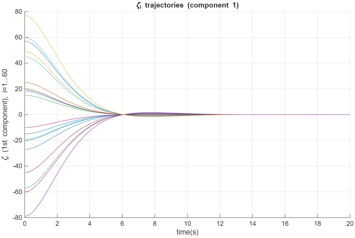
We consider state synchronization result for the 60-node homogeneous network shown in figure 3, which contains a directed spanning tree. By using the adaptive protocol 29 , we obtain \(\zeta_i\to 0\) and \(\dot{\rho}_i\) are bounded, which means state synchronization is achieved when the network contains a directed spanning tree, see Figs. 4 and 6.

6.2 Network without a directed spanning tree↩︎

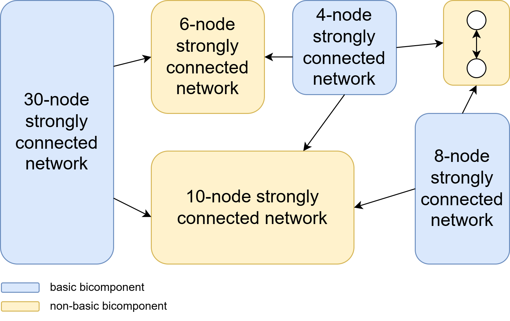
When some links have faults, the communication network might lose its directed spanning tree. For example, if two specific links are broken in the original 60-node network given by Figure 3, then we obtain the network as given in Figure 7

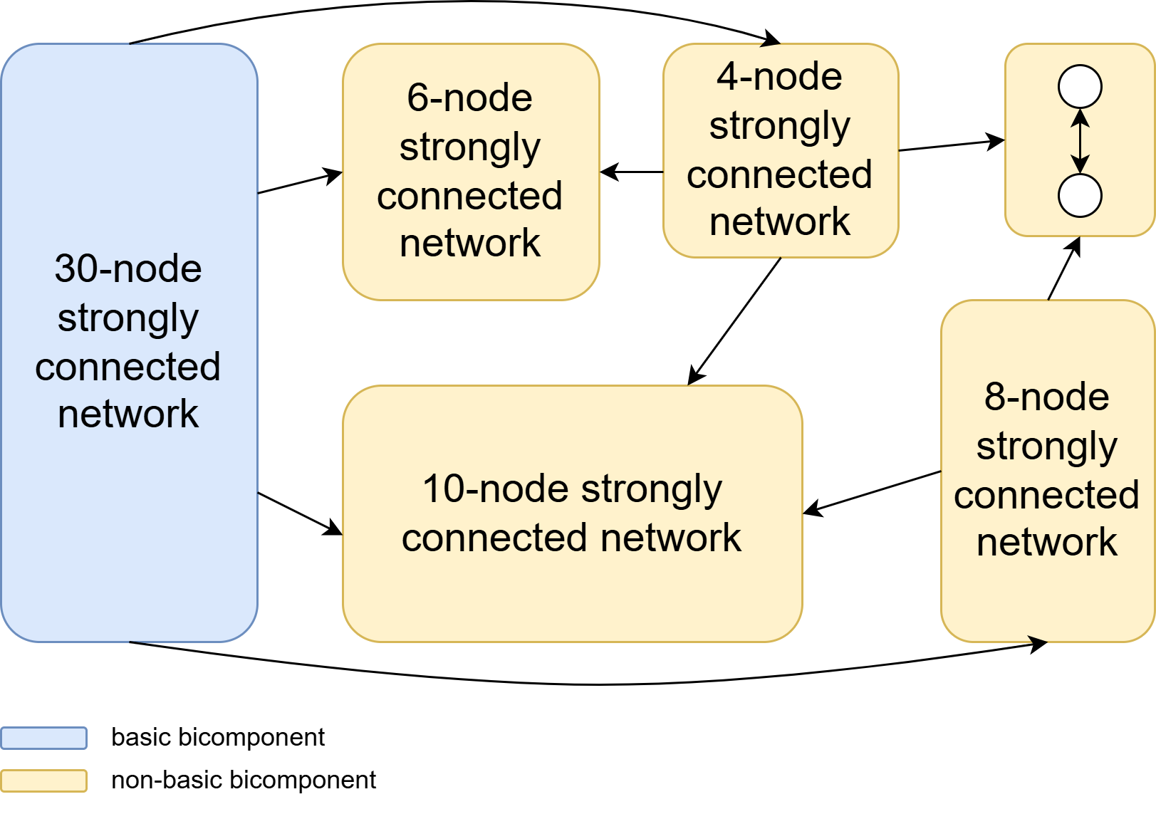
It is obvious that there is no spanning tree in Figure 7. We obtain three basic bicomponents (indicated in blue): one containing 30 nodes, one containing 8 nodes and one containing 4 nodes. Meanwhile, there are three non-basic bicomponents: one containing 10 nodes, one containing 6 nodes and one containing 10 nodes, which are indicated in yellow.

To show the proposed protocol can achieve the scale-free weak synchronization, we will provide 2 cases with 2 different graphs in this subsection.

6.2.1 Case I: 60-node graph shown in Fig. 7↩︎

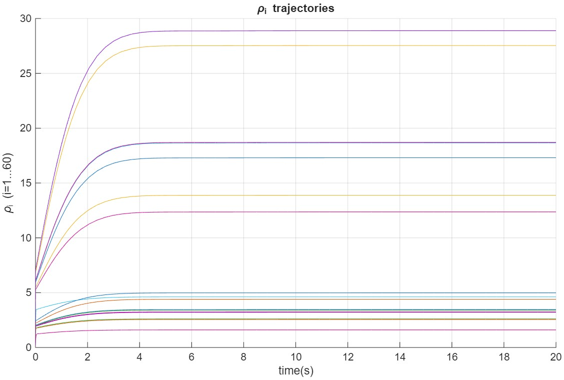
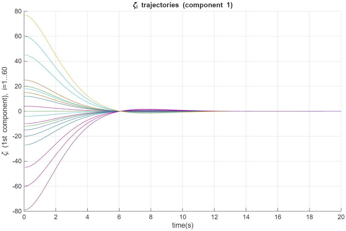
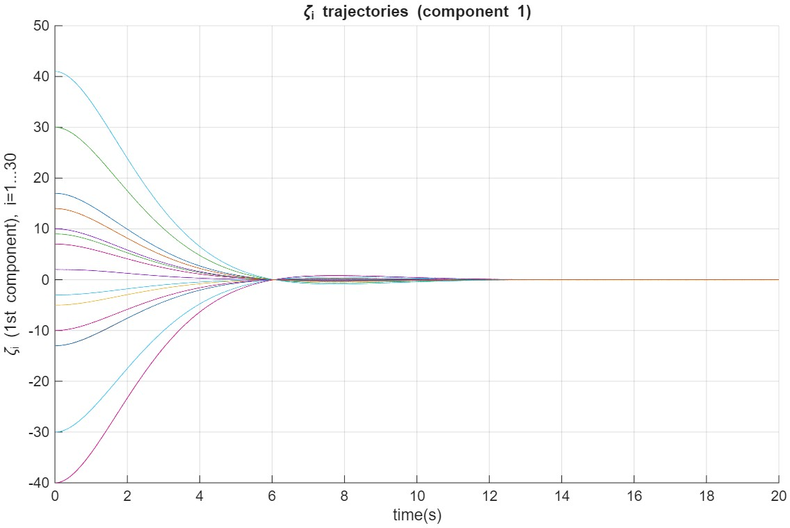
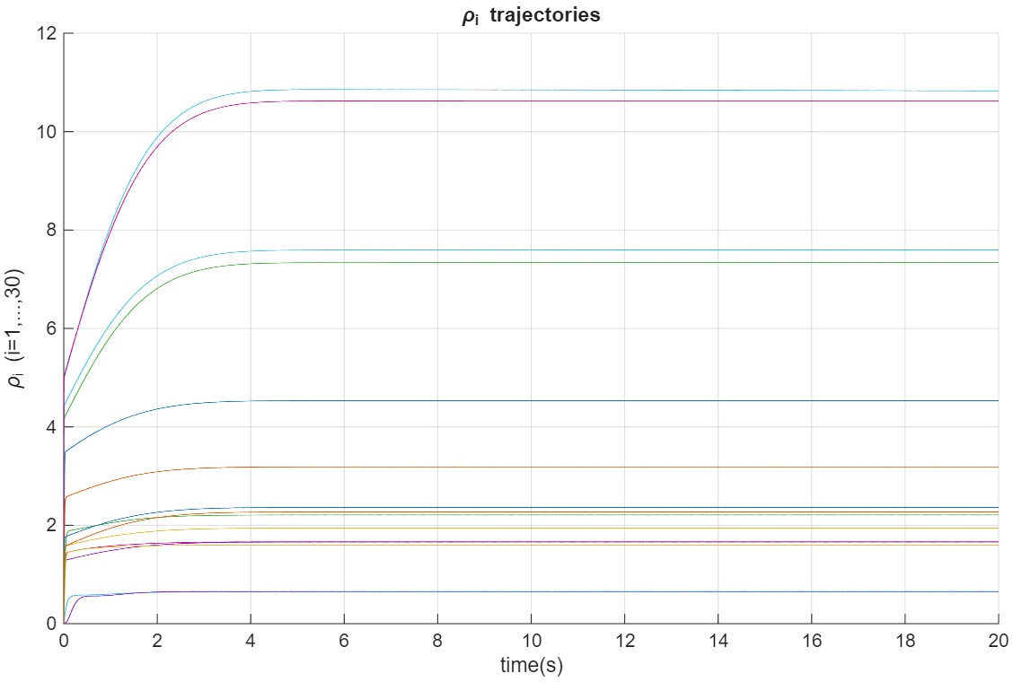
By using the adaptive protocol 29 , we obtain \(\zeta_i\to 0\) as \(t\to \infty\) for the graph shown in Fig. 7, which means weak synchronization is achieved in the absence of connectivity, see Fig. 8. And then, the adaptive parameters \(\rho_i\) are also bounded, see Fig. 9. It implies that the available network data for each agent goes to zero and the communication network becomes inactive.

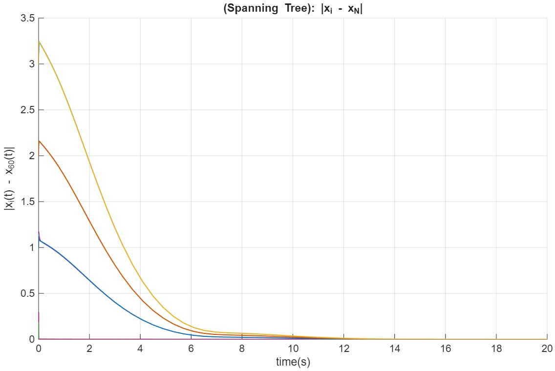
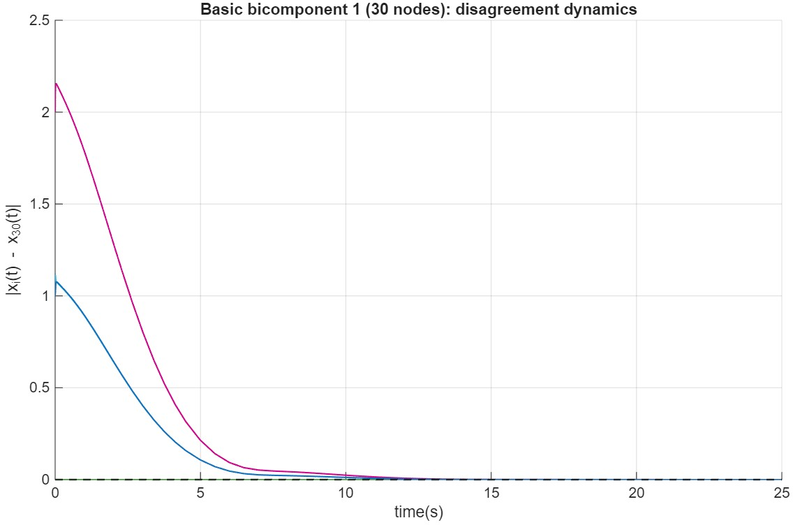
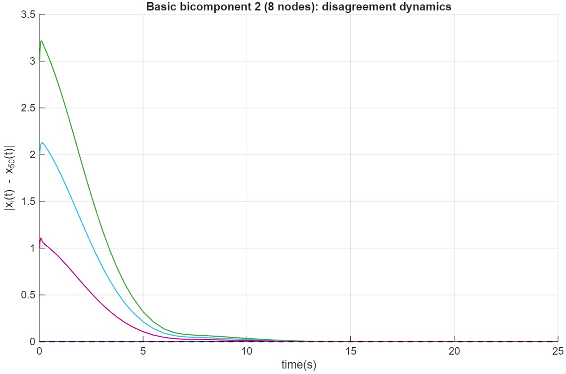
We have seen that for the 60-node network given in Figure 3 this adaptive protocol indeed achieves state synchronization. If we apply the same protocol to the network described by Figure 7 which does not contain a directed spanning tree, we again consider the six bicomponents constituting the network. We see that, consistent with the theory, we get state synchronization within the three basic bicomponents as illustrated in Figures 10, 11 and 12 respectively. Clearly, the disagreement dynamic among the agents (the errors between the state of agents) goes to zero within each basic bicomponent.

6.2.2 Case II: 30-node graph shown in Fig. 13↩︎

For the above 30-node graph, we obtain \(\zeta_i\to 0\) as \(t\to \infty\) for the graph shown in Fig. 13 by using the adaptive protocol 29 , i.e., weak synchronization is achieved in the absence of connectivity, see Fig. 14. And then, the adaptive parameters \(\rho_i\) are also bounded, see Fig. 15. It implies that the available network data for each agent goes to zero and the communication network becomes inactive.

Meanwhile, we obtain state synchronization within the three basic bicomponents as illustrated in Figures 16 and 17 respectively. Clearly, the disagreement dynamic among the agents (the errors between the state of agents) goes to zero within each basic bicomponent.

From these examples, we found that the protocol 29 can achieve the scale-free weak synchronization, which means that there exist \(\zeta_i\to 0\) as \(t\to \infty\) for any graph \(\mathscr{G}\in\mathbb{G}^N\) with arbitrary number of agents \(N\). And the common synchronization can be still achieved in the basic bicomponents of the graph.

7 Conclusion↩︎

In this paper we have introduced network stability and weak state synchronization for MAS and we have seen that this properties can be achieved via an adaptive nonlinear protocol. If we have a directed spanning tree then we obtain the classical concept of state synchronization. If, for instance due to a fault, the network no longer contains a directed spanning tree, then we still achieve network stability which implies a weaker form of synchronization, weak synchronization. Weak synchronizations guarantees a stable response to these faults: within basic bicomponents we still achieve synchronization and the states of agents not contained in a basic bicomponent converge to a convex combination of the asymptotic behavior achieved in the basic bicomponents.

Some useful lemmas↩︎

Choose a left eigenvector of the Laplacian \(L\) associated with eigenvalue \(0\): \[\begin{pmatrix} \alpha_1 & \cdots & \alpha_N \end{pmatrix} L =0\] Because the network is strongly connected, by [15] Theorem 4.31 we can choose \(\alpha_1,\ldots,\alpha_N>0\) and obtain: \[\label{app1} H^NL +L^{\tiny T}H^N \geqslant 0\tag{30}\] Note that \(H^N L\) has the structure of a Laplacian matrix with a zero row sum but also a zero column sum. The latter implies that \(L^{\tiny T}H^N\) also has the structure of a Laplacian matrix. The sum of two Laplacian matrices still has the structure of a Laplacian matrix. In other words, \(H^NL +L^{\tiny T}H^N\) has the structure of a Laplacian matrix. Note that this a undirected graph and there is an edge between nodes \(i\) and \(j\) if there is either an edge from node \(i\) to \(j\) or an edge from node \(j\) to \(i\) in the original graph associated with the Laplacian matrix \(L\). Since the graph associated with the Laplacian matrix \(L\) was strongly connected this implies that the graph associated with the Laplacian matrix \(H^NL +L^{\tiny T}H^N\) is also strongly connected. But then the rank of the matrix \(H^NL +L^{\tiny T}H^N\) is equal to \(N-1\) and hence we obtain: \[\label{app2} \mathop{\mathrm{Ker}}(H^NL +L^{\tiny T}H^N ) = \mathop{\mathrm{Ker}}L^{\tiny T}L = \mathop{\mathrm{span}}\{ \boldsymbol{1} \}\tag{31}\] 30 and 31 together imply that there exists a \(\gamma\) such that ?? is satisfied.

We also need to prove that the Lyapunov function in our paper is decreasing in \(\rho\) which is established in the following lemma:

Note that \[\label{appstar1} Q_{\rho} \boldsymbol{1} =0\tag{32}\] since \(\boldsymbol{h}_N^{\tiny T}\rho^{-N} \boldsymbol{1} = \mu_N^{-1}\). Define: \[z=\begin{pmatrix} z_1 \\ \vdots \\ z_N \end{pmatrix},\qquad \bar{z} =\begin{pmatrix} z_1-z_N \\ \vdots \\ z_{k-1}-z_N \end{pmatrix},\qquad \boldsymbol{h}_{N-1} =\begin{pmatrix} \alpha_1\\ \vdots \\ \alpha_{N-1}\end{pmatrix}\] and we find: \[V = \bar{z}^{\tiny T}(\rho^{N-1})^{-1} (\rho^{N-1}H^{N-1} - \mu_N \boldsymbol{h}_{N-1}\boldsymbol{h}_{N-1}^{\tiny T}) (\rho^{N-1})^{-1} \bar{z}\] using 32 . Some simple algebra establishes that: \[\begin{gather} (\rho^{N-1})^{-1} (\rho^{N-1}H^{N-1} - \mu_N \boldsymbol{h}_{N-1}\boldsymbol{h}_{N-1}^{\tiny T}) (\rho^{N-1})^{-1} \\= \left[ \rho^{N-1}(H^{N-1})^{-1} + \alpha_N^{-1}\rho_N \boldsymbol{1}_{N-1}\boldsymbol{1}_{N-1}^{\tiny T}\right]^{-1} \end{gather}\] and hence: \[V= \bar{z}^{\tiny T}\left[ \rho^{N-1}(H^{N-1})^{-1} + \alpha_N^{-1}\rho_N \boldsymbol{1}_{N-1}\boldsymbol{1}_{N-1}^{\tiny T}\right]^{-1} \bar{z}\] which clearly establishes that \(V\) is decreasing in \(\rho_i\) for \(i=1,\ldots, k\).

References↩︎