1 Introduction↩︎

The nonlinear schrödinger (NLS) equation and its vector form generalizations have been one of the most important research topics in the field of mathematical physics over the past fifty years. These equations have been derived in many physical fields, such as deep water waves, nonlinear optics, acoustics, and Bose–Einstein condensation( see e.g. [1]–[5] and references therein). Mathematically, both the NLS equations for scalars and vectors are completely integrable infinite-dimensional Hamiltonian systems, possessing extremely rich mathematical structures. It is well known that the initial value problem for these integrable systems can be solved using the inverse scattering transform (IST). The majority of IST literature on NLS systems has primarily focused on the case of zero boundary conditions (ZBCs)—where the potential decays to zero as the spatial variable tends to infinity. However, recent studies indicate that non-zero boundary conditions (NZBCs) are crucial for investigating modulation instability and the generation mechanisms of rogue waves (for example, see Refs. [6]–[9]). Consequently, research on the IST for NLS-type equations with non-zero backgrounds is increasing rapidly, and significant breakthroughs have been achieved in recent years. Next, we will briefly review the related research on this topic.

The IST for the defocusing scalar NLS equation with NZBCs was done as early as in [10], [11] and was recently revisited in [12]. Although the defocusing NLS equation does not admit soliton solutions on zero backgrounds, so-called dark/gray solitons were indeed found with NZBCs. The IST for the focusing NLS equation under NZBCs has recently been studied by Biondini et al. [13]. They provided a number of explicit solutions on a non-zero background, including soliton and breather solutions. Extending the IST from the scalar to the vector case requires additional considerations. Although the IST for the vector NLS equation with ZBCs was settled a long time ago [14], [15], the case with NZBCs, even for two-component systems (i.e., the Manakov system), has remained an open problem for nearly three decades. The inverse scattering analysis for the defocusing Manakov system with NZBCs was ultimately completed in Refs. [16], [17], where the authors utilized ideas originally introduced for solving the initial value problem of the three-wave interaction equations [18]. By constructing two new auxiliary eigenfunctions from the solutions of the adjoint spectral problem, it is ensured that the Jost solutions and the auxiliary solutions form a complete set, thereby enabling the derivation of a suitable Riemann-Hilbert (RH) problem. Soon after, the focusing Manakov system with NZBCs was studied in [19] using similar methods. Unfortunately, the approach used in [16], [17], [19] cannot be extended to the vector NLS equation with more than two components. Recently, Prinari et al. [20] have made a significant step towards the IST for the defocusing \(N\)-component NLS equation with NZBCs. However, several key issues remain open. A further IST characterization for the defocusing \(N\)-component NLS equation was presented in [21] for \(N=3\). These results were recently extended to the defocusing \(N\)-component (\(N \geq 4\)) [22] and the focusing \(N\)-component cases [23]. Regarding these advances, we suggest that readers refer to [24] to obtain a comprehensive review on this topic.

In the modern version of inverse scattering theory, the inverse problem is usually formulated as a RH problem. In the pioneering paper [25], Deift and Zhou introduced the nonlinear steepest descent method for oscillatory RH problems, thereby establishing the long-time asymptotic behavior of solutions to the modified KdV equation. Since then, the nonlinear steepest descent method and its extensions have become a fundamental tool for studying long-time asymptotics of integrable systems. The long-time asymptotic behavior of the defocusing and focusing scalar NLS equations on the zero background has been thoroughly studied  [26]–[31]. Meanwhile, there have been numerous studies on the long-time asymptotics for the focusing and defocusing scalar NLS equation with NZBCs [32]–[42]. In particular, in Ref. [40], Cuccagna and Jenkins investigated the asymptotic stability of dark solitons for the defocusing NLS equation using the \(\bar{\partial}\) steepest descent method. Our work was greatly motivated by their paper. Despite these advancements, the long-time asymptotics for vector NLS equation on a nonzero background remain unexplored. This is also an important open problem mentioned in Refs. [17], [21], [24].

This work is the first in a series of articles aimed at addressing this open problem, with a primary focus on the defocusing two-component case. The defocusing Manakov system is given by \[\label{E:demanakovS} \mathrm{i}\mathbf{q}_t +\mathbf{q}_{xx}+2(q_0^2 -\| \mathbf{q}\|) \mathbf{q}=0,\tag{1}\] where \(\mathbf{q}(x,t)\) is a two-component vector-valued function, i.e., \(\mathbf{q}=(q_1,q_2)^{\top}\). We will analyze the long-time behavior of solutions to system 1 satisfying the following boundary conditions: \[\label{E:bjtj} \lim_{x \to \pm \infty} \mathbf{q}(x,t)= \mathbf{q}_{\pm}=\mathbf{q}_c \mathrm{e}^{\mathrm{i}\theta_{\pm}},\tag{2}\] where \(\mathbf{q}_{\pm}\) is a constant two-component vector, (i.e., \(\mathbf{q}_{\pm}=(q_{1,\pm},q_{2,\pm})^{\top}\)), \(\|\cdot \|\) is the standard Euclidean norm, \(\mathbf{q}_c\) is a constant vector with norm \(q_0\), \(\theta_{\pm} \in [0,2 \pi)\), and subscripts \(x\) and \(t\) denote partial differentiation. Moreover, we assume that the convergence in 2 is sufficiently fast. Note that system 1 here differs from the classical Manakov equation [14] by an additional term \(2 q_0^2 \mathbf{q}\). One can remove this term by the simple rescaling \(\mathbf{q}(x,t) \to \mathbf{q}(x,t) \mathrm{e}^{-2\mathrm{i}q_0^2 t}\), and this term was added so that the boundary conditions 2 are independent of time. The boundary condition 2 is usually referred to as the parallel NZBCs, as \(\mathbf{q}_+=\mathbf{q}_- \mathrm{e}^{\mathrm{i}(\theta_+ - \theta_-)}\).

The strategy we employ to study the long-time behavior of the solutions to 1 \(-\)2 is to apply the Deift-Zhou steepest descent method to the RH problem derived in Ref. [17]. Although the corresponding Deift-Zhou analysis for the scalar case has been carried out by Cuccagna and Jenkins  [40]. However, as we will be seen, the Deift-Zhou analysis of the vecter case, like its inverse scattering analysis, presents new features and technical difficulties. We outline some of them below: \(\mathbf{(a)}\) The RH problem associated with 1 and 2 involves a \(3 \times 3\) matrix rather than a \(2 \times 2\) matrix. Additionally, it can be seen that the original jump matrix in Ref. [17] has an extremely complex structure (see [17]), which makes the triangular factorization extremely difficult to carry out. The key observation is that the symmetry properties of the reflection coefficients can be utilized to simplify the jump matrix, thereby obtaining the corresponding triangular factorization. \(\mathbf{(b)}\) The initial RH problem is singular at the origin. To ultimately transform it into a small-norm RH problem, it is necessary to remove this singularity. In the scalar case, there are two approaches to address this issue. The first method is to link the singular RH problem with a regular one and then applying the Deift-Zhou steepest descent method to the regular RH problem. This approach was initially proposed by Boutet et al. [43] to study the long-time asymptotic behavior of the modified Camassa Holm equation on a nonzero background, and it was subsequently applied within the framework of the defocusing scalar NLS equation [42], [44]. However, it is not easy to apply this method to our problem. The second method was developed by Cuccagna and Jenkins [40]. They observed that when the contribution of the discrete spectrum was removed, the corresponding \(\bar{\partial}\)-RH problem can be reduced to a pure \(\bar{\partial}\) problem (see [40]), with the singularity near the origin eliminated. Our approach is inspired by this idea; however,the analysis process has become more complicated due to the greater complexity of our RH problem. To finally obtain a small-norm RH problem, we right-multiply by \((\mathbf{M}^{out})^{-1}\) in the final transformation, where \(\mathbf{M}^{out}\) is the so-called outer parametrix defined by 46 . Although \((\mathbf{M}^{out})^{-1}\) has singularities at the branch points \(\pm q_0\), we will prove that the function after multiplication has no singularities at either the origin or the branch points. As a result, we obtain a small-norm RH problem, which enabled us to conduct error analysis. \(\mathbf{(c)}\) In order to perform the Deift-Zhou steepest descent analysis, it is necessary to find a suitable transformation that converts the jump matrix from an upper-lower triangular factorization to a lower-upper triangular factorization. We typically refer to this step as “conjugate" [45]. However, since the jump matrix is a \(3 \times 3\) one, this step is much more difficult than in the scalar case, which corresponds to a \(2 \times 2\) jump matrix. Furthermore, our case differs from other \(3 \times 3\) RH problems [46]–[49] whose jump matrices possess a block \(2 \times 2\) structure, thereby making it easier to complete the so-called ‘conjugate’ step. As one can see, our jump matrix (see 12 ) cannot be expressed in block form. We need to demonstrate how to complete the conjugation step for jump matrices of this type. It is worth noting that the transformation matrix we introduced contains the function \(\delta_1(z)\) (see Eq. 18 ). Since \(\ln \left(1-\frac{1}{\gamma(z)}|r_1(z)|^2-|r_2(z)|^2\right)\) generally blows up as \(z\) approaches the branch point \(q_0\), \(\delta_1(z)\) exhibits a singularity at \(q_0\). An analogous issue is encountered in the scalar case [40]. Our strategy is also analogous to that in Ref. [40]. By rewriting \(\delta_1(z)\) using the trace formula and combining it with the expression for \(\mathbf{M}\), one finds that although the transformation matrix \(\mathbf{\Delta}(z)\) is singular at \(q_0\), the transformed matrix \(\mathbf{M}^{(2)}\) remains bounded in the vicinity of the branch point \(q_0\). Therefore, this transformation will not bring about new difficulties. \(\mathbf{(d)}\) Finally, we would like to emphasize that the contour deformation process in this paper is fundamentally different from the scalar case [40], where the procedure to augment the jump contour is quite straightforward. From our perspective, the greater complexity of our contour deformation stems mainly from the fact that our jump matrix is \(3 \times 3\). In its triangular factorization, the upper or lower triangular matrix involves three phase functions with distinct properties. Consequently, we need to extend them off the real axis one by one based on their sign tables. On the contrary, in the scalar case, each triangular matrix contains only a single phase function, making the process considerably simple.

Moreover, we believe the methods presented in this paper can be applied to study the long-time behavior of the arbitrary \(N\)-component defocusing nonlinear Schrödinger equations with similar boundary conditions. Indeed, for the \(N\)-component case, the corresponding solutions have already been related to a block \(3 \times 3\) RH problem in Ref. [22]. Therefore, by employing this block matrix framework, the Deift-Zhou analysis developed in this work can be directly extended to the \(N\)-component scenario.

1.1 The preparation↩︎

\(\mathbf{Basic\;notations.}\) Throughout this paper, the asterisk indicates complex conjugation, and the superscripts \(\top\) and \(\dagger\) respectively represent the transpose and the conjugate transpose of the matrix. \(C>0\) and \(c>0\) will denote generic constants that may change within a computation. Let \({\mathbb{R}}_+=(0,+\infty)\), \({\mathbb{R}}_-=(-\infty,0)\), and let \(\mathbb{C}_+\) and \(\mathbb{C}_-\) represent the upper and lower complex half-planes, respectively. Let \(\bar{D}\) denote the closure of a region \(D\) in the complex plane.

To state our results, we need the following assumptions.

To define the asymptotic regions, we need to examine the velocities of the solitons. According to the results in Ref. [17], from the perspective of inverse scattering, the 1-soliton solution of system 1 with NZBCs 2 can be recovered from the scattering data \(\big\{ \zeta , \tau , r_1(z)=r_2(z)\equiv 0\big\}\), where \(\zeta\) denotes the discrete spectrum lying on the circle \(C_0\) with \(\mathop{ \mathrm{Im} }\nolimits\zeta >0\), \(\tau\) is the residue constant satisfying \(\frac{\tau}{\zeta} \in {\mathbb{R}}\), and \(\{ r_1, r_2\}\) represent the reflection coefficients (under our notation). By solving the pure soliton RH problem in Ref. [17], the 1-soliton solution can be given by the following explicit expression: \[\label{E:1soliton} \mathbf{q}^{[1]}_{sol}(x,t)=\mathbf{q}_+\left[1-\frac{\mathrm{i}\tau }{q_0} \left( \frac{\mathrm{e}^{\mathop{ \mathrm{Im} }\nolimits\zeta \left( -x+2t \mathop{ \mathrm{Re}}\nolimits\zeta \right) } }{1-\frac{\tau}{\zeta} (\frac{q_0}{2 \mathop{ \mathrm{Im} }\nolimits\zeta}) \mathrm{e}^{\mathop{ \mathrm{Im} }\nolimits\zeta \left( -x+2t \mathop{ \mathrm{Re}}\nolimits\zeta \right)} } \right) \right].\tag{3}\] From the above, we can observe that solitons have velocity \(v=2 \mathop{ \mathrm{Re}}\nolimits\zeta\). Let \(\xi=\frac{x}{2t}\). Since \(\mathop{ \mathrm{Re}}\nolimits\zeta<q_0\), we define the following three asymptotic sectors:

• The soliton region \(\mathcal{R}_{sol}\): \(\{(x,t)|\; |\xi|<q_0 \}\).

• The solitonless region: \(\{(x,t)|\; |\xi| >q_0 \}\).

• The transition region \(\{(x,t)|\; |\xi| \approx q_0 \}\). This region connects the soliton region and the solitonless region.

This paper primarily focuses on the asymptotic behavior within the soliton region, while the asymptotics in the remaining regions will be the subject of future work. It should be noted that the defined regions in our case is consistent with the definition in the scalar case. However, unlike in the scalar case, the sign of \(\xi\) will lead to different Deift-Zhou analyses. Therefore, we need to divide the soliton region into two parts and address them separately. Let us define the right half soliton region \(\mathcal{R}_{sol}^+\) and the left half soliton region \(\mathcal{R}_{sol}^-\) as follows: \[\mathcal{R}^+_{sol}=\{(x,t)|\;0<m_0<\xi<m_1 <q_0 \}, \quad \mathcal{R}^-_{sol}=\{(x,t): -m_1\leq \xi <-m_0 \},\] where the constants \(m_0\) and \(m_1\) are chosen without additional constraints. Our main theorem will provide the asymptotic formulas in these two regions, respectively. Let \(\mathcal{I}_+=[m_0,m_1]\) and \(\mathcal{I}_-=[-m_1,-m_0]\), then we have the following main results.

1.2 Main results↩︎

In fact, the above asymptotic formulas ?? and ?? can be further optimized. To illustrate this, we introduce the following notation: \[\begin{align} \mathcal{Z}(\mathcal{I}_{\pm})&=\{\zeta_j \;| \; \mathop{ \mathrm{Re}}\nolimits\zeta_j \in \mathcal{I}_{\pm} \},\quad N(\mathcal{I}_{\pm})=|\mathcal{Z}(\mathcal{I}_{\pm})|. \end{align}\] We observe that if \(\zeta_j \notin \mathcal{Z}(\mathcal{I}_{+})\), the contribution of the discrete spectrum \(\zeta_j\) to \(\mathbf{q}^{[N]}_{msol}(x,t)\) is exponentially small. Similarly, the contribution to \(\mathbf{\tilde{q}}^{[N]}_{msol}(x,t)\) from any \(\zeta_j \notin \mathcal{Z}(\mathcal{I}_{-})\) is also negligible. More precisely, we have the following result:

This paper is organized as follows. In section 2, we review the RH characterization of 1 and 2 . Sections 3 and 4 are devoted to the proof of Theorem 6 by employing the Deift-Zhou steepest descent method for the cases \(\xi \in \mathcal{I}_+\) and \(\xi \in \mathcal{I}_-\), respectively. In Section 5, we provide the proof of Theorem 7. Some technical proofs are presented in Appendices 7 to 9.

2 A Riemann-Hilbert formulation↩︎

In this section, we review the IST for the defocusing Manakov system [As:1] with the NZBCs 2 . Most of these results can be found in Ref. [17].

It is well-known that the defocusing Manakov system is completely integrable because it possesses a \(3\times 3\) matrix Lax pair [17]: \[\label{E:laxp1} \mathbf{\Phi}_x=\tilde{\mathbf{X}} \mathbf{\Phi}, \qquad \mathbf{\Phi}_t=\tilde{\mathbf{T}} \mathbf{\Phi},\tag{4}\] where \[\begin{align} &\tilde{\mathbf{X}}(x,t,k)=-\mathrm{i}k \mathbf{J}+\mathbf{Q}, \qquad \tilde{\mathbf{T}}(x,t,k)=2 \mathrm{i}k^2 \mathbf{J}- \mathrm{i}\mathbf{J}\left(\mathbf{Q}_x-\mathbf{Q}^2+q_0^2 \right)-2k \mathbf{Q},\\ &\mathbf{J}=\begin{pmatrix}1& \mathbf{0}^{\top}\\ \mathbf{0} &-\mathbf{I}_{2 \times 2} \end{pmatrix}, \quad \mathbf{Q}=\begin{pmatrix} 0& \mathbf{q}^{\dagger }\\ \mathbf{q}& \mathbf{0}_{2 \times 2} \end{pmatrix}. \end{align}\] It can be expected that when \(x \to \pm \infty\), the solutions to the scattering problem will approximate those of the asymptotic scattering problem \[\mathbf{\Phi}_x = \tilde{\mathbf{X}}_{\pm} \mathbf{\Phi}, \qquad \mathbf{\Phi}_t = \tilde{\mathbf{T}}_{\pm} \mathbf{\Phi},\] where \(\tilde{\mathbf{X}}_{\pm}= \lim_{x \to \pm \infty} \tilde{\mathbf{X}}\) and \(\tilde{\mathbf{T}}_{\pm}=\lim_{x \to \pm \infty} \tilde{\mathbf{T}}\). The eigenvalues of \(\tilde{\mathbf{X}}_{\pm}\) are \(\mathrm{i}k\) and \(\mathrm{i}\lambda\), where \[\label{E:lambda} \lambda(k) = \sqrt{k^2 - q^2_0}.\tag{5}\] Just as in the scalar case [40], these eigenvalues have branching phenomena. Following the approach in [17], we introduce a two-sheeted Riemann surface defined by 5 . The branch points occur at values of \(k\) where \(\lambda(k)=0\), namely \(k=\pm q_0\). We take the branch cut along \((-\infty, - q_0] \cup [q_0, \infty)\). Next, we introduce the uniformization variable by defining \[z=k+\lambda.\] The inverse transformation can be obtained by \[\begin{align} \label{E:intr} k = \frac{1}{2}(z + \frac{q^2_0}{z}),\quad \lambda = \frac{1}{2}(z - \frac{q^2_0}{z}). \end{align}\tag{6}\] Following the notation in Ref. [17], we denote the orthogonal vector of a two-component complex-valued vector \(\mathbf{v}=(v_1,v_2)\) as \(\mathbf{v}^{\perp}=\left(v_2,-v_1 \right)^{\dagger}\). We further introduce three matrices \[\label{E:trmatrix} \mathbf{E}_{\pm}(z)= \begin{pmatrix} 1&0&-\frac{\mathrm{i}q_0}{z}\\ \mathrm{i}\frac{\mathbf{q}_{\pm}}{z} & \frac{\mathbf{q}_{\pm}^{\perp}}{q_0}&\frac{\mathbf{q}_{\pm}}{q_0} \end{pmatrix}, \qquad \mathbf{\Lambda}(z)=\mathrm{diag} \left( -\lambda, k, \lambda \right),\qquad \mathbf{\Omega}(z)=\mathrm{diag} \left( -2k \lambda, k^2+\lambda^2, 2 k \lambda \right),\tag{7}\] which satisfy the relation \[\mathbf{E}_{\pm}^{-1} \tilde{\mathbf{X}}_{\pm} \mathbf{E}_{\pm}=\mathrm{i}\mathbf{\Lambda},\qquad \mathbf{E}_{\pm}^{-1} \tilde{\mathbf{T}}_{\pm} \mathbf{E}_{\pm}=-\mathrm{i}\mathbf{\Omega}.\] Then, it is easy to see that the Jost solutions \(\boldsymbol{\mu}_+(x,t,z)\) and \(\boldsymbol{\mu}_-(x,t,z)\) defined by the following integral equations are the unique solutions: \[\begin{align} &\boldsymbol{\mu}_-(x,t,z) = \mathbf{E}_-(z) + \int_{-\infty}^{x} \mathbf{E}_{-}(z) \mathrm{e}^{\mathrm{i}(x-y) \mathbf{\Lambda}(z)} \mathbf{E}^{-1}_{-}(z) \Delta \mathbf{Q}_{-}(y,t) \boldsymbol{\mu}_-(y,t,z) \mathrm{e}^{-\mathrm{i}(x-y) \mathbf{\Lambda}(z)} \mathrm{d}y, \tag{8}\\ &\boldsymbol{\mu}_+(x,t,z) = \mathbf{E}_+(z) - \int_{x}^{+\infty} \mathbf{E}_{+}(z) e^{\mathrm{i}(x-y) \mathbf{\Lambda}(z)} \mathbf{E}^{-1}_{+}(z) \Delta \mathbf{Q}_{+}(y,t) \boldsymbol{\mu}_+(y,t,z) \mathrm{e}^{-\mathrm{i}(x-y) \mathbf{\Lambda}(z)} \mathrm{d}y, \tag{9} \end{align}\] where \(\Delta \mathbf{Q}_{\pm}=\mathbf{Q}-\mathbf{Q}_{\pm}\) with \(\mathbf{Q}_{\pm}=\lim_{x \to \pm \infty} \mathbf{Q}(x,t)\). For a general potential where \(\Delta \mathbf{Q}_{\pm}\) decays suitably as \(x \to \pm \infty\), then it can be proved that \(\left\{ \boldsymbol{\mu}_{+1}, \boldsymbol{\mu}_{-3} \right\}\) and \(\left\{\boldsymbol{\mu}_{-1}, \boldsymbol{\mu}_{+3} \right \}\) are well-defined and continuous for \(z \in \bar{\mathbb{C}}_- \setminus \{0, \pm q_0\}\) and \(z \in \bar{\mathbb{C}}_+ \setminus \{0, \pm q_0\}\), respectively (see Theorem 2.1 in Ref. [17]). Moreover, these pairs of functions are analytic in \(\mathbb{C}_-\) and \(\mathbb{C}_+\), respectively. \(\mu_{\pm2}\) can only be defined on \({\mathbb{R}}\setminus \{0, \pm q_0\}\) and are nowhere analytic. However, since we let \(\Delta \mathbf{Q}_{\pm}(x,0)\equiv 0\) when \(|x|>L\) here, it follows from a similar analysis that \(\boldsymbol{\mu}_{\pm}(x,0,z)\) are well-defined and analytic for \(z \in \mathbb{C}\setminus \{0, \pm q_0\}\). In Ref. [17], the authors discussed the behavior of the Jost eigenfunctions at the branch points \(\pm q_0\). They have shown that the Jost solutions admit a well-defined limit at the branch points if \(\mathbf{q}\to \mathbf{q}_{\pm}\) sufficiently fast as \(z \to \pm q_0\).

We define \(\mathbf{\Phi}_{\pm}(x,t,z)=\boldsymbol{\mu}_{\pm}(x,t,z) \mathrm{e}^{\mathrm{i}\mathbf{\Lambda}(z)x - \mathrm{i}\mathbf{\Omega}(z)t}\). Then, \(\mathbf{\Phi}_{\pm}(x,t,z)\) are the fundamental solutions of Lax pair 4 for \(z \in {\mathbb{R}}\setminus \{0,\pm q_0 \}\). This is because \[\label{E:degamma} \mathrm{det} \boldsymbol{\mu}_{\pm}(x,t,z)=\mathrm{det} \mathbf{E}_{\pm}(z) =1-\frac{q_0^2}{z^2}:=\gamma(z).\tag{10}\] Therefore, there exists a matrix \(\mathbf{A}(z)\) independent of \(x\) and \(t\) such that \[\mathbf{\Phi}_-(x,t,z)=\mathbf{\Phi}_+(x,t,z) \mathbf{A}(z), \quad z \in {\mathbb{R}}\setminus \{0, \pm q_0 \}.\] According to Ref. [17], for general potentials \(\mathbf{q}(x,t)\) with suitably decaying \(\Delta \mathbf{Q}_{\pm}\) as \(x \to \pm \infty\), the \((11)\) and \((33)\) diagonal entries of \(\mathbf{A}(z)\), i.e., the analytic scattering coefficients, can be analytically extended to the upper and lower half-planes, respectively. However, in our case, since both \(\mathbf{\Phi}_-(x,0,z)\) and \(\mathbf{\Phi}_+(x,0,z)\) are analytic on \(\mathbb{C}\setminus \{0, \pm q_0\}\), it follows that \(\mathbf{A}(z)\) is well-defined and analytic on \(\mathbb{C}\setminus \{0, \pm q_0\}\). Defining \(\mathbf{B}(z) = \mathbf{A}^{-1}(z)\) , it is easy to see that \(\mathbf{B}(z)\) is also well-defined and analytic on \(\mathbb{C}\setminus \{0, \pm q_0\}\). Throughout the paper, we let \(a_{ij}\) and \(b_{ij}\) denote the \((ij)\)-th entries of the scattering matrices \(\mathbf{A}\) and \(\mathbf{B}\), respectively. We now present the properties of the scattering matrices \(\mathbf{A}(z)\) and \(\mathbf{B}(z)\), which are summarized from the results of Lemmas 2.13, 2.16 and subsections 2.6, 2.7 in Ref. [17].

Next, let us define the reflection coefficients \(r_{1}(z)\), \(r_2(z)\) and \(r_3(z)\) by \[\label{E:fsxsr12} r_1(z)=\frac{a_{21}(z)}{a_{11}(z)}, \quad r_2(z)=\frac{a_{31}(z)}{a_{11}(z)}, \quad r_{3}(z)=\frac{a_{23}(z)}{a_{33}(z)}.\tag{11}\] Due to symmetry ?? , it is straightforward to verify that \(r_1(z) =\frac{\mathrm{i}q_0}{z} r_3(\hat{z})\), where \(\hat{z}=\frac{q_0^2}{z}\). Therefore, it suffices to define only two reflection coefficients: \(r_1(z)\) and \(r_2(z)\). Since the scattering matrix elements \(a_{ij}(z)\) is analytic for \(z \in \mathbb{C}\setminus \{0,\pm q_0 \}\), the reflection coefficients \(r_1\) and \(r_2\) are also analytic on \(\mathbb{C}\setminus \{0,\pm q_0 \}\). The following lemma characterizes the properties of these three reflection coefficients.

As one can observe, the reflection coefficients we have defined are different from those in Ref [17]. This is because, according to our definition, the jump matrix of the associated RH problem can be expressed in a more concise form. Indeed, the jump matrix appearing in [17] is extremely complex, which makes it difficult to perform a triangular decomposition. However, by utilizing ?? and ?? , we demonstrate that this jump matrix can actually be expressed in the following form: \[\label{E:Vex} \mathbf{V}(x,t,z)=\mathrm{e}^{\Theta(x,t,z)} \begin{pmatrix} 1-\frac{1}{\gamma(z)}|r_1(z)|^2-|r_2(z)|^2& \frac{1}{\gamma(z)}(-r_1(z)+r_2(z)r_3(z))^*& -r^*_2(z) \\ r_1(z)-r_2(z)r_3(z) &1+\frac{1}{\gamma(z)}|r_3(z)|^2& -r_3(z)\\ r_2(z) & -\frac{1}{\gamma(z)}r_3^*(z)& 1 \end{pmatrix} \mathrm{e}^{-\Theta(x,t,z)},\tag{12}\] where \(\Theta(x,t,z)=\mathrm{diag}\left(\theta_1(x,t,z),\theta_2(x,t,z),\theta_3(x,t,z) \right)\) with \[\label{E:theta123} \begin{cases} \theta_1(x,t,z)= -\mathrm{i}\lambda(z)x+2 \mathrm{i}k(z) \lambda(z) t,\\ \theta_2(x,t,z)=\mathrm{i}k(z)x-\mathrm{i}(k^2(z)+\lambda^2(z))t,\\ \theta_3(x,t,z)=\mathrm{i}\lambda(z)x-2 \mathrm{i}k(z) \lambda(z) t. \end{cases}\tag{13}\] The derivation of 12 is provided in Appendix 7.2.

Following the idea from Ref. [17], we define a piecewise meromorphic function \(\mathbf{M}(x,t,z)\) as follows (see [17]): \[\label{E:exM} \mathbf{M}(x,t,z)=\begin{cases} \left(\frac{\boldsymbol{\mu}_{-1}}{a_{11}}, \frac{\mathbf{m}}{b_{33}}, \boldsymbol{\mu}_{+3} \right), & \mathrm{Im} z >0,\\ \left(\boldsymbol{\mu}_{+1}, -\frac{\bar{\mathbf{m}} }{b_{11}}, \frac{\boldsymbol{\mu}_{-3}}{a_{33}} \right), & \mathrm{Im} z <0, \end{cases}\tag{14}\] where \(\bar{\mathbf{m}}(x,t,z)=-\mathbf{J}[\mathbf{\Phi}_{-1}^* \times \mathbf{\Phi}_{+3}^*] (x,t,z^*) / \gamma(z),\; \mathbf{m}(x,t,z)=-\mathbf{J}[\mathbf{\Phi}_{-3}^* \times \mathbf{\Phi}_{+1}^*] (x,t,z^*) / \gamma(z)\). Here \(``\times"\) denotes the usual cross product. Then, according to the results in Ref. [17], one can conclude that \(\mathbf{M}(x,t,z)\) satisfies the following RH problem:

For the self-consistency of this paper, we establish the uniqueness of the solution to the above RH problem.

Therefore, \(\mathbf{M}(x,t,z)\) defined by 14 is the unique solution to RH problem 13. Combined with the asymptotic behavior of \(\mathbf{M}(x,t,z)\) as \(z \to \infty\) (see [17]), we summarize the following reconstruction theorem:

In the following sections, we will perform the Deift-Zhou steepest descent analysis on RH problem 13, thereby obtaining the long-time asymptotics of the potential \(\mathbf{q}(x,t)\) through reconstruction formula ?? .

3 Long-time asymptotics in \(\mathcal{R}^{+}_{sol}\)↩︎

In this section, we will investigate asymptotics of the RH problem 13 as \(t \to \infty\) by using Deift–Zhou nonlinear steepest descent method [25]. The main idea is to convert the original RH problem into a small-norm one via a series of explicit and invertible transformations. Throughout this section, it is assumed that \(\xi=x/(2t)\) in the compact subset \(\mathcal{I}_+\) of \((0,q_0)\).

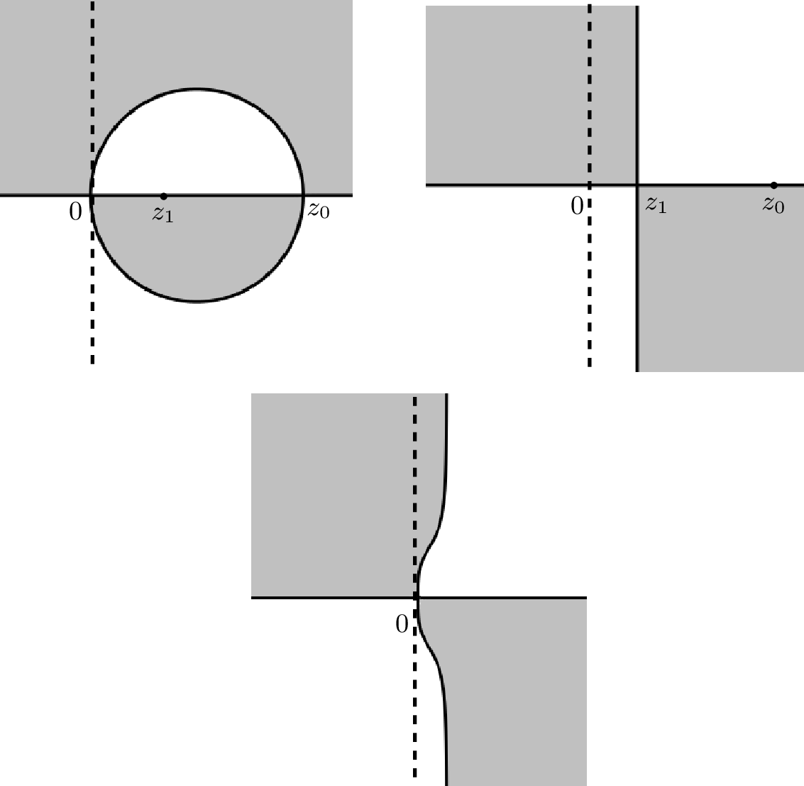
We define the phase functions \(\phi_{i j}(\xi,z)\) by \(\theta_{i j}(x,t,z)=t\phi_{i j}(\xi,z)\), \(1\leq i,j \leq 3\), which originate from the oscillatory exponential terms in the jump matrix \(\mathbf{V}\). Let’s consider the following three phase functions: \[\phi_{32}(\xi,z)=-2 \mathrm{i}\xi \frac{q_0^2}{z}+\mathrm{i}\frac{q_0^4}{z^2}, \quad \phi_{21}(\xi,z)=2 \mathrm{i}\xi z-\mathrm{i}z^2, \quad \phi_{31}(\xi,z)=4 \mathrm{i}\xi \lambda(z)-4 \mathrm{i}k(z)\lambda(z).\] Set \(z_1=\xi\) and \(z_0=\frac{q_0^2}{\xi}\), then \(z_0\) is the unique saddle point of \(\phi_{32}(\xi,k)\), \(z_1\) is the unique saddle point of \(\phi_{21}(\xi,k)\), and the function \(\phi_{31}(\xi,k)\) has no saddle point on \({\mathbb{R}}\). The signature tables for \(\mathop{ \mathrm{Re}}\nolimits\phi_{21}(\xi,k)\), \(\mathop{ \mathrm{Re}}\nolimits\phi_{32}(\xi,k)\) and \(\mathop{ \mathrm{Re}}\nolimits\phi_{31}(\xi,k)\) are shown in Fig. 1.

3.1 The transformation: \(\mathbf{M}\to \mathbf{M}^{(1)}\)↩︎

Lemma 1 shows that as \(z \to 0\) within the region \(S_d\), the limits of \(\{r_j(z) \}_{j=1}^3\) exist. This indicates that our augmented contour near zero should be chosen within \(S_d\). More precisely, we define the contour \(\Sigma^{(1)}\) as \[\begin{align} \Sigma^{(1)}_2&=\left \{ z:\;(\mathop{ \mathrm{Re}}\nolimits z)^2+(\mathop{ \mathrm{Im} }\nolimits z -1/2)^2=1/4, \;\; - \sqrt{|\varepsilon ^2-\varepsilon |}\leq \mathop{ \mathrm{Re}}\nolimits z \leq 0, \;\; 0\leq \mathop{ \mathrm{Im} }\nolimits z \leq \varepsilon \right \} \\ &\cup \left \{ z: s + \mathrm{i}\varepsilon, \;s \leq - \sqrt{|\varepsilon ^2-\varepsilon |} \right\} , \qquad \Sigma^{(1)}_1={\mathbb{R}}_+=(0,+\infty), \\ \Sigma^{(1)}_4&=\left \{ z: (\mathop{ \mathrm{Re}}\nolimits z)^2+(\mathop{ \mathrm{Im} }\nolimits z +1/2)^2=1/4, \;\;- \sqrt{|\varepsilon ^2-\varepsilon |}\leq \mathop{ \mathrm{Re}}\nolimits z \leq 0, \;\; -\varepsilon \leq \mathop{ \mathrm{Im} }\nolimits z \leq 0 \right \} \\ &\cup \left \{ z: s -\mathrm{i}\varepsilon , \;s \leq - \sqrt{|\varepsilon ^2-\varepsilon |} \right\}, \qquad \Sigma^{(1)}_3={\mathbb{R}}_-=(-\infty,0). \end{align}\] The contour \(\Sigma^{(1)}\) is oriented as shown in Fig. 2. It is easy to see that the contour \(\Sigma^{(1)}\) lies within the strip region \(S_{\varepsilon }=\{z:\;\mathop{ \mathrm{Im} }\nolimits z \leq \varepsilon \}\) . We choose \(\varepsilon\) sufficiently small so that the strip region \(S_{\varepsilon }\) contains no discrete spectrum.

The purpose of the first transformation is to extend the jump matrix off the negative real axis. One can directly verify that the jump matrix \(\mathbf{V}(x,t,z)\) admits the following decomposition on \(z \in {\mathbb{R}}\): \[\label{E:sjfjV} \mathbf{V}=\mathrm{e}^{\Theta} \begin{pmatrix} 1 & -\frac{1}{\gamma} r_1^* & -r_2^* \\ 0 & 1 & -r_3\\ 0 & 0 &1 \end{pmatrix} \begin{pmatrix} 1 & 0 & 0\\ r_1&1 &0 \\ r_2& -\frac{1}{\gamma}r_3^* &1 \end{pmatrix} \mathrm{e}^{-\Theta}=\mathbf{V}^{U} \mathbf{V}^L,\tag{15}\] where \[\label{E:VUL} \begin{align} \mathbf{V}^U=\mathrm{e}^{\Theta} \begin{pmatrix} 1 & -\frac{1}{\gamma(z)} r_{1}^*(z^*) & -r_{2}^*(z^*)\\ 0 & 1 & -r_{3}(z)\\ 0& 0 &1 \end{pmatrix} \mathrm{e}^{-\Theta}, \quad \mathbf{V}^L= \mathrm{e}^{\Theta} \begin{pmatrix} 1 & 0&0\\ r_{1}(z) & 1 & 0\\ r_{2}(z)& -\frac{1}{\gamma(z)}r_{3}^*(z^*) &1 \end{pmatrix} \mathrm{e}^{-\Theta}. \end{align}\tag{16}\] We define the matrix \(\mathbf{G}(x,t,z)\) as follows: \[\label{E:G} \mathbf{G}(x,t,z)= \begin{cases} \big( \mathbf{V}^{L} \big)^{-1}(x,t,z), & z \in \mathcal{R}_1,\\ \mathbf{V}^{U}(x,t,z), & z \in \mathcal{R}_2,\\ \mathbf{I}, & \text{elsewhere.} \end{cases}\tag{17}\] The regions \(\{\mathcal{R}\}_{j=1}^2\) are as shown in Fig. 2. Our first transformation is defined as \(\mathbf{M}^{(1)}=\mathbf{M}\mathbf{G}\). Then the jump contour associated with \(\mathbf{M}^{(1)}\) is \(\Sigma^{(1)}\)(see Fig. 2 ). The jump matrix is given by \(\mathbf{V}^{(1)}=\mathbf{G}_-^{-1}\mathbf{V}\mathbf{G}_+\). A straightforward calculation yields \[\begin{align} \mathbf{V}^{(1)}_1=\mathbf{V}, \quad \mathbf{V}^{(1)}_2= \mathbf{V}^{L}, \quad \mathbf{V}^{(1)}_3=\mathbf{I}, \quad \mathbf{V}^{(1)}_4=\mathbf{V}^U. \end{align}\] Here, \(\mathbf{V}^{(1)}_j\) denotes the jump matrix \(\mathbf{V}^{(1)}\) restricted to \(\Sigma^{(1)}_j\). In the following sections, we will adhere to this notational convention.

3.2 The transformation: \(\mathbf{M}^{(1)} \to \mathbf{M}^{(2)}\)↩︎

From Fig. 1, one can observe that the upper-lower triangular factorization 15 is no longer appropriate on the positive real axis \({\mathbb{R}}_+\). The purpose of our second transformation is to convert the jump on \({\mathbb{R}}_+\) from an upper-lower triangular factorization to a lower-upper triangular factorization. To this end, we define a diagonal matrix \(\mathbf{\Delta}(z)=\mathrm{diag} \left( \delta_1(z), \delta_2(z), \delta_3(z) \right)\), where \(\delta_1(z)\), \(\delta_2(z)\) and \(\delta_3(z)\) are to be determined, and they are analytic on \(\mathbb{C}\setminus {\mathbb{R}}_+\) and have jumps on \({\mathbb{R}}_+\). Let us examine what conditions should be imposed on \(\{\delta_j \}_{j=1}^3\) such that \(\mathbf{\Delta}_-^{-1}\mathbf{V}^{(1)} \mathbf{\Delta}_+\) admits a lower-upper triangular factorization. Firstly, we define \(\delta_1(z)\) for \(z \in \mathbb{C}\setminus {\mathbb{R}}_+\) by \[\label{E:soldel1} \delta_1(z)=\mathrm{exp}\bigg \{-\frac{1}{2 \pi \mathrm{i}} \int_{{\mathbb{R}}_+} \frac{\ln \left(1-\frac{1}{\gamma(s)}|r_1(s)|^2-|r_2(s)|^2\right)}{s-z} \mathrm{d}s \bigg\}.\tag{18}\] Using the symmetry satisfied by \(\mathbf{A}(z)\) and \(\mathbf{B}(z)\) (see ?? and ?? ), one can easily verify that \[\left(1-\frac{1}{\gamma(z)}|r_1(z)|^2-|r_2(z)|^2\right)^{-1}=a_{11}(z) b_{11}(z) =a_{11}(z) a^*_{11}(z), \quad z \in {\mathbb{R}}_+ \setminus \{ q_0\}.\] Although \(a_{11}(z)\) blows up as \(z \to q_0\), the function \(\delta_1(z)\) is nevertheless well-defined for \(z \in \mathbb{C}\setminus [0,+\infty)\), due to the fact that \(\|\ln (|a_{11}(\cdot)|^2) \|_{L^{1}({\mathbb{R}}_+)} < \infty\). Based on the asymptotic behavior of \(a_{11}(z)\) as \(z \to 0\) and \(z \to q_0\), and that of \(r_1(z)\) and \(r_2(z)\) as \(z \to \infty\), it’s easy to show that \(\|\ln (|a_{11}(\cdot)|^2) \|_{L^{1}({\mathbb{R}}_+)} < \infty\) . Furthermore, we have the following lemma.

We still leave \(\delta_2(z)\) and \(\delta_3(z)\) undetermined, and we will now derive the jump conditions that \(\delta_2\) and \(\delta_3\) should satisfy. Let \(r_4=r_1(z)-r_2(z)r_3(z)\). Firstly, \(\mathbf{\Delta}_-^{-1}\mathbf{V}^{(1)} \mathbf{\Delta}_+\) can be expressed as \[\label{E:zuV2} \mathbf{\Delta}_-^{-1}\mathbf{V}^{(1)} \mathbf{\Delta}_+ = \mathrm{e}^{\Theta} \begin{pmatrix} 1 & -\frac{1}{\gamma}r^*_4 \frac{\delta_{2+} }{\delta_{1-}}& -r_2^* \frac{\delta_{3+}}{\delta_{1-}}\\ r_4 \frac{\delta_{1+}}{\delta_{2-}} &(1+ \frac{1}{\gamma}|r_3|^2)\frac{\delta_{2+}}{\delta_{2-}}& -r_3 \frac{\delta_{3+}}{\delta_{2-}}\\ r_2 \frac{\delta_{1+}}{\delta_{3-}}& -\frac{1}{\gamma}r_3^* \frac{\delta_{2+}}{\delta_{3-}}& \frac{\delta_{3+}}{\delta_{3-}} \end{pmatrix} \mathrm{e}^{-\Theta}.\tag{20}\] We observe that if \(\mathbf{\Delta}_-^{-1}\mathbf{V}^{(1)} \mathbf{\Delta}_+\) has lower-upper triangular factorization, it must be in the following form : \[\label{E:fjV2} \mathbf{\Delta}_-^{-1}\mathbf{V}^{(1)} \mathbf{\Delta}_+ = \mathrm{e}^{\Theta} \begin{pmatrix} 1 &0&0\\ r_4 \frac{\delta_{1+}}{\delta_{2-}} &1&0\\ r_2 \frac{\delta_{1+}}{\delta_{3-}}& A_1 \frac{\delta_{2+}}{\delta_{3-}}& 1 \end{pmatrix} \begin{pmatrix} 1 & -\frac{1}{\gamma}r^*_4 \frac{\delta_{2+}}{\delta_{1-}}& -r_2^* \frac{\delta_{3+}}{\delta_{1-}}\\ 0 &1&B_1 \frac{\delta_{3+}}{\delta_{2-}}\\ 0&0& 1 \end{pmatrix} \mathrm{e}^{-\Theta},\tag{21}\] where \(A_1\) and \(B_1\) are to be determined. Equating the right-hand sides of 20 and 21 yields the following four equations: \[\label{E:sfc} \begin{align} 1-\frac{1}{\gamma}|r_4|^2\frac{\delta_{1+}}{\delta_{1-}}\frac{\delta_{2+}}{\delta_{2-}}=(1+\frac{1}{\gamma}|r_3|^2)\frac{\delta_{2+}}{\delta_{2-}},&\\ A_1\frac{\delta_{2+}}{\delta_{3-}}-\frac{1}{\gamma}r_2 r_4^* \frac{\delta_{1+}}{\delta_{1-}}\frac{\delta_{2+}}{\delta_{3-}}=- \frac{1}{\gamma}r_3^*\frac{\delta_{2+}}{\delta_{3-}}, &\\ B_1 \frac{\delta_{3+}}{\delta_{2-}}- r_2^*r_4\frac{\delta_{1+}}{\delta_{1-}}\frac{\delta_{3+}}{\delta_{2-}}=-r_3\frac{\delta_{3+}}{\delta_{2-}}, & \\ 1+A_1 \;B_1 \frac{\delta_{2+}}{\delta_{2-}}\frac{\delta_{3+}}{\delta_{3-}}-|r_2|^2\frac{\delta_{1+}}{\delta_{1-}}\frac{\delta_{2+}}{\delta_{3-}} = \frac{\delta_{3+}}{\delta_{3-}}. & \end{align}\tag{22}\] By using the symmetries of the scattering matrices \(\mathbf{A}(z)\) and \(\mathbf{B}(z)\) (see ?? and ?? ) to simplify the system, we obtain that \(\{\delta_j\}_{j=1}^3\) should satisfy the following jump conditions: \[\label{E:deltaju} \begin{align} \mathbf{\Delta}_+(z)=\mathbf{\Delta}_-(z) \begin{pmatrix} a_{11}(z) b_{11}(z)& & \\ & \frac{a_{33}(z) b_{33}(z)}{a_{11}(z) b_{11}(z)} & \\ & & \frac{1}{a_{33}(z) b_{33}(z)} \end{pmatrix}, \qquad \; z \in {\mathbb{R}}_+ \setminus \{q_0\}, \end{align}\tag{23}\] and we have \[\begin{align} B_1(z)=-r_3(z)+r_4(z) r_2^*(z)a_{11}(z) b_{11}(z), \qquad A_1(z)=\frac{1}{\gamma(z)}B_1^*(z), \qquad z\in {\mathbb{R}}_+ \setminus \{q_0\}. \end{align}\] A natural choice satisfying jump conditions 23 is \[\label{E:Deldef} \mathbf{\Delta}(z)= \begin{pmatrix} \delta_1(z) & & \\ &\frac{1}{\delta_1(z) \delta_1(\hat{z})} & \\ & & \delta_1(\hat{z}) \end{pmatrix},\tag{24}\] where \(\hat{z}=\frac{q_0^2}{z}\). In other words, if we let \(\mathbf{\Delta}(z)\) be defined by 24 , then \(\mathbf{\Delta}_-^{-1}\mathbf{V}^{(1)} \mathbf{\Delta}_+\) admits a lower-upper triangular factorization. It should be noted that \(\mathbf{\Delta}(z)\) does not approach the identity matrix as \(z \to \infty\). A direct computation shows that as \(z \to \infty\) \[\label{E:Delfty} \mathbf{\Delta}(z) \to \mathbf{\Delta}^{\infty}, \;\;\mathbf{\Delta}^{\infty}= \mathrm{diag} \left( 1, \frac{1}{\delta_1(0)}, \delta_1(0) \right),\tag{25}\] where \(\delta_1(0)\) is given by ?? .

The above analysis indicates that the second transformation should be defined as follows: \[\mathbf{M}^{(2)}(x,t,z)=( \mathbf{\Delta}^{\infty})^{-1} (\mathbf{M}_{\infty})^{-1}\mathbf{M}^{(1)}(x,t,z) \mathbf{\Delta}(z).\] Here, we left-multiply by \(( \mathbf{\Delta}^{\infty})^{-1} (\mathbf{M}_{\infty})^{-1}\) so that \(\mathbf{M}^{(2)}(x,t,z) \to \mathbf{I}\) as \(z \to \infty\). Meanwhile, the asymptotic behavior of \(\mathbf{M}^{(2)}\) as \(z \to 0\) should be modified as: \[\mathbf{M}^{(2)} \to \frac{\mathrm{i}}{z} \begin{pmatrix}0&0&-q_0\\ 0&0&0\\ q_0 &0&0 \end{pmatrix}, \qquad z \to 0.\] Next, we proceed to derive the jump matrix \(\mathbf{V}^{(2)}\). Observe that the jump contour remains unchanged (i.e., \(\Sigma^{(2)}=\Sigma^{(1)}\)), but the jump matrix \(\mathbf{V}^{(2)}\) is transformed into \(\mathbf{\Delta}_-^{-1} \mathbf{V}^{(1)}\mathbf{\Delta}_+\). Our analysis has shown that \(\mathbf{V}^{(2)}\) admits a lower-upper triangular factorization on \({\mathbb{R}}_+\). We now give their explicit expressions. We first observe that \(\delta_1(z)\) can be rewritten as \[\label{E:ndelta1fj} \delta_1(z)=s_1(z) \rho(z),\tag{26}\] where \[s_1(z)=\begin{cases} a_{11}(z), & z \in \mathbb{C}_+,\\ \frac{1}{b_{11}(z)}, & z \in \mathbb{C}_-, \end{cases} \qquad \rho(z)=\prod_{j=0}^{N-1}\frac{z-\zeta_j^*}{z-\zeta_j}\mathrm{exp}\bigg\{-\frac{1}{2\pi \mathrm{i}} \int_{{\mathbb{R}}_-} \frac{\ln \left( a_{11}(\zeta)b_{11}(\zeta)\right)}{\zeta-z}\mathrm{d}\zeta \bigg\}.\] One may verify the above expression via the trace formula (see [17]). Next, let us define two diagonal matrices \(\mathbf{S}(z)\) and \(\mathbf{\Xi}(z)\) as \[\mathbf{S}(z)=\begin{pmatrix} s_1(z)& & \\ &\frac{1}{s_{1}(z) s_{1}(\hat{z})} & \\ & &s_1(\hat{z}) \end{pmatrix}, \;\; \mathbf{\Xi}(z)=\begin{pmatrix} \rho(z)& & \\ &\frac{1}{\rho(z) \rho(\hat{z})} & \\ & &\rho(\hat{z}) \end{pmatrix}.\] It then follows straightforwardly that \(\mathbf{\Delta}(z) = \mathbf{S}(z) \mathbf{\Xi}(z)\). A key observation is that \(\mathbf{S}_-^{-1}\mathbf{V}^{(1)}\mathbf{S}_+\) admits a well-structured lower-upper triangular factorization on \({\mathbb{R}}_+\). Indeed, a direct computation yields \[\label{E:gd} \mathbf{S}_-^{-1}\mathbf{V}^{(1)}\mathbf{S}_+=\mathrm{e}^{\Theta} \begin{pmatrix} 1 & 0 &0 \\ -\hat{r}_1 &1 &0 \\ \hat{r}_2 & \frac{1}{\gamma}\hat{r}_3^* &1 \end{pmatrix} \begin{pmatrix} 1 &\frac{1}{\gamma}\hat{r}_1^* & -\hat{r}_2^*\\ 0 & 1 & \hat{r}_3\\ 0&0 &1 \end{pmatrix} \mathrm{e}^{-\Theta}, \qquad z \in {\mathbb{R}}_+,\tag{27}\] where \[\label{E:hatr123} \hat{r}_1(z)=\frac{b_{21}(z)}{b_{11}(z)}, \qquad \hat{r}_2(z)=\frac{a_{31}(z)}{a_{33}(z)}, \qquad \hat{r}_3(z)=\frac{b_{23}(z)}{b_{33}(z)}.\tag{28}\] Therefore, for \(z \in {\mathbb{R}}_+\) \[\label{E:V2ex} \mathbf{V}^{(2)}= \mathbf{\Xi}^{-1}\left( \mathbf{S}_-^{-1}\mathbf{V}^{(1)}\mathbf{S}_+ \right) \mathbf{\Xi}= \mathrm{e}^{\Theta} \begin{pmatrix} 1 & 0 &0 \\ -\tilde{r}_1 &1 &0 \\ \tilde{r}_2 & \frac{1}{\gamma}\tilde{r}_3^* &1 \end{pmatrix} \begin{pmatrix} 1 &\frac{1}{\gamma}\tilde{r}_1^* & -\tilde{r}_2^*\\ 0 & 1 & \tilde{r}_3\\ 0&0 &1 \end{pmatrix} \mathrm{e}^{-\Theta},\tag{29}\] where \[\label{E:tilder123} \tilde{r}_1(z)=\rho^2(z)\rho(\hat{z})\hat{r}_1(z), \qquad \tilde{r}_2(z)=\frac{\rho(z)}{\rho(\hat{z})}\hat{r}_2(z), \qquad \tilde{r}_3(z)=\rho(z)\rho^2(\hat{z})\hat{r}_3(z).\tag{30}\] Note that in the derivation of 29 , we have used the symmetries \(\rho^*(z^*)=\frac{1}{\rho(z)}\) and \(\rho^*(\hat{z}^*)=\frac{1}{\rho(\hat{z})}\). Using the relation \(\mathbf{B}=\mathbf{A}^{-1}\) and combining ?? , ?? and 28 , one may readily obtain \[\lim_{ \Sigma^{(1)} \ni z \to 0} \hat{r}_{1}(z) = \mathcal{O}(1), \quad \lim_{ \Sigma^{(1)} \ni z \to 0} \hat{r}_{2}(z) =\lim_{ \Sigma^{(1)} \ni z \to 0} \hat{r}_{3}(z)=0.\] A proof similar to that of assertion \(\mathrm{(ii)}\) in Lemma 3 shows that the limit \(\lim\limits_{ \Sigma^{(1)} \ni z \to 0} \rho(z)\) exists and \(|\rho(0)|=1\). Hence, we immediately conclude that \[\lim_{ \Sigma^{(1)} \ni z \to 0} \tilde{r}_{1}(z) = \mathcal{O}(1), \quad \lim_{ \Sigma^{(1)} \ni z \to 0} \tilde{r}_{2}(z) =\lim_{ \Sigma^{(1)} \ni z \to 0} \tilde{r}_{3}(z)=0.\] The remaining jumps are as follows: \[\label{E:V24} \begin{align} &\mathbf{V}^{(2)}_2=\mathrm{e}^{\Theta} \begin{pmatrix} 1&0&0\\ r_1(z) \delta^2_1(z) \delta_1(\hat{z})&1&0\\ r_2(z) \frac{\delta_1(z)}{\delta_1(\hat{z})}&-\frac{1}{\gamma}r_3^* (z^*)\frac{1}{\delta_1(z) \delta_1^2(\hat{z})}&1 \end{pmatrix}\mathrm{e}^{-\Theta}, \\ &\mathbf{V}^{(2)}_4=\mathrm{e}^{\Theta} \begin{pmatrix} 1 & -\frac{1}{\gamma}r^*_1(z^*) \frac{1}{\delta^2_1(z) \delta_1(\hat{z})}&-r_2^* (z^*)\frac{\delta_1(\hat{z})}{\delta_1(z)}\\ 0&1&-r_3(z) \delta^2_1(\hat{z})\delta_1(z)\\ 0&0&1 \end{pmatrix}\mathrm{e}^{-\Theta}. \end{align}\tag{31}\]

Note that the function \(\mathbf{\Delta}(z)\) may possess singularities at the branch point \(q_0\). However, our following result demonstrates that \(\mathbf{M}^{(2)}(x,t,z)\) remains well-defined at \(q_0\). For notational simplicity, we denote by \(\mathbf{M}^{(2)}_{\pm, j}\) the \(j\)-th column of \(\mathbf{M}^{(2)}_{\pm}\).

Finally, we verify the residue conditions satisfied by \(\mathbf{M}^{(2)}(x,t,z)\) and arrive at the following result.

The proof of this lemma is a straightforward calculation and is omitted for brevity.

3.3 The transformations: \(\mathbf{M}^{(2)} \to \mathbf{M}^{(3)} \to \mathbf{M}^{(4)}\)↩︎

Our third transformation is motivated by the lower-upper triangular factorization 29 . The transformation is defined as \(\mathbf{M}^{(3)}(x,t,z)=\mathbf{M}^{(2)}(x,t,z)\mathbf{H}(z)\), where \[\label{E:thitr} \mathbf{H}(z)=\begin{cases} \mathrm{e}^{\Theta} \begin{pmatrix} 1 &0 & 0\\ 0& 1 &-\tilde{r}_3(z) \\ 0&0 &1 \end{pmatrix} \mathrm{e}^{-\Theta}, & z \in \Omega_1,\\ \mathrm{e}^{\Theta} \begin{pmatrix} 1 &0 & 0\\ 0& 1 &0 \\ 0&\frac{1}{\gamma(z)}\tilde{r}_3^*(z^*) &1 \end{pmatrix} \mathrm{e}^{-\Theta}, & z \in \Omega_2, \\ \mathbf{I}, &\text{elsewhere.}\\ \end{cases}\tag{34}\] The regions \(\{\Omega_j \}_{j=1}^2\) and the new jump contour \(\Sigma^{(3)}\) are as shown in Fig. 3. The jump matrix is given by \(\mathbf{V}^{(3)}=\mathbf{H}_-^{-1} \mathbf{V}^{(2)} \mathbf{H}_+\). A direct computation yields \[\begin{align} &\mathbf{V}^{(3)}_2(x,t,z)=\mathrm{e}^{\Theta}\begin{pmatrix} 1 & 0 & 0\\ 0 & 1 &\tilde{r}_3(z) \\ 0 & 0 &1 \end{pmatrix}\mathrm{e}^{-\Theta}, \quad \mathbf{V}^{(3)}_4(x,t,z)=\mathrm{e}^{\Theta}\begin{pmatrix} 1 & 0 & 0\\ 0 & 1 &0 \\ 0 & \frac{1}{\gamma(z)}\tilde{r}^*_3(z^*) &1 \end{pmatrix} \mathrm{e}^{-\Theta}, \quad \mathbf{V}^{(3)}_1=\mathbf{V}^{(2)}, \\ &\mathbf{V}^{(3)}_3=\mathrm{e}^{\Theta} \begin{pmatrix} 1&0 & 0\\ -\tilde{r}_1(z) & 1 & 0\\ \tilde{r}_2(z)+\frac{1}{\gamma(z)}\tilde{r}_1(z) \tilde{r}_3^*(z)& 0 &1 \end{pmatrix} \begin{pmatrix} 1& \frac{1}{\gamma(z)}\tilde{r}^*_1(z) & -\tilde{r}^*_2(z)-\frac{1}{\gamma(z)}\tilde{r}^*_1(z) \tilde{r}_3(z)\\ 0& 1 & 0\\ 0 & 0 &1 \end{pmatrix} \mathrm{e}^{-\Theta}. \end{align}\] The jump matrices on the remaining contours remain unchanged. Since there are no discrete spectra in the regions \(\cup_{j=1}^2 \Omega_j\), the residue conditions also remain unchanged.

Our next transformation is aimed at eliminating the \((2,3)\) and \((3,2)\) entries of the jump matrix on \((z_1,+\infty)\). Let’s define the fourth transformation as follows: \[\label{E:foutr} \mathbf{M}^{(4)}(x,t,z)=\mathbf{M}^{(3)}(x,t,z)\mathbf{F}(z), \quad \mathbf{F}(z)=\begin{cases} \mathrm{e}^{\Theta} \begin{pmatrix} 1 &-\frac{1}{\gamma(z)}\tilde{r}^*_1(z^*) & 0\\ 0& 1 &0 \\ 0&0 &1 \end{pmatrix} \mathrm{e}^{-\Theta}, & z \in \Omega_+,\\ \mathrm{e}^{\Theta} \begin{pmatrix} 1 &0 & 0\\ -\tilde{r}_1(z)& 1 &0 \\ 0&0 &1 \end{pmatrix} \mathrm{e}^{-\Theta}, & z \in \Omega_-,\\ \mathbf{I},& \text{elsewhere,} \end{cases}\tag{35}\]

where the regions \(\Omega_{\pm}\), as well as the jump contour \(\Sigma^{(4)}\), are illustrated in Fig. 4. The jump matrix \(\mathbf{V}^{(4)}=\mathbf{F}_-^{-1} \mathbf{V}^{(3)} \mathbf{F}_+\) and their exact expressions are as follows: \[\begin{align} &\mathbf{V}^{(4)}_{4}=\mathrm{e}^{\Theta} \begin{pmatrix} 1 & 0 &\frac{1}{\gamma(z)}\tilde{r}_3(z)\tilde{r}_1^*(z^*)\\ 0&1 &\tilde{r}_3(z) \\ 0& 0 &1 \end{pmatrix} \mathrm{e}^{-\Theta},\quad \mathbf{V}^{(4)}_{7}=\mathrm{e}^{\Theta} \begin{pmatrix} 1 & 0 &0\\ 0&1 &0 \\ -\frac{1}{\gamma(z)}\tilde{r}_1(z)\tilde{r}_3^*(z^*)& \frac{1}{\gamma(z)}\tilde{r}_3^*(z^*) &1 \end{pmatrix} \mathrm{e}^{-\Theta},\\ &\mathbf{V}^{(4)}_{\{2,3\}}=\mathrm{e}^{\Theta} \begin{pmatrix} 1 &\frac{1}{\gamma(z)}\tilde{r}^*_1(z^*) & 0\\ 0& 1 &0 \\ 0&0 &1 \end{pmatrix} \mathrm{e}^{-\Theta}, \quad \mathbf{V}^{(4)}_{\{6,8\}}=\begin{pmatrix} 1 &0 & 0\\ -\tilde{r}_1(z)& 1 &0 \\ 0&0 &1 \end{pmatrix} \mathrm{e}^{-\Theta}, \\ &\mathbf{V}^{(4)}_5=\mathrm{e}^{\Theta} \begin{pmatrix} 1&0 & 0\\ 0 & 1 & 0\\ \tilde{r}_2(z)+\frac{1}{\gamma(z)}\tilde{r}_1(z) \tilde{r}_3^*(z)& 0 &1 \end{pmatrix} \begin{pmatrix} 1& 0 & -\tilde{r}^*_2(z)-\frac{1}{\gamma(z)}\tilde{r}^*_1(z) \tilde{r}_3(z)\\ 0& 1 & 0\\ 0 & 0 &1 \end{pmatrix} \mathrm{e}^{-\Theta},\\ &\mathbf{V}^{(4)}_1=\mathrm{e}^{\Theta} \begin{pmatrix} 1&0 & 0\\ 0& 1 & 0\\ \tilde{r}_2(z)& \frac{1}{\gamma(z)}\tilde{r}_3^*(z)&1 \end{pmatrix} \begin{pmatrix} 1& 0 & -\tilde{r}^*_2(z)\\ 0& 1 & \tilde{r}_3(z)\\ 0& 0 &1 \end{pmatrix} \mathrm{e}^{-\Theta}. \end{align}\] The jump matrices on the remaining contours remain unchanged. Similar to the previous transformation, this one also preserves the residue condition.

3.4 The transformation: \(\mathbf{M}^{(4)} \to \mathbf{M}^{(5)}\)↩︎

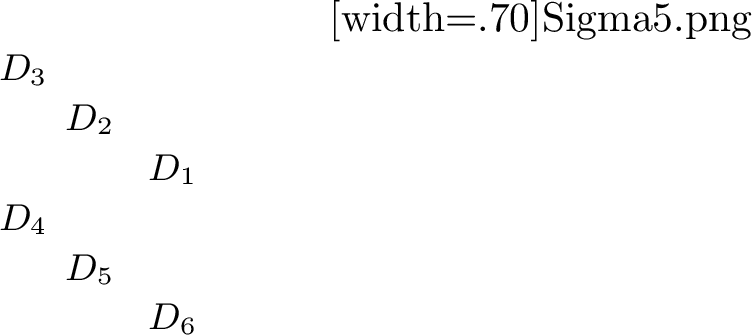
The purpose of this transformation is to eliminate the \((1,3)\) and \((3,1)\) elements of the jump matrix on \({\mathbb{R}}_+\). Let the regions \(\{D_j \}_{j=1}^6\) be as shown in Fig. 5. We define the transformation: \(\mathbf{M}^{(5)}=\mathbf{M}^{(4)} \mathbf{D}(z)\), where the function \(\mathbf{D}(z)\) is given by \[\mathbf{D}(z)=\begin{cases} \mathrm{e}^{\Theta} \begin{pmatrix} 1& 0 & \tilde{r}^*_2(z^*)\\ 0& 1 &0 \\ 0& 0 &1 \end{pmatrix} \mathrm{e}^{-\Theta}, & z \in D_1,\\ \mathrm{e}^{\Theta} \begin{pmatrix} 1& 0 & 0\\ 0& 1 &0 \\ \tilde{r}_2(z)& 0 &1 \end{pmatrix} \mathrm{e}^{-\Theta}, & z \in D_6,\\ \mathrm{e}^{\Theta} \begin{pmatrix} 1& 0 & \tilde{r}^*_2(z^*)+\frac{1}{\gamma(z)}\tilde{r}^*_1(z^*) \tilde{r}_3(z)\\ 0& 1 &0 \\ 0& 0 &1 \end{pmatrix} \mathrm{e}^{-\Theta}, & z \in D_2\cup D_3,\\ \mathrm{e}^{\Theta} \begin{pmatrix} 1& 0 & 0\\ 0& 1 &0 \\ \tilde{r}_2(z)+\frac{1}{\gamma(z)}\tilde{r}_1(z) \tilde{r}^*_3(z^*)& 0 &1 \end{pmatrix} \mathrm{e}^{-\Theta}, & z \in D_4 \cup D_5,\\ \mathbf{I}, & \text{elsewhere}. \end{cases}\] The new jump contour \(\Sigma^{(5)}\) is illustrated in the Fig. 5, and through a direct calculation, one can obtain the expression for the jump matrix \(\mathbf{V}^{(5)}\) as follows: \[\begin{align} &\mathbf{V}^{(5)}_3=\mathrm{e}^{\Theta} \begin{pmatrix} 1& \frac{1}{\gamma(z)} \tilde{r}_1^*(z^*) & 0\\ 0 & 1 & 0\\ 0 & 0 &1 \end{pmatrix} \mathrm{e}^{-\Theta}, \quad \mathbf{V}^{(5)}_6=\mathrm{e}^{\Theta} \begin{pmatrix} 1& 0 & 0\\ -\tilde{r}_1(z) & 1 & 0\\ 0 & 0 &1 \end{pmatrix} \mathrm{e}^{-\Theta},\\ &\mathbf{V}^{(5)}_4=\mathrm{e}^{\Theta}\begin{pmatrix} 1 & 0 & 0\\ 0 & 1 &\tilde{r}_3(z) \\ 0 & 0 &1 \end{pmatrix}\mathrm{e}^{-\Theta}, \quad \mathbf{V}^{(5)}_7=\mathrm{e}^{\Theta}\begin{pmatrix} 1 & 0 & 0\\ 0 & 1 &0 \\ 0 & \frac{1}{\gamma(z)}\tilde{r}^*_3(z^*) &1 \end{pmatrix} \mathrm{e}^{-\Theta},\\ &\mathbf{V}^{(5)}_{9}=\mathrm{e}^{\Theta} \begin{pmatrix} 1& 0 & -\tilde{r}^*_2(z^*)-\frac{1}{\gamma(z)}\tilde{r}^*_1(z^*) \tilde{r}_3(z)\\ 0& 1 &\tilde{r}_3(z) \\ 0& 0 &1 \end{pmatrix} \mathrm{e}^{-\Theta},\\ &\mathbf{V}^{(5)}_{11}=\mathrm{e}^{\Theta} \begin{pmatrix} 1& 0 & 0\\ 0& 1 &0 \\ \tilde{r}_2(z)+\frac{1}{\gamma(z)}\tilde{r}_1(z) \tilde{r}^*_3(z^*)& \frac{1}{\gamma(z)} \tilde{r}^*_3(z^*) &1 \end{pmatrix} \mathrm{e}^{-\Theta}, \\ & \mathbf{V}^{(5)}_{10}=\mathrm{e}^{\Theta} \begin{pmatrix} 1& 0 & 0\\ -\tilde{r}_1(z) & 1 & 0\\ 0 & 0 &1 \end{pmatrix} \begin{pmatrix} 1& \frac{1}{\gamma(z)} \tilde{r}_1^*(z) & 0\\ 0 & 1 & 0\\ 0 & 0 &1 \end{pmatrix} \mathrm{e}^{-\Theta},\\ &\mathbf{V}^{(5)}_{1}=\mathrm{e}^{\Theta}\begin{pmatrix} 1 & 0 & 0\\ 0 & 1 &0 \\ 0 & \frac{1}{\gamma(z)}\tilde{r}^*_3(z) &1 \end{pmatrix} \begin{pmatrix} 1 & 0 & 0\\ 0 & 1 &\tilde{r}_3(z) \\ 0 & 0 &1 \end{pmatrix} \mathrm{e}^{-\Theta}, \qquad \mathbf{V}^{(5)}_5=\mathbf{I}. \end{align}\] The remaining jump matrices either remain unchanged or decay exponentially to the identity matrix \(\mathbf{I}\), and their expressions are omitted for brevity. In addition, the corresponding residue conditions are unaltered.

3.5 The transformations: \(\mathbf{M}^{(5)} \to \mathbf{M}^{(6)} \to \mathbf{M}^{(7)}\)↩︎

The sixth and seventh transformation are intended to extend the remaining jump matrices on \({\mathbb{R}}_+\) appropriately beyond the real axis, ensuring that \(\mathbf{V}^{(7)} - \mathbf{I}\) is uniformly small as \(t \to \infty\). Upon examining the signature tables for \(\mathop{ \mathrm{Re}}\nolimits\phi_{12}(z)\) and \(\mathop{ \mathrm{Re}}\nolimits\phi_{23}(z)\) (see Fig. 1), we find that the lower-upper triangular factorizations of \(\mathbf{V}^{(5)}_1\) and \(\mathbf{V}^{(5)}_{10}\) are no longer suitable. Because such factorizations cannot ensure the extended jump matrix asymptotically approaches the identity matrix. This implies that a new transformation is required to overcome this difficulty.

Let us begin by defining a scalar RH problem: \[\label{E:delta} \begin{cases} \delta_+(z)=\delta_-(z) \left(1+\frac{1}{\gamma(z)}|\tilde{r}_3(z)|^2\right), & z \in \Sigma^{(5)}_{1},\\ \delta(z) \to 1, & z \to \infty. \end{cases}\tag{36}\] Using the symmetry properties of the scattering matrices \(\mathbf{A}(z)\) and \(\mathbf{B}(z)\), a direct computation yields \[0< c< 1+\frac{1}{\gamma(z)}|\tilde{r}_3(z)|^2<C, \;\;\text{for all z \in \Sigma^{(5)}_1 and all \xi \in \mathcal{I}_+.}\] Then the solution to the above RH problem exists and is unique. By the Plemelj’s formula, it can be expressed as \[\label{E:Pbsdel} \delta(z)= \mathrm{exp} \bigg\{ \frac{1}{2 \pi \mathrm{i}} \int_{z_0}^{+\infty} \frac{\ln (1+\frac{1}{\gamma(s)}|\tilde{r}_3(s)|^2)}{s-z} \mathrm{d}s\bigg\}.\tag{37}\] Let \(\tilde{\delta}(z)=\delta(\hat{z})\). Using the relation \[|\rho(z)|=1, \qquad -\frac{1}{\gamma(\hat{z})} |\hat{r}_1(\hat{z})|^2= \frac{1}{\gamma(z)} |\hat{r}_3(z)|^2, \quad \text{for} \;z \in {\mathbb{R}},\] one can find that \(\tilde{\delta}(z)\) satisfies the following RH problem \[\label{E:tildelta} \begin{cases} \tilde{\delta}_+(z)=\tilde{\delta}_-(z) \left(1-\frac{1}{\gamma(z)}|\tilde{r}_1(z)|^2\right)^{-1}, & z \in \Sigma^{(5)}_{10},\\ \tilde{\delta}(z) \to \delta(0), & z \to \infty. \end{cases}\tag{38}\] Thus, \(\tilde{\delta}(z)\) can be expressed as \[\label{E:tildeldel} \tilde{\delta}(z)= \delta(0) \mathrm{exp} \bigg\{ \frac{-1}{2 \pi \mathrm{i}} \int_{0}^{z_1} \frac{\ln (1-\frac{1}{\gamma(s)}|\tilde{r}_1(s)|^2)}{s-z} \mathrm{d}s\bigg\}.\tag{39}\] Let \(\log_{\theta}(z)\) denote the logarithm of \(z\) with branch cut along \(\mathrm{arg} z=\theta\), i.e., \[\log_0(z)=\ln|z|+\mathrm{arg}_0(z), \quad \mathrm{arg}_0(z)\in(0,2\pi);\quad \log_{\pi}(z)=\ln|z|+\mathrm{arg}_{\pi}(z),\quad \mathrm{arg}_{\pi}(z)\in(-\pi,\pi).\] Then the following lemma collect the basic properties of the functions \(\delta(z)\) and \(\tilde{\delta}(z)\).

We partition the set \(\{0,1,..,N-1 \}\) into the pair of sets \[\nabla^+=\big\{j:\mathop{ \mathrm{Re}}\nolimits\zeta_j > \xi \big\},\qquad \nabla^-=\big\{j: \mathop{ \mathrm{Re}}\nolimits\zeta_j \leq \xi \big\}.\] We define \(\mathcal{P}_1(z)=\prod_{j \in \nabla^+}\frac{z-\zeta_j}{z-\zeta_j^*}\) and introduce the following two diagonal matrices: \[\label{E:DelP} \tilde{\mathbf{\Delta}}(z)=\begin{pmatrix} 1/\tilde{\delta}(z)& & \\ & \delta(z) \tilde{\delta}(z)& \\ & &1/\delta(z) \end{pmatrix}, \qquad \mathbf{P}(z)= \begin{pmatrix} \mathcal{P}_1(z)& & \\ & 1/\left(\mathcal{P}_1(z)\mathcal{P}_1(\hat{z}) \right )& \\ & &\mathcal{P}_1(\hat{z}) \end{pmatrix}.\tag{40}\] Then, let \(\mathbf{T}(z)=\tilde{\mathbf{\Delta}}(z) \mathbf{P}(z):= \mathrm{diag}\left(T_1(z), T_2(z), T_3(z) \right)\). It is easy to see that \(T_1(z)=\delta(z) \mathcal{P}_1(z)\), \(T_3(z)=T_1(\hat{z})\), \(T_2(z)=1/(T_1(z)T_3(z))\). Then, through a direct calculation, one can verify that \(\mathbf{\Pi}^{-1}(z) \mathbf{T}(\hat{z}) \mathbf{\Pi}(z)=\mathbf{T}(z)\). Moreover, it should be noted that \(\mathbf{T}(z)\) does not approach the identity matrix as \(z \to \infty\). In fact, we have \[\mathbf{T}(z)\to \mathbf{T}^{\infty}, \;\;z \to \infty,\;\; \text{where} \;\;\mathbf{T}^{\infty}= \tilde{\mathbf{\Delta}}^{\infty} \mathbf{P}^{\infty},\] with \[\label{E:DPinfty} \tilde{\mathbf{\Delta}}^{\infty}=\mathrm{diag}\left(1/\delta(0), \delta(0),1 \right), \quad \mathbf{P}^{\infty}=\mathrm{diag} \left(1, \displaystyle \prod_{j \in \nabla^+} \frac{q_0^2}{\zeta_j^2} , \displaystyle \prod_{j \in \nabla^+} \frac{\zeta_j^2}{q_0^2} \right).\tag{41}\]

We define the sixth transformation as follows: \[\mathbf{M}^{(6)}(x,t,z)=(\tilde{\mathbf{\Delta}}^{\infty})^{-1}\mathbf{M}^{(5)}(x,t,z)\mathbf{T}(z), \qquad z \in \mathbb{C}.\] The jump contour remains unchanged. The new jump matrix can be calculated using the formula \(\mathbf{V}^{(6)}=\mathbf{T}_-^{-1} \mathbf{V}^{(5)} \mathbf{T}_+\). Specifically, we provide the jumps along several of these contours below. \[\begin{align} &\mathbf{V}^{(6)}_{10}=\mathrm{e}^{\Theta} \begin{pmatrix} 1& \frac{1}{\gamma(z)}\frac{\tilde{r}_1^*(z)}{1-\frac{1}{\gamma(z)} |\tilde{r}_1(z)|^2 } \frac{T_{2,-}}{T_{1,-}}(z)& 0\\ 0 & 1 & 0\\ 0 & 0 &1 \end{pmatrix} \begin{pmatrix} 1& 0 & 0\\ -\frac{\tilde{r}_1(z)}{1-\frac{1}{\gamma(z)} |\tilde{r}_1(z)|^2} \frac{T_{1,+}}{T_{2,+}}(z) & 1 & 0\\ 0 & 0 &1 \end{pmatrix} \mathrm{e}^{-\Theta},\\ &\mathbf{V}^{(6)}_3=\mathrm{e}^{\Theta} \begin{pmatrix} 1& \frac{1}{\gamma(z)} \tilde{r}_1^*(z^*)\frac{T_2}{T_1}(z) & 0\\ 0 & 1 & 0\\ 0 & 0 &1 \end{pmatrix} \mathrm{e}^{-\Theta}, \quad \mathbf{V}^{(6)}_6=\mathrm{e}^{\Theta} \begin{pmatrix} 1& 0 & 0\\ -\tilde{r}_1(z)\frac{T_1}{T_2}(z) & 1 & 0\\ 0 & 0 &1 \end{pmatrix} \mathrm{e}^{-\Theta},\\ &\mathbf{V}^{(6)}_4=\mathrm{e}^{\Theta}\begin{pmatrix} 1 & 0 & 0\\ 0 & 1 &\tilde{r}_3(z)\frac{T_3}{T_2}(z) \\ 0 & 0 &1 \end{pmatrix}\mathrm{e}^{-\Theta}, \quad \mathbf{V}^{(6)}_7=\mathrm{e}^{\Theta}\begin{pmatrix} 1 & 0 & 0\\ 0 & 1 &0 \\ 0 & \frac{1}{\gamma(z)}\tilde{r}^*_3(z^*)\frac{T_2}{T_3}(z) &1 \end{pmatrix} \mathrm{e}^{-\Theta}\\ &\mathbf{V}^{(6)}_{1}=\mathrm{e}^{\Theta}\begin{pmatrix} 1 & 0 & 0\\ 0 & 1 &\frac{\tilde{r}_3(z)}{1+\frac{1}{\gamma(z)} |\tilde{r}_3(z) |^2} \frac{T_{3,-}}{T_{2,-}}(z) \\ 0 & 0 &1 \end{pmatrix} \begin{pmatrix} 1 & 0 & 0\\ 0 & 1 & 0\\ 0 & \frac{1}{\gamma(z)}\frac{\tilde{r}^*_3(z)}{1+\frac{1}{\gamma(z)} |\tilde{r}_3(z)|^2} \frac{T_{2,+}}{T_{3,+}}(z) &1 \end{pmatrix} \mathrm{e}^{-\Theta}. \end{align}\] One will see that on the remaining jump contours, \(\mathbf{V}^{(6)}-\mathbf{I}\) is uniformly small as \(t \to \infty\); thus, we omit their expressions for brevity. Note that this transformation will alter the residue conditions, so we need to clarify the current residue conditions.

We now examine the behavior of \(\mathbf{M}^{(6)}\) near the branch points \(\pm q_0\). It is readily observed that \(\mathbf{M}^{(6)}\) exhibits no jump in the neighborhood of \(\pm q_0\), and the values of \(\mathbf{M}^{(6)}\) at \(\pm q_0\) exist. Furthermore, we have the following lemma:

Now, \(\mathbf{V}^{(6)}_1\) and \(\mathbf{V}_{10}^{(6)}\) are already in the desired upper-lower triangular factorization form. Our next transformation is aimed at analytically extending them beyond the real axis. Define \(\mathbf{M}^{(7)}(x,t,z)=\mathbf{M}^{(6)}(x,t,z) \mathbf{N}(x,t,z)\), where \(\mathbf{N}(x,t,z)\) is given by \[\label{E:exN} \mathbf{N}(x,t,z)= \begin{cases} \mathrm{e}^{\Theta} \begin{pmatrix} 1& 0 & 0\\ \frac{\tilde{r}_1(z)}{1-\frac{1}{\gamma(z)} \tilde{r}_1(z) \tilde{r}^*_1(z^*) } \frac{T_{1}}{T_{2}}(z) & 1 & 0\\ 0 & 0 &1 \end{pmatrix} \mathrm{e}^{-\Theta}, & z \in U_3 \cup U_5,\\ \mathrm{e}^{\Theta} \begin{pmatrix} 1& \frac{1}{\gamma(z)}\frac{\tilde{r}_1^*(z^*)}{1-\frac{1}{\gamma(z)} \tilde{r}_1(z) \tilde{r}^*_1(z^*)} \frac{T_{2}}{T_{1}}(z)& 0\\ 0 & 1 & 0\\ 0 & 0 &1 \end{pmatrix}\mathrm{e}^{-\Theta}, & z \in U_4,\\ \mathrm{e}^{\Theta} \begin{pmatrix} 1& 0& 0\\ 0 & 1 & 0\\ 0 & - \frac{1}{\gamma(z)} \frac{\tilde{r}_3^*(z^*)}{1+\frac{1}{\gamma(z)} \tilde{r}_3(z) \tilde{r}^*_3(z^*)} \frac{T_{2}}{T_{3}}(z) &1 \end{pmatrix}\mathrm{e}^{-\Theta}, & z \in U_1,\\ \mathrm{e}^{\Theta} \begin{pmatrix} 1& 0 & 0\\ 0& 1 &\frac{\tilde{r}_3(z)}{1+\frac{1}{\gamma(z)} \tilde{r}_3(z) \tilde{r}^*_3(z^*)} \frac{T_{3}}{T_{2}}(z) \\ 0 & 0 &1 \end{pmatrix} \mathrm{e}^{-\Theta}, & z \in U_2. \end{cases}\tag{43}\] Here, the regions \(\{ U_j\}_{j=1}^5\) are as shown in Fig. 6. The new jump matrix \(\mathbf{V}^{(7)}\) can be written as \(\mathbf{V}^{(7)}=\mathbf{N}_-^{-1} \mathbf{V}^{(6)} \mathbf{N}_+\). It follows by direct computation that \[\begin{align} &\mathbf{V}^{(7)}_6= \mathrm{e}^{\Theta} \begin{pmatrix} 1& 0 & 0\\ -\frac{\tilde{r}_1(z)}{1-\frac{1}{\gamma(z)} \tilde{r}_1(z) \tilde{r}^*_1(z^*) } \frac{T_{1}}{T_{2}}(z) & 1 & 0\\ 0 & 0 &1 \end{pmatrix} \mathrm{e}^{-\Theta}, \;\; \mathbf{V}^{(7)}_5=\mathrm{e}^{\Theta} \begin{pmatrix} 1& \frac{1}{\gamma(z)} \tilde{r}_1^*(z^*) \frac{T_2}{T_1}(z) & 0\\ 0& 1 &0 \\ 0&0 &1 \end{pmatrix} \mathrm{e}^{-\Theta},\\ &\mathbf{V}^{(7)}_8=\mathrm{e}^{\Theta} \begin{pmatrix} 1& 0 & 0\\ -\tilde{r}_1(z) \frac{T_1}{T_2}(z)& 1 &0 \\ 0&0 &1 \end{pmatrix} \mathrm{e}^{-\Theta}, \;\; \mathbf{V}^{(7)}_7= \mathrm{e}^{\Theta} \begin{pmatrix} 1& \frac{1}{\gamma(z)}\frac{\tilde{r}^*_1(z^*)}{1-\frac{1}{\gamma(z)} \tilde{r}_1(z) \tilde{r}^*_1(z^*) } \frac{T_{1}}{T_{2}}(z)& 0\\ 0 & 1 & 0\\ 0 & 0 &1 \end{pmatrix} \mathrm{e}^{-\Theta},\\ &\mathbf{V}^{(7)}_2=\mathrm{e}^{\Theta}\begin{pmatrix} 1 & 0 & 0\\ 0 & 1 &\tilde{r}_3(z)\frac{T_3}{T_2}(z) \\ 0 & 0 &1 \end{pmatrix}\mathrm{e}^{-\Theta},\;\; \mathbf{V}^{(7)}_3=\mathrm{e}^{\Theta}\begin{pmatrix} 1 & 0 & 0\\ 0 & 1 &0 \\ 0 & \frac{1}{\gamma(z)}\tilde{r}^*_3(z^*)\frac{T_2}{T_3}(z) &1 \end{pmatrix} \mathrm{e}^{-\Theta},\\ &\mathbf{V}^{(7)}_1=\mathrm{e}^{\Theta} \begin{pmatrix} 1& 0& 0\\ 0 & 1 &0 \\ 0& \frac{1}{\gamma(z)} \frac{\tilde{r}_3^*(z^*)}{1+\frac{1}{\gamma(z)} \tilde{r}_3(z) \tilde{r}^*_3(z^*)} \frac{T_{2}}{T_{3}}(z) &1 \end{pmatrix} \mathrm{e}^{-\Theta}, \; \mathbf{V}^{(7)}_{4}=\mathrm{e}^{\Theta} \begin{pmatrix} 1& 0 & 0\\ 0 & 1 & \frac{\tilde{r}_3(z)}{1+\frac{1}{\gamma(z)} \tilde{r}_3(z) \tilde{r}^*_3(z^*)} \frac{T_{3}}{T_{2}}(z) \\ 0& 0 &1 \end{pmatrix} \mathrm{e}^{-\Theta},\\ &\mathbf{V}^{(7)}_{10}=\mathrm{e}^{\Theta} \begin{pmatrix} 1&0&0\\ \left( r_1(z) \delta^2_1(z) \delta_1(\hat{z})+\frac{\tilde{r}_1(z)}{1-\frac{1}{\gamma(z)} \tilde{r}_1(z) \tilde{r}^*_1(z^*) } \right) \frac{T_1}{T_2}(z)&1&0\\ \left( r_2(z) \frac{\delta_1(z)}{\delta_1(\hat{z})} - \frac{1}{\gamma(z) \delta_1(z) \delta_1^2(\hat{z})} \frac{\tilde{r}_1(z) \tilde{r}^*_3(z^*) }{1-\frac{1}{\gamma(z)} \tilde{r}_1(z) \tilde{r}^*_1(z^*) }\right) \frac{T_3}{T_1}(z)&-\frac{1}{\gamma(z)}r_3^* (z^*)\frac{1}{\delta_1(z) \delta_1^2(\hat{z})} \frac{T_2}{T_3}(z)&1 \end{pmatrix} \mathrm{e}^{-\Theta}.\\ \end{align}\] For simplicity, we omit the exact expressions for the remaining jumps. On the other hand, one can verify that \(\mathbf{M}^{(7)}\) and \(\mathbf{M}^{(6)}\) satisfy the same residue conditions, and the details will not be repeated here.

Let \(D_{\epsilon}(z_0)\) and \(D_{\epsilon}(z_1)\) denote two small disks around \(z_0\) and \(z_1\), respectively. Define \(\mathcal{D}=D_{\epsilon}(z_0) \cup D_{\epsilon}(z_1)\), then we prove that outside \(\mathcal{D}\), \(\mathbf{V}^{(7)} - \mathbf{I}\) is uniformly small as \(t \to \infty\).

3.6 The outer parametrix and the local parametrix↩︎

In this subsection, we first seek a RH problem that has no jump but satisfies the same residue conditions and asymptotic properties as \(\mathbf{M}^{(7)}(x,t,z)\). We refer to the solution of such a RH problem as the outer parametrix. We will now demonstrate how to explicitly construct it.

We begin by considering the following modulated pure-soliton RH problem.

We define the function \(\mathbf{M}^{out}\) as \[\label{E:Mout} \mathbf{M}^{out}(x,t,z)=(\mathbf{M}_{\infty})^{-1}\mathbf{M}_{msol}(x,t,z) \mathbf{P}(z),\tag{46}\] where \(\mathbf{P}(z)\) is given by 40 . The function \(\mathbf{M}^{out}\) serves as the outer parametrix we require, and it satisfies the same residue conditions and asymptotic properties as \(\mathbf{M}^{(7)}\). Let \(D_{sig}\) denote a small neighborhood which contains the origin and the discrete spectrum set. Then it can be verified that \(\mathbf{M}^{out}\) and \((\mathbf{M}^{out})^{-1}\) are uniformly bounded for \(z \in \mathbb{C}\setminus D_{sig}\) and \(\xi \in \mathcal{I}_+\).

Next, we proceed to construct the local models. In the previous subections, we have shown that the jump matrix \(\mathbf{V}^{(7)}\) decays uniformly to \(\mathbf{I}\) except in the vicinity of the two critical points \(z_0\) and \(z_1\). We will show that \(\mathbf{M}^{(7)}\) can be approximated locally near the two critical points by solutions of solvable model RH problems. Let \(D_{\epsilon }(z_0)\) and \(D_{\epsilon }(z_1)\) denote small disks of radius \(\epsilon\) with centers at \(z_0\) and \(z_1\) respectively. Define \(\mathcal{D}=D_{\epsilon }(z_0) \cup D_{\epsilon }(z_1)\). Let \[X^L:=z_1+X, \qquad X^R:=z_0+X,\qquad X^L_j:=z_1+X_j, \qquad X^R_j:=z_0+X_j,\] where \(X=\cup_{j=1}^4 X_j\) and \(X_j\) is defined in 121 . We also define \[\begin{align} X^{L,\epsilon}=X^L \cap D_{\epsilon }(z_1), \quad X^{R,\epsilon}=X^R \cap D_{\epsilon }(z_0), \quad X^{L,\epsilon}_j=X^L_j \cap D_{\epsilon }(z_1), \quad X^{R,\epsilon}_j=X^R_j \cap D_{\epsilon }(z_0). \end{align}\] We then introduce two new variables in the neighborhoods of \(z_1\) and \(z_0\) respectively: \[\begin{align} \label{E:yellr} y_{\ell}=\sqrt{2t}(z-z_1), \qquad z \in D_{\epsilon }(z_1);\qquad y_{r}=\frac{\xi^2}{q_0^2}\sqrt{2t}(z-z_0), \qquad z \in D_{\epsilon }(z_0). \end{align}\tag{47}\] By performing Taylor expansions of the functions \(\theta_{32}(x,t,z)\) and \(\theta_{21}(x,t,z)\) at \(z_1\) and \(z_0\) respectively, we obtain \[\begin{align} \label{E:thetabs} \theta_{21}(x,t,z)-\theta_{21}(x,t,z_1)=-\frac{\mathrm{i}}{2}y_{\ell}^2,\qquad \theta_{32}(x,t,z)-\theta_{32}(x,t,z_0)=\frac{\mathrm{i}}{2}y_{r}^2+\theta_r(x,t,z), \end{align}\tag{48}\] where \[\theta_{r}(x,t,z)=\mathcal{O}(z-z_0)^3, \;\; \text{as z \to z_0.}\] From Eq. 30 , we have \[\label{E:zhsh} \begin{align} \tilde{r}_1(z)\frac{T_{1}}{T_{2}}(z) =& \hat{r}_1(z) \rho^2(z) \rho(\hat{z}) \frac{\mathcal{P}^2_1(z) \mathcal{P}_1(\hat{z})}{\delta(z) \delta^2(\hat{z})},\\ \tilde{r}^*_3(z^*)\frac{T_{2}}{T_{3}}(z)=&\hat{r}^*_3(z^*) \frac{\delta^2(z) \delta(\hat{z})}{\rho(z)\rho^2(\hat{z}) \mathcal{P}_1(z) \mathcal{P}_1^2(\hat{z})}. \end{align}\tag{49}\] Eqs. ?? and 47 imply that, for \(\xi \in \mathcal{I}_+\) \[\label{E:T12} \begin{align} &\frac{\delta^2(z) \delta(\hat{z})}{\rho(z)\rho^2(\hat{z}) \mathcal{P}_1(z) \mathcal{P}_1^2(\hat{z})}=\mathrm{e}^{-2 \mathrm{i}\nu \log_{0} y_r} d_0^r d_1^r, \qquad z \in D_{\epsilon}(z_0) \setminus [z_0,\infty),\\ & \rho^2(z) \rho(\hat{z}) \frac{\mathcal{P}^2_1(z) \mathcal{P}_1(\hat{z})}{\delta(z) \delta^2(\hat{z})}= \mathrm{e}^{2 \mathrm{i}\tilde{\nu} \log_{\pi} y_{\ell}}d_0^{\ell} d_1^{\ell}, \qquad z \in D_{\epsilon}(z_1) \setminus [0,z_1], \end{align}\tag{50}\] where \[\begin{align} &d_0^r=(\frac{q_0^2}{\xi^2 \sqrt{2t}})^{-2 \mathrm{i}\nu} \mathrm{e}^{-2 \chi(z_0)} \frac{\delta(z_1)}{ \rho^2(z_1)\rho(z_0) \mathcal{P}_1(z_0) \mathcal{P}_1^2(z_1)}, \tag{51}\\ &d_1^r=\frac{\delta(\hat{z}) \rho^2(z_1)\rho(z_0) \mathcal{P}_1^2(z_1) \mathcal{P}_1(z_0)}{\delta(z_1) \rho(z) \rho^2(\hat{z}) \mathcal{P}_1(z) \mathcal{P}^2_1(\hat{z})} \mathrm{e}^{-2 \chi(z)+2\chi(z_0)},\\ &d_0^{\ell}=(\sqrt{2t})^{-2 \mathrm{i}\tilde{\nu}} \frac{\rho^2(z_1) \rho(z_0) \mathcal{P}^2_1(z_1) \mathcal{P}_1(z_0) }{\delta^2(0)\delta(z_1) } \mathrm{e}^{-2 \tilde{\chi} (z_1)},\tag{52}\\ &d_1^{\ell}=\frac{\delta(z_1) \rho(\hat{z}) \rho^2(z) \mathcal{P}_1(\hat{z}) \mathcal{P}_1^2(z)}{\delta(z) \rho^2(z_1)\rho(z_0) \mathcal{P}_1^2(z_1) \mathcal{P}_1(z_0)} \mathrm{e}^{-2 \tilde{\chi}(z)+2\tilde{\chi}(z_1)}. \end{align}\] In order to relate \(\mathbf{M}^{(7)}\) to the solutions of model RH problems, we define \[\label{E:Y} \mathbf{Y}(\xi,t)=\begin{cases} \mathbf{Y}_L(\xi,t), &z \in D_{\epsilon}(z_1),\\ \mathbf{Y}_R(\xi,t), & z \in D_{\epsilon}(z_0), \end{cases}\tag{53}\] where \[\label{E:YLYR} \begin{align} &\mathbf{Y}_R(\xi,t)=\begin{pmatrix} 1& &\\ & (d_0^{r})^{-1/2}\mathrm{e}^{-\frac{\theta_{32}(x,t,z_0)}{2}}&\\ & & (d_0^{r})^{1/2}\mathrm{e}^{\frac{\theta_{32}(x,t,z_0)}{2}} \end{pmatrix}, \\ &\mathbf{Y}_L(\xi,t)=\begin{pmatrix} (d_0^{\ell})^{-1/2}\mathrm{e}^{-\frac{\theta_{21}(x,t,z_1)}{2}}& &\\ &(d_0^{\ell})^{1/2}\mathrm{e}^{\frac{\theta_{21}(x,t,z_1)}{2}} &\\ & & 1 \end{pmatrix}. \end{align}\tag{54}\]

Define \(\tilde{\mathbf{M}}\) for \(z\) near \(z_0\) and \(z_1\) by \[\tilde{\mathbf{M}}(x,t,z)=\mathbf{M}^{(7)}(x,t,z) \mathbf{Y}(\xi,z), \qquad z \in \mathcal{D}.\] Clearly, the jump matrix \(\tilde{\mathbf{V}}=\mathbf{Y}^{-1} \mathbf{V}^{(7)} \mathbf{Y}\). Let \(\tilde{\mathbf{V}}|_{X^{R,\epsilon}_j}\) denotes the restriction of \(\tilde{\mathbf{V}}\) to \(X^{R,\epsilon}_j\), \(j=1,2,3,4\). For a fixed \(y_r\), \(\hat{r}_3(z) \to \hat{r}_3(z_0)\) and \(d_{1}^r(z) \to 1\) as \(t \to \infty\). This suggests that \(\tilde{\mathbf{V}}|_{X^{R,\epsilon}_j}\) tends to the jump matrix \(\mathbf{V}^{X,R}_j(x,t,y_r)\) defined in Appendix 9.1 for large \(t\). Through a similar discussion, one can easily find that \(\tilde{\mathbf{V}}|_{X^{L,\epsilon}_j} \to \mathbf{V}^{X,L}_j(x,t,y_{\ell})\) as \(t \to \infty\). The above analysis suggests that we can approximate \(\mathbf{M}^{(7)}(x,t,z)\) in \(\mathcal{D}\) by the \(3 \times 3\)-matrix-valued function \(\mathbf{M}^{loc}(x,t,z)\) defined by \[\label{E:Mloc} \mathbf{M}^{loc}(x,t,z)=\begin{cases} \mathbf{Y}_L(\xi,t) \mathbf{M}^{X,L}(x,t,z) \mathbf{Y}_L^{-1}(\xi,z), & z \in D_{\epsilon}(z_1),\\ \mathbf{Y}_R(\xi,t) \mathbf{M}^{X,R}(x,t,z) \mathbf{Y}_R^{-1}(\xi,z), & z \in D_{\epsilon}(z_0). \end{cases}\tag{55}\] Here, \(\mathbf{M}^{X,L}(x,t,z)\) and \(\mathbf{M}^{X,R}(x,t,z)\) are the solutions to the model RH problems defined in Appendix 9.1. The prefactors \(\mathbf{Y}_L(\zeta,t)\) and \(\mathbf{Y}_R(\zeta,t)\) on the right-hand side of 55 are included so that \(\mathbf{M}^{loc} \to \mathbf{I}\) on \(\partial \mathcal{D}\) as \(t \to \infty\); this ensures that \(\mathbf{M}^{loc}\) is a good approximation of \(\mathbf{M}^{(7)}\) in \(\mathcal{D}\) for large \(t\).

Let \(X^{\epsilon}\) be defined as \(X^{\epsilon}=X^{R,\epsilon} \cup X^{L,\epsilon}\), and let the boundary \(\partial \mathcal{D}\) of \(\mathcal{D}\) be oriented counterclockwise. Then we have the following lemma.

3.7 Final Transformation: \(\mathbf{M}^{(7)} \to \boldsymbol{\mathcal{E}}\)↩︎

We define the final transformation to obtain a small-norm RH problem as follows: \[\label{E:defE} \boldsymbol{\mathcal{E}}(x,t,z)=\begin{cases} \mathbf{M}^{(7)}(x,t,z)(\mathbf{M}^{out})^{-1}(x,t,z), & z\in \mathbb{C}\setminus \mathcal{D},\\ \mathbf{M}^{(7)}(x,t,z)(\mathbf{M}^{loc})^{-1}(x,t,z)(\mathbf{M}^{out})^{-1}(x,t,z), &z \in \mathcal{D}. \end{cases}\tag{56}\] We will show that \(\boldsymbol{\mathcal{E}}(x,t,z)\) is close to \(\mathbf{I}\) for large \(t\) and \(\xi \in \mathcal{I}_{+}\). We first note that although \(\mathbf{M}^{(7)}(x,t,z)\) has a singularity at \(0\) and \((\mathbf{M}^{out})^{-1}(x,t,z)\) has singularities at the branch points \(\pm q_0\), the function \(\boldsymbol{\mathcal{E}}(x,,t,z)\) is well-defined at these points.

Let \(\Sigma^{\mathcal{E}}=\Sigma^{(7)} \cup \partial \mathcal{D}\), and define the matrix-valued function \(\mathbf{V}^{\mathcal{E}}(x,t,z)\) for \(z \in \Sigma^{\mathcal{E}}\) as follows: \[\label{E:VEex} \mathbf{V}^{\mathcal{E}}(x,t,z)=\begin{cases} \mathbf{M}^{out} \mathbf{V}^{(7)}(\mathbf{M}^{out})^{-1}, & z \in \Sigma^{\mathcal{E}} \setminus \bar{\mathcal{D}},\\ \mathbf{M}^{out}(\mathbf{M}^{loc})^{-1}(\mathbf{M}^{out})^{-1}, & z\in \partial \mathcal{D},\\ \mathbf{M}^{out}\left( \mathbf{M}^{loc}_- \mathbf{V}^{(7)} (\mathbf{M}^{loc}_+)^{-1} \right)(\mathbf{M}^{out})^{-1}, & z \in X^{\epsilon}. \end{cases}\tag{61}\] A direct verification shows that \(\boldsymbol{\mathcal{E}}(x,t,z)\) satisfies the following RH problem:

The estimates in Lemma 16 show that \[\begin{align} \begin{cases} \|\mathbf{w}^{\mathcal{E}} \|_{L^1 (\Sigma^{\mathcal{E}})} \leq C t^{-1}\ln t\\ \|\mathbf{w}^{\mathcal{E}} \|_{L^{\infty} (\Sigma^{\mathcal{E}})} \leq C t^{-1/2}\ln t \end{cases} \qquad \xi \in \mathcal{I}_+, \;\;t>2. \end{align}\] Thus by employing the general inequality \(\|f \|_{L^p} \leq \| f\|_{L^1}^{\frac{1}{p}} \|f \|_{L^{\infty}}^{\frac{p-1}{p}}\), we immediately get \[\begin{align} \label{E:wELp} \|\mathbf{w}^{\mathcal{E}} \|_{L^p (\Sigma^{\mathcal{E}})} \leq C t^{-1/2}(\ln t)^{(p-1)/p}, \qquad \xi \in \mathcal{I}_+, \;\;t>2. \end{align}\tag{62}\] For the contour \(\Sigma^{\mathcal{E}}\) and a function \(\mathbf{h}(z) \in L^2(\Sigma^{\mathcal{E}})\), we define the Cauchy transform \(\mathcal{C}(\mathbf{h})(z)\) associated with \(\Sigma^{\mathcal{E}}\) by \[\mathcal{C}(\mathbf{h})(z) := \frac{1}{2\pi \mathrm{i}}\int_{\Sigma^{\mathcal{E}}}\frac{\mathbf{h}(z')dz'}{z'-z}.\] It is kown that the left and right non-tangential boundary values \(\mathcal{C}_+\mathbf{h}\) and \(\mathcal{C}_-\mathbf{h}\) of \(\mathcal{C}(\mathbf{h})\) exist a.e. on \(\Sigma^{\mathcal{E}}\) and belong to \(L^2(\Sigma^{\mathcal{E}})\). Let \(\mathcal{B}(L^2(\Sigma^{\mathcal{E}}))\) denotes the space of bounded linear operators on \(L^2(\Sigma^{\mathcal{E}})\). Then \(\mathcal{C}_{\pm} \in \mathcal{B}(L^2(\Sigma^{\mathcal{E}}))\) and \(\mathcal{C}_+-\mathcal{C}_-=I\), where \(I\) denotes the identity operator on \(L^2(\Sigma^{\mathcal{E}})\). Furthermore, we define the operator \(\mathcal{C}_{\mathbf{w}^{\mathcal{E}}}\) by \(\mathcal{C}_{\mathbf{w}^{\mathcal{E}}}(\mathbf{h})=\mathcal{C}_-(\mathbf{h}\mathbf{w}^{\mathcal{E}})\). From the preceding analysis, we have known that \(\|\mathbf{w}^{\mathcal{E}}\|_{L^2(\Sigma^{\mathcal{E}})} \to 0\) as \(t \to \infty\). Consequently, there exists a \(T>0\) such that the operator \(I-\mathcal{C}_{\mathbf{w}^{\mathcal{E}}}\) is invertible whenever \(t>T\) and \(\xi \in \mathcal{I}_+\). Therefore, we can define a function \(\mathbf{u}^{\mathcal{E}}(x,t,z)\) for \(z \in \Sigma^{\mathcal{E}}\) and \(t>T\) by \[\begin{align} \label{E:uE} \mathbf{u}^{\mathcal{E}}=\mathbf{I}+(I-\mathcal{C}_{\mathbf{w}^{\mathcal{E}}})^{-1}\mathcal{C}_{\mathbf{w}^{\mathcal{E}}}\mathbf{I}\;\in \mathbf{I}+ L^2(\Sigma^{\mathcal{E}}). \end{align}\tag{63}\] We need the estimate of \(\|\mathbf{u}^{\mathcal{E}} -\mathbf{I}\|_{L^2(\Sigma^{\mathcal{E}})}\) when \(t\) is sufficiently large. From 62 and 63 , it follows that \[\label{E:yxjs11} \begin{align} \|\mathbf{u}^{\mathcal{E}} - \mathbf{I}\|_{L^2(\Sigma^{\mathcal{E}})}&\leq \|(I-\mathcal{C}_{\mathbf{w}^{\mathcal{E}}})^{-1}\mathcal{C}_{\mathbf{w}^{\mathcal{E}}}\mathbf{I}\|_{L^2(\Sigma^{\mathcal{E}})}\\ &\leq \sum_{j=1}^{\infty}\| \mathcal{C}_{\mathbf{w}^{\mathcal{E}}}\|_{\mathcal{B}(L^2(\Sigma^{\mathcal{E}}))}\|\mathcal{C}_{\mathbf{w}^{\mathcal{E}}} \mathbf{I}\|_{L^2(\Sigma^{\mathcal{E}})}\\ &\leq \frac{\|\mathcal{C}_- \|_{\mathcal{B}(L^2(\Sigma^{\mathcal{E}}))} \| \mathbf{w}^{\mathcal{E}}\|_{L^2(\Sigma^{\mathcal{E}})}}{1-\|\mathcal{C}_- \|_{\mathcal{B}(L^2(\Sigma^{\mathcal{E}}))} \|\mathbf{w}^{\mathcal{E}} \|_{L^{\infty}(\Sigma^{\mathcal{E}})}}\\ & \leq Ct^{-1/2}(\ln t)^{1/2}, \qquad t>T. \end{align}\tag{64}\] According to the standard theory of RH problems [25], [45], [55], \(\boldsymbol{\mathcal{E}}(x,t,z)\) can be expressed as \[\label{E:Ejfbs} \boldsymbol{\mathcal{E}}(x,t,z)=\mathbf{I}+\frac{1}{2\pi \mathrm{i}}\int_{\Sigma^{\mathcal{E}}}\frac{\mathbf{u}^{\mathcal{E}}(z') \mathbf{w}^{\mathcal{E}} (z')dz'}{z'-z}, \qquad z \in \mathbb{C}\setminus \Sigma^{\mathcal{E}}.\tag{65}\] From 65 , we know the following nontangential limit is well-defined: \[\begin{align} \label{E:L} \mathbf{L}(x,t):=\lim^{\angle}_{z \to \infty}(\boldsymbol{\mathcal{E}}(x,t,z)-\mathbf{I})=-\frac{1}{2\pi \mathrm{i}}\int_{\Sigma^{\mathcal{E}}}\mathbf{u}^{\mathcal{E}} (x,t,\zeta)\mathbf{w}^{\mathcal{E}}(x,t,\zeta) \mathrm{d}\zeta. \end{align}\tag{66}\]

Recall that when \(z \in \partial \mathcal{D}\), we have \[\mathbf{w}^{\mathcal{E}}(x,t,z)=\mathbf{M}^{out}(x,t,z)(\mathbf{M}^{loc})^{-1}(x,t,z)(\mathbf{M}^{out})^{-1}(x,t,z)-\mathbf{I},\] thus we obtain \[\label{E:wEyy} \begin{align} \mathbf{w}^{\mathcal{E}}(x,t,z)=-\frac{\mathbf{M}^{out}(x,t,z) \mathbf{Y}_R(\xi,t) \mathbf{M}^{X,R}_{\infty} \mathbf{Y}^{-1}_R(\xi,t) (\mathbf{M}^{out})^{-1}(x,t,z) }{\frac{\xi^2}{q_0^2} \sqrt{2t} (z-z_0)}+\mathcal{O}(t^{-1})&, \\ z \in \partial D_{\epsilon}(z_0), \quad t \to \infty ,\\ \mathbf{w}^{\mathcal{E}}(x,t,z)=-\frac{\mathbf{M}^{out}(x,t,z) \mathbf{Y}_L(\xi,t) \mathbf{M}^{X,L}_{\infty} \mathbf{Y}^{-1}_L(\xi,t) (\mathbf{M}^{out})^{-1}(x,t,z) }{ \sqrt{2t} (z-z_1)}+\mathcal{O}(t^{-1})&, \\ z \in \partial D_{\epsilon}(z_1), \quad t \to \infty . \end{align}\tag{67}\] We define the functions \(F^{(1)}(\xi,t)\) and \(F^{(2)}(\xi,t)\) by \[\label{E:F12} F^{(1)}(\xi,t)=-\frac{1}{2\pi \mathrm{i}} \int_{\partial D_{\epsilon}(z_0)} \mathbf{w}^{\mathcal{E}}(x,t,\zeta) \mathrm{d} \zeta, \quad F^{(2)}(\xi,t)=-\frac{1}{2\pi \mathrm{i}} \int_{\partial D_{\epsilon}(z_1)} \mathbf{w}^{\mathcal{E}}(x,t,\zeta) \mathrm{d} \zeta.\tag{68}\] Recalling the definitions of \(\mathbf{M}^{out}\), \(\mathbf{Y}_L\), \(\mathbf{Y}_R\), \(\mathbf{M}^{X,L}_{\infty}\) and \(\mathbf{M}^{X,R}_{\infty}\), using Eq. 67 and applying the residue theorem, we obtain \[\begin{align} F^{(1)}(\xi,t)&=\frac{q_0^2}{\xi^2 \sqrt{2t}} \mathbf{M}^{out}(x,t,z_0) \mathbf{Y}_R(\xi,t) \mathbf{M}^{X,R}_{\infty} \mathbf{Y}^{-1}_R(\xi,t) (\mathbf{M}^{out})^{-1}(x,t,z_0) +\mathcal{O}(t^{-1})\\ &=\frac{q_0^2}{\xi^2 \sqrt{2t}} \mathbf{M}_{\infty}^{-1} \mathbf{M}_{msol}(x,t,z_0) \mathbf{P}(z_0) \mathbf{Y}_R(\xi,t) \mathbf{M}^{X,R}_{\infty} \mathbf{Y}^{-1}_R(\xi,t) \mathbf{P}^{-1}(z_0) (\mathbf{M}_{msol})^{-1}(x,t,z_0) \mathbf{M}_{\infty}\\ &+\mathcal{O}(t^{-1})\\ &=\frac{q_0^2}{\xi^2 \sqrt{2t}} \mathbf{M}_{\infty}^{-1} \mathbf{M}_{msol}(x,t,z_0) \mathbf{Z}_R(\xi,t) \mathbf{M}^{-1}_{msol}(x,t,z_0) \mathbf{M}_{\infty}+\mathcal{O}(t^{-1}), \qquad t \to \infty, \end{align}\] and \[\begin{align} F^{(2)}(\xi,t)&=\frac{1}{ \sqrt{2t}} \mathbf{M}^{out}(x,t,z_1) \mathbf{Y}_L(\xi,t) \mathbf{M}^{X,L}_{\infty} \mathbf{Y}^{-1}_L(\xi,t) (\mathbf{M}^{out})^{-1}(x,t,z_1) +\mathcal{O}(t^{-1})\\ &=\frac{1}{\sqrt{2t}} \mathbf{M}_{\infty}^{-1} \mathbf{M}_{msol}(x,t,z_1) \mathbf{P}(z_1) \mathbf{Y}_L(\xi,t) \mathbf{M}^{X,L}_{\infty} \mathbf{Y}^{-1}_L(\xi,t) \mathbf{P}^{-1}(z_1) (\mathbf{M}_{msol})^{-1}(x,t,z_1)\mathbf{M}_{\infty}\\ & +\mathcal{O}(t^{-1})\\ &=\frac{1}{\sqrt{2t}} \mathbf{M}_{\infty}^{-1} \mathbf{M}_{msol}(x,t,z_1) \mathbf{Z}_L(\xi,t) \mathbf{M}^{-1}_{msol}(x,t,z_1) \mathbf{M}_{\infty}+\mathcal{O}(t^{-1}), \qquad t \to \infty. \end{align}\] In the expression above, \[\label{E:ZRZL} \mathbf{Z}_R=\begin{pmatrix} 0&0&0\\ 0 &0 &-\mathrm{i}\beta_{23} (\tilde{d}_0^{r} )^{-1}\mathrm{e}^{\theta_{23}(z_0)}\\ 0&\mathrm{i}\beta_{32}\tilde{d}_0^r\mathrm{e}^{\theta_{32}(z_0)}&0 \end{pmatrix},\; \mathbf{Z}_L= \begin{pmatrix} 0&\mathrm{i}\beta_{12} (\tilde{d}_0^{\ell})^{-1} \mathrm{e}^{\theta_{12}(z_1)}&0\\ -\mathrm{i}\beta_{21} \tilde{d}^{\ell}_0 \mathrm{e}^{\theta_{21}(z_1)}&0&0\\ 0& 0&0 \end{pmatrix},\tag{69}\] where \[\label{E:d0til} \begin{align} &\tilde{d}_0^{r}= d_0^{r} \mathcal{P}^2_1(z_0) \mathcal{P}_1(z_1)=(\frac{q_0^2}{\xi^2 \sqrt{2t}})^{-2 \mathrm{i}\nu} \mathrm{e}^{-2 \chi(z_0)} \frac{\delta(z_1)}{ \rho(z_0)\rho^2(z_1)},\\ &\tilde{d}^{\ell}_0= \frac{d_0^{\ell}}{ \mathcal{P}_1^2(z_0) \mathcal{P}_1(z_1)}=(\sqrt{2t})^{-2 \mathrm{i}\tilde{\nu}}\mathrm{e}^{-2 \tilde{\chi} (z_1)} \frac{ \rho^2(z_1) \rho(z_0)}{\delta^2(0)\delta(z_1)}, \end{align}\tag{70}\] and \(\beta_{12}\), \(\beta_{21}\), \(\beta_{23}\) and \(\beta_{32}\) are given by ?? . Thus by ?? we obtain \[\label{E:estofL} \begin{align} \mathbf{L}(x,t)&=\frac{q_0^2}{\xi^2 \sqrt{2t}} \mathbf{M}_{\infty}^{-1} \mathbf{M}_{msol}(x,t,z_0) \mathbf{Z}_R(\xi,t) \mathbf{M}^{-1}_{msol}(x,t,z_0) \mathbf{M}_{\infty}\\ &+\frac{1}{\sqrt{2t}} \mathbf{M}_{\infty}^{-1} \mathbf{M}_{msol}(x,t,z_1) \mathbf{Z}_L(\xi,t) \mathbf{M}^{-1}_{msol}(x,t,z_1) \mathbf{M}_{\infty} +\mathcal{O}(t^{-1} \ln t), \qquad t \to \infty. \end{align}\tag{71}\]

3.8 Proof of the asymptotic formula ??↩︎

Taking into account all the transformations we have performed, we obtain \[\begin{align} \label{E:alltran} \boldsymbol{\mathcal{E}}(x,t,z)=(\mathbf{\Delta}^{\infty} \tilde{\mathbf{\Delta}}^{\infty})^{-1} (\mathbf{M}_{\infty})^{-1} \mathbf{M}(x,t,z) \mathbf{\Delta}(z) \mathbf{T}(z) (\mathbf{M}_{msol}\mathbf{P})^{-1}(x,t,z) \mathbf{M}_{\infty}, \end{align}\tag{72}\] where we have selected \(z\) such that \(\mathbf{G}(z)=\mathbf{H}(z)=\mathbf{F}(z)=\mathbf{D}(z)=\mathbf{N}(z)=\mathbf{I}\). Note that this can be done as long as \(z\) lies outside the strip region \(S_{\varepsilon}\). Hence, for such \(z\) we have \[\label{E:cz} \mathbf{M}(x,t,z)=\mathbf{M}_{\infty} \mathbf{\Delta}^{\infty}\tilde{\mathbf{\Delta}}^{\infty} \boldsymbol{\mathcal{E}}(x,t,z)(\mathbf{M}_{\infty})^{-1} \mathbf{M}_{msol}(x,t,z) \mathbf{P}(z)\mathbf{T}^{-1}(z) \mathbf{\Delta}^{-1}(z).\tag{73}\] As we know, to reconstruct the potentials, it is necessary to compute the \(1/z\) term in the expansion of \(\mathbf{M}(x,t,z)\) as \(z \to \infty\). More precisely, from ?? we have \[\label{E:fcggs} \mathbf{q}(x,t)=- \mathrm{i}\lim_{z \to \infty}z \mathbf{m}_{rc}(x,t,z), \qquad \mathbf{m}_{rc}=(\mathbf{M}_{21}, \mathbf{M}_{31})^{\top}.\tag{74}\] Therefore, we need to examine the asymptotic behavior of the functions on the right-hand side of Eq. 73 as \(z \to \infty\). We can easily obtain that as \(z \to \infty\), \[\begin{align} &\boldsymbol{\mathcal{E}}(x,t,z)=\mathbf{I}+\frac{1}{z} \mathbf{L}(x,t)+\mathcal{O}(\frac{1}{z^2}),\\ &\mathbf{M}_{msol}(x,t,z)=\mathbf{M}_{\infty}+\frac{1}{z}\mathbf{M}^{(1)}_{msol}(x,t)+\mathcal{O}(\frac{1}{z^2}),\\ &(\mathbf{P}\mathbf{T}^{-1}\mathbf{\Delta}^{-1})(z)=(\tilde{\mathbf{\Delta}}^{\infty})^{-1} (\mathbf{\Delta}^{\infty})^{-1}+\frac{1}{z} \mathbf{C}+ \mathcal{O}(\frac{1}{z^2}), \end{align}\] where \(\mathbf{C}\) is a diagonal matrix. Then, by substituting the above asymptotic expansions into 73 , a direct calculation yields \[\label{E:mgs} \mathbf{m}_{rc}(x,t,z)=\frac{1}{z} \check{\mathbf{M}}_\infty \boldsymbol{\sigma}\check{\mathbf{M}}_\infty^{-1} \begin{pmatrix} (\mathbf{M}^{(1)}_{msol})_{21} \\ (\mathbf{M}^{(1)}_{msol})_{31} \end{pmatrix}+ \frac{1}{z} \check{\mathbf{M}}_\infty \boldsymbol{\sigma} \begin{pmatrix} \mathbf{L}_{21}\\ \mathbf{L}_{31} \end{pmatrix} +\mathcal{O}(\frac{1}{z^2}), \qquad z \to \infty,\tag{75}\] where \[\label{E:cheMandsi} \check{\mathbf{M}}_\infty=\begin{pmatrix} \frac{q_{2,+}^*}{q_0} & \frac{q_{1,+}}{q_0}\\ -\frac{q_{1,+}^*}{q_0} &\frac{q_{2,+}}{q_0} \end{pmatrix}, \qquad \boldsymbol{\sigma}=\begin{pmatrix} \frac{ \delta^2(0)}{\delta_1(0)} & \\ & \delta_1(0) \delta(0) \end{pmatrix}.\tag{76}\] Combining this with reconstruction formula 74 , we have \[\label{E:zzz} \mathbf{q}(x,t)= \check{\mathbf{M}}_\infty \boldsymbol{\sigma}\check{\mathbf{M}}_\infty^{-1} \begin{pmatrix} -\mathrm{i}(\mathbf{M}^{(1)}_{msol})_{21} \\ -\mathrm{i}(\mathbf{M}^{(1)}_{msol})_{31} \end{pmatrix}+ \check{\mathbf{M}}_\infty \boldsymbol{\sigma} \begin{pmatrix} - \mathrm{i}\mathbf{L}_{21}\\ -\mathrm{i}\mathbf{L}_{31} \end{pmatrix}.\tag{77}\] Let us examine the first term on the right-hand side of the equation above. It is not difficult to see that RH problem 17 is generated by the reflectionless scattering data \(\big\{ \{ \zeta_j, \hat{\tau}_j \}_{j=0}^{N-1} , \; r_1=r_2\equiv0 \big\}\). A standard dressing-method argument [56] shows that the function \[\tilde{\mathbf{q}}(x,t):=-\mathrm{i}\left( (\mathbf{M}^{(1)}_{msol})_{21}(x,t), (\mathbf{M}^{(1)}_{msol})_{31}(x,t) \right)^{\top}\] is a pure soltion solution of the defocusing Manakov system. Moreover, since \(\frac{\tau_j}{\zeta_j}<0\) for all \(0 \leq j \leq N-1\), \(\tilde{\mathbf{q}}(x,t)\) is a globally defined, regular soliton solution (see Appendix 8). On the other hand, note that \(\check{\mathbf{M}}_\infty\), \(\boldsymbol{\sigma}\) and \(\check{\mathbf{M}}_\infty^{-1}\) are all unitary matrices, \(\check{\mathbf{M}}_\infty \boldsymbol{\sigma}\check{\mathbf{M}}_\infty^{-1}\) is also a unitary matrix. Since unitary matrices are norm-preserving, one can directly verify that \(\mathbf{q}^{[N]}_{msol}(x,t)\), defined by \[\label{E:msol} \mathbf{q}^{[N]}_{msol}(x,t)= \check{\mathbf{M}}_\infty \boldsymbol{\sigma}\check{\mathbf{M}}_\infty^{-1} \begin{pmatrix} -\mathrm{i}(\mathbf{M}^{(1)}_{msol})_{21} \\ -\mathrm{i}(\mathbf{M}^{(1)}_{msol})_{31} \end{pmatrix},\tag{78}\] remains a solution to the defocusing Manakov system 1 . We refer to this solution as the modulated soliton solution.

Now we examine the second term on the right-hand side of Eq. 77 . First, we have \[\check{\mathbf{M}}_\infty \boldsymbol{\sigma} \begin{pmatrix} -\mathrm{i}\mathbf{L}_{21} \\ -\mathrm{i}\mathbf{L}_{31} \end{pmatrix}= \begin{pmatrix} \left(\frac{|q_{2,+}|^2 \delta^2(0)}{q_0^2 \delta_1(0) }+\frac{|q_{1,+}|^2 \delta_1(0) \delta(0)}{q_0^2 } \right) \tilde{L}_{21}+ \frac{q_{1,+} q_{2,+}^* }{q_0^2} \left(\delta_1(0)\delta(0)- \frac{\delta^2(0)}{\delta_1(0)} \right) \tilde{L}_{31}\\ \left(\frac{|q_{1,+}|^2 \delta^2(0)}{q_0^2 \delta_1(0) }+\frac{|q_{2,+}|^2 \delta_1(0) \delta(0)}{q_0^2 } \right) \tilde{L}_{31}+ \frac{q_{2,+} q_{1,+}^* }{q_0^2} \left(\delta_1(0)\delta(0)- \frac{\delta^2(0)}{\delta_1(0)} \right) \tilde{L}_{21} \end{pmatrix},\] where \[\begin{pmatrix} \tilde{L}_{21}\\ \tilde{L}_{31} \end{pmatrix}= \check{\mathbf{M}}_\infty \begin{pmatrix} -\mathrm{i}\mathbf{L}_{21} \\ -\mathrm{i}\mathbf{L}_{31} \end{pmatrix}.\] Then we proceed to estimate \(\tilde{L}_{21}(x,t)\) and \(\tilde{L}_{31}(x,t)\). From 71 , as \(t \to \infty\), one can obtain \[\tilde{L}_{21}(x,t)=\frac{L_A(x,t)}{\sqrt{t}}+\mathcal{O}(t^{-1} \ln t), \qquad \tilde{L}_{31}(x,t)=\frac{L_B(x,t)}{\sqrt{t}}+\mathcal{O}(t^{-1} \ln t),\] where \[\begin{align} L_A(x,t)&=\frac{q_0^2}{\xi^2 \sqrt{2}} \bigg[ \beta_{32}\tilde{d}_0^r \mathrm{e}^{\theta_{32}(z_0)}(\mathbf{M}_{msol})_{23}(x,t,z_0) (\mathbf{M}_{msol}^{-1})_{21}(x,t,z_0) \tag{79}\\ &- \beta_{23}(\tilde{d}_0^r)^{-1} \mathrm{e}^{\theta_{23}(z_0)}(\mathbf{M}_{msol})_{22}(x,t,z_0) (\mathbf{M}_{msol}^{-1})_{31}(x,t,z_0) \bigg] \nonumber \\ &+ \frac{1}{\sqrt{2}} \bigg[- \beta_{21}\tilde{d}_0^{\ell} \mathrm{e}^{\theta_{21}(z_1)}(\mathbf{M}_{msol})_{22}(x,t,z_1) (\mathbf{M}_{msol}^{-1})_{11}(x,t,z_1) \nonumber\\ &+ \beta_{12}(\tilde{d}_0^{\ell})^{-1} \mathrm{e}^{\theta_{12}(z_1)}(\mathbf{M}_{msol})_{21}(x,t,z_1) (\mathbf{M}_{msol}^{-1})_{21}(x,t,z_1) \bigg], \nonumber \\ L_{B}(x,t)&=\frac{q_0^2}{\xi^2 \sqrt{2}} \bigg[ \beta_{32}\tilde{d}_0^r \mathrm{e}^{\theta_{32}(z_0)}(\mathbf{M}_{msol})_{33}(x,t,z_0) (\mathbf{M}_{msol}^{-1})_{21}(x,t,z_0) \tag{80} \\ &- \beta_{23}(\tilde{d}_0^r)^{-1} \mathrm{e}^{\theta_{23}(z_0)}(\mathbf{M}_{msol})_{32}(x,t,z_0) (\mathbf{M}_{msol}^{-1})_{31}(x,t,z_0) \bigg] \nonumber \\ &+ \frac{1}{\sqrt{2}} \bigg[- \beta_{21}\tilde{d}_0^{\ell} \mathrm{e}^{\theta_{21}(z_1)}(\mathbf{M}_{msol})_{32}(x,t,z_1) (\mathbf{M}_{msol}^{-1})_{11}(x,t,z_1) \nonumber \\ &+\beta_{12}(\tilde{d}_0^{\ell})^{-1} \mathrm{e}^{\theta_{12}(z_1)}(\mathbf{M}_{msol})_{31}(x,t,z_1) (\mathbf{M}_{msol}^{-1})_{21}(x,t,z_1) \bigg]. \nonumber \end{align}\] In the above expression, \(\beta_{12}\), \(\beta_{21}\), \(\beta_{32}\) and \(\beta_{23}\) are defined in Eq. ?? , \(\tilde{d}_0^r\) and \(\tilde{d}_0^{\ell}\) are defined in Eq. 70 , and \(\mathbf{M}_{msol}(x,t,z)\) is the unique solution to RH problem 17. Therefore, the second term on the right-hand side of 77 can be written as \[\begin{align} \left[\check{\mathbf{M}}_\infty \boldsymbol{\sigma} \begin{pmatrix} -\mathrm{i}\mathbf{L}_{21} \\ -\mathrm{i}\mathbf{L}_{31} \end{pmatrix}\right]_{11}&= \frac{1}{\sqrt{t}} \left[ \frac{q_{2,+}^* \delta^2(0)}{q_0^2 \delta_1(0) } \left(q_{2,+} L_A - q_{1,+} L_B \right)+\frac{q_{1,+} \delta_1(0) \delta(0)}{q_0^2} \left(q^*_{2,+} L_B+q_{1,+}^*L_A \right) \right] \\ &+\mathcal{O}(t^{-1}\ln t), \\ &= \frac{q_{1,rad}(x,t)}{\sqrt{t}}+\mathcal{O}(t^{-1}\ln t),\\ \left[\check{\mathbf{M}}_\infty \boldsymbol{\sigma} \begin{pmatrix} -\mathrm{i}\mathbf{L}_{21} \\ -\mathrm{i}\mathbf{L}_{31} \end{pmatrix}\right]_{21}&=\frac{1}{\sqrt{t}} \left[ \frac{q_{1,+}^* \delta^2(0)}{q_0^2 \delta_1(0) } \left(q_{1,+} L_B-q_{2,+}L_A \right) +\frac{q_{2,+} \delta_1(0) \delta(0)}{q_0^2} \left(q^*_{2,+} L_B+q_{1,+}^*L_A \right) \right]\\ & +\mathcal{O}(t^{-1}\ln t),\\ &= \frac{q_{2,rad}(x,t)}{\sqrt{t}}+\mathcal{O}(t^{-1}\ln t). \end{align}\] Based on the above analysis, we conclude that \[\label{E:qasy} \begin{align} \mathbf{q}(x,t)=\mathbf{q}^{[N]}_{msol}(x,t)+\frac{\mathbf{q}_{rad}(x,t)}{\sqrt{t}}+\mathcal{O}(t^{-1} \ln t), \qquad t \to \infty, \quad \xi \in \mathcal{I}_+, \end{align}\tag{81}\] which is precisely the asymptotic formula represented by equation ?? .

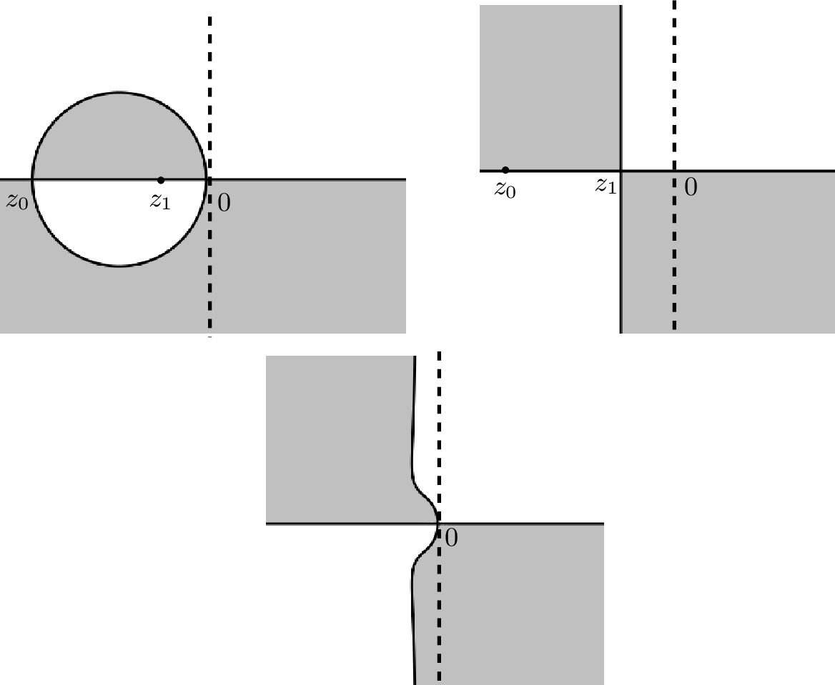
4 Long-time asymptotics in \(\mathcal{R}^{-}_{sol}\)↩︎

Since the sign of \(\xi\) affects the signature tables for phase functions \(\phi_{21}(\xi,z)\), \(\phi_{31}(\xi,z)\) and \(\phi_{32}(\xi,z)\), the contour deformation for \(\xi \in \mathcal{I}_-\) differs from that for \(\xi \in \mathcal{I}_+\). In this section, we briefly outline the overall transform procedure. Since the transformations in this section follow a similar spirit to those presented earlier, we will omit some of the details.

Throughout this section, we let \(\xi=x/(2t) \in \mathcal{I}_-\), and still denote by \(z_1=\xi\) the stationary point of the phase function \(\phi_{21}\), and by \(z_0= \frac{q_0^2}{\xi}\) the stationary point of the phase function \(\phi_{32}\). The signature tables for \(\mathop{ \mathrm{Re}}\nolimits\phi_{21}(\xi,k)\), \(\mathop{ \mathrm{Re}}\nolimits\phi_{32}(\xi,k)\) and \(\mathop{ \mathrm{Re}}\nolimits\phi_{31}(\xi,k)\) are shown in Fig. 7.

4.1 The transformations: \(\mathbf{M}\to \mathbf{M}^{(1)} \to \mathbf{M}^{(2)} \to \mathbf{M}^{(3)}\)↩︎

Our first transformation is based on the upper-lower triangular factorization of \(\mathbf{V}(x,t,z)\) (see 15 ) on the negative real axis. Let the regions \(\{\tilde{\Omega}_j \}_{j=1}^2\) be as shown in Fig. 8, and we define the transformation \(\mathbf{M}^{(1)}(x,t,z)=\mathbf{M}(x,t,z) \tilde{\mathbf{G}}(x,t,z)\), where \[\tilde{\mathbf{G}}(x,t,z)= \begin{cases} \mathrm{e}^{\Theta} \begin{pmatrix} 1&0&0\\ 0&1&0\\ 0& \frac{1}{\gamma(z)} r_3^*(z^*)&1 \end{pmatrix} \mathrm{e}^{-\Theta}, &z \in \tilde{\Omega}_1,\\ \mathrm{e}^{\Theta} \begin{pmatrix} 1&0&0\\ 0&1&-r_3(z)\\ 0& 0&1 \end{pmatrix} \mathrm{e}^{-\Theta}, &z \in \tilde{\Omega}_2,\\ \mathbf{I},& \text{elsewhere.} \end{cases}\] The jump contour \(\Gamma^{(1)}\) is illustrated in Fig. 8, and the expression for the jump matrix \(\mathbf{V}^{(1)}\) is given as follows:

\[\begin{align} &\mathbf{V}^{(1)}_2=\begin{pmatrix} 1&0&0\\ 0&1&0\\ 0& -\frac{1}{\gamma(z)} r_3^*(z^*)&1 \end{pmatrix}\mathrm{e}^{-\Theta}, \quad \mathbf{V}^{(1)}_4=\mathrm{e}^{\Theta} \begin{pmatrix} 1&0&0\\ 0&1&-r_3(z)\\ 0& 0&1 \end{pmatrix} \mathrm{e}^{-\Theta}, \\ &\mathbf{V}^{(1)}_3=\mathrm{e}^{\Theta} \begin{pmatrix} 1 & -\frac{1}{\gamma}r^*_1 & -r_2^*\\ 0 & 1 & 0\\ 0 & 0 &1 \end{pmatrix} \begin{pmatrix} 1 & 0 & 0\\ r_1&1 &0 \\ r_2&0&1 \end{pmatrix} \mathrm{e}^{-\Theta}. \end{align}\] The remaining jumps remain unchanged.

Our next transformation is designed to eliminate the \((2,1)\) and \((1,2)\) entries of the jump matrix on \((-\infty,z_1)\). Let the regions \(\{\tilde{D}_j\}_{j=1}^6\) be as shown in Fig. 9, and we define the matrix \(\mathbf{J}(x,t,z)\) as follows: \[\mathbf{J}(x,t,z)= \begin{cases} \mathrm{e}^{\Theta} \begin{pmatrix} 1&0&0\\ -r_1(z)&1&0\\ 0&0&1 \end{pmatrix}\mathrm{e}^{-\Theta} ,& z \in \tilde{D}_1 \cup \tilde{D}_2 ,\\ \mathrm{e}^{\Theta} \begin{pmatrix} 1&-\frac{1}{\gamma(z)}r^*_1(z^*)&0\\ 0&1&0\\ 0&0&1 \end{pmatrix}\mathrm{e}^{-\Theta}, & z \in \tilde{D}_5 \cup \tilde{D}_6,\\ \mathbf{I},& \text{elsewhere.} \end{cases}\] We define the second transformation as \(\mathbf{M}^{(2)}(x,t,z)=\mathbf{M}^{(1)}(x,t,z) \mathbf{J}(x,t,z)\). The jump contour \(\Gamma^{(2)}\) is depicted in Fig. 9. The expression for the associated jump matrix \(\mathbf{V}^{(2)}\) is provided below: \[\begin{align} &\mathbf{V}^{(2)}_3=\mathrm{e}^{\Theta} \begin{pmatrix} 1 &0 &0 \\ 0 & 1 & 0\\ \frac{1}{\gamma(z)} r_1(z) r_3^*(z^*) & -\frac{1}{\gamma(z)} r_3^*(z^*) &1 \end{pmatrix} \mathrm{e}^{-\Theta}, \quad \mathbf{V}^{(2)}_6=\mathrm{e}^{\Theta} \begin{pmatrix} 1& 0& -\frac{1}{\gamma(z)} r_1^*(z^*) r_3(z)\\ 0&1&-r_3(z)\\ 0&0&1 \end{pmatrix}\mathrm{e}^{-\Theta},\\ & \mathbf{V}^{(2)}_{\{2,4\}}= \mathrm{e}^{\Theta} \begin{pmatrix} 1&0&0\\ r_1(z)&1&0\\ 0& 0 &1 \end{pmatrix}\mathrm{e}^{-\Theta}, \quad \mathbf{V}^{(2)}_{\{7,8\}}=\mathrm{e}^{\Theta} \begin{pmatrix} 1&-\frac{1}{\gamma(z)} r_1^*(z^*)&0\\ 0&1&0\\ 0& 0&1 \end{pmatrix} \mathrm{e}^{-\Theta},\\ &\mathbf{V}^{(2)}_1=\mathrm{e}^{\Theta} \begin{pmatrix} 1 & 0 & -r_2^*(z^*) -\frac{1}{\gamma(z)} r_1^*(z^*) r_3(z) \\ 0 & 1 & -r_3(z)\\ 0 & 0 &1 \end{pmatrix} \begin{pmatrix} 1 & 0 & 0\\ 0&1 &0 \\ r_2(z) +\frac{1}{\gamma(z)} r_3^*(z^*) r_1(z)& -\frac{1}{\gamma(z)} r_3^*(z^*) &1 \end{pmatrix} \mathrm{e}^{-\Theta}, \\ &\mathbf{V}^{(2)}_5=\mathrm{e}^{\Theta} \begin{pmatrix} 1 & 0 & -r_2^*(z^*) \\ 0 & 1 & 0\\ 0 & 0 &1 \end{pmatrix} \begin{pmatrix} 1 & 0 & 0\\ 0&1 &0 \\ r_2(z)& 0 &1 \end{pmatrix} \mathrm{e}^{-\Theta}. \end{align}\] The remaining jumps remain unchanged.

The purpose of our third transformation is to eliminate the \((1,3)\) and \((3,1)\) elements of the jump matrix on \({\mathbb{R}}_-\). To this end, we define \(\mathbf{M}^{(3)}(x,t,z)=\mathbf{M}^{(2)}(x,t,z) \tilde{\mathbf{D}}(x,t,z)\), where \[\begin{align} \tilde{\mathbf{D}}(x,t,z)= \begin{cases} \mathrm{e}^{\Theta} \begin{pmatrix} 1 & 0 & 0\\ 0&1 &0 \\ -r_2(z)-\frac{1}{\gamma(z)}r_1(z) r_3^*(z^*)& 0 &1 \end{pmatrix} \mathrm{e}^{-\Theta},& z \in \tilde{D}_1, \\ \mathrm{e}^{\Theta} \begin{pmatrix} 1 & 0 & -r_2^*(z^*)-\frac{1}{\gamma(z)}r^*_1(z^*) r_3(z) \\ 0 & 1 & 0\\ 0 & 0 &1 \end{pmatrix}\mathrm{e}^{-\Theta},& z \in \tilde{D}_6, \\ \mathrm{e}^{\Theta} \begin{pmatrix} 1 & 0 & 0\\ 0&1 &0 \\ -r_2(z)& 0 &1 \end{pmatrix} \mathrm{e}^{-\Theta}, & z\in \tilde{D}_2 \cup \tilde{D}_3,\\ \mathrm{e}^{\Theta} \begin{pmatrix} 1 & 0 & -r_2^*(z^*)\\ 0&1 &0 \\ 0& 0 &1 \end{pmatrix} \mathrm{e}^{-\Theta}, & z\in \tilde{D}_4 \cup \tilde{D}_5,\\ \mathbf{I},& \text{elsewhere.} \end{cases} \end{align}\] The new jump contour \(\Gamma^{(3)}\) is identical to \(\Gamma^{(2)}\) except for the omission of \(\Gamma^{(2)}_5\) (see Fig. 10). The expression for the jump matrix \(\mathbf{V}^{(3)}\) is as follows: \[\begin{align} &\mathbf{V}^{(3)}_{3}=\mathrm{e}^{\Theta} \begin{pmatrix} 1&0&0\\ 0&1&0\\ 0& -\frac{1}{\gamma(z)} r_3^*(z^*) &1 \end{pmatrix}\mathrm{e}^{-\Theta}, \quad \mathbf{V}^{(3)}_{11}=\mathrm{e}^{\Theta} \begin{pmatrix} 1&0&-r_2^*(z^*)\\ 0&1&-r_3(z)\\ 0 &0&1 \end{pmatrix}\mathrm{e}^{-\Theta},\\ &\mathbf{V}^{(3)}_6= \mathrm{e}^{\Theta} \begin{pmatrix} 1 & 0 &0 \\ 0 & 1 & -r_3(z)\\ 0 & 0 &1 \end{pmatrix} \mathrm{e}^{-\Theta},\quad \mathbf{V}^{(3)}_9=\mathrm{e}^{\Theta} \begin{pmatrix} 1&0&0\\ 0&1&0\\ r_2(z) & -\frac{1}{\gamma(z)} r_3^*(z^*) &1 \end{pmatrix}\mathrm{e}^{-\Theta}, \\ &\mathbf{V}^{(3)}_1=\mathrm{e}^{\Theta} \begin{pmatrix} 1 & 0 &0 \\ 0 & 1 & -r_3(z)\\ 0 & 0 &1 \end{pmatrix} \begin{pmatrix} 1 & 0 & 0\\ 0&1 &0 \\ 0& -\frac{1}{\gamma(z)} r_3^*(z^*) &1 \end{pmatrix} \mathrm{e}^{-\Theta}, \\ &\mathbf{V}^{(3)}_{10}=\mathrm{e}^{\Theta} \begin{pmatrix} 1 & -\frac{1}{\gamma(z)} r_1^*(z^*) &0 \\ 0 & 1 &0\\ 0 & 0 &1 \end{pmatrix} \begin{pmatrix} 1 & 0 & 0\\ r_1(z)&1 &0 \\ 0&0 &1 \end{pmatrix} \mathrm{e}^{-\Theta},\quad \mathbf{V}^{(3)}_4=\mathbf{V}^{(2)}_4, \quad \mathbf{V}^{(3)}_7=\mathbf{V}^{(2)}_7, \quad \mathbf{V}^{(3)}_5=\mathbf{I}. \end{align}\]

The remaining jump matrices either remain unchanged or decay exponentially to the identity matrix \(\mathbf{I}\), and their expressions are omitted for brevity. It is also noteworthy that the three transformations performed in this subsection did not alter the residue conditions.

4.2 The transformations: \(\mathbf{M}^{(3)} \to \mathbf{M}^{(4)} \to \mathbf{M}^{(5)}\)↩︎

Similar to subsections 3.2 and 3.5, we now introduce a transformation that converts the jump matrix from an upper-lower triangular factorization to a lower-upper triangular factorization.

We first define the following diagonal matrices: \[\mathbf{\Delta^{\sharp}}=\begin{pmatrix} \delta^{\sharp}(\hat{z})& & \\ & \frac{1}{ \delta^{\sharp}(z) \delta^{\sharp}(\hat{z})}& \\ & & \delta^{\sharp}(z) \end{pmatrix},\] where \(\hat{z}=\frac{q_0^2}{z}\) and \[\label{E:deltasharp} \delta^{\sharp}(z)=\mathrm{exp} \bigg\{ \frac{1}{2 \pi \mathrm{i}} \int_{-\infty}^{z_0} \frac{\ln (1+\frac{1}{\gamma(s)}|r_3(s)|^2)}{s-z} \mathrm{d}s\bigg\}.\tag{82}\] A direct computation yields \[0< c< 1+\frac{1}{\gamma(z)}|r_3(z)|^2<1, \;\;\text{for all z \in \Gamma^{(3)}_1 and all \xi \in \mathcal{I}_-.}\] Then by the Plemelj formula, \(\delta^{\sharp}\) satisfies the following scalar RH problem: \[\begin{cases} \delta^{\sharp}_+(z)=\delta^{\sharp}_-(z) \left(1+\frac{1}{\gamma(z)}|r_3(z)|^2\right), & z \in \Gamma^{(3)}_{1},\\ \delta^{\sharp}(z) \to 1, & z \to \infty. \end{cases}\] Let \(\tilde{\delta^{\sharp}}(z)=\delta^{\sharp}(\hat{z})\), and again using the symmetry properties of \(\mathbf{A}(z)\) and \(\mathbf{B}(z)\), we find \(\tilde{\delta^{\sharp}}(z)\) satisfies the following scalar RH problem: \[\begin{cases} \tilde{\delta^{\sharp}}_+(z)=\tilde{\delta^{\sharp}}_-(z) \left(1-\frac{1}{\gamma(z)}|r_1(z)|^2\right)^{-1}, & z \in \Gamma^{(3)}_{10},\\ \tilde{\delta^{\sharp}}(z) \to \delta^{\sharp}(0), & z \to \infty. \end{cases}\] Therefore, by the Plemelj formula, \(\tilde{\delta^{\sharp}}(z)\) (i.e., \(\delta^{\sharp}(\hat{z})\)) can be written as \[\tilde{\delta^{\sharp}}(z)= \delta^{\sharp}(0) \mathrm{exp} \bigg\{ -\frac{1}{2 \pi \mathrm{i}} \int_{z_1}^{0} \frac{\ln (1-\frac{1}{\gamma(s)}|r_1(s)|^2)}{s-z} \mathrm{d}s\bigg\}.\] Further properties of \(\delta^{\sharp}(z)\) and \(\tilde{\delta^{\sharp}}(z)\) are summarized in the following lemma, which is analogous to Lemma 6.

Recall that \(\mathbf{\Delta}(z)\) is defined by 24 and \(\mathbf{P}(z)\) by 40 . Now we define the diagonal matrix \(\mathbf{T}^{\sharp}(z)= \mathbf{\Delta}(z) \mathbf{\Delta}^{\sharp}(z) \mathbf{P}(z) = \mathrm{diag}\left(T^{\sharp}_1(z), T^{\sharp}_2(z), T^{\sharp}_3(z) \right)\). The fourth transformation is defined as follows: \[\mathbf{M}^{(4)}(x,t,z)= (\mathbf{\Delta}^{\sharp}_{\infty})^{-1} (\mathbf{\Delta}^{\infty})^{-1} \mathbf{M}_{\infty}^{-1} \mathbf{M}^{(3)}(x,t,z) \mathbf{T}^{\sharp}(z),\] where \(\mathbf{\Delta}^{\sharp}_{\infty}=\mathrm{diag}\left( \delta^{\sharp}(0), \frac{1}{\delta^{\sharp}(0)},1 \right)\), \(\mathbf{\Delta}^{\infty}\) is defined in 25 , and \(\mathbf{M}^{\infty}\) is given in ?? . It is easy to see that this transformation leaves the jump contour unchanged (i.e., \(\Gamma^{(4)}=\Gamma^{(3)}\)), but we need to specify the new jump matrix. For the sake of simplicity, we only provide the expressions for the following jump matrices, which are needed in subsequent calculations: \[\begin{align} &\mathbf{V}^{(4)}_3=\mathrm{e}^{\Theta} \begin{pmatrix} 1&0&0\\ 0&1&0\\ 0& -\frac{1}{\gamma(z)} r_3^*(z^*) \frac{T_2^{\sharp}}{T_3^{\sharp}}(z)&1 \end{pmatrix}\mathrm{e}^{-\Theta}, \quad \mathbf{V}^{(4)}_6=\mathrm{e}^{\Theta} \begin{pmatrix} 1&0&0\\ 0&1&-r_3(z)\frac{T_3^{\sharp}}{T_2^{\sharp}}(z)\\ 0& 0&1 \end{pmatrix} \mathrm{e}^{-\Theta},\\ &\mathbf{V}^{(4)}_{4}=\mathrm{e}^{\Theta} \begin{pmatrix} 1&0&0\\ r_1(z) \frac{T_1^{\sharp}}{T^{\sharp}_2}(z)&1&0\\ 0&0&1 \end{pmatrix}\mathrm{e}^{-\Theta}, \quad \mathbf{V}^{(4)}_7= \mathrm{e}^{\Theta} \begin{pmatrix} 1 & -\frac{1}{\gamma(z)} r_1^*(z^*) \frac{T_2^{\sharp}}{T_1^{\sharp}}(z) &0 \\ 0 & 1 & 0\\ 0 & 0 &1 \end{pmatrix} \mathrm{e}^{-\Theta},\\ &\mathbf{V}^{(4)}_{10}=\mathrm{e}^{\Theta} \begin{pmatrix} 1& 0 & 0\\ \frac{r_1(z)}{1-\frac{1}{\gamma(z)} |r_1(z)|^2} \frac{T_{1-}^{\sharp}}{T_{2-}^{\sharp}}& 1 & 0\\ 0& 0 &1 \end{pmatrix} \begin{pmatrix} 1& -\frac{1}{\gamma(z)} \frac{r_1^*(z)}{1-\frac{1}{\gamma(z)} |r_1(z)|^2} \frac{T_{2+}^{\sharp}}{T_{1+}^{\sharp}}& 0\\ 0 & 1 & 0\\ 0 & 0 &1 \end{pmatrix} \mathrm{e}^{-\Theta},\\ &\mathbf{V}^{(4)}_{1}=\mathrm{e}^{\Theta} \begin{pmatrix} 1& 0 & 0\\ 0& 1 & 0\\ 0& -\frac{1}{\gamma(z)} \frac{r_3^*(z)}{1+\frac{1}{\gamma(z)} |r_3(z)|^2} \frac{T_{2-}^{\sharp}}{T_{3-}^{\sharp}} &1 \end{pmatrix} \begin{pmatrix} 1& 0& 0\\ 0 & 1 & - \frac{r_3(z)}{1+\frac{1}{\gamma(z)} |r_3(z)|^2} \frac{T_{3+}^{\sharp}}{T_{2+}^{\sharp}}\\ 0 & 0 &1 \end{pmatrix} \mathrm{e}^{-\Theta},\\ &\mathbf{V}^{(4)}_{12}=(\mathbf{\Delta}^{\sharp} \mathbf{P})^{-1}(z) \mathrm{e}^{\Theta} \begin{pmatrix} 1 & 0 &0 \\ -\tilde{r}_1 &1 &0 \\ \tilde{r}_2 & \frac{1}{\gamma}\tilde{r}_3^* &1 \end{pmatrix} \begin{pmatrix} 1 &\frac{1}{\gamma}\tilde{r}_1^* & -\tilde{r}_2^*\\ 0 & 1 & \tilde{r}_3\\ 0&0 &1 \end{pmatrix} \mathrm{e}^{-\Theta} \mathbf{\Delta}^{\sharp}(z) \mathbf{P}(z),\\ &\mathbf{V}^{(4)}_{9}=(\mathbf{T}^{\sharp})^{-1} \mathbf{V}^{(3)}_{9} \mathbf{T}^{\sharp}, \quad \mathbf{V}^{(4)}_{11}=(\mathbf{T}^{\sharp})^{-1} \mathbf{V}^{(3)}_{11} \mathbf{T}^{\sharp}. \end{align}\]

In the last expression above, \(\{ \tilde{r}_j(z)\}_{j=1}^3\) is given by 30 . Furthermore, Let \(\{\tilde{U}_j \}_{j=1}^7\) denote the regions shown in Fig. 11. We define the matrices \[\begin{align} &(\mathbf{V}^{(4)}_{12})^L= (\mathbf{\Delta}^{\sharp} \mathbf{P})^{-1} (z) \mathrm{e}^{\Theta} \begin{pmatrix} 1 & 0 &0 \\ -\tilde{r}_1(z) &1 &0 \\ \tilde{r}_2(z) & \frac{1}{\gamma}\tilde{r}_3^*(z^*) &1 \end{pmatrix}\mathrm{e}^{-\Theta} \mathbf{\Delta}^{\sharp}(z) \mathbf{P}(z), \qquad z \in \tilde{U}_4;\\ &(\mathbf{V}^{(4)}_{12})^U=(\mathbf{\Delta}^{\sharp} \mathbf{P})^{-1}(z) \mathrm{e}^{\Theta} \begin{pmatrix} 1 &\frac{1}{\gamma}\tilde{r}_1^* (z^*) & -\tilde{r}_2^*(z^*)\\ 0 & 1 & \tilde{r}_3(z)\\ 0&0 &1 \end{pmatrix} \mathrm{e}^{-\Theta} \mathbf{\Delta}^{\sharp}(z) \mathbf{P}(z), \qquad z \in \tilde{U}_3;\\ &(\mathbf{V}^{(4)}_{10})^U=\mathrm{e}^{\Theta} \begin{pmatrix} 1& -\frac{1}{\gamma(z)} \frac{r_1^*(z^*)}{1-\frac{1}{\gamma(z)} r_1(z) r_1^*(z^*)} \frac{T_{2}^{\sharp}}{T_{1}^{\sharp}}(z)& 0\\ 0 & 1 & 0\\ 0 & 0 &1 \end{pmatrix} \mathrm{e}^{-\Theta}, \qquad z \in \tilde{U}_2 ; \\ &(\mathbf{V}^{(4)}_{10})^L=\mathrm{e}^{\Theta} \begin{pmatrix} 1& 0 & 0\\ \frac{r_1(z)}{1-\frac{1}{\gamma(z)} r_1(z) r_1^*(z^*)} \frac{T_{1}^{\sharp}}{T_{2}^{\sharp}}(z)& 1 & 0\\ 0& 0 &1 \end{pmatrix} \mathrm{e}^{-\Theta}, \qquad z \in \tilde{U}_5 \cup \tilde{U}_7;\\ &(\mathbf{V}^{(4)}_{1})^U= \mathrm{e}^{\Theta} \begin{pmatrix} 1& 0& 0\\ 0 & 1 & - \frac{r_3(z)}{1+\frac{1}{\gamma(z)} r_3(z) r_3^*(z^*)} \frac{T_{3}^{\sharp}}{T_{2}^{\sharp}}(z)\\ 0 & 0 &1 \end{pmatrix} \mathrm{e}^{-\Theta}, \qquad z\in \tilde{U}_1;\\ &(\mathbf{V}^{(4)}_{1})^L=\mathrm{e}^{\Theta} \begin{pmatrix} 1& 0 & 0\\ 0& 1 & 0\\ 0& -\frac{1}{\gamma(z)} \frac{r_3^*(z^*)}{1+\frac{1}{\gamma(z)} r_3(z) r_3^*(z^*)} \frac{T_{2}^{\sharp}}{T_{3}^{\sharp}} &1 \end{pmatrix}\mathrm{e}^{-\Theta}, \qquad z \in \tilde{U}_6 \end{align}\] so that \(\mathbf{V}^{(4)}_{12}\), \(\mathbf{V}^{(4)}_1\) and \(\mathbf{V}^{(4)}_{10}\) can be rewritten as \[\mathbf{V}^{(4)}_{12}=(\mathbf{V}^{(4)}_{12})^L (\mathbf{V}^{(4)}_{12})^U, \qquad \mathbf{V}^{(4)}_1= (\mathbf{V}^{(4)}_1)^L (\mathbf{V}^{(4)}_1)^U, \qquad (\mathbf{V}^{(4)}_{10})=(\mathbf{V}^{(4)}_{10})^L (\mathbf{V}^{(4)}_{10})^U.\]

We are now ready to define our fifth transformation. We let \(\mathbf{M}^{(5)}(x,t,z)=\mathbf{M}^{(4)}(x,t,z) \tilde{\mathbf{N}}(x,t,z)\), where \[\tilde{\mathbf{N}}(x,t,z)=\begin{cases} \left( (\mathbf{V}^{(4)}_{1})^U (x,t,z)\right)^{-1}, & z \in \tilde{U}_1,\\ (\mathbf{V}^{(4)}_{1})^L(x,t,z), & z \in \tilde{U}_6,\\ \left( (\mathbf{V}^{(4)}_{10})^U (x,t,z) \right)^{-1}, & z\in \tilde{U}_2,\\ (\mathbf{V}^{(4)}_{10})^L (x,t,z),& z \in \tilde{U}_5 \cup \tilde{U}_7,\\ \left((\mathbf{V}^{(4)}_{12})^U(x,t,z) \right)^{-1}, & z \in \tilde{U}_3,\\ (\mathbf{V}^{(4)}_{12})^L(x,t,z), & z \in \tilde{U}_4,\\ \mathbf{I},& \text{elsewhere.} \end{cases}\] The jump contour \(\Gamma^{(5)}\) is illustrated in Figure 11. We provide the exact expressions for the following jump matrices: \[\begin{align} &\mathbf{V}^{(5)}_1= \mathbf{V}^{(4)}_3, \quad \mathbf{V}^{(5)}_2=(\mathbf{V}^{(4)}_{1})^U, \quad \mathbf{V}^{(5)}_3=(\mathbf{V}^{(4)}_{1})^L, \quad \mathbf{V}^{(5)}_4=\mathbf{V}^{(4)}_6; \\ & \mathbf{V}^{(5)}_5=(\mathbf{V}^{(4)}_{10})^U, \quad \mathbf{V}^{(5)}_8=(\mathbf{V}^{(4)}_{10})^L \quad \mathbf{V}^{(5)}_{6}=\mathbf{V}^{(4)}_4, \quad \mathbf{V}^{(5)}_{7}=\mathbf{V}^{(4)}_{7};\\ &\mathbf{V}^{(5)}_9=(\mathbf{V}^{(4)}_{12})^U, \quad \mathbf{V}^{(5)}_{10}=(\mathbf{V}^{(4)}_{12})^U \mathbf{V}^{(4)}_{9}, \quad \mathbf{V}^{(5)}_{11}=\left( (\mathbf{V}^{(4)}_{10})^L\right)^{-1} \mathbf{V}^{(4)}_{11} (\mathbf{V}^{(4)}_{10})^L, \\ &\mathbf{V}^{(5)}_{12}=\left( (\mathbf{V}^{(4)}_{10})^L\right)^{-1} (\mathbf{V}^{(4)}_{12})^L. \end{align}\] We then have the following lemma, which is similar to Lemma 9, and hence its proof is omitted.

Using this lemma, one can easily prove that \(\mathbf{V}^{(5)}\) converges to the identity matrix \(\mathbf{I}\) as \(t \to \infty\) uniformly for \(\xi \in \mathcal{I}_-\) and \(z \in \Gamma^{(5)}\) except near the two critical points \(z_0\) and \(z_1\). Hence, the behavior in the vicinity of the critical point is crucial, and we will next construct a local model to approximate it.

4.3 The outer parametrix and the local parametrix↩︎

We now construct a outer parametrix that satisfies the same residue conditions as \(\mathbf{M}^{(5)}\). To achieve this, we consider the following modulated pure-soliton RH problem:

If \(\frac{\tau_j}{\zeta_j}<0\) holds for all \(0 \leq j \leq N-1\), then the solution to above RH problem exists and is unique for each \((x,t) \in {\mathbb{R}}\times {\mathbb{R}}_+\). The proof of this assertion can be followed exactly as in the proof of Lemma 11. We define the function \(\mathbf{M}^{out}_{\sharp}\) as \[\label{E:Mshout} \mathbf{M}^{out}_{\sharp}(x,t,z)=(\mathbf{M}_{\infty})^{-1}\mathbf{M}^{\sharp}_{msol}(x,t,z) \mathbf{P}(z),\tag{83}\] where \(\mathbf{P}(z)\) is given by 40 . The function \(\mathbf{M}^{out}_{\sharp}\) serves as the outer parametrix we require, because it satisfies the same residue conditions as \(\mathbf{M}^{(5)}\).

Next, we proceed to construct the local models. Let the notation \(D_{\epsilon }(z_0)\), \(D_{\epsilon }(z_1)\), \(\mathcal{D}\), \(\partial \mathcal{D}\), \(X^{R,\epsilon}_j\), \(X^{L,\epsilon}_j\) and \(X^{\epsilon}\) denote the same meaning as in subsection 3.6. Then we introduce the new variables \(y_{\ell}\) and \(y_{r}\), which are the same as those in subsection 3.6; see 47 . Recalling the definition of \(\mathbf{T}^{\sharp}\), we have \[\frac{T_2^{\sharp}}{T_3^{\sharp}}(z)=\frac{ 1 }{(\delta^{\sharp}(z))^2 \delta^{\sharp}(\hat{z}) \delta_1^2(\hat{z})\delta_1(z) \mathcal{P}^2_1(\hat{z}) \mathcal{P}_1(z) },\quad \frac{T_1^{\sharp}}{T_2^{\sharp}}(z)= \delta_1(\hat{z})\delta^2_1(z) \mathcal{P}_1(\hat{z}) \mathcal{P}_1^2(z) (\delta^{\sharp}(\hat{z}))^2 \delta^{\sharp}(z).\] Then ?? and 47 imply that, for \(\xi \in \mathcal{I}_-\) \[\begin{align} & \frac{T_2^{\sharp}}{T_3^{\sharp}}(z)=\mathrm{e}^{-2 \mathrm{i}\nu^{\sharp} \log_{\pi} y_r} \hbar _0 \hbar_1(z), \qquad z \in D_{\epsilon}(z_0) \setminus (-\infty, z_0],\\ &\frac{T_1^{\sharp}}{T_2^{\sharp}}(z)=\mathrm{e}^{2 \mathrm{i}\nu^{\sharp} \log_{0} y_{\ell}} h_0 h_1(z), \qquad z \in D_{\epsilon}(z_1) \setminus [z_1,0), \end{align}\] where \[\begin{align} &\hbar_0=\left( \frac{q_0^2}{\xi^2 \sqrt{2t}} \right)^{-2 \mathrm{i}\nu^{\sharp}}\frac{ \mathrm{e}^{2 \chi^{\sharp}(z_0)} }{ \delta^{\sharp}(z_1) \delta_1^2(z_1)\delta_1(z_0) \mathcal{P}_1^2(z_1) \mathcal{P}_1(z_0) },\\ &\hbar_1(z)=\frac{\delta^{\sharp}(z_1) \delta_1^2(z_1)\delta_1(z_0) \mathcal{P}_1^2(z_1) \mathcal{P}_1(z_0)}{\delta^{\sharp}(\hat{z}) \delta_1^2(\hat{z})\delta_1(z) \mathcal{P}_1^2(\hat{z}) \mathcal{P}_1(z) } \mathrm{e}^{2 \chi^{\sharp}-2 \chi^{\sharp}(z_0) },\\ &h_0=(\sqrt{2t})^{-2 \mathrm{i}\nu^{\sharp} } (\delta^{\sharp}(0))^2 \delta^{\sharp}(z_1) \delta_1(z_0)\delta_1^2(z_1) \mathcal{P}_1(z_0) \mathcal{P}^2_1(z_1) \mathrm{e}^{-2 \tilde{\chi}^{\sharp}(z_1) },\\ &h_1(z)=\frac{\delta^{\sharp}(z) \delta_1(\hat{z})\delta^2_1(z) \mathcal{P}_1(\hat{z}) \mathcal{P}^2_1(z) }{ \delta^{\sharp}(z_1) \delta_1(z_0)\delta_1^2(z_1) \mathcal{P}_1(z_0) \mathcal{P}^2_1(z_1)} \mathrm{e}^{2 \tilde{\chi}^{\sharp}(z_1)-2 \tilde{\chi}^{\sharp}(z) }. \end{align}\] we define \[\label{E:Ysh} \mathbf{Y}^{\sharp}(\xi,t)=\begin{cases} \mathbf{Y}_L^{\sharp}(\xi,t), &z \in D_{\epsilon}(z_1),\\ \mathbf{Y}_R^{\sharp}(\xi,t), & z \in D_{\epsilon}(z_0), \end{cases}\tag{84}\] where \[\begin{align} &\mathbf{Y}_R^{\sharp}(\xi,t)=\begin{pmatrix} 1& &\\ & \hbar_0^{-1/2}\mathrm{e}^{-\frac{\theta_{32}(x,t,z_0)}{2}}&\\ & & \hbar_0^{1/2}\mathrm{e}^{\frac{\theta_{32}(x,t,z_0)}{2}} \end{pmatrix}, \\ &\mathbf{Y}_L^{\sharp}(\xi,t)=\begin{pmatrix} h_0^{-1/2}\mathrm{e}^{-\frac{\theta_{21}(x,t,z_1)}{2}}& &\\ &h_0^{1/2}\mathrm{e}^{\frac{\theta_{21}(x,t,z_1)}{2}} &\\ & & 1 \end{pmatrix}. \end{align}\] Through a discussion entirely analogous to that in subsection 3.6, one can prove that \(\mathbf{M}^{\sharp}_{loc}\), defined by \[\label{E:Mloc-1} \mathbf{M}_{loc}^{\sharp}(x,t,z)=\begin{cases} \mathbf{Y}_L^{\sharp}(\xi,t) \mathbf{N}^{X,L}(x,t,z) (\mathbf{Y}_L^{\sharp})^{-1}(\xi,z), & z \in D_{\epsilon}(z_1),\\ \mathbf{Y}_R^{\sharp}(\xi,t) \mathbf{N}^{X,R}(x,t,z) (\mathbf{Y}_R^{\sharp})^{-1}(\xi,z), & z \in D_{\epsilon}(z_0), \end{cases}\tag{85}\] well-approximates \(\mathbf{M}^{(5)}(x,t,z)\) within the region \(\mathcal{D}\). Here, \(\mathbf{N}^{X,L}(x,t,z)\) and \(\mathbf{N}^{X,R}(x,t,z)\) are the solutions to the model RH problem defined in Appendix 9.2. More precisely, we have the following result.

4.4 Final Transformation: \(\mathbf{M}^{(5)} \to \boldsymbol{\mathcal{E}}\)↩︎

The final transformation is defined as follows: \[\label{E:defEA} \boldsymbol{\mathcal{E}}(x,t,z)=\begin{cases} \mathbf{M}^{(5)}(x,t,z)(\mathbf{M}_{loc}^{\sharp})^{-1}(x,t,z)(\mathbf{M}^{out}_{\sharp})^{-1}(x,t,z), &z \in \mathcal{D},\\ \mathbf{M}^{(5)}(x,t,z)(\mathbf{M}^{out}_{\sharp})^{-1}(x,t,z), & z\in \mathbb{C}\setminus \mathcal{D}, \end{cases}\tag{86}\] where \(\mathbf{M}^{out}_{\sharp}\) and \(\mathbf{M}_{loc}^{\sharp}\) are defined by 83 and 85 , respectively. As in subsection 3.7, one can show that \(\boldsymbol{\mathcal{E}}(x,t,z)\) defined by 86 has a well-defined limit at \(z_{\sharp}\), where \(z_{\sharp} \in \{ 0, \pm q_0\} \cup \{ \zeta_j \}_{j=0}^{N-1} \cup \{\zeta_j^* \}_{j=0}^{N-1}\). Let \(\Gamma^{\mathcal{E}}=\Gamma^{(5)} \cup \partial \mathcal{D}\), then \(\boldsymbol{\mathcal{E}}\) satisfies the following RH problem:

Moreover, let \(\boldsymbol{\omega}^{\mathcal{E}}=\mathbf{V}^{\mathcal{E}}-\mathbf{I}\) , then we have the following result similar to Lemma 16.

The estimates in Lemma 21 show that \[\begin{align} \begin{cases} \|\boldsymbol{\omega}^{\mathcal{E}}\|_{L^1 (\Gamma^{\mathcal{E}})} \leq C t^{-1}\ln t\\ \|\boldsymbol{\omega}^{\mathcal{E}}\|_{L^{\infty} (\Gamma^{\mathcal{E}})} \leq C t^{-1/2}\ln t \end{cases} \qquad \xi \in \mathcal{I}_-, \;\;t>2. \end{align}\] Therefore, analogous to the case in subsection 3.7, RH problem 22 is a small-norm problem and is therefore uniquely solvable for sufficiently large \(t\). Now, let the Cauchy operator associated with the contour \(\Gamma^{\epsilon}\) be denoted by \(\mathcal{C}\), and define the operator \(\mathcal{C}_{\boldsymbol{\omega}^{\mathcal{E}}}\) as \(\mathcal{C}_{\boldsymbol{\omega}^{\mathcal{E}}}(\mathbf{h})=\mathcal{C}_-(\mathbf{h}\boldsymbol{\omega}^{\mathcal{E}})\) for any \(\mathbf{h}\in L^2(\Gamma^{\epsilon})\). Moreover, let the function \(\boldsymbol{\mu}^{\mathcal{E}}\) be defined as \[\boldsymbol{\mu}^{\mathcal{E}}=\mathbf{I}+(I-\mathcal{C}_{\boldsymbol{\omega}^{\mathcal{E}}})^{-1}\mathcal{C}_{\boldsymbol{\omega}^{\mathcal{E}}}\mathbf{I}\;\in \mathbf{I}+ L^2(\Gamma^{\mathcal{E}}).\] Following the discussion in subsection 3.7, it can be shown that the above definitions are well-defined, and \(\boldsymbol{\mathcal{E}}(x,t,z)\) can be expressed as \[\label{E:Ejfbs-1} \boldsymbol{\mathcal{E}}(x,t,z)=\mathbf{I}+\frac{1}{2\pi \mathrm{i}}\int_{\Gamma^{\mathcal{E}}}\frac{\boldsymbol{\mu}^{\mathcal{E}}(z') \boldsymbol{\omega}^{\mathcal{E}}(z')dz'}{z'-z}.\tag{87}\] Therefore, the non-tangential limit \[\boldsymbol{\mathcal{E}}^{(1)}(x,t)= \lim^{\angle}(\boldsymbol{\mathcal{E}}(x,t,z)-\mathbf{I})=-\frac{1}{2\pi \mathrm{i}}\int_{\Gamma^{\mathcal{E}}}\boldsymbol{\mu}^{\mathcal{E}} (x,t,\zeta)\boldsymbol{\omega}^{\mathcal{E}}(x,t,\zeta) \mathrm{d}\zeta,\] is well-defined. We have the following estimate for \(\boldsymbol{\mathcal{E}}^{(1)}(x,t)\), the proof of which is closely analogous to that of Lemma 17, and therefore we omit it.

Then we define the functions \(F^{(1)}_{\sharp}(\xi,t)\) and \(F^{(2)}_{\sharp}(\xi,t)\) by \[F^{(1)}_{\sharp}(\xi,t)=-\frac{1}{2\pi \mathrm{i}} \int_{\partial D_{\epsilon}(z_0)} \boldsymbol{\omega}^{\mathcal{E}}(x,t,\zeta) \mathrm{d} \zeta, \qquad F^{(2)}_{\sharp}(\xi,t)=-\frac{1}{2\pi \mathrm{i}} \int_{\partial D_{\epsilon}(z_1)} \boldsymbol{\omega}^{\mathcal{E}}(x,t,\zeta) \mathrm{d} \zeta.\] Recalling the definitions of \(\boldsymbol{\omega}^{\mathcal{E}}\), \(\mathbf{M}^{out}_{\sharp}\), \(\mathbf{Y}_L^{\sharp}\), \(\mathbf{Y}_R^{\sharp}\), \(\mathbf{N}^{X,L}_{\infty}\) and \(\mathbf{N}^{X,R}_{\infty}\), using ?? and applying the residue theorem, we obtain \[\begin{align} F^{(1)}_{\sharp}(\xi,t)&=\frac{q_0^2}{\xi^2 \sqrt{2t}} \mathbf{M}_{\infty}^{-1} \mathbf{M}^{\sharp}_{msol}(x,t,z_0) \mathbf{Z}_R^{\sharp}(\xi,t) (\mathbf{M}_{msol}^{\sharp})^{-1}(x,t,z_0) \mathbf{M}_{\infty}+\mathcal{O}(t^{-1}), \qquad t \to \infty,\\ F^{(2)}_{\sharp}(\xi,t)&=\frac{1}{\sqrt{2t}} \mathbf{M}_{\infty}^{-1} \mathbf{M}_{msol}^{\sharp}(x,t,z_1) \mathbf{Z}_L^{\sharp}(\xi,t) (\mathbf{M}_{msol}^{\sharp})^{-1}(x,t,z_1) \mathbf{M}_{\infty}+\mathcal{O}(t^{-1}), \qquad t \to \infty. \end{align}\] Here \[\label{E:ZRZLsha} \mathbf{Z}_L^{\sharp}=\begin{pmatrix} 0&\mathrm{i}\tilde{\beta}_{12}(\tilde{h}_0)^{-1}\mathrm{e}^{\theta_{12}(z_1)}&0\\ -\mathrm{i}\tilde{\beta}_{21} \tilde{h}_0 \mathrm{e}^{\theta_{21}(z_1)} &0 &0\\ 0&0&0 \end{pmatrix}, \mathbf{Z}_R^{\sharp}= \begin{pmatrix} 0&0&0\\ 0&0&-\mathrm{i}\tilde{\beta}_{23} (\tilde{\hbar}_0)^{-1} \mathrm{e}^{\theta_{23}(z_0)}\\ 0& \mathrm{i}\tilde{\beta}_{32} \tilde{\hbar}_0 \mathrm{e}^{\theta_{32}(z_0)}&0 \end{pmatrix},\tag{88}\] where \[\label{E:d0tilA} \begin{align} &\tilde{\hbar}_0= \hbar_0 \mathcal{P}^2_1(z_0) \mathcal{P}_1(z_1)=\left( \frac{q_0^2}{\xi^2 \sqrt{2t}} \right)^{-2 \mathrm{i}\nu^{\sharp}}\frac{ \mathrm{e}^{2 \chi^{\sharp}(z_0)} }{ \delta^{\sharp}(z_1) \delta_1^2(z_1)\delta_1(z_0) },\\ &\tilde{h}_0= \frac{h_0}{\mathcal{P}_1^2(z_0) \mathcal{P}_1(z_1)}=(\sqrt{2t})^{-2 \mathrm{i}\nu^{\sharp} } (\delta^{\sharp}(0))^2 \delta^{\sharp}(z_1) \delta_1(z_0)\delta_1^2(z_1) \mathrm{e}^{-2 \tilde{\chi}^{\sharp}(z_1) }, \end{align}\tag{89}\] and \(\tilde{\beta}_{12}\), \(\tilde{\beta}_{21}\), \(\tilde{\beta}_{23}\) and \(\tilde{\beta}_{32}\) are given by 126 . Thus we have \[\label{E:estofL-A} \begin{align} \boldsymbol{\mathcal{E}}^{(1)}(x,t)&=\frac{q_0^2}{\xi^2 \sqrt{2t}} \mathbf{M}_{\infty}^{-1} \mathbf{M}_{msol}^{\sharp}(x,t,z_0) \mathbf{Z}_R^{\sharp}(\xi,t) (\mathbf{M}_{msol}^{\sharp})^{-1}(x,t,z_0) \mathbf{M}_{\infty}\\ &+\frac{1}{\sqrt{2t}} \mathbf{M}_{\infty}^{-1} \mathbf{M}_{msol}^{\sharp}(x,t,z_1) \mathbf{Z}_L^{\sharp}(\xi,t) (\mathbf{M}_{msol}^{\sharp})^{-1}(x,t,z_1) \mathbf{M}_{\infty} +\mathcal{O}(t^{-1} \ln t). \end{align}\tag{90}\]

4.5 Proof of the asymptotic formula ??↩︎

Taking into account all the transformations we have performed in this section, we obtain \[\begin{align} \label{E:alltranA} \boldsymbol{\mathcal{E}}(x,t,z)=(\mathbf{\Delta}_{\infty}^{\sharp} \mathbf{\Delta}^{\infty})^{-1} (\mathbf{M}_{\infty})^{-1} \mathbf{M}(x,t,z) \mathbf{T}^{\sharp}(z) (\mathbf{M}_{msol}^{\sharp} \mathbf{P})^{-1}(x,t,z) \mathbf{M}_{\infty}, \end{align}\tag{91}\] where we have selected \(z\) such that \(\tilde{\mathbf{G}}(z)=\mathbf{J}(z)=\tilde{\mathbf{D}}(z)=\tilde{\mathbf{N}}(z)=\mathbf{I}\). Hence we have \[\label{E:czA} \mathbf{M}(x,t,z)=\mathbf{M}_{\infty} \mathbf{\Delta}^{\infty}\mathbf{\Delta}_{\infty}^{\sharp} \boldsymbol{\mathcal{E}}(x,t,z)(\mathbf{M}_{\infty})^{-1} \mathbf{M}_{msol}^{\sharp}(x,t,z) \mathbf{P}(z)(\mathbf{T}^{\sharp}(z))^{-1} .\tag{92}\] Recall the reconstruction formula \[\label{E:fcggsA} \mathbf{q}(x,t)=- \mathrm{i}\lim_{z \to \infty}z \mathbf{m}_{rc}(x,t,z), \qquad \mathbf{m}_{rc}=(\mathbf{M}_{21}, \mathbf{M}_{31})^{\top}.\tag{93}\] Therefore, we need to examine the asymptotic behavior of the functions on the right-hand side of Eq. 92 as \(z \to \infty\). We can easily obtain that as \(z \to \infty\), \[\begin{align} &\boldsymbol{\mathcal{E}}(x,t,z)=\mathbf{I}+\frac{1}{z} \boldsymbol{\mathcal{E}}^{(1)}(x,t)+\mathcal{O}(\frac{1}{z^2}),\\ &\mathbf{M}_{msol}(x,t,z)=\mathbf{M}_{\infty}+\frac{1}{z} (\mathbf{M}^{\sharp}_{msol})^{(1)}(x,t)+\mathcal{O}(\frac{1}{z^2}),\\ &\mathbf{P}(z) (\mathbf{T}^{\sharp}(z))^{-1}=(\mathbf{\Delta}_{\infty}^{\sharp})^{-1} (\mathbf{\Delta}^{\infty})^{-1}+\frac{1}{z} \mathbf{C}^{\sharp} + \mathcal{O}(\frac{1}{z^2}), \end{align}\] where \(\mathbf{C}^{\sharp}\) is a diagonal matrix. Then, by substituting the above asymptotic expansions into 92 and combining with reconstruction formula 93 , we have \[\label{E:zzzzz} \mathbf{q}(x,t)= \check{\mathbf{M}}_\infty \boldsymbol{\sigma}^{\sharp} \check{\mathbf{M}}_\infty^{-1} \begin{pmatrix} -\mathrm{i}(\mathbf{M}_{msol}^{\sharp})^{(1)}_{21} \\ -\mathrm{i}(\mathbf{M}_{msol}^{\sharp})^{(1)}_{31} \end{pmatrix}+ \check{\mathbf{M}}_\infty \boldsymbol{\sigma}^{\sharp} \begin{pmatrix} - \mathrm{i}\boldsymbol{\mathcal{E}}^{(1)}_{21}\\ -\mathrm{i}\boldsymbol{\mathcal{E}}^{(1)}_{31} \end{pmatrix},\tag{94}\] where \[\label{E:cheMandsiAA} \check{\mathbf{M}}_\infty=\begin{pmatrix} \frac{q_{2,+}^*}{q_0} & \frac{q_{1,+}}{q_0}\\ -\frac{q_{1,+}^*}{q_0} &\frac{q_{2,+}}{q_0} \end{pmatrix}, \qquad \boldsymbol{\sigma}^{\sharp}=\begin{pmatrix} \frac{1}{(\delta^{\sharp}(0))^2\delta_1(0) } & \\ & \frac{\delta_1(0) }{\delta^{\sharp}(0)} \end{pmatrix}.\tag{95}\] Let us define \(\tilde{\mathbf{q}}^{[N]}_{msol}\) as \[\label{E:ansol} \tilde{\mathbf{q}}^{[N]}_{msol}(x,t)=\check{\mathbf{M}}_\infty \boldsymbol{\sigma}^{\sharp} \check{\mathbf{M}}_\infty^{-1} \begin{pmatrix} -\mathrm{i}(\mathbf{M}_{msol}^{\sharp})^{(1)}_{21} \\ -\mathrm{i}(\mathbf{M}_{msol}^{\sharp})^{(1)}_{31} \end{pmatrix}.\tag{96}\] Moreover, since \(\check{\mathbf{M}}_\infty \boldsymbol{\sigma}^{\sharp} \check{\mathbf{M}}_\infty^{-1}\) is a unitary matrix, \(\tilde{\mathbf{q}}^{[N]}_{msol}(x,t)\) is the solution of the defocusing Manakov system 1 . We still refer to it as the modulated \(N\)-soliton.

Now, let us consider the second term on the right-hand side of Eq 94 . First, we have \[\check{\mathbf{M}}_\infty \boldsymbol{\sigma}^{\sharp} \begin{pmatrix} -\mathrm{i}\boldsymbol{\mathcal{E}}^{(1)}_{21} \\ -\mathrm{i}\boldsymbol{\mathcal{E}}^{(1)}_{31} \end{pmatrix}= \begin{pmatrix} \left(\frac{|q_{2,+}|^2 }{q_0^2 (\delta^{\sharp}(0))^2\delta_1(0) }+\frac{|q_{1,+}|^2 }{q_0^2 } \frac{\delta_1(0)}{\delta^{\sharp}(0)}\right) \tilde{\boldsymbol{\mathcal{E}}}^{(1)}_{21}+ \frac{q_{1,+} q_{2,+}^* }{q_0^2} \left(\frac{\delta_1(0)}{\delta^{\sharp}(0)}-\frac{1}{(\delta^{\sharp}(0))^2\delta_1(0) }\right) \tilde{\boldsymbol{\mathcal{E}}}^{(1)}_{31}\\ \left(\frac{|q_{1,+}|^2 }{q_0^2 (\delta^{\sharp}(0))^2\delta_1(0) } +\frac{|q_{2,+}|^2 }{q_0^2 } \frac{\delta_1(0)}{\delta^{\sharp} (0)} \right) \tilde{\boldsymbol{\mathcal{E}}}^{(1)}_{31}+ \frac{q_{2,+} q_{1,+}^* }{q_0^2} \left(\frac{\delta_1(0)}{\delta^{\sharp}(0)}- \frac{1}{\delta^{\sharp}(0))^2\delta_1(0) }\right) \tilde{\boldsymbol{\mathcal{E}}}^{(1)}_{21} \end{pmatrix},\] where \[\begin{pmatrix} \tilde{\boldsymbol{\mathcal{E}}}^{(1)}_{21}\\ \tilde{\boldsymbol{\mathcal{E}}}^{(1)}_{31} \end{pmatrix} = \check{\mathbf{M}}_\infty \begin{pmatrix} -\mathrm{i}\boldsymbol{\mathcal{E}}^{(1)}_{21} \\ -\mathrm{i}\boldsymbol{\mathcal{E}}^{(1)}_{31} \end{pmatrix}.\] Then we proceed to estimate \(\tilde{\boldsymbol{\mathcal{E}}}^{(1)}_{21}(x,t)\) and \(\tilde{\boldsymbol{\mathcal{E}}}^{(1)}_{31}(x,t)\). From 90 , one can obtain \[\tilde{\boldsymbol{\mathcal{E}}}^{(1)}_{21}(x,t)=\frac{L_A^{\sharp}(x,t)}{\sqrt{t}}+\mathcal{O}(t^{-1} \ln t), \qquad \tilde{\boldsymbol{\mathcal{E}}}^{(1)}_{31}(x,t)=\frac{L_B^{\sharp}(x,t)}{\sqrt{t}}+\mathcal{O}(t^{-1} \ln t),\] where \[\begin{align} L_A^{\sharp}(x,t)&=\frac{q_0^2}{\xi^2 \sqrt{2}} \bigg[ \tilde{\beta}_{23}\tilde{\hbar}_0 \mathrm{e}^{\theta_{32}(z_0)} \left( \mathbf{M}^{\sharp}_{msol}(x,t,z_0) \right)_{23} \left( (\mathbf{M}_{msol}^{\sharp})^{-1}(x,t,z_0) \right)_{21} \tag{97}\\ &- \tilde{\beta}_{23}(\tilde{\hbar}_0)^{-1} \mathrm{e}^{\theta_{23}(z_0)}\left( \mathbf{M}_{msol}^{\sharp} (x,t,z_0)\right)_{22} \left( (\mathbf{M}_{msol}^{\sharp})^{-1}(x,t,z_0) \right)_{31} \bigg] \nonumber\\ &+ \frac{1}{\sqrt{2}} \bigg[- \tilde{\beta}_{21}\tilde{h}_0 \mathrm{e}^{\theta_{21}(z_1)}\left( \mathbf{M}_{msol}^{\sharp} (x,t,z_1)\right)_{22}\left( (\mathbf{M}_{msol}^{\sharp})^{-1}(x,t,z_1) \right)_{11} \nonumber\\ &+ \tilde{\beta}_{12}(\tilde{h}_0)^{-1} \mathrm{e}^{\theta_{12}(z_1)}\left( \mathbf{M}_{msol}^{\sharp} (x,t,z_1)\right)_{21}\left( (\mathbf{M}_{msol}^{\sharp})^{-1}(x,t,z_1) \right)_{21}\bigg] \nonumber\\ L_{B}^{\sharp}(x,t)&=\frac{q_0^2}{\xi^2 \sqrt{2}} \bigg[ \tilde{\beta}_{32}\tilde{\hbar}_0 \mathrm{e}^{\theta_{32}(z_0)}(\left( \mathbf{M}_{msol}^{\sharp} (x,t,z_0)\right)_{33}\left( (\mathbf{M}_{msol}^{\sharp})^{-1}(x,t,z_0) \right)_{21} \tag{98}\\ &-\tilde{\beta}_{23}(\tilde{\hbar}_0)^{-1} \mathrm{e}^{\theta_{23}(z_0)}\left( \mathbf{M}_{msol}^{\sharp} (x,t,z_0)\right)_{32}\left( (\mathbf{M}_{msol}^{\sharp})^{-1}(x,t,z_0) \right)_{31} \bigg] \nonumber \\ &+ \frac{1}{\sqrt{2}} \bigg[- \tilde{\beta}_{21}\tilde{h}_0 \mathrm{e}^{\theta_{21}(z_1)}\left( \mathbf{M}_{msol}^{\sharp} (x,t,z_1)\right)_{32}\left( (\mathbf{M}_{msol}^{\sharp})^{-1}(x,t,z_1) \right)_{11} \nonumber \\ &+ \tilde{\beta}_{12}(\tilde{h}_0)^{-1} \mathrm{e}^{\theta_{12}(z_1)}\left( \mathbf{M}_{msol}^{\sharp} (x,t,z_1)\right)_{31}\left( (\mathbf{M}_{msol}^{\sharp})^{-1}(x,t,z_1) \right)_{21} \bigg]. \nonumber \end{align}\] In the above expression, \(\tilde{\beta}_{12}\), \(\tilde{\beta}_{21}\), \(\tilde{\beta}_{32}\) and \(\tilde{\beta}_{23}\) are defined in Eq. 126 , \(\tilde{\hbar}_0\) and \(\tilde{h}_0\) are defined in Eq. 89 , and \(\mathbf{M}_{msol}^{\sharp}(x,t,z)\) is the unique solution to RH problem 21. Therefore, the second term on the right-hand side of 94 can be written as \[\begin{align} \left[\check{\mathbf{M}}_\infty \boldsymbol{\sigma}^{\sharp} \begin{pmatrix} -\mathrm{i}\boldsymbol{\mathcal{E}}^{(1)}_{21} \\ -\mathrm{i}\boldsymbol{\mathcal{E}}^{(1)}_{31} \end{pmatrix}\right]_{11}&= \frac{1}{\sqrt{t}} \left[ \frac{q_{2,+}^*}{q_0^2 (\delta^{\sharp}(0))^2\delta_1(0) } \left( q_{2,+} L^{\sharp}_A-q_{1,+}L^{\sharp}_B \right) + \frac{q_{1,+}}{q_0^2}\frac{\delta_1(0)}{\delta^{\sharp}(0)}\left(q_{1,+}^* L^{\sharp}_A+q_{2,+}^* L_{B}^{\sharp} \right) \right] \\ &+\mathcal{O}(t^{-1}\ln t),\\ &= \frac{\tilde{q}_{1,rad}(x,t)}{\sqrt{t}}+\mathcal{O}(t^{-1}\ln t),\\ \left[\check{\mathbf{M}}_\infty \boldsymbol{\sigma}^{\sharp} \begin{pmatrix} -\mathrm{i}\boldsymbol{\mathcal{E}}^{(1)}_{21} \\ -\mathrm{i}\boldsymbol{\mathcal{E}}^{(1)}_{31} \end{pmatrix}\right]_{21}&=\frac{1}{\sqrt{t}} \left[ \frac{q_{1,+}^*}{q_0^2 (\delta^{\sharp}(0))^2\delta_1(0) } \left(q_{1,+}L^{\sharp}_B- q_{2,+} L^{\sharp}_A \right) + \frac{q_{2,+}}{q_0^2}\frac{\delta_1(0)}{\delta^{\sharp}(0)}\left(q_{1,+}^* L^{\sharp}_A+q_{2,+}^* L_{B}^{\sharp} \right) \right] \\ &+\mathcal{O}(t^{-1}\ln t),\\ &= \frac{\tilde{q}_{2,rad}(x,t)}{\sqrt{t}}+\mathcal{O}(t^{-1}\ln t). \end{align}\] Then we conclude that \[\label{E:qasy-1} \begin{align} \mathbf{q}(x,t)=\mathbf{\tilde{q}}^{[N]}_{msol}(x,t)+\frac{\mathbf{\tilde{q}}_{rad}(x,t)}{\sqrt{t}}+\mathcal{O}(t^{-1} \ln t), \qquad t \to \infty, \quad \xi \in \mathcal{I}_-. \end{align}\tag{99}\] This completes the proof of the asymptotic formula ?? .

5 Proof of Theorem 7↩︎

The proof of this part employs ideas from the proof of [31] or [57]. We only provide the proof for ?? in the case where \(\xi \in \mathcal{I}_+\), as the case for \(\xi \in \mathcal{I}_-\) proceeds analogously. We first define a matrix \(\mathbf{P}^0(z)\) by \[\begin{align} \mathbf{P}^0(z)=\begin{pmatrix} \mathcal{P}_1^0(z)& & \\ & \frac{1}{\mathcal{P}_1^0(z) \mathcal{P}_1^0(\hat{z})} & \\ & & \mathcal{P}_1^0(\hat{z}) \end{pmatrix}, \end{align}\] where \[\mathcal{P}_1^0(z)=\prod_{j\in \tilde{\nabla}^+} \frac{z-\zeta_j}{z-\zeta_j^*} , \qquad \tilde{\nabla}^+=\{j:\; \xi <\mathop{ \mathrm{Re}}\nolimits\zeta_j \leq m_1 \}.\] We further let \(\mathbf{M}_{msol}^0(x,t)\) be the unique solution of RH problem 17 with \(\{\zeta_j \hat{\tau}_j \}_{j=0}^{N-1}\) replaced by \(\sigma_d(\mathcal{I}_+)\), where \[\sigma_d(\mathcal{I}_+)=\left \{ (\zeta_j, \tau_j^{+ }) , \;\; \zeta_j \in \mathcal{Z}(\mathcal{I}_+)\right\}, \quad \tau_j^+= \hat{\tau}_j \prod_{\ell \in \nabla^+ \setminus \tilde{\nabla}^+} \frac{(\zeta_j-\zeta_{\ell})(q_0^2-\zeta_{\ell}^* \zeta_j)}{(\zeta_j-\zeta_{\ell}^*)(q_0^2-\zeta_{\ell} \zeta_j)}.\] Then we define the function \(\mathbf{M}^{out}_0\) as follows: \[\label{E:Mout0} \mathbf{M}^{out}_0(x,t,z)=\mathbf{M}_{\infty}^{-1} \mathbf{M}^0_{msol}(x,t,z) \mathbf{P}^0(z).\tag{100}\] Thus, it can be observed that when \(\zeta_j \in \mathcal{Z}(\mathcal{I}_+)\), \(\mathbf{M}^{out}_{0}\) satisfies the same residue condition as \(\mathbf{M}^{out}\) at the point \(z=\zeta_j\).

For each \(\zeta_j \in \mathcal{Z}\setminus \mathcal{Z}(\mathcal{I}_+)\) we want to trade the residue for a near identity jump by introducing small disks \(\mathcal{D}_{j}\) around each \(\zeta_j \in \mathcal{Z}\setminus \mathcal{Z}(\mathcal{I}_+)\) whose radii are chosen sufficiently small that they are non-overlapping. To this end, within each \(\mathcal{D}_j\) and \(\mathcal{D}_j^*\), we introduce the following transformation: \[\hat{\mathbf{M}}^{out}=\mathbf{M}^{out}\begin{cases} \mathbf{I}- \frac{\mathbf{n}_j}{z- \zeta_j},& z \in \mathcal{D}_j,\\ \mathbf{I}+ \frac{\zeta_j^*}{\zeta_j} \mathbf{\Pi}(\zeta_j^*) \frac{\mathbf{n}_j}{z-\zeta_j^*} \mathbf{\Pi}(\zeta_j^*) , & z \in \mathcal{D}_j^*, \end{cases}\] where the matrix \(\mathbf{n}_j\) associated with \(\zeta_j \in \mathcal{Z}\setminus \mathcal{Z}(\mathcal{I}_+)\) is given by \[\mathbf{n}_j=\begin{cases} \begin{pmatrix} 0&0&\alpha_j\\ 0&0&0\\ 0&0&0 \end{pmatrix}, & \text{if} \quad \mathop{ \mathrm{Re}}\nolimits\zeta_j > \xi,\\ \begin{pmatrix} 0&0&0\\ 0&0&0\\ \beta_j&0&0 \end{pmatrix}, & \text{if} \quad \mathop{ \mathrm{Re}}\nolimits\zeta_j < \xi. \end{cases}\] Here \(\alpha_j\) and \(\beta_j\) are given by ?? and ?? , respectively. Then the new function \(\hat{\mathbf{M}}^{out}\) has jumps on the boundary \(\partial D_j\) of each disk containing \(\zeta_j\) ( where \(\zeta_j \in \mathcal{Z}\setminus \mathcal{Z}(\mathcal{I}_+)\)), and satisfy \[\hat{\mathbf{M}}^{out}_+=\hat{\mathbf{M}}^{out}_- \hat{\mathbf{V}}.\] Since \(\| \mathbf{n}_j \|=\mathcal{O}(\mathrm{e}^{-ct})\) as \(t \to \infty\), we have \(\|\hat{\mathbf{V}}-\mathbf{I}\|=\mathcal{O}(\mathrm{e}^{-ct})\). Next, we observe that \(\hat{\mathbf{M}}^{out}\) has the same poles as \(\mathbf{M}^{out}_0\) with exactly the same residue conditions. A simple calculation then shows that the quantity \[\label{E:e} \mathbf{e}(x,t,z)=\hat{\mathbf{M}}^{out}(x,t,z)(\mathbf{M}^{out}_0)^{-1}(x,t,z)\tag{101}\] has no poles, and its jumps satisfy the same estimates as \(\hat{\mathbf{V}}\) due to the boundedness of \(\mathbf{M}^{out}_0\) and \((\mathbf{M}^{out}_0)^{-1}\) on each \(\partial \mathcal{D}_j\) and \(\partial \mathcal{D}_j^*\). Using the theory of small-norm RH problems, one shows that \(\mathbf{e}(x,t,z)\) exists and that \(\mathbf{e}(x,t,z)=\mathbf{e}_{\infty}+ \mathcal{O}(\mathrm{e}^{-ct})\) for all sufficiently large \(t\), where \[\mathbf{e}_{ \infty}=\mathrm{diag} \left(1, \displaystyle \prod_{j \in \nabla^+ \setminus \tilde{\nabla}^+} \frac{q_0^2}{\zeta_j^2} , \displaystyle \prod_{j \in \nabla^+ \setminus \tilde{\nabla}^+} \frac{\zeta_j^2}{q_0^2} \right).\] It follows from 46 , 100 and 101 that \[\label{E:msyd} \mathbf{M}_{msol}=\mathbf{M}_{\infty} \mathbf{e} (\mathbf{M}_{\infty})^{-1} \mathbf{M}^0_{msol} (\mathbf{P}^0 \mathbf{P}^{-1})\tag{102}\] for \(z\) outside each disk \(\mathcal{D}_j\) and \(\mathcal{D}_j^*\). Let \((\mathbf{e})^{(1)}\), \((\mathbf{M}_{msol})^{(1)}\) and \((\mathbf{M}_{msol}^0)^{(1)}\) denote the coefficients of the \(1/z\) term in the asymptotic expansions of \(\mathbf{e}\), \(\mathbf{M}_{msol}\) and \(\mathbf{M}_{msol}^0\) as \(z \to \infty\), respectively. Since the potential is reconstructed using the \((21)\) and \((31)\) entries of the first column of the matrix \((\mathbf{M}_{msol})^{(1)}\), we introduce the notation \((\mathbf{M}_{msol})^{(1)}_{rc}\), which denotes the column vector formed precisely by these two entries. Similarly, we define \((\mathbf{e})^{(1)}_{rc}\) and \((\mathbf{M}_{msol}^0)^{(1)}_{rc}\) in the same manner. Then, from 102 we immediately obtain \[(\mathbf{M}_{msol})^{(1)}_{rc}= \check{\mathbf{M}}_{\infty} \check{\mathbf{e}}_{\infty} \check{\mathbf{M}}_{\infty}^{-1} (\mathbf{M}_{msol}^0)^{(1)}_{rc}+ \check{\mathbf{M}}_{\infty} (\mathbf{e})^{(1)}_{rc},\] where \(\check{\mathbf{M}}_{\infty}\) is given in 76 , and \[\check{\mathbf{e}}_{\infty} = \begin{pmatrix} \prod\limits_{j \in \nabla^+ \setminus \tilde{\nabla}^+} \frac{q_0^2}{\zeta_j^2}& \\ & \prod\limits_{j \in \nabla^+ \setminus \tilde{\nabla}^+} \frac{\zeta_j^2}{q_0^2} \end{pmatrix}.\] Combining the above expression with 78 yields \[\mathbf{q}^{[N]}_{msol}= \check{\mathbf{M}}_{\infty} \boldsymbol{\sigma} \check{\mathbf{e}}_{\infty} \check{\mathbf{M}}_{\infty}^{-1}\left[ -\mathrm{i}(\mathbf{M}_{msol}^0)^{(1)}_{rc} \right]+ \check{\mathbf{M}}_{\infty} \boldsymbol{\sigma} \left[-\mathrm{i}(\mathbf{e})^{(1)}_{rc} \right],\] where \(\boldsymbol{\sigma}\) is given in 76 . Let \[\label{E:qmyyy} \mathbf{q}^{[N(\mathcal{I}_+)]}=\check{\mathbf{M}}_{\infty} \boldsymbol{\sigma} \check{\mathbf{e}}_{\infty} \check{\mathbf{M}}_{\infty}^{-1} \left[-\mathrm{i}(\mathbf{M}_{msol}^0)^{(1)}_{rc}\right],\tag{103}\] and recall that \(\mathbf{e}\) satisfies a small-norm RH problem, then we immediately obtain \[\mathbf{q}^{[N]}_{msol}=\mathbf{q}^{[N(\mathcal{I}_+)]}+\mathcal{O}(\mathrm{e}^{-ct}).\] Note that \(\mathbf{q}^{[N(\mathcal{I}_+)]}\) is indeed a solution of the defocusing Manakov system. This is because, through the standard dressing method, it can be verified that \(\left[-\mathrm{i}(\mathbf{M}_{msol}^0)^{(1)}_{rc}\right]\) is a solution of the defocusing Manakov system, and since \(\check{\mathbf{M}}_{\infty} \boldsymbol{\sigma} \check{\mathbf{e}}_{\infty} \check{\mathbf{M}}_{\infty}^{-1}\) is a unitary matrix, we deduce that \(\mathbf{q}^{[N(\mathcal{I}_+)]}\) satisfies 1 . It is easy to see that the soliton solution \(\mathbf{q}^{[N(\mathcal{I}_+)]}\) is modulated not only by the radiation part but also by those solitons with faster propagation speeds (corresponding to \(\zeta_j, \;\;j \in \nabla^+ \setminus \tilde{\nabla}^+\)).

We omit the proof for the case \(\xi \in \mathcal{I}_-\) in ?? and only provide the definition of \(\mathbf{\tilde{q}}^{[N(\mathcal{I}_-)]}(x,t)\). Define \[\check{\mathbf{e}}^{\sharp}_{\infty} = \begin{pmatrix} \prod\limits_{j \in \nabla^+\setminus \tilde{\nabla}^-} \frac{q_0^2}{\zeta_j^2}& \\ & \prod\limits_{j \in \nabla^+ \setminus \tilde{\nabla}^-} \frac{\zeta_j^2}{q_0^2} \end{pmatrix}, \qquad \tilde{\nabla}^-=\{ j\;: \; \xi <\mathop{ \mathrm{Re}}\nolimits\zeta_j \leq -m_0 \},\] and let \(\mathbf{\tilde{M}}_{msol}^0(x,t)\) be the unique solution of RH problem 21 with \(\{\zeta_j, \check{\tau}_j \}_{j=0}^{N-1}\) replaced by \(\sigma_d(\mathcal{I}_-)\), where \[\sigma_d(\mathcal{I}_-)=\left \{ (\zeta_j, \tau_j^{- }) , \;\; \zeta_j \in \mathcal{Z}(\mathcal{I}_-)\right\}, \quad \tau_j^-= \check{\tau}_j \prod_{\ell \in \nabla^+ \setminus \tilde{\nabla}^-} \frac{(\zeta_j-\zeta_{\ell})(q_0^2-\zeta_{\ell}^* \zeta_j)}{(\zeta_j-\zeta_{\ell}^*)(q_0^2-\zeta_{\ell} \zeta_j)}.\] Furthermore, we let \((\mathbf{\tilde{M}}_{msol}^0)^{(1)}_{rc}\) denote the column vector formed by the \((2,1)\) and \((3,1)\) entries of the coefficient matrix of the \(1/z\) term in the asymptotic expansion of \(\mathbf{\tilde{M}}_{msol}^0(x,t)\) as \(z \to \infty\). Then \(\mathbf{\tilde{q}}^{[N(\mathcal{I}_-)]}(x,t)\) is defined by \[\label{E:qmyy} \mathbf{\tilde{q}}^{[N(\mathcal{I}_-)]}(x,t) =\check{\mathbf{M}}_{\infty} \boldsymbol{\sigma}^{\sharp} \check{\mathbf{e}}^{\sharp}_{\infty} \check{\mathbf{M}}_{\infty}^{-1} \left[-\mathrm{i}(\mathbf{\tilde{M}}_{msol}^0)^{(1)}_{rc}\right],\tag{104}\] where \(\boldsymbol{\sigma}^{\sharp}\) is given in 95 . Similarly, it can be shown that \(\mathbf{\tilde{q}}^{[N(\mathcal{I}_-)]}\) satisfies 1 .

6 Concluding Remarks↩︎

In this work, we apply the Deift-Zhou nonlinear steepest descent method to the defocusing Manakov system on a nonzero background, under the condition that the initial data satisfies Assumptions 1. Compared with the results for the defocusing scalar NLS equation under a similar nonzero background, it is observed that the vector case exhibits an additional dispersive correction term of order \(\mathcal{O}(t^{-1/2})\) in the long-time asymptotic formula within the soliton region. This indicates a more complex structure of the solution for the coupled system.

Although we impose rather strict assumptions on the initial data, we believe our results can be extended to weaker initial conditions. For general initial data, the \(\bar{\partial}\)-steepest descent method would be more effective compared to the classical Deift-Zhou nonlinear steepest descent method. This is because we hope to deform the contour so that the final RH problem has no jump near the branch points \(\pm q_0\). Moreover, the \(\bar{\partial}\)-steepest descent method yields sharper estimates for Sobolev initial data, as illustrated in Ref. [31] for the scalar focusing NLS equation with zero background. This method has already been successfully applied by Cuccagna and Jenkins [40] and by Wang and Fan [41], [42] to study the long-time asymptotics of the scalar defocusing NLS equation with initial data in \(\mathrm{tanh}(x)+ H^{4,4}({\mathbb{R}})\). Therefore, one may expect that the results of this paper can be extended to a similar Sobolev framework, enabling the use of the \(\bar{\partial}\)-steepest descent method for long-time asymptotic analysis. Such an extension, however, would require a more detailed investigation. Nevertheless, this work reveals the characteristics of solutions for the defocusing Manakov system with NZBCs 2 and represents the first progress in understanding the long-time behavior of solutions to vector NLS equations with NZBCs. The results of this work also open up a number of interesting issues:

\(\mathrm{(1)}\) A natural generalization of this work is to consider the long-time asymptotics of the \(N\)-component defocusing NLS system (\(N \geq 3\)) under similar NZBCs. In recent work [22], the authors have established the associated RH problem for this system, which can be expressed in a \(3 \times 3\) block form. Therefore, the results of this paper can be extended in a parallel manner after overcoming several difficulties. \(\mathrm{(2)}\) Investigating the long-time asymptotics of the focusing Manakov system with NZBCs, is a particularly interesting problem. We note that the long-time asymptotics for the focusing scalar NLS equation with NZBCs have been studied in Ref.s [32] and [33]. One may anticipate that the approach developed in [32], [33] can be extended to focusing multi-component systems. However, as shown in this work, the vector case is likely to face significantly more difficulties compared to the scalar case. \(\mathrm{(3)}\) Exploring the long-time behavior of defocusing Manakov system 1 in the remaining regions, more precisely, the asymptotics in the so-called solitonless region \(|\xi|>q_0\) and the transition region \(|\xi|\approx q_0\). The corresponding result for the scalar case has been obtained [41], [42]. In Ref. [42], Wang and Fan noted that the leading asymptotic term in the transition region is described by a solution of the Painlevé II equation. Therefore, one may anticipate that in our case the leading asymptotic term in the transition region should be described by the solution of a Painlevé-type model. We have made significant progress on this issue (see Remark 11). \(\mathrm{(4)}\) Another problem worth investigating is the long-time asymptotics of the defocusing Manakov system under non-parallel or asymmetric boundary conditions. The IST for the former has been presented in Ref. [58], yet the corresponding long-time behavior of the solution remains an open problem. We hope this work can offer some insights into this issue. \(\mathrm{(5)}\) Studying the long-time asymptotics for the square matrix Schrödinger system with NZBCs is also an interesting problem [59]. However, the IST for the square matrix Schrödinger system can be more directly generalized from the scalar case, making its long-time asymptotic analysis somewhat easier. Nevertheless, since these systems arise in various physical contexts, their long-time asymptotics remains a worthwhile problem to explore. \(\mathrm{(6)}\) The numerical inverse scattering analysis for the defocusing Manakov system under NZBCs is another problem worthy of investigation. It is noted that the numerical inverse scattering analysis for the scalar case was recently developed in [44]; however, extending the relevant discussion to the vector case is considerably challenging. \(\mathrm{(7)}\) One may expect that the methodology developed in this work can be extended to other coupled integrable systems under nonzero background, such as the coupled mKdV equations [60], coupled Hirota equations [61], and coupled Gerdjikov–Ivanov equations [62]. Although the IST characterization of these systems has been established, the corresponding long-time asymptotic analysis remains to be explored.

We hope that the results of this work will motivate further investigations on the related problems.

7 Proofs of some results from section 2↩︎

7.1 Proof of  ?? and ??↩︎

We select \(a_{21}(z)\) and \(a_{23}(z)\) as examples. From [17], we have \[\label{E:Ajfbs} \begin{align} \mathbf{A}(z)=&\int_{0}^{L}\mathrm{e}^{-\mathrm{i}y \mathbf{\Lambda}(z)} \mathbf{E}_+^{-1}(z) [\mathbf{Q}(y,0)- \mathbf{Q}_{+}] \boldsymbol{\mu}_-(y,0,z) \mathrm{e}^{\mathrm{i}y \mathbf{\Lambda}(z)} \mathrm{d}y \\ &+\mathbf{E}_+^{-1}(z)\mathbf{E}_-(z)\left[\mathbf{I}+ \int_{-L}^{0}\mathrm{e}^{-\mathrm{i}y \mathbf{\Lambda}(z)} \mathbf{E}_-^{-1}(z) [\mathbf{Q}(y,0)- \mathbf{Q}_{-}] \boldsymbol{\mu}_-(y,0,z) \mathrm{e}^{\mathrm{i}y \mathbf{\Lambda}(z)} \mathrm{d}y \right]. \end{align}\tag{105}\] Then we immediately obtain \[\label{E:a21jfbs} \begin{align} a_{21}(z)=&\int_{0}^{L} \begin{pmatrix} 0 & (\mathbf{q}_+^{\perp })^{\dagger}/q_0 \end{pmatrix} [\mathbf{Q}(y,0)- \mathbf{Q}_{+}] \boldsymbol{\mu}_{-1}(y,0,z) \mathrm{e}^{-\mathrm{i}y (\lambda+k)(z)} \mathrm{d}y \\ &+\mathrm{e}^{\mathrm{i}(\theta_+-\theta_-)}\left[ \int_{-L}^{0}\begin{pmatrix} 0 & (\mathbf{q}_-^{\perp })^{\dagger}/q_0 \end{pmatrix} [\mathbf{Q}(y,0)- \mathbf{Q}_{-}] \boldsymbol{\mu}_{-1}(y,0,z) \mathrm{e}^{-\mathrm{i}y (\lambda+k)(z)} \mathrm{d}y \right]. \end{align}\tag{106}\] Therefore, to estimate \(a_{21}(z)\), we should first estimate \(\boldsymbol{\mu}_{-1}(x,0,z)\). According to [17], in the general case, there exists a sufficiently large constant \(R_0\) such that \[\label{E:muinfty} \left| \boldsymbol{\mu}_{-1}(x,0,z)-\begin{pmatrix}1\\0\\0 \end{pmatrix}- \frac{\mathrm{i}}{z} \begin{pmatrix}0\\ q_1(x,0) \\ q_2(x,0) \end{pmatrix}\right| \leq \frac{g(x)}{z^2}, \qquad |z| >R_0, \quad z \in \bar{\mathbb{C}}_+,\tag{107}\] where \(g(x)\) is a bounded positive function of \(x \in {\mathbb{R}}\). However, since we assume that \(\mathbf{Q}(x,0) - \mathbf{Q}_{\pm}\) vanishes for \(|x|>L\), the estimation 107 can thus hold for \(z \in \bar{\mathbb{C}}_+ \cup S_{\varepsilon }\) and \(|z| > R_0\). Indeed, one can observe that \[|\mathrm{e}^{2 \mathrm{i}y \lambda(z) }| \leq C, \qquad |\mathrm{e}^{\mathrm{i}y (\lambda+k)(z) }| \leq C,\quad \text{for}\quad z \in S_{\varepsilon }, \;\; |z|>R_0, \;\; -L<y<L,\] so the proof of Corollary 2.29 in [17] remains valid for \(z \in S_{\varepsilon }\). Therefore, 107 holds for \(z \in \bar{\mathbb{C}}_+ \cup S_{\varepsilon }\) and \(|z| > R_0\). Now, substituting the expansion 107 of \(\boldsymbol{\mu}_{-1}(x,0,z)\) into 106 , we have \[\begin{align} a_{21}(z)=&\int_{0}^{L} \begin{pmatrix} 0 & (\mathbf{q}_+^{\perp })^{\dagger}/q_0 \end{pmatrix} [\mathbf{Q}(y,0)- \mathbf{Q}_{+}] \left\{ \begin{pmatrix}1\\0\\0 \end{pmatrix}+ \frac{\mathrm{i}}{z} \begin{pmatrix}0\\ q_1(y,0) \\ q_2(y,0) \end{pmatrix}\right\} \mathrm{e}^{-\mathrm{i}y (\lambda+k)(z)} \mathrm{d}y \\ &+\mathrm{e}^{\mathrm{i}(\theta_+-\theta_-)}\left[ \int_{-L}^{0}\begin{pmatrix} 0 & (\mathbf{q}_-^{\perp })^{\dagger}/q_0 \end{pmatrix} [\mathbf{Q}(y,0)- \mathbf{Q}_{-}] \left\{\begin{pmatrix}1\\0\\0 \end{pmatrix}+ \frac{\mathrm{i}}{z} \begin{pmatrix}0\\ q_1(y,0) \\ q_2(y,0) \end{pmatrix}\right\} \mathrm{e}^{-\mathrm{i}y (\lambda+k)(z)} \mathrm{d}y \right] \\ &+ \mathcal{O}(\frac{1}{z^2})\\ &=\int_{-L}^{L} \begin{pmatrix} 0 & (\mathbf{q}_+^{\perp })^{\dagger}/q_0 \end{pmatrix} \mathbf{Q}(y,0) \left\{ \begin{pmatrix}1\\0\\0 \end{pmatrix}+ \frac{\mathrm{i}}{z} \begin{pmatrix}0\\ q_1(y,0) \\ q_2(y,0) \end{pmatrix}\right\} \mathrm{e}^{-\mathrm{i}y (\lambda+k)(z)} \mathrm{d}y + \mathcal{O}(\frac{1}{z^2}),\\ & \quad z \to \infty, \quad z \in S_{\varepsilon }. \end{align}\] Since \(\mathbf{Q}(x,0)\) is sufficiently smooth, and we have \[|\mathrm{e}^{- \mathrm{i}y (\lambda+k)(z)}|=|\mathrm{e}^{- \mathrm{i}y z}| \leq \mathrm{e}^{\varepsilon L}, \quad z \in S_{\varepsilon }, \quad -L <y<L,\] and \[\;\;\begin{pmatrix} 0 & (\mathbf{q}_+^{\perp })^{\dagger}/q_0 \end{pmatrix} \mathbf{Q}_{\pm}=0, \quad \frac{1}{(\lambda+k)(z)}=\frac{1}{z},\] repeated integration by parts immediately yields \(a_{21}(z)\) is at least \(\mathcal{O}(\frac{1}{z^2})\) as \(z \to \infty\).

Next, let us derive the asymptotic behavior of \(a_{23}(z)\) as \(z \to \infty\). By 105 we have \[\label{E:a23jfbs} \begin{align} a_{23}(z)=&\int_{0}^{L} \begin{pmatrix} 0 & (\mathbf{q}_+^{\perp })^{\dagger}/q_0 \end{pmatrix} [\mathbf{Q}(y,0)- \mathbf{Q}_{+}] \boldsymbol{\mu}_{-3}(y,0,z) \mathrm{e}^{\mathrm{i}y (\lambda-k)(z)} \mathrm{d}y \\ &+\mathrm{e}^{\mathrm{i}(\theta_+-\theta_-)}\left[ \int_{-L}^{0}\begin{pmatrix} 0 & (\mathbf{q}_-^{\perp })^{\dagger}/q_0 \end{pmatrix} [\mathbf{Q}(y,0)- \mathbf{Q}_{-}] \boldsymbol{\mu}_{-3}(y,0,z) \mathrm{e}^{\mathrm{i}y (\lambda-k)(z)} \mathrm{d}y \right]. \end{align}\tag{108}\] Once again, based on [17], one can readily conclude that \(\boldsymbol{\mu}_{-3}(x,0,z)\) satisfies an estimate similar to 107 , that is, \[\label{E:muinfty3} \left| \boldsymbol{\mu}_{-3}(x,0,z)-\begin{pmatrix}0\\ \frac{\mathbf{q}_-}{q_0} \end{pmatrix}- \frac{-\mathrm{i}}{q_0 z} \begin{pmatrix}\mathbf{q}^{\dagger} \cdot \mathbf{q}_- \\ 0 \\ 0 \end{pmatrix}\right| \leq \frac{\tilde{g}(x)}{z^2}, \qquad |z| >R_0, \quad z \in \bar{\mathbb{C}}_- \cup S_{\varepsilon }.\tag{109}\] Here \(\tilde{g}(x)\) is a bounded positive function of \(x \in {\mathbb{R}}\). Then substituting the expansion 109 of \(\boldsymbol{\mu}_{-3}(x,0,z)\) into 108 , we obtain \[\begin{align} a_{23}(z)=&\int_{0}^{L} \begin{pmatrix} 0 & (\mathbf{q}_+^{\perp })^{\dagger}/q_0 \end{pmatrix} [\mathbf{Q}(y,0)- \mathbf{Q}_{+}] \left\{\begin{pmatrix}0\\ \frac{\mathbf{q}_-}{q_0} \end{pmatrix}+\frac{-\mathrm{i}}{q_0 z} \begin{pmatrix}\mathbf{q}^{\dagger} \cdot \mathbf{q}_- \\ 0 \\ 0 \end{pmatrix}\right\} \mathrm{e}^{\mathrm{i}y (\lambda-k)(z)} \mathrm{d}y \\ &+\mathrm{e}^{\mathrm{i}(\theta_+-\theta_-)}\left[ \int_{-L}^{0}\begin{pmatrix} 0 & (\mathbf{q}_-^{\perp })^{\dagger}/q_0 \end{pmatrix} [\mathbf{Q}(y,0)- \mathbf{Q}_{-}] \left\{ \begin{pmatrix}0\\ \frac{\mathbf{q}_-}{q_0} \end{pmatrix}+ \frac{-\mathrm{i}}{q_0 z} \begin{pmatrix}\mathbf{q}^{\dagger} \cdot \mathbf{q}_- \\ 0 \\ 0 \end{pmatrix}\right\} \mathrm{e}^{\mathrm{i}y (\lambda-k)(z)} \mathrm{d}y \right]\\ &+ \mathcal{O}(\frac{1}{z^2}), \quad z \to \infty, \quad z \in S_{\varepsilon }. \end{align}\] In the derivation for \(a_{21}(z)\), we have \(\frac{1}{(\lambda+k)(z)}=\frac{1}{z}\). Here, in contrast, \(\frac{1}{(\lambda-k)(z)}\) is of order \(\mathcal{O}(z)\) as \(z \to \infty\). Therefore, one cannot estimate \(a_{23}(z)\) through integration by parts. Nevertheless, a direct calculation shows that \[\begin{pmatrix} 0&(\mathbf{q}_{\pm}^{\perp })^{\dagger}/q_0 \end{pmatrix} [\mathbf{Q}(y,0)- \mathbf{Q}_{\pm}] \begin{pmatrix}0\\ \frac{\mathbf{q}_-}{q_0} \end{pmatrix}=0.\] This implies that \(a_{23}(z)\) is at least of order \(\mathcal{O}(1/z)\) as \(z \to \infty\) and \(z \in S_{\varepsilon }\).

Finally, we proceed to prove ?? . ?? can be derived by combining ?? with symmetry property of \(\mathbf{A}(z)\); see  ?? . From ?? , we have \(a_{23}(z)=- \frac{\mathrm{i}q_0}{z} a_{21}(\frac{q_0^2}{z})\). When \(z \in S_d\), we have \(|\mathop{ \mathrm{Im} }\nolimits\left( \frac{q_0^2}{z}\right)| \leq q_0^2\). Thus, by using ?? we obtain \[a_{21}(\frac{q_0^2}{z})=\mathcal{O}(z^2), \;\;\text{as}\;\; S_d \ni z \to 0.\] Then we immediately obtain \(a_{23}(z)=\mathcal{O}(z)\) as \(S_d \ni z \to 0\). The remaining estimates in ?? can be proved in a similar manner.

7.2 The derivation of 12↩︎

In Ref. [17], the reflection coefficients \(\rho_1(z)\) and \(\rho_2(z)\) are defined as: \[\label{E:fsxs} \rho_1(z)=\frac{b_{13}(z)}{b_{11}(z)}, \qquad \rho_2(z)=\frac{a_{21}(z)}{a_{11}(z)}.\tag{110}\] As shown in Ref. [17], the jump matrix \(\mathbf{V}(x,t,z)\) is given by \[\label{E:VinRef} \mathbf{V}(x,t,z)=\mathrm{e}^{\Theta} \begin{pmatrix} 1-\frac{|\rho_2|^2}{\gamma}+\rho_1^*\left[\hat{\rho}_1^*+ \frac{\mathrm{i}q_0}{z \gamma} \rho_2^* \hat{\rho}_2 \right] & -\frac{\rho_2^*}{\gamma}-\frac{q_0^2}{z^2 \gamma^2} \rho_2^* |\hat{\rho}_2|^2+\frac{\mathrm{i}q_0}{z \gamma} \hat{\rho}_1^* \hat{\rho}_2^*& -\frac{\mathrm{i}q_0}{z \gamma} \rho_2^* \hat{\rho}_2-\hat{\rho}_1^* \\ \rho_2-\frac{\mathrm{i}q_0}{z}\rho_1^* \hat{\rho}_2& 1+\frac{q_0^2}{z^2 \gamma}|\hat{\rho}_2|^2& \frac{\mathrm{i}q_0}{z} \hat{\rho}_2\\ -\rho_1^*& -\frac{\mathrm{i}q_0}{z \gamma} \hat{\rho}_2^* & 1 \end{pmatrix}\mathrm{e}^{-\Theta},\tag{111}\] where \(\hat{\rho}_j(z)= \rho_j(\hat{z})\) for \(j=1,2\). We now simplify \(\mathbf{V}\) by applying symmetry properties ?? and ?? of the scattering matrices \(\mathbf{A}(z)\) and \(\mathbf{B}(z)\).

Let \(\mathbf{V}_{ij}\) denote the \((ij)\)-entry of the matrix \(\mathbf{V}\). We take the two seemingly most complex elements in \(\mathbf{V}\), namely \(\mathbf{V}_{11}\) and \(\mathbf{V}_{12}\) , as examples to demonstrate how to simplify \(\mathbf{V}\). By substituting the definitions of \(\{\rho_j\}_{j=1}^2\) and \(\{\hat{\rho}_j \}_{j=1}^2\) into the expression, we obtain: \[\begin{align} \mathbf{V}_{11}&=1+\frac{a_{21} b_{12}}{a_{11}b_{11}}-\frac{a_{31}}{a_{11}}\left[\frac{a_{13}}{a_{33}}+ \frac{\mathrm{i}q_0}{z \gamma(z)}(-\gamma(z)\frac{b_{12}}{b_{11}})(\frac{\mathrm{i}z a_{23}}{q_0 a_{33}}) \right]=1+\frac{a_{21} b_{12} }{a_{11} b_{11}}-\frac{a_{31}}{a_{11}} \left[\frac{a_{13}}{a_{33}}+ \frac{b_{12} a_{23}}{b_{11} a_{33}} \right]\\ &=1+\frac{a_{21} b_{12} }{a_{11} b_{11}}-\frac{a_{13} a_{31} b_{11}+ a_{23} a_{31} b_{12}}{a_{11}b_{11} a_{33}}=1+ \frac{a_{21} b_{12} }{a_{11} b_{11}}+\frac{a_{31} b_{13}}{a_{11} b_{11}}\\ &=1-\frac{1}{\gamma(z)}|r_1(z)|^2-|r_2(z)|^2, \qquad z \in {\mathbb{R}}. \end{align}\] Similarly, for \(\mathbf{V}_{12}\), we have \[\begin{align} \mathbf{V}_{12} \mathrm{e}^{\theta_{21}}&=\frac{ b_{12}}{b_{11}}+\frac{a_{23} b_{12} b_{32} }{a_{33} b_{11} b_{33}}+\frac{a_{13} b_{32}}{a_{33} b_{33}} =\frac{ b_{12} }{b_{11}}+ \frac{b_{12} b_{32} a_{23} + a_{13} b_{32}b_{11}}{b_{11}b_{33} a_{33}} \\ &=\frac{ b_{12}}{b_{11}}+\frac{b_{12} b_{32}\left(b_{13} b_{21}-b_{11}b_{23} \right)+b_{32}b_{11} \left(b_{12} b_{23}-b_{13}b_{22}\right)}{b_{11} a_{33} b_{33}}\\ &=\frac{ b_{12}}{b_{11}}+\frac{b_{12} b_{32}b_{13} b_{21} -b_{32}b_{11} b_{13}b_{22}}{b_{11} a_{33} b_{33}}=\frac{ b_{12}}{b_{11}}+\frac{b_{32}b_{13} \left(b_{12} b_{21} -b_{11}b_{22} \right) }{b_{11} a_{33} b_{33}}\\ &=\frac{ b_{12}}{b_{11}} - \frac{b_{32} b_{13}}{b_{11}b_{33}}=\frac{1}{\gamma(z)}\left(-r_1(z) +r_2(z)r_3(z) \right)^*, \qquad z \in {\mathbb{R}}. \end{align}\] The remaining elements can be simplified in a similar manner, and one ultimately obtains 12 .

7.3 Proof of Lemma 2↩︎

We first show that the determinant of any solution to RH problem 13 is \(\gamma(z)\). Suppose \(\mathbf{M}(x,t,z)\) is a solution to RH problem 13. Since \(\mathbf{M}\) satisfies jump condition ?? and \(\det \mathbf{V}=1\), it follows that \(\det \mathbf{M}\) has no jump across \({\mathbb{R}}\setminus{0}\). Furthermore, it is straightforward to verify that each point \(\zeta_j\) and \(\zeta_j^*\) is a removable singularity of \(\det \mathbf{M}\). Therefore, \(\det \mathbf{M}\) is analytic for \(z \in \mathbb{C}\setminus \{0\}\). Additionally, by considering the asymptotic behavior of \(\mathbf{M}\) as \(z \to \infty\) and as \(z \to 0\), one can conclude that \[\label{E:db1} \det \mathbf{M}= 1+\frac{f_1}{z}+\frac{f_2}{z^2},\tag{112}\] where \(f_1\) and \(f_2\) are to be determined. Since \(\mathbf{M}\) satisfies \(z \to \hat{z}\) symmetry (see ?? ), we immediately obtain \((\det \mathbf{M})(z)=(\det \mathbf{M})(\hat{z}) \det \mathbf{\Pi}(z)\), which shows that \[\label{E:db2} \det \mathbf{M}= -\frac{f_2}{q^2_0}-\frac{f_1}{z}-\frac{q_0^2}{z^2}.\tag{113}\] By comparing 112 and 113 , we immediately obtain \(f_1=0\) and \(f_2=-q_0^2\). Therefore , we have \(\det \mathbf{M}=\gamma(z)\).

We now prove the uniqueness of the solution to RH problem 13. Suppose \(\boldsymbol{\mathcal{M}}\) is another solution to RH problem 13. Since \(\det \mathbf{M}= \gamma(z)\), we know that \(\mathbf{M}^{-1}(x,t,z)\) is well-defined for \(z \in \mathbb{C} \setminus \big(\mathcal{Z}\cup \{0,\pm q_0 \} \big)\). Consider the function \(\boldsymbol{\mathcal{H}}(x,t,z)=\boldsymbol{\mathcal{M}}\mathbf{M}^{-1}\). It is easy to verify that \(\boldsymbol{\mathcal{H}}\) has no jump on \({\mathbb{R}}\setminus \{0,\pm q_0 \}\), so \(\boldsymbol{\mathcal{H}}\) is analytic for \(z \in \mathbb{C} \setminus \big(\mathcal{Z}\cup \{0,\pm q_0 \} \big)\). Next, we should examine the behavior of \(\boldsymbol{\mathcal{H}}\) near the origin, the discrete spectrum, and the branch points. It can be easily shown that \(\boldsymbol{\mathcal{H}}\) is \(\mathcal{O}(1)\) near the origin. The proof of this is similar to the proof that \(\boldsymbol{\mathcal{E}}(x,t,z)\) is well-defined at the origin; details can be found in the proof of Lemma 14. Next, we proceed to study the properties of \(\boldsymbol{\mathcal{H}}\) in the vicinity of the branch points \(\pm q_0\). We use the second symmetry in ?? to rewrite \(\boldsymbol{\mathcal{H}}\) as \[\boldsymbol{\mathcal{H}}(x,t,z)=-\frac{1}{\gamma(z)}\boldsymbol{\mathcal{M}}(x,t,z) \mathbf{\Gamma}\mathbf{M}^{\dagger}(x,t,z^*)\mathbf{J}.\] Now, combining with the growth conditions  ?? , as \(z \to q_0\) from \(\mathbb{C}_+\), we have \(\boldsymbol{\mathcal{H}}(x,t,z)=\mathcal{O}(1).\) Moreover, this result remains valid if \(z \to q_0\) from \(\mathbb{C}_-\). Therefore, we conclude that \(q_0\) is a removable singularity of \(\boldsymbol{\mathcal{H}}\). By a similar argument, one can show that \(-q_0\) is also a removable singularity of \(\boldsymbol{\mathcal{H}}\). It now remains to analyze the behavior of \(\boldsymbol{\mathcal{H}}\) near the discrete spectrum. In fact, due to symmetry, it suffices to examine the behavior of \(\boldsymbol{\mathcal{H}}\) in the vicinity of each \(\zeta_j\). Based on the residue condition ?? , we may assume that \(\boldsymbol{\mathcal{M}}\) and \(\mathbf{M}(x,t,k)\) have the folowing asymptotic expansion at \(\zeta_j\): \[\begin{align} &\mathbf{M}(x,t,z)=\begin{pmatrix} a_1 & b_1 & c_1\\ a_2 & b_2 & c_2\\ a_3 &b_3 &c_3 \end{pmatrix}+ \frac{1}{z-\zeta_j}\begin{pmatrix} C_{\zeta_j} c_1 &0 &0 \\ C_{\zeta_j} c_2 &0 &0\\ C_{\zeta_j} c_3 &0 &0 \end{pmatrix}+\mathcal{O}(z-\zeta_j),\tag{114}\\ &\boldsymbol{\mathcal{M}} (x,t,z)=\begin{pmatrix} A_1 &B_1 &D_1 \\ A_2 & B_2 &D_2 \\ A_3& B_3 &D_3 \end{pmatrix}+\frac{1}{z-\zeta_j}\begin{pmatrix} C_{\zeta_j} D_1 &0 &0 \\ C_{\zeta_j} D_2 &0 &0\\ C_{\zeta_j} D_3&0 &0 \end{pmatrix}+\mathcal{O}(z-\zeta_j), \tag{115} \end{align}\] where \(C_{\zeta_j}=\tau_j \mathrm{e}^{\theta_{31}(x,t,\zeta_j)}\). Since \(\det \mathbf{M}(x,t,z)=\gamma(z)\), a straightforward calculation yields \[\mathbf{M}^{-1}(x,t,z)=\frac{1}{\gamma(\zeta_j)}\begin{pmatrix} (\mathbf{b} \times \mathbf{c})^{\top}\\ \mathbf{\star} \\ \mathbf{\star} \end{pmatrix} +\frac{C_{\zeta_j}}{\gamma(\zeta_j) (z-\zeta_j)}\begin{pmatrix} \mathbf{0}\\ \mathbf{0}\\ (\mathbf{c} \times \mathbf{b})^{\top} \end{pmatrix}+\mathcal{O}(z-\zeta_j),\] where \(\mathbf{b}= \begin{pmatrix}b_1&b_2&b_3 \end{pmatrix}^{\top}\), \(\mathbf{c}= \begin{pmatrix}c_1&c_2&c_3 \end{pmatrix}^{\top}\), \(\mathbf{0}= \begin{pmatrix}0&0&0 \end{pmatrix}\) and \('\mathbf{\star}'\) denotes an unspecified row vector. Combining the above formula with the asymptotic expansion  115 , by a simple calculation one can find that \(\boldsymbol{\mathcal{H}}(x,t,z)=\boldsymbol{\mathcal{M}} \mathbf{M}^{-1}\) has no negative powers as \(z\to \zeta_j\) i.e., \(\zeta_j\) is a removable singularity of \(\boldsymbol{\mathcal{H}}(x,t,z)\). Based on the above analysis, one can conclude that \(\boldsymbol{\mathcal{H}}(x,t,z)\) is holomorphic on \(\mathbb{C}\) . Noting that \(\boldsymbol{\mathcal{H}}(x,t,z) \to \mathbf{I}\) as \(z \to \infty\), Liouville’s theorem implies that \(\boldsymbol{\mathcal{H}}(x,t,z)\) is identically \(\mathbf{I}\), i.e., \(\boldsymbol{\mathcal{M}}=\mathbf{M}\).

8 Unique solvability of the modulated pure-soliton RH problem 17↩︎

In this appendix, we prove Lemma 11. RH problem 17 is essentially a linear system. The residue conditions ?? and the asymptotic behaviors given by ?? yield \[\label{E:Mjs} \begin{align} \mathbf{M}_{msol}(x,t,z)&=\mathbf{M}_{\infty} + \frac{\mathrm{i}}{z} \mathbf{M}_0 +\sum_{j=0}^{N-1} \left(\frac{\mathrm{Res}_{z=\zeta_j} \mathbf{M}_{msol}(x,t,z)}{z- \zeta_j} +\frac{\mathrm{Res}_{z=\zeta_j^*} \mathbf{M}_{msol}(x,t,z)}{z- \zeta_j^*} \right)\\ &=\mathbf{M}_{\infty} + \frac{\mathrm{i}}{z} \mathbf{M}_0 \\ &+\sum_{j=0}^{N-1} \left( \frac{\displaystyle \lim_{z \to \zeta_j} \mathbf{M}_{msol}(x,t,z)}{z-\zeta_j} \cdot \begin{pmatrix} 0 &0 & 0\\ 0 &0 & 0\\ \hat{C}_j &0 &0 \end{pmatrix}+ \frac{\displaystyle\lim_{z \to \zeta^*_j} \mathbf{M}_{msol}(x,t,z)}{z-\zeta_j^*} \cdot \begin{pmatrix} 0 &0 & \hat{C}_j^*\\ 0 &0 & 0\\ 0&0 &0 \end{pmatrix} \right), \end{align}\tag{116}\] where \(\hat{C}_j(x,t)=\hat{\tau_j} \mathrm{e}^{-2 \mathrm{i}\theta_1(x,t,\zeta_j)}=\tau_j |\delta_1(\zeta_j)|^2 |\delta(\zeta_j)|^2 \mathrm{e}^{-2 \mathrm{i}\theta_1(x,t,\zeta_j)}\). Note that here we have utilized the symmetry properties satisfied by \(\mathbf{M}_{msol}\) to derive its residue conditions at \(\zeta_j^*\). For details on this part, the reader may refer to Ref. [17]. In this appendix, we use \(\mathbf{M}_{ij}\) to denote the \((ij)\)-th element of \(\mathbf{M}_{msol}\). Considering the element in the second row and third column of the above expression, we obtain \[\label{E:M23} \mathbf{M}_{23}(x,t,z)=\frac{q_{+,1}}{q_0}+\sum_{j=0}^{N-1} \frac{\hat{C}_j^*}{z-\zeta_j^*} \mathbf{M}_{21}(x,t,\zeta_j^*),\tag{117}\] where \(q_{+,1}\) denotes the first element of the vector \(\mathbf{q}_+\). By symmetry ?? , it is straightforward to verify that \(\mathbf{M}_{21}(x,t,\zeta_j^*)=\frac{\mathrm{i}\zeta_j}{q_0}\mathbf{M}_{23}(x,t,\zeta_j)\). Therefore, Eq. 117 can be rewritten as \[\label{E:M23y} \mathbf{M}_{23}(x,t,z)=\frac{q_{+,1}}{q_0}+\sum_{j=0}^{N-1} \frac{1}{z-\zeta_j^*} \frac{\mathrm{i}\zeta_j \hat{C}_j^*}{q_0}\mathbf{M}_{23}(x,t,\zeta_j).\tag{118}\] In Eq. 118 , if we let \(z\) take on the values \(\zeta_j\), \(j=0,..,N-1\), we obtain the following system of linear equations: \[\label{E:xxxt} \left(\mathbf{I}- \tilde{\mathbf{G}} \right) \mathbf{X}=\mathbf{f},\tag{119}\] where \[\big(\tilde{\mathbf{G}} \big)_{ij}=\frac{\mathrm{i}q_0 \hat{C}_j^*}{\zeta_j^*} \frac{1}{\zeta_i-\zeta_j^*}, \qquad \mathbf{X}=\left(\mathbf{M}_{23}(x,t,\zeta_0),...,\mathbf{M}_{23}(x,t,\zeta_{N-1}) \right)^{\top}, \qquad \mathbf{f}=\frac{q_{+,1}}{q_0}\left(1,...,1 \right)^{\top}.\] From Ref. [17], we know that \(\frac{\tau_j}{\zeta_j} \in {\mathbb{R}}\). In fact, when \(\frac{\tau_j}{\zeta_j}>0\), the corresponding soliton solution is singular, while for \(\frac{\tau_j}{\zeta_j}<0\), the resulting soliton solution is regular. We will next prove that if \(\frac{\tau_j}{\zeta_j}<0\) for all \(j = 0, \ldots, N-1\) , then \(\det \left( \mathbf{I}- \tilde{\mathbf{G}} \right)>0\) for all \((x,t) \in {\mathbb{R}}\times {\mathbb{R}}_+\). Therefore, the reconstructed solitons are all regular.

To this end, we define \(\varpi_j=- \frac{\hat{C}_j^*}{\zeta_j^*}\). Since \(\mathrm{e}^{\theta_{31}(x,t,\zeta_j)}\) is real-valued and satisfies \(\mathrm{e}^{\theta_{31}(x,t,\zeta_j)}>0\), it is straightforward to observe that when \(\frac{\tau_j}{\zeta_j}<0\), we have \(\varpi_j>0\). Let \(y_j=-\mathrm{i}\zeta_j\), then we have \(\mathop{ \mathrm{Re}}\nolimits y_j>0\) and \(\frac{\mathrm{i}}{\zeta_i -\zeta_j^*}=\frac{1}{y_i+y_j}\). Thus, system 119 can be rewritten as \[\label{E:cxxt} \left(\mathbf{I}+\tilde{\mathbf{C}} \mathbf{\Upsilon} \tilde{\mathbf{C}} \right) \left(\tilde{\mathbf{C}} \mathbf{X}\right) = \tilde{\mathbf{C}}\mathbf{f},\tag{120}\] where \[\big( \mathbf{\Upsilon} \big)_{ij}=\frac{1}{y_i+y_j^*}, \qquad \tilde{\mathbf{C}}=\mathrm{diag}\left(\tilde{c}_0,..., \tilde{c}_{N-1} \right), \quad \tilde{c}_j=\sqrt{q_0 \varpi_j}>0.\] Note that \(\det \left(\mathbf{I}- \tilde{\mathbf{G}} \right)=\det \left(\mathbf{I}+\tilde{\mathbf{C}} \mathbf{\Upsilon} \tilde{\mathbf{C}} \right)\). Therefore, it suffices to prove that \(\det \left(\mathbf{I}+\tilde{\mathbf{C}} \mathbf{\Upsilon} \tilde{\mathbf{C}} \right) >0\). We prove this by showing that \(\mathbf{I}+\tilde{\mathbf{C}} \mathbf{\Upsilon} \tilde{\mathbf{C}}\) is a positive definite matrix. Indeed, for any complex vector \(\boldsymbol{\omega}=\left(\omega_0,...,\omega_{N-1} \right)^{\top} \ne (0,...,0)^{\top}\), we have \[\begin{align} \boldsymbol{\omega}^{\dagger} \left(\mathbf{I}+\tilde{\mathbf{C}} \mathbf{\Upsilon} \tilde{\mathbf{C}} \right) \boldsymbol{\omega}&=\|\boldsymbol{\omega} \|^2+\int_{0}^{+\infty} \sum_{j,k=0}^{N-1}\tilde{c}_j \tilde{c}_k \mathrm{e}^{-(y_k+y_j^*)s}\omega_k^*\omega_j \mathrm{d}s\\ &=\|\boldsymbol{\omega} \|^2+\int_{0}^{+\infty} \left|\sum_{j=0}^{N-1}\tilde{c}_j \omega_j \mathrm{e}^{-y_js} \right|^2\mathrm{d}s>0. \end{align}\] Therefore, \(\det \left(\mathbf{I}- \tilde{\mathbf{G}} \right)> 0\) for all \((x,t) \in {\mathbb{R}}\times {\mathbb{R}}_+\), and thus linear system 119 is uniquely solvable for each \((x,t)\). Then, combining this with 118 , we immediately conclude that \(\mathbf{M}_{23}(x,t,z)\) can be uniquely determined. Then, through a completely analogous computation, one can solve for \(\mathbf{M}_{13}(x,t,z)\) and \(\mathbf{M}_{33}(x,t,z)\). Therefore, the third column of \(\mathbf{M}_{msol}\) can be uniquely determined for all \((x,t) \in {\mathbb{R}}\times {\mathbb{R}}_+\). Moreover, it is straightforward to observe that the first column of \(\mathbf{M}_{msol}\) can be determined from its third column using symmetry ?? . Finally, from Eq. 116 , we immediately deduce that \[[\mathbf{M}_{msol}]_2=\left[\mathbf{M}_{\infty}+\frac{\mathrm{i}}{z} \mathbf{M}_0 \right]_2.\] Now we have fully determined \(\mathbf{M}_{msol}\) for all \((x,t) \in {\mathbb{R}}\times {\mathbb{R}}_+\).

9 The model RH problems↩︎

In this appendix, we present some fundamental results on model RH problems. These RH problems share the same jump contour \(X=\cup_{j=1}^4 X_j\) (see Figure 12), where \[\label{E:Xj} \begin{align} &X_1=\{\zeta \in\mathbb{C}:\zeta=r \mathrm{e}^{\frac{\pi i}{4}},0 \le r\le\infty\},\quad &X_2=\{\zeta \in\mathbb{C}:\zeta =r \mathrm{e}^{\frac{3\pi i}{4}},0\le r\le\infty\},\\ &X_3=\{\zeta \in\mathbb{C}:\zeta=r \mathrm{e}^{\frac{5\pi i}{4}},0\le r\le\infty\},\quad &X_4=\{\zeta \in\mathbb{C}:\zeta=r \mathrm{e}^{\frac{7\pi i}{4}},0\le r\le\infty\}. \end{align}\tag{121}\] For convenience, in this appendix, the variable \(\zeta\) refers to either variable \(y_{\ell}\) or variable \(y_r\). More precisely, \(\zeta\) refers to the variable \(y_{\ell}\) for RH problems 23 and 25, and to the variable \(y_r\) for RH problems 24 and 26.

9.1 The model RH problems for \(\xi \in \mathcal{I}_+\)↩︎

Recall that in subsection 3.5, we define \(\nu\) by \(\nu=-\frac{1}{2 \pi}\ln (1- \frac{1}{\gamma(z_1)}|\hat{r}_1(z_1)|^2)\) and \(z_0 =q_0^2/\xi, \;\;z_1=\xi\). Now we define \(y_1=\hat{r}_1(z_1)\) and \(y_2=\hat{r}_3(z_0)\). Consequently, \(y_1\), \(y_2\) and \(\nu\) can be viewed as functions of \(\xi\). We assume that \(y_1\) and \(y_2\) belong to a subset \(\mathbb{D}\) of the complex plane. Then we define two model RH problems as follows.

Now we show how to solve RH problems 23 and 24. Let us take RH problem 23 as an example. Define the function \(\mathbf{R}(\zeta)\) by \[\mathbf{R}(\zeta)=\begin{pmatrix} \mathrm{e}^{\frac{\mathrm{i}}{4}\zeta^2 }& & \\ &\mathrm{e}^{-\frac{\mathrm{i}}{4} \zeta^2 } & \\ & & 1 \end{pmatrix} \begin{pmatrix} \mathrm{e}^{-\mathrm{i}\nu \log_{\pi} \zeta}& & \\ &\mathrm{e}^{\mathrm{i}\nu \log_{\pi} \zeta} & \\ & & 1 \end{pmatrix}.\] Then we let \[\mathbf{\Phi}^L(\zeta)= \mathbf{M}^{X,L}(\zeta) \mathbf{R}(\zeta) \mathbf{K}(\zeta) ,\] where \[\mathbf{K}(\zeta)=\begin{cases} \mathbf{R}^{-1}(\zeta) \mathbf{V}^{X,L}_1 \mathbf{R}(\zeta),& \zeta \in O_1,\\ \mathbf{R}^{-1}(\zeta) \mathbf{V}^{X,L}_2 \mathbf{R}(\zeta), & \zeta \in O_3,\\ \mathbf{R}(\zeta) (\mathbf{V}^{X,L})^{-1} \mathbf{R}^{-1}(\zeta), & \zeta \in O_4,\\ \mathbf{R}(\zeta) (\mathbf{V}^{X,L})^{-1} \mathbf{R}^{-1}(\zeta), & \zeta \in O_6,\\ \mathbf{I},& \zeta \in O_2 \cup O_5. \end{cases}\] Then, one can directly verify that \(\mathbf{\Phi}^L(\zeta)\) is analytic in \(\mathbb{C}\setminus {\mathbb{R}}\) and satisfies the following jump condition on \({\mathbb{R}}\): \[\label{E:jumpphi} \mathbf{\Phi}^L_+(\zeta)= \mathbf{\Phi}^L_-(\zeta) \mathbf{V}^{L}, \qquad \mathbf{V}^{L}=\begin{pmatrix} 1&\frac{1}{\gamma(z_1)} y_1^*&0\\ -y_1& 1-\frac{1}{\gamma(z_1)}|y_1|^2& 0\\ 0&0&1 \end{pmatrix}.\tag{122}\] Note that the jump matrix \(\mathbf{V}^L\) does not depend on the variable \(\zeta\), therefore \(\frac{\mathrm{d} \mathbf{\Phi}^L}{\mathrm{d} \zeta}\) and \(\mathbf{\Phi}^L\) satisfy the same jump condition. Thus \(\frac{\mathrm{d} \mathbf{\Phi}^L}{\mathrm{d} \zeta} (\mathbf{\Phi}^L)^{-1}\) has no jump on \({\mathbb{R}}\). From the asymptotic behavior of \(\mathbf{\Phi}^L\) as \(\zeta \to \infty\), one can determine \(\frac{\mathrm{d} \mathbf{\Phi}^L}{\mathrm{d} \zeta} (\mathbf{\Phi}^L)^{-1}\), which yields the following equation: \[\label{E:Cs} \frac{\mathrm{d} \mathbf{\Phi}^L}{\mathrm{d} \zeta} -\frac{\mathrm{i}}{2}\zeta \begin{pmatrix} 1& & \\ & -1 & \\ & & 0 \end{pmatrix}\mathbf{\Phi}^L = \boldsymbol{\beta} \mathbf{\Phi}^L, \quad \boldsymbol{\beta} =\begin{pmatrix} 0&\beta_{12}&0\\ \beta_{21}&0&0\\ 0&0& 0 \end{pmatrix}.\tag{123}\]  122 and the asymptotic behavior of \(\mathbf{\Phi}^L\) as \(\zeta \to \infty\) imply that \(\mathbf{\Phi}^L\) can be written as \(\mathbf{\Phi}^L=\begin{pmatrix} 1&0&0\\ 0& \mathbf{\Phi}^L_{22}& \mathbf{\Phi}^L_{23}\\ 0& \mathbf{\Phi}^L_{32}& \mathbf{\Phi}^L_{33} \end{pmatrix}\). Thus, Eq. 123 essentially represents a \(2 \times 2\) system, which can be related to the parabolic cylinder equation \[\big(\frac{\partial^2 }{\partial \zeta^2 }+ \frac{1}{2} - \frac{\zeta^2}{2} + a \big)D_a(\zeta) = 0.\] The methodology for solving 123 follows the conventional framework established in Refs. [25], [45]. We omit these details for the sake of brevity.

The essential fact for our needs is the asymptotic behavior of the solutions to the RH problems stated above, which can be readily verified using the well-known asymptotic properties of Parabolic cylinder function.

9.2 The model RH problems for \(\xi \in \mathcal{I}_-\)↩︎

Recall that \(\nu^{\sharp} = - \frac{1}{2\pi}\ln(1+\frac{1}{\gamma(z_0)}| r_3(z_{0})|^{2})\) and \(z_0 =q_0^2/\xi, \;\;z_1=\xi\). Now we define \(p_1=r_1(z_1)\) and \(p_2=r_3(z_0)\). We assume that \(p_1\), \(p_2\) belong to a subset \(\mathbb{\tilde{D} }\) of the complex plane. Then we define two model RH problems as follows.

Then the solutions to RH problems 25 and 26 exist and are unique. Furthermore, we have the following lemma analogous to Lemma 23.

This work is supported by National Natural Science Foundation of China (Grant Nos. 12471234, 12271490, 12571268) and Science Foundation of Henan Academy of Sciences (Grant No. 20252319002).

Data Availability The data that supports the findings of this study are available within the article.

Declarations

Conflict of interest The authors have no conflict of interest to declare that are relevant to the content of this article.

References↩︎