CLARiTy: A Vision Transformer for Multi-Label Classification and Weakly-Supervised Localization of Chest X-ray Pathologies
December 18, 2025
Abstract
The interpretation of chest X-rays (CXRs) poses significant challenges, particularly in achieving accurate multi-label pathology classification and spatial localization. These tasks demand different levels of annotation granularity but are frequently constrained by the scarcity of region-level (dense) annotations. We introduce CLARiTy (Class Localizing and Attention Refining Image Transformer), a vision transformer-based model for joint multi-label classification and weakly-supervised localization of thoracic pathologies. CLARiTy employs multiple class-specific tokens to generate discriminative attention maps, and a SegmentCAM module for foreground segmentation and background suppression using explicit anatomical priors. Trained on image-level labels from the NIH ChestX-ray14 dataset, it leverages distillation from a ConvNeXtV2 teacher for efficiency.
Evaluated on the official NIH split, the CLARiTy-S-16-512 (a configuration of CLARiTy), achieves competitive classification performance across 14 pathologies, and state-of-the-art weakly-supervised localization performance on 8 pathologies, outperforming prior methods by 50.7%. In particular, pronounced gains occur for small pathologies like nodules and masses. The lower-resolution variant of CLARiTy, CLARiTy-S-16-224, offers high efficiency while decisively surpassing baselines, thereby having the potential for use in low-resource settings. An ablation study confirms contributions of SegmentCAM, DINO pretraining, orthogonal class token loss, and attention pooling. CLARiTy advances beyond CNN-ViT hybrids by harnessing ViT self-attention for global context and class-specific localization, refined through convolutional background suppression for precise, noise-reduced heatmaps.
Chest X-ray ,Weakly-supervised localization ,Vision transformer ,Multi-label classification ,Anomaly detection
1 Introduction↩︎
X-ray imaging is a commonly used tool for disease diagnosis, enabling medical professionals to identify pathologies within the human body. Chest radiography, in particular, is the most frequently performed X-ray procedure worldwide. Chest X-rays (CXRs) are often employed to diagnose cardiopulmonary disorders, and their low radiation dosage makes them suitable as a screening or triage tool [1]. CXR imaging has facilitated the diagnosis of numerous thoracic diseases, including COVID-19, pneumonia, tuberculosis, and various pneumoconioses [2]–[5]. However, diagnosis presents several challenges. As X-ray imaging projects 3D anatomy onto a 2D plane, pathologies may be obscured by superimposed organs and skeletal structures. Additionally, some pathologies manifest as small features or diffuse textures and patterns, leading to variability in diagnoses among radiologists [6].
The challenges of CXR interpretation, combined with the high volume of exams relative to the number of trained radiologists, have strongly motivated the development of automated diagnostic tools. These include computer-aided detection (CADe) systems—algorithms that analyze medical images to assist clinicians in detecting and characterizing pathologies. In recent years, deep learning has emerged as the dominant and most effective approach for such automation [7]. Deep learning models can perform image-level tasks, such as the multi-label classification of diseases or abnormalities in CXRs, and pixel-level tasks, including segmenting or localizing anatomical and pathological regions using bounding boxes [6].
These models can achieve high performance but require abundant, high-quality labels for CXRs. Manual labeling by radiologists is expensive and time-intensive, particularly for dense labels like segmentation maps and bounding boxes used in pixel- or region-level tasks. To mitigate annotated data requirements and enhance utility, weakly-supervised methods are employed. These involve training on higher-level labels, such as anatomical region masks or image-level labels, to make predictions at lower levels, like pathology bounding box localization [8]. A common and effective approach integrates CXR classification with weakly-supervised localization by adapting a classifier network to generate heatmap predictions, from which bounding boxes are derived around high-activation regions. This label-efficient strategy mitigates the need for ground-truth bounding boxes [6].
Image-level labels in CXR datasets are often extracted automatically via natural language processing (NLP) of radiologists’ reports, reducing costs and enabling large-scale datasets. However, these extraction processes are imprecise and noisy, introducing errors and biases [9]. Underrepresentation of demographic groups can lead to underdiagnosis in trained models, raising ethical concerns [10]. Spurious visual elements have also been linked to generalization issues, manifesting as poor performance on out-of-distribution samples—a phenomenon known as shortcut learning [11]. [12] demonstrated shortcut signals in COVID-19 CXR diagnosis using explainable artificial intelligence (XAI) techniques. Heatmaps, a form of XAI, can validate model performance and detect shortcut learning. Some FDA-approved commercial CADe systems incorporate heatmaps to enhance explainability [13].
Various techniques exist for generating localization heatmaps from CXR classification models, with class activation mapping (CAM) being one of the most prevalent [14]. CAM methods fall into two main categories: gradient-free and gradient-based. Gradient-free CAM generates heatmaps through one or more forward passes without requiring gradient computations, often by aggregating activations from intermediate feature tensors [15]. These methods are typically architecture-specific and are commonly implemented in convolutional neural networks (CNNs) or hybrid CNN models. Gradient-based CAM, by contrast, calculates the gradient of a class prediction relative to an arbitrary intermediate feature tensor and uses it to compute a weighted sum across the tensor’s channels, allowing broader applicability to different architectures [16].
Vision transformers (ViTs) inherently support heatmap generation via their self-attention mechanism. While approaches like attention rollout and gradient-based CAM have been adapted for ViTs in pathology localization, they frequently underperform. Despite strong image-level classification accuracy, the resulting heatmaps often lack precision, with activations scattered sparsely across the image rather than focused on pathological regions [17]. Pretraining strategies significantly influence these outcomes, as self-supervised methods have demonstrated superior heatmap quality for localization compared to supervised pretraining [18]. As a result, standalone ViT self-attention is seldom used for the localization of pathologies in CXRs. More common are hybrid CNN-ViT architectures that employ CAM, or ViTs functioning solely as feature extractors followed by a compact CNN classification head.
Hence, in this paper, we propose CLARiTy—a novel transformer-based model for multi-label classification and weakly-supervised localization of pathologies in chest X-rays. CLARiTy integrates multiple class-specific tokens within a vision transformer backbone. It also incorporates a specialized SegmentCAM module for foreground segmentation and background suppression, orthogonal regularization of class tokens, and attention pooling. This design enables the model to achieve superior localization accuracy while maintaining competitive classification performance on the NIH ChestX-ray14 benchmark dataset. Our approach leverages anatomical priors derived from pre-existing segmentation models to constrain predictions to clinically relevant regions, reducing reliance on dense annotations. Through extensive experiments, including ablations and comparisons with state-of-the-art methods, we demonstrate CLARiTy’s effectiveness in producing precise, class-specific heatmaps and bounding boxes across pathologies of different sizes, with particularly robust performance for small lesions such as nodules and masses—even at lower image resolutions and under stricter intersection-over-union thresholds.
The key contributions of this study are summarized in the following list:
A novel model architecture that employs multiple class tokens in a vision transformer to generate class-specific attention maps, enabling more discriminative feature extraction for multiple pathologies in CXRs.
The introduction of the SegmentCAM module, which performs foreground segmentation and background activation suppression, enhancing localization precision without requiring pixel-level pathology labels.
An orthogonal class token loss that promotes mutual orthogonality among class representations, complemented by attention pooling to allow embedding dimensions to attend to distinct pathological features, thereby improving both classification and localization performance.
Empirical validation on the NIH ChestX-ray14 dataset, showing relative improvements in Macro IoU Accuracy of 50.7% over prior methods at stringent thresholds.
The rest of this paper is structured as follows: 2 reviews related work, 3 describes the methods and model architecture, 4 presents the experimental results, including ablations, and [sec:discussion] [sec:conclusion] provide the discussion and conclusion, respectively.
2 Related work↩︎
2.1 Deep learning for multi-label chest X-ray pathology classification↩︎
Prior to the dominance of deep learning, methods for medical imaging classification relied on hand-crafted features, such as texture descriptors derived from gray-level co-occurrence matrices and density measures [19], or filtering techniques like Difference of Gaussians [20]. These approaches were typically limited to binary classification tasks and struggled with the complexity of multiple pathologies in CXRs. The advent of large-scale public CXR datasets enabled the shift to deep learning for multi-label pathology detection. Key datasets include NIH ChestX-ray14 [21], comprising 112,120 images with 14 labels; CheXpert [22], with 224,316 images and uncertainty-aware labels; MIMIC-CXR [23], featuring 377,110 images paired with radiology reports; PadChest [24], with 160,868 annotated images; and VinDr-CXR [25], providing 18,000 images with expert-annotated bounding boxes.
Convolutional neural networks (CNNs) have been the predominant architecture for multi-label CXR classification [6], [13]. [21] introduced baselines on the NIH dataset using ResNet-50, achieving a Macro AUC of 0.745 with the official train-test split. Models generating radiological reports from CXRs, such as TieNet [26], leverage text embeddings for feature transfer, enhancing multi-label performance. Subsequent improvements incorporated curriculum learning to model pathology severity [27], yielding a Macro AUC of 0.803, and pyramidal networks to retain long-distance spatial information [28], [29]. To mitigate background biases, some approaches segment and crop lung regions prior to classification [30]–[32], improving accuracy for region-specific pathologies. Location-aware supervision further refines attention to class-specific areas [33]–[36], with ThoraX-PriorNet achieving a Macro AUC of 0.847 by integrating anatomical priors.
However, reported performance varies significantly depending on dataset partitioning strategies (i.e., train/validation/test split). Models trained on random splits often outperform those adhering to the official patient-wise NIH split. For instance, [33] reported a 3.4% absolute improvement in mean AUC under a random patient-wise split, while Thorax-Net gained 10.8% with an image-wise split [37]. Such discrepancies underscore challenges in ensuring fair benchmarking and reproducibility. Moreover, many existing methods prioritize classification over localization, making them vulnerable to shortcut learning from spurious correlations. These limitations are compounded by heavy reliance on large scale labels, which are often derived from reports using NLP, that introduce additional layers of noise and bias [9].
2.2 Weakly-supervised localization in chest X-ray image analysis↩︎
Weakly-supervised localization is a technique designed to overcome the prohibitive cost and scarcity of dense annotations. It achieves this by deriving pixel- or region-level predictions, such as bounding boxes or heatmaps, using only image-level labels. Class activation mapping (CAM) is a cornerstone technique for this task. Gradient-based variants, particularly architecture-agnostic Grad-CAM, have been widely adopted as standard for localization and explainability [16], [38]. The approach was validated in many CXR studies: [22] applied Grad-CAM for localizing 14 pathologies in the CheXpert dataset, while others utilized Grad-CAM and Grad-CAM++ for multi-label localization, establishing them as essential baselines [37], [39]. Recent enhancements include isolating foreground pathology signals from background, where these methods typically integrate attention mechanisms on post-backbone features [40]–[43]. In particular, PCAN [42] exemplifies this approach, reporting a Macro IoU Accuracy of 0.103 at \(\text{T(IoU)} = 0.5\).
In contrast to gradient-based CAM, gradient-free variants, often architecture-specific to CNNs, aggregate intermediate activations for heatmaps [15]. [21] adapted ResNet-50 with Log-Sum-Exp pooling for gradient-free CAM, generating bounding boxes from heatmaps. They achieved a benchmark Macro IoU Accuracy of 0.062 at \(\text{T(IoU)} = 0.5\). Hybrid models like ResNet-DenseNet [44] and CNN-ViT [45] extend this technique, with the latter achieving a state-of-the-art Macro IoU Accuracy of 0.243 at \(\text{T(IoU)} = 0.5\). However, CNN-based CAM struggles with irregular or small pathologies; Grad-CAM heatmaps are often large and regular-shaped, leading to poor precision for multiple instances or complex lesions [38]. Small pathologies, such as nodules and masses, remain particularly challenging as low-resolution feature maps at the deeper network layers hinder precise localization [46]. Even when classification performance matches radiologists [47], [48], localization accuracy often lags behind [38].
Dataset splitting strategies further complicate fair comparisons, as some models are trained on annotated subsets to boost localization performance, potentially introducing information leakage even when explicit bounding boxes are not used [49]–[52]. Joint training of classification and localization under weak supervision (using only image‑level labels, not bounding boxes)—combined with consistent dataset splits—is important because the tasks are positively correlated [38]. However, many such methods still produce noisy, diffuse heatmaps, limiting explainability and bias detection.
2.3 Vision transformer-based approaches for chest X-ray classification and localization↩︎
CNNs excel at local feature extraction but struggle to capture global context, and thus rely on deep network layers to expand receptive fields. Vision transformers (ViTs), on the other hand, are designed to model global dependencies directly [53], though they typically require large amounts of data to outperform CNNs due to lack of built-in inductive biases. In CXR classification and localization tasks, ViTs are often combined with CNNs to exploit the complementary strengths of local and global context modeling, particularly when data are limited.
Hybrid CNN-ViT architectures vary. Series designs either place CNNs first for spatial feature encoding, followed by ViTs for global context modelling [54], or reverse the order [55]. Parallel designs, in contrast, fuse outputs from parallel CNN and ViT branches, such as X-Pneumo, which concatenates DenseNet-121 and ViT representations [56]. A notable example, RGT [57], employs dual ViT branches: one for classification and attention-based localization, and the other for extracting radiomics features from localized regions, achieving a Macro AUC of 0.839 across 8 pathologies.
Research that utilizes ViT self-attention for weakly-supervised localization and explainability is limited. RGT extracts attention maps for pathology regions [57], while [58] found ViT attention rated higher than Grad-CAM by radiologists for pneumothorax classification explainability. However, most ViT-based methods rely on gradient-based CAM like Grad-CAM [54], [55] or gradient-free variants with pooling [59]. Sparse attention maps and high data requirements limit the direct utility of standalone ViTs, especially without anatomical constraints [17].
2.4 Addressing biases, shortcut learning, and explainability in chest X-ray classification models↩︎
CXR datasets suffer from biases due to NLP-extracted labels and demographic underrepresentation, leading to underdiagnosis and ethical issues [9], [10]. Shortcut learning exacerbates this, with models exploiting spurious elements for poor generalization [11], [12]. XAI techniques like heatmaps detect shortcuts by validating focus on relevant regions.
Anatomical priors mitigate biases by constraining predictions, such as lung region cropping used in [30], or region-specific attention proposed in [35]. Heatmaps enhance explainability but are underutilized in ViTs due to sparsity of attention [18]. These gaps highlight the need for the design of models like CLARiTy, proposed in this study, which integrates class-specific tokens, background suppression, and priors for precise and interpretable localization outputs in CADe systems.
3 Methods↩︎
3.1 Model architecture↩︎
The architectural design of the proposed CLARiTy model is shown in 1. The input chest X-ray image of shape \(H_{in} \times W_{in}\) is partitioned into \(N^2\) image patches, which are then projected into \(P\) patch tokens. A standard vision transformer often uses a single class token to encode the information of all predicted classes [53]. In CLARiTy, however, \(C\) individual class tokens are used, where each class token (with an embedding size of \(D\)) encodes the information of a single class. Learned positional embeddings are added to the input class and patch tokens. A series of \(d\) transformer blocks then process all tokens, resulting in transformed class and patch tokens at the output. An attention pooling layer is applied to the class tokens to yield classification logits \(\boldsymbol{\ell}_{C} \in \mathbb{R}^{C}\). The output patch tokens are passed through the SegmentCAM module, where foreground classification logits \(\boldsymbol{\ell}_{\negthinspace f} \in \mathbb{R}^{C}\) and foreground segmentation map \(\boldsymbol{S}_{\negthinspace f} \in \{0,1\}^{H \times W \times C}\) are produced. Finally, class-specific attention maps \(\boldsymbol{A} \in {\left( 0,1 \right)}^{H \times W \times C}\) are produced by fusing the attention maps from the final \(p\) transformer blocks. During inference, the classification output is the average of \(\boldsymbol{\ell}_{C}\) and \(\boldsymbol{\ell}_{\negthinspace f}\).
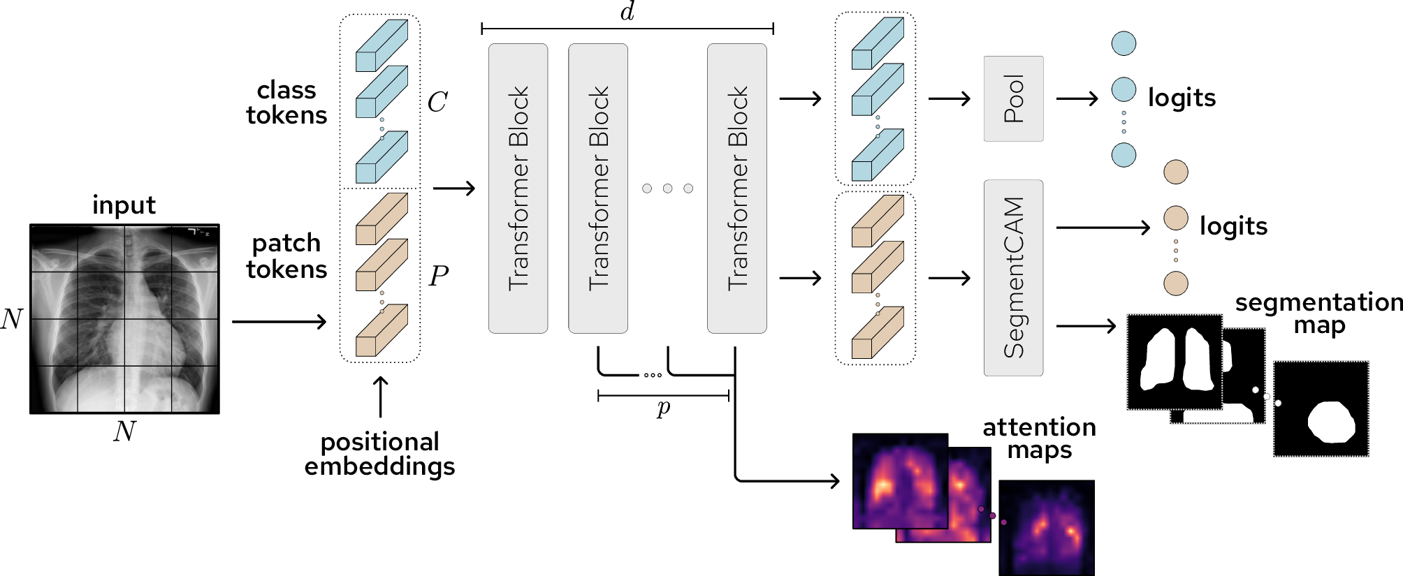
3.2 Weakly-supervised localization↩︎
This section describes our approach to weakly-supervised localization of pathologies in chest X-rays using a vision transformer with multiple class tokens. We first extract class-specific attention maps from the transformer’s self-attention matrix, averaged across the final model layers. These are then fused with foreground masks during inference to produce precise localization heatmaps, constrained to relevant anatomical regions via background suppression.
3.2.1 Class-specific attention maps↩︎
A vision transformer with multiple class tokens, where each class token corresponds to a single class, results in class-specific attention maps \(\boldsymbol{A}\). The class-to-patch sub-matrix in the transformer self-attention, as shown in 2, is extracted to obtain these attention maps.
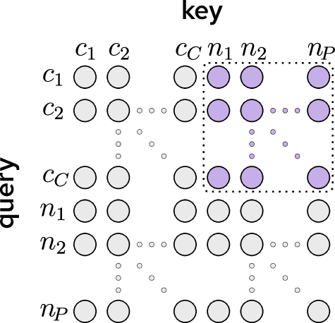
Using the class-to-patch attention, the class-specific attention maps are computed by averaging across the final \(p\) transformer layers: \[\boldsymbol{A}^{\left(i,j,c\right)} = \frac{1}{p} \sum_{l}^{p} \boldsymbol{A}_{l}^{\left(i,j,c\right)} , \quad \boldsymbol{A}_{l} \in {\left( 0,1 \right)}^{H \times W \times C}\] where \(\boldsymbol{A}^{\left(i,j,c\right)}\): class-specific attention map of class \(c\) at index \(\left(i,j\right)\), \(\boldsymbol{A}_{l}^{\left(i,j,c\right)}\): class-specific attention map of class \(c\) at layer \(l\) and index \(\left(i,j\right)\), \(l\): layer index, \(i\): image height index, \(j\): image width index, and \(c\): class index.
3.2.2 Heatmaps↩︎
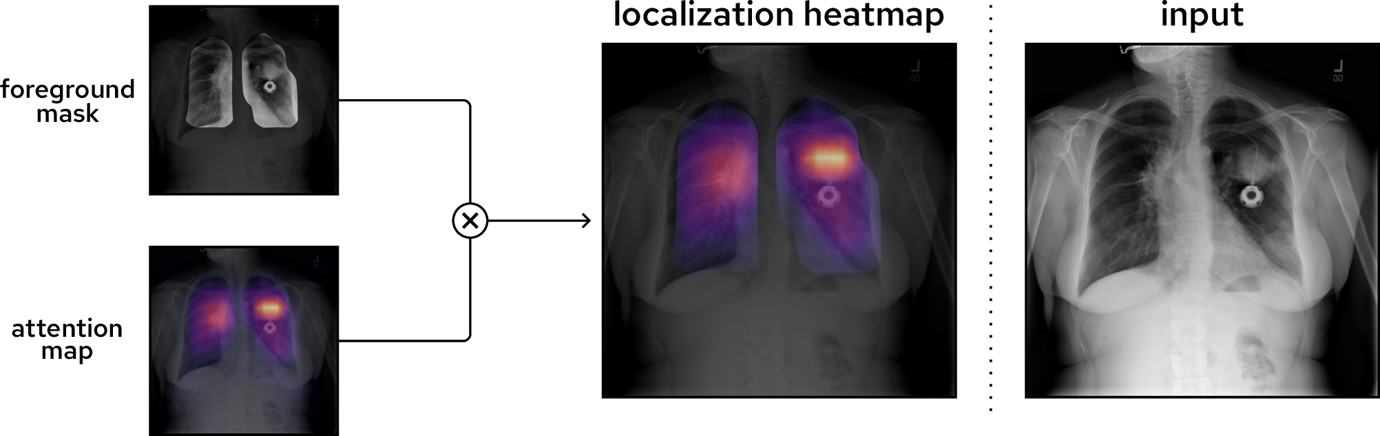
During inference, localization heatmaps \(\boldsymbol{\mathit{\Xi}} \in \left( 0,1 \right)^{H \times W \times C}\) are produced by fusing each class-specific foreground mask and attention map using element-wise multiplication: \[\boldsymbol{\mathit{\Xi}}^{\left(i,j,c\right)} = \boldsymbol{A}^{\left(i,j,c\right)} \thinspace \boldsymbol{S}_{\negthinspace f}^{\,\left(i,j,c\right)}\] where \(\boldsymbol{\mathit{\Xi}}^{\left(i,j,c\right)}\): localization heatmap of class \(c\) at index \(\left(i,j\right)\), and \(\boldsymbol{S}_{\negthinspace f}^{\,\left(i,j,c\right)}\): foreground mask of class \(c\) at index \(\left(i,j\right)\).
Each foreground mask ensures that the localization heatmap is constrained to class-specific foreground regions. Additionally, the background suppression methodology (3.5.2) enforces a prior over potential locations of classes. The result is a highly precise localization of chest X-ray pathologies, which is seen in 3 with regards to the large mass in the upper-middle region of the left lung.
3.3 Class tokens↩︎
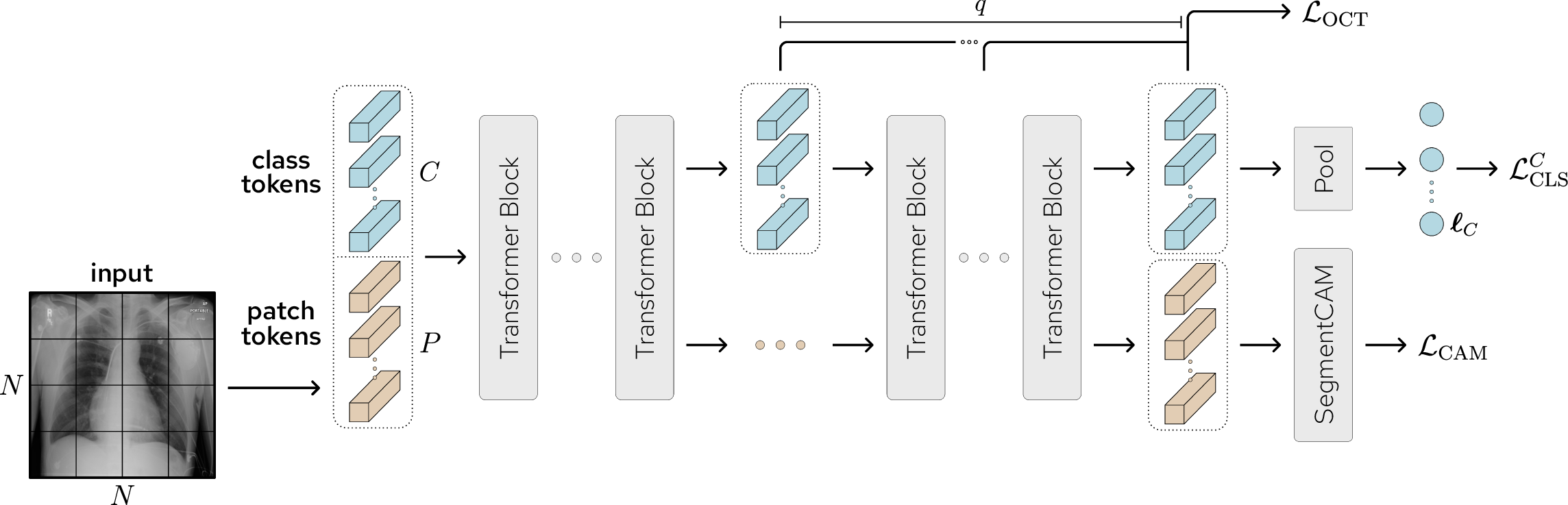
This section details the mechanisms involving class tokens in the CLARiTy model, including classification losses, orthogonality regularization, and attention pooling. A further illustration of the proposed model is shown in 4. The class token logits \(\boldsymbol{\ell}_C\) are used in the classification loss \(\mathcal{L}^{C}_{\mathrm{CLS}}\). The SegmentCAM module produces a combined CAM loss \(\mathcal{L}_{\mathrm{CAM}}\). Finally, an orthogonal class token loss \(\mathcal{L}_{\mathrm{OCT}}\) is applied to the class tokens produced from the final \(q\) transformer blocks.
3.3.1 Classification↩︎
The classification loss is the weighted binary cross-entropy (WBCE): \[\begin{align} \mathcal{L}_{\mathrm{CLS}}(\boldsymbol{\ell}, \boldsymbol{y}) = - \sum_{c=1}^C \thinspace\Bigl[ & w_{ P}\boldsymbol{y}^{\left(c\right)} \ln \sigma\left(\boldsymbol{\ell}^{\left(c\right)}\right) + \\ & w_{ N} \left(1 - \boldsymbol{y}^{\left(c\right)}\right) \ln \left(1 - \sigma\left(\boldsymbol{\ell}^{\left(c\right)}\right)\right) \Bigr] \end{align} \label{eqn95L95CLS}\tag{1}\] where \(\mathcal{L}_{\mathrm{CLS}}\): classification loss, \(\boldsymbol{\ell} \in \mathbb{R}^{C}\): predicted logits, \(\boldsymbol{y} \in \{0,1\}^{C}\): ground-truth binary labels, \(w_{ P}\): positive-label weight, \(w_{ N}\): negative-label weight, \(\boldsymbol{y}^{\left(c\right)}\): label at index \(c\), and \(\boldsymbol{\ell}^{\left(c\right)}\): predicted logit at index \(c\).
Sigmoid activation is applied to logits for multi-label probabilities: \[\begin{align} \sigma \left( x\right) = \frac{1}{1 + \exp\left(-x\right)} , \quad x \in \mathbb{R} . \label{eqn95sigmoid} \end{align}\tag{2}\]
Weights \(w_{ P}\) and \(w_{ N}\) are applied to positive and negative labels respectively, which dynamically handle class imbalances. Weights are calculated over all classes in a single batch: \[\begin{align} w_{ P} = \frac{\lvert P \rvert + \lvert N \rvert}{\lvert P \rvert} \nonumber \\ w_{ N} = \frac{\lvert P \rvert + \lvert N \rvert}{\lvert N \rvert} \nonumber \end{align}\] where \(\lvert P \rvert\): number of positive labels in the batch, and \(\lvert N \rvert\): number of negative labels in the batch.
Using 1 , the classification loss applied to the class token logits is \[\begin{align} \mathcal{L}_{\mathrm{CLS}}^{C} = \mathcal{L}_{\mathrm{CLS}}(\boldsymbol{\ell}_{C}, \boldsymbol{y}) \label{eqn95L95CLS94C} \end{align}\tag{3}\] where \(\mathcal{L}_{\mathrm{CLS}}^{C}\): class token classification loss.
3.3.2 Class token orthogonality↩︎
A regularization loss is applied to the class tokens, which drives them to mutual orthogonality. This affects the class-to-patch attention by causing each class token to attend to different image regions. To regularize for orthogonality, the class-to-class cosine similarity for each layer of class tokens is computed using \[\boldsymbol{\mathit{\Theta}}_l = \frac{\boldsymbol{T}_l \boldsymbol{T}_l^\top}{\|\boldsymbol{T}_l\|_{2,\mathrm{row}} \|\boldsymbol{T}_l\|_{2, \mathrm{row}}^\top}, \quad \boldsymbol{T}_l \in \mathbb{R}^{C \times D}, \quad \boldsymbol{\mathit{\Theta}}_l \in {\left[ -1,1 \right]}^{C \times C} \label{eqn:theta-cosine-similarity}\tag{4}\] where \(\boldsymbol{\mathit{\Theta}}_l\): cosine similarity matrix of layer \(l\), \(\boldsymbol{T}_l\): class token matrix of layer \(l\), and \(\|\cdot\|_{2, \mathrm{row}}\): row-wise norm.
The diagonal (self-similarity) is masked with \[\boldsymbol{M} = \mathbf{1} - \mathbf{I}_C, \quad \boldsymbol{M} \in \{0,1\}^{C \times C} \nonumber\] where \(\boldsymbol{M}\): mask matrix, \(\mathbf{1}\): ones matrix, \(\mathbf{I}_C\): identity matrix.
The orthogonal class token (OCT) loss is only applied to positive classes, and applied to all layers \(q\): \[\begin{align} \mathcal{L}_{\mathrm{OCT}} = &\frac{1}{\left( C-1 \right) \left[ q \sum_{c=1}^C \boldsymbol{y}^{\left(c\right)} + \varepsilon \right]} \sum_{l=1}^q \sum_{c=1}^C \sum_{k=1}^C \\ &{\boldsymbol{M}}^{\left(c,k\right)} \left( \boldsymbol{\mathit{\Theta}}^{\left(l,c,k\right)} - \theta \right)^2 \boldsymbol{y}^{\left(c\right)} \label{eqn95L95OCT} \end{align}\tag{5}\] where \(\mathcal{L}_{\mathrm{OCT}}\): orthogonal class token loss, \(k\): class index, \({\boldsymbol{M}}^{\left(c,k\right)}\): mask value at index \(\left(c,k\right)\), \(\boldsymbol{\mathit{\Theta}}^{\left(l,c,k\right)}\): cosine similarity of layer \(l\) at index \(\left(c,k\right)\), \(\theta\): target cosine similarity (\(\theta = 0\)), and \(\varepsilon\): small value to ensure numerical stability (\(\varepsilon = 1\times 10^{-8}\)).
3.3.3 Attention pooling↩︎
Typically, global average pooling (GAP) is applied to class tokens to obtain classification logits [60]. Attention pooling, however, complements the orthogonal class token loss by permitting each dimension of the embedding \(D\) to correspond to different classes. 5 shows the attention pooling module, which contains learned attention weights (invariant to the input image) applied to all class tokens. The \(\mathrm{softmax}\) function is applied row-wise to linear weights: \[\mathrm{softmax} \left( \boldsymbol{X} \right) ^ {\left(c,\varphi\right)} = \frac{ \exp \left(\boldsymbol{X}^{\left(c,\varphi\right)} \right) }{ \sum_{\psi=1}^{D} \exp \left(\boldsymbol{X}^{\left(c,\psi\right)} \right) } , \quad \boldsymbol{X} \in \mathbb{R}^{C \times D}\] where \(\mathrm{softmax} \left( \boldsymbol{X} \right) ^ {\left(c,\varphi\right)}\): attention weight at index \(\left(c,\varphi\right)\), \(\boldsymbol{X}\): learned linear weights, \(\boldsymbol{X}^{\left(c,\varphi\right)}\) and \(\boldsymbol{X}^{\left(c,\psi\right)}\): linear weight at index \(\left(c,\varphi\right)\) and \(\left(c,\psi\right)\) respectively, \(\varphi\) and \(\psi\): embedding indices.
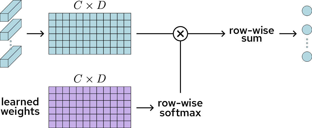
Now we can pool each class token into a single logit using: \[\mathrm{AttnPool} \left( \boldsymbol{T}, \boldsymbol{X} \right) ^ {\left(c\right)} = \sum_{\varphi=1}^{D} \boldsymbol{T}^{\left(c,\varphi\right)} \, \mathrm{softmax} \left( \boldsymbol{X} \right) ^ {\left(c,\varphi\right)} = \boldsymbol{\ell}_{C}^{\left(c\right)}\] where \(\boldsymbol{T} \in \mathbb{R}^{C \times D}\): output class token matrix, \(\boldsymbol{T}^{\left(c,\varphi\right)}\): class token matrix at index \(\left(c,\varphi\right)\), \(\mathrm{AttnPool} \left( \boldsymbol{T}, \boldsymbol{X} \right) ^ {\left(c\right)}\): attention pooling result of class token \(c\), and \(\boldsymbol{\ell}_{C}^{\left(c\right)}\): predicted logit of class token \(c\).
3.4 SegmentCAM feature and heatmap extraction↩︎
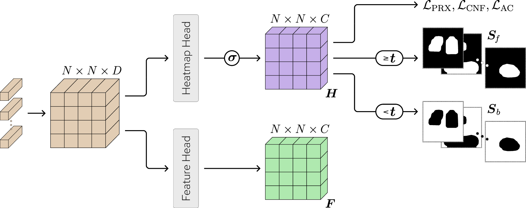
This section outlines the first stage of our proposed SegmentCAM module (6), inspired by [61], which involves feature and heatmap extraction from reshaped patch tokens, followed by the application of three specialized loss functions: mask proximity to penalize distant activations, mask confinement to restrict background intensity, and area constraint to limit foreground size. It also covers resampling of heatmaps and segmentation maps for computational efficiency.
In this first stage, the output patch tokens are reshaped to an \(N \times N \times D\) tensor and passed through two convolutional heads. The heads reduce the number of channels from \(D\) to the number of classes \(C\). Each head is a fused inverse bottleneck with an expansion ratio of 2 (8). The heatmap head uses sigmoid activation (2 ) to produce a heatmap tensor \(\boldsymbol{H} \in \left(0,1\right)^{N \times N \times C}\). A fixed threshold \(t \in \left(0,1\right)\) is applied to \(\boldsymbol{H}\), which produces the foreground and background segmentation maps \(\boldsymbol{S}_{\negthinspace f}\) and \(\boldsymbol{S}_{b} \in \{0,1\}^{N \times N \times C}\), respectively. The feature head produces the feature tensor \(\boldsymbol{F} \in \mathbb{R}^{N \times N \times C}\), which is used in the second stage. Finally, three loss functions are applied to \(\boldsymbol{H}\): the mask proximity loss \(\mathcal{L}_{\mathrm{PRX}}\), the mask confinement loss \(\mathcal{L}_{\mathrm{CNF}}\), and the area constraint loss \(\mathcal{L}_{\mathrm{AC}}\).
3.4.1 Mask proximity↩︎
The mask proximity loss penalizes the model for producing heatmap intensity far from the foreground. Heatmap intensity within the foreground has a loss value of zero. The Euclidean distance transform is applied to the negation of the ground-truth segmentation map (\(\neg \boldsymbol{S}\)), which calculates the distance from each background pixel to its nearest foreground pixel: \[\begin{align} \boldsymbol{D} &= \mathrm{EDT}\left(\neg \boldsymbol{S}\right), \quad \boldsymbol{S} \in \{0,1\}^{H \times W \times C}, \boldsymbol{D} \in \mathbb{R}_{\geq 0}^{H \times W \times C} \nonumber \end{align}\] where \(\boldsymbol{D}\): distance tensor, \(\mathrm{EDT}\left(\cdot\right)\): Euclidean distance transform function, and \(\boldsymbol{S}\): ground-truth segmentation map.
The distance tensor is then element-wise multiplied by the heatmap tensor and the similarity weight vector \(\boldsymbol{w} \in \mathbb{R}_{\geq 1}^{C}\): \[\mathcal{L}_{\mathrm{PRX}} = \frac{8}{HWC \left(H+W\right)} \sum_{i=1}^H \sum_{j=1}^W \sum_{c=1}^C \boldsymbol{H}^{\left(i,j,c\right)} \thinspace \boldsymbol{D}^{\left(i,j,c\right)} \thinspace \boldsymbol{w}^{\left(c\right)} \label{eqn95L95PROX}\tag{6}\] where \(\mathcal{L}_{\mathrm{PRX}}\): mask proximity loss, \(\boldsymbol{H}^{\left(i,j,c\right)}\): heatmap intensity at index (\(i,j,c\)), \(\boldsymbol{D}^{\left(i,j,c\right)}\): euclidean distance at index (\(i,j,c\)), and \(\boldsymbol{w}^{\left(c\right)}\): similarity weight of class \(c\).
Since many chest X-ray pathologies exist in the same region (such as the lung lobes), \(\boldsymbol{w}\) is used to increase learning pressure on less-commonly masked regions. After vectorizing each mask in the ground-truth segmentation map, the cosine similarity is computed between each class’ mask: \[\begin{align} \boldsymbol{U} &= \mathrm{vec}\left(\boldsymbol{S}\right), \quad \boldsymbol{U} \in \{ 0,1 \}^{\left(H W\right) \times C} \nonumber \\ \boldsymbol{V} &= \frac{\boldsymbol{U}^\top \boldsymbol{U}}{\|\boldsymbol{U}\|_{2, \mathrm{row}}^\top \|\boldsymbol{U}\|_{2, \mathrm{row}}}, \quad \boldsymbol{V} \in {\left[-1,1\right]}^{C \times C} \nonumber \end{align}\] where \(\boldsymbol{U}\): vectorized segmentation map, and \(\boldsymbol{V}\): cosine similarity matrix.
The average inter-class similarity \(\boldsymbol{\mu} \in {\left[-1,1\right]}^{C}\) is found by averaging across each row of \(\boldsymbol{V}\) (ignoring the diagonal). This represents the average similarity between each class \(c\) and all other classes \(k\) (\(k \neq c\)): \[\boldsymbol{\mu}^{\left(c\right)} = \frac{1}{C - 1} \sum_{\substack{k=1 \\ k \neq c}}^C \boldsymbol{V}^{\left(c,k\right)} \nonumber\] where \(\boldsymbol{\mu}^{\left(c\right)}\): average inter-class similarity of class \(c\), and \(\boldsymbol{V}^{\left(c,k\right)}\): cosine similarity at index (\(c,k\)).
To transform the vector \(\boldsymbol{\mu}\) from a similarity metric to weights, the range of values is inverted and the minimum value is set to 1: \[\boldsymbol{w} = 2 - \boldsymbol{\mu} - \min_{c} \left(\boldsymbol{\mu}^{\left(c\right)} \right) \label{eqn95w}\tag{7}\] where \(\boldsymbol{w}\): segmentation similarity weights.
When the mask of class \(c\) is very similar to all other masks of classes \(k\), then its weight value will be near 1. For such a value, the segmentation loss for \(c\) is unaffected. If, however, the mask of \(c\) is highly dissimilar to all masks of \(k\), then there is increased loss applied to \(c\) as the weight value is greater than 1.
3.4.2 Mask confinement↩︎
The mask confinement loss penalizes any heatmap intensity within the background. The model then learns to predict foreground that is confined within the ground-truth masked regions. It is defined as the ratio of heatmap intensity within the background to total heatmap intensity: \[\begin{align} \mathcal{L}_{\mathrm{CNF}} = \frac{1}{H WC} \sum_{i=1}^H \sum_{j=1}^W \sum_{c=1}^C \frac{ \boldsymbol{H}^{\left(i,j,c\right)} \thinspace {\neg{\boldsymbol{S}}}^{\left(i,j,c\right)} \thinspace \boldsymbol{w}^{\left(c\right)} }{ \boldsymbol{H}^{\left(i,j,c\right)}} \label{eqn95L95CONF} \end{align}\tag{8}\] where \(\mathcal{L}_{\mathrm{CNF}}\): mask confinement loss, and \(\boldsymbol{S}^{\left(i,j,c\right)}\): ground-truth segmentation map at index \(\left(i,j,c\right)\).
3.4.3 Foreground area↩︎
The area constraint loss reduces the total heatmap intensity, which limits the foreground area: \[\begin{align} \mathcal{L}_{\mathrm{AC}} = \frac{1}{H WC} \sum_{i=1}^H \sum_{j=1}^W \sum_{c=1}^C \boldsymbol{H}^{\left(i,j,c\right)} \label{eqn95L95AC} \end{align}\tag{9}\] where \(\mathcal{L}_{\mathrm{AC}}\): area constraint loss.
3.4.4 Heatmap and segmentation map resampling↩︎
The heatmap tensor \(\boldsymbol{H}\) and ground-truth segmentation map \(\boldsymbol{S}\) are both resampled to \(64 \times 64\) when computing the losses \(\mathcal{L}_{\mathrm{PRX}}\), \(\mathcal{L}_{\mathrm{CNF}}\), and \(\mathcal{L}_{\mathrm{AC}}\). \(\boldsymbol{S}\) is downsampled to reduce computational cost, while \(\boldsymbol{H}\) is upsampled to ensure it retains more spatial detail. Resampling is done via bilinear interpolation.
3.5 SegmentCAM background activation suppression↩︎
This section details the second stage of the SegmentCAM module (7), where background activation suppression is achieved by creating tensors with selectively suppressed features, processing them through a convolutional classification head to derive specialized logits, and applying targeted classification and suppression losses to prioritize foreground-relevant information.
In this second stage, foreground suppression is applied to the feature tensor \(\boldsymbol{F}\) by fusing it with the background segmentation map \(\boldsymbol{S}_{b}\). Both the suppressed and unsuppressed feature tensors are passed through the same convolutional classification head. This head is comprised of three fused inverse bottleneck blocks, each with an expansion ratio of 2 (8). After the classification head, the unsuppressed feature tensor is fused with \(\boldsymbol{S}_{\negthinspace f}\) in a separate branch. Global average pooling is then applied to all final feature tensors, producing classification logits. The foreground logits \(\boldsymbol{\ell}_{\negthinspace f}\) contain only foreground information, while the background logits \(\boldsymbol{\ell}_{b}\) contain only background information. The patch token logits \(\boldsymbol{\ell}_{ P}\) contain information from the unmasked features. The classification head learns to only classify foreground-specific features using three loss functions. The foreground classification loss \(\mathcal{L}^{f}_{\mathrm{CLS}}\) is applied to \(\boldsymbol{\ell}_{\negthinspace f}\), the patch token classification loss \(\mathcal{L}^{P}_{\mathrm{CLS}}\) is applied to \(\boldsymbol{\ell}_{ P}\), and the background activation suppression loss \(\mathcal{L}_{\mathrm{BAS}}\) is applied to both \(\boldsymbol{\ell}_{ P}\) and \(\boldsymbol{\ell}_{b}\).

3.5.1 Classification↩︎
The foreground and patch token losses both use the weighted binary cross-entropy loss function (1 ). These losses guide the SegmentCAM module to only identify class-relevant information within foreground regions: \[\begin{align} \mathcal{L}_{\mathrm{CLS}}^{f} &= \mathcal{L}_{\mathrm{CLS}}(\boldsymbol{\ell}_{\negthinspace f}, \boldsymbol{y}) \tag{10} \\ \mathcal{L}_{\mathrm{CLS}}^{P} &= \mathcal{L}_{\mathrm{CLS}}(\boldsymbol{\ell}_{ P}, \boldsymbol{y}) \tag{11} \end{align}\] where \(\mathcal{L}_{\mathrm{CLS}}^{f}\): foreground classification loss, and \(\mathcal{L}_{\mathrm{CLS}}^{P}\): patch token classification loss.
3.5.2 Background activation suppression↩︎
The background activation suppression loss is designed to reduce the amount of information retained in the background logits relative to the patch token logits. Commonly, \(\mathrm{ReLU}\) activation is applied to these logits to obtain non-zero activations [61]. To prevent numerical instability, \(\mathrm{softplus}\) activation is used instead: \[\mathrm{softplus}\left(x\right) = \ln \left( 1 + \exp \left(x\right) \right).\]
Applying only to positive classes, the background activation suppression loss is \[\begin{align} \mathcal{L}_{\mathrm{BAS}} = \frac{1}{\max\left(\sum_{c=1}^C \boldsymbol{y}^{\left(c\right)}, 1\right)} \sum_{c=1}^C \boldsymbol{y}^{\left(c\right)} \frac{ \mathrm{softplus}\left( \boldsymbol{\ell}_{b}^{\left(c\right)} \right) }{ \mathrm{softplus}\left( \boldsymbol{\ell}_{ P}^{\left(c\right)} \right) + \varepsilon} \end{align}\] where \(\mathcal{L}_{\mathrm{BAS}}\): background activation suppression loss, \(\boldsymbol{\ell}_{b}^{\left(c\right)}\): background logit of class \(c\), and \(\boldsymbol{\ell}_{ P}^{\left(c\right)}\): patch token logit of class \(c\).
![Figure 8: Fused inverse bottleneck block, as used in [62]. An input tensor of shape H \times W \times K_1 is passed through a 3 \times 3 convolution with an expansion ratio of r \in \mathbb{R}_{> 1}. This increases the number of channels to rK_1. Thereafter, batch normalization and \mathrm{SiLU} activation is applied. Finally, a 1 \times 1 convolution with batch normalization reduces the number of channels to K_2. If K_1=K_2, then a residual connection is added to the output.](/article/2512.16700/figure-8_fused-inverse-bottleneck.png "fig:")
3.6 Combined loss↩︎
All component loss functions are combined into a single loss using scalar weights \(\alpha_C\), \(\alpha_{ P}\), \(\alpha_{\negthinspace f}\), \(\beta_1\), \(\beta_2\), \(\gamma_1\), \(\gamma_2\) and \(\delta\): \[\mathcal{L} = \alpha_C \mathcal{L}_{\mathrm{CLS}}^{C} + \mathcal{L}_{\mathrm{CAM}} + \delta \mathcal{L}_{\mathrm{OCT}}\] where \(\mathcal{L}\): combined loss, and the CAM loss \(\left ( \mathcal{L}_{\mathrm{CAM}} \right )\) is defined as: \[\begin{align} \mathcal{L}_{\mathrm{CAM}} = \alpha_{ P} \mathcal{L}_{\mathrm{CLS}}^{P} +& \alpha_{\negthinspace f} \mathcal{L}_{\mathrm{CLS}}^{f} + \beta_1 \mathcal{L}_{\mathrm{BAS}} + \beta_2 \mathcal{L}_{\mathrm{AC}} + \\ & \gamma_1 \mathcal{L}_{\mathrm{PRX}} + \gamma_2 \mathcal{L}_{\mathrm{CNF}} . \end{align}\]
3.7 Dataset↩︎
The CLARiTy model was trained and evaluated on the official benchmark split of the NIH ChestX-ray14 dataset [21], which contains 112,120 frontal chest X-ray images of size \(1024 \times 1024\) from 30,805 patients. There are 14 co-occurring pathology classes, and the official train-test split is 80%–20%. The official training set was further split such that 70% of all images in the dataset were used for training, and 10% used for validation. All splits were done patient-wise, so that all images from the same patient reside in the same dataset split.
A subset of the test set has been annotated with bounding boxes, which denote radiologist-identified pathology regions. This subset includes 880 images and 984 bounding boxes. Bounding box annotations are only available for 8 of the 14 classes. These images were used to create a validation-test split of 50%–50% (patient-wise) for weakly-supervised localization.
3.8 Metrics↩︎
This section outlines the metrics used to evaluate model performance in classification and weakly-supervised localization tasks. These include the area under the receiver operating characteristic curve (AUC) for classification; Intersection over Union (IoU) Accuracy and the Multi-Scale Localization Index (MSLI) for localization; and the Unified Detection Proficiency (UDP) for joint assessment. Finally, comparisons with reproduced models highlight dataset split impacts.
3.8.1 Classification↩︎
The AUC is the primary metric for evaluating the classification performance for each class. It is macro-averaged across all classes to obtain the Macro AUC.
3.8.2 Weakly-supervised localization↩︎
The IoU Accuracy is the primary metric for evaluating weakly-supervised localization performance. It is calculated using the IoU between pairs of predicted and ground-truth bounding boxes. If IoU\(>\)T(IoU) for a given bounding box pair, where \(\mathrm{T(IoU)} \in \left(0,1\right)\) is a threshold, then this is considered a successful localization. The proportion of ground-truth bounding boxes which are successfully localized is named the IoU Accuracy at the specified T(IoU). This metric can be macro-averaged across all classes to obtain the Macro IoU Accuracy at the specified T(IoU).
The Multi-Scale Localization Index (MSLI) is calculated by averaging the Macro IoU Accuracy over all T(IoU) in \(\{0.1, 0.25, 0.5, 0.75, 0.9\}\). The MSLI evaluates the localization performance over multiple degrees of spatial precision, from low to high IoU tolerance.
The weakly-supervised localization metrics for each class are calculated only on images where that class is correctly predicted by the model (i.e., the model assigns a positive label for that class).
3.8.3 Unified performance↩︎
Both the classification and weakly-supervised localization performance must be maximized jointly. Consequently, the Unified Detection Proficiency (UDP) is defined as the average between the Macro AUC and the MSLI. The UDP is optimized in ablation experiments.
3.8.4 Performance comparisons↩︎
As mentioned earlier, model performance differs significantly with dataset split (2). The highest reported Macro AUC for the NIH dataset in the literature is 0.853, achieved by the MLRFNet model [63]. We reproduced MLRFNet using the official NIH split, resulting in an absolute performance drop of 5.2% (¿tbl:tab:classification95comparison?). With our best efforts, while constrained by time, we also reproduced four other models—for which we could not verify that the published results used the official NIH split. We trained these using the official NIH split and tested only their classification performance. The absolute drop in Macro AUC for these models varied between 3.1%–6.3%. To enable comparison of model performance, all results are presented together irrespective of dataset split. However, when it is possible to verify that a model was (or was not) trained using the official NIH split, those models are grouped together.
3.9 Bounding boxes↩︎
To obtain bounding boxes from the localization heatmaps, thresholding is used. A class-specific threshold \(\boldsymbol{\xi}^{\left(c\right)} \in \left( 0,1 \right)\) is applied to a class’ localization heatmap \(\boldsymbol{\mathit{\Xi}}^{\left(c\right)}\) which produces connected regions. A single bounding box is created for each connected region. The optimal threshold \(\boldsymbol{\xi}^{\left(c\right)}\) is found by maximizing the MSLI on the localization-validation set.
3.10 Image resolution and augmentation↩︎
Models were trained at an image resolution of \(224 \times 224\) or \(512\times 512\) by downsampling the original \(1024 \times 1024\) images via the Lanczos method. Augmentations were applied to images during training, namely: random rotation, random cropping, random Poisson noise, and random brightness. All augmentations were generated using a pseudo-random generator, where the seed is unique for each combination of image and epoch number.
3.11 Ground-truth segmentation maps↩︎
The segmentation model provided in the TorchXrayVision library was used to produce the ground-truth segmentation maps [64], [65]. This model produces anatomical segmentations for chest X-ray images. A large language model (Grok) was prompted to list the possible anatomical regions (given by the segmentation model) wherein each NIH pathology could be located (1). The anatomical masks for each pathology are combined into a single region-of-interest mask. These region-of-interest masks are then combined into a segmentation map for each image. The anatomical regions predicted by Grok were validated by a diagnostic radiologist. The prompt given to Grok is shown in 7.
| Pathology | Anatomical Regions |
|---|---|
| Atelectasis | Left Lung, Right Lung |
| Cardiomegaly | Heart |
| Consolidation | Left Lung, Right Lung |
| Edema | Left Lung, Right Lung |
| Effusion | Left Lung, Right Lung |
| Emphysema | Left Lung, Right Lung |
| Fibrosis | Left Lung, Right Lung |
| Hernia | Facies Diaphragmatica, Mediastinum |
| Infiltration | Left Lung, Right Lung |
| Mass | Left Lung, Right Lung, Mediastinum |
| Nodule | Left Lung, Right Lung |
| Pleural Thickening | Left Lung, Right Lung |
| Pneumonia | Left Lung, Right Lung |
| Pneumothorax | Left Lung, Right Lung |
3.12 Distillation↩︎
The ConvNeXtV2-B is used as the teacher model for distillation. Using ImageNet pretrained weights, it was trained on the training set, and the best performing model was selected during training via the Macro AUC, by evaluating on the validation set after each epoch. The teacher was trained with image augmentations, using the weighted binary cross-entropy loss (1 ), for \(100\) epochs, with a batch size of \(1024\), learning rate of \(2.5 \times 10^{-5}\), using the AdamW optimizer, weight decay of \(0.05\), classifier head dropout rate of 0.1 and stochastic depth rate of 0.1. Finally, a cosine learning schedule was used with a warmup of 3 epochs. Two versions were trained at different resolutions: the ConvNeXtV2-B-224 at \(224\times 224\) and the ConvNeXtV2-B-512 at \(512\times 512\). Macro AUCs of \(0.833\) and \(0.850\) on the validation set were achieved by the ConvNeXtV2-B-224 and ConvNeXtV2-B-512, respectively.
To reduce the training time of the distillation, the TinyViT method was used [66]. This is an efficient method of distilling a teacher model into a vision transformer. The teacher probabilities are the learning target for classification, which are pre-computed and stored as logits ahead of distillation. Dense logits are stored, as opposed to the sparse logits used in the original TinyViT method. Teacher logits are pre-computed for each combination of epoch and augmented image.
3.13 Model specification↩︎
CLARiTy is built on the ViT-S-16 backbone, which has 12 layers, 6 self-attention heads per layer, embedding size of 384 and a patch size of 16. After an ablation study (4.5), the final 8 self-attention layers were used to create the class-specific attention maps, and the orthogonal class token loss was applied to the final 8 layers of class tokens.
The CLARiTy-S-16-224 configuration takes \(224\times 224\) images as input, resulting in a spatial resolution of \(14 \times 14\) for the output localization heatmaps. The heatmaps are upsampled to \(224 \times 224\) at inference using bilinear interpolation.
The CLARiTy-S-16-512 configuration takes \(512\times 512\) images as input, resulting in a spatial resolution of \(32 \times 32\) for the output localization heatmaps. The heatmaps are likewise upsampled to \(512 \times 512\) at inference using bilinear interpolation.
3.14 Training↩︎
Using DINO pretrained weights, the CLARiTy-S-16-224 was trained for \(200\) epochs, with a batch size of \(1024\), learning rate of \(1 \times 10^{-4}\) using the AdamW optimizer, weight decay of \(0.05\), attention pooling dropout rate of 0.1, stochastic depth rate of 0.1, MLP dropout rate of 0.1, and self-attention dropout rate of 0.1. Finally, a cosine learning schedule was used with a warmup of 5 epochs. The best performing model was selected during training via the UDP, by evaluating on the validation set after each epoch
The CLARiTy-S-16-512 was trained using the same methodology. However, instead of using DINO pretrained weights, it used the trained weights of the CLARiTy-S-16-224 and interpolated the positional embeddings for \(512\times 512\) images.
3.15 Hyperparameter tuning↩︎
Hyperparameter tuning used the CLARiTy-S-16-224 model to optimize loss weights \(\alpha_C\), \(\alpha_{ P}\), \(\alpha_{\negthinspace f}\), \(\beta_1\), \(\beta_2\), \(\gamma_1\), \(\gamma_2\) and \(\delta\). We employed a sampler with Optuna’s Tree-structured Parzen Estimator (TPE) algorithm [67], [68], with 20 trials, 10 startup trials, and 100 candidate samples per trial. Each scalar weight was searched over \(\left[ 0,5 \right]\). The optimization objective maximized classification and weakly-supervised localization performance on the validation set using the UDP. The optimal loss weights are given in 2.
| Loss Weight | Value |
|---|---|
| \(\alpha_C\) | 2.2674 |
| \(\alpha_{\hspace{-0.08em} P}\) | 2.4678 |
| \(\alpha_{\negthinspace f}\) | 3.9670 |
| \(\beta_1\) | 0.4377 |
| \(\beta_2\) | 1.4000 |
| \(\gamma_1\) | 0.0898 |
| \(\gamma_2\) | 2.1624 |
| \(\delta\) | 2.6375 |
4 Results↩︎
This section presents the experimental results of the proposed CLARiTy model, including quantitative comparisons on classification and weakly-supervised localization tasks, qualitative visualizations, resource requirements, and ablation studies. Models performing both classification and weakly-supervised localization are compared in ¿tbl:tab:combined95performance?. Detailed comparisons of classification and localization performance are provided in ¿tbl:tab:classification95comparison? ¿tbl:tab:localization95comparison?, respectively. Ablation results are given in ¿tbl:tab:ablation95comparison?.
@ l c c ccccblccccrmccccccc *5c & & & &
& & & & 0.1 & 0.2 & 0.3 & 0.4 & 0.5
RGT1 & 224 & 70% & 0.839† & 0.591 & 0.424 & 0.281 & 0.173 & 0.090
ThoraX-PriorNet-2242 & 224 & 70% & 0.844 & 0.666 & 0.509 & 0.398 & 0.296 & 0.201
ThoraX-PriorNet-5122 & 512 & 70% & 0.847 & 0.803 & 0.626 & 0.488 & 0.334 & 0.217
[21] & 1024 & 70% & 0.745 & 0.568 & 0.373 & 0.221 & 0.116 & 0.062
[45] & 512 & 80% & 0.829 & 0.639 & 0.527 & 0.397 & 0.314 & 0.243
PCAN3 & 512 & 80% & 0.830 & 0.778 & 0.574 & 0.364 & 0.207 & 0.103
CLARiTy-S-16-224 & 224 & 70% & 0.799 & 0.773 & 0.614 & 0.502 & 0.394 & 0.303
CLARiTy-S-16-512 & 512 & 70% & 0.818 & 0.814 & 0.688 & 0.588 & 0.470 & 0.318
>
X *15S[table-format=1.3]
&
& Atel. & Card. & Cons. & Edem. & Effu. & Emph. & Fibr. & Hern. & Infi. & Mass &
Nodu. & Pleu. & Pn. 1 & Pn. 2 & Mean
[69] & 0.772 & 0.904 & 0.788 & 0.882 & 0.859 & 0.829 & 0.767 & 0.914 & 0.695 & 0.792 & 0.717 &
0.765 & 0.713 & 0.841 & 0.798
[49] & 0.800 & 0.870 & 0.800 & 0.880 & 0.870 & 0.910 & 0.780 & 0.770 & 0.700 & 0.830 & 0.750 & 0.790
& 0.670 & 0.870 & 0.806
[70] & 0.795 & 0.887 & 0.786 & 0.892 & 0.875 & 0.875 & 0.756 & 0.836 & 0.703 & 0.835 & 0.716 & 0.774
& 0.742 & 0.863 & 0.810
[70] & 0.726 & 0.865 & 0.717 & 0.812 & 0.810 & 0.740 & 0.748 & 0.803 & 0.682 & 0.773 & 0.686 & 0.730 &
0.660 & 0.796 & 0.753
RGT1 & 0.800† & 0.920† & & & 0.780† & & & & 0.860† & 0.880† & 0.880† & & 0.790† & 0.810† &
0.839†
MLRFNet2 & 0.833 & 0.915 & 0.826 & 0.905 & 0.884 & 0.941 & 0.821 & 0.963 & 0.717 & 0.858 & 0.799 & 0.810 &
0.760 & 0.900 & 0.853
MLRFNet & 0.756 & 0.888 & 0.742 & 0.840 & 0.821 & 0.894 & 0.816 & 0.910 & 0.684 & 0.808 & 0.735 & 0.760 & 0.711 & 0.850 & 0.801
[71] & 0.817 & 0.911 & 0.815 & 0.908 & 0.879 & 0.935 & 0.824 & 0.890 & 0.716 &
0.853 & 0.771 & 0.812 & 0.769 & 0.898 & 0.843
[71] & 0.766 & 0.863 & 0.736 & 0.846 & 0.830 & 0.926 & 0.818 & 0.846 & 0.699 & 0.794 & 0.740 & 0.776
& 0.725 & 0.873 & 0.803
ThoraX-PriorNet-2243 & 0.826 & 0.906 & 0.819 & 0.910 & 0.884 & 0.924 & 0.818 & 0.919 & 0.723 & 0.864 & 0.780 & 0.800 & 0.770 &
0.880 & 0.844
ThoraX-PriorNet-5123 & 0.827 & 0.902 & 0.812 & 0.908 & 0.884 & 0.927 & 0.826 & 0.905 & 0.723 & 0.867 & 0.807 & 0.813 & 0.764 & 0.890 &
0.847
[72] & 0.803 & 0.906 & 0.776 & 0.874 & 0.851 & 0.940 & 0.842 & 0.915 & 0.735 & 0.858 &
0.790 & 0.789 & 0.746 & 0.887 & 0.837
[72] & 0.768 & 0.895 & 0.744 & 0.839 & 0.827 & 0.902 & 0.814 & 0.898 & 0.700 & 0.816 & 0.753 &
0.768 & 0.709 & 0.855 & 0.806
HydraViT4 & 0.810 & 0.904 & 0.822 & 0.882 & 0.878 & 0.908 & 0.845 & 0.908 & 0.755 & 0.840 & 0.800 & 0.830 & 0.758 & 0.876
& 0.841
HydraViT & 0.732 & 0.876 & 0.720 & 0.822 & 0.804 & 0.889 & 0.795 & 0.844 & 0.695 & 0.776 & 0.690 & 0.736 & 0.679 & 0.837 & 0.778
[21] & 0.700 & 0.810 & 0.703 & 0.805 & 0.759 & 0.833 & 0.786 & 0.872 & 0.661 & 0.693 & 0.669 &
0.684 & 0.658 & 0.799 & 0.745
[44] & 0.733 & 0.856 & 0.711 & 0.806 & 0.806 & 0.842 & 0.743 & 0.775 & 0.673 & 0.777 & 0.718 & 0.724
& 0.684 & 0.805 & 0.761
[27] & 0.756 & 0.887 & 0.728 & 0.848 & 0.819 & 0.908 & 0.818 & 0.875 & 0.689 & 0.814 & 0.755 & 0.765 &
0.729 & 0.850 & 0.803
[33] & 0.767 & 0.883 & 0.745 & 0.835 & 0.828 & 0.895 & 0.818 & 0.896 & 0.709 & 0.821 & 0.758 & 0.761
& 0.731 & 0.846 & 0.807
SDFN5 & 0.781 & 0.885 & 0.743 & 0.842 & 0.832 & 0.921 & 0.835 & 0.911 & 0.700 & 0.815 & 0.765 & 0.791 & 0.719 & 0.866 & 0.815
[73] & 0.777 & 0.894 & 0.750 & 0.846 & 0.829 & 0.908 & 0.827 & 0.934 & 0.696 & 0.838 & 0.771 & 0.779 &
0.722 & 0.862 & 0.817
Thorax-Net6 & 0.751 & 0.871 & 0.742 & 0.835 & 0.818 & 0.843 & 0.804 & 0.902 & 0.682 & 0.799 & 0.715 & 0.746 & 0.694 & 0.825 & 0.788
CRAL7 & 0.781 & 0.880 & 0.754 & 0.850 & 0.829 & 0.908 & 0.830 & 0.917 & 0.702 & 0.834 & 0.773 & 0.778 & 0.729 & 0.857 & 0.816
[74] & 0.786 & 0.893 & 0.751 & 0.850 & 0.832 & 0.944 & 0.834 & 0.929 & 0.699 & 0.840 &
0.800 & 0.795 & 0.739 & 0.876 & 0.826
[41] & 0.785 & 0.899 & 0.763 & 0.850 & 0.835 & 0.924 & 0.831 & 0.922 & 0.699 & 0.838 & 0.775 & 0.776 &
0.738 & 0.871 & 0.822
[40] & 0.770 & 0.870 & 0.740 & 0.840 & 0.830 & 0.940 & 0.830 & 0.910 & 0.710 & 0.830 & 0.790 & 0.790
& 0.720 & 0.880 & 0.819
SwinCheX8 & 0.781 & 0.875 & 0.748 & 0.848 & 0.824 & 0.914 & 0.826 & 0.855 & 0.701 & 0.822 & 0.780 & 0.778 & 0.713 & 0.871 & 0.810
[45] & 0.797 & 0.872 & 0.779 & 0.858 & 0.852 & 0.935 & 0.825 & 0.907 & 0.711 & 0.843 & 0.795 & 0.800
& 0.742 & 0.894 & 0.829
PCAN9 & 0.791 & 0.887 & 0.759 & 0.854 & 0.841 & 0.944 & 0.819 & 0.928 & 0.711 & 0.839 & 0.809 & 0.806 & 0.746 & 0.881 & 0.830
ConvNeXtV2-B-224 & 0.763 & 0.894 & 0.750 & 0.853 & 0.827 & 0.908 & 0.805 & 0.901 & 0.689 & 0.814 & 0.751 & 0.773 & 0.718 & 0.857 & 0.807
ConvNeXtV2-B-512 & 0.785 & 0.900 & 0.755 & 0.851 & 0.833 & 0.940 & 0.842 & 0.919 & 0.701 & 0.839 & 0.797 & 0.780 & 0.737 & 0.877 & 0.825
CLARiTy-S-16-224 & 0.760 & 0.895 & 0.755 & 0.844 & 0.826 & 0.887 & 0.817 & 0.839 & 0.692 & 0.808 & 0.736 & 0.765 & 0.707 & 0.854 & 0.799
CLARiTy-S-16-512 & 0.784 & 0.899 & 0.759 & 0.855 & 0.837 & 0.939 & 0.831 & 0.854 & 0.700 & 0.827 & 0.783 & 0.779 & 0.735 & 0.874 & 0.818
Pathologies are: Atelectasis, Cardiomegaly, Consolidation, Edema, Effusion, Emphysema, Fibrosis, Hernia, Infiltration, Mass, Nodule, Pleural Thickening, Pneumonia, and Pneumothorax.
† Classification performance evaluated on 8 pathologies: Atelectasis, Cardiomegaly, Effusion, Infiltration, Mass, Nodule, Pneumonia, and Pneumothorax.
We could not verify that published model results used the official NIH dataset split.
1 [57] 2 [63] 3 [35] 4 [54] 5 [30] 6 [37] 7 [75] 8 [76] 9 [42]
@ l l *9S[table-format=1.3] & Model &
& & Atel. & Card. & Effu. & Infi. & Mass & Nodu. & Pn. 1 & Pn. 2 & Mean
[-4pt]0.1 & RGT1 & 0.610 & 0.950 & 0.650 & 0.820 & 0.500 & 0.130 & 0.790 & 0.280 & 0.591
& ThoraX-PriorNet-2242 & 0.628 & 1.000 & 0.791 & 0.862 & 0.518 & 0.127 & 0.825 & 0.577 & 0.666
& ThoraX-PriorNet-5122 & 0.761 & 1.000 & 0.837 & 0.870 & 0.741 & 0.582 & 0.867 & 0.763 & 0.803
[1pt/1.5pt] & [21] & 0.689 & 0.938 & 0.660 & 0.707 & 0.400 & 0.139 & 0.633 & 0.378 & 0.568
& [45] & 0.635 & 1.000 & 0.748 & 0.788 & 0.694 & 0.070 & 0.786 & 0.394 & 0.639
& PCAN3 & 0.839 & 1.000 & 0.856 & 0.935 & 0.824 & 0.194 & 0.900 & 0.375 & 0.778
[1pt/1.5pt] & CLARiTy-S-16-224 & 0.759 & 1.000 & 0.653 & 0.887 & 0.906 & 0.483 & 1.000 & 0.500 & 0.774
& CLARiTy-S-16-512 & 0.671 & 1.000 & 0.789 & 0.806 & 0.871 & 0.786 & 1.000 & 0.590 & 0.814
[-4pt]0.2 & RGT1 & 0.410 & 0.910 & 0.410 & 0.590 & 0.260 & 0.050 & 0.570 & 0.190 & 0.424
& ThoraX-PriorNet-2242 & 0.461 & 1.000 & 0.621 & 0.626 & 0.318 & 0.013 & 0.692 & 0.340 & 0.509
& ThoraX-PriorNet-5122 & 0.567 & 0.897 & 0.693 & 0.724 & 0.577 & 0.253 & 0.692 & 0.608 & 0.626
[1pt/1.5pt] & [21] & 0.472 & 0.685 & 0.451 & 0.478 & 0.259 & 0.051 & 0.350 & 0.235 & 0.373
& [45] & 0.404 & 1.000 & 0.664 & 0.737 & 0.429 & 0.014 & 0.691 & 0.277 & 0.527
& PCAN3 & 0.650 & 0.760 & 0.575 & 0.789 & 0.612 & 0.190 & 0.767 & 0.250 & 0.574
[1pt/1.5pt] & CLARiTy-S-16-224 & 0.414 & 1.000 & 0.387 & 0.710 & 0.719 & 0.345 & 1.000 & 0.342 & 0.614
& CLARiTy-S-16-512 & 0.541 & 1.000 & 0.553 & 0.597 & 0.742 & 0.750 & 0.938 & 0.385 & 0.688
[-4pt]0.3 & RGT1 & 0.280 & 0.790 & 0.220 & 0.380 & 0.120 & 0.010 & 0.410 & 0.050 & 0.283
& ThoraX-PriorNet-2242 & 0.300 & 0.986 & 0.458 & 0.439 & 0.212 & 0.000 & 0.542 & 0.247 & 0.398
& ThoraX-PriorNet-5122 & 0.467 & 0.795 & 0.490 & 0.463 & 0.506 & 0.165 & 0.558 & 0.464 & 0.488
[1pt/1.5pt] & [21] & 0.244 & 0.459 & 0.301 & 0.276 & 0.153 & 0.038 & 0.167 & 0.133 & 0.221
& [45] & 0.205 & 1.000 & 0.441 & 0.525 & 0.265 & 0.000 & 0.548 & 0.192 & 0.397
& PCAN3 & 0.428 & 0.336 & 0.333 & 0.569 & 0.482 & 0.038 & 0.600 & 0.125 & 0.364
[1pt/1.5pt] & CLARiTy-S-16-224 & 0.264 & 0.982 & 0.133 & 0.516 & 0.562 & 0.345 & 1.000 & 0.211 & 0.502
& CLARiTy-S-16-512 & 0.341 & 1.000 & 0.263 & 0.532 & 0.677 & 0.679 & 0.875 & 0.333 & 0.588
[-4pt]0.4 & RGT1 & 0.170 & 0.540 & 0.130 & 0.180 & 0.070 & 0.010 & 0.260 & 0.020 & 0.173
& ThoraX-PriorNet-2242 & 0.172 & 0.945 & 0.261 & 0.309 & 0.165 & 0.000 & 0.392 & 0.124 & 0.296
& ThoraX-PriorNet-5122 & 0.322 & 0.616 & 0.294 & 0.268 & 0.377 & 0.051 & 0.400 & 0.340 & 0.334
[1pt/1.5pt] & [21] & 0.094 & 0.281 & 0.203 & 0.122 & 0.071 & 0.013 & 0.075 & 0.071 & 0.116
& [45] & 0.103 & 0.979 & 0.273 & 0.465 & 0.184 & 0.000 & 0.381 & 0.128
& 0.314
& PCAN3 & 0.228 & 0.096 & 0.163 & 0.366 & 0.365 & 0.013 & 0.325 & 0.104 & 0.207
[1pt/1.5pt] & CLARiTy-S-16-224 & 0.161 & 0.946 & 0.040 & 0.403 & 0.531 & 0.276 & 0.667 & 0.132 & 0.394
& CLARiTy-S-16-512 & 0.212 & 0.952 & 0.118 & 0.387 & 0.581 & 0.643 & 0.688 & 0.179 & 0.470
[-4pt]0.5 & RGT1 & 0.080 & 0.320 & 0.050 & 0.090 & 0.050 & 0.000 & 0.120 & 0.010 & 0.090
& ThoraX-PriorNet-2242 & 0.106 & 0.726 & 0.124 & 0.252 & 0.118 & 0.000 & 0.200 & 0.083 & 0.201
& ThoraX-PriorNet-5122 & 0.172 & 0.390 & 0.144 & 0.179 & 0.294 & 0.013 & 0.317 & 0.227 & 0.217
[1pt/1.5pt] & [21] & 0.050 & 0.178 & 0.111 & 0.065 & 0.012 & 0.013 & 0.033 & 0.031 & 0.062
& [45] & 0.045 & 0.873 & 0.133 & 0.343 & 0.123 & 0.000 & 0.333 & 0.096
& 0.243
& PCAN3 & 0.094 & 0.007 & 0.105 & 0.187 & 0.211 & 0.000 & 0.167 & 0.052 & 0.103
[1pt/1.5pt] & CLARiTy-S-16-224 & 0.069 & 0.839 & 0.000 & 0.258 & 0.406 & 0.103 & 0.667 & 0.079 & 0.303
& CLARiTy-S-16-512 & 0.106 & 0.871 & 0.013 & 0.242 & 0.419 & 0.393 & 0.375 & 0.128 & 0.318
@ *13c & & & & & &
& & ImageNet & DINO & MLSM & WBCE & GAP & Attention & CCT & OCT & & MSLI & UDP
✔ & & & ✔ & & ✔ & & ✔ & & ✔ & 0.822 & 0.282 & 0.552
& & & ✔ & & ✔ & & ✔ & & ✔ & 0.835 & 0.350 & 0.592
✔ & ✔ & ✔ & & & ✔ & & ✔ & & ✔ & 0.815 & 0.307 & 0.561
✔ & ✔ & & ✔ & ✔ & & & ✔ & & ✔ & 0.825 & 0.342 & 0.584
✔ & ✔ & & ✔ & & ✔ & ✔ & & & ✔ & 0.829 & 0.294 & 0.562
✔ & ✔ & & ✔ & & ✔ & & ✔ & ✔ & & 0.833 & 0.340 & 0.586
✔ & ✔ & & ✔ & & ✔ & & ✔ & & ✔ & 0.830 & 0.358 & 0.594
4.1 CLARiTy-S-16-224↩︎
The CLARiTy-S-16-224 achieves superior weakly-supervised localization performance when compared against the current state of the art, at a resolution of \(224 \times 224\). When comparing Macro IoU Accuracy at a T(IoU) in \(\{0.1,0.2,0.3,0.4, 0.5\}\), the relative improvement over ThoraX-PriorNet-224 is 16.1%, 20.6%, 26.1%, 33.1%, and 50.7%, respectively. CLARiTy-S-16-224 is able to retain high localization accuracy even at higher T(IoU) thresholds, such as 0.5, showing its ability to accurately localize pathologies of various clinical presentations. The primary reason for the improved performance is the use of multiple class tokens, which let the transformer allocate separate token representations per class. This produces highly precise and class-specific activations in the transformer attention maps.
Compared with models operating at a higher resolution of \(512 \times 512\), CLARiTy-S-16-224 remains competitive and even surpasses them in localization accuracy at higher T(IoU) thresholds. Its relative performance improvement against ThoraX-PriorNet-512 is \(-3.74\)%, \(-1.92\)%, 2.87%, 18.0%, and 39.6% as T(IoU) increases from 0.1 to 0.5. These results show that CLARiTy-S-16-224 is able to accurately localize pathologies even at a low resolution.
The CLARiTy-S-16-224 achieves typical classification results when compared to prior work that uses the official NIH split, as the Macro AUC of 0.799 falls within the 0.745–0.830 range. It achieves similar classification performance to the ConvNeXtV2-B-224 teacher model, with an absolute drop in Macro AUC of 0.8%.
4.2 CLARiTy-S-16-512↩︎
The CLARiTy-S-16-512 achieves superior weakly-supervised localization performance when compared against the current state of the art, at a resolution of \(512 \times 512\). The relative improvement in Macro IoU Accuracy over ThoraX-PriorNet-512 is 1.4%, 9.9%, 20.5%, 40.7%, and 46.5% as T(IoU) increases from 0.1 to 0.5. CLARiTy-S-16-512 is able to achieve improved localization performance at higher resolutions, showing that the weakly-supervised localization methodology in CLARiTy is adaptable for different precision requirements, and scales with input resolution.
The CLARiTy-S-16-512 achieves competitive classification results when compared to prior work that uses the official NIH split, and the Macro AUC of 0.818 falls within the upper end of the 0.745–0.830 range. It achieves similar classification performance to the ConvNeXtV2-B-512 teacher model, with an absolute drop in Macro AUC of 0.7%. The CLARiTy-S-16-512 has an absolute improvement in Macro AUC of 1.9% over the CLARiTy-S-16-224, showing that the model’s classification performance scales with input resolution.
4.3 Qualitative results↩︎
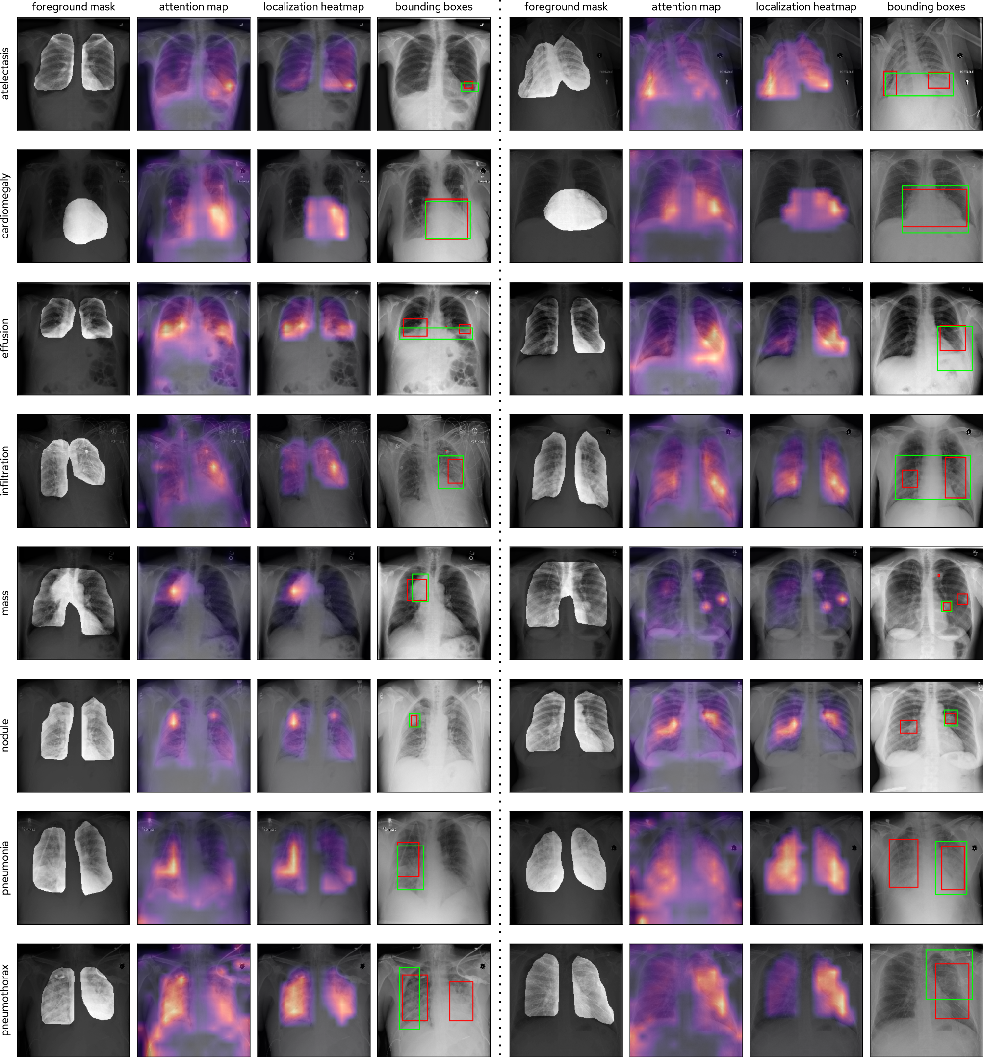
Some localization outputs of the CLARiTy-S-16-224 model are provided in 9. The model is able to produce highly precise heatmaps and bounding boxes for pathologies of all sizes. The foreground masks ensure heatmaps and bounding boxes are constrained to clinically relevant regions, improving accuracy.
4.4 Computing resources↩︎
The computing resources required for the CLARiTy-S-16-224 and CLARiTy-S-16-512 models and their components are given in 3. For the CLARiTy-S-16-224 model, the combination of the SegmentCAM and attention pooling modules increases the number of parameters and FLOPS over the vision transformer backbone by 24.7% and 21.3%, respectively. For the CLARiTy-S-16-512 model, the increase in parameters and FLOPS is 24.4% and 17.0%, respectively.
| Image Size | Component | Parameters | FLOPS |
|---|---|---|---|
| 224 | Vision Transformer Backbone | 21.68 M | 4.94 G |
| Attention Pooling Module | 5.38 K | 5.38 K | |
| SegmentCAM Module | 5.35 M | 1.05 G | |
| CLARiTy-S-16-224 | 27.03 M | 5.99 G | |
| 512 | Vision Transformer Backbone | 21.99 M | 32.35 G |
| Attention Pooling Module | 5.38 K | 5.38 K | |
| SegmentCAM Module | 5.35 M | 5.49 G | |
| CLARiTy-S-16-512 | 27.35 M | 37.84 G |
4.5 Ablation study↩︎
This section investigates the contributions of key components in the CLARiTy model through ablation studies on the SegmentCAM module, pretrained weights, classification loss, class token pooling, class token regularization, and the number of transformer layers for attention fusion and orthogonality enforcement. All ablations were performed on CLARiTy‑S‑16‑224. For each variant, we selected the best configuration according to the validation UDP. The chosen model is the variant that achieved the highest UDP, and reported test results correspond to this best validation model.
4.5.1 SegmentCAM↩︎
Two ablations were performed for the SegmentCAM module. Turning off the module completely (using only transformer self-attention for localization) resulted in a relative drop in UDP of 0.4%, a relative drop in MSLI of 2.2% and a relative increase in Macro AUC of 0.6% (¿tbl:tab:ablation95comparison?). The SegmentCAM module is important for accurate localization, but this comes at a small cost of classification performance. Since the foreground segmentation map is generated from the low-resolution (\(14 \times 14\)) heatmap tensor of the CLARiTy-S-16-224, there is imprecise coverage of each foreground mask over pathology-specific regions (3 9). The small unmasked pathology regions (which would have been masked with a higher resolution heatmap tensor) become suppressed with the background activation suppression methodology, thus resulting in the drop in Macro AUC.
Retaining the module but turning off the mask proximity and mask confinement losses caused significant relative drops in the Macro AUC, MSLI and UDP of 1.0%, 21.2% and 7.1%, respectively. The segmentation map supervision is necessary for the model to learn the correct foreground locations of each pathology.
4.5.2 Pretrained weights↩︎
An ablation was performed to investigate the impact of pretrained weights used for the CLARiTy-S-16-224. The ImageNet pretrained weights led to relative reductions in Macro AUC (1.8%), MSLI (14.2%) and UDP (5.6%), as shown in ¿tbl:tab:ablation95comparison?. The DINO weights, however, resulted in more discriminative patch embeddings, yielding more precise attention maps and higher classification accuracy.
4.5.3 Classification loss↩︎
An ablation experiment tested the commonly-used Multi-Label Soft Margin (MLSM) loss, and it resulted in relative drops in Macro AUC (0.6%), MSLI (4.5%), and UDP (1.7%), compared to the WBCE loss (¿tbl:tab:ablation95comparison?). The MLSM has the same definition as the WBCE in 1 , except that \(w_{ P} = w_{ N} = 1\). The WBCE loss is able to better handle rare classes in multi-label chest X-ray classification using its dynamic weighting scheme.
4.5.4 Class token pooling↩︎
An ablation was performed for the class token pooling method. The commonly-used GAP pooling yielded very similar Macro AUC compared to attention pooling (0.829 versus 0.830), however the MSLI and UDP had considerable relative drops of 17.9% and 5.4%, respectively (¿tbl:tab:ablation95comparison?). Attention pooling is superior for weakly-supervised localization because each dimension of a class token can correspond to different pathological features. With GAP pooling, all dimensions must have uniformly high activation values to positively classify a pathology [21]. For classification, the different kinds of pooling have a small impact.
4.5.5 Class token regularization↩︎
An ablation was performed on the class token regularization loss. The contrastive class token (CCT) loss from [77] resulted in a relative decrease in MSLI (5.0%) and UDP (1.3%), but a relative increase in Macro AUC (0.4%), compared to the OCT loss (¿tbl:tab:ablation95comparison?). CCT is worse for localization as the cosine similarity between class tokens can be pushed to being negative via cross-entropy, which is less ideal than zero similarity. CCT can promote opposition between the attention maps of different class tokens, while OCT promotes dissimilarity.
4.5.6 Class token regularization↩︎
An ablation was performed on the class token regularization loss. The contrastive class token (CCT) loss from [77] resulted in a relative decrease in MSLI (5.0%) and UDP (1.3%), but a relative increase in Macro AUC (0.4%), compared to the OCT loss (¿tbl:tab:ablation95comparison?).
To compute the CCT loss, the cross-entropy loss is applied between the class token similarity at each layer (4 ), and the identity matrix, where softmax is applied row-wise: \[\begin{align} \mathcal{L}_{\text{CCT}} = \frac{1}{q} \sum_{l=1}^{q} \text{CrossEntropy} \left( \boldsymbol{\mathit{\Theta}}_l, \mathbf{I}_C \right) \end{align}\] where CCT is applied to the final \(q=12\) layers of class tokens, and negative classes are masked [77].
Although CCT improves classification performance marginally, it degrades localization. This can be attributed to the nature of the contrastive objective: the cross-entropy formulation encourages class token embeddings to have cosine similarity significantly lower than zero, potentially pushing embeddings into opposing hemispheres of the hyperspherical space. In contrast, the OCT loss explicitly targets zero cosine similarity, enforcing orthogonality without inducing active repulsion. Consequently, CCT may over-separate class-specific attention patterns, leading to antagonistic rather than merely dissimilar attention maps, whereas OCT promotes strict dissimilarity while preserving angular equidistance in the embedding space.
4.5.7 Number of transformer layers \(p\) and \(q\)↩︎
An ablation was performed on the number of layers \(p\) to fuse for the attention maps, and the number of layers \(q\) to apply the orthogonal class token loss. A sweep over all tuples \(\left( p,q \right)\) where \(p \in \{ 1, 2, \dots , 12 \}\) and \(q \in \{ 0, 1, \dots , 12 \}\), and evaluating the validation UDP, proved that the best configuration is \(\left( 8,8 \right)\).


10 shows how the validation UDP (maximized over all \(p\)) varies with \(q\). Applying the OCT loss to \(q \leq 4\) decreases model performance compared to not applying the loss to any layers. The UDP peaks at \(q=8\) and there is a downward trend for \(q \geq 9\). This shows that the early transformer layers tend to extract features common across pathologies, while the later layers tend to extract pathology-specific features.
11 shows how the validation UDP varies with \(p\) when \(q\) is fixed at 8. Generally, fusing together more attention maps leads to better performance, until \(p=8\). When \(p > 10\), performance degrades significantly, which shows that the early transformer layers have high attention in regions non-specific to individual pathologies.
5 Discussion↩︎
CLARiTy addresses key limitations in CXR pathology analysis by integrating multi-label classification with weakly-supervised localization in a unified vision transformer framework. Our results demonstrate superior localization performance, with CLARiTy-S-16-512 achieving a Macro IoU Accuracy of 0.318 at \(\text{T(IoU)} = 0.5\), surpassing ThoraX-PriorNet-512 (0.217) and PCAN (0.103) by 46.5% and 209%, respectively, on the NIH test set. This improvement stems from class-specific attention maps fused across transformer layers, which capture pathology-specific features more discriminatively than CNN-based CAM methods [21], [45]. Notably, gains are pronounced for small pathologies like nodules and masses, where low-resolution heatmaps in prior ViT hybrids [57] falter. Classification remains competitive, with a Macro AUC of 0.818, close to state-of-the-art (0.847 for ThoraX-PriorNet-512, 0.830 for PCAN), highlighting the model’s balanced proficiency as quantified by UDP (0.594 peak in ablations).
The CLARiTy-S-16-224 variant demonstrates high efficiency at lower input resolutions, achieving a Macro AUC of 0.799 and Macro IoU Accuracy of 0.303 at \(\text{T(IoU)} = 0.5\). While scaling to 512 resolution yields modest gains (+2.4% AUC, +5.0% IoU), the 224 model decisively outperforms baselines like ThoraX-PriorNet-224 (0.201 IoU, +50.7% gain) and RGT (0.090 IoU, +236% gain), even for small pathologies such as nodules and masses. This efficiency is potentially advantageous for low-resource settings, enabling deployment on devices with limited computational power without substantial performance trade-offs.
However, fair comparisons are complicated by inconsistencies in dataset splits. Models such as RGT [57], MLRFNet [63], ThoraX-PriorNet [35], and HydraViT [54] could not be verified as using the official NIH patient-wise split, which can yield inflated performance gains—up to 10.8% absolute Macro AUC as shown in related works [33], [37]. This underscores the need for standardized evaluation protocols to ensure reproducibility and generalizability.
The SegmentCAM module in CLARiTy is pivotal, enforcing anatomical priors to suppress background activations and refine foreground masks, yielding a 2.2% MSLI boost in ablations. This could mitigate shortcut learning, a prevalent issue in NLP-labeled datasets [9], by constraining predictions to clinically plausible regions—e.g., lungs for atelectasis. The orthogonal class token loss further promotes token dissimilarity, improving MSLI by 5.0% over contrastive alternatives, while attention pooling allows dimension-specific feature encoding, outperforming GAP by 17.9% in MSLI. DINO pretraining enhances discriminative embeddings, contributing 14.2% MSLI gain versus ImageNet, aligning with findings on self-supervised benefits for medical tasks [18].
Compared to related works, CLARiTy advances beyond CNN-ViT hybrids [45], [54] by leveraging pure ViT self-attention for localization without gradient-based CAM, while reducing noise in heatmaps [17]. It also outperforms location-aware and multi-resolution pyramidal methods [33], [44] in handling complex pathologies via multi-token design. Anatomical priors echo ThoraX-PriorNet [35] but are integrated more seamlessly via SegmentCAM, avoiding separate segmentation networks.
Limitations include reliance on the NIH dataset, which may embed biases from NLP labels and demographic skews [10]. While patient-wise splits mitigate leakage, external validation on datasets like CheXpert or MIMIC-CXR could confirm generalizability. Heatmaps enhance explainability, but clinical validation by radiologists is needed to assess utility in bias detection.
Future work could extend CLARiTy to 3D CT scans or multimodal inputs (such as radiological reports via TieNet [26]), incorporate uncertainty estimation for rare pathologies, or fine-tune on underrepresented demographics to address ethical concerns. Overall, CLARiTy’s label-efficiency and precision position it as a robust tool for automated CXR screening, with potential uses in resource-limited settings.
6 Conclusion↩︎
In conclusion, CLARiTy represents a significant advancement in automated CXR analysis, enabling joint multi-label pathology classification and weakly-supervised localization using only image-level labels and anatomical priors. By leveraging multiple class tokens, SegmentCAM for prior-guided background suppression, orthogonal regularization, and attention pooling in a vision transformer, CLARiTy achieves state-of-the-art localization (50.7% relative Macro IoU Accuracy gain over priors) while maintaining strong classification on the NIH benchmark. An ablation study confirms each component’s contributions to improved classification and localization performance. These advances yield interpretable heatmaps that could facilitate the detection of biases and shortcut learning, thereby supporting more reliable computer-aided detection systems in clinical practice. Future extensions to diverse datasets and modalities will further broaden the impact of CLARiTy.
Declaration of competing interest↩︎
The authors declare that they have no known competing financial interests or personal relationships that could have appeared to influence the work reported in this paper.
CRediT authorship contribution statement↩︎
John M. Statheros: Conceptualization, Methodology, Software, Validation, Formal Analysis, Investigation, Data Curation, Writing – Original Draft, Visualization. Hairong Bau: Conceptualization, Methodology, Writing – Review & Editing, Supervision. Richard Klein: Conceptualization, Methodology, Writing – Review & Editing, Supervision.
Data availability↩︎
The NIH ChestX-ray14 dataset is available at https://nihcc.app.box.com/v/ChestXray-NIHCC.
Computer code↩︎
Code for models and scripts will be available upon publication.
Acknowledgments↩︎
Funding for infrastructure related to this work was provided by the Canadian Institutes of Health Research (CIHR) under project grant titled “Using locally developed computer-assisted detection to promote social justice for a population with a high burden of lung disease: A participatory equity-sensitive approach” (RN520904 – 506651).
Declaration of generative AI and AI-assisted technologies in the manuscript preparation process↩︎
During the preparation of this work the authors used ChatGPT and Grok in order to improve clarity and readability of prose. After using these tools, the authors reviewed and edited the content as needed and take full responsibility for the content of the published article.
7 Prompt given to Grok↩︎
I am training a segmentation-aware classification model based on the NIH ChestX-ray14 dataset. The segmentation model produces maps for the following regions: [‘Left Clavicle’, ‘Right Clavicle’, ‘Left Scapula’, ‘Right Scapula’, ‘Left Lung’, ‘Right Lung’, ‘Left Hilus Pulmonis’, ‘Right Hilus Pulmonis’, ‘Heart’, ‘Aorta’, ‘Facies Diaphragmatica’, ‘Mediastinum’, ‘Weasand’, ‘Spine’]. The labels for the ChestX-ray14 dataset are: [‘Atelectasis’, ‘Cardiomegaly’, ‘Consolidation’, ‘Edema’, ‘Effusion’, ‘Emphysema’, ‘Fibrosis’, ‘Hernia’, ‘Infiltration’, ‘Mass’, ‘Nodule’, ‘Pleural Thickening’, ‘Pneumonia’, ‘Pneumothorax’]. Tell me, which segmentation regions do I need for each pathology? In other words, where would I find these pathologies in a chest X-ray from the regions given to you?