Dissipation due to bulk localized low-energy modes in strongly disordered superconductors
December 12, 2025
Abstract
Strongly disordered superconductors (SDSCs) are widely used in qubits, microwave resonators, photon detectors, and other superconducting quantum devices. In SDSC-based devices, coherence times are limited by low-temperature microwave dissipation in the material. However, the standard Mattis–Bardeen theory fails in SDSCs because their single-particle spectrum exhibits a hard pseudogap \(\Delta_{P}\) both below and above the transition temperature \(T_{c}\). We develop a novel microscopic theory of the dependence of ac dissipation in such systems on temperature \(T\) and frequency \(\omega\). We analyze the resonator quality factor \(Q(\omega,T)\) in the practically relevant range \(\hbar\omega,\,T\ll\Delta\leq\Delta_{P}\), where \(\Delta\) is the typical superconducting order parameter, distinct from \(\Delta_{P}\). We show that low-\(\omega\) dissipation is dominated by a new type of bulk localized collective modes arising from spatial inhomogeneity of the superconducting state. Consequently, \(Q(\omega)\) decreases strongly with \(\omega\) and exhibits two-level-system-like growth with \(T\) for \(T\ll T_{c}\). Our theory provides a microscopic understanding of existing and future experiments on thin films of \(\mathrm{InO}_{x}\), TiN, NbN, and similar SDSCs, and is phenomenologically relevant to granular aluminum films. The results suggest strategies to mitigate intrinsic microwave losses in SDSC-based quantum devices.
0.0.0.1 Introduction.
Superconducting quantum circuits rely on a simple promise: at microwave frequencies and at temperatures well below the superconducting gap, a superconductor should behave as an almost lossless inductor. In conventional \(s\)-wave superconductors this expectation is formalized by Mattis–Bardeen theory [1], which predicts an exponentially small dissipative conductivity, \(\text{Re}\,\sigma\), while disorder increases the sheet kinetic inductance \(L_{K}\). This makes disordered films a powerful route to high-impedance quantum circuits, compact resonators, enhanced zero-point voltage fluctuations, and protected-qubit or detector architectures [2]–[14]. The same route, however, exposes a central materials problem: increasing \(L_{K}\) is often accompanied by an excess of conductive loss, as seen in a recent survey of the microwave quality factor \(Q\) of superconducting quantum devices [15]. Understanding the microscopic origin of this intrinsic loss is therefore essential both for the physics of disordered superconductivity and for the engineering of coherent quantum circuits.
Strongly disordered superconductors (SDSCs) are not merely dirty versions of ordinary BCS metals [16], [17]. Close to the superconductor–insulator transition, amorphous films such as \(\mathrm{InO}_{x}\), TiN, and NbN develop a hard single-particle pseudogap \(\Delta_{P}\) that can persist well above the superconducting transition temperature \(T_{c}\) [17]. This pseudogap signals the formation of spatially localized Cooper pairs before global phase coherence is established. Below \(T_{c}\), the superconducting order parameter is itself strongly inhomogeneous [18]–[20]: its local magnitude has a broad distribution, with rare regions where the gap is much smaller than its typical value [16], [21], [22]. As a result, the low-energy electromagnetic response of an SDSC cannot be inferred by simply adding disorder to the Mattis–Bardeen quasiparticle picture. The relevant low-energy degrees of freedom may instead live inside the Cooper-pair sector of an inhomogeneous condensate.
This distinction is sharpened by recent microwave experiments [23]. Thin films of amorphous \(\mathrm{InO}_{x}\) can reach extremely large kinetic inductance, up to \(L_{K}\approx17\,\mathrm{nH}/\square\), but at the cost of a strongly suppressed resonator quality factor [15], [23], [24]. The usual extrinsic explanations are unsatisfactory in this regime: surface dielectric loss is inconsistent with the weak dependence on electric-field participation ratio [24], atomic two-level systems have no natural reason to track the electronic disorder so sharply, and conventional thermal or nonequilibrium quasiparticles cannot account for the magnitude and disorder dependence of the loss in the presence of a large pseudogap [15], [16], [19]. The basic unresolved question is therefore simple and experimentally pressing: what microscopic objects absorb microwave photons with \(\hbar\omega,\,T\ll\Delta\leq\Delta_{P}\) in a pseudogapped superconductor?
Previous theoretical work on SDSCs established the static ingredients needed to address this question: a pseudospin description of localized preformed Cooper pairs, a broad distribution of the local order parameter, and rare “weak spots” that strongly affect the temperature dependence of the superfluid stiffness [16], [21], [25]. What remained missing was the dynamical step: identifying the finite-frequency modes of this inhomogeneous condensate, computing their contribution to \(\text{Re}\,\sigma(\omega,T)\), and relating the result directly to the measured resonator quality factor \(Q\). In this Letter, we perform this step. We show that rare weak spots host localized collective modes corresponding to low-energy rearrangements of Cooper pairs, with an electric dipole moment set by the weak-spot size rather than by pair breaking. These modes produce a bulk dissipative response with a two-level-system-like factor \(\tanh(\hbar\omega/2T)\) and a strong frequency dependence controlled by the low-value tail of the order-parameter distribution \(P(\Delta)\), leading to a rapid drop of \(Q\) with increasing \(\omega\). The resulting expression for \(Q(\omega,T)\) explains the main trends observed in \(\mathrm{InO}_{x}\) resonators and turns microwave spectroscopy into a probe of the order parameter distribution of the rare weak regions that control dissipation in SDSCs.
0.0.0.2 A microscopic model of a SDSC.
The starting point of the microscopic model is the pseudospin Hamiltonian describing localized preformed Cooper pairs that experience phonon-induced attraction in the Cooper channel [16], [22], [26], [27]: \[\begin{align} H & =-\sum_{j}(\xi_{j}+e\phi_{j})2S^{z}_{j}\nonumber \\ & -\sum_{jk}D_{jk}\left[S^{+}_{j}S^{-}_{k}e^{-i\frac{2e}{c}A_{j\rightarrow k}}+S^{-}_{j}S^{+}_{k}e^{i\frac{2e}{c}A_{j\rightarrow k}}\right]. \label{eq:pseudospin-hamiltonian} \end{align}\tag{1}\] Here, \(j,k\) enumerate Anderson-localized single-particle states, with state \(j\) characterized by energy \(\xi_{j}\) and wave function \(\psi_{j}(\boldsymbol{r})\); \(D_{jk}=\intop d^{3}\boldsymbol{r}\,D\left(\xi_{k}-\xi_{j}\right)|\psi_{k}(\boldsymbol{r})|^{2}|\psi_{j}(\boldsymbol{r})|^{2}\) is the matrix element of the local Cooper attraction, \(D(\omega;\boldsymbol{r},\boldsymbol{r}')\approx D(\omega)\,\delta(\boldsymbol{r}-\boldsymbol{r}')\). The pseudo-spin operators \(S^{z}_{i},\,S^{\pm}_{i}\) provide a compact encoding 1 of the absence of unpaired electrons at low temperatures due to a large pseudogap [16], [22]. The interaction term in Eq. (1 ) therefore induces tunneling of preformed Cooper pairs between different localized states.
In what follows, we assume \(\xi_{i}\) to be independent random variables distributed according to a broad distribution \(P_{\xi}(\xi)\), with a finite density at the Fermi level, \(P_{0}:=P_{\xi}(\xi=0)=\nu_{0}/n\), where \(\nu_{0}\) is the single-particle density of states (DoS) per spin projection, and \(n\) is the electron concentration. The set of sites \(i\) and of pairs \(\langle ij\rangle\) for which \(D_{ij}>0\) can then be viewed as an interaction graph. Due to strong statistical fluctuations of \(D_{ij}\), this graph is sparse [16], [25]. As a result, the immediate vicinity of each vertex is locally tree-like with a certain average branching number \(K\), whereas at large scales, loops inevitably appear as a consequence of the embedding of this graph into 3D Euclidean space. However, these loops almost surely contain at least \(m_{\text{tree}}\sim\ln\left\{ 2\nu_{0}r^{3}_{\text{loc}}\omega_{D}\right\} /\ln K\gg1\) sites, where \(r_{\text{loc}}\) is the localization length of the electron wave functions \(\psi_{i}(\boldsymbol{r})\), and \(\omega_{D}\) is the energy cutoff of the Cooper pair attraction. The quantity \(m_{\text{tree}}\) thus describes the spatial extent of the locally tree-like structure.
Although the statistical distribution of \(D_{ij}\) in a real system is likely rather nontrivial [16], we restrict ourselves to the following simple model: for a given \(i\), \(D_{ij}=0\) for all \(j\) except \(K+1\) randomly selected neighbors within the localization volume with equal probability, for which with \(D_{ij}=\text{const}=\lambda/(2P_{0}K)\). This relation also defines the dimensionless Cooper-pair coupling constant \(\lambda\). This approximation is expected [21] to be qualitatively correct for low-energy physics unless the true \(D_{ij}\) distribution is broad.
The mean-field treatment of Hamiltonian (1 ) defines [21] the superconducting energy scale \(\Delta_{0}\sim2\omega_{D}e^{-1/\lambda}\), where, in a more realistic model of \(D_{ij}\) [16], the exponential changes to a power-law dependence, \(\Delta_{0}\propto\lambda^{1/\gamma}\) with \(\gamma\approx0.57\). Although the true order parameter is strongly inhomogeneous at the scale of the coherence length [19], [21], [27], \(\Delta_{0}\) provides a relevant energy scale. In particular, it allows one to define the dimensionless disorder strength \(\kappa=\overline{D_{ij}}/\Delta_{0}\), which turns out to be the key measure of the competition between disorder and superconductivity [21], [25]: \(\kappa\ll1\) corresponds to a nearly homogeneous superconducting state, whereas for \(\kappa\gg1\) the model exhibits a broad distribution of the order parameter that becomes fat-tailed when \(\kappa\ge\kappa_{1}=\exp\left\{ \frac{1}{2\lambda}\right\} \gg1\), with the disorder-induced superconductor-insulator transition (SIT) occurring at \(\kappa_{c}\gg\kappa_{1}\) [22]. Henceforth, the condition \(\kappa\ll\kappa_{1}\) is assumed.
Hamiltonian (1 ) features minimal (gauge) coupling to the discrete electromagnetic potentials \(\phi_{i}\), \(A_{i\rightarrow j}=-A_{j\rightarrow i}\). As a consequence of the discrete nature of the model, these potentials are defined on each site and on each directed edge, respectively. In the absence of external vector potential, the current operator along a given edge \(i\to j\) is given by \[I_{i\rightarrow j}=-c\,\frac{\partial H}{\partial A_{i\rightarrow j}}=8eD_{ij}\left(S^{x}_{i}S^{y}_{j}-S^{x}_{j}S^{y}_{i}\right). \label{eq:current-op-def}\tag{2}\] Note that \(I_{i\rightarrow j}\) is a 4-particle operator in terms of original electronic operators, expressing the fact that the charge transport in the model occurs only because of the interaction. The connection between \(\phi_{i},\,A_{i\rightarrow j}\) and the real-space electromagnetic potentials \(\phi(\boldsymbol{r}),\,\boldsymbol{A}(\boldsymbol{r})\) is given by [25] \(\phi_{i}=\intop d^{3}\boldsymbol{r}|\psi_{i}(\boldsymbol{r})|^{2}\phi(\boldsymbol{r})\), and \(A_{i\rightarrow j}=\intop d^{3}\boldsymbol{r}\,\boldsymbol{\mathfrak{D}}_{i\rightarrow j}(\boldsymbol{r})\cdot\boldsymbol{A}(\boldsymbol{r})\), where the field \(\boldsymbol{\mathfrak{D}}_{i\rightarrow j}(\boldsymbol{r})\) is expressed in terms of variational derivatives of \(D_{ij}\) with respect to external vector potential [28]. The \(\boldsymbol{\mathfrak{D}}\) field has the physical meaning of the current density induced by tunneling of a Cooper pair from one localized site to another, \(\boldsymbol{j}(\boldsymbol{r})=I_{i\rightarrow j}\,\boldsymbol{\mathfrak{D}}_{i\rightarrow j}(\boldsymbol{r})\). Importantly, charge conservation in real space implies [25] that \(\left|\psi_{j}(\boldsymbol{r})\right|^{2}-\left|\psi_{i}(\boldsymbol{r})\right|^{2}=\nabla\cdot\boldsymbol{\mathfrak{D}}_{i\rightarrow j}(\boldsymbol{r})\).
The key quantity describing the low-frequency conductivity is the retarded local current correlator \(R_{ij}\): \[R_{ij}(\omega)=(2e)^{2}\left\langle N_{ij}\right\rangle -\intop^{+\infty}_{0}dt\,ie^{i\omega t}\left\langle \left[I_{i\to j}(t),I_{i\to j}(0)\right]\right\rangle , \label{eq:current-correlator95def}\tag{3}\] where \(N_{ij}=8eD_{ij}\left(S^{x}_{i}S^{x}_{j}+S^{y}_{j}S^{y}_{i}\right)\) is the appropriate diamagnetic term.
0.0.0.3 Solution by Belief Propagation.
To describe microscopic physical quantities, such as \(R_{ij}\), we employ the classical Belief Propagation [25], as suggested by the locally tree-like structure of the interaction graph. This approach expresses local physical quantities in terms of the eigenproblem of a certain two-spin Hamiltonian: \[\begin{align} H_{\left\langle ij\right\rangle } & =-\sum_{n=i,j}2\xi_{n}S^{z}_{n}-4D_{ij}\left(S^{x}_{i}S^{x}_{j}+S^{y}_{i}S^{y}_{j}\right)\nonumber \\ & -\sum_{\alpha=x,y}\left(2h^{\alpha}_{i\rightarrow j}S^{\alpha}_{j}+2h^{\alpha}_{j\rightarrow i}S^{\alpha}_{i}\right). \label{eq:two-sping95effective95Hamiltonian} \end{align}\tag{4}\] This Hamiltonian contains the local disorder \(\xi_{i},\,\xi_{j}\) and the order parameter fields \(h_{i\rightarrow j},\,h_{j\rightarrow i}\), which encode the local environment of the target edge \(\left\langle ij\right\rangle\). The fields \(h_{k\rightarrow i}\) are obtained by solving the self-consistency equation for each directed edge \(k\rightarrow i\): \[h_{k\rightarrow i}=\sum_{j\in\partial i\backslash\left\{ k\right\} }D_{ij}\frac{h_{j\rightarrow i}}{B_{j\rightarrow i}}\,\tanh\frac{B_{j\rightarrow i}}{T}, \label{eq:h-equations}\tag{5}\] where \(B_{j\rightarrow i}=\sqrt{\xi^{2}_{j}+h^{2}_{j\rightarrow i}}\), and the sum over \(j\) runs over all neighbors of \(i\) except \(k\). Note that, due to the directedness of Eq. (5 ), quantities with permuted vertex indices, e.g. \(h_{i\to j}\) and \(h_{j\to i}\), are not equivalent.
Any physical quantity associated with a pair \(\left\langle ij\right\rangle\) of adjacent sites (see, e.g., Eq. (10 )) is expressed through the eigenpairs \(\left\{ E^{(n)}_{ij},\left|n_{ij}\right\rangle \right\} ,\,n=1,...,4\) of Hamiltonian (4 ) with the corresponding values of \(\left\{ \xi_{i},\,\xi_{j},\,h_{i\rightarrow j},\,h_{j\rightarrow i},\,D_{ij}\right\}\). Using Eq. (5 ), one can express expectation values of quantities on site \(j\) in a form that makes explicit the equivalence and directedness of each edge incident to \(j\). An example is Eq. (35) of Ref. [25] for the onsite order parameter \(\Delta_{j}\), encoding the anomalous expectation \(\left\langle S^{-}_{j}\right\rangle\). However, it is the set of fields \(h_{i\to j}\) on each directed edge that encodes the complete statistical information, which is why we focus exclusively on \(h_{i\to j}\). Moreover, it can be shown [25] that the statistics and physical properties of \(h_{i\to j}\) closely resemble those of \(\Delta_{j}\), justifying mild abuse of the term “order parameter” in reference to \(h_{i\to j}\).
0.0.0.4 An approximate expression for \(\text{Re}\sigma\) and the Network Model.
Applying a macroscopic superconducting phase gradient \(\nabla\varphi\) (e.g., as a boundary condition at the sample edges) creates a microscopic distribution of phase \(\varphi\) at each site, governed by the response equations and charge conservation [25]. The real part of the conductivity is derived from the total Joule heat: \(P=\frac{1}{2}\intop d^{3}\boldsymbol{r}\,\text{Re}\sigma(\omega)\,\left|\boldsymbol{E}(\boldsymbol{r})\right|^{2}\), where \(\boldsymbol{E}(\boldsymbol{r})=-i\omega\frac{\nabla\varphi}{2e}\) is the external electric field. In terms of edge currents \(I_{i\to j}\), the dissipated power is given by a sum of contributions from each undirected edge \(\left\langle jk\right\rangle\), \[P=\frac{1}{2}\frac{1}{2e}\sum_{\left\langle jk\right\rangle }\text{Re}\left\{ -i\omega I^{*}_{k\to j}\left(\varphi_{j}-\varphi_{k}\right)\right\} .\] At frequency \(\omega\) such that \(\omega/\Delta_{0}\ll1\), the current response can be represented as [25]2 \[I_{i\to j}=\frac{1}{e}\,R_{ij}(\omega)\,\left(\varphi_{j}-\varphi_{i}\right), \label{eq:edge-current-response95functional-form}\tag{6}\] where \(R_{ij}\) is given by Eq. (3 ).
Moreover, at low frequencies, \(R_{ij}\) is almost purely real, except for rare instances where the dissipative response contains a resonance at sufficiently low frequencies, introducing a finite imaginary contribution to the current from the first term of Eq. (6 ). Since these instances are rare, the change in the distribution of phases \(\varphi_{j}\) due to the finite imaginary part of \(R_{ij}\) can be neglected, and one can use the phase distribution from the \(\omega=0\) case, where the response is purely superconducting. The real part of the conductivity, \(\text{Re}\sigma(\omega)\), is then expressed as \[\text{Re}\sigma(\omega)\approx n_{\text{e}}\,\frac{2}{\omega}\,\overline{\text{Im}R_{ij}(\omega)\,\frac{\left(\varphi_{j}-\varphi_{i}\right)^{2}}{\left(\overline{\nabla\varphi}\right)^{2}}}. \label{eq:real-conductivity95via95local-response}\tag{7}\] Here, \(n_{\text{e}}=n\left\langle K+1\right\rangle /2\) is the concentration of undirected edges, the overline denotes averaging over all disorder configurations, and \(\varphi_{i}\) are the phases in the \(\omega=0\) static problem with the mean phase gradient \(\overline{\nabla\varphi}\) (see Ref. [25]).
Eq. (7 ) provides an approximate numerical method for computing the macroscopic real conductivity. To this end, we employ an extended version of the protocol of Ref. [25], henceforth referred to as the network model (NM): i) generate a large instance of a locally tree-like graph and disorder fields \(\xi_{i}\), ii) solve the self-consistency Eq. (5 ) for the order parameter fields \(h_{i\to j}\) on each directed edge, iii) compute the local responses \(R_{ij}\) according to Eqs. (2 )-(4 ) for each edge \(\left\langle ij\right\rangle\), iv) numerically solve the Kirchhoff equations for the superconducting phases \(\varphi_{i}\) with a given phase difference \(\varphi_{\text{right}}-\varphi_{\text{left}}=|\nabla\varphi|\times L\) in a geometry of a two-dimensional 3 brick of size \(L\times w\) (see Ref. [25] for details), and v) compute the required averages, such as Eq. (7 ), using the resulting large sample of \(R_{ij}\) and \((\varphi_{j}-\varphi_{i})\). This procedure is repeated for multiple disorder realizations to ensure a proper disorder average.
0.0.0.5 Approximate analytical solution.
Directly computing the average in Eq. (7 ) requires the joint probability distribution of \(\text{Im}R_{ij}(\omega)\) and \(\left(\varphi_{j}-\varphi_{i}\right)^{2}\). This distribution is only accessible via the numerical solution of the NM. Remarkably, the following approximate relation holds: \[\text{Re}\sigma\left(\omega\ll\Delta_{0}\right)\approx\frac{2\eta\,n_{\text{e}}\overline{\left(\boldsymbol{r}_{i}-\boldsymbol{r}_{j}\right)^{2}}/\mathcal{D}}{\omega}\,\overline{\text{Im}R_{ij}(\omega)}, \label{eq:low-freq-conductivity95via95average-imaginary-response}\tag{8}\] where \(\overline{\left(\boldsymbol{r}_{i}-\boldsymbol{r}_{j}\right)^{2}}=\frac{\mathcal{D}}{\mathcal{D}+2}r^{2}_{\text{loc}}\) for the present model in \(\text{\mathcal{D}}\) spatial dimensions, and the dimensionless coefficient \(\eta\) is nearly independent of frequency. This relation is especially striking given that both its sides are steep functions of frequency, as will be shown below. The qualitative reason behind Eq. (8 ) is that \(\text{Re}\sigma\) is dominated by the density of low-energy excitations: \[\text{Re}\sigma(\omega)\sim\overline{\delta\left(\omega-\Omega_{ij}\right)},\,\,\,\Omega_{ij}=\min_{n\neq m}\left|E^{(n)}_{ij}-E^{(m)}_{ij}\right|, \label{eq:sigma-estimation95via-lowest-excitation-frequency}\tag{9}\] where \(E^{(n)}_{ij}\) are the eigenenergies of \(H_{\left\langle ij\right\rangle },\)Eq. (1 ), and \(\Omega_{ij}\) is the minimal transition frequency for a given edge \(\left\langle ij\right\rangle\). As will be shown below, the spectral density of \(\Omega_{ij}\) exhibits a steep exponential dependence on frequency. On the other hand, the average of the squared current matrix element and phase difference in Eq. (7 ) carries at most a weak power-law dependence on \(\omega\), see for details.
One further expects that the main temperature dependence is reproduced in Eq. (8 ). Indeed, finite temperature causes only a small change in the superfluid stiffness, \(\delta\Theta/\Theta\ll1\) [25], suggesting a similarly small change in the phase differences \(\varphi_{j}-\varphi_{i}\) and, consequently, in the value of \(\eta\) in Eq. (8 ), viz. \(\delta\eta/\eta\sim\delta\Theta/\Theta\ll1\). However, one cannot fully exclude that the temperature-dependent part of the correlations between \(\text{Im}R_{ij}\) and \((\varphi_{j}-\varphi_{i})\) is much more pronounced among the strongly dissipating edges. A discussion of this aspect is also presented in .
In addition, the numerical solution of the NM unambiguously demonstrates a noticeable \(\kappa\) dependence of \(\eta\) (see ). Because of the approximate character of Eq. (8 ), we do not conduct a detailed numerical analysis of this dependence. However, the discussion of the \(\omega,\,T\)-dependencies of \(\text{Re}\sigma\) remains qualitatively valid.
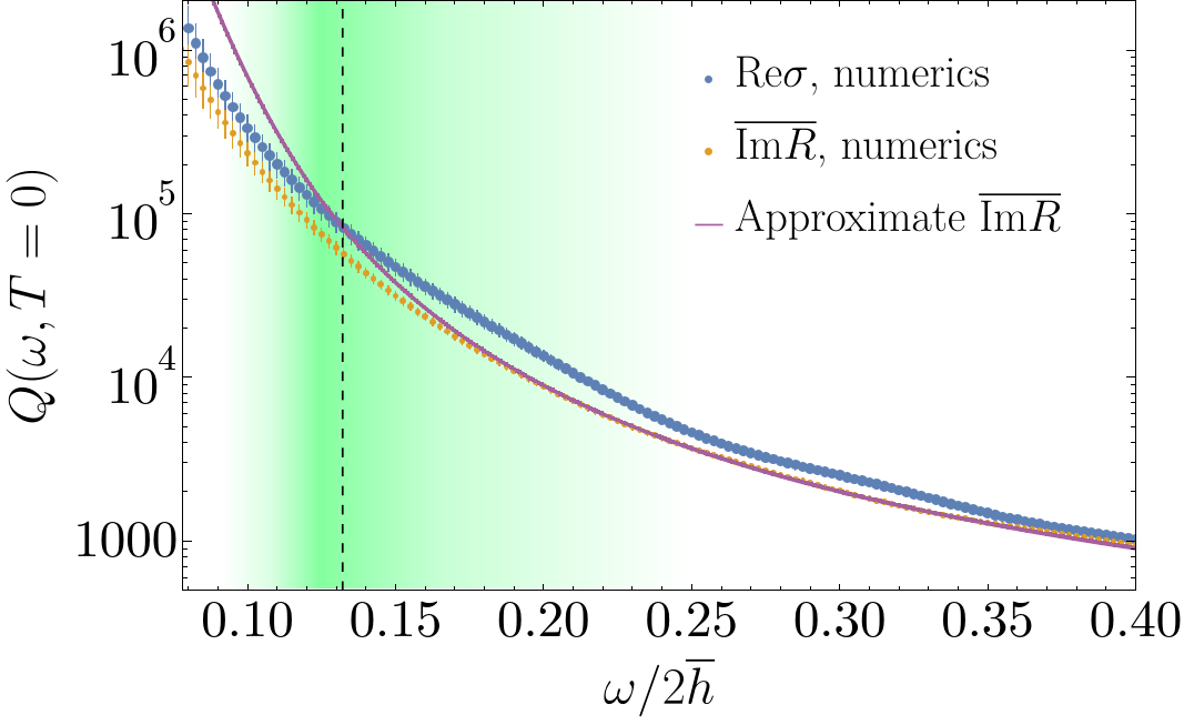
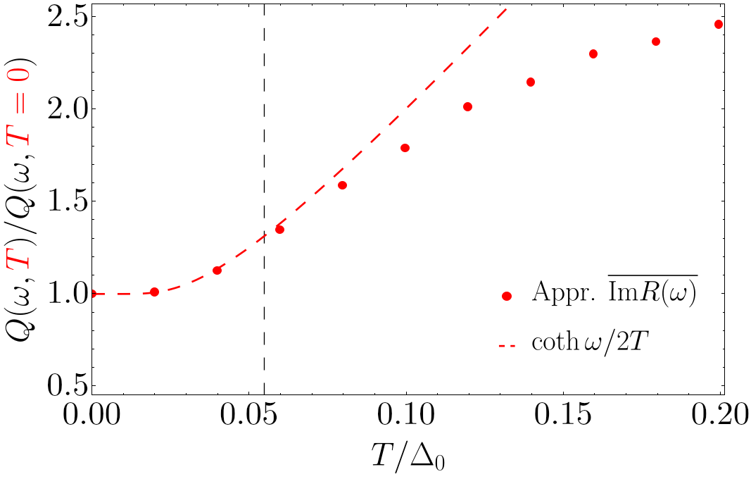
Figure 1: The behavior of the resonator quality factor \(Q\propto\omega/\text{Re}\sigma\)in the pseudospin model with \(K=10\), \(\kappa=10\), \(\lambda\approx0.1373\).Left: Dependence of \(Q\) on frequency \(\omega\). Blue andorange dots correspond to the data from \(M=20\) realizations of theNM of size \(N\approx10^{6}\) with \(r_{\text{loc}}/a=48.27\) (where\(a\) is the mean inter-site distance in real space), while the solidpurple line corresponds to Eq. (12 ),with \(P(h)\) found by population dynamics. To determine \(\eta\),Eq. (8 )was fitted on a broader frequency interval, \(\omega/2\overline{h}\in\left[0.08,1\right]\),causing low-frequency values of the approximation (orange) to be systematicallylower than the NM values (blue). The vertical dashed line correspondsto \(\omega=0.109\,\Delta_{0}\). The green region marks the range ofvalues that corresponds to the experimental data [23], [24],with \(T_{c}=1.4\,\text{K}\) and \(\omega=3.85\,\text{GHz}\). The uncertaintystems from the unaccounted-for quasiparticle suppression of the measured\(T_{c}\) relative to the model-predicted \(T^{(0)}_{c}\approx2.4\,\overline{h}\) [25].The color intensity conveys the probability of a given \(\omega/2\overline{h}\).Right: Temperature dependence of \(Q\), normalized to its valueat \(T=0\), for \(\omega=0.109\,\Delta_{0}\). Points correspond to Eq. (12 ),with \(P(h)\) found from population dynamics. The vertical dashed linedenotes \(\omega=2T\)..
\(\text{Im}R_{ij}(\omega>0)\) is expressed [25] in terms of the eigenpairs \(\left\{ E^{(n)}_{ij},\left|n_{ij}\right\rangle \right\}\) of the two-spin Hamiltonian (4 ): \[\text{Im}R_{ij}(\omega)=\sum_{n\neq m}\left|I^{(mn)}_{ij}\right|^{2}W^{(nm)}_{ij}\,\frac{\pi}{2}\delta\left(\omega-\Omega^{(mn)}_{ij}\right), \label{eq:Im-R95particular-disorder-realization}\tag{10}\] where \(W^{(nm)}_{ij}=\left(e^{-E^{(n)}_{ij}/T}-e^{-E^{(m)}_{ij}/T}\right)/\sum_{m}e^{-E^{(m)}_{ij}/T}\), \(I^{(mn)}_{ij}=\left\langle m_{ij}\left|I_{i\rightarrow j}\right|n_{ij}\right\rangle\), and \(\Omega^{(mn)}_{ij}=E^{(m)}_{ij}-E^{(n)}_{ij}\). The average \(\overline{\text{Im}R_{ij}(\omega)}\) is then obtained by averaging Eq. (10 ) over the ensemble of effective two-spin Hamiltonians obtained by sampling \(\left\{ \xi_{i},\,\xi_{j},\,h_{i\rightarrow j},\,h_{j\rightarrow i},\,D_{ij}\right\}\) (see Ref. [25]). The averaging procedure entails two technical complications: i) diagonalizing of \(H_{\left\langle ij\right\rangle }\) for each realization, and ii) smoothing the \(\delta\)-function in \(\text{Im}R_{ij}\). The details of the associated numerical routine are presented in Ref. [28].
In the limit \(\omega\ll\overline{h}\), where \(\overline{h}\) is the mean value of the order parameter, the averaging can be performed analytically: \[\frac{\overline{\text{Im}R_{ij}(\omega)}}{\tilde{R}}=\frac{\omega}{2\Delta_{0}}\tanh\frac{\omega}{2T}\intop^{\omega/2}_{0}dhP(h)\arccos\frac{2h}{\omega}. \label{eq:local-response95via95order-parameter-distribution}\tag{11}\] Here, \(\tilde{R}=\frac{\pi\kappa}{2}\left(2P_{0}\Delta_{0}\right)^{2}(2e)^{2}\overline{h}\), and \(P(h)\) stands for the probability density of the order parameter \(h_{i\to j}\). This result expresses the fact that the relevant disorder configurations are identical to those causing the temperature suppression of the order parameter [25]. The derivation is detailed in Ref. [28], see also .
Importantly, Eq. (11 ) contains two sources of temperature dependence: i) the occupation number \(\tanh\{\omega/2T\}\) of the local mode, and ii) the order parameter distribution \(P(h)\) that implicitly contains temperature. The second aspect is important because Eq. (11 ) is sensitive to the low-value tail of \(P\), which, in turn, is strongly temperature-dependent due to its steep profile [25].
From a technical point of view, Eqs. (8 ) and (11 ) reduce the computation of \(\text{Re}\sigma\) (up to a frequency- and temperature-independent constant) to the problem of finding \(P(h)\). This problem can be efficiently addressed by population dynamics, which amounts to finding \(P(h)\) such that the distributions of left and right sides of Eq. (5 ) are equal. Ref. [28] contains a brief review of the corresponding numerical routine, while a more detailed exposition of the associated analytical techniques can be found in Ref. [25].
0.0.0.6 Resonator quality factor as an experimental probe of the order parameter distribution.
With the help of Eqs. (8 ) and (11 ), the inverse low-frequency quality factor of a resonator made of a SDSC can be expressed as [23], [24] \[\frac{1}{Q}=\frac{\text{Re}\sigma}{\text{Im}\sigma}=C\frac{\omega}{2\Delta_{0}}\tanh\frac{\omega}{2T}\intop^{\omega}_{0}dhP(h)\arccos\frac{2h}{\omega}, \label{eq:quality-factor95via95microscopic-response-statistics}\tag{12}\] where \(\text{Im}\sigma=(2e)^{2}\Theta/(\omega d)\) is the imaginary part of the conductivity, and \(P(h)\) is the distribution of the order parameter. The numerical coefficient \(C=2\eta\,n\overline{\left(r_{i}-r_{j}\right)^{2}}d\,\left(2P_{0}\Delta_{0}\right)^{2}\frac{\Delta_{0}}{\Theta}\,(K+1)\frac{\pi\kappa\overline{h}}{12\Delta_{0}}\) is effectively frequency- and temperature-independent (\(\Theta\) is the superfluid stiffness, \(d\) is the film’s thickness). In Eq. (12 ), one also neglects the weak dependence of the mean order parameter \(\overline{h}\) on temperature [25]. Eq. (12 ) constitutes the main result of this Letter.
shows the dependence of \(Q\) on both \(\omega,\,T\) obtained by using Eq. (11 ) for \(\overline{\text{Im}R}\). The frequency dependence is compared to the result of the numerical solution of the NM. Two important observations are in order: i) \(Q\) decreases rapidly with frequency due to the corresponding surge in the spectral density of excitations. According to Eq. (11 ), this is a direct consequence of the steep profile [21], [25] of the order parameter distribution \(P(h)\). ii) \(Q\) initially grows with temperature, reflecting thermal activation of the local degrees of freedom, corresponding to the \(\tanh\{\omega/2T\}\) factor in Eq. (11 ). However, this trend is later slowed down by the increase in the spectral density of excitations. Within Eq. (12 ), this results from the growth [25] of the low-value tail of the order parameter distribution.
Importantly, at the lowest frequencies, the left panel of displays a discrepancy between the NM and Eq. (12 ). This difference originates from the fact that the NM obtains the order parameter as the solution to the self-consistency Eq. (5 ) on a graph with a finite \(m_{\text{tree}}\), whereas Eq. (12 ) uses population dynamics to restore \(P(h)\) and thus corresponds [25] to the limit \(m_{\text{tree}}\to\infty\). Therefore, the discrepancy in signals the breakdown of Belief Propagation for low \(h\) values, as they acquire long-distance correlations, despite our best efforts 4. Our findings are thus valid for frequencies above the problematic range, whereas the qualitative picture within this range should be studied more carefully.
Eq. (12 ) and the steep profile of \(Q(\omega)\) can be exploited to experimentally probe the tail of the order parameter distribution. Namely, Eq. (11 ) can be solved for \(P(h)\), rendering \[P(h)\propto\frac{d}{dh}\intop^{2h}_{0}\frac{d\omega}{\sqrt{1-(\omega/2h)^{2}}}\,\frac{d}{d\omega}\frac{\coth\{\omega/2T\}}{\omega\,Q(\omega)}. \label{eq:order-parameter-distribution95via95quality-factor}\tag{13}\] Eq. (13 ) suggests the following protocol for restoring \(P\left(h\ll\Delta_{0}\right)\): i) measure the low-frequency quality factor for a sequence of plasmonic resonances on a thin strip resonator at low temperature, ii) calculate the integrand by differentiating a numerical interpolation of the data, iii) calculate the cumulative distribution function \(F(h)=\intop^{h}_{0}dhP(h)\) by means of numerical integration, and iv) use one more round of numerical differentiation to restore \(P(h)\) up to an overall factor. The result can further be compared to previous indirect experimental [19], [29] and numerical [30]–[32] probes of the same quantity.
0.0.0.7 Conclusions.
We analyzed the real part of conductivity, \(\text{Re}\sigma(\omega)\), in SDSCs. We demonstrated that \(\text{Re}\sigma\) at low frequency is dominated by bulk collective localized excitations. These excitations reside in the regions of local suppression of the superconducting order parameter and are thus directly linked to the intrinsic inhomogeneity of the superconducting state. The sharp profile of the spectral density of these excitations translates into a steep increase of \(\text{Re}\sigma\) with frequency, roughly following the low-value tail of the order-parameter distribution, \(P(h\ll\Delta_{0})\) [see Eq. (12 )].
Our results are in qualitative agreement with the recent experimental data [23], [24] on resonators made of \(\mathrm{InO}_{x}\). This includes both the overall magnitude of the internal resonator quality factor \(Q\propto1/\text{Re}\sigma\) and its temperature dependence (see ). To test relation (13 ) between \(Q(\omega)\) and \(P(h)\), a detailed low-temperature measurement of \(Q(\omega)\) for an SDSC-based resonator is desirable, e.g., using the technique of Refs. [23], [24].
, left, suggests improving coherence times of SDSC-based quantum devices by lowering the operating frequency. Because \(P(h)\) is steep, halving \(\omega\) can raise \(Q\) by an order of magnitude for the same film, provided the film is sufficiently disordered for the present theory to apply. This improvement is practically important for several qubit designs [2], [3], [6], [10]–[13], advancing scalable quantum computing.
Our results raise a number of physical questions beyond the technical issues of the employed simplifications. First, our analysis does not yield the spatial structure of the localized collective modes in question. Second, these excitations have been conjectured [25] to be responsible for the near-power-law suppression of the superfluid stiffness \(\Theta\) as a function of \(T\). However, directly computing \(\Theta(T)-\Theta(0)\) via the Ferrell-Glover-Tinkham relation [33] is hindered because the corresponding integral converges at frequencies comparable to the superconducting energy scales, whereas our theory is limited to much lower frequencies. Finally, the additional low-temperature entropy due to the discussed collective modes appears important [23] for the structure of the phase diagram of SDSCs near the disorder-driven quantum phase transition. At the same time, Ref. [34] demonstrates that Coulomb repulsion is essential for describing the first-order nature of this transition. A consistent treatment incorporating both ingredients will be presented elsewhere.
Some of the aforementioned experimental features were also observed [35], [36] in high-resistance granular Aluminum films. However, the electron (near-) localization in granular materials arises from their fine-grained structure, rather than from the single-particle Anderson localization [16], [26] relevant to the present work. Nevertheless, the presence of localization effects in both types of systems suggests that similar low-frequency dissipation mechanisms may be operative.
The authors would like to thank Denis Basko, Thibault Charpentier and Benjamin Sacépé for numerous fruitful discussions. A.V.K. is grateful for the support by Laboratoire d’excellence LANEF in Grenoble (ANR-10-LABX-51-01).
1 End Matter↩︎
1.0.1 Quality of the approximation for \(\text{Re}\sigma(\omega)\)↩︎
Relation (7 ) represents an empirical shortcut to the solution of the NM as it replaces all possible statistical correlations between \(\text{Im}R_{ij}(\omega')\) and \(\left(\varphi_{j}-\varphi_{i}\right)^{2}\) with a single coefficient \(\eta\). To characterize the quality of this approximation, one considers the following generalization of this coefficient: \[\eta(\omega):=\frac{\overline{\intop^{\omega}_{0}d\omega'\,\text{Im}R_{ij}(\omega')\,\left(\varphi_{j}-\varphi_{i}\right)^{2}}}{\,\overline{\intop^{\omega}_{0}d\omega'\,\text{Im}R_{ij}(\omega')}\times\left(\overline{\nabla\varphi}\right)^{2}\overline{\left(\boldsymbol{r}_{i}-\boldsymbol{r}_{j}\right)^{2}}/\mathcal{D}}, \label{eq:eta-integral-coeff}\tag{14}\] where \(\overline{\left(\boldsymbol{r}_{i}-\boldsymbol{r}_{j}\right)^{2}}=\frac{\mathcal{D}}{\mathcal{D}+2}r^{2}_{\text{loc}}\) for the simple pseudospin model in \(\mathcal{\mathcal{D}}\) spatial dimensions, \(\overline{\nabla\varphi}\) is the mean external phase gradient, and all other averages \(\overline{\bullet}\) are estimated numerically from the solution of the \(\omega=0\) NM. The integration in Eq. (14 ) is needed to facilitate the averaging procedure, since expression (10 ) for \(\text{Im}R_{ij}\) contains a \(\delta\)-function of frequency, an inconvenient object for numerical estimations.
The numerator of Eq. (14 ) is proportional to the integral \(\intop^{\omega}_{0}d\omega'\,\omega'\text{Re}\sigma(\omega')\) as found by the solution to the NM itself, Eq. (7 ), while the denominator of Eq. (14 ) represents the same integral of the approximate expression (8 ). Should Eq. (8 ) be a faithful representation of the dissipative conductance, \(\eta(\omega)\) will be a constant function of frequency, while the actual \(\omega\)-dependence of \(\eta\) characterizes the inaccuracy of the approximation.
The resulting curves for \(\eta(\omega)\) in \(\mathcal{D}=2\) dimensions are shown in for various levels of disorder. As the main panel illustrates, \(\eta(\omega)\) exhibits a notable frequency dependence, thus demonstrating the approximate character of Eq. (8 ). Moreover, the inset in demonstrates that the typical value of \(\eta\) depends significantly on the dimensionless disorder strength \(\kappa\). For these reasons, the value of \(\eta\) for a was found by averaging the relation of the two sides of Eq. (8 ) over a range of frequencies \(\omega\in\left[0.16\overline{h},2\overline{h}\right]\). The technical procedure for computing the corresponding averages is described in Ref. [28], and [28] contains a more detailed discussion of the \(\eta(\omega)\) dependence and its origins.
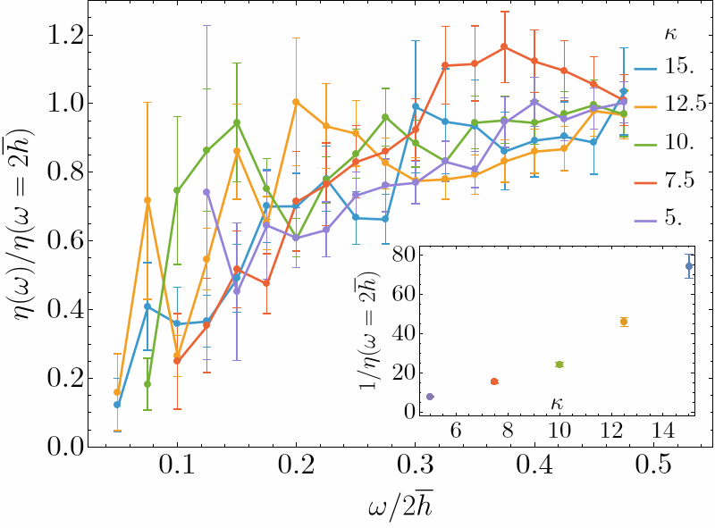
Figure 2: \(\eta(\omega)\), defined in Eq. (14 ),for \(\mathcal{D}=2\)-dimensional pseudospin model as a function of\(\omega\) for various disorders. The parameters and system sizes arethe same as in , apartfrom \(\lambda\) used to tune \(\kappa\). For each curve in the mainpanel, \(\omega\) and \(\eta(\omega)\) are normalized to, respectively,\(2\overline{h}\) and \(\eta(\omega=2\overline{h})\) for the given \(\kappa\) value.The inset shows the evolution of \(1/\eta(\omega=2\overline{h})\) withdisorder. The error bars correspond to statistical fluctuations ofboth the numerator and denominator in Eq. (14 )due to both the finite number of disorder realizations and the finitesize of each disorder realization. The number of disorder realizationsfor each \(\kappa\) varied from \(2\) to \(20\) to achieve comparableerror bars. In the main panel, only the points with the relative errorbelow 100% are presented, while the low-\(\omega\) data of poor qualityis left out..
1.0.2 Approximate expression for \(R_{ij}(\omega)\) at dissipative edges↩︎
The condition of low excitation frequency, \(\Omega_{ij}\ll\overline{h}\), is rather restrictive for possible disorder configurations of the effective two-spin Hamiltonian, Eq. (4 ). In Ref. [28] it is shown that two conditions have to be met: i) one of the two \(\xi\) fields—without loss of generality, let this be the field \(\xi_{1}\) on the first spin—has to be the largest scale, \(\left|\xi_{1}\right|\gg\left|\xi_{2}\right|,\,D_{12},\,h_{1\to2},\,h_{2\to1},\,\omega\), and ii) both local fields of the other spin have to be of the order of frequency: \(\left|\xi_{2}\right|,h_{1\to2}\apprle\omega\). Only under these conditions does the Hamiltoniani (4 ) posses an excitation with frequency \(\Omega_{12}=\omega\ll\overline{h}\). Under the same conditions, direct perturbation theory in powers of \(1/\left|\xi_{1}\right|\) yields the following result for the local superfluid response, Eq. (3 ): \[\begin{align} & \omega=\Omega_{12}\approx2\sqrt{\xi^{2}_{2}+\left(h_{2\to1}+D_{12}h_{1}/\left|\xi_{1}\right|\right)^{2}}, \tag{15}\\ & \frac{\text{Im}R_{12}(\omega)}{(2e)^{2}}\approx\left(D_{12}\frac{h_{1}}{\left|\xi_{1}\right|^{2}}\right)^{2}\tanh\frac{\Omega_{12}}{2T}\,\pi\delta\left(\omega-\Omega_{12}\right), \tag{16}\\ & \frac{R_{12}}{(2e)^{2}}\approx\frac{2D_{12}\,h_{1\to2}\,h_{2\to1}}{\Omega_{12}\,\left|\xi_{1}\right|}\tanh\frac{\Omega_{12}}{2T}. \tag{17} \end{align}\] Eq. (15 ) further implies the corresponding smallness of one of the two order parameter fields, \(h_{1\to2}\apprle\omega/2\ll\overline{h}\), explaining the connection of these excitations to the low-value tail of the order parameter. Subsequent averaging of Eq. (16 ) over disorder renders Eq. (11 ).
1.0.3 Statistical correlation between \(\left(\varphi_{i}-\varphi_{j}\right)^{2}\) and \(R_{ij}(\omega)\)↩︎
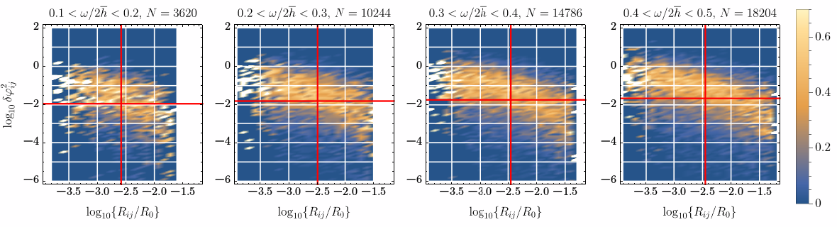
Figure 3: A series of color plots of the conditional probability \(P\left(\log_{10}\delta\varphi^{2}_{ij}\,|\,\log_{10}R_{ij}/R_{0};\,\omega_{1},\omega_{2}\right)\),defined in Eq. (18 ),for various frequency intervals \(\left[\omega_{1},\omega_{2}\right]\),specified on top of each plot in units of \(2\overline{h}\). To restorethe numerical e \(R_{0}=\left(2P_{0}\Delta_{0}\right)^{2}(2e)^{2}\Delta_{0}\).The red lines indicate the averages \(\overline{\log_{10}\delta\varphi^{2}_{ij}}\),\(\overline{\log_{10}R_{ij}/R_{0}}\) conditioned on the respectivefrequency interval, \(\omega_{1}<\Omega_{ij}<\omega_{2}\). The histogramis constructed from the dataset used in ,with the histogram bin sizes \(\delta\log_{10}R/R_{0}=0.1\), \(\delta\log_{10}\delta\varphi^{2}_{ij}=0.1\).The number of edges \(N\) contributing to each histogram is specifiedat the top of the respective plot. The irregularity of the plot onboth sides of the \(\log_{10}R_{ij}/R_{0}\) range is a finite sizeeffect due to small marginal probability \(P(\log_{10}R_{ij}/R_{0}|\omega_{1},\omega_{2})\)..
In this section, we review the correlations between the local superfluid response of a given edge \(\text{Re}R_{ij}(\omega=0)\), studied in Ref. [25] and denoted here \(R_{ij}\) for brevity, and the superconducting phase difference on the same edge. We focus our analysis on the edges that have sufficiently low excitation frequency to contribute to \(\text{Re}\sigma\) and thus influence its temperature dependence. To this end, visualizes the following conditional probability density \[\begin{align} & P\left(\psi\,|\,\rho;\,\omega_{1},\omega_{2}\right):=\nonumber \\ & \left.\overline{\delta\left(\log_{10}\delta\varphi^{2}_{ij}-\psi\right)\delta\left(\log_{10}R_{ij}/R_{0}-\rho\right)}_{\omega_{1}<\Omega_{ij}<\omega_{2}}\right/\nonumber \\ & \overline{\delta\left(\log_{10}R_{ij}/R_{0}-\rho\right)}_{\omega_{1}<\Omega_{ij}<\omega_{2}}. \label{eq:phase-conditional-probability-expression} \end{align}\tag{18}\] Here, \(R_{0}=\left(2P_{0}\Delta_{0}\right)^{2}(2e)^{2}\Delta_{0}\), \(\Omega_{ij}\) is the lowest excitation frequency of edge \(ij\) [see Eq. (9 )], the subscript means that only the edges satisfying \(\omega_{1}<\Omega_{ij}<\omega_{2}\)—and thus contributing to \(\text{Re}\sigma\) in the same frequency range—are used in the averaging, and \(\delta\varphi^{2}_{ij}\) is the normalized squared phase difference, \(\delta\varphi^{2}_{ij}=\mathcal{D}\left(\frac{\varphi_{i}-\varphi_{j}}{\overline{\nabla\varphi}}\right)^{2}\left/\overline{\left(\boldsymbol{r}_{i}-\boldsymbol{r}_{j}\right)^{2}}\right..\)
reveals the main qualitative features of the joint statistics of \(R_{ij}\) and \(\delta\varphi^{2}_{ij}\) for the dissipative edges: i) The marginal distribution of the logarithm of \(\delta\varphi^{2}_{ij}\), \(P\left(\psi|\omega_{1},\omega_{2}\right)=\intop^{\infty}_{-\infty}d\rho\,P\left(\psi|\rho,\omega_{1},\omega_{2}\right)\), is broad, with the values of \(\delta\varphi^{2}_{ij}\) distributed across multiple decades. This creates difficulties for the numerical analysis and, in particular, explains the strong statistical fluctuations observed in . ii) \(R_{ij}\) and \(\delta\varphi^{2}_{ij}\) are substantially anti-correlated, with larger \(R_{ij}\) leading to smaller \(\delta\varphi^{2}_{ij}\). iii) These correlations are only weakly sensitive to the frequency interval.
These features are essential for understanding the correct temperature dependence of the dissipative conductivity \(\text{Re}\sigma\). Indeed, as one increases the temperature starting from \(T=0\), the change in \(\text{Re}\sigma\) originates from both \(\text{Im}R_{ij}\) and \(\left(\varphi_{i}-\varphi_{j}\right)^{2}\), according to Eq. (7 ). The first of these two factors is correctly captured by the approximate Eq. (8 ). On the other hand, the temperature effect of \(\left(\varphi_{i}-\varphi_{j}\right)^{2}\) is hard to analyze numerically, as it requires solving the \(\omega=0\) NM for every \(T\), whereas all NM data in this work correspond to \(T=0\) and have already required substantial computational time. However, suggests that the temperature shift of \(\left(\varphi_{i}-\varphi_{j}\right)^{2}\) for the low-frequency edges can be inferred from that of \(R_{ij}\). According to Eq. (17 ), the main temperature dependence of both \(R_{ij}\) and \(\overline{\text{Im}R_{ij}(\omega)}\) is set by \(\Omega_{ij}\) via the common \(\tanh\frac{\omega}{2T}\) factor, whereas the typical temperature scale for the change of \(\Omega_{ij}\) and the \(h\) fields is \(\overline{h}\), which is assumed to be much higher than \(\omega\). Therefore, one expects \(R_{ij}\) to diminish strongly with \(T\) for the same low-frequency edges that contribute to dissipation. This conclusion is then transferred to \(\delta\varphi^{2}_{ij}\) by its anti-correlation with \(R_{ij}\), implying additional temperature dependence of \(\text{Re}\sigma\) that is not captured by Eq. (8 ). Ref. [28] conducts further empirical analysis of these correlations, which are argued to only alter the quantitative shape of the temperature dependence, while preserving the qualitative behavior shown in . A more detailed study of the temperature dependence of \(\text{Re}\sigma\) is a subject of future work.
References↩︎
In terms of original electronic operators: \(S_{j}=c_{j,\downarrow}c_{j,\uparrow}\), \(S^{+}_{j}=c^{+}_{j,\uparrow}c^{+}_{j,\downarrow}\), \(S^{z}_{j}=c^{+}_{j,\uparrow}c_{j,\uparrow}+c^{+}_{j,\downarrow}c_{j,\downarrow}-\frac{1}{2}\).↩︎
At finite \(\omega>0\), Eq. (6 ) also contains the nonlocal contributions from the phase differences on edges \(e\) other than \(\left\langle ij\right\rangle\), these terms can be naively estimated as \((\omega/\Delta_{0})^{2d}\), where \(d\) is the distance between \(e\) and \(\left\langle ij\right\rangle\) on the graph, see [25].↩︎
The use of the 2D geometry instead of the 3D one is a technical compromise to achieve convergence of disorder averages. The qualitative results of the analysis are expected to hold both in two and three dimensions since the relevant dissipative processes are inherently microscopic.↩︎
The model parameters for the data in Fig. , left were carefully chosen to maximize \(m_{\text{tree}}\) while still being within the range of applicability of the employed numerical methods, as detailed in Ref. [28].↩︎