Computing Evolutionarily Stable Strategies in Multiplayer Games
November 25, 2025
Abstract
We present an algorithm for computing all evolutionarily stable strategies in nondegenerate normal-form games with three or more players.
1 Introduction↩︎
While Nash equilibrium has emerged as the standard solution concept in game theory, it is often criticized as being too weak: often games contain multiple Nash equilibria (sometimes even infinitely many), and we want to select one that satisfies other natural properties. For example, one popular concept that refines Nash equilibrium is evolutionarily stable strategy (ESS). A mixed strategy in a two-player symmetric game is an evolutionarily stable strategy if it is robust to being overtaken by a mutation strategy. Formally, mixed strategy \(\mathbf{x}^*\) is an ESS if for every mixed strategy \(\mathbf{x}\) that differs from \(\mathbf{x}^*\), there exists \(\epsilon_0 = \epsilon_0(\mathbf{x}) > 0\) such that, for all \(\epsilon \in (0,\epsilon_0)\), \[(1-\epsilon)u_1(\mathbf{x},\mathbf{x}^*) + \epsilon u_1(\mathbf{x},\mathbf{x}) < (1-\epsilon)u_1(\mathbf{x}^*,\mathbf{x}^*)+\epsilon u_1(\mathbf{x}^*,\mathbf{x}).\] From a biological perspective, we can interpret \(\mathbf{x}^*\) as a distribution among “normal” individuals within a population, and consider a mutation that makes use of strategy \(\mathbf{x}\), assuming that the proportion of the mutation in the population is \(\epsilon\). In an ESS, the expected payoff of the mutation is smaller than the expected payoff of a normal individual, and hence the proportion of mutations will decrease and eventually disappear over time, with the composition of the population returning to being mostly \(\mathbf{x}^*\). An ESS is therefore a mixed strategy of the column player that is immune to being overtaken by mutations. ESS was initially proposed by mathematical biologists motivated by applications such as population dynamics (e.g., maintaining robustness to mutations within a population of humans or animals) [1], [2]. A common example game is the 2x2 game where strategies correspond to an “aggressive” Hawk or a “peaceful” Dove strategy. A paper has recently proposed a similar game in which an aggressive malignant cell competes with a passive normal cell for biological energy, which has applications to cancer eradication [3].
While Nash equilibrium is defined for general multiplayer games, ESS is traditionally studied in the context of symmetric two-player games. ESS is a refinement of Nash equilibrium. In particular, if \(\mathbf{x}^*\) is an ESS, then \((\mathbf{x}^*,\mathbf{x}^*)\) (i.e., the strategy profile where both players play \(\mathbf{x}^*\)) is a (symmetric) Nash equilibrium [4]. Of course the converse is not necessarily true (not every symmetric Nash equilibrium is an ESS), or else ESS would be a trivial refinement. In fact, ESS is not guaranteed to exist in games with more than two pure strategies per player (while Nash equilibrium is guaranteed to exist in all finite games). For example, while rock-paper-scissors has a mixed strategy Nash equilibrium (which puts equal weight on all three actions), it has no ESS [4] (that work considers a version where payoffs are 1 for a victory, 0 for loss, and \(\frac{2}{3}\) for a tie).
There exists a polynomial-time algorithm for computing Nash equilibrium (NE) in two-player zero-sum games, while for two-player non-zero-sum and multiplayer games computing an NE is PPAD-complete and it is widely conjectured that no efficient (polynomial-time) algorithm exists. However, several algorithms have been devised that perform well in practice. The problem of deciding whether a game has an ESS was shown to be both NP-hard and CO-NP hard and also to be contained in \(\Sigma ^P _2\) (the class of decision problems that can be solved in nondeterministic polynomial time given access to an NP oracle) [5]. Subsequently it was shown that the exact complexity of this problem is that it is \(\Sigma ^P _2\)-complete [6], and even more challenging for more than two players [7]. Note that this result is for determining whether an ESS exists (as discussed above there exist games which have no ESS), not for the complexity of computing an ESS in games for which one exists. Thus, computing an ESS is significantly more difficult than computing an NE, which is not surprising since it is a refinement. Several approaches have been proposed for computing ESS in two-player games [8]–[12]. However, we are not aware of approaches for computing ESS in games with 3+ players.
Many evolutionary models of tumor ecology involve frequency-dependent interactions among three or more cancer cell phenotypes (e.g., [13]–[16]). These systems are naturally formulated as symmetric \(n\)-player games, and ESS provides a biologically meaningful stability concept. Motivated by this, we develop an algorithm for computing evolutionarily stable strategies in multiplayer symmetric normal-form games. Evolutionarily stable strategies in multiplayer symmetric games have been studied in the evolutionary game theory literature, beginning with early work by Palm [17] and subsequently developed by Broom, Cannings, and Vickers [18], among others.
A normal-form game consists of a finite set of players \(N = \{1,\ldots,n\}\), a finite set of pure strategies \(S_i\) for each player \(i\), and a real-valued utility for each player for each strategy vector (aka strategy profile), \(u_i : \times_i S_i \rightarrow \mathbb{R}\). In a symmetric normal-form game, all strategy spaces \(S_i\) are equal and the utility functions satisfy the following symmetry condition: for every player \(i \in N\), pure strategy profile \((s_1,\ldots,s_n) \in S^n\), and permutation \(\pi\) of the players, \[u_i(s_1,\ldots,s_n) = u_{\pi(i)}(s_{\pi(1)},\ldots,s_{\pi(n)}).\] This allows us to remove the player index of the utility function and just write \(u(s_1,\ldots,s_n),\) where it is implied that the utility is for player 1 (we can simply permute the players to obtain the utilities of the other players). We will still write \(u_i\) for notational convenience, but note that only a single utility function must be specified which will apply to all players.
Let \(\Sigma_i\) denote the set of mixed strategies of player \(i\) (probability distributions over elements of \(S_i\)). If players follow mixed strategy profile \(\mathbf{x} = (\mathbf{x}^{(1)},\ldots,\mathbf{x}^{(n)}),\) where \(\mathbf{x}^{(i)} \in \Sigma_i\), the expected payoff to player \(i\) is \[u_i(\mathbf{x}^{(1)},\ldots,\mathbf{x}^{(n)}) = \sum_{s_1,\ldots,s_n \in S} x^{(1)}_{s_1} \cdots x^{(n)}_{s_n}u_i(s_1,\ldots,s_n).\] We write \(u_i(\mathbf{x}) = u_i(\mathbf{x}^{(i)},\mathbf{x}^{(-i)})\), where \(\mathbf{x}^{(-i)}\) denotes the vector of strategies of all players except \(i\). If all players follow the same mixed strategy \(\mathbf{x}\), then for all players \(i\) we have \[u_i(\mathbf{x}) = u_i(\mathbf{x},\ldots,\mathbf{x}) = \sum_{s_1,\ldots,s_n \in S} x_{s_1} \cdots x_{s_n} u_i(s_1,\ldots,s_n).\]
Definition 1. A mixed strategy profile \(\mathbf{x}^*\) is a Nash equilibrium if for each player \(i \in N\) and for each mixed strategy \(\mathbf{x}^{(i)} \in \Sigma_i\): \(u_i(\mathbf{x}^{*(i)},\mathbf{x}^{*(-i)}) \geq u_i(\mathbf{x}^{(i)},\mathbf{x}^{*(-i)}).\)
Definition 2. A mixed strategy profile \(\mathbf{x}^*\) in a symmetric normal-form game is a symmetric Nash equilibrium if it is a Nash equilibrium and: \(\mathbf{x}^{*(1)} = \mathbf{x}^{*(2)} = \cdots = \mathbf{x}^{*(n)}.\)
Definition 3 (Broom, Cannings, and Vickers [18]). A mixed strategy \(\mathbf{x}^* \in \Sigma_1\) is evolutionarily stable* in a symmetric normal-form game if for each mixed strategy \(\mathbf{x} \neq \mathbf{x}^*\) there exists an integer \(r \in \{0,\ldots,n-1\}\) such that \[u_1(\mathbf{x}^*,\underbrace{\mathbf{x},\ldots,\mathbf{x}}_{r}, \underbrace{\mathbf{x}^*,\ldots,\mathbf{x}^*}_{n-1-r}) > u_1(\underbrace{\mathbf{x},\ldots,\mathbf{x}}_{r+1}, \underbrace{\mathbf{x}^*,\ldots,\mathbf{x}^*}_{n-1-r}),\] and for every \(j<r\), \[u_1(\mathbf{x}^*,\underbrace{\mathbf{x},\ldots,\mathbf{x}}_{j}, \underbrace{\mathbf{x}^*,\ldots,\mathbf{x}^*}_{n-1-j}) = u_1(\underbrace{\mathbf{x},\ldots,\mathbf{x}}_{j+1}, \underbrace{\mathbf{x}^*,\ldots,\mathbf{x}^*}_{n-1-j}).\]*
For the special case of \(n = 3\) players, a mixed strategy \(\mathbf{x}^*\) is evolutionarily stable if for every mixed strategy \(\mathbf{x} \neq \mathbf{x}^*\) exactly one of the following conditions holds:
\(u_1(\mathbf{x}^*,\mathbf{x}^*,\mathbf{x}^*) > u_1(\mathbf{x},\mathbf{x}^*,\mathbf{x}^*)\),
\(u_1(\mathbf{x}^*,\mathbf{x}^*,\mathbf{x}^*) = u_1(\mathbf{x},\mathbf{x}^*,\mathbf{x}^*)\) and \(u_1(\mathbf{x}^*,\mathbf{x},\mathbf{x}^*) > u_1(\mathbf{x},\mathbf{x},\mathbf{x}^*)\),
\(u_1(\mathbf{x}^*,\mathbf{x}^*,\mathbf{x}^*) = u_1(\mathbf{x},\mathbf{x}^*,\mathbf{x}^*)\), \(u_1(\mathbf{x}^*,\mathbf{x},\mathbf{x}^*) = u_1(\mathbf{x},\mathbf{x},\mathbf{x}^*)\), and \(u_1(\mathbf{x}^*,\mathbf{x},\mathbf{x}) > u_1(\mathbf{x},\mathbf{x},\mathbf{x})\).
It has been proven that every symmetric normal-form game has at least one symmetric Nash equilibrium [19]. It is clear from Definition 3 that every evolutionarily stable strategy (ESS) in a symmetric normal-form game must be a symmetric Nash equilibrium (SNE). Following standard practice in the equilibrium computation literature [20]–[22], we restrict attention to nondegenerate symmetric games, for which each support admits at most one symmetric Nash equilibrium.
2 Algorithm↩︎
In this section we present our main algorithm for computing all ESSs in nondegenerate symmetric normal-form games. We present our algorithm just for the three-player case and discuss how it can be extended to \(n\) players. The algorithm works by enumerating supports, and for each support computing a symmetric Nash equilibrium (SNE) if it exists (recall that under the nondegeneracy assumption there is at most one SNE for each support). If an SNE \(\mathbf{x}\) is found, we then run a procedure to test whether \(\mathbf{x}\) is an ESS. The procedures for computing an SNE given a support, and for testing whether an SNE is an ESS, each involve solving a nonconvex quadratically-constrained program. Note that our algorithm finds all ESSs since it enumerates over all supports; if our goal was just to find one ESS we could halt the algorithm as soon as one ESS is found. If the game does not contain an ESS then the algorithm will correctly output that no ESS exists. If the game is in fact degenerate then our algorithm may fail to find all ESSs, but will never output a non-ESS.
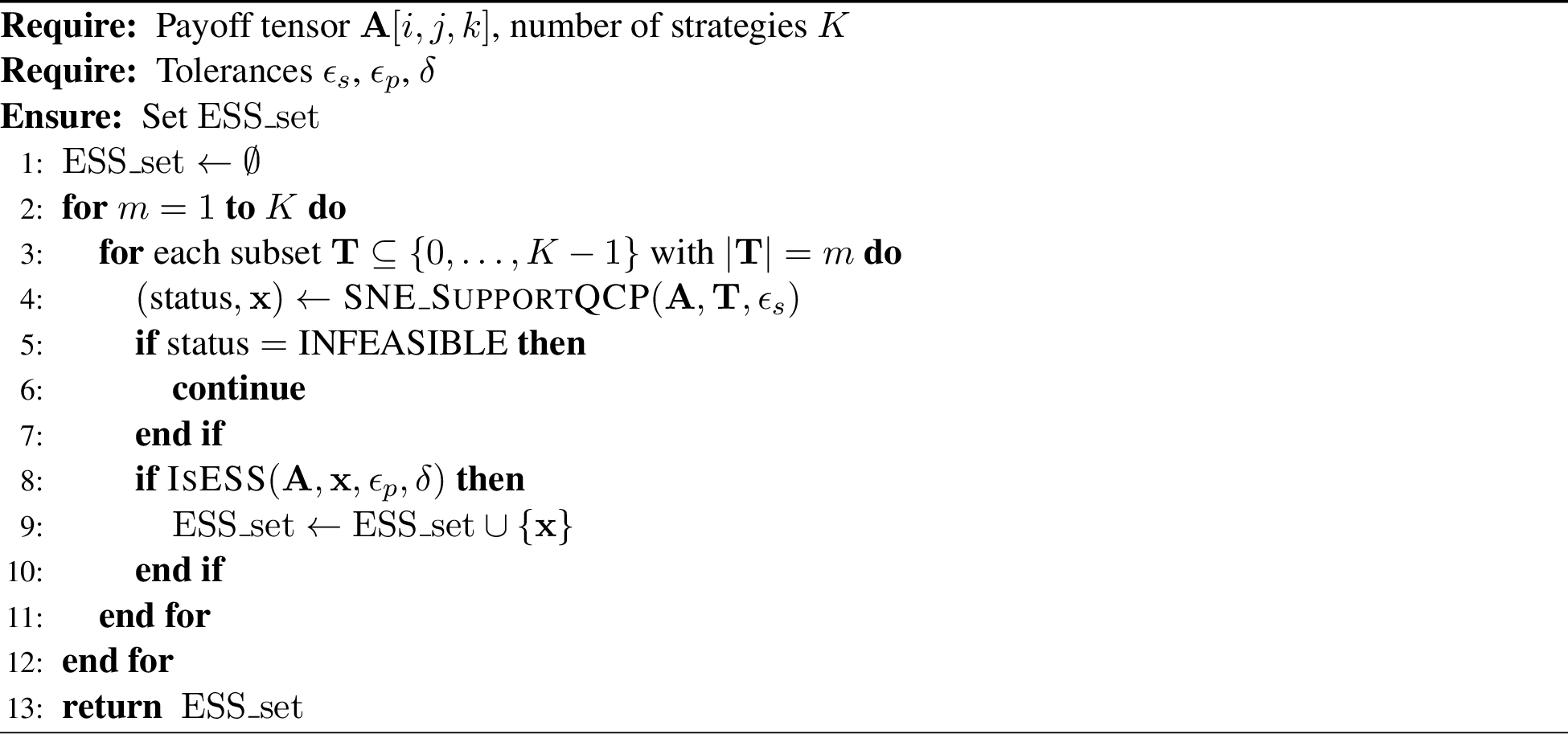
Algorithm 1 presents pseudocode for the main algorithm. The input is a payoff tensor \(\mathbf{A}\), where \(A[i,j,k]\) is the payoff to player 1 when player 1 plays pure strategy \(i,\) player 2 plays pure strategy \(j\), and player 3 plays pure strategy \(k.\) The algorithm also uses several numerical parameters whose values are given in Table 1. The output of the algorithm is the (possibly empty) set of ESSs. The outer loop iterates over all supports \(\mathbf{T}\) in increasing order of their dimension. For each support, we test whether the game has an SNE with that support using Algorithm 2. If there exists an SNE \(\mathbf{x}\) for support \(\mathbf{T}\), we then run Algorithm 3 to test whether or not \(\mathbf{x}\) is an ESS, and if so we add it to our list of ESSs that is output.
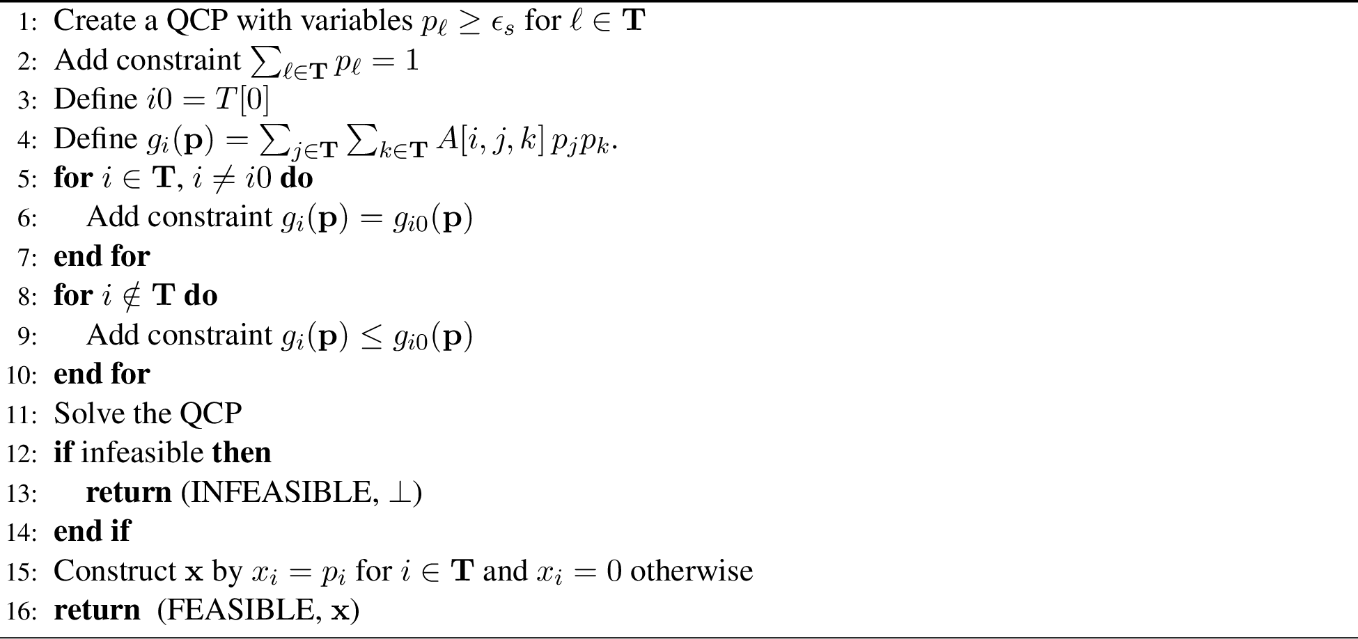
Algorithm 2 tests whether the game has an SNE with given support \(\mathbf{T}\) by creating and solving a quadratically-constrained feasibility program (QCP). The variables \(p_\ell\) represent the non-negative strategy probabilities over the elements of \(\mathbf{T}\). We define \(g_i(\mathbf{p})\) to be the expected payoff of playing pure strategy \(i\) when the opposing players play \(\mathbf{p}.\) Note that \(g_i(\mathbf{p})\) is quadratic since it contains products of variables \(p_j p_k.\) For each \(i \in \mathbf{T},\) we add the constraint \(g_i(\mathbf{p}) = g_{i0}(\mathbf{p})\), and for each \(i \notin \mathbf{T}\), we add the constraint \(g_i(\mathbf{p}) \le g_{i0}(\mathbf{p})\). This ensures that the player is indifferent between all pure strategies in the support and cannot profitably deviate to a strategy outside the support, which is the definition of Nash equilibrium.
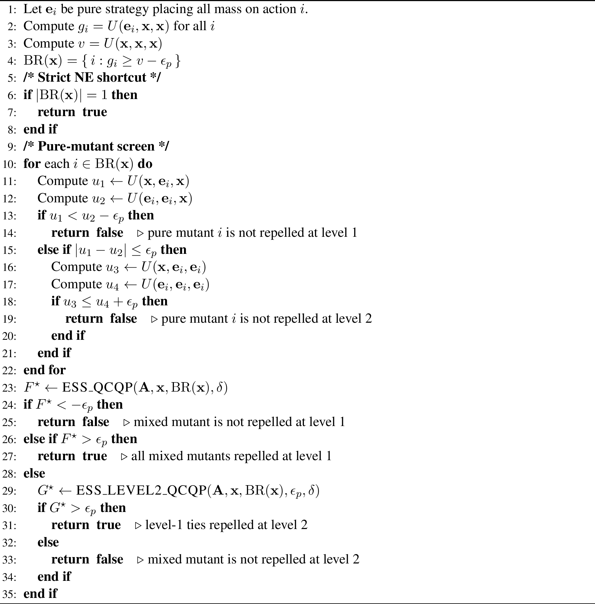
Given SNE \(\mathbf{x}\), Algorithm 3 determines whether it is an ESS. The multilinear payoff to player 1 is defined as \[U(\mathbf{a},\mathbf{b},\mathbf{c}) = \sum_{i,j,k} A[i,j,k]\, a_i b_j c_k.\] We first check whether \(\mathbf{x}\) is a strict Nash equilibrium. It is well known that in symmetric games any strict SNE is an ESS [1], [2], [23]. Moreover, among symmetric Nash equilibria, strictness is equivalent to being a pure strategy whose chosen action is the unique best response to itself [2], [23]. Consequently, whenever \(\mathbf{x}\) is pure and satisfies \(|BR(\mathbf{x})|=1\), we may immediately conclude that \(\mathbf{x}\) is an ESS. Note that \(|BR(\mathbf{x})|=1\) implies that \(\mathbf{x}\) is pure, so we can simplify this procedure to just check if \(|BR(\mathbf{x})|=1.\) We next test whether a pure mutant can invade \(\mathbf{x}\) by iterating over all pure strategies \(i \in \mathrm{BR}(\mathbf{x})\). For each such \(i\), we first compare \(U(\mathbf{x},\mathbf{e}_i,\mathbf{x})\) and \(U(\mathbf{e}_i,\mathbf{e}_i,\mathbf{x})\). If the two quantities are equal up to numerical tolerance, then we apply the second-level comparison \(U(\mathbf{x},\mathbf{e}_i,\mathbf{e}_i)\) versus \(U(\mathbf{e}_i,\mathbf{e}_i,\mathbf{e}_i)\), as required by Definition 3. After applying these efficient tests, we apply Algorithms 4 and 5 to determine whether \(\mathbf{x}\) can be invaded by any mixed mutant.
Algorithm 4 performs the first-level mixed-mutant test. The variables \(y_i\) represent the non-negative strategy probabilities over the elements of \(\mathrm{BR}(\mathbf{x})\). Let \(\mathbf{y}\) denote the extension of this vector to a \(K\)-dimensional strategy by setting entries not in \(\mathrm{BR}(\mathbf{x})\) to zero. The algorithm minimizes \[F(\mathbf{y}) = U(\mathbf{x},\mathbf{y},\mathbf{x}) - U(\mathbf{y},\mathbf{y},\mathbf{x}).\] If the minimum value is positive, then every mixed mutant is repelled at the first level of Definition 3. If it is negative, then some mixed mutant invades at the first level. If the value is approximately zero, then Algorithm 5 applies the second-level comparison by minimizing \[G(\mathbf{y}) = U(\mathbf{x},\mathbf{y},\mathbf{y}) - U(\mathbf{y},\mathbf{y},\mathbf{y})\] over mutants for which \(F(\mathbf{y})\) is approximately zero. Numerically, we say that \(\mathbf{y} \neq \mathbf{x}\) when \(\|\mathbf{y}-\mathbf{x}\|_2 \ge \delta\).
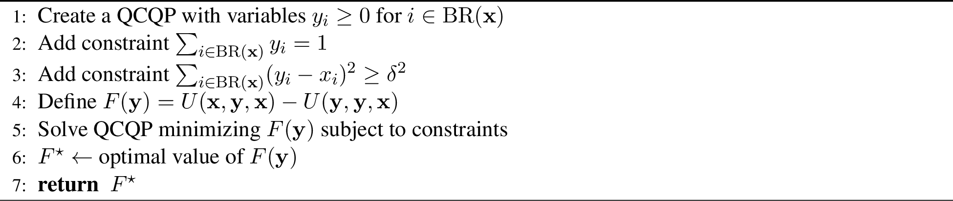
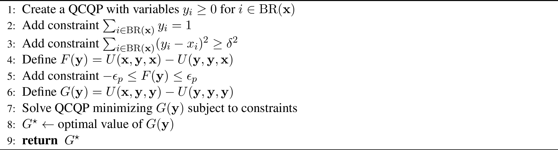
The QCP in Algorithm 2 and the QCQP in Algorithm 4 have nonconvex quadratic constraints, and Algorithm 4 also has a nonconvex quadratic objective. Algorithm 5 introduces the second-level mixed-mutant test. For the 3-player case, the objective \[G(\mathbf{y}) = U(\mathbf{x},\mathbf{y},\mathbf{y}) - U(\mathbf{y},\mathbf{y},\mathbf{y})\] contains cubic terms in \(\mathbf{y}\). We reformulate this problem as a QCQP by introducing auxiliary variables for products of the components of \(\mathbf{y}\), and solve all of these programs using Gurobi’s nonconvex quadratic solver [24]. We will use Gurobi’s default feasibility tolerance of \(10^{-6}\) (meaning that it is possible that constraints are violated by up to \(10^{-6}\)). This will influence our selection of the numerical parameters in the algorithm, depicted in Table 1. The parameter \(\epsilon_s\) is used in Algorithm 2 to ensure that pure strategies in the support are played with nonzero probability. Note that our value of \(\epsilon_s = 10^{-4}\) is larger than Gurobi’s feasibility tolerance. The parameter \(\epsilon_p\) is used in Algorithm 3 to compare payoffs. While it is not mentioned in the pseudocode, we recompute \(F^*\) from the optimal \(\mathbf{y}\) rather than using the optimal value returned by Gurobi which may have small numerical imprecision. The value of \(\epsilon_p = 10^{-5}\) is again larger than the feasibility tolerance. The final parameter \(\delta = 10^{-2}\) is used in Algorithm 4 to ensure that \(\mathbf{y}\) differs from \(\mathbf{x}\). Note that \(\delta^2 = 10^{-4},\) which is significantly larger than the feasibility tolerance as well as \(\epsilon_p\), but still sufficiently small to reasonably approximate an infinitesimal neighborhood around \(\mathbf{x}.\)
| Parameter | Value | ||||
|---|---|---|---|---|---|
| \(\epsilon_s\) | \(10^{-4}\) | ||||
| \(\epsilon_p\) | \(10^{-5}\) | ||||
| \(\delta\) | \(10^{-2}\) |
While we have presented the algorithm just for the 3-player case, it extends naturally to \(n > 3\) players. The main difference is that \(g_i(\mathbf{p})\) in Algorithm 2 will involve a product of \(n-1\) variables instead of 2. We can convert these expressions to equivalent expressions that are quadratic by introducing auxiliary variables. For example for \(n = 4\), we can set \(p_{12} = p_1 p_2\), \(p_{123} = p_{12}p_3\), etc. Thus the programs will have more variables, but they will remain quadratic and can be solved as a QCP with Gurobi’s nonconvex quadratic solver. The first-level mixed-mutant test remains quadratic for \(n>3\) players. However, the full ESS test requires additional higher-level comparisons analogous to Algorithm 5. These higher-level tests involve higher-degree polynomial objectives, which can be reformulated as QCQPs using auxiliary product variables. For example, the first-level mixed-mutant test minimizes \[F(y)=U(x,y,x,\ldots,x)-U(y,y,x,\ldots,x).\] Since the first term is linear in \(y\) and the second term is quadratic in \(y\), this objective is quadratic in \(y\). Also note that the number of supports enumerated over in Algorithm 1 remains \(2^K - 1\) independently of the number of players \(n.\)
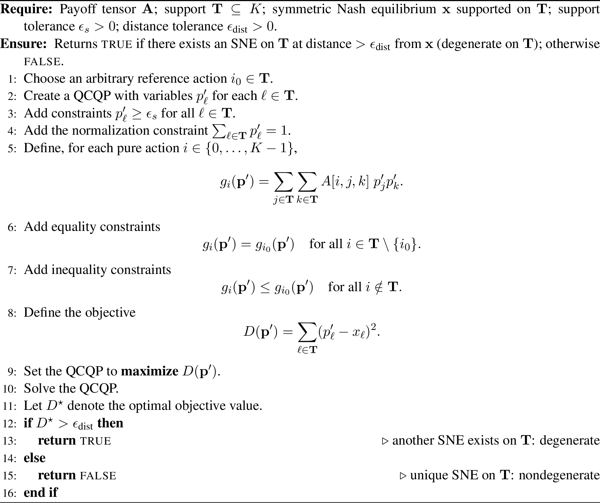
We also note that while the algorithm is specifically designed for nondegenerate games (for which there is at most one SNE with a given support), the algorithm can still be applied to degenerate games as well. The set of ESSs found is guaranteed to be a subset of the full set of ESSs, but the algorithm may fail to find all of the ESSs. The question still remains of how to determine whether a given game is degenerate. Note that for games with uniform random payoffs the set of games that are degenerate has measure zero. So any degenerate game could be converted to a “similar” nondegenerate game by adding small perturbations to the payoffs. Otherwise, it is not trivial to determine whether a game is degenerate and we must apply an additional procedure. One such procedure is provided in Algorithm 6. After computing an SNE \(\mathbf{x}\) on support \(\mathbf{T}\) in Algorithm 1, we can then solve a QCQP that finds the SNE on support \(\mathbf{T}\) with largest Euclidean distance from \(\mathbf{x}.\) Let \(D^\star\) denote the optimal objective value. If \(D^\star > \epsilon_{\text{dist}}\), then we conclude that there exists another SNE distinct from \(\mathbf{x}\) on support \(\mathbf{T}\), which implies that the game is degenerate. If \(D^\star \leq \epsilon_{\text{dist}}\) for all supports \(\mathbf{T},\) then we conclude that the game is nondegenerate. We can set \(\epsilon_{\text{dist}} = 10^{-8}\), which is several orders of magnitude larger than the squared distance induced by feasibility tolerance, while still providing a practical numerical threshold for distinguishing distinct SNE. If we include this procedure, then we will be solving a QCP and QCQP for each support; but we will know for sure whether we are outputting all ESSs.
3 Experiments↩︎
Our first set of experiments is on a set of example games given in Appendix 5. The full sets of SNE and ESSs for these games are summarized in Table 2. Note that several of these games are degenerate in the sense that certain supports contain a continuum of symmetric Nash equilibria. For Games 1, 3, 4, 6, 7, and 8, the algorithm correctly found all SNE and ESSs. For Game 2, the algorithm found SNE (1,0), (0,1), and \((0.9999,\num{1e-4}).\) This game is degenerate on the support \(\{0,1\},\) and the algorithm is only expected to find one representative SNE on such a support; it also correctly classified that no ESSs exist. For Game 5 the algorithm found SNE (1,0,0) and \((0,0.9999,\num{1e-4}).\) The game is degenerate on the support \(\{1,2\},\) so the algorithm does not return all SNE on that face, but it correctly identified the unique ESS. Game 6 represents frequency-dependent competition among three tumor phenotypes—Proliferators, Producers, and Invasives—where each cell’s payoff equals the sum of its pairwise interactions with two neighbors. Proliferators and Invasives each receive the highest payoff when interacting with their own type, while Producers confer no competitive advantage.
| Game | \(K\) | SNE | ESS |
|---|---|---|---|
| 1 | 2 | \(\{(0,1),\; (1/2,1/2)\}\) | \(\{(0,1),\; (1/2,1/2)\}\) |
| 2 | 2 | All mixed strategies | \(\varnothing\) |
| 3 | 2 | \(\{(1,0),\; (0,1)\}\) | \(\{(1,0)\}\) |
| 4 | 3 | \(\{(1/3,\,1/3,\,1/3)\}\) | \(\varnothing\) |
| 5 | 3 | \(\{(1,0,0)\} \;\cup\; \{(0,x,y): x,y \ge 0,\;x+y=1\}\) | \(\{(1,0,0)\}\) |
| 6 | 3 | \(\{(1,0,0),\;(0,1,0),\;(0,0,1),\;(0.5, 0, 0.5)\}\) | \(\{(1,0,0),\;(0,0,1)\}\) |
| 7 | 3 | \(\{(1,0,0),\;(0,1,0),\;(0,0,1),\) \((3/7,\,4/7,\,0),\;(0,\,1/3,\,2/3),\;(0.2,\,0.4,\,0.4)\}\) | \(\{(1,0,0),\;(0,1,0)\}\) |
| 8 | 3 | \(\{(0.4311484,\,0.3760157,\,0.1928359)\}\) | \(\{(0.4311484,\,0.3760157,\,0.1928359)\}\) |
For our next experiments we ran our algorithm on three-player symmetric normal-form games with all payoff entries uniformly random on [-1,1]. We generated and solved 100 games for each number of pure strategies \(K\) from 3 to 8. These games are nondegenerate since the set of degenerate games has Lebesgue measure zero. We used the nonconvex quadratic solver from Gurobi version 13.0.0, which guarantees global optimality [24], with Java version 14.0.2. We used an Intel Core i7-1065G7 processor with base clock speed of 1.30 GHz (and maximum turbo boost speed of up to 3.9 GHz) with 16 GB of RAM under 64-bit Windows 11 (8 logical cores/threads). We used the numerical parameter values given in Table 1.
The runtimes from the experiments are given in Table 3. For each \(K\) we report the total runtime of Algorithm 1 to find all ESSs, as well as the runtime until the first ESS is found. If no ESSs are found, then we report the time to find the first ESS as the total time of Algorithm 1. For both the total and first runtimes we report the mean with 95% confidence intervals as well as the median. The results indicate that the algorithm is able to find all ESSs quite quickly in these games. For the biggest games \(K = 8\) the mean runtime to find all ESSs is 13.8159 seconds, and the mean runtime to find one ESS is 0.7645 seconds. For \(K =\) 3–5, all ESSs are found in a fraction of a second. Since the games are nondegenerate, we know that the algorithm finds all ESSs in each game.
| \(K\) | Mean Total (\(\pm\) 95% CI) | Median Total | Mean First (\(\pm\) 95% CI) | Median First |
|---|---|---|---|---|
| 3 | 0.0169 \(\pm\) 0.0055 | 0.0115 | 0.0058 \(\pm\) 0.0017 | 0.0030 |
| 4 | 0.1147 \(\pm\) 0.0232 | 0.0875 | 0.0186 \(\pm\) 0.0102 | 0.0050 |
| 5 | 0.3120 \(\pm\) 0.0261 | 0.2985 | 0.0339 \(\pm\) 0.0190 | 0.0050 |
| 6 | 0.9425 \(\pm\) 0.0817 | 0.8560 | 0.0345 \(\pm\) 0.0268 | 0.0030 |
| 7 | 4.4113 \(\pm\) 0.2795 | 4.5825 | 0.3080 \(\pm\) 0.2568 | 0.0040 |
| 8 | 12.9643 \(\pm\) 0.5866 | 12.6410 | 0.5825 \(\pm\) 0.5247 | 0.0040 |
Table 4 provides further insight by showing the number of ESSs found for each \(K\) (aggregated over the 100 sampled games). While a small number of games had no ESS, the majority of games had a moderate number of ESSs (1–3). Table 5 gives a breakdown of the number of ESSs found with each support size, again aggregated over the sampled games. A large number of the ESSs had support size of 1 or 2, which explains why the running times to find the first ESS were so low; however some games had ESSs with larger support sizes.
| \(K\) | 0 | 1 | 2 | 3 | 4 | 5 | 6 | 7 |
|---|---|---|---|---|---|---|---|---|
| 3 | 3 | 45 | 44 | 8 | 0 | 0 | 0 | 0 |
| 4 | 2 | 39 | 40 | 17 | 2 | 0 | 0 | 0 |
| 5 | 4 | 25 | 37 | 22 | 11 | 1 | 0 | 0 |
| 6 | 2 | 21 | 39 | 31 | 6 | 1 | 0 | 0 |
| 7 | 4 | 20 | 32 | 30 | 8 | 3 | 2 | 1 |
| 8 | 4 | 14 | 34 | 29 | 14 | 3 | 2 | 0 |
| \(K\) | \(s{=}1\) | \(s{=}2\) | \(s{=}3\) | \(s{=}4\) | \(s{=}5\) |
|---|---|---|---|---|---|
| 3 | 101 | 55 | 1 | 0 | 0 |
| 4 | 92 | 62 | 23 | 1 | 0 |
| 5 | 91 | 98 | 22 | 3 | 0 |
| 6 | 102 | 70 | 43 | 6 | 0 |
| 7 | 101 | 100 | 28 | 10 | 1 |
| 8 | 109 | 90 | 48 | 4 | 1 |
Table 6 provides a breakdown of the outcomes of the ESS test described in Algorithm 3. The failure columns indicate the stage at which candidate SNE are eliminated. Thus, \[\text{Total ESS} = \text{Total SNE} - \text{Pure-Fail-L1} - \text{Pure-Fail-L2} - \text{Mixed-Fail-L1} - \text{Mixed-Fail-L2}.\] The results show that the pure-mutant screen eliminates the majority of non-strict SNE. For example, when \(K=8\), the algorithm encounters 1375 SNE, of which 109 are immediately classified as ESS by the strict NE shortcut. Among the remaining 1266 non-strict SNE, the first-level pure-mutant test eliminates 1066 (and the second-level pure-mutant test eliminates one). Thus only 199 candidates require solving the mixed-mutant optimization problems, a reduction of 84.3% relative to testing all non-strict SNE by mixed-mutant optimization. In total, for \(K = 8\) these two procedures reduce the number of strategies for which the QCQP procedures of Algorithm 4 and 5 must be applied from 1375 to 199, which is a reduction of 85.5%. The second-level pure-mutant test is rarely decisive in these random games, while the second-level mixed-mutant test eliminates a small but nonzero number of candidates.
| \(K\) | Total SNE | Strict SNE | Pure-Fail-L1 | Pure-Fail-L2 | Mixed-Fail-L1 | Mixed-Fail-L2 | Total ESS |
|---|---|---|---|---|---|---|---|
| 3 | 249 | 101 | 91 | 0 | 1 | 0 | 157 |
| 4 | 341 | 92 | 148 | 0 | 8 | 7 | 178 |
| 5 | 588 | 91 | 352 | 0 | 16 | 6 | 214 |
| 6 | 763 | 102 | 508 | 0 | 30 | 4 | 221 |
| 7 | 1014 | 101 | 726 | 3 | 39 | 6 | 240 |
| 8 | 1375 | 109 | 1066 | 1 | 46 | 10 | 252 |
4 Conclusion↩︎
We introduced the first algorithm for computing evolutionarily stable strategies in nondegenerate symmetric multiplayer normal-form games. Our approach enumerates supports and determines, for each support, whether it contains a symmetric Nash equilibrium and whether that equilibrium is evolutionarily stable. The method combines two efficient preprocessing tests—the strict Nash equilibrium shortcut and a pure-mutant screen—with a final mixed-mutant quadratically-constrained quadratic program that certifies evolutionary stability. We also developed a procedure for testing whether a given game is degenerate; for degenerate games our algorithm is guaranteed to find a subset of the ESSs. Experiments on eight benchmark games and random games with up to eight strategies demonstrate that the algorithm is fast in practice and reliably finds all ESSs. The breakdown of algorithmic components shows that the preprocessing tests eliminate over 85% of mixed-mutant QCQP solves for \(K = 8\), highlighting the practical impact of these refinements. Our results provide the first scalable computational tool for studying evolutionary stability in multiplayer interactions, with potential applications to evolutionary game theory, behavioral ecology, and tumor ecology. Future work includes extending these techniques to structured populations, dynamic stability refinements, and incomplete-information evolutionary models.
While our algorithm is only guaranteed to find all ESSs in nondegenerate games, it is still guaranteed to find a subset of all ESSs if run on degenerate games. Thus, the algorithm may still be useful in practice even on degenerate games. Two of the eight example games considered are degenerate; on the first the algorithm correctly classified that no ESSs exist, and on the second the algorithm correctly found the unique ESS. Algorithm 6 provides a procedure for detecting whether a support admits multiple symmetric Nash equilibria. Future work can build on this idea by developing methods that more completely characterize the set of equilibria on degenerate supports. For example, after finding one symmetric Nash equilibrium \(x\), one can repeatedly solve optimization problems that search for additional equilibria that are maximally distant from those already found. Such an approach may be useful for identifying multiple representative equilibria on degenerate supports, although it cannot in general enumerate the full set of equilibria when that set forms a continuum, as several of the example games demonstrate.
While the presentation of our algorithm and our experiments were focused on 3-player games, our algorithm is straightforwardly applicable to games with \(n > 3\) players. As described in Section 2, the only difference is that the QCP for computing an SNE in Algorithm 2 will involve expressions that are degree-(\(n-1\)) polynomial of the variables instead of quadratic. We can convert this to a quadratic program by adding auxiliary variables, e.g., \(p_{12} = p_1 p_2\), \(p_{123} = p_{12}p_3.\) In general for support size \(s\) and \(n\) players, we will require \(O(s^{n-1})\) variables, which is \(O(K^{n-1})\) in the worst case where \(K\) is the number of pure strategies. So the number of variables is exponential in \(n\), but a polynomial in \(K\) (for fixed \(n\)). Note that the first-level mixed-mutant test remains quadratic for \(n > 3.\) However, the full ESS test requires additional higher-level mutant comparisons analogous to Algorithm 5, which can be reformulated as QCQPs using auxiliary product variables. The total number of supports enumerated over remains \(2^K - 1\) independently of \(n.\) By contrast, if we were iterating over all possible support combinations to find a Nash equilibrium in a game that is not necessarily symmetric, we would need to consider \((2^K-1)^n\) support profiles, which is exponential in both \(K\) and \(n.\)
While we presented several preprocessing procedures that are shown to significantly improve computational efficiency—the strict Nash equilibrium shortcut and pure-mutant screen—our algorithm’s efficiency can likely be further optimized significantly. A support-enumeration approach for computing a Nash equilibrium in \(n\)-player normal-form games (that are not necessarily symmetric) performs a recursive procedure of iteratively removing conditionally strictly dominated strategies before solving a feasibility program [25]. Perhaps this additional preprocessing procedure could be effective in reducing the number of supports considered and/or the size of the corresponding QCPs solved in our algorithm as well. With access to additional computational resources our algorithm could also benefit from parallel computation, most obviously by solving multiple QCPs or QCQPs simultaneously. We showed that for 3-player games with \(K = 8\) strategies per player our algorithm is able to run quickly on a laptop without any of these additional enhancements. It is promising that our algorithm can be easily applied to small and moderate-sized games already in its current form, even if the goal is to find all ESSs. For larger games that the algorithm is unable to solve, it is still possible that our algorithm can solve them if augmented by efficiency enhancements such as those described above.
5 Payoff Tensors for the Example Games↩︎
All games are symmetric 3–player. For each action \(i\), \(A[i,:,:]\) gives the focal player’s payoff when the co–players use \(j,k\).
5.0.0.1 Game 1 (two–strategy game with pure and mixed ESS)
\[A[0] = \begin{pmatrix} -3 & 0\\ 0 & -3 \end{pmatrix}, \qquad A[1] = \begin{pmatrix} 1 & -3\\ -3 & -1 \end{pmatrix}.\]
5.0.0.2 Game 2 (neutral two–strategy game)
\[A[0] = \begin{pmatrix} 1 & 0\\ 0 & 1 \end{pmatrix}, \qquad A[1] = \begin{pmatrix} 1 & 0\\ 0 & 1 \end{pmatrix}.\]
5.0.0.3 Game 3 (strict dominance of strategy 0)
\[A[0] = \begin{pmatrix} 2 & 0\\ 0 & 0 \end{pmatrix}, \qquad A[1] = \begin{pmatrix} 0 & 0\\ 0 & 0 \end{pmatrix}.\]
5.0.0.4 Game 4 (three–strategy rock–paper–scissors)
\[A[0] = \begin{pmatrix} 0 & -1 & 1\\ -1 & -2 & 0\\ 1 & 0 & 2 \end{pmatrix}, \quad A[1] = \begin{pmatrix} 2 & 1 & 0\\ 1 & 0 & -1\\ 0 & -1 & -2 \end{pmatrix}, \quad A[2] = \begin{pmatrix} -2 & 0 & -1\\ 0 & 2 & 1\\ -1 & 1 & 0 \end{pmatrix}.\]
5.0.0.5 Game 5 (strict pure ESS at \((1,0,0)\))
\[A[0] = \begin{pmatrix} 2 & 0 & 0\\ 0 & 0 & 0\\ 0 & 0 & 0 \end{pmatrix}, \qquad A[1] = \begin{pmatrix} 0 & 0 & 0\\ 0 & 0 & 0\\ 0 & 0 & 0 \end{pmatrix}, \quad A[2] = \begin{pmatrix} 0 & 0 & 0\\ 0 & 0 & 0\\ 0 & 0 & 0 \end{pmatrix}.\]
5.0.0.6 Game 6 (Proliferator–Producer–Invasive tumor game)
\[A[0] = \begin{pmatrix} 4 & 2 & 3\\ 2 & 0 & 1\\ 3 & 1 & 2 \end{pmatrix}, \quad A[1] = \begin{pmatrix} 0 & 0 & 0\\ 0 & 0 & 0\\ 0 & 0 & 0 \end{pmatrix}, \quad A[2] = \begin{pmatrix} 2 & 1 & 3\\ 1 & 0 & 2\\ 3 & 2 & 4 \end{pmatrix}.\]
5.0.0.7 Game 7 (three–strategy game with six SNE and two ESS)
\[A[0] = \begin{pmatrix} 6 & 4 & 5\\ 4 & 2 & 3\\ 5 & 3 & 4 \end{pmatrix}, \quad A[1] = \begin{pmatrix} 2 & 3.5 & 2.5\\ 3.5 & 5 & 4\\ 2.5 & 4 & 3 \end{pmatrix}, \quad A[2] = \begin{pmatrix} 4 & 3.5 & 4\\ 3.5 & 3 & 3.5\\ 4 & 3.5 & 4 \end{pmatrix}.\]
5.0.0.8 Game 8 (random three–strategy game with mixed ESS)
\[A[0] = \begin{pmatrix} -1.3170 & -0.1652 & -0.5493\\ -0.1652 & 0.9867 & 0.6025\\ -0.5493 & 0.6025 & 0.2184 \end{pmatrix},\] \[A[1] = \begin{pmatrix} 0.9867 & -0.3122 & 0.5599\\ -0.3122 & -1.6110 & -0.7390\\ 0.5599 & -0.7390 & 0.1331 \end{pmatrix},\] \[A[2] = \begin{pmatrix} 0.2184 & 0.1757 & -0.6659\\ 0.1757 & 0.1331 & -0.7085\\ -0.6659 & -0.7085 & -1.5501 \end{pmatrix}.\]