2026 10.48550/arXiv.2511.20771 2026-03-12; 2026-06-28

1 Introduction↩︎

Evolutionary processes are not always represented well by tree-like models, as hybridization, horizontal gene transfer, and other reticulate events often give rise to more complex structures [3], [4]. To capture these evolutionary relationships, researchers use phylogenetic networks, which generalize phylogenetic trees by allowing for “reticulations” that represent non-tree-like events (see the monographs by Gusfield [5] and Huson, Rupp, and Scornavacca [6]).

A fundamental computational problem arising in this context is the Tree Containment problem, which asks whether a given phylogenetic network is “compatible” with (“firmly displays” (see 5)) a given phylogenetic tree, that is, whether the network contains a subdivision of the tree (as a subdigraph respecting leaf-labels). This question is important for reconstruction methods and in the estimation of distances between evolutionary scenarios.

While the Tree Containment problem is known to be NP-hard [7], [8], numerous special cases of practical interest have been shown to admit polynomial-time solutions [7]–[15]. However, the classical formulation of Tree Containment is not robust against branches that are only poorly supported by the biological data. Indeed, to be compatible, all branches must be represented as-is, even when they are weakly supported (see 1 for an example).

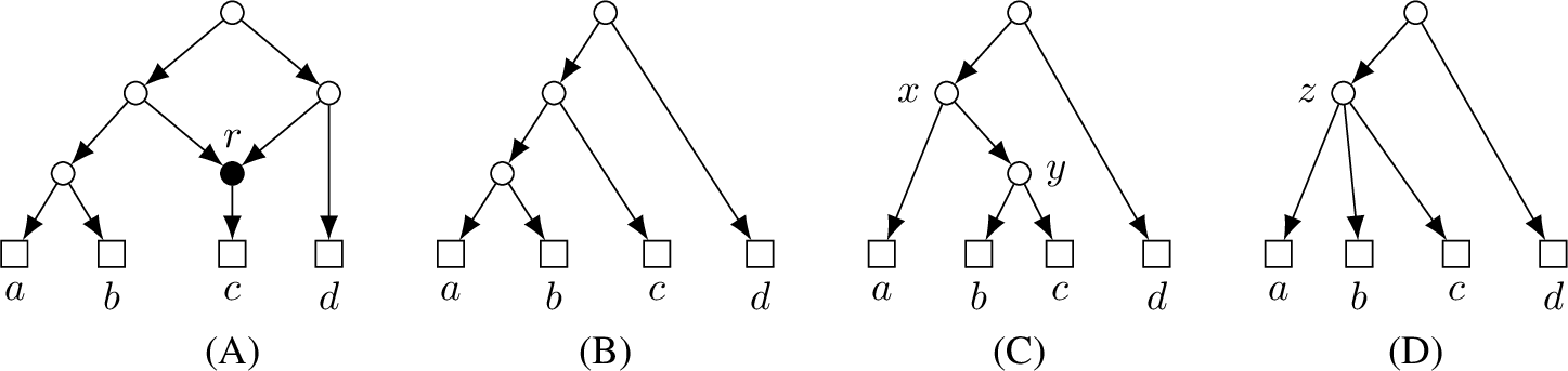
To address this limitation, a relaxed version of Tree Containment, called Soft Tree Containment, was proposed by Bentert and Weller [16]. This relaxed framework allows “undoing” contractions of poorly supported branches (contracting low-support branches is a common preprocessing step in network analysis), effectively allowing uncertainty in the form of so-called “soft polytomies”. The corresponding notion of “soft display” (see 5) permits us to resolve each high-degree vertex into a binary tree. Then, the resulting binary resolution of the network ought to firmly display the resulting binary resolution of the tree.

Although Soft Tree Containment, like Tree Containment, remains NP-hard [16], we aim to solve even large instances in practice. To achieve this, we leverage the fact that phylogenetic networks occurring in empirical studies are expected to exhibit a certain degree of tree-likeness, which can be effectively quantified using the recently introduced measure of tree-likeness called “scanwidth” [17]. Our algorithm solves Soft Tree Containment in \(2^{\mathcal{O}(\Delta_{T} \cdot k \cdot \log(k))} \cdot n^{\mathcal{O}(1)}\) time, where \(k \mathrel{\vcenter{:}}=\mathop{\mathrm{sw}}(\Gamma) + \Delta_{N}\), with \(\Delta_{T}\) and \(\Delta_{N}\) denoting the maximum out-degrees in the tree and the network, respectively, and \(\mathop{\mathrm{sw}}(\Gamma)\) denoting the scanwidth of a tree extension that is given as part of the input. (Tree extensions resemble tree decompositions and will be defined formally later.) The algorithm first makes the network binary through “stretching” and “in-splitting”. This special case (where the network is binary but the tree need not be) is then solved via bottom-up dynamic programming along the given tree extension.

2 Related Work↩︎

On a binary network \(N\) and a binary tree \(T\), the Tree Containment problem can be solved in \(2^{\mathcal{O}(t^2)} \cdot \lvert A(N)\rvert\) time, where \(t\) denotes the treewidth of \(N\) and \(A(N)\) is its arc set [18]. This special case of Tree Containment is also a special case of Soft Tree Containment, as the notions of “firm” and “soft” display coincide when \(N\) and \(T\) are both binary [19]. Additionally, Soft Tree Containment is a generalization of the Cluster Containment problem [19]. Van Iersel, Semple, and Steel [8] show that the latter problem can be solved in polynomial time on binary networks of constant “level”. Note that level-\(c\) networks have scanwidth at most \(c + 1\) [20]. A comparison of the level, scanwidth, and treewidth of real-world phylogenetic networks was conducted by Holtgrefe [20], concluding that treewidth is not much smaller than scanwidth in practice. He further points out that “edge-treewidth” by Magne et al. [21] is the undirected analogue of scanwidth. We also remark that Soft Tree Containment is conceptually similar to Minor Containment: The question of whether a binary network \(N\) softly displays a possibly non-binary tree \(T\) is equivalent to asking if \(T\) can be obtained from a subtree of \(N\) through arc contraction (while preserving leaf-labels). In fact, the reduction of general Soft Tree Containment to this special case is the subject of 4.2. Janssen and Murakami [22] study a similar containment notion based on arc contraction.

3 Preliminaries↩︎

3.0.0.1 Directed Graphs.

A directed graph (or digraph for short) is an ordered pair \(D = (V, A)\) that consists of a non-empty, finite set \(V\) of vertices and a set \(A \subseteq \{(u, v) \in V^2 \mid u \neq v\}\) of arcs. We also use the notation \(V(D) \mathrel{\vcenter{:}}= V\) and \(A(D) \mathrel{\vcenter{:}}= A\). The in-neighbors of a vertex \(v \in V\) are referred to as its parents (denoted \(V^-_D (v)\)), and its out-neighbors are referred to as its children (denoted \(V^+_D (v)\)). The set of incoming arcs of \(v\) is denoted \(A^-_D (v)\), and the set of outgoing arcs of \(v\) is denoted \(A^+_D (v)\). The in-degree of \(v\) is \(\deg^-_D (v) \mathrel{\vcenter{:}}=\lvert V^-_D (v)\rvert\), the out-degree of \(v\) is \(\deg^+_D (v) \mathrel{\vcenter{:}}=\lvert V^+_D (v)\rvert\), and the degree of \(v\) is \(\deg_D (v) \mathrel{\vcenter{:}}=\deg^-_D (v) + \deg^+_D (v)\). The maximum out-degree of any vertex in \(D\) is denoted \(\Delta_{D}\). If the maximum in-degree and the maximum out-degree of \(D\) are both at most \(2\), then \(D\) is called binary. Note that this definition permits a vertex in a binary digraph to have in-degree \(1\) and out-degree \(1\) simultaneously, and also in-degree \(2\) and out-degree \(2\) simultaneously, making it slightly more permissive than the definition often used in phylogenetics that requires every non-root non-leaf vertex in a binary digraph to have degree exactly \(3\). We define the terms root and leaf in a digraph as follows: A root of \(D\) is a vertex with in-degree \(0\), and \(D\) is called rooted if it has exactly one root (denoted \(\mathop{\mathrm{root}}(D)\)). A leaf of \(D\) is a vertex with out-degree \(0\), and the set of all leaves of \(D\) is denoted \(L(D)\). We use \({\geq_D} \subseteq V^2\) to denote the reachability relation of \(D\) (so \(u \geq_D v\) means that there is a directed path from \(u\) to \(v\), possibly having length \(0\)). The irreflexive kernel of \(\geq_D\) is denoted \(>_D\). We say that \(D\) is weakly connected if the underlying graph of \(D\) is connected. The result of removing \(v\) from \(D\) is denoted \(D - v\). We also use the notation \(D - U\) when removing a set of vertices \(U\) from \(D\). If a digraph \(D'\) can be obtained by removing vertices and arcs from \(D\), then \(D'\) is a subdigraph of \(D\), denoted \(D' \subseteq D\), and \(D'\) is called leaf-monotone if, additionally, \(L(D')\subseteq L(D)\). The subdigraph induced by a non-empty set \(U \subseteq V\) is \(D[U] \mathrel{\vcenter{:}}=(U, \{(u, v) \in A \mid u, v \in U\})\). When subdividing an arc \((u, v) \in A\) with a new vertex \(w \notin V\), the arc \((u, v)\) is removed from \(D\), while the vertex \(w\) and the arcs \((u, w)\) and \((w, v)\) are added. The inverse operation, removing \(w\) with its incident arcs and adding \((u, v)\), is called suppression of \(w\). When contracting \((u, v)\), the parents of \(v\), except for \(u\), become parents of \(u\), and the children of \(v\), except for possibly \(u\), become children of \(u\); the vertex \(v\) and its incident arcs are then removed. If \(D\) can be obtained from a digraph \(D'\) by subdividing arcs, then \(D\) is a subdivision of \(D'\). The union of two digraphs \(D\) and \(D'\) is \(D \cup D' \mathrel{\vcenter{:}}=(V(D) \cup V(D'), A(D) \cup A(D'))\). A directed acyclic graph (DAG) is a digraph without directed cycles. An out-tree is a rooted DAG in which every vertex has in-degree at most \(1\).

3.0.0.2 Phylogenetic Networks.

A (phylogenetic) network is a rooted DAG whose root has out-degree at least \(2\) and in which each non-root vertex either has in-degree \(1\) (and is called a tree vertex) or has out-degree \(1\) (and is called a reticulation), but not both (see 1 (A)). The root of a network is also considered to be a tree vertex. If a network has no reticulations (that is, it is an out-tree), then it is called a (phylogenetic) tree.

3.0.0.3 Scanwidth.

Undoubtedly, one of the most successful concepts in algorithmic graph theory is the notion of treewidth [23]. While some problems in phylogenetics yield efficient algorithms on networks of bounded treewidth, the “undirected nature” of treewidth often makes dynamic programming prohibitively complicated or outright unimplementable [24]. Since phylogenetic networks exhibit a “natural flow of information” along the direction of the arcs, Berry, Scornavacca, and Weller [17] introduced a width measure similar to treewidth, but respecting the direction of the arcs (see [25], [26] for previous efforts to port the notion of treewidth to directed graphs), called “scanwidth”. The idea is to “inscribe” the arcs of the network \(N\) into an out-tree \(\Gamma\) (called a “tree extension”) on \(V(N)\), such that all network arcs are directed away from the root of \(\Gamma\) (see 2). This structure allows a bottom-up dynamic-programming approach whose exponential part depends on the size of the set \(\mathop{\mathrm{GW}}_v (\Gamma)\) of arcs of \(N\) that would be cut when slicing just above any vertex \(v\) of \(\Gamma\).

We now give a more comprehensive account of scanwidth and define it formally. Let \(D\) be a DAG. The purpose of scanwidth is to measure how similar \(D\) is to an out-tree. This is motivated by the observation that algorithmic problems can often be solved efficiently on (out-)trees, with the hope that this generalizes to DAGs that have low scanwidth (and are, thus, “similar” to out-trees). Specifically, low scanwidth is supposed to ensure that bottom-up dynamic programming works like on out-trees: Solutions for separate subtrees can be computed independently, and these solutions can be combined efficiently once the parent that connects the subtrees is encountered. Since \(D\) is an arbitrary DAG and not necessarily an out-tree, we first need an appropriate notion of “subtree”. For scanwidth, the subtrees to consider are those of a tree extension of \(D\), which is an out-tree \(\Gamma\) on \(V(\Gamma) = V(D)\) with \(A(D) \subseteq {>_\Gamma}\). That is, the out-tree \(\Gamma\) has the same vertex set as \(D\) and, for every arc \((u, v)\) of \(D\), there is a directed path from \(u\) to \(v\) in \(\Gamma\). This ensures that reachability in \(D\) implies reachability in \(\Gamma\) (but there is generally no direct correspondence between arcs of \(D\) and arcs of \(\Gamma\)). Note that tree extensions generalize topological orderings, and so every DAG has at least one tree extension (which may be a directed path corresponding to a topological ordering).

So we want to solve algorithmic problems on \(D\) via bottom-up dynamic programming along \(\Gamma\), where separate subtrees of \(\Gamma\) represent parts of \(D\) that should be solved independently. Crucially, we need to be able to extend solutions for small subtrees to obtain solutions for larger subtrees. For this to work efficiently, we want the vertices of each subtree of \(\Gamma\) to represent a part of \(D\) that is mostly “self-contained” in the sense that only few arcs in \(D\) cross into the part from the outside. For the subtree of \(\Gamma\) rooted at a vertex \(t \in V(\Gamma)\), these are precisely the arcs of the set \(\mathop{\mathrm{GW}}^D_t (\Gamma) \mathrel{\vcenter{:}}=\{(u, v) \in A(D) \mid u >_\Gamma t \geq_\Gamma v\}\).² We want even the largest of these sets to be small, and so we define \(\mathop{\mathrm{sw}}_D (\Gamma) \mathrel{\vcenter{:}}=\max_{t \in V(\Gamma)} \lvert\mathop{\mathrm{GW}}^D_t (\Gamma)\rvert\). Then, the scanwidth of \(D\), denoted \(\mathop{\mathrm{sw}}(D)\), is the minimum \(\mathop{\mathrm{sw}}_D (\Gamma)\) over all tree extensions \(\Gamma\) of \(D\).

Scanwidth can be visualized via “scanner lines”, explaining its name: First, lay out the vertices of \(D\) according to \(\Gamma\), where the root of \(\Gamma\) is at the top and the leaves of \(\Gamma\) are at the bottom. Second, draw the arcs of \(D\). The definition of a tree extension ensures that all arcs of \(D\) now point downward. Third, imagine horizontal scanner lines, one above each leaf of \(\Gamma\). Every scanner line cuts through some set of arcs of \(D\). We observe which arcs are cut as a scanner line moves through the drawing from bottom to top, where distinct scanner lines merge into one scanner line once they meet at a vertex. Indeed, the arcs cut by a scanner line that is directly above a vertex \(t \in V(\Gamma)\) are precisely those of the set \(\mathop{\mathrm{GW}}^D_t (\Gamma)\). We will also be interested in the arcs that are cut by scanner lines directly below the vertex \(t\). These are given by the set \(\mathop{\mathrm{HW}}^D_t (\Gamma) \mathrel{\vcenter{:}}=\{(u, v) \in A(D) \mid u \geq_\Gamma t >_\Gamma v\}\). The scanner-line visualization is depicted in 2.

For the purpose of dynamic programming, it will be helpful to assume that we are given a tree extension with special structure: If \(D\) is rooted, then a canonical tree extension \(\Gamma\) of \(D\) is such that \(D[\{v \in V(D) \mid t \geq_\Gamma v\}]\) is weakly connected for all \(t \in V(\Gamma)\) [20]; that is, the part of \(D\) represented by the vertices of the subtree of \(\Gamma\) that is rooted at \(t\) is always weakly connected. This is desirable because it guarantees that \(L(\Gamma) = L(D)\) and \(\deg^+_\Gamma (v) \leq \deg^+_D (v)\) for each \(v \in V(D)\) [17]. In particular, if \(D\) is binary, then so is \(\Gamma\). These properties hold in a canonical tree extension because a vertex \(v\) with greater out-degree in \(\Gamma\) than in \(D\) would be the root of a subtree of \(\Gamma\) corresponding to a part of \(D\) that is not weakly connected. The assumption that a given tree extension is canonical comes at no cost with respect to scanwidth, and only minor cost in running time: Given a non-canonical tree extension \(\Gamma\) of a rooted DAG \(D\), a canonical tree extension \(\Gamma'\) of \(D\) with \(\mathop{\mathrm{sw}}_D (\Gamma') \leq \mathop{\mathrm{sw}}_D (\Gamma)\) can be constructed in polynomial time [20].

Assuming that no ambiguity arises, we may omit sub- or superscripts.

4 Deciding Soft Tree Containment↩︎

In this paper, we develop a parameterized algorithm for Soft Tree Containment. Informally speaking, this problem, first considered by Bentert, Malík, and Weller [19], asks us to decide if a given phylogenetic tree can be embedded in a given phylogenetic network while taking into account uncertainty in the form of soft polytomies (high-degree vertices to be resolved into a binary tree). We build up to its formal definition ([prob:stc]) in a way that differs slightly from the original. First, we adapt the notion of splitting [16], [22].

Exhaustive out-splitting enables us to resolve a high-out-degree tree vertex into a binary out-tree. Its dual for high-in-degree reticulations is defined below. The definitions are illustrated in 3.

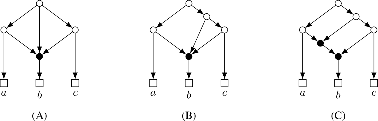
We now introduce terminology for partially and fully resolved networks. Note that we use a different definition of binary resolution than Bentert, Malík, and Weller [19]. This avoids corner cases violating the intuition behind soft polytomies.

Note that, to obtain a binary resolution, it does not matter whether in-splitting is performed before out-splitting or after; the order is arbitrary.

When discussing firm and soft display, we want to treat leaves as labeled and all other vertices as unlabeled. This is achieved via the following notion of an isomorphism that agrees with the identity function on all leaves.

At this point, we have everything needed to define the central notions of display for this work. Recall that, when taking a leaf-monotone subdigraph, no new leaves can be created.

We are now ready to define the problem under consideration. Note that, for technical reasons, we restrict the input slightly more than Bentert, Malík, and Weller [19]; in particular, networks in our sense cannot contain any vertex that has both in-degree and out-degree \(1\). We believe the problem to become computationally harder with such vertices permitted, despite their insignificance in practice.

A phylogenetic network \(N\) and a phylogenetic tree \(T\) with \(L(T) \subseteq L(N)\). Does \(N\) softly display \(T\)? [19]

We solve this problem in two steps, corresponding to the next two sections. In 4.1, we consider the special case where the given network \(N\) is binary. In 4.2, we describe a reduction mapping an arbitrary network to a binary one.

A \(\mathtt{YES}\)-instance and a \(\mathtt{NO}\)-instance of Soft Tree Containment are depicted in 4. The figure also illustrates some of the notions defined and used in 4.1.

4.1 Soft Display by Binary Networks↩︎

Van Iersel, Jones, and Weller [15] present a dynamic-programming algorithm that uses tree extensions, thereby leveraging low scanwidth, to solve the Tree Containment problem, which asks for firm rather than soft containment. In the following, we adapt their algorithm for our purposes. Although our approach closely follows theirs, the presentation we give here is self-contained. We will highlight both similarities and differences between the two approaches. To start with, we use their definition of a downward-closed subforest and of top arcs in \(T\), which are mapped into the “bags” of a given tree extension of \(N\).

In contrast to the definition of a phylogenetic network/tree, it will be more convenient to work with \(N\) and \(T\) whose roots have out-degree \(1\). This is for technical reasons, a standard practice, and does not limit practical applicability. We also assume to be given a tree extension, ideally of low scanwidth, which might be more problematic in practice, but it allows us to separate the problem of computing/approximating low-scanwidth tree extensions from the problem of deciding soft containment. The following assumption formally introduces these objects, but its scope is restricted to this section and we drop it for 4.2.

We generalize the strict reachability relation defined earlier in order to define reachability between arcs and vertices/arcs. The new reachability relation agrees with the old relation when comparing two vertices.

This relation lets us describe parts of \(N\) or \(T\) that are “below” a specified set of arcs. In particular, our dynamic-programming table will indicate whether the parts of \(T\) that are below an anti-chain of arcs (called “top arcs”) can be embedded below a set of arcs in \(N\) (see 4).

In contrast to firm containment, soft containment allows embedding distinct arcs \((x, y)\) and \((x, z)\) of \(T\) as paths in \(N\) that may start with the same arcs but separate further down. We call such paths eventually arc-disjoint.

We remark that the union of several pairwise eventually arc-disjoint paths that all start with the same vertex can be used to form an out-tree. To witness soft containment, we associate each vertex of \(T\) with such a collection of paths in \(N\). Formalizing this intuition, we adapt the notion of a pseudo-embedding [15] to work with eventually arc-disjoint paths. Then, we show that such an embedding of \(T\) into \(N\) witnesses \(N^*\) softly displaying \(T^*\).

If there is a pseudo-embedding (in the sense of Van Iersel, Jones, and Weller [15]) of a downward-closed subforest of \(T\) into \(N\), then it is a soft pseudo-embedding as well, but not vice versa. We have to use this more general notion because Soft Tree Containment is intentionally more permissive than Tree Containment. In fact, handling these generalized embeddings is the primary novelty of the dynamic-programming algorithm that we develop in this section (6): We inherit the idea of computing embeddings of parts of \(T\) that are below a top-arc set into parts of \(N\), where we only store how each top arc is to be embedded in a “bag” of \(\Gamma\), but the details differ significantly for Soft Tree Containment. Crucially, a soft pseudo-embedding can map two distinct arcs to paths that share some arcs; the paths might only be eventually arc-disjoint. This changes how we generate the embeddings and, thus, changes the analysis. Moreover, our generalized embeddings can be more numerous (compare [lem:vsigbound] with [15]). We prove now that these generalized embeddings indeed capture Soft Tree Containment.

Recall that we assume to be given a canonical tree extension \(\Gamma\) of \(N\) (see 1) and that we define \(\mathop{\mathrm{HW}}_t (\Gamma) \mathrel{\vcenter{:}}=\{(u, v) \in A(N) \mid u \geq_\Gamma t >_\Gamma v\}\) for every \(t \in V(\Gamma)\). When visualizing scanwidth via scanner lines (see 2), the set \(\mathop{\mathrm{HW}}_t (\Gamma)\) may be thought of as containing the arcs of \(N\) cut directly below \(t \in V(\Gamma)\), whereas \(\mathop{\mathrm{GW}}_t (\Gamma)\) contains the arcs cut directly above \(t\).

In the following, we develop a dynamic-programming algorithm that computes its table entries (“signatures”) bottom-up along \(\Gamma\). Intuitively, for each vertex \(t \in V(\Gamma)\), each top-arc set \(S\) in \(T\), and each \(\psi \colon S \to \mathop{\mathrm{GW}}_t (\Gamma)\), we set the table entry / signature \([\mathop{\mathrm{GW}}_t (\Gamma), S, \psi]\) to “valid” if the forest below \(S\) in \(T\) is softly displayed by the network below \(\mathop{\mathrm{GW}}_t (\Gamma)\) in such a way that each arc \(a \in S\) is embedded in a path starting with \(\psi(a) \in \mathop{\mathrm{GW}}_t (\Gamma)\). An example of a valid signature is depicted in 5. Note that \(\psi\) is not required to be injective.

Our dynamic-programming algorithm, 6, decides whether \(N^*\) softly displays \(T^*\) by, in some sense, exhaustively generating valid signatures. Once it has generated them, it can easily read off the final answer ([lem:vsigtoparc]). To prove the main result of this section (1), we establish the correctness of 6 and bound its running time. This involves showing that 6 generates its valid signatures correctly ([lem:vsigleaf] [lem:vsigHW] [lem:vsigGW]) and that there are not too many valid signatures to generate ([lem:vsigbound]). We start with the latter.

For every non-root vertex \(v \in V(\Gamma)\), 6 constructs the set \(\mathit{GWS}_v\) of pairs \((S, \psi)\) for which \([\mathop{\mathrm{GW}}_v (\Gamma), S, \psi]\) is a valid signature (and analogously for \(\mathit{HWS}_v\)). The construction has three steps: First, handling the case where \(v\) is a leaf. Second, constructing \(\mathit{HWS}_v\) when \(v\) is not a leaf. Third, constructing \(\mathit{GWS}_v\) when \(v\) is not a leaf. The next three lemmas imply the steps’ correctness.

Recall that \(N\) is binary. Since \(\Gamma\) is canonical, it too is binary in consequence [17], and so any vertex has at most two children in \(\Gamma\). For every non-root, non-leaf \(v \in V(\Gamma)\), 6 constructs \(\mathit{HWS}_v\) by combining pairs from \(\mathit{GWS}_{q_1}\) and \(\mathit{GWS}_{q_2}\), where \(q_1\) and \(q_2\) are the children of \(v\) in \(\Gamma\). We define \(D_u \mathrel{\vcenter{:}}= D[\{w \in V(D) \mid u \geq_D w\}]\) for each \(u \in V(D)\) in a DAG \(D\), to refer to subtrees of \(T\) and \(\Gamma\). Recall that \(\psi |_Z\) is the restriction of \(\psi\) to \(Z\).

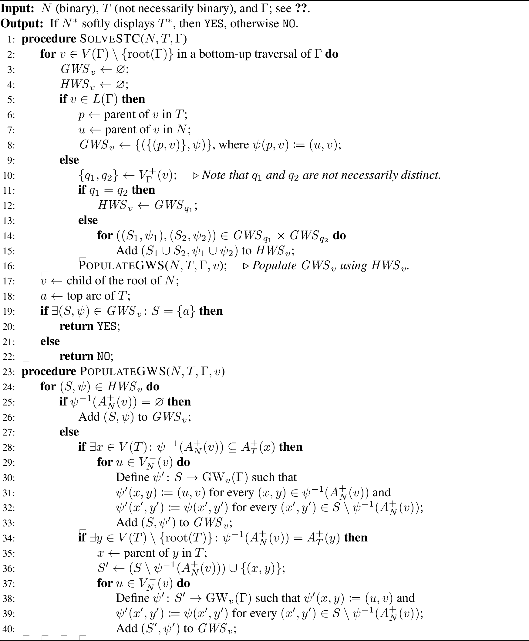
The next lemma concerns the correctness of the procedure PopulateGWS. Given a non-root, non-leaf vertex \(v \in V(\Gamma)\), this procedure constructs the set \(\mathit{GWS}_v\) based on the elements of \(\mathit{HWS}_v\). Informally speaking, this step from \(\mathop{\mathrm{HW}}_v (\Gamma)\) to \(\mathop{\mathrm{GW}}_v (\Gamma)\) unlocks the incoming arcs of \(v\) in \(N\). There are three ways in which these arcs may be used: (1) not at all, (2) to elongate paths of an existing embedding, or (3) to enlarge the downward-closed subforest to be embedded.

1.  $X \mathrel{\vcenter{:}}=\psi^{-1} (u, v) \subseteq A^+_T (x)$
    for some $x \in V(T)$, and

2.  $[\mathop{\mathrm{HW}}_v (\Gamma), S, \psi']$ is a valid
    signature, where
    $\psi' \colon S \to \mathop{\mathrm{HW}}_v (\Gamma)$ is some
    function with $\psi'(X) \subseteq A^+_N (v)$ and, for all
    $(x', y') \in S \setminus X$, we have
    $\psi'(x', y') = \psi(x', y')$.

1.  $y \notin L(T)$, and

2.  $[\mathop{\mathrm{HW}}_v (\Gamma), S_{x, y}, \psi']$ is a valid
    signature, where
    $S_{x, y} \mathrel{\vcenter{:}}=(S \setminus \{(x, y)\}) \cup A^+_T (y)$
    and $\psi' \colon S_{x, y} \to \mathop{\mathrm{HW}}_v (\Gamma)$
    is some function with $\psi'(A^+_T (y)) \subseteq A^+_N (v)$
    and, for all $(x', y') \in S \setminus \{(x, y)\}$, we have
    $\psi'(x', y') = \psi(x', y')$.

While the previous lemmas established that 6 constructs its valid signatures correctly (that is, the \((S, \psi)\) pairs it generates correspond precisely to the valid signatures of interest), the next lemma implies that its final answer is correct.

We now piece the previous lemmas together to conclude this section.

Note that 6 decides Soft Tree Containment without explicitly constructing a full soft pseudo-embedding of \(T\) into \(N\). However, it is not difficult to adapt the algorithm so as to output such a soft pseudo-embedding on a \(\mathtt{YES}\)-instance: Let \(v \in (V(\Gamma) \setminus \{\mathop{\mathrm{root}}(\Gamma)\}) \setminus L(\Gamma)\). Simply have the algorithm store, for each pair \((S, \psi) \in \mathit{GWS}_v\), a single pair from \(\mathit{HWS}_v\) from which \((S, \psi)\) was constructed. Similarly, have the algorithm store, for each pair in \(\mathit{HWS}_v\), the one or two pairs from which it was constructed. In case of a \(\mathtt{YES}\)-instance, these separately stored pairs would allow the algorithm, at the end, to construct a soft pseudo-embedding of \(T\) into \(N\) through backtracing.

4.2 Soft Display by Arbitrary Networks↩︎

In this section, we devise a reduction that maps any network to a binary one while preserving the trees that the network softly displays. The reduction can be performed in polynomial time, and the resulting increase in the scanwidth of the network can be bounded. Relying on the considerations of the previous section, we then obtain our main result (1). The reduction consists of two steps:

1. We stretch the network. This means that we modify the network using gadgets that are conceptually very similar to the universal networks by Zhang [28] (see 7, also compare [28]). Like these universal networks, our gadgets consist of a triangular upper part and a lower part that is based on a sorting network.

   The triangular upper part is essentially one half of a grid that was slightly modified to obtain a phylogenetic network. In it, any binary phylogenetic tree (up to some number of leaves) can be embedded. As each high-out-degree vertex is replaced by a gadget when stretching, the stretched network represents all possible binary out-resolutions.

   However, embedding a binary tree in the triangular upper part artificially enforces an order on the leaves of the binary tree. The lower part allows us to undo this. We choose a different sorting network than Zhang [28].

2. We compute an arbitrary binary in-resolution of the stretched network through exhaustive in-splitting. This does not affect which trees are firmly displayed.

The purpose of stretching, defined below, is to get rid of vertices with high out-degree in a network, so that we can assume the resulting network to have maximum out-degree \(2\).

In the appendix, we provide an equivalent definition where the vertices and the arcs of a stretch gadget are listed explicitly (12).

An anonymous reviewer suggested a simple alternative to stretching that, in a network \(N\), below any vertex \(v\) of out-degree \(d \geq 1\) with children \(c_1, c_2, \dots, c_d\), inserts a recursively defined gadget \(G_d\) instead (again replacing the outgoing arcs of \(v\)): If \(d = 1\), then \(G_d\) simply consists of \(v\) and its child \(c_1\), with the arc in between exactly as it exists in \(N\). If \(d \geq 2\), then \(G_d\) is constructed by first inserting the gadget \(G_{d - 1}\) between \(v\) and children \(c_1, c_2, \dots, c_{d - 1}\), and then subdividing each arc \(a\) of \(G_{d - 1}\) with a new vertex \(u_a\). Finally, arcs from every \(u_a\) to \(c_d\) are added. Note that, in the end, \(v\) has a single outgoing arc. To obtain a phylogenetic network, this arc needs to be contracted if \(d \geq 2\), but only once, after the recursion is fully done. This gadget mimics the property that removing a leaf from a tree with \(k \geq 3\) leaves produces what is essentially a subdivision of a tree with \(k - 1\) leaves (but its root may now have out-degree \(1\)).

These alternative gadgets can be described simply and concisely; however, they can cause an increase in scanwidth that is exponential in the initial maximum out-degree of the network. This is because, to add one more child, the number of arcs of the gadget is doubled through subdivision. The next child to add then has high in-degree, which causes the gadget to have high scanwidth. To obtain the running time reported in 1, we use stretch gadgets, since these can only cause an increase in scanwidth that is linear in the initial maximum out-degree of the network ([lem:swstr]).

The proof of 1 relies on four key claims: [lem:strsd] [lem:binressd], which state that stretching and in-splitting preserve the collection of trees softly displayed a network, and [lem:swstr] [lem:swin], which state that the increase in scanwidth when stretching and in-splitting is bounded, using the network’s maximum out-degree. To prove [lem:strsd], we first formalize the intuition that the stretched network “represents” all possible binary out-resolutions.

With 1 at hand, we now show that stretching preserves the collection of trees that a network softly displays.

We argue that a stretched network can be made binary through in-splitting without altering the collection of softly displayed trees; the collection of firmly displayed trees also stays unaltered. In stretched networks, the maximum out-degree is \(2\); that is, we can assume that \(\Delta_{N} = 2\). The in-degrees, however, are generally unbounded. The lemma below justifies arbitrary in-splitting (taking any binary (in-)resolution) to make a stretched \(N\) binary indeed.

Finally, we show that neither stretching nor in-splitting to obtain a binary in-resolution can blow up the scanwidth too much, in order to prove 1.

The last ingredient for 1 is the monotonicity of scanwidth under in-splitting.

We finish with the main result of this paper.

5 Conclusion↩︎

We devised a parameterized algorithm for the Soft Tree Containment problem, where it has to be decided whether a phylogenetic network softly displays a phylogenetic tree. This algorithm consists of two steps: solving the problem via dynamic programming when the network is binary and reducing any non-binary network to an equivalent binary one. The running time of this algorithm depends exponentially on a function of the network’s and the tree’s maximum out-degree and of the scanwidth attained by a given tree extension of the network. The dependence on the input size is polynomial.

Future work can attempt to eliminate the superpolynomial dependence on the maximum out-degrees or, alternatively, rule out the existence of such an algorithm. Because of the dependence on scanwidth, it is essential to be able to obtain low-scanwidth tree extensions in a reasonable amount of time. This further motivates the search for exact or approximate algorithms to construct such tree extensions. Additionally, it is of interest to tackle Soft Tree Containment with parameters stronger than scanwidth, such as node-scanwidth [20], edge-treewidth [21], or treewidth. Even weaker parameters could be of interest, when they give rise to algorithms that perform better in practice for example. Finally, it is worth exploring whether our techniques can be adapted to approach other containment problems, for instance, Network Containment in the sense of Janssen and Murakami [22].

6 Stretching↩︎

In the following, we list the vertices and arcs of a stretch gadget explicitly (compare with 11). We hope that this can aid in possible implementation projects.

References↩︎