1 Introduction↩︎

Nakajima [4] invented Nakajima quiver varieties and initiated the study of the relation between the moduli space of instantons and vertex operator algebras (VOA for short). Vafa–Witten [1] tested S-duality (Montonen–Olive duality) via mathematical works like [2]–[8], and found unexpected links between supersymmetric Yang-Mills theory and 2-dimensional conformal field theory (2d CFT for short). In this paper, we confirm a major prediction made by [1] that relates Yoshioka’s blow-up formula to the WZW models of \(\mathrm{SU}(r)\) at level \(1\).

1.1 S-duality and modularity↩︎

To explain the main results of the paper, we first recall the S-duality conjecture from a mathematical perspective, following [9]. The idea of S-duality can be traced back to Maxwell’s equations, which exhibit symmetry under swapping electric and magnetic fields. In the non-abelian case, it was generalized by Montonen–Olive [10] in the \(N=4\) supersymmetric gauge theory and is called Montonen–Olive duality, or the S-duality conjecture. In [1], Vafa–Witten studied the partition functions of the 4-dimensional \(N=4\) supersymmetric theory for a compact 4-dimensional manifold \(S\) with gauge group \(\mathrm{G}\). When \(\mathrm{G}=\mathrm{SU}(r)\) and \(S\) is a smooth projective surface with some vanishing conditions, such as \[\begin{align} \label{assumptionS} & K_S\cong \mathcal{O}_S \text{ or } K_S\cdot H<0 \end{align}\tag{1}\] which are always satisfied when \(S\) is a \(K3\) surface, an abelian surface, or a del Pezzo surface, the partition function is the generating function of the Euler characteristics of the moduli space of \(H\)-stable coherent sheaves on \(S\) with rank \(r\) and fixed first Chern class¹. Let \(\mathrm{Z}(S,\mathrm{G},\tau)\) be the partition function, with \(q=e^{2\pi i \tau}\), where \(q\) is the formal variable in the generating function. The S-duality conjecture asserts that \[\mathrm{Z}(S,\mathrm{G}, \tau)=\pm r^{\chi(S)/2}(\frac{\tau}{i})^{w/2}\mathrm{Z}(S, ^L\mathrm{G}, -1/\tau),\] where \(w\) is a constant that depends only on \(S\), \(\chi(S)\) is the topological Euler number of \(S\), and \(^L\mathrm{G}\) is the Langlands dual group of \(\mathrm{G}\). When \(\mathrm{G}=\mathrm{SU}(r)\), we have \(^L\mathrm{G}=\mathrm{SU}(r)/\mu_r\), where \(\mu_r\) is the group of the \(r\)-th root of unity. Then S-duality conjecture reveals the modularity of the partition function, which suggests an unexpected relation to 2d CFT.

In particular, Vafa–Witten made several tests based on the mathematical work [2]–[8]. When \(S\) is a K3 surface, the formal series generated by the Euler characteristic is the partition function of the bosonic string by Mukai [5] and Göttsche [13], and Vafa–Witten suggested a relation with the Fock space. When \(S=\mathbb{CP}^2\), the partition function is modular only after a natural non-holomorphic modification due to Yoshioka [2], [3], and Vafa–Witten suggested that such a modification should be related to a holomorphic anomaly in certain two-dimensional models. When \(S\) is an ALE space, Nakajima [4] constructed the action of the Kac-Moody algebra on the equivariant cohomology groups of the moduli space of framed sheaves on \(S\), through the novel construction of the Hecke correspondences on the Nakajima quiver varieties. Vafa–Witten raised the question to explain Nakajima’s work in the framework of S-duality, as ALE spaces are not compact.

In the past decades, there have been substantial advances on the above questions, except the following question which relates the blow-up formula of Yoshioka with the WZW model of \(\mathrm{SU}(r)\) at level \(1\): when \(S\) is a smooth projective surface, let \(\hat{S}\) be the blow-up of \(S\) along a closed point \(o\). Given a total Chern class \(c\), let \(\mathcal{M}_H(c)\) and \(\mathcal{M}_{H_{\infty}}(\hat{c})\) be the moduli spaces of Gieseker-stable sheaves on \(S\) and \(\hat{S}\), respectively (the detailed definition will be given in 1.2). In [2], [3], Yoshioka proved a blow-up formula for the Betti numbers of \(\mathcal{M}_{H}(c)\) and \(\mathcal{M}_{H_{\infty}}(\hat{c})\) when the rank is \(2\), and if we only consider the Euler characteristics, the formula can be written as \[\label{eq:Yoshioka} \frac{\sum_{n}\chi(\mathcal{M}_{H_\infty}(2,p^*c_1-a[C],n))q^{n+a/4}}{\sum_{n}\chi(\mathcal{M}_{H}(2,c_1,n))q^{n}}=\frac{\theta_a(q)}{\eta(q)^2}, \quad a=0,1,\tag{2}\] where \(p:\hat{S}\to S\) is the projection map, \([C]\) is the exceptional divisor, and \[\theta_a(q):=\sum_{n\in \mathbb{Z}+a/2}q^{n^2}, \text{ and } \eta(q):=q^{1/24}\prod_{n\geq 1}(1-q^n)\] are the Jacobi theta function and the Dedekind eta function, respectively. Vafa–Witten [1] observed that the formula is related to the character of the WZW model of \(\mathrm{SU}(2)\) at level \(1\), and highlighted the unresolved mystery of the appearance of a 2d CFT in this context and its generalization to higher-rank cases.

In this paper, we give a full answer to this question by constructing the affine \(\mathrm{gl}_r\)-action on various cohomology theories of \(\mathcal{M}_{H_\infty}(\hat{c})\) and identifying the module as a basic representation. The detailed statement of the main results will be given in 1.2.

1.2 The main results of the paper↩︎

Given an ample line bundle \(H\) and a total Chern class \(c=(r,c_1,n)\), let \(\mathcal{M}_H(c)\) be the moduli space of Gieseker-stable sheaves on \(S\) with total Chern class \(c\). For any \(1\gg \epsilon>0\), the \(\mathbb{Q}\)-divisor \(p^*H-\epsilon C\) is also ample, and the moduli space \(\mathcal{M}_{p^*H-\epsilon C}(\hat{c})\) stabilizes as \(\epsilon\to 0\) for any given total Chern class \(\hat{c}\) on \(\hat{S}\); we denote it by \(\mathcal{M}_{H_\infty}(\hat{c})\). Yoshioka’s blow-up formula 2 was generalized by the second-named author and Qin [14], [15] to virtual Hodge numbers, where the moduli space may be singular, and by Nakajima–Yoshioka [16], [17] to arbitrary ranks. For example, for the rank \(2\) case we have \[\frac{\sum_{n}h^{i,j}(\mathcal{M}_{H_\infty}(2,p^*c_1-a[C],n))x^iy^jq^{n+a/4}}{\sum_{n}h^{i,j}(\mathcal{M}_{H}(2,c_1,n))x^iy^jq^{n}} = q^{1/12}Z_a(x,y,q),\] where \(a=0,1\), \(h^{i,j}\) is the (virtual) Hodge number and \[\label{theta-fun} Z_a(x,y,q)=\frac{\sum_{n\in \mathbb{Z}}(xy)^{\frac{(2n+a)^2-(2n+a)}{2}}q^{(2n+a)^2/4}}{q^{1/12}\prod_{n\geq 1}(1-(xy)^{2n}q^n)^2},\tag{3}\] so that \(Z_a(x,1/x,q)=\frac{\theta_a(q)}{\eta(q)^2}\). Nakajima–Yoshioka [18] studied the equivariant cohomology of the moduli space of framed sheaves over \(\mathbb{P}^2\), and constructed a basic representation of the affine Lie algebra \(\hat{\mathrm{gl}}_r\) on the blow-up through localization. It provided a rational CFT construction for \(S=\mathbb{P}^2\), as there is a correspondence between the WZW model and the basic representation through the affine vertex algebra (we refer to [19] for details of this correspondence). For the general case, including unframed moduli spaces of stable coherent sheaves on arbitrary surfaces and non-equivariant cohomology, the problem remained open.

In our paper, we give a full answer to this question by providing a geometric construction of this affine Lie algebra \(\hat{\mathrm{gl}}_r\) action for any surface \(S\) and many different cohomology theories. All the algebras in our paper are defined over \(\mathbb{Z}\). The basic representation of \(\hat{\mathrm{gl}}_r\), which is denoted by \(\mathfrak{F}(r)\), is defined through the Boson–Fermion correspondence (see 32 for the details) and decomposes as the direct sum of irreducible representations \(\mathfrak{F}(r)_{l,\bullet}\), where \(l\) is the central charge of the representation. It is periodic, which means that \(\mathfrak{F}(r)_{l,\bullet}\cong \mathfrak{F}(r)_{l+r,\bullet}\) for any \(l\in\mathbb{Z}\). Let \(\mathbb{H}^*\) be one of the (co)homology theories, including the Grothendieck group of coherent sheaves, the Hochschild homology group, the Chow group, and the Hodge cohomology group.

Our \(\hat{\mathrm{gl}}_r\) acts trivially on the factor \(\bigoplus_{n\in \mathbb{Z}}\mathbb{H}^*(\mathcal{M}_{H}(r,c_1,n))\) on the right-hand side, which is one of the main differences from the previous work [20], [21]. For the Hochschild homology group, the action preserves the homological degrees, which explains why \(Z_a(x,1/x,q)\) in 3 is independent of \(x\).

1.3 Main difficulties and outline of the proof of 1↩︎

There are several essential difficulties in constructing the actions like 4 . A direct Hecke-correspondence construction is tempting but fails for a basic reason: the Hecke modification along the exceptional curve, \[\label{eq:Hecke} 0\to \mathcal{E}_0\to \mathcal{E}_1\to \mathcal{O}_C\to 0,\tag{5}\] changes the first Chern class, whereas the \(\hat{\mathrm{gl}}_r\)-action preserves it. Moreover, such a modification may change the stability of \(\mathcal{E}_0\) and \(\mathcal{E}_1\), making the correspondences not well-defined. Thus, unlike the constructions in [20], [21], the correspondence in 5 does not define an operator on a fixed moduli space of stable sheaves on \(\hat{S}\). These difficulties were already visible in the early approaches to this problem [18], [22], [23]. Our proof resolves them through the following steps.

Step 1. A finite Clifford–Grassmannian model. The first ingredient is a finite Clifford–Grassmannian model, which is of independent interest. Recall that a perfect complex \(\mathcal{E}\) of Tor-amplitude \([0,1]\) on a scheme \(X\) is one that is locally represented by a morphism of finite locally free sheaves, \[\mathcal{E}\cong \{V\xrightarrow{s} W\},\] and its rank is \(\mathrm{rank}(W)-\mathrm{rank}(V)\). The shifted dual \(\mathcal{E}^{\vee}[1]\) is again of Tor-amplitude \([0,1]\), locally represented by the dual morphism \(s^\vee\colon W^\vee \to V^\vee\).

Following Grothendieck’s convention, we consider the moduli space \(\mathrm{Gr}_X(\mathcal{E},d)\) parametrizing quotients \(h^0(\mathcal{E})\twoheadrightarrow Q\), where \(Q\) is a locally free sheaf of rank \(d\).

For a perfect complex \(\mathcal{E}\) of Tor-amplitude \([0,1]\) and rank \(r>0\), we prove an isomorphism of graded \(\mathrm{Cl}(r)\)-representations, \[\label{eq:twice} \bigoplus_{d \in \mathbb{Z}} \mathbb{H}^*(\mathrm{Gr}_X(\mathcal{E}, d)) \cong \bigoplus_{d \in \mathbb{Z}} \mathbb{H}^*(\mathrm{Gr}_X(\mathcal{E}^{\vee}[1], d)) \otimes \mathrm{F}(r).\tag{6}\] Here \(\mathrm{F}(r)=\bigoplus_{i=0}^{r}\wedge^i\mathbb{Z}^r\), and \(\mathrm{Cl}(r)\) (defined in 3) is the finite Clifford algebra generated by contraction and wedge operators \[p_i=\frac{\partial}{\partial v_i},\qquad q_i=v_i\wedge -,\qquad 0\leq i\leq r-1.\] We refer to 18, 10, and 20 for the detailed formulations. The operators \(g_{ij}=p_iq_j\) give the standard \(\mathrm{gl}_r\)-action on \(\mathrm{F}(r)\). Thus 6 provides a finite, Grassmannian analogue of the Boson–Fermion correspondence.

This construction is new even when \(\mathcal{E}\) is a vector bundle of rank \(r\), in which case it gives an explicit identification, through Clifford algebra representations, of the cohomology of Grassmannian bundles with the Grassmann algebra: \[\bigoplus_{d \in \mathbb{Z}} \mathbb{H}^*(\mathrm{Gr}_X(\mathcal{E}, d)) \cong \mathbb{H}^*(X)\otimes \bigoplus_{i=0}^{r}\wedge^i\mathbb{Z}^r.\]

The proof of 6 uses semiorthogonal decompositions in a representation-theoretic way: a semiorthogonal decomposition is interpreted as a categorical representation of an associative algebra. We refer to 14 7 for more details.

Step 2. Perverse coherent sheaves and the finite type algebra \(\mathcal{E}(r)\). Following Bridgeland [24] and Nakajima–Yoshioka [17], we consider the moduli space \(\mathrm{M}^m(l,n)\) of \(m\)-stable perverse coherent sheaves on \(\hat{S}\) with total Chern class \[\left(r,p^*c_1+l[C],n-\frac{l(l+1)}{2} \right)\in \mathbb{Z}_{>0}\times \mathrm{NS}(\hat{S})\times \mathbb{Z}.\] For fixed \(l,n\), \(\mathrm{M}^m(l,n)\) and \(\mathrm{M}^{m+1}(l,n)\) are related by wall-crossing, while for \(m\gg 0\), one recovers the moduli space of stable sheaves on the blow-up: \[\mathrm{M}^{m}(l,n)\cong \mathcal{M}_{H_\infty}(l,n): = \mathcal{M}_{H_\infty}\bigl(r,p^*c_1+l[C],n-\frac{l(l+1)}{2}\bigr),\] where the right-hand side denotes the moduli space of \((p^*H-\epsilon C)\)-stable sheaves on \(\hat{S}\) for \(0 < \epsilon \ll 1\).

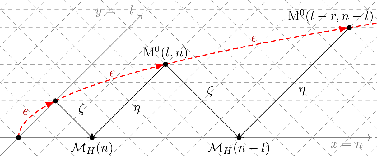
Wall-crossing alone, however, does not suffice to reveal the representation-theoretic structure of these moduli spaces, and an essentially new approach is required: we first construct the correspondences on \(\mathrm{M}^0(l,n)\) for all \(l,n\in \mathbb{Z}\), and then propagate the resulting representations to the \(\mathcal{M}_{H_\infty}(l,n)\) using the limit property and the self-similarity \(\mathrm{M}^{m}(l,n)\cong \mathrm{M}^{m-1}(l-r,n-l)\) induced by tensoring with \(\mathcal{O}_{\hat{S}}(-C)\).

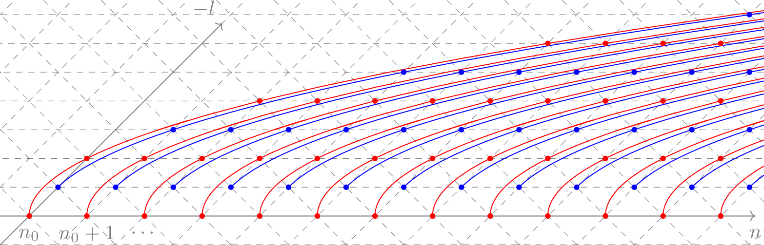
To construct the correspondences on \(\mathrm{M}^0(l,n)\), we first observe that these moduli spaces admit an explicit Grassmannian description. By [25] and [17], one has \[\label{eq:grassmannian} \mathrm{M}^0(l,n)\cong\mathrm{Gr}_{\mathcal{M}_{H}(r,c_1,n)}(\mathcal{U}_{o},-l), \quad \mathrm{M}^0(l,n)\cong \mathrm{Gr}_{\mathcal{M}_{H}(r,c_1,n-l)}(\mathcal{U}_{o}^{\vee}[1],-l),\tag{7}\] where \(\mathcal{U}_o\) is the restriction of the universal sheaf to \(\mathcal{M}_{H}(r,c_1,n)\times\{o\}\). These are precisely the two presentations appearing in the finite Clifford–Grassmannian model of Step 1, so applying 6 yields an isomorphism \[\bigoplus_{l\in\mathbb{Z}} \bigoplus_{n\in \mathbb{Z}}\mathbb{H}^*(\mathrm{M}^0(l,n))\cong \bigoplus_{l\in\mathbb{Z}} \bigoplus_{n\in \mathbb{Z}}\mathbb{H}^*(\mathrm{M}^0(l,n)) \otimes \mathrm{F}(r).\] Moreover, the embedding of the degree-\(0\) vector \(1\in \mathrm{F}(r)\) produces two additional operators \(e\) and \(f\) on \(\bigoplus_{l,n\in\mathbb{Z}}\mathbb{H}^*(\mathrm{M}^0(l,n))\). Together with the Clifford generators \(p_i,q_i\) of \(\mathrm{Cl}(r)\), these operators generate a larger algebra \(\mathcal{E}(r)\), with relations \(p_ie=0\) and \(fq_i=0\) for all \(0\leq i\leq r-1\), and \(fe=1\) and \(ef=\prod_{j=0}^{r-1}p_jq_j\).

Step 3. Morita equivalence, stable colimits, and the infinite Clifford algebra \(\mathfrak{E}(r)\). The passage from \(\mathcal{E}(r)\)-representations to representations of the infinite Clifford algebra is achieved through a Morita equivalence.

Let \(\mathfrak{E}(r)\) (defined in 6) be the infinite Clifford algebra generated by \(P_{a,i}, Q_{a,i}\), where \(a\in \mathbb{Z}, 0 \le i \le r-1\), with relations \[\{P_{a,i}, P_{b,j}\}=0,\qquad \{Q_{a,i}, Q_{b,j}\}=0,\qquad \{P_{a,i}, Q_{b,j}\}=\delta_{ij}\delta_{ab},\] and an extra invertible shift operator \(E\) satisfying \[EP_{a,i}=P_{a+1,i}E,\qquad EQ_{a,i}=Q_{a+1,i}E.\] The usual Fermionic Fock representations \(V\) are characterized by a two-sided admissibility condition: for any \(v\in V\), we have \(P_{a,i}v=0\) and \(Q_{-a,i}v=0\) for all \(a\gg 0\). For the geometric applications considered here, however, one needs a weaker one-sided (right-admissible) condition: for every vector \(v\), one only requires \[P_{a,i}v=0 \qquad \text{for all } a\gg 0.\] Perhaps unexpectedly, our algebraic result 2 establishes that the category of such representations of the infinite Clifford algebra \(\mathfrak{E}(r)\) is Morita equivalent to the category of representations of the finitely generated algebra \(\mathcal{E}(r)\).

In 29, we prove that under this Morita equivalence, the image of the \(\mathcal{E}(r)\)-module \(\bigoplus_{l,n}\mathbb{H}^*(\mathrm{M}^0(l,n))\) admits two equivalent descriptions as an \(\mathfrak{E}(r)\)-module: it is isomorphic both to \(\bigoplus_{l,n}\mathbb{H}^*(\mathcal{M}_{H_\infty}(l,n))\), and \(\bigoplus_{n} \mathbb{H}^*(\mathcal{M}_{H}(r,c_1,n))\otimes \mathfrak{F}(r)\), respectively, where \(\mathfrak{F}(r)\) is the Fermionic Fock space.

Step 4. The Boson–Fermion correspondence and the \(\hat{\mathrm{gl}}_r\)-representation. The Boson–Fermion correspondence of I. Frenkel [26] identifies the Fermionic Fock space \(\mathfrak{F}(r)\) with the basic representation of the affine Lie algebra \(\hat{\mathrm{gl}}_r\). Concretely, the affine generators are obtained from the normal-ordered quadratic fermions \[:Q_{m,i}P_{n,j}:\] Transporting, via this correspondence, the \(\mathfrak{E}(r)\)-representations of the previous step yields the desired \(\hat{\mathrm{gl}}_r\)-action on the cohomology of the blow-up moduli spaces. Moreover, restricting to the central charge-\(l\) summand gives precisely \[\bigoplus_{n\in \mathbb{Z}} \mathbb{H}^*(\mathcal{M}_{H_\infty}(l,n)) \cong \left( \bigoplus_{n\in \mathbb{Z}}\mathbb{H}^*(\mathcal{M}_{H}(r,c_1,n)) \right)\otimes \mathfrak{F}(r)_{l,\bullet},\] which is 4 . This completes the conceptual route of our proof of 1.

In this paper, the interplays between algebra and geometry are paramount. Special geometric features of the moduli spaces dictate what kind of algebra is involved. Consequently, three types of algebras appear sequentially, with one being an extension of the previous one. Representation-theoretic results of these algebras, in turn, give the anticipated topological properties of moduli spaces.

1.4 The comparison with the previous work↩︎

Since [1], [4], substantial advances have been made by both mathematicians and physicists towards understanding the relationship between the moduli space of instantons and the VOA. A pivotal first step was taken by Nakajima [20] and Grojnowski [27], who proved that the cohomology groups of the Hilbert schemes of points on an algebraic surface are the Fock space of a (super)-Heisenberg algebra. Lehn [28] constructed the Virasoro algebra, and the second-named author, Qin and Wang [29] constructed the \(W_{1+\infty}\)-algebra action on the cohomology groups of the Hilbert schemes of points on an algebraic surface.

The breakthrough on quiver varieties was also obtained by Nakajima [30], [31], where he constructed the affine Kac-Moody algebra and quantum loop algebra actions on the equivariant cohomology groups and Grothendieck groups of coherent sheaves over the Nakajima quiver varieties. Varagnolo constructed the Yangian action on the equivariant cohomology group of quiver varieties [32].

The Hilbert scheme of points is also the moduli space of rank \(1\) stable coherent sheaves on a surface. For the higher rank generalization, one of the most important advances is the Alday–Gaiotto–Tachikawa correspondence [33], which asserts that the equivariant cohomology of the moduli space of framed sheaves on \(\mathbb{P}^2\) is the Verma module of the \(W\)-algebra. It was established by Schiffmann–Vasserot [34], Maulik–Okounkov [35], and Braverman–Finkelberg–Nakajima [36]. A \(\mathrm{K}\)-theoretic generalization for any algebraic surface was developed by Negu [21].

When the assumption 1 is not satisfied, the partition function will not be the same as the generating function of the Euler characteristics of the moduli space of stable coherent sheaves, as a new contribution from the “monopole branch” will appear. When \(S\) is a projective algebraic surface, such a definition is given by Tanaka and Thomas [11], [12] using the moduli space of stable Higgs pairs. The representation theoretic explanation for the monopole branch is an interesting question, and we will pursue it in our future work.

In addition to the above novel breakthroughs, several works also directly inspired our approach. The first work is by Koseki [37], where he constructed an SOD of the derived category \(\mathrm{D}^b_{coh}(\mathcal{M}_{H_\infty}(\hat{c}))\) using a theorem of Toda [38], under a smoothness assumption. When the third-named author was working at IPMU, Nakajima suggested that the third-named author consider its relation to representation theory, which became the starting point of this paper. The results in [37] are not immediately applicable to representation theory, as the explicit Fourier–Mukai kernels by the second-named author in [39] are essential for the proof of 1, which not provided in [37], [38].

The second work is by Bershtein–Feigin–Litvinov [40], where they explained (part of) the rank \(2\) Nakajima–Yoshioka blow-up equations [41] on \(S=\mathbb{P}^2\) as an isomorphism of conformal blocks, using a different approach from ours. Their vertex algebra is the same as ours, but the conformal vector is different. To compare the different conformal vectors, one has to study the variation of Donaldson invariants under the geometric correspondences, which will be pursued in our future work.

The third work is by Diaconescu–Porta–Sala–Schiffmann–Vasserot [42], [43], where they started the study of the cohomological Hall algebra of the moduli stack of rank \(1\) coherent sheaves on a surface, and moreover related it to Yangians. While our work also involves the Hecke modification along the \((-1)\)-curve \(C\), our approach is different from theirs: the operators \(e,f\) in our paper are defined through the two Grassmannian presentations of \(\mathrm{M}^0(l,n)\), which cannot be directly obtained from the Hecke correspondences. Moreover, the limit property of \(\mathrm{M}^m(l,n)\) is an essential ingredient for the proof of 1, which also cannot be obtained solely from the Hecke correspondences.

Finally, we would like to mention the work by the third-named author [44], where he studied a toy model of the Hilbert scheme of points on the blown-up surface. Compared to [44], 1 has physical applications due to its connections with the WZW model and S-duality. From a technical point of view, the proof of 1 is also significantly more involved than that in [44] for two reasons: the Clifford algebras that act in the rank \(r\) case are more complicated than the ones that act in the rank \(1\) case, and the geometry of the correspondences is more complicated than that of [44], which we have discussed in 1.3.

1.5 The organization of the paper and some notation↩︎

In 2, we recall the moduli space of stable perverse coherent sheaves of Nakajima–Yoshioka [17]. The most technical part of our paper is proving 6 and its cohomological variants, which take up three sections from 3 to 5. From 6 to 7, we construct the \(\mathcal{E}(r)\)-action on the algebraic \(\mathrm{K}\)-theory/cohomology of the moduli space of stable perverse coherent sheaves on the blow-up. We also define the functor \(\mathfrak{H}_{\infty}\) and prove that \(\mathfrak{H}_{\infty}(\bigoplus_{l,n}\mathbb{H}^*(\mathrm{M}^0(l,n)))\) has two realizations in terms of the cohomology groups of the moduli space of coherent sheaves on blow-ups and the Fermionic Fock space, respectively. In 8, we recall the Boson–Fermion correspondence and prove the main theorem.

Let \(R\) be a unital associative algebra. We denote the opposite ring of \(R\) by \(R^{op}\) and refer to a left \(R\)-module as an \(R\)-representation. Moreover, given \(x,y\in R\), we write \([x,y]:=xy-yx\) and \(\{x,y\}:=xy+yx\). Given a finite family of elements \(\{a_i\}_{i\in S}\) in a unital ring \(R\), if \(S\) has a total order \(P\), we sort all \(a_i\) as \(a_{i_1},a_{i_2},\ldots,a_{i_{|S|}}\) such that \(i_1<_P i_2<_P \cdots <_P i_{|S|}\), and define the ordered product \[\prod_{i\in S}^{P}a_i:=\prod_{j=1}^{|S|}a_{i_j}.\]

Given any two elements \(a,b\) in a set \(S\), we use the Kronecker delta symbol \(\delta_{a,b}=1\) if \(a=b\) and \(\delta_{a,b}=0\) if \(a\neq b\).

As in 1, we use \(\mathbb{H}^*\) to denote one of the (co)homology theories, including the Grothendieck group of coherent sheaves, the Hochschild homology group, the Chow group, and the Hodge cohomology group. As in 6 , we denote the moduli space of \(d\)-dimensional quotient spaces of \(\mathbb{C}^r\) by \(\mathrm{Gr}(r,d)\).

1.6 Acknowledgments↩︎

As discussed in 1.4, we learned of this question through discussions with Hiraku Nakajima. We would like to thank him for suggesting this problem and for his valuable guidance throughout our work in this field. Y.Z. would like to thank Mikhail Bershtein, Bin Gui, Henry Liu, Andrei Neguţ, and Xin Sun for many helpful discussions and the Bernoulli Center, EPFL for the invitation to the conference "Representations, Moduli and Duality". Q. J. would also like to thank Naoki Koseki and Sasha Minets for helpful conversations. W.P. Li is supported by GRF grants 16305125 and 16306222. Q. J. was supported by the Hong Kong Research Grants Council ECS grant (Grant No. 26311724).

2 Perverse coherent sheaves on the blow-ups↩︎

In this section, we briefly review the moduli space of stable perverse coherent sheaves on the blow-up surface constructed by Nakajima–Yoshioka [17].

Let \(S\) be a smooth projective surface over \(\mathbb{C}\), with an ample divisor \(H\) and \((r,c_1)\in \mathbb{Z}_{>0}\times \mathrm{NS}(S)\) such that \(\mathrm{gcd}(r,c_1\cdot H)=1\). Let \(\mathcal{M}_{H}(n)\) be the moduli space of \(H\)-stable coherent sheaves on \(S\) with total Chern class \((r,c_1,n)\), which is a projective scheme. The universal sheaf \(\mathcal{U}\) over \(\mathcal{M}_{H}(n) \times S\), regarded as a perfect complex, is a Tor-amplitude \([0,1]\)-perfect complex of rank \(r\) (we refer to [45] and [21] for references). We fix a closed point \(o\in S\). Let \(\mathcal{U}_{o}:=\mathcal{U}|_{\mathcal{M}_{H}(n)\times \{o\}}\) be the restriction of \(\mathcal{U}\) to the fiber \(\mathcal{M}_{H}(n)\times \{o\}\).

Let \(\hat{S}:=\mathrm{Bl}_{o}S\) be the blow-up of \(S\) at \(o\) with the exceptional divisor \(C\) and the projection map \(p:\hat{S}\to S\). Then \(\mathrm{NS}(\hat{S})=p^*\mathrm{NS}(S)\oplus \mathbb{Z}[C]\) where \([C]\) is the fundamental class of \(C\) in \(\hat{S}\). For any rational number \(1\gg\epsilon>0\), \(p^*H-\epsilon C\) is \(\mathbb{Q}\)-ample. Given \(l,n\in \mathbb{Z}\), the moduli spaces of \((p^*H-\epsilon C)\)-stable coherent sheaves on \(\hat{S}\) with the total Chern class \[\label{eq:moduli} (r,p^*c_1+l[C],n-\frac{l(l+1)}{2})\in \mathbb{Z}_{>0}\times \mathrm{NS}(\hat{S})\times \mathbb{Z}\tag{8}\] are all isomorphic when \(\epsilon\) is sufficiently small, which are denoted by \(\mathcal{M}_{H_{\infty}}(l,n)\). The corresponding Chern character of 8 is \((r,p^*c_1+l[C],-n+\frac{l}{2}+\frac{c_1^2}{2})\).

Now we recall the definition of the stable perverse coherent sheaf. For any \(m\in \mathbb{Z}\), let \(\mathcal{O}_C(m):=\mathcal{O}_{\hat{S}}(-mC)|_{C}\). A coherent sheaf \(E\) on \(\hat{S}\) is called a stable perverse coherent sheaf if \(p_{*}E\) is \(H\)-stable on \(S\) with the vanishing conditions \[\operatorname{Hom}(E,\mathcal{O}_{C}(-1))=0,\quad \operatorname{Hom}(\mathcal{O}_{C},E)=0,\] and is called \(m\)-stable if \(E\otimes \mathcal{O}(-mC)\) is a stable perverse coherent sheaf. Given \(l,n\in \mathbb{Z}\), we define \(\mathrm{M}^m(l,n)\) as the moduli space of \(m\)-stable perverse coherent sheaves on \(\hat{S}\) with the total Chern class 8 .

By 2, we have \(\mathrm{M}^0(0,n)\cong \mathcal{M}_{H}(n)\) for any \(n\in \mathbb{Z}\).

3 Grassmannians of complexes and the Clifford algebra↩︎

For any integer \(r>0\), let the rank \(r\) Clifford algebra \(\mathrm{Cl}(r)\) be the unital associative \(\mathbb{Z}\)-algebra generated by elements \(p_i\) and \(q_i\) for \(i \in [r]\), subject to the relations \(p_i^2=q_i^2=0\) for all \(i \in [r]\), and \[\{p_i, p_j\} = 0, \quad \{q_i, q_j\} = 0, \quad \{p_i, q_j\} = \delta_{ij} \cdot 1 \quad \text{for all } i, j \in [r].\] Let \(\mathrm{F}(r):=\bigoplus_{d=0}^{r}\wedge^d(\mathbb{Z}^r)\) be the exterior algebra and \(\{v_i \mid i\in [r]\}\) be a standard basis of \(\mathbb{Z}^r\). Then \(\mathrm{F}(r)\) is the spin representation of \(\mathrm{Cl}(r)\) by the action \[\label{eq:rep1} p_i:=\frac{\partial}{\partial v_i}, \quad q_i:=v_i\wedge -.\tag{9}\]

In this section, we first sketch a \(\mathrm{Cl}(r)\)-action on \(\bigoplus_{d=0}^{r} \mathbb{H}^*(\mathrm{Gr}(r,d))\) for some (co)homology theory \(\mathbb{H}^*\). We only need an identification of \(\mathbb{Z}\)-modules \[\label{eq:model} \bigoplus_{d=0}^{r} \mathbb{H}^*(\mathrm{Gr}(r,d))\cong \mathrm{F}(r).\tag{10}\] We notice that the basis of \(\mathrm{F}(r)\) is parametrized by all the subsets of \([r]\), and for any \(I\subset [r]\), we define the weight and length of \(I\) as \(\mathrm{wt}(I):=\sum_{i\in I}i\) and \(\mathrm{len}(I):=\sum_{i\in I}1\). On the other hand, a partition \(\lambda\) is a sequence of positive integers \(\lambda=(\lambda_1\geq \lambda_2\geq \cdots \geq \lambda_l)\). Given any two integers \(a,b\geq 0\), let \(B_{a,b}\) be the set of partitions with \(l\leq a\) and \(\lambda_1\leq b\). By the Schubert calculus, the basis of \(\mathbb{H}^*(\mathrm{Gr}(r,d))\) can be parametrized by all partitions in \(B_{d,r-d}\). Let \(\mathrm{P}_r\) be the disjoint union of all \(B_{d,r-d}\) for \(0\leq d\leq r\). On the other hand, let \([r]:=\{0,\cdots,r-1\}\) be the set of \(r\) elements. Then 10 is naturally induced from the bijection \(\iota\) from all the subsets of \([r]\) to \(\mathrm{P}_r\) \[\begin{align} \label{eq:iotaa} \iota: (i_0<i_1<\cdots <i_{d-1})\to (i_{d-1}-d+1\geq \cdots \geq i_0). \end{align}\tag{11}\]

From 3 to 5, we generalize 10 to the Grassmannians of Tor-amplitude \([0,1]\)-complexes and also to different (co)homology theories. In particular, we construct an isomorphism of graded \(\mathrm{Cl}(r)\)-representations: \[\label{eq:once} \bigoplus_{d \in \mathbb{Z}} \mathbb{H}^*(\mathrm{Gr}_X(\mathcal{E}, d)) \cong \bigoplus_{d \in \mathbb{Z}} \mathbb{H}^*(\mathrm{Gr}_X(\mathcal{E}^{\vee}[1], d)) \otimes \mathrm{F}(r),\tag{12}\] where \(\mathbb{H}^*\) can be the Chow groups (10), Hodge cohomology groups (10), Grothendieck group of coherent sheaves (18) and Hochschild homology groups (20). The main tool for constructing 12 arises from the semi-orthogonal decomposition in derived categories, where it naturally induces a decomposition of the Grothendieck groups which is however generally not orthogonal and needs an orthogonalization procedure. Surprisingly, we find that this orthogonalization is particularly useful for constructing \(\mathrm{Cl}(r)\)-representations, which we explain in this section. We will give the geometric correspondences in 4 and 5.

3.1 The orthogonalization and \(\mathrm{Cl}(r)\)-representations↩︎

In \(\mathrm{Cl}(r)\) we define \(p_{\emptyset} = q_{\emptyset}=1\) and for any subset \(I=(a_0< \ldots< a_k) \subset [r]\) we define \[p_{I}:=p_{a_{k}}p_{a_{k-1}}\cdots p_{a_0}, \quad q_{I}:=q_{a_0}q_{a_1}\cdots q_{a_k}.\]

By 1, many properties of a \(\mathrm{Cl}(r)\)-representation \(V\) can be reduced to the computations on \(\mathrm{F}(r)\). For example, for any \(\mathrm{Cl}(r)\)-representation \(V\), we have \[\label{lem:45} (p_{[r]}q_{[r]})|_{(\cap_{i\in [r]}\mathrm{ker}(p_i))}=\mathrm{Id}, \quad (q_{[r]}p_{[r]})|_{(\cap_{i\in [r]}\mathrm{ker}(q_i))}=\mathrm{Id},\tag{14}\] and \(\sum_{I\subset [r]}q_Ip_{[r]}q_{[r]}p_I=\mathrm{Id}_V\). Regarding \(\mathrm{Cl}(r)\) as a \(\mathrm{Cl}(r)\)-representation via left multiplication, in \(\mathrm{Cl}(r)\) we have \[\label{cor:faith} \sum_{I\subset [r]}q_{I}p_{[r]}q_{[r]}p_{I}=1.\tag{15}\]

Now let \(W\) and \(V\) be two \(\mathbb{Z}\)-modules and \(\mathcal{P}\) be a total order on the set of all subsets \(I\subset [r]\). Given morphisms \(\mathfrak{e}_I:W\to V\) and \(\mathfrak{f}_I:V\to W\) for all \(I\subset [r]\), we say that they are semi-orthogonal with respect to \(\mathcal{P}\) if \[\mathfrak{f}_I\mathfrak{e}_J=\delta_{IJ} \cdot \operatorname{id}_{W} \quad \text{for all} \quad I\geq_{\mathcal{P}}J.\] We define their orthogonalization as \[\begin{gather} \label{e9} e_I:=\mathfrak{e}_I, \quad f_{I}:=\mathfrak{f}_I\prod_{J>_{\mathcal{P}}I}^{\mathcal{P}}(\mathrm{Id}_{V}-\mathfrak{e}_J\mathfrak{f}_J). \end{gather}\tag{16}\] We collect all morphisms \(e_I\) and \(f_I\) and define the morphisms \[\begin{gather} \label{eq:ehat} \hat{e}:W\otimes\mathrm{F}(r)\to V, \quad x\otimes v_I\mapsto e_Ix, \\ \nonumber \hat{f}:V\to W\otimes\mathrm{F}(r), \quad y\mapsto \sum_{I\subset [r]}f_Iy\otimes v_I. \end{gather}\tag{17}\] The surprising fact is that the morphism \(\hat{e}\) (or \(\hat{f}\)) is an isomorphism of \(\mathrm{Cl}(r)\)-representations if and only if \(\Gamma_{\mathcal{P}}:=\prod_{J\subset [r]}^{\mathcal{P}}(\mathrm{Id}_V-\mathfrak{e}_J\mathfrak{f}_J)\) acts as \(0\) on \(V\).

3.2 The dual representation and the grading↩︎

The isomorphism 17 has a duality property: let \(e_I,f_I\) satisfy the equations ?? . Then the operators \[\tilde{e}:=e_{[r]}, \quad \tilde{f}:=f_{[r]},\quad \tilde{p}_i:=q_i,\quad \tilde{q}_i:=p_i\] also satisfy ?? . Moreover, let \(\tilde{e}_I:=e_{[r]-I}\). Then \(\tilde{e}_I\) also satisfies ?? and ?? . Hence it induces another isomorphism of \(\mathrm{Cl}(r)\)-representations \[\hat{\tilde{e}}: W\otimes \mathrm{F}(r)\cong V, \quad w\otimes v_I\mapsto \tilde{e}_Iw.\] This is called the dual representation of \(V\). Moreover, \(\hat{\tilde{e}}\) is the composition of \(\hat{e}\) with the Hodge star operator: \[*: \mathrm{F}(r)\to \mathrm{F}(r), \quad v_I\mapsto s_I v_{[r]-I}.\] where \(s_I\in \{\pm 1\}\) is a sign depending on \(I\).

Now we consider the graded \(\mathrm{Cl}(r)\)-representations. The weight and length functions on the subsets \(I\subset [r]\) naturally induce the length grading and weight grading on \(\mathrm{F}(r)\). With respect to the Hodge star operator action, we define the dual length grading (resp. dual weight grading) on \(\mathrm{F}(r)\) by letting \(v_I\) have degree \(r-\mathrm{len}(I)\) (resp. \(\frac{r(r-1)}{2}-\sum_{i\in I}i\)). Given an isomorphism of representations 17 with graded \(\mathbb{Z}\)-modules \(W\) and \(V\), by direct computation we have the following condition to let 17 be an isomorphism of graded \(\mathrm{Cl}(r)\)-representations.

4 The Chow correspondences on Grassmannians of complexes↩︎

Let \(X\) be a smooth variety over \(\mathbb{C}\) and \(\mathcal{E}\) be a rank \(r\) Tor-amplitude \([0,1]\)-perfect complex. Now we state the cohomological and Chow-theoretical version of 12 . We have to impose a \(G\)-smoothness assumption, to say that \(\mathcal{E}\) is a \(G\)-smooth complex if for any \(d\geq 0\), the Grassmannians \(\mathrm{Gr}_X(\mathcal{E},d)\) and \(\mathrm{Gr}_X(\mathcal{E}^{\vee}[1],d)\) are all smooth varieties (if not empty), and their dimensions are \(\dim(X)-d(d-r)\) and \(\mathrm{dim}(X)-d(d+r)\) respectively. The complex \(\mathcal{U}_o\) over \(\mathcal{M}_{H}(n)\) under the assumption 1 is \(G\)-smooth by 4.

In 4.1, we will give the geometric correspondences. Given a class \(\alpha\in \mathrm{CH}^*(X)\), let \(\int_X \alpha\in \mathbb{Z}\) be the push-forward of \(\alpha\) to a closed point.

4.1 Geometric correspondences and the Clifford algebra action↩︎

For every rank \(n\) locally free sheaf \(E\) on \(X\), let \(c_i(E)\in \mathrm{CH}^{i}(X)\) be the \(i\)-th Chern class of \(E\) and \(c_{top}(E):=c_n(E)\) be the top Chern class. For any partition \(\lambda\), we define the Schur class \[\Delta_{\lambda}(E):= \mathrm{det}(c_{\lambda_i-i+j}(E))|_{1\leq i,j\leq l} \in \mathrm{CH}^{\mathrm{size}(\lambda)}(X),\] where \(\mathrm{size}(\lambda):=\sum_{i\in \mathbb{Z}}\lambda_i\). Given a partition \(\lambda\in B_{a,b}\) (defined in 3), the complement \(\lambda^c\) and transpose \(\lambda^t\) are defined as \[\begin{gather} \lambda^c:=(b-\lambda_a,b-\lambda_{a-1},\cdots,b-\lambda_1)\in B_{a,b},\quad \lambda^t:=(\lambda_1^t,\cdots,\lambda_b^t)\in B_{b,a}, \end{gather}\] where \(\lambda_i^t\) is the number of elements in \(\lambda\) with value \(\geq i\). We notice that \[(\lambda^t)^t=\lambda, \quad (\lambda^c)^c=\lambda, \quad (\lambda^c)^t=(\lambda^t)^c.\] We recall the bijection \(\iota\) in 11 . For any set \(I\subset [r]\), let \(I^{c}:=\{r-1-i\mid i\in I\}\) so that \(\iota(I)^c=\iota(I^c)\) for all \(I\subset [r]\) where \(b=r-d\). Under the bijection \(\iota\), the weight function satisfies \[\label{eq:weight} \mathrm{wt}(I)=\mathrm{size}(\iota(I))+\frac{\mathrm{len}(I)(\mathrm{len}(I)-1)}{2}\tag{20}\] Given integers \(a,b\geq 0\), let the partition \((a^{b})\) be \(\underbrace{(a,a,\cdots,a)}_{b \text{ times}}\).

Now we define the geometric correspondences. Let \(\mathcal{E}\) be a \(G\)-smooth complex such that \(r:=\mathrm{rank}(\mathcal{E})>0\). Given integers \(d_{-},d_+\geq 0\), we consider the incidence variety as the (classical) fiber product \[\mathrm{Inc}_{X}(\mathcal{E},d_-,d_+):= \mathrm{Gr}_X(\mathcal{E}^{\vee}[1],d_-)\times_{X}\mathrm{Gr}_X(\mathcal{E},d_+).\] By Theorem 1.3 of [47], \(\mathrm{Inc}_{X}(\mathcal{E},d_-,d_+)\) is a locally complete intersection variety and its dimension is \[\label{lem:excess} \mathrm{dim}(\mathrm{Inc}_{X}(\mathcal{E},d_-,d_+))=\mathrm{dim}(X)-d_+(d_+-r)-d_-(r+d_-)+d_+d_-\tag{21}\] For any integers \(d_-,d_+\geq 0\), let \(\mathcal{U}_+\) be the universal quotient bundle on \(\mathrm{Gr}_X(\mathcal{E},d_+)\). We consider the fundamental class of \(\mathrm{Inc}_{X}(\mathcal{E},d_-,d_+)\) in \(\mathrm{Gr}_X(\mathcal{E}^{\vee}[1],d_-)\times \mathrm{Gr}_X(\mathcal{E},d_+)\): \[\label{eq:incidence} [\mathrm{Inc}_{X}(\mathcal{E},d_-,d_+)]\in \mathrm{CH}^{\mathrm{dim}(X)-d_-d_+}(\mathrm{Gr}_X(\mathcal{E}^{\vee}[1],d_-)\times \mathrm{Gr}_X(\mathcal{E},d_+)).\tag{22}\]

The following lemma follows from direct computations:

The key point to prove 10 is the following semi-orthogonal relation, which will be proved in 4.2.

4.2 The semi-orthogonal relations↩︎

The proof of 11 is similar to [20], where the key point is a dimension estimate on the incidence varieties. First, we recall the relation between the \(G\)-smooth property and the degeneracy loci:

5 Derived Categories of Derived Grassmannians↩︎

In this section, we prove the Grothendieck group and Hochschild homology versions of 12 . The method is different from 4. The semiorthogonal decomposition of \(\mathrm{D}^b_{\mathrm{coh}}(\mathrm{Gr}_{X}(\mathcal{E}))\) established by the first-named author in [39] induces several categorical equations. By considering their decategorification, we uncover the underlying representation-theoretic structures through the lens of Clifford algebra representations.

In this section, we apply the derived algebraic geometry framework. All the categories in this section are \(\infty\)-categories and all the schemes in this section are derived schemes.

5.1 Semiorthogonal decompositions and categorical equations↩︎

We begin by describing how semiorthogonal decompositions can be expressed in terms of categorical equations.

A semiorthogonal decomposition of a stable \(\infty\)-category \(\mathcal{D}\), denoted by \[\mathcal{D} = \langle \mathcal{D}_1, \mathcal{D}_2, \ldots, \mathcal{D}_n \rangle,\] is a sequence of stable \(\infty\)-subcategories \(\mathcal{D}_1, \ldots, \mathcal{D}_n\) satisfying:

1. \(\operatorname{Hom}(D_j, D_i) \cong 0\) for all \(D_i \in \mathcal{D}_i\), \(D_j \in \mathcal{D}_j\), whenever \(j > i\).

2. For any \(D \in \mathcal{D}\), there is a sequence \[0 = D_n \to D_{n-1} \to \cdots \to D_1 \to D_0 = D\] in \(\mathcal{D}\) such that \(\mathrm{cone}(D_j \to D_{j-1}) \in \mathcal{D}_j\) for each \(1 \leq j \leq n\).

The sequence \(\mathcal{D}_1, \ldots, \mathcal{D}_n\) is called semiorthogonal if only condition (1) is required.

Now, let \(\mathcal{A}_1, \ldots, \mathcal{A}_n\) be stable \(\infty\)-categories and consider functors \[\Phi_j \colon \mathcal{A}_j \to \mathcal{D}.\] Suppose that each \(\Phi_j\) admits a left adjoint \(\Phi_j^L\). The adjunction yields natural unit and counit maps: \[\operatorname{id}_{\mathcal{D}} \to \Phi_j \Phi_j^L, \qquad \Phi_j^L \Phi_j \to \operatorname{id}_{\mathcal{A}_j}.\] Set \(\mathfrak{R}_j := \mathrm{cone}\big(\operatorname{id}_{\mathcal{D}} \to \Phi_j \Phi_j^L\big)[-1]\), the homotopy fiber of the unit map.

We now reformulate the defining conditions for a semiorthogonal decomposition in terms of the following categorical equations: \[\begin{align} \tag{26} \mathrm{cone}(\Phi_j^L\Phi_j \to \operatorname{id}_{\mathcal{A}_j}) \cong 0 \\ \tag{27} \Phi_i^L \circ \Phi_j \cong 0 \text{ for all } j>i\\ \tag{28} \mathfrak{R}_n \circ \cdots \circ \mathfrak{R}_1 \cong 0 \end{align}\]

5.2 Derived Grassmannians of perfect complexes↩︎

Next, we focus on derived Grassmannians of perfect complexes and their incidence correspondences [25], [39].

Let \(X\) be a scheme (or, more generally, a derived stack), and let \(\mathcal{E}\) be a perfect complex on \(X\) of Tor amplitude in \([0,1]\) and rank \(r \ge 0\). For an integer \(d_+ \geq 0\), we consider the (rank \(d_+\)) derived Grassmannian \[\mathrm{Gr}_X(\mathcal{E},d_+) \to X\] of the complex \(\mathcal{E}\) over \(X\) as defined in [25]. It assigns to any morphism \(T \to X\) (with \(T\) a derived scheme) the space of quotients \(\rho_+ \colon \mathcal{E}_T \twoheadrightarrow \mathcal{Q}_+\), where \(\mathcal{Q}_+\) is a vector bundle on \(T\) of rank \(d_+\), and \(\rho_+\) induces a surjection on zeroth homology. Here, \(\mathcal{E}_T\) denotes the derived pullback of \(\mathcal{E}\) to \(T\). It is a derived enhancement of the classical Grassmannian of quotients of the sheaf \(h^0(\mathcal{E})\), i.e. they have the same scheme structure, but different derived structures.

By convention, we set \(\mathrm{Gr}_X(\mathcal{E}, 0) = X\) and \(\mathrm{Gr}_X(\mathcal{E}, d_+) = \emptyset\) for \(d_+ < 0\). The projection \(\mathrm{Gr}_X(\mathcal{E},d_+) \to X\) is representable, proper, and quasi-smooth, with virtual relative dimension \(d_+(r - d_+)\) (see [25]).

The shifted derived dual \(\mathcal{E}^{\vee}[1]\) is also a perfect complex of Tor amplitude \([0,1]\), now with rank \(-r\). For any \(d_- \in \mathbb{Z}\), we similarly have the derived Grassmannian \[\mathrm{Gr}_X(\mathcal{E}^{\vee}[1],d_-) \to X,\] which is proper and quasi-smooth, with virtual relative dimension \(-d_-(r + d_-)\).

Given \(d_+, d_- \in \mathbb{Z}\), the derived incidence scheme defined in [25], \[\mathrm{Inc}_X(\mathcal{E},d_+,d_-) \to X,\] has the same underlying classical scheme as the derived fiber product \[\mathrm{Gr}_X(\mathcal{E}^{\vee}[1],d_-) \times_X \mathrm{Gr}_X(\mathcal{E},d_+),\] but with a different derived structure. Explicitly, for any \(T \to X\) (with \(T\) a derived scheme), the space of \(T\)-points of \(\mathrm{Inc}_X(\mathcal{E},d_+,d_-)\) is given by triples \[\Big(\rho_+ \colon \mathcal{E}_T \twoheadrightarrow \mathcal{Q}_+,\, \rho_- \colon \mathcal{E}_T^\vee[1] \twoheadrightarrow \mathcal{Q}_-,\, \gamma\Big),\] where \(\rho_+\) and \(\rho_-\) are \(T\)-points of \(\mathrm{Gr}_X(\mathcal{E},d_+)\) and \(\mathrm{Gr}_X(\mathcal{E}^\vee[1], d_-)\), respectively, and \(\gamma\) is a homotopy between the composition \[\mathcal{Q}_-^\vee[1] \xrightarrow{\rho_-^\vee[1]} \mathcal{E}_T \xrightarrow{\rho_+} \mathcal{Q}_+\] and zero. The “convolution" of the composition yields a canonical perfect complex \[\mathrm{cone}\Big( \mathrm{cone} \big( \mathcal{Q}_-^\vee[1] \xrightarrow{\rho_-^\vee[1]} \mathcal{E}_T\big) \xrightarrow{\rho_+} \mathcal{Q}_+ \Big)[-1] \in \mathrm{D}_{\mathrm{perf}}(T).\] This defines a universal perfect complex \[\mathcal{E}^{\mathrm{univ}}_{d_+, d_-} \in \mathrm{D}_{\mathrm{perf}}(\mathrm{Inc}_X(\mathcal{E},d_+,d_-))\] on \(\mathrm{Inc}_X(\mathcal{E},d_+,d_-)\) of Tor amplitude in \([0,1]\) and rank \(r-d_+ + d_-\).

By construction, we have a correspondence diagram \[\begin{tikzcd} & \mathrm{Inc}_X(\mathcal{E}, d_+, d_- ) \ar{dl}[swap]{r_+} \ar{dr}{r_-} & \\ \mathrm{Gr}_X(\mathcal{E}, d_+) & & \mathrm{Gr}_X(\mathcal{E}^\vee[1], d_-) \end{tikzcd}\] where the projections \(r_+\), \(r_-\), and \(\mathrm{Inc}_X(\mathcal{E},d_+,d_-) \to X\) are proper and quasi-smooth, with virtual relative dimensions \[\begin{align} d_-(d_+ - r - d_-), \quad d_+(r + d_- - d_+), \quad \text{and} \quad d_+(r - d_+) - d_-(r + d_-) + d_-d_+, \end{align}\] respectively ([39]).

5.3 Semiorthogonal decompositions and Clifford algebra representations↩︎

We now relate the semiorthogonal decompositions of derived Grassmannians to Clifford algebra representations, completing the construction of the Grothendieck group and Hochschild homology version of 12 .

Throughout, for any scheme or derived stack \(Y\), we let \(\mathrm{D}(Y)\) denote one of the following derived categories: \[\mathrm{D}_{\mathrm{qc}}(Y), \qquad \mathrm{D}^{\mathrm{b}}_{\mathrm{coh}}(Y), \qquad \mathrm{D}_{\mathrm{perf}}(Y),\] namely, the derived category of quasi-coherent sheaves, bounded coherent complexes, or perfect complexes, respectively.

Continuing with the previous subsection, we consider the unions \[\mathrm{Gr}_X(\mathcal{E}, \bullet) = \coprod_{d_+ \in \mathbb{Z}} \mathrm{Gr}_X(\mathcal{E}, d_+), \qquad \mathrm{Gr}_X(\mathcal{E}^\vee[1], \bullet) = \coprod_{d_- \in \mathbb{Z}} \mathrm{Gr}_X(\mathcal{E}^\vee[1], d_-).\] and their corresponding derived categories: \[\mathrm{D}(\mathrm{Gr}_X(\mathcal{E}, \bullet)) = \bigoplus_{d_+ \in \mathbb{Z}} \mathrm{D}(\mathrm{Gr}_X(\mathcal{E}, d_+)), \quad \mathrm{D}(\mathrm{Gr}_X(\mathcal{E}^\vee[1], \bullet)) = \bigoplus_{d_- \in \mathbb{Z}} \mathrm{D}(\mathrm{Gr}_X(\mathcal{E}^\vee[1], d_-)).\] For each \(i \in \mathbb{Z}\), we consider the incidence correspondence diagram \[\begin{tikzcd} & \mathrm{Inc}_X(\mathcal{E}, i) := \coprod_{d \in \mathbb{Z}} \mathrm{Inc}_X(\mathcal{E}, d+ i, d) \ar{dl}[swap]{r_+} \ar{dr}{r_-} & \\ \mathrm{Gr}_X(\mathcal{E}, \bullet + i) & & \mathrm{Gr}_X(\mathcal{E}^\vee[1], \bullet) \end{tikzcd}\] and the universal perfect complex \[\mathcal{E}^{\mathrm{univ}}_i = \big(\mathcal{E}^{\mathrm{univ}}_{d + i, d}\big)_{d \in \mathbb{Z}} \in \mathrm{D}_{\mathrm{perf}}(\mathrm{Inc}_X(\mathcal{E}, i))\] which has Tor amplitude in \([0,1]\) and rank \(r-i\) over \(\mathrm{Inc}_X(\mathcal{E}, i)\).

For any subset \(I \subset [r]\), write \(I = (i_0 < i_1 < \cdots < i_{j-1})\) with \(\mathrm{len}(I)=j\). We recall the associated partition \[\iota(I) := (i_{j-1} - (j-1) \geq \cdots \geq i_1 - 1 \geq i_0) \in B_{j, r-j}\] defined in 11 . Consider the Fourier–Mukai functor \[\Phi^I \colon \mathrm{D}(\mathrm{Gr}_X(\mathcal{E}^\vee[1], \bullet) \to \mathrm{D}(\mathrm{Gr}_X(\mathcal{E}, \bullet))\] which sends an object \(\mathcal{F} \in \mathrm{D}(\mathrm{Gr}_X(\mathcal{E}^\vee[1], d -r +j))\) to \[\Phi^I(\mathcal{F}) = r_{+*}\left(r_-^* (\mathcal{F}) \otimes \mathbb{S}^{\iota(I)}\big(\mathcal{E}_{r-j}^{\mathrm{univ}}\big)\right) \otimes \det(\mathcal{U}_+)^{r-j} \in \mathrm{D}(\mathrm{Gr}_X(\mathcal{E}, d)),\] where \(\mathbb{S}^{\iota(I)}(-)\) denotes the derived Schur functor ([25]), \(\mathcal{E}_{r-j}^{\mathrm{univ}}\) is the universal perfect complex on \(\mathrm{Inc}_X(\mathcal{E},r-j)\), and \(\mathcal{U}_+\) is the universal quotient bundle on \(\mathrm{Gr}_X(\mathcal{E},d)\).

By [39], the functor \(\Phi^I\) admits a left adjoint \[\Psi^I \colon \mathrm{D}(\mathrm{Gr}_X(\mathcal{E}, \bullet)) \to \mathrm{D}(\mathrm{Gr}_X(\mathcal{E}^\vee[1], \bullet)),\] which is explicitly given by a Fourier–Mukai kernel supported on \(\mathrm{Inc}_X(\mathcal{E}, r-j)\).

There is a natural lexicographic order on subsets of \([r]\): for \(I = \{i_0 < \cdots < i_{j-1}\}\) and \(J = \{k_0 < \cdots < k_{\ell-1}\}\), we write \(I <_{\mathrm{lex}} J\) if the sequence \((i_{j-1}, \ldots, i_0, -1, -1, \ldots)\) precedes \((k_{\ell-1}, \ldots, k_0, -1, -1, \ldots)\) in the usual lexicographic order. Under the bijection \(\iota: \{I|I\subset [r]\} \to \mathrm{P}_r\) from 11 , this lexicographic order \(<_{\mathrm{lex}}\) is precisely the reverse of the total order \(<\) on \(\mathrm{P}_r\) defined in [39], i.e., \(I <_{\mathrm{lex}} J\) if and only if \(\iota(I) > \iota(J)\) in \(\mathrm{P}_r\). Therefore, we have:

Consequently, for each \(d \in \mathbb{Z}\), the fully faithful functors \(\Phi^I\) induce a semiorthogonal decomposition of the degree-\(d\) component: \[\mathrm{D}(\mathrm{Gr}_X(\mathcal{E}, d)) = \left\langle \Phi^I\left(\mathrm{D}\big(\mathrm{Gr}_X(\mathcal{E}^\vee[1],\, d - r + \mathrm{len}(I))\big)\right) \;\middle|\; I \subset [r] \right\rangle.\]

A parallel result holds for Hochschild homology

6 Perverse stable sheaves on blow-ups, the extended algebra \(\mathcal{E}(r)\) and the Morita equivalence↩︎

Now we recall \(\mathrm{M}^0(l,n)\) from 2. For any \(n,l\in \mathbb{Z}\), by 2, we have isomorphisms \[\mathrm{M}^0(l,n)\cong \mathrm{Gr}_{\mathcal{M}_H(n)}(\mathcal{U}_o,-l), \quad \mathrm{M}^0(l,n+l)\cong \mathrm{Gr}_{\mathcal{M}_H(n)}(\mathcal{U}_o^{\vee}[1],-l).\] By 18 and 7, for any \(n\in \mathbb{Z}\), we have a \(\mathrm{Cl}(r)\) action on \(\oplus_{n\in \mathbb{Z}} \mathbb{H}^*( \mathrm{M}^0(l,n))\) and maps \[\begin{align} e:\mathbb{H}^*(\mathrm{M}^0(l+r,n+l+r))\to \mathbb{H}^*(\mathrm{M}^0(l,n)), \\ f:\mathbb{H}^*(\mathrm{M}^0(l,n))\to \mathbb{H}^*(\mathrm{M}^0(l+r,n+l+r)) \end{align}\] such that ?? holds. Thus \(e,f\) induce endomorphisms on \(\bigoplus_{l,n\in \mathbb{Z}} \mathbb{H}^*(\mathrm{M}^0(l,n))\). Let \(\mathcal{E}(r)\) be the extended algebra over \(\mathrm{Cl}(r)\) with two additional elements \(e\) and \(f\) with the relations ?? \[p_{i}e=0, \quad fq_{i}=0, \quad fe=1, \quad ef=p_{[r]}q_{[r]}.\] Then by the above explanation, the algebra \(\mathcal{E}(r)\) naturally acts on \[\label{eq:act} \mathcal{E}(r) \curvearrowright \bigoplus_{l,n\in \mathbb{Z}}\mathbb{H}^*(\mathrm{M}^0(l,n)).\tag{29}\]

On the other hand, we can also obtain \(\mathcal{E}(r)\) through the Morita theory: let the infinite-dimensional Clifford algebra \(\mathfrak{E}(r)\) be the unital algebra generated by elements \(P_{a,i}, Q_{a,i}, a\in \mathbb{Z}, i\in [r]\) and an invertible element \(E\) with the relations \[\label{eq:clifford} \begin{align} P_{a,i}^2=0, \quad Q_{a,i}^2=0, \quad EP_{a,i}=P_{a-1,i}E, \quad EQ_{a,i}=Q_{a-1,i}E \quad \text{ for all } a,i\\ \{P_{a,i}, P_{b,j}\}=0, \quad \{Q_{a,i}, Q_{b,j}\}=0, \quad \{P_{a,i}, Q_{b,j}\}=\delta_{ij}\delta_{ab} \quad \text{for all a,b,i,j,} \end{align}\tag{30}\] Let \(F:=E^{-1}\). In this section, we will prove that

Let \(\mathrm{Mod}_0\) (resp. \(\mathrm{Mod}_{\infty}\)) be the abelian category of left \(\mathcal{E}(r)\)-modules (resp. left \(\mathfrak{E}(r)\)-modules). By the Morita theory (see Theorem 2.5 of [54]), there is a Morita equivalence between \(\mathrm{Mod}_0\) and \(\mathrm{Mod}_{\infty}^R\) by the functors: \[\begin{align} \mathfrak{H}_{\infty}: \mathrm{Mod}_0 &\to \mathrm{Mod}_{\infty}, \quad V\mapsto \Lambda_{r}\otimes_{\mathcal{E}(r)}V, \\ \mathcal{H}_0: \mathrm{Mod}_{\infty} &\to \mathrm{Mod}_0, \quad W\mapsto \mathrm{Hom}_{\mathfrak{C}(r)}(\Lambda_{r},W). \end{align}\]

6.1 The bimodule structure↩︎

We first give the definition of admissible left \(\mathfrak{E}(r)\)-modules. For any \(I=(d_0<d_1<\cdots<d_k)\subset [r]\) and \(a,b\in \mathbb{Z}\), let \[P_{a,I}:=P_{a,d_{k}}P_{a,d_{k-1}}\cdots P_{a,d_0},Q_{b,I}:=Q_{b,d_{0}}Q_{b,d_{1}}\cdots Q_{b,d_k}.\] For \(V\in \mathrm{Mod}_\infty\), let \[\begin{gather} \mathcal{H}_m(V):=\bigcap_{a> m, i\in [r]} \ker(P_{a,i}), \quad \mathcal{K}_m(V):=\bigcap_{a\leq m, i\in [r]} \ker(Q_{a,i}). \\ \quad \mathcal{H}_{\infty}(V):=\bigcup_{m\in \mathbb{Z}}\mathcal{H}_m(V),\quad \quad \mathcal{K}_{-\infty}(V):=\bigcup_{m\in \mathbb{Z}}\mathcal{K}_m(V). \end{gather}\] We notice that \(\mathcal{H}_{\infty}(V)\) and \(\mathcal{K}_{-\infty}(V)\) are also \(\mathfrak{C}(r)\) sub-representations of \(V\). The representation \(V\) is defined to be right admissible (resp. left admissible, admissible) if \(\mathcal{H}_{\infty}(V)=V\) (resp. \(\mathcal{K}_{-\infty}(V)=V\), \(\mathcal{H}_{\infty}(V)\cap\mathcal{K}_{-\infty}(V)=V\)). Let \(\mathrm{Mod}_{\infty}^{R}\) be the full subcategory of \(\mathrm{Mod}_{\infty}\) consisting of right admissible representations.

Before proving 22, we give the following corollary, which describes the functors \(\mathcal{H}_0\) and \(\mathfrak{H}_{\infty}\) explicitly.

The key to proving 22 is the identification of \(\Lambda_r\) and \(\Lambda_{\infty,r}\) as an \(\mathfrak{E}(r)\)-\(\mathcal{E}(r)\) bimodule.

6.2 A precise formulation of 29↩︎

Now we give a precise formulation of 29 and its cohomological variants. In particular, we formulate the degree shift of the action under different gradings, which can be obtained through direct computations.

7 The admissible representation of \(\mathfrak{C}(r)\) and the colimit↩︎

In this section, we study the image of \(\bigoplus_{l,n}\mathbb{H}^*(\mathrm{M}^0(l,n))\) under the functor \(\mathfrak{H}_{\infty}\). In particular, we need to prove the following two isomorphisms \[\begin{align} \label{stable:limit} \mathfrak{H}_{\infty}(\bigoplus_{l,n}\mathbb{H}^*(\mathrm{M}^0(l,n)))\cong \bigoplus \mathbb{H}^*(\mathcal{M}_{H_{\infty}}(l,n)), \\ \nonumber \mathfrak{H}_{\infty}(\bigoplus_{l,n}\mathbb{H}^*(\mathrm{M}^0(l,n)))\cong \bigoplus_{n\in \mathbb{Z}}\mathbb{H}^*(\mathcal{M}_{H}(n))\otimes \mathfrak{F}(r), \end{align}\tag{41}\] as \(\mathbb{Z}\)-modules and \(\mathfrak{E}(r)\)-representations respectively, where we define the Fermionic Fock space \(\mathfrak{F}(r)\) in a way compatible with our geometric correspondences:

7.1 The admissible representations↩︎

The \(\mathrm{Cl}(r)\)-representation on \(\mathrm{F}(r)\) in 9 induces a natural \(\mathfrak{E}(r)\)-representation on \(\mathfrak{F}(r)\) where \(Ev_{\mathfrak{I}}:=v_{\mathfrak{I}^-}\), \(Fv_{\mathfrak{I}}:=v_{\mathfrak{I}^+}\) such that the \(i\)-th term of \(\mathfrak{I}^{\pm}\) is defined as the \((i\mp 1)\)-th term of \(\mathfrak{I}\) and \[\begin{align} P_{a,i}v_{\mathfrak{I}}:= (-1)^{\sum_{k>a}\mathrm{len}(I_k)}\cdots \otimes v_{I_{a-1}}\otimes (p_{i}v_{I_{a}}) \otimes v_{I_{a+1}} \cdots, \\ Q_{a,i}v_{\mathfrak{I}}:= (-1)^{\sum_{k>a}\mathrm{len}(I_k)}\cdots \otimes v_{I_{a-1}}\otimes (q_{i}v_{I_{a}}) \otimes v_{I_{a+1}} \cdots. \end{align}\] Moreover, given an automorphism \(T\) on a \(\mathbb{Z}\)-module \(W\), \(\mathfrak{F}(W,T) := W\otimes \mathfrak{F}(r)\) has a canonical \(\mathfrak{C}(r)\)-action by \[\begin{align} E(w\otimes v_{\mathfrak{I}}):=T(w)\otimes v_{\mathfrak{I}^{-}}, \quad F(w\otimes v_{\mathfrak{I}}):=T^{-1}(w)\otimes v_{\mathfrak{I}^+}, \\ P_{l,i}(w\otimes v_{\mathfrak{I}}):=w\otimes P_{l,i}v_{\mathfrak{I}}, \quad Q_{l,i}(w\otimes v_{\mathfrak{I}}):=w\otimes Q_{l,i}v_{\mathfrak{I}}. \end{align}\] We prove that any admissible \(\mathfrak{C}(r)\)-representation is of the form \(\mathfrak{F}(W,T)\).

7.2 Bounded bigraded \(\mathcal{E}(r)\)-representations and the parabolic colimit↩︎

For a \(r\)-Maya diagram \(\mathfrak{I}\), we define the central charge and the weight as \[\begin{align} c_{\mathfrak{I}}:=\sum_{l\in \mathbb{Z}_{>0}}\mathrm{len}(I_l)-\sum_{l\in \mathbb{Z}_{\leq 0}}(r-\mathrm{len}(I_l)), \\ w_{r,\mathfrak{I}}:=\sum_{l\in \mathbb{Z}_{>0}}l\cdot \mathrm{len}(I_l)-\sum_{l\in \mathbb{Z}_{\leq 0}}l(r-\mathrm{len}(I_l)). \end{align}\] They induce a bigrading on \(\mathfrak{F}(r)\) by \[\mathfrak{F}(r)=\bigoplus_{l,m\in \mathbb{Z}}\mathfrak{F}(r)_{l,m}, \quad \mathfrak{F}(r)_{l,m}=\langle v_{\mathfrak{I}}|c_\mathfrak{I}=l, w_{r,\mathfrak{I}}=m\rangle.\]

Let \(\mathfrak{F}(r)^{\leq 0}:= \mathcal{H}_0(\mathfrak{F}(r))\), which is the free \(\mathbb{Z}\)-module generated by all Maya diagrams \(\mathfrak{I}\) such that \(I_{m}=\emptyset\) for all \(m>0\). There is a canonical bigraded \(\mathcal{E}(r)\)-action on \(\mathfrak{F}(r)^{\le 0}\) induced from the functor \(\mathcal{H}_0\). By direct computation, the operators \(p_{0,i},q_{0,i},e,f, e_{[r]},f_{[r]}\) shift the central charge degree and the weight degree on \(\mathfrak{F}(r)^{\leq 0}_{l,\bullet} = \bigoplus_{m \in \mathbb{Z}} \mathfrak{F}(r)_{l,m}^{\le 0}\), respectively, by \[\begin{gather} \label{lem:grading} -1,1,-r,r,0,0, \text{ and } 0,0,-l,l+r,l,-l, \end{gather}\tag{42}\] which is similar to the degree shift in 23 and 24. Moreover, for any \(l>0\), we have \(\mathrm{G}_0(\mathrm{M}^0(l,n))=0\) for all \(n\in \mathbb{Z}\) by 2 and \(\mathfrak{F}(r)_{l,n}^{\leq 0}=0\) by the definition of central charge. Given \(n\ll 0\), by the Bogomolov–Gieseker inequality (and also 2) and the definition of the weight, we have \(\mathrm{G}_0(\mathrm{M}^0(l,n))=0\) and \(\mathfrak{F}(r)_{l,n}^{\leq 0}=0\) for all \(l\in \mathbb{Z}\). We summarize the above similarities to give the definition of a bounded bigraded \(\mathcal{E}(r)\)-representation:

Given a bounded bigraded \(\mathcal{E}(r)\)-representation \(V\), the operator \(E,F,P_{0,i},Q_{0,i}\) shift the central charge degree and weight degree by \(-r,r,-1,1\) and \(-l,l+r,0,0\) on \(\mathfrak{H}_{\infty}(V)_{l,n}\) respectively.

7.3 The verification of 41↩︎

Now we verify 41 and its cohomological variants. Due to the rigidity of 27, we can prove much stronger statements.

To formulate the cohomological variants of 29, we need to define a cohomological grading on \(\mathfrak{F}(r)\) such that the operators \(p_{0,i},q_{0,i},e,f,e_{[r]},f_{[r]}\) on \(\mathfrak{F}(r)^{\leq 0}\) shift the cohomological grading by \[i,-i,-rl+\frac{1}{2}r(r-1),r(l+r)-\frac{1}{2}r(r-1),lr,-lr,\] which matches the degree shift in 10. The grading is given by \[\label{coho} \mathrm{coho}_{\mathfrak{I}}:=\sum_{m\in \mathbb{Z}_{\leq 0}}(\frac{r(r-1)}{2}-\mathrm{wt}(I_m))-\sum_{m\in \mathbb{Z}_{>0}}\mathrm{wt}(I_m)+rw_{r,\mathfrak{I}}.\tag{44}\] for any \(r\)-Maya diagram \(\mathfrak{I}\). The proof of the following argument is similar to 29.

8 The proof of main theorems and the Boson–Fermion correspondence↩︎

Now we state our main theorems. We follow the notations in 7 for the representation theory and 2 for the moduli space of stable coherent sheaves and assume that \(\mathrm{gcd}(r,c_1\cdot H)=1\). Given \(r>0\), the affine Lie algebra \(\hat{\mathrm{gl}}_r\) is defined by the generators \(e_{ij}^{m}, m\in \mathbb{Z}, i,j\in [r]\), central element \(K\) and a derivation \(d\) such that \[\begin{gather} \tag{45} [e_{ij}^a, e_{kl}^b]=(\delta_{jk}e_{il}^{a+b}-\delta_{il}e_{kj}^{a+b})+a\delta_{il}\delta_{jk}\delta_{a,-b}K, \\ \tag{46} [d, e_{ij}^{l}]=l e_{ij}^{l}, \quad [d,K]=0. \end{gather}\]

We notice that 47 and 48 have been proved as isomorphisms of \(\mathfrak{C}(r)\)-representations in 29 30. The remaining step is to induce the \(\hat{\mathrm{gl}}_r\)-representation from the \(\mathfrak{C}(r)\) action. This is the famous Boson–Fermion correspondence of I. Frenkel [26], where the Fermionic Fock space \(\mathfrak{F}(r)\) can also be decomposed as the direct sum of basic representations of \(\hat{\mathrm{gl}}_r\) with different central charges:

9 Visualizations of bounded bigraded \(\mathcal{E}(r)\)-representations↩︎

This appendix presents visualizations of bounded bigraded \(\mathcal{E}(r)\)-representations \[V=\bigoplus_{l\le 0,\; n\in\mathbb{Z}} V_{l,n},\] in 7.2 by placing the graded pieces on the affine \((n,-l)\)-plane and tracing the parabolic trajectories generated by the \(e\)-action, with particular attention to the geometric case \(V_{l,n}=\mathbb{H}^*(\mathrm{M}^0(l,n))\).

9.1 The affine \((n,-l)\)-plane↩︎

Let \(\mathrm{M}^0(l,n)\) denote the moduli of stable perverse coherent sheaves from 2. Then each \(\mathrm{M}^0(l,n)\) fits into a diagram \[\begin{tikzcd}& \mathrm{M}^0(l,n) \arrow[dl, "\eta"'] \arrow[dr, "\zeta"] & \\ \mathcal{M}_H(n) & & \mathcal{M}_H(n-l) \end{tikzcd}\] where \(\eta\) and \(\zeta\) are Grassmannian of rank \((-l)\) associated to the complexes \(\mathcal{U}_0\) and \(\mathcal{U}_0^\vee[1]\) (see 2). We visualize all the moduli spaces \(\mathrm{M}^0(l,n)\) by placing each \(\mathrm{M}^0(l,n)\) at the lattice point on the affine \((x,y) = (n,-l)\)-plane as in Figure 1; lattice points on the \(n\)-axis precisely correspond to \(\mathrm{M}^0(0,n)=\mathcal{M}_H(n)\).

With this coordinate choice (so the \(-l\)-direction appears at \(45^\circ\)), the diagonal arrows record the geometric maps: the left-down \(45^\circ\) arrow from \((n,l)\) to \((n,0)\) represents \(\eta\), and the right-down \(45^\circ\) arrow from \((n,l)\) to \((n-l,0)\) represents \(\zeta\).

9.2 Parabolic trajectories of the \(e\)-action↩︎

More generally, let \[V=\bigoplus_{l \le 0,\; n\in\mathbb{Z}} V_{l,n}\] be a bigraded \(\mathcal{E}(r)\)-representation as in 7. We can similarly visualize \(V\) by placing each \(\mathbb{Z}\)-module \(V_{l,n}\) at the lattice point on the affine \((n,-l)\)-plane, as in Figure 1. Iterating the action of \(e\in\mathcal{E}(r)\) then produces \[V_{l,n}\xrightarrow{e}V_{l-r,\,n-l}\xrightarrow{e}V_{l-2r,\,n-2l+r}\xrightarrow{e}\cdots \xrightarrow{e} V^{(m)}_{l,n}\xrightarrow{e} V^{(m+1)}_{l,n}\xrightarrow{e}\cdots,\] where \[V^{(m)}_{l,n}:=V_{\,l-mr,\; n-ml+\tfrac{m(m-1)}{2}r}\] corresponds to \(t^m V(l,n)\) from 3. Thus the orbit \[\mathbb{O}(l,n):=\{\,V^{(m)}_{l,n}\mid m \in \mathbb{Z}_{\ge 0} \,\}\] is represented by the sequence of lattice points lying on the parabola \[(x-n)=\frac{1}{2r}\,(y+l)\,(y-r-l)\] in the \((x,y)=(n,-l)\)-plane; see Figure 1. We call such a sequence \(\mathbb{O}(l,n)\) a parabolic trajectory. Note that the parabolic trajectories \(\mathbb{O}(l,n)\) and \(\mathbb{O}(-r-l,n)\) lie on the same parabola, but they are disjoint unless \(l\equiv -r-l\pmod r\).

Every \(\mathbb{Z}\)-module \(V_{l',n'}\) lies on a unique trajectory \(\mathbb{O}(l, n)\) with \(1-r\le l \le 0\) and \(n\in\mathbb{Z}\), and distinct trajectories \(\mathbb{O}(l, n)\) with \(1\!-\!r\le l\le 0\) are disjoint. Hence the lattice labeled by \(V_{l,n}\) is foliated by the parabolic trajectories \(\mathbb{O}(l,n)\), indexed by \(n\in\mathbb{Z}\) and \(1-r\le l\le 0\).

In the geometric situation where \(V_{l,n}=\mathbb{H}^* (\mathrm{M}^0(l,n))\), the Bogomolov–Gieseker inequality yields boundedness: there exists \(n_0\) such that \(V_{l,n}=0\) for all \(n<n_0\). Moreover, the Chern class of the sheaves parametrized by \(\mathrm{M}^0(l,n)\) satisfy the Bogomolov–Gieseker inequality if and only if the Chern class of the sheaves parametrized by \[\mathrm{M}^m(l,n)\cong \mathrm{M}^0\!\big(l-mr,\; n-ml+\tfrac{m(m-1)}{2}\,r\big)\] does. Consequently, the potentially nonempty moduli \(\mathrm{M}^0(l,n)\) occur precisely at lattice points lying on the parabolic trajectories \(\mathbb{O}(l,n)\) with \(n\ge n_0\) and \(1-r\le l\le 0\); see 2 for an illustration when \(r=2\).

9.3 The \(\mathcal{E}(r)\)-action↩︎

The actions of \(e\) (and hence \(f\)) are shown in Figures 1 and 2. In particular, \(e\) moves forward along each parabolic trajectory \(\mathbb{O}(l,n)\), while \(f\) moves backward. In these figures, the family of operators \(q_{a,i}\) with \(a\le 0\) from 36 can be depicted as follows, exhibiting a pattern similar to differentials on successive pages of a spectral sequence: \[\begin{figure}\includegraphics[width=0.8\textwidth]{_pdflatex/lgveixrf.png}\label{hdazywnu}\end{figure}\tag{49}\] The operators \(p_{a,i}\) act in the directions opposite to the corresponding \(q_{a,i}\).

9.4 Stable colimits and \(\mathfrak{E}(r)\)-action↩︎

By 27, if \(V\) is a bounded bigraded \(\mathcal{E}(r)\)-representation, then each parabolic trajectory \(\mathbb{O}(l,n)\) stabilizes after finitely many steps: \[\mathfrak{H}_{\infty}(V)_{l,n} \cong V_{l,n}^{(m)} \quad \text{for all } m \gg 0.\] In the geometric setting \(V_{l,n}=\mathbb{H}^*(\mathrm{M}^0(l,n))\), 29 identifies the stable colimit as \(\mathfrak{H}_{\infty}(V)_{l,n} = \mathbb{H}^*(\mathcal{M}_{H_\infty}(l,n)).\)

In the colimit \(\mathfrak{H}_{\infty}(V)\), the operator \(e\) is (formally) invertible, so each stabilized parabolic orbit as in Figure 2 extends to the negative direction \(\{\mathfrak{H}_{\infty}(V)_{l,n}^{(m)}\}_{m\in\mathbb{Z}}\), and all transition maps along the orbit are isomorphisms. The operators \(E\) and \(F\) move forward and backward, respectively, along each stabilized parabolic orbit. Moreover, the operators \(p_{a,i}\) and \(q_{a,i}\) for \(m \le 0\) descend to well-defined operators \(P_{a,i}\) and \(Q_{a,i}\) on the colimit. Similar to \(q_{a,i}\), the operators \(Q_{a,i}\) for \(a \ge 0\) can be visualized as follows: \[\begin{figure}\includegraphics[width=0.8\textwidth]{_pdflatex/qlcgerft.png}\label{ksfpxlaj}\end{figure}\tag{50}\] The operators \(P_{a,i}\) act in the directions opposite to the corresponding \(Q_{a,i}\).

References↩︎