FUSE: A Flow-based Mapping Between Shapes
November 17, 2025
Abstract
We introduce a novel neural representation for maps between 3D shapes based on flow-matching models, which is computationally efficient and supports cross-representation shape matching without large-scale training or data-driven procedures. 3D shapes are represented as the probability distribution induced by a continuous and invertible flow mapping from a fixed anchor distribution. Given a source and a target shape, the composition of the inverse flow (source to anchor) with the forward flow (anchor to target), we map points between the two surfaces. By encoding the shapes with a pointwise task-tailored embedding, this construction provides an invertible and modality-agnostic representation of maps between shapes across point clouds, meshes, signed distance fields (SDFs), and volumetric data. The resulting representation consistently achieves high coverage and accuracy across diverse benchmarks and challenging settings in shape matching. Beyond shape matching, our framework shows promising results in other tasks, including UV mapping and registration of raw point cloud scans of human bodies.
1 Introduction↩︎
Shape matching has long been recognized as a “key problem” in geometry processing: indeed, accurate correspondences between two shapes enable simple solutions for several downstream tasks (, pose transfer [1] or interpolation [2]). Most of the research in this field, following the common practices from 3D graphics industry, was built on the triangle mesh representation, which approximates a continuous 2-dimensional manifold embedded in \(\mathbb{R}^3\) piecewise linearly with a collection of triangles connected by their common edges and vertices. However, recent progress in the fields of computer vision and deep learning has popularized novel ways of encoding 3D geometry, such as neural representations [3], [4]. These solutions offer several advantages compared to triangle meshes, but lack their large suite of tools and algorithms for analysis and manipulation [5].
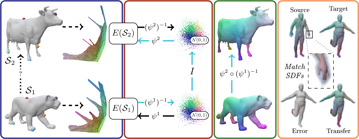
In this work, we address this challenge by introducing a novel representation for maps between a source and a target shape that can be applied over various geometric encodings. We namely refer to this representation as FUSE. Constructing a map with this representation requires only two components: i) the ability to sample points from the involved surfaces, and ii) a pointwise feature embedding designed for the target task. Once feature embeddings are computed for the sampled points on both source and target shapes, FUSE estimates an invertible flow from each embedding distribution to a shared anchor distribution, following Flow Matching framework [6]. FUSE then expresses the map between the two shapes as the composition of the inverse flow of the source (source \(\to\) anchor) and the forward flow of the target (anchor \(\to\) target). We note that, given the flows of any two shapes, the map is obtained with no additional optimization, with only landmarks as information shared by the two shapes.
In the context of shape matching, our representation introduces a probabilistic perspective on embedding alignment, where semantically similar features are encouraged to align through a shared probability distribution. Combined with the guarantee of mapping points directly into the target embedding space, our framework produces high-coverage and accurate correspondences that are relevant for different applications. We evaluate the proposed approach through a comprehensive experimental study, comparing it against several shape matching baselines, ranging from well-established axiomatic methods to recent data-driven approaches; FUSE shows high, if not the highest, accuracy on various benchmarks. Our contributions can be summarized as follows:
We introduce FUSE, the first flow-matching based representation for 3D shape maps that naturally enables correspondence between shapes expressed in different modalities (e.g., meshes, point clouds, and SDFs);
We quantitatively show that FUSE achieves competitive or superior matching accuracy over state-of-the-art methods, particularly in the context of landmark-based shape matching;
We showcase the versatility of FUSE, employing it as a backbone for other downstream applications, ranging from shape parametrization to point cloud deformation.
2 Related Work↩︎
2.1 Neural Shape Representations↩︎
Recent research in geometric deep learning and geometry processing popularized the practice of encoding 3D shapes in the weights of neural networks, which is referred to as neural shape representation. The early contributions in this field are due to [7] and [3], followed by the introduction of NeRF [4], which led to a vast effort to adapt neural shape representations to other tasks besides reconstruction. Examples of these adaptations are to shape deformation [5], [8]–[10], text-guided shape editing [11], [12] and generation [13], [14]. Recent contributions also introduced neural representations for 3D simulations [15] and computation of geometric operators over spherical neural surfaces [16].
The work of [17] is closely related to ours, as they propose a method to represent functions continuously over surfaces in intrinsic space. Lastly, FUSE’s architecture is inspired by Geometry Distributions [18], which proposes to represent geometry as a continuous map from a 3D Gaussian distribution to the surface with a denoising diffusion model [19]. However, by targeting the specific goal of representing maps between shapes, we build upon flow matching [6], and model flows directly over an intrinsic feature space, rather than standard Euclidean or extrinsic coordinates. These two choices together enable FUSE to represent mappings, as we prove by targeting the shape correspondence task.
2.2 Shape Matching↩︎
Shape correspondence is a fundamental task in geometry processing, with a wide range of approaches proposed over the years, which can largely be distinguished by how they represent the map between shapes and features [20]–[24]. Among these, the functional map framework [25] and its follow-up works [26]–[30] have emerged as a dominant paradigm, where correspondences are represented as linear operators between functional spaces. These methods offer attractive properties such as smoothness and invariance to deformations, but the reliance on spectral bases limits their generalization to non-mesh representations [27] and in obtaining bijective maps [31]–[33].
Another class of approaches leverages optimal transport (OT) [34]–[36], in which correspondences are represented by transport plans that minimize the cost of transporting a distribution of features from one shape to another. In the presence of sampling imbalances or ambiguous features, OT plans often exhibit mass-splitting behavior, where individual points distribute probability mass across multiple targets. This diffusion can degrade correspondence sharpness and stability when recovering discrete maps. Alternatively, registration-based approaches directly optimize non-linear deformation fields in 3D [2], [37]–[39]. The fields are often parameterized via deformation networks or complex architectures, achieving accurate alignments at the cost of solving computationally heavy optimization problems and depending on rigid initialization or learned priors.
Hybrid approaches combine the strengths of the above formulations [29], [40]–[45], gaining in efficiency and robustness, but still relying on learned priors and struggling to generalize to other representations. Another common approach is template-based matching, representing correspondences as a composition of maps with respect to a common template, selected a priori [46]–[48] or directly at test time [49]. On a different perspective, FUSE offers a novel representation for maps. Based on flow matching [6], our method models a correspondence as a composition of continuous invertible flows between intrinsic feature spaces and a shared anchor distribution, inherently enforcing bijectivity and high-coverage in obtained maps, without learned priors or per-pair optimization in a pipeline naturally agnostic of the geometric representation.
3 Background↩︎
3.0.0.1 Shapes and Matching.
A 3D shape \(\mathcal{S}\) is modeled as a compact two-dimensional manifold embedded in \(\mathbb{R}^3\). From a computational standpoint, single shapes may be represented in several ways: polygonal meshes, point clouds, signed distance functions and volumetric meshes are notable examples. In this work, we identify a shape \(\mathcal{S}\) as a continuous manifold from which we can sample unordered sets of points \(\{x_i\}_{i=0}^{n}\), encoded by their 3D coordinates (i.e. \(x_i \in \mathbb{R}^3\)) independently from the adopted representations.
Given 3D shapes \(\mathcal{S}_1=\{x_{i}\}_{i=1}^{n_1}\) and \(\mathcal{S}_2=\{y_{j}\}_{j=1}^{n_2}\) with a common semantic, a point-to-point correspondence \(T_{12}\) maps each point \(x_i\) to its corresponding point \(y_j\). Shape matching is the task of estimating such correspondence. In the non-rigid scenario, estimating correspondences directly from 3D coordindates is challenging; thus, most methods describe the shapes via pointwise features, characterizing their semantics and geometry [20], [22], [50]. For each point \(x_i \in \mathcal{S}_1\), we compute a vector of features \(f_i\in \mathbb{R}^{d}\) that we can then store as a row in the embedding matrix \(E_1\in \mathbb{R}^{n_1\times d}\) (same goes for \(\mathcal{S}_2\)). Ideally, one can solve for the correspondence directly by leveraging the similarity between these encodings [21]. In practice, more complex pipelines are required to align the features and retrieve the correspondence from their relations [25].
3.0.0.2 Flow Matching.
Flow Matching (FM) [6], [51] is a framework for learning continuous in time probability paths \((p_t)_{t \in [0,1]}\) that transport a known source distribution \(p_0\) (, a Gaussian) to an unknown target \(p_1\) (, data samples). This is achieved by learning a velocity field \(u_t^\theta(x)\) describing the instantaneous dynamics of the path, parameterized by a neural network \(\theta\). For each \(x \in \mathbb{R}^d\), the velocity field induces a flow \(\psi_t(x)\) as the solution of the ODE \(\frac{d}{dt}\psi_t(x) = u_t(\psi_t(x))\) with initial condition \(\psi_0(x) = x\). Crucially, the flow \(\psi_t\) is invertible and diffeomorphic: starting from any point sampled from \(p_1\), i.e., \(x \sim p_1\), integrating the ODE backward yields a point \(\psi^{-1}_0(x) \sim p_0\). The bidirectionality enables transport between distributions in both directions. Since \(u_t\) is generally intractable, [6], [51] proposed Conditional Flow Matching (CFM), replacing \(u_t\) with a tractable conditional velocity field \(u_t(x_t \mid x_1)\), while preserving the same gradients: \[\mathcal{L}_{\text{CFM}}(\theta) = \mathbb{E}_{t, x_1, x_t \sim p_t(\cdot|x_1)} \left[ \lVert v^\theta_t(x_t) - u_t(x_t \mid x_1)\rVert^2 \right].\] where \(\mathbb{E}_{t, x_1, x_0}\) represents the average over randomly sampled timesteps in \([0,1]\) and over source and target samples \(x_0 \sim p_0,x_1 \sim p_1\). A simple choice for the field is linear interpolation, \(x_t = (1-t)x_0 + t x_1\) with \(u_t = x_1 - x_0\). CFM training is thus simulation-free, although generating samples still requires integrating the learned ODE. In the remainder of the paper, we will refer to CFM simply as Flow Matching (FM).
4 FUSE↩︎
Given the overview presented in the previous section, we can now provide all the details of our novel representation FUSE which we outlined in 1. The complete source code is available at https://github.com/LorenzoOlearo/FUSE-Flow-based-Mapping-Between-Shapes.
4.1 Flow Optimization↩︎
Given a pair of shapes \(\mathcal{S}_1=\{x_{i}\}_{i=1}^{n_1}\), \(\mathcal{S}_2=\{y_{j}\}_{j=1}^{n_2}\) and an embedding matrix \(E_\ell\in \mathbb{R}^{n_\ell\times d}\) (with \(\ell =1\) or \(2\)), we denote the resulting embedding distributions as \(p^{\ell} = E_{\ell}\) (see blue box of 1). For each shape, we train an independent flow model that learns a continuous, invertible mapping \(\psi^{\ell}\colon[0,1]\times\mathbb{R}^d\to\mathbb{R}^d\). This flow transports samples from a fixed, shared Gaussian \(p_0 = \mathcal{N}(0,1)^d\) (the anchor distribution) to the shape’s embedding distribution \(p^{\ell}\), i.e. \(\psi^{\ell}_1(x) \sim p^{\ell}\) given \(x\sim p_0\). Each flow is parametrized by a neural network and trained via Conditional Flow Matching [6], [51] as we described earlier (see red box of 1). Each flow is trained independently on its shape, requiring only the ability to sample embeddings from the surface.
4.2 Fusing Representations↩︎
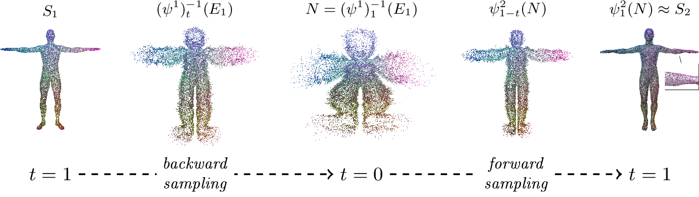
FUSE determines maps between shapes by composing their flows. Given the two trained flows \(\psi^{1}\) and \(\psi^{2}\), we define the map from \(\mathcal{S}_1\) to \(\mathcal{S}_2\) as: \[\Phi^{12} = \psi^{2} \circ (\psi^{1})^{-1}\] This composition leverages the Gaussian distribution as a common anchor: we transport the embedding points from \(\mathcal{S}_1\) back to the Gaussian via \((\psi^{1})^{-1}\), then forward to \(\mathcal{S}_2\) via \(\psi^{2}\) as depicted in 2. This process offers several advantages:
Injection of invariance of the adopted embeddings in the output map;
For any pair of shapes represented by the respective flows from a common distribution, no extra training is required to obtain a map between them;
Representation invariance: creating a bridge with FUSE only requires sampling from the surface, which is straightforward on most 3D representations.
We can leverage this representation of maps between shapes to perform various tasks on the discrete geometry. For instance, to retrieve the correspondence between points of two discretized shapes, we can perform a nearest neighbor search in the embedding space. \[T_{12} = \text{NearestSearch}(\Phi^{12} (E(S_1)), E(S_2))\]
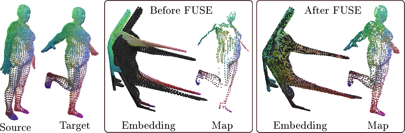
The validity of this construction rests on the nature of the FM solutions and the shared anchor distribution. While FM training relies on independent random couplings between Gaussian and data samples, this randomness affects only the conditional velocity fields, not the learned flow. Theorem 2 in [6] shows that marginalizing the conditional fields \(u_t(x \mid x_1)\) over \(x_1 \sim p_1\) recovers the unique marginal field \(u_t\) generating the probability path between \(p_1\) and \(p_0\); since this field is determined by \((p_1, p_0)\) alone, so is the induced flow \(\psi_t\). Consequently, if \(E(S_1) = E(S_2) = p_1\), the flows \(\psi^1\) and \(\psi^2\) coincide regardless of the couplings used during training, and when \(E(S_1)\) and \(E(S_2)\) are similar, their composition \(\psi^{2} \circ (\psi^{1})^{-1}\) aligns \(E(S_1)\) to \(E(S_2)\) and produces accurate correspondences (3). For this reason, points with similar embeddings from different shapes are mapped to nearby regions within the anchor (green box in 1), provided that both shapes share the same semantic structure.
The same reasoning also highlights when FUSE can be effective. When \(\mathcal{S}_1\) and \(\mathcal{S}_2\) differ by a transformation to which \(E\) is not invariant, the distributions \(E(\mathcal{S}_1)\) and \(E(\mathcal{S}_2)\) become dissimilar and not alignable by the flow composition. Instead, when the two embedding distributions share the same semantic structure, by forcing the image of \(E(\mathcal{S}_1)\) to align with \(E(\mathcal{S}_2)\) before applying KNN (3), FUSE reduces the sensitivity to embedding variations. This is why, as the isometry decreases (2) or the landmark placement becomes noisy (4), the advantage of FUSE over other methods tends to increase.

4.3 Embedding Selection↩︎
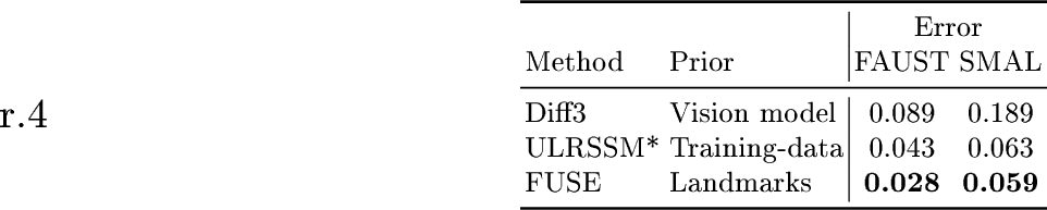
The choice of embedding \(E\) is critical. First, the generalization of FUSE to any 3D representation depends on \(E\) being computable and invariant over 3D representations. Secondly, the embedding determines the properties of the FUSE map (e.g., shape matching needs some \(E\) that captures metric and semantic information about the shapes). Every shape matching pipeline relies on assumptions that inject prior knowledge into the process. These assumptions are necessary to resolve fundamental ambiguities, most notably intrinsic symmetries, which cannot be disambiguated from purely geometric information alone. Past methods encode this prior in different ways: [29] learns a feature extractor in an unsupervised manner, where the (data) prior is induced by training over a collection of shapes; [50] leverages a pretrained large-scale vision model to extract semantic information from rendered views of meshes; [21] relies on informative spectral signatures. Each of these strategies introduces representation-specific dependencies that limit their applicability: spectral bases, rendering pipelines, or available training data.
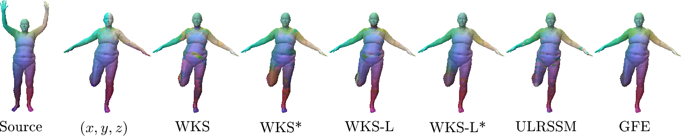
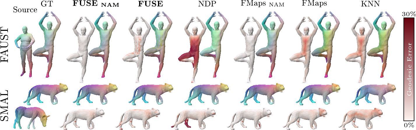
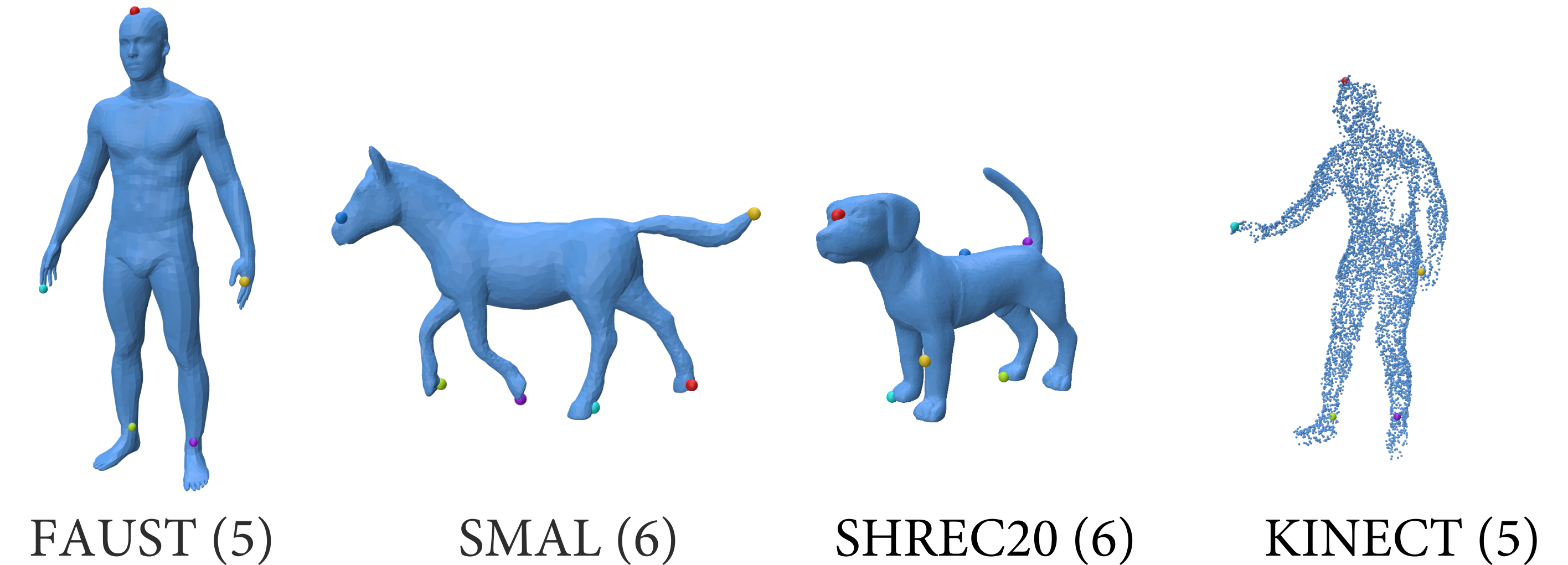
In contrast, 3D coordinates (, “identity” embeddings) are universally available but lack intrinsic geometric or semantic meaning, making them unsuitable for shape correspondence. One effective alternative is the Geodesic Feature Embedding (GFE), which represents surface points as vectors of geodesic distances to a small set of landmarks \(L\), yielding a compact embedding in \(\mathbb{R}^{|L|}_{+}\) that encodes the intrinsic geometry. Landmarks provide a minimal yet powerful form of prior: they provably resolve intrinsic symmetries by anchoring the semantic orientation of the shape, and are consistently employed in axiomatic shape matching methods derived from the Functional Maps [25] framework. In our case, landmarks are manually selected on one shape (5 or 6 depending on the semantics of the dataset) and transferred to the rest of the dataset via ground truth correspondences; 16 in the supplementary material shows the selected landmarks for each dataset. As shown in 5, despite this simple prior, FUSE with landmark-based GFE achieves the lowest correspondence error on both FAUST and SMAL against state-of-the-art prior-based methods [29], [50].
Importantly, different algorithms have been developed to compute or efficiently approximate geodesic distances on triangle meshes, signed distance fields, and point clouds, such as Dijkstra’s shortest path algorithm, the heat method [52], and fast marching [53]. While computing geodesic distances generally involves estimating the underlying surface, established methods exist (e.g. [52]) that do so implicitly with stable results. As a consequence, FUSE does not require explicit surface estimation over point clouds and can employ them directly as an input representation.
However, geodesic embeddings are not naturally aligned across shapes from a distributional perspective as a non-rigid deformation can significantly alter the geodesic distances between points. With FUSE, the flow composition acts as a probabilistic alignment mechanism: by mapping geodesic features through the Gaussian prior, we obtain distributional alignment across shapes, as shown in 3 3.
| FAUST | SMAL | |||||||||||
|---|---|---|---|---|---|---|---|---|---|---|---|---|
| 2-8 (lr)9-13 Method | \(x, y, z\) | GFE | WKS | WKS* | WKS-L | WKS-L* | ULRSSM | \(x, y, z\) | GFE | WKS | WKS-L | ULRSSM |
| Dim | 3 | 5 | 20 | 20 | 20 | 20 | 256 | 3 | 5 | 20 | 20 | 256 |
| KNN | 0.1572 | 0.0454 | 0.1007 | 0.1125 | 0.0428 | 0.0522 | 0.0723 | 0.2903 | 0.0879 | 0.2736 | 0.0697 | 0.1061 |
| 0.1488 | 0.0289 | 0.1015 | 0.0901 | 0.0556 | 0.0416 | 0.0829 | 0.3226 | 0.0595 | 0.3039 | 0.0668 | 0.1117 | |
| Dirichlet | 0.0002 | 0.0001 | 0.0056 | 0.0008 | 0.0022 | 0.0004 | 0.1847 | 0.0001 | 0.0001 | 0.0257 | 0.0131 | 0.637 |
4.3.0.1 Generality and robustness.
While GFE is our primary choice, FUSE can be applied to any pointwise embedding. To understand when it is effective, we vary both the embedding type (1) and the landmark configuration (4). In our experiments, FUSE does not appear to suffer from the increasing dimensionality: adding landmarks from 3 to 30 yields progressively better results that consistently outperform KNN (4, right); we observe the same behaviour when perturbing landmark positions by a random fraction of the shape diameter (4, left). Instead, 1 reveals that a critical factor is smoothness: GFE has very low Dirichlet energy and benefit greatly from the flow mapping, while WKS [21] and learned embeddings [29] have substantially higher Dirichlet energy, resulting in poor performance. We refer to this as curse of frequency: high-frequency embeddings induce complex distributions that are harder for the flow to align, a challenge mirroring known difficulties in Functional Maps optimization [25], [26]. GFE exhibits lower spectral complexity, making them particularly well-suited for FUSE. We note that smoothing the embeddings via projection on a small set of Laplace-Beltrami eigenbasis [54]–[56], (WKS* and WKS-L* in 1) consistently improves FUSE’s accuracy over raw features, even in non-landmark-based scenarios. This suggests that integrating smoothly learned features with flow-based models is a viable direction and fosters future work.
We note that the invertibility of the flows does not by itself induce a bijection between the shapes: the final KNN step ([eq:knn]) assigns each source point its nearest target independently, so the matching is not strictly bijective, as is standard in point-based correspondence. Since both the GFE and the flow are defined continuously over the surface, the construction naturally extends toward a continuous, fully bijective map, which we leave to future work.
4.4 Flow matching over Diffusion↩︎
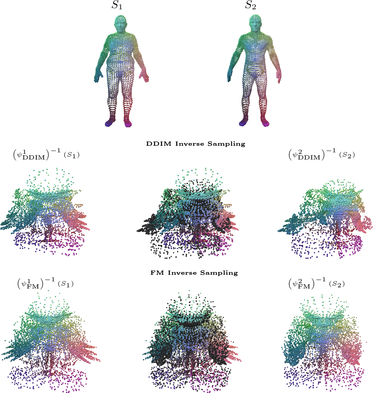
Building on the recent work of [18], which represents 3D shapes as probability distributions generated via a Denoising Diffusion Implicit Model (DDIM) [19], we adopt the same probabilistic representation while constructing maps between shapes using flow matching rather than DDIM. Although FM and DDIM can be similar, the former offers distinct advantages for our purposes. FM establishes an explicit relationship between the Gaussian distribution and the data distribution. This ensures that the inverse flow maps any shape back to the exact Gaussian distribution in a deterministic manner. This property guarantees that all shapes lie in an ideally shared latent space. In contrast, methods such as DDIM only asymptotically approach the Gaussian through large noise schedules, resulting in deviations from the anchor space.
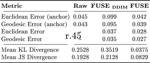
We quantify this effect in 7, evaluating shape pairs with GFE using two criteria: (1) the accuracy of nearest-neighbor correspondences both in the anchor space and in the embedding space, and (2) the JS and KL divergence between embedding distributions. We compute these metrics before and after inverting the flows using DDIM (FUSE DDIM) and FM (FUSE). The results show that FUSE achieves substantially lower divergence and higher correspondence accuracy, confirming that accurate anchoring to the Gaussian directly correlates with improved matching performance. DDIM’s inversion leads to larger deviations from the anchor and thus inferior map quality. In the supplementary materials, we provide a mathematical derivation of this crucial difference, along with additional examples.
5 Results↩︎
We evaluate our representation, considering shape matching as the main task, but also presenting possible extensions of FUSE targeting other applications.
5.1 Non-Rigid Shape Matching↩︎
We first analyze the performance of FUSE against more standardized benchmarks, considering pairs of meshes and point clouds. We then explore novel and more challenging scenarios by matching SDFs and inter-representation pairs. We restrict our analysis to landmarks-based methods, as discussed in 4.3.
5.1.0.1 Baselines.
We evaluate FUSE against baselines from different paradigms. Methods using our same geodesic feature encoding include nearest neighbor search in the embedding space (KNN) and in the anchor distribution space (FUSE ANCHOR), OT (Optimal Transport with Sinkhorn relaxation [34]), Functional Maps (FMaps) with geodesic descriptors [25], and refined variants FMaps ZO (ZoomOut[26]) and FMaps NAM (Neural Adjoint Maps [43]). Further, we also consider the original Functional Maps formulation with WKS [21], the neural extrinsic Neural Deformation Pyramid (NDP) approach [37], the vision-foundation Diff3F [50], and the data-driven ULRSSM [29]. Finally, we use FUSE to initialize ZoomOut and NAM (FUSE ZO and FUSE NAM).
5.1.0.2 Datasets.
We evaluate our method on well-established datasets for non-rigid shape matching: FAUST [57] (near-isometric human meshes), SMAL [29], [58] (non-isometric quadruped meshes), SHREC20 [59] (strongly non-isometric animal meshes), and KINECT [43], [60] (human point clouds). We manually pick 5 landmarks for humans and 6 for animals, 16 in the supplementary shows the selected landmarks for each dataset.
5.1.0.3 Metrics.
We evaluate the quality of correspondence using four metrics: two measures of accuracy, Euclidean (Eucl.) and geodesic (Geod.) distances [61], as well as Dirichlet energy [62] and coverage of the computed maps. Lower values are better for the first three metrics, while a higher value is better for Coverage. Quantitative results are reported in 2, qualitative in 8, and plots with the full distribution of the metrics in 17 of the supplementary material.
| FAUST (quasi-iso) | SMAL (non-iso) | SHREC20 (strong non-iso) | Kinect (point cloud) | |||||||||||||
|---|---|---|---|---|---|---|---|---|---|---|---|---|---|---|---|---|
| 2-17 | Eucl. \(\downarrow\) | Geod. \(\downarrow\) | Dirich. \(\downarrow\) | Cov. \(\uparrow\) | Eucl. \(\downarrow\) | Geod. \(\downarrow\) | Dirich. \(\downarrow\) | Cov. \(\uparrow\) | Eucl. \(\downarrow\) | Geod. \(\downarrow\) | Dirich. \(\downarrow\) | Cov. \(\uparrow\) | Eucl. \(\downarrow\) | Geod. \(\downarrow\) | Dirich. \(\downarrow\) | Cov. \(\uparrow\) |
| KNN | 0.0454 | 0.0434 | 0.0022 | 0.2452 | 0.0879 | 0.0836 | 0.0016 | 0.1364 | 0.1083 | 0.1036 | 0.0063 | 0.1446 | 0.1119 | 0.1095 | 0.0025 | 0.0995 |
| OT [34] | 0.0926 | 0.0856 | 0.0016 | 0.0890 | 0.0779 | 0.0741 | 0.0012 | 0.1129 | 0.1252 | 0.1168 | 0.0060 | 0.1001 | 0.1327 | 0.1273 | 0.0047 | 0.0748 |
| FMap [25] | 0.0401 | 0.0400 | 0.0016 | 0.3236 | 0.0756 | 0.0744 | 0.0018 | 0.2162 | 0.1381 | 0.1411 | 0.0077 | 0.2037 | 0.0810 | 0.0779 | 0.0031 | 0.1683 |
| FMapWKS [21] | 0.0331 | 0.0334 | 0.0017 | 0.3759 | 0.0647 | 0.0623 | 0.0023 | 0.2585 | 0.1197 | 0.1131 | 0.0203 | 0.2380 | 0.0723 | 0.0718 | 0.0045 | 0.2211 |
| FMapZO [26] | 0.0207 | 0.0195 | 0.0009 | 0.6969 | 0.0625 | 0.0611 | 0.0065 | 0.4706 | 0.1454 | 0.1480 | 0.0152 | 0.3495 | 0.0706 | 0.0710 | 0.0062 | 0.4043 |
| FMapNAM [43] | 0.0245 | 0.0240 | 0.0009 | 0.6323 | 0.0617 | 0.0589 | 0.0015 | 0.4694 | 0.1041 | 0.0962 | 0.0082 | 0.2860 | 0.0689 | 0.1118 | 0.0026 | 0.3494 |
| NDP [37] | 0.0702 | 0.0886 | 0.0020 | 0.4893 | 0.0555 | 0.0675 | 0.0010 | 0.4818 | 0.0698 | 0.0649 | 0.0013 | 0.5016 | 0.0457 | 0.0438 | 0.0012 | 0.4190 |
| Diff3f [50] | 0.0697 | 0.1109 | 0.0497 | 0.3075 | 0.1594 | 0.2278 | 0.0560 | 0.2146 | 0.0876 | 0.1036 | 0.0443 | 0.1579 | 0.1394 | 0.1732 | 0.0755 | 0.1448 |
| Diff3f FMap [50] | 0.0553 | 0.0886 | 0.0036 | 0.4427 | 0.1283 | 0.1943 | 0.0114 | 0.2789 | 0.1173 | 0.1357 | 0.0133 | 0.2376 | 0.1880 | 0.2087 | 0.0362 | 0.0565 |
| ULRSSM [29] | 0.0092 | 0.0109 | 0.0011 | 0.7302 | 0.0370 | 0.0374 | 0.0030 | 0.4936 | 0.3286 | 0.3496 | 0.2299 | 0.1337 | N/A | N/A | N/A | N/A |
| FUSEANCHOR | 0.0425 | 0.0390 | 0.0241 | 0.3483 | 0.0579 | 0.0542 | 0.0185 | 0.3708 | 0.0912 | 0.0806 | 0.0538 | 0.3619 | 0.0983 | 0.0925 | 0.0328 | 0.2459 |
| DDIM | 0.0402 | 0.0407 | 0.0023 | 0.2973 | 0.0921 | 0.0879 | 0.0016 | 0.1500 | 0.0856 | 0.0797 | 0.0030 | 0.2214 | 0.1106 | 0.1101 | 0.0025 | 0.1326 |
| 0.0289 | 0.0274 | 0.0066 | 0.5320 | 0.0595 | 0.0576 | 0.0075 | 0.5156 | 0.0975 | 0.0896 | 0.0339 | 0.5278 | 0.0969 | 0.0914 | 0.0137 | 0.4931 | |
| ZO | 0.0200 | 0.0189 | 0.0009 | 0.7127 | 0.0437 | 0.0413 | 0.0023 | 0.5361 | 0.1275 | 0.1312 | 0.0093 | 0.3763 | 0.0690 | 0.0662 | 0.0046 | 0.4173 |
| NAM | 0.0179 | 0.0168 | 0.0009 | 0.7027 | 0.0422 | 0.0388 | 0.0010 | 0.5520 | 0.0658 | 0.0603 | 0.0027 | 0.5342 | 0.0770 | 0.0702 | 0.0023 | 0.3904 |
5.1.0.4 Mesh correspondences.
While FMaps-based methods tend to produce smoother maps with smaller Dirichlet energy, our method standouts in terms of both Euclidean and geodesics accuracy. Due to the nature of the flows, invertible by design, FUSE achieves better coverage of the target surface overall. The introduction of refinement strategies (, ZO and NAM) adds pairwise optimization, further improves the base results of the FUSE pipeline and while considerably increasing the smoothness of the maps. Notably, initializing these refinements methods with FUSE yields better results than using the standard FMaps initialization, particularly evident in the case SHREC20 with strongly non-isometric pairs. Geodesic distances are particularly sensitive to deviations from isometry, and even though corresponding points can be associated with structurally similar distance distributions, actual values may wildly vary. We also observe that, in the more challenging scenario of non-isometric pairs, FUSE ANCHOR achieves marginally better accuracy than our approach, at the cost of a considerably higher Dirichlet energy and lower coverage. This suggests that the lack of smoothness in the maps produced by FUSE depends on the flow inversion from the surface to the anchor distribution, which is a non-smooth operation. ULRSSM [29] achieves the best results on FAUST and SMAL, but under performs substantially on SHREC20. As a data-driven method, it requires extensive training on a large dataset, it is restricted to meshes, whereas our flows can be efficiently trained from different representations and easily composed.
5.1.0.5 Point cloud correspondences.
Point cloud matching presents a unique challenge: FUSE requires reliable geodesic distances and sufficient surface coverage, both of which are difficult to guarantee on unstructured data, since the surface information outside of the vertices is unknown. This degrades FUSE’s performance relative to extrinsic methods like NDP [37], which bypasses geodesics entirely at the cost of failing under strong non-rigid deformations (e.g., FAUST). However, FUSE still outperforms non-refined geodesic methods (KNN, OT, FMaps), proving that the flow mechanism itself adds value.
5.2 Alternative Representations↩︎
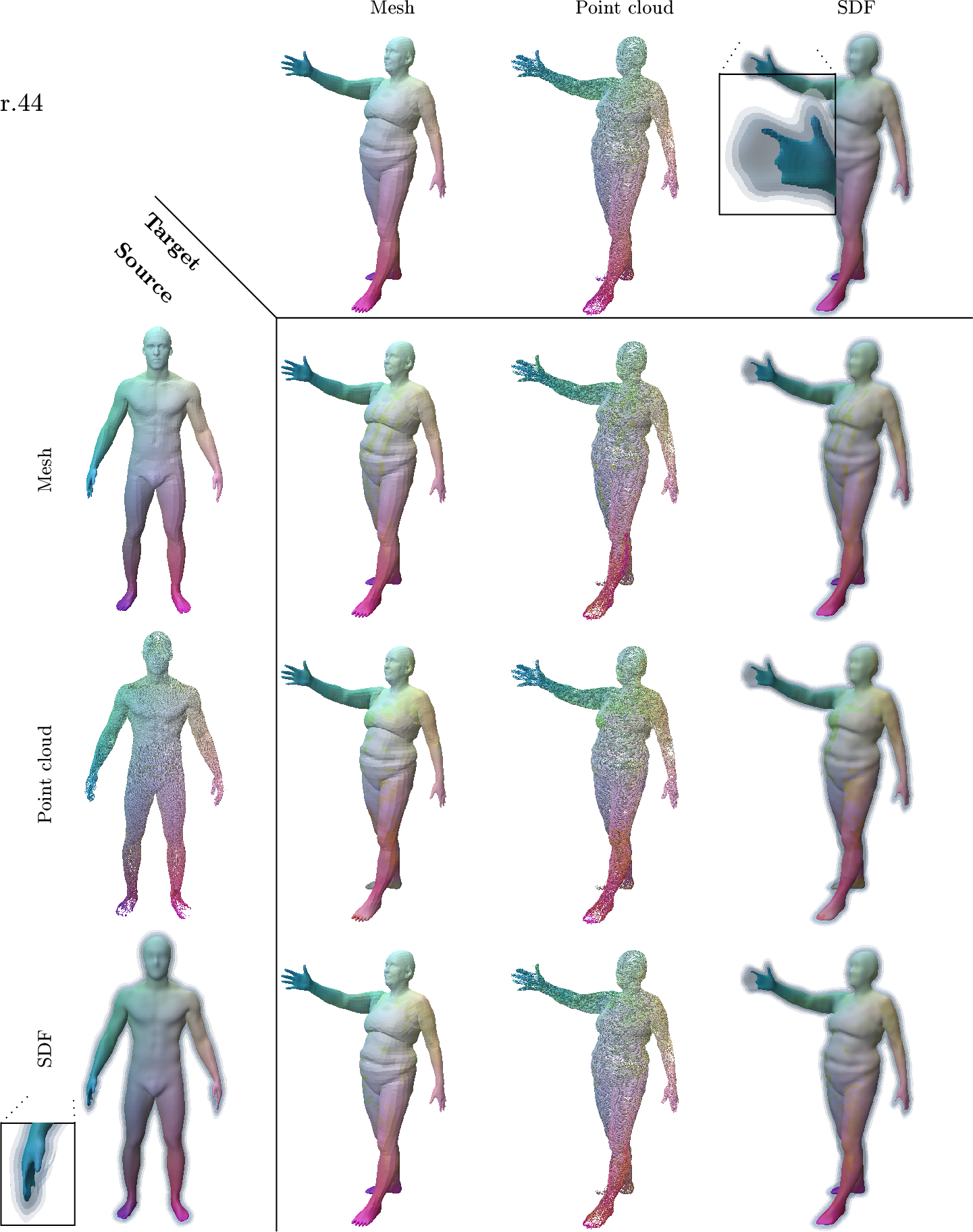
Since FUSE only requires the ability to sample points from a surface and to compute single-to-all geodesic distances, it enables shape matching in a broader class of representations, such as Signed Distance Functions (SDFs), as well as inter-representation matching (see 9).
5.2.0.1 Inter-representation matching.
We conduct experiments on shape pairs from different FAUST-like collections: from the original FAUST meshes, we extract the vertices to use as point clouds, and we compute SDFs as discussed in the previous paragraph. For each shape, geodesics are computed sticking to the constraints of the representation (, heat geodesics [52] on point clouds, Dijkstra on mesh or voxel grid). As mentioned in 5.1, FUSE inevitably struggles on matching tasks involving only point clouds, but achieves results comparable to mesh-to-mesh matching when at least one shape is represented as mesh or SDF. We provide an example of matching for all possible combinations of meshes, point clouds and SDFs in 9. A deeper analysis is presented in the supplementary material.
5.2.0.2 SDFs shape matching.
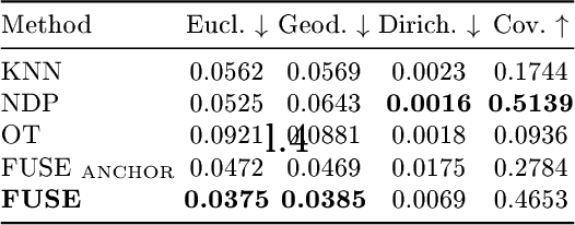
To our knowledge, no dataset exists to evaluate quantitatively matching between SDFs, so we introduce a new benchmark derived from FAUST. For each shape, we train a neural implicit model following [8], and for evaluation, we project the original mesh vertices onto the corresponding SDF surface, ensuring accuracy is always measured on the original mesh geometry. We note that this implicit reconstruction may alter the topology of some shapes. To apply FUSE, we uniformly sample \(\sim\!10^5\) points from the zero level set and voxelize each SDF surface to compute geodesic distances via Dijkstra. As in 5.1, these geodesic embeddings are then used to train the flow models. 10 reports the results for all shapes whose SDFs preserve valid topology.
FUSE provides a matching estimation without pair-specific supervision, additional training, or fine-tuning and with results comparable or better than other methods. While ZO and NAM refinement methods can be applied between meshes and point clouds to greatly improve the matching quality, these methods cannot be used on SDFs where FUSE added value is most significant, as it provides the most accurate maps compared to other baselines.
5.3 Applications↩︎
FUSE allows to model 3D surfaces as probability distributions via surface sampling and to compute maps without explicit optimization, effectively making it a “bridge” between distinct representations. We exploit this peculiar property to use FUSE as a backbone for various tasks other than pure shape matching.
5.3.0.1 Human scans fitting and skinning.
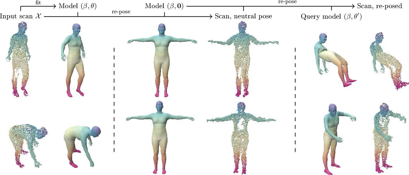
Given the scan of a human body, represented as a 3D point cloud \(\mathcal{S}\), we use FUSE to match it to a triangle mesh representing the neutral pose \(\mathcal{T}\) of a templated body model, obtained with SMPL-X [63]. By exploiting the correspondence, we can easily fit the body model’s parameters to approximate \(\mathcal{S}\) via minimization of the MSE between corresponding points. This procedure, whose results we show in the left column of 11, yields style and pose vectors \((\beta,\theta)\). If we compute the vertex offsets from the the SMPL-X output for the optimized \(\theta\) to the neutral pose \(\mathcal{T}\), we can apply them “as-is” to the corresponding points in \(\mathcal{S}\) to obtain the point cloud in neutral pose. Finally, given a novel pose vector \(\theta'\), we can iterate this process to obtain the scan in the required pose. Two example applications of our pipeline are depicted in 11.
5.3.0.2 Mesh parametrization.
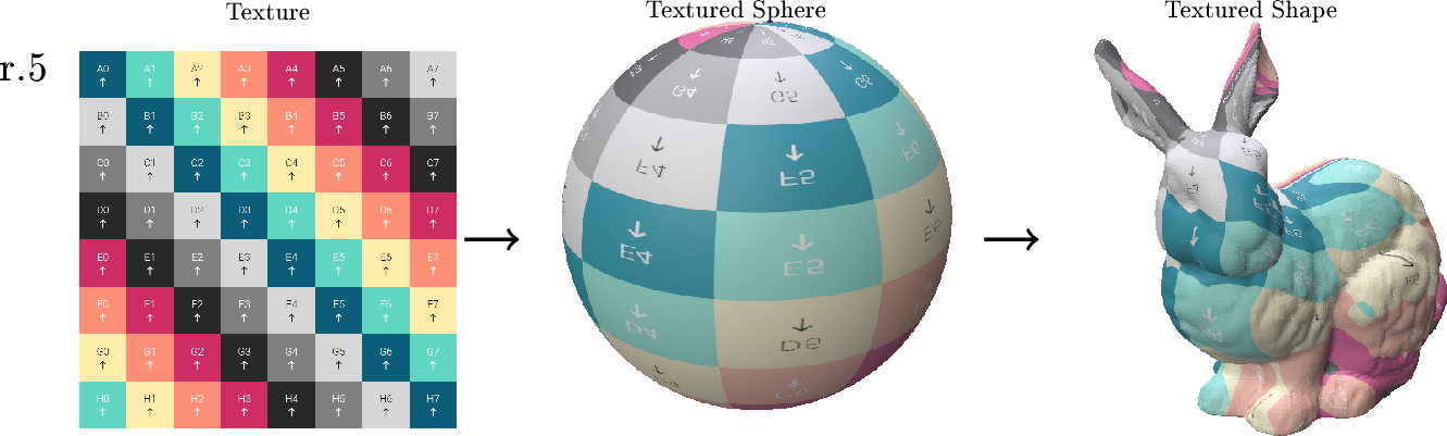
Given a genus-zero surface \(\mathcal{S}\) and a reference sphere \(\Phi\), we train flows from a Gaussian to each shape using 3D coordinates as embeddings. Composing these flows yields a bijection between \(\mathcal{S}\) and \(\Phi\), allowing us to transfer the sphere’s UV parametrization to the shape. As FUSE maps may lack smoothness (see 5.1), transferred UVs are used to supervise an MLP that predicts continuous UV coordinates, enforcing a smooth prior. Since the MLP operates in the embedding space, the procedure applies to any representation supported by FUSE. In this setting, 3D coordinates are sufficient, as no semantic consistency is required. In 12 we show an example.
5.3.0.3 Volume matching.
Our representation-agnostic formulation naturally extends to volumetric shapes, three-dimensional manifolds with well-defined geodesic distances, enabling targeting of volume-matching tasks. We apply FUSE to tetrahedral meshes, comparing it to Volumetric FMaps [64]. Results from 14 and 13 mirror our analysis on the surface scenario: comparable or improved accuracy, particularly in case of strong non-isometry, where the functional approach struggles. Details on the metrics are in the supplementary materials.

Figure 14: 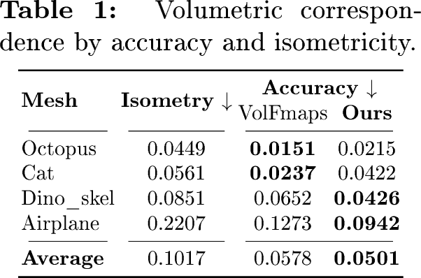 .
.
6 Conclusions and Limitations↩︎
We presented FUSE, a representation for maps between shapes based on Flow Matching. By composing per-shape invertible flows through a shared anchor distribution, FUSE produces accurate, high-coverage correspondences that are agnostic to the underlying geometric representation, supporting meshes, point clouds, SDFs, and volumetric data. Its probabilistic formulation offers an alternative to classical correspondence-based pipelines and provides a concrete starting point for works integrating learned features with flow-based alignment.
FUSE has three main limitations. First, symmetry disambiguation depends entirely on the embedding: geodesic landmarks handle this well, but embeddings lacking symmetry-breaking information (e.g., WKS) lead to degraded results. Second, the reliance on consistent geodesic distances limits its effectiveness on point clouds and makes it unsuitable for partial matching in its current form. Third, the final KNN retrieval step ([eq:knn]) makes the matching not strictly bijective, as is standard in point-based methods, though the continuity of both the GFE and the flow already supports a continuous solution. Extending FUSE to partial settings [65], [66], enforcing full bijectivity, and integrating learned smooth features are natural directions for future work.
Acknowledgements↩︎
Lorenzo Olearo’s PhD is funded by MUR under the grant “Dipartimenti di Eccellenza 2023-2027” of the Department of Informatics, Systems and Communication of the University of Milano-Bicocca, Italy. Daniele Baieri’s research is supported by a Humboldt PostDoc Fellowship from the Alexander von Humboldt Foundation and previously by the PRIN project GEOPRIDE, 2022-NAZ-0115, CUP H53D23003400001. This work was supported by the NVIDIA Corporation with the RTX A5000 GPUs granted through the Academic Hardware Grant Program to the University of Milano-Bicocca for the project “Learned representations for implicit binary operations on real-world 2D-3D data.”
7 Additional FUSE Details↩︎
7.1 Implementation Details↩︎
To implement the flows, we use the open-source flow_matching library [51] and parametrize the vector field using a simple
neural architecture. Specifically, we employ a 256-dimensional, 6-layer MLP with Swish activations [67], conditioned on both the input features \(x \in
\mathbb{R}^d\) and a scalar time variable \(t\). Before input to the MLP, the features \(x\) and \(t\) are concatenated and processed through a
Fourier feature encoder with six frequencies, resulting in \((d+1)\,(6 \times 2) +
(d+1)\) features. A final linear layer projects the hidden representation back to the original input dimension \(d\). Optimization is carried out similarly as in [18]. We trained on a single NVIDIA A5000 GPU for \(10^4\) epochs, sampling \(5 \cdot 10^4\)
points per epoch uniformly from the surface of each input shape. This setup requires less than 2 GB of GPU memory and takes approximately 2 minutes per shape. Our implementation will be made publicly available upon publication.
Comparing our setup to the one proposed in [18], our choices drastically reduce computation time for training a single flow. While some design decisions in GeomDist can be advantageous for learning high-quality representations of highly detailed input shapes, our approach optimizes representations that are sufficiently accurate for our needs within minutes instead of the several hours reported in the original GeomDist implementation.
7.2 Further Details on the Comparison Between FM and DDIM↩︎
In this section, we show additional details highlighting the differences between our method, built upon the FM framework, and the equivalent implementation with DDIM, which is the basis of GeomDist [18].
@clcccc|cccc|cccc@ & & & &
(l)3-14 & & Eucl. \(\downarrow\) & Geod. \(\downarrow\) & Dirich. \(\downarrow\) & Cov. \(\uparrow\) & Eucl. \(\downarrow\) & Geod. \(\downarrow\) & Dirich. \(\downarrow\) & Cov. \(\uparrow\) & Eucl. \(\downarrow\) & Geod. \(\downarrow\) & Dirich. \(\downarrow\) & Cov. \(\uparrow\)
& KNN & 0.0454 & 0.0434 & 0.0022 & 0.2452 & 0.1480 & 0.1404 & 0.0016 & 0.0254 & 0.0543 & 0.0549 & 0.0022 & 0.1842
& OT [34] & 0.0926 & 0.0856 & 0.0016 &
0.0890 & 0.0747 & 0.0722 & 0.0028 & 0.0472 & 0.0965 & 0.0910 & 0.0017 & 0.0945
& NDP [37] & 0.0702 & 0.0886 & 0.0020 & 0.4893 & 0.0535 & 0.0643
& 0.0016 & 0.4828 & 0.0572 & 0.0712 & 0.0017 & 0.5114
& knn-in-gauss & 0.0425 & 0.0390 & 0.0241 & 0.3483 & 0.1121 & 0.1047 & 0.0395 & 0.2262 & 0.0505 & 0.0494 & 0.0247 & 0.3107
& Ours & 0.0289 & 0.0274 & 0.0066 & 0.5320 & 0.0957 & 0.0890 & 0.0184 & 0.3761 & 0.0373 & 0.0375 &
0.0081 & 0.4816
& KNN & 0.1580 & 0.1508 & 0.0162 & 0.0129 & 0.0695 & 0.0685 & 0.0034 & 0.1540 & 0.1533 & 0.1465 & 0.0153 & 0.0117
& OT [34] & 0.1662 & 0.1556 & 0.0145 & 0.0339 &
0.0836 & 0.0802 & 0.0025 & 0.1156 & 0.1629 & 0.1533 & 0.0142 & 0.0378
& NDP [37] & 0.0547 & 0.0650 & 0.0017 & 0.4813 &
0.0530 & 0.0638 & 0.0018 & 0.4648 & 0.0578 & 0.0715 & 0.0018 & 0.4753
& knn-in-gauss & 0.0805 & 0.0757 & 0.0300 & 0.1823 & 0.0650 & 0.0639 & 0.0197 & 0.2333 & 0.0645 & 0.0643 & 0.0123 & 0.3995
& Ours & 0.0695 & 0.0680 & 0.0129 & 0.3725 & 0.0645 & 0.0643 & 0.0123 & 0.3995 & 0.0730 & 0.0716 & 0.0107 & 0.3045
& KNN & 0.0554 & 0.0554 & 0.0020 & 0.1697 & 0.1451 & 0.1387 & 0.0016 & 0.0254 & 0.0562 & 0.0569 & 0.0023 & 0.1744
& OT [34] & 0.0916 & 0.0873 & 0.0019 & 0.0851
& 0.0751 & 0.0735 & 0.0033 & 0.0489 & 0.0921 & 0.0881 & 0.0018 & 0.0936
& NDP [37] & 0.0530 & 0.0627 & 0.0015 & 0.5085 & 0.0535 &
0.0630 & 0.0016 & 0.4691 & 0.0525 & 0.0643 & 0.0016 & 0.5139
& knn-in-gauss & 0.0475 & 0.0465 & 0.0194 & 0.2706 & 0.1051 & 0.0979 & 0.0204 & 0.1612 & 0.0472 & 0.0469 & 0.0175 & 0.2784
& Ours & 0.0358 & 0.0361 & 0.0061 & 0.4775 & 0.1004 & 0.0932 & 0.0102 & 0.2680 & 0.0375 & 0.0385 & 0.0069
& 0.4653
| Method | Ours | Ours-ZO | Ours-NAM | fmap-wks | fmap | fmap-ZO | fmap-NZO | knn-in-gauss | ndp | ot | knn | ||||||||||||||||||||||
|---|---|---|---|---|---|---|---|---|---|---|---|---|---|---|---|---|---|---|---|---|---|---|---|---|---|---|---|---|---|---|---|---|---|
| time (s) \(\downarrow\) | 2.50 | 4.27 | 26.59 | 25.80 | 0.57 | 7.95 | 39.26 | 2.37 | 3.36 | 1.47 | 0.05 | ||||||||||||||||||||||
| euclidean error \(\downarrow\) | 0.0266 | 0.0093 | 0.0096 | 0.0270 | 0.0436 | 0.0097 | 0.0143 | 0.0393 | 0.0616 | 0.0862 | 0.0608 |
GeomDist (GD) is based on a Denoising Diffusion Implicit Model (DDIM) framework. In this setting, the noisy data \(X_t\) evolves according to the discretized update: \[X_t = X_0 + t \epsilon,\] where \(X_0\) is the clean shape, \(\epsilon \sim \mathcal{N}(0,I)\) is Gaussian noise. We note that the Gaussian noise only dominates the data distribution asymptotically, as \(t\) grows large. This implies that the latent isotropic Gaussian distribution is reached only for \(t \to \infty\), as opposed to the finite-time interpolation guaranteed by Flow Matching. Thus, GD’s inversion map asymptotically approximates the Gaussian prior, leading to deviations from the anchor distribution and hindering anchor space similarities between different shapes. This difference underpins the improved accuracy and tighter distributional alignment we observe in our flow-matching-based method. Indeed, FUSE’s interpolation can be written as \[X_t = (1-t)X_0 + t X_1,\] where \(X_1\) is the clean shape and \(X_0 \sim \mathcal{N}(0,I)\) is Gaussian noise. We note that in this case, we have a clear notion of the time at which we sample one of the two distributions, maintaining consistency between different flows. In 15, we show a qualitative comparison between two three-dimensional flows. Inverting the source and target flows to their Gaussian-like base distributions reveals a subtle discrepancy in the DDIM case. Under a Flow-Matching noise schedule, however, this discrepancy largely disappears. For visualization purposes, the inverted target is shown in black while the inverted source remains colored.
8 Evaluation↩︎
8.0.0.1 Datasets.
We evaluate our method on well-established datasets for non-rigid shape matching:
FAUST (meshes): a dataset of near-isometric human subjects in different poses [57] in a 1:1 correspondence.
SMAL (meshes): composed of different classes of quadrupeds in varying poses with strongly non-isometric deformations [58]; we use the remeshed version of the dataset [29], where shapes have different discretizations.
SHREC20 (meshes): 14 animal shapes including highly non-isometric pairs and shapes with missing parts [59]. No dense registration is provided, each pair is annotated with sparse set of landmarks; we consider all the pairs of the \(5\) test set and evaluate on the common landmarks between each shape pair.
KINECT (point clouds): Kinect acquisitions of 15 human shapes interacting with objects from the BEHAVE dataset [60] with SMPL registrations, introduced in [43].
Landmarks are placed manually at shape protrusions: 5 for humans and 6 for animals. For SHREC20 specifically, 6 points are selected from the pool of common points shared across all shapes, with evaluation performed on the remaining common point pairs. 16 illustrates the landmarks on a representative shape from each dataset.
8.0.0.2 Baselines.
For Functional Maps-based baselines, we used implementations from the GeomFuM library [68]. For NDP [37], we adopted the original source code. For volumetric FMaps [64], we considered the original MATLAB source code. For FMaps and FMaps-WKS, maps were computed using 20 basis functions. For the WKS variant, we leveraged 200 basis functions to compute descriptors, using both landmark-based and global descriptors as standard. ZoomOut and NAM [43] were implemented by performing spectral upsampling from 20 to 120 basis functions with steps of 5 basis functions. Optimal Transport (OT) computations were performed using the Sinkhorn relaxation method [34] available via the PythonOptimalTransport library [69].
8.1 Evaluation Metrics↩︎
In this Section, we provide details on how we computed all evaluation metrics employed throughout the paper. The Euclidean error is computed as: \[E_{\text{eucl}} = \frac{1}{|S_1|} \sum_{x \in S_1} \frac{\|T_{12}(x) - T_{\text{gt}}(x)\|_2}{D_{\text{eucl}}}\;\] where \(D_{\text{eucl}} = \max_{u,v\in S_2} \lVert u-v\rVert_2\). Similarly, the geodesic error is defined as: \[E_{\text{geod}} = \frac{1}{|S_1|} \sum_{x \in S_1} \frac{d(T_{12}(x), T_{\text{gt}}(x))}{D}\] where \(d\) is the geodesic distance function on \(S_2\), \(T_{12}\) is the estimated correspondence map, \(T_{\text{gt}}\) is the ground truth map, and \(D = \max_{u,v\in S_1} d(u, v)\) is the shape diameter of \(S_2\).
The Dirichlet energy of the correspondence map is computed as: \[E_{\text{Dir}} = \text{trace}(T_{12}(X_1)^\top \boldsymbol{\Lambda} T_{12}(X_1) )\] where \(\boldsymbol{\Lambda}\) and \(X_1\) are respectively the Laplacian matrix and the vertex coordinates matrix associated with the source shape \(S_1\).
Coverage measures the fraction of the target shape covered by the mapping, Importantly, we normalize the this measure by the cardinality ratio \(|S_2|/|S_1|\) to ensure comparability across shapes with varying numbers of vertices: \[\text{Cov} = \frac{|\{ y \in S_2: \exists x \in S_1, T_{12}(x) = y \}|}{|S_2|} \cdot \frac{|S_2|}{|S_1|}\]
The isometry metric evaluates the relative difference between pairwise geodesic distances on tetrahedra that are in ground truth correspondence as: \[E_{\text{iso}} = \sum_{x,y} \frac{| d_1(x,y) - d_2(T_{\text{gt}}(x), T_{\text{gt}}(y)) |}{d_1(x,y)}\] where \(d_1\) and \(d_2\) are geodesic distances on the source and target shapes respectively.
8.2 Evaluation Metrics Distribution↩︎
For a better visualization of the numerical results reported in 2 of the main paper, we provide in 17 the distribution of per-pair Euclidean error, Geodesic error, Dirichlet energy, and Coverage for each method across all four benchmarks.
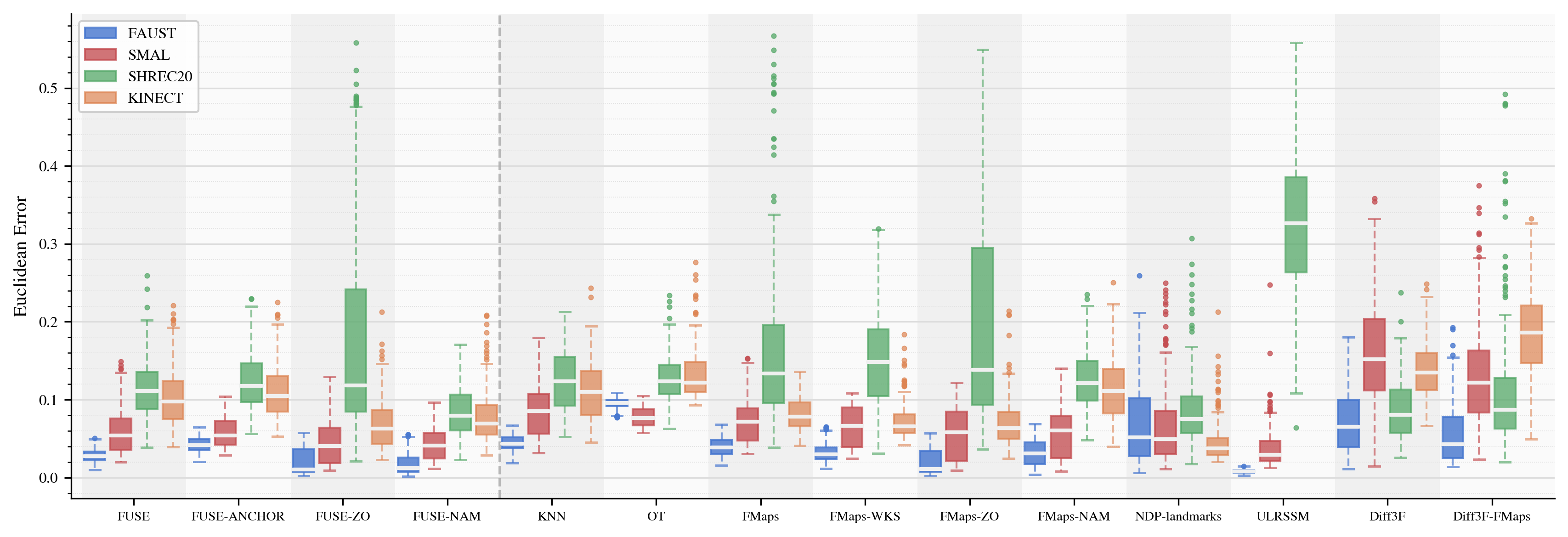
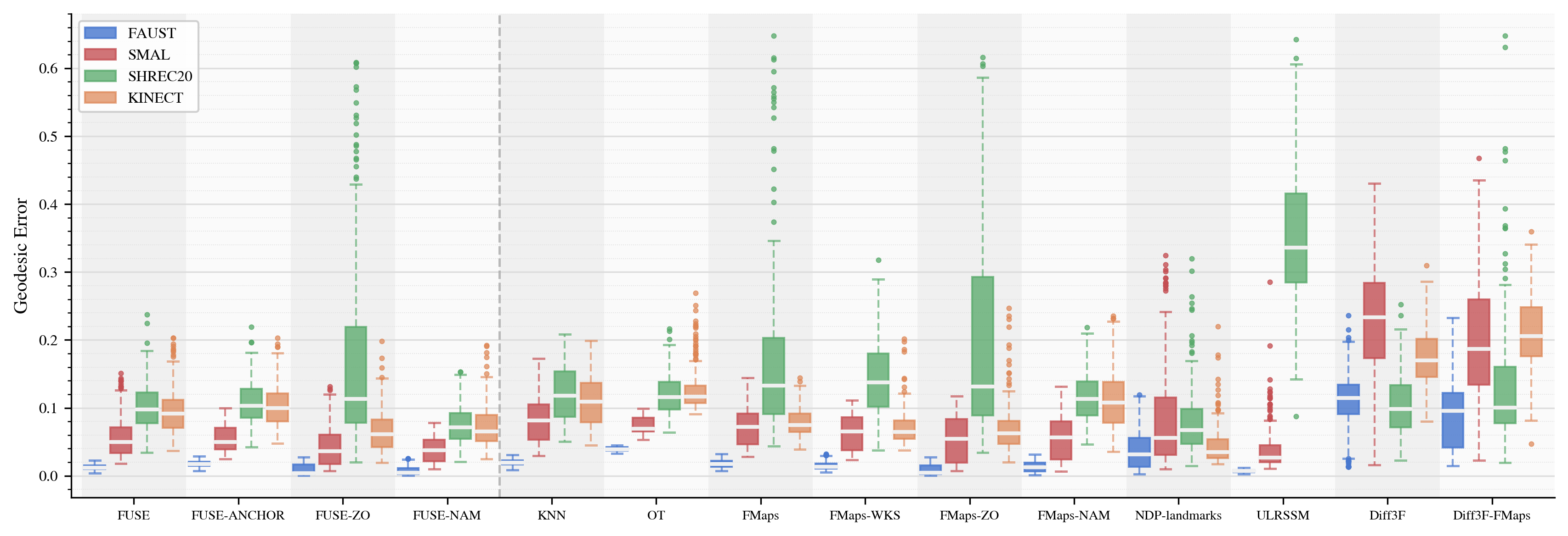
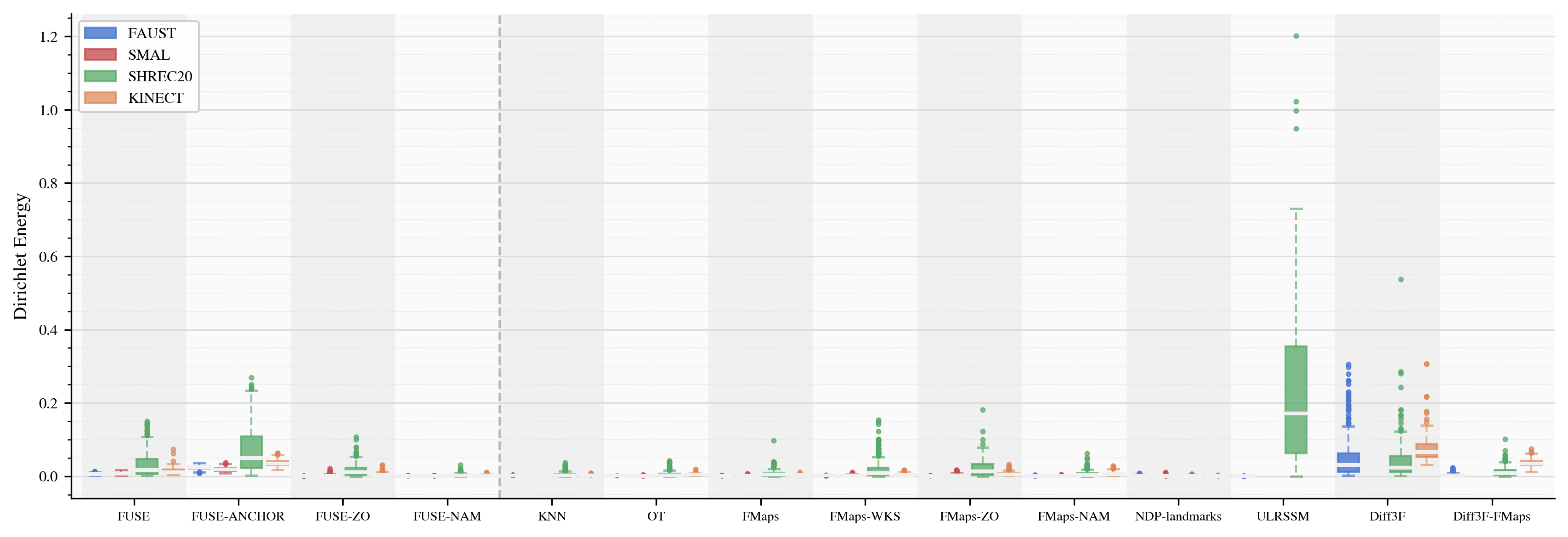
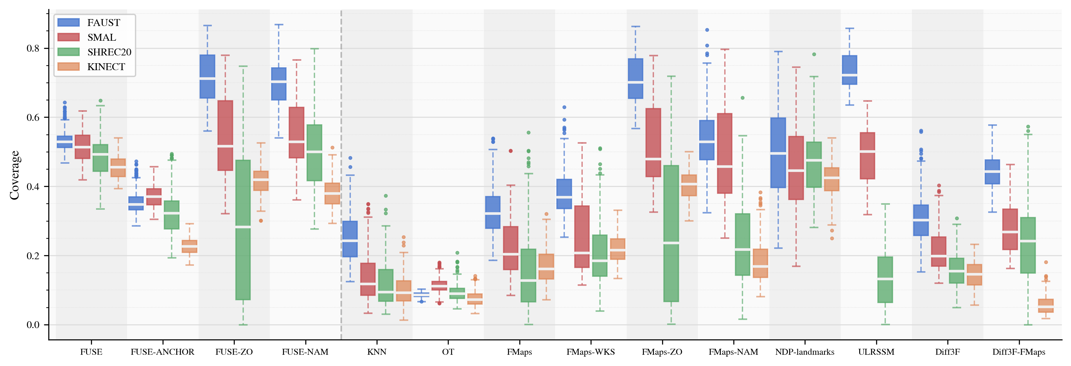
Figure 17: Distribution of Euclidean and Geodesic error, Dirichlet energy, and Coverage for each method on FAUST, SMAL, SHREC20, and KINECT. Each box spans the inter quartile range; the central line is the median while individual points are outliers. Methods left of the dashed line are ours..
8.3 Inter-Representation Quantitative Results↩︎
We follow the setting described in 5.2 to evaluate our method in the context of inter-representation matching. Out of all the baselines considered in 5.1, we only take into account those suitable for inter-representation matching, namely KNN, Optimal Transport (OT) [34] and NDP [37], together with FUSE and KNN in the Gaussian anchor space (knn-in-gauss).
¿tbl:tab:inter-rep-full? reports the full quantitative results for all the \(9\) inter-representation matching scenarios considered in 9 of the main paper. Our method stands out in terms of Euclidean and Geodesic errors when considering matching between well-defined surfaces, such as meshes and SDFs. Consistent with the pointcloud-to-pointcloud matching results on the KINECT dataset reported in 2, FUSE struggles when matching to or from point clouds, where NDP [37] instead achieves the best results across all metrics, likely due to the shared information at inference time. Furthermore, our method relies on accurate geodesic distance computations and uniform sampling of the surface, both of which are challenging to achieve on point clouds. Nonetheless, FUSE still achieves the second-best performance across most metrics in these scenarios.
9 Smoothness↩︎
In this section, we provide additional details and analysis on why smooth features are necessary for the functioning of the FUSE. Firstly, we demonstrate the effect that varying the smoothness of a feature has on the performance of FUSE by providing an example. Secondly, we demonstrate that smoothing embeddings enables FUSE to achieve better results even with high dimentional pretrained embeddings. We define the \(*\) operation as the spectral filtering operation. Given an embedding \(E\), the spectral filter of \(E*\) can be obtained as follows: \[E* = \Phi_k\Phi_k^TM E\] where \(\Phi_k\) is the \(k\) truncated basis matrix obtained by the decomposition of the Laplace-Beltrami Operator of the input shape [56]. This operation is the same as that used in the main paper in Table 1, with \(k=10\).
9.0.0.1 Controlled experiment on smoothness.
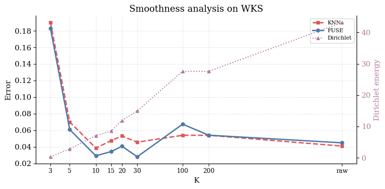
To visualize the effect of smoothness on the effectiveness of FUSE, we consider a pair of shapes from the FAUST dataset and compute their Wave Kernel Signature embeddings. We then perform spectral filtering while varying the number of eigenfunctions used. Increasing the number of eigenfunctions decreases the smoothness of the embedding and increases its Dirichlet energy.
Using these embeddings, we compute correspondences via KNN and FUSE, which highlights a distinctive behavior of our method. In Figure 18, we visualize this experiment. We observe that FUSE improves the results when the embeddings are smooth, whereas for high-frequency embeddings, it degrades performance with respect to KNN. Interestingly, the combination of smoothing and FUSE yields the overall best results.
9.0.0.2 Smoothed pretrained embeddings.
| Original | * | |
|---|---|---|
| KNN | 0.072 | 0.074 |
| 0.082 | 0.068 | |
| Dirichlet | 0.1847 | 0.0016 |
r0.38
We then consider pretrained embeddings obtained with the method of [29]. We show that applying the smoothing operation with \(k=10\) improves the overall performance.
In Table 4, we can clearly see that smoothing combined with FUSE yields better results than the raw pretrained embeddings. This observation motivates future work on integrating FUSE directly into the pretraining phase of embedding learning, and it is consistent with previously documented benefits of smoothness in learned representations [70].
9.1 Computational Cost Analysis↩︎
In Flow Matching, the vector field is parameterized using a neural network. Consequently, beyond the computational cost of evaluating the network itself, one must also take into account the numerical integration of the field to obtain the actual flow. The computational cost of this process depends on both the choice of solver and the number of integration steps employed. In 6, we present a comparison between Euler and Midpoint solvers with varying numbers of integration steps, applied to both the forward and inverse flow processes on the FAUST dataset. Notably, the accuracy of the resulting maps is predominantly influenced by the precision of the forward flow integration, whereas lower integration precision in the inverse flow has a less pronounced impact. As expected, the Midpoint solver with a larger number of integration steps achieves better accuracy than naive Euler integration, albeit at the expense of increased computational time. Conversely, employing fewer steps with Midpoint or using a simpler solver such as Euler accelerates inference but results in a measurable reduction in mapping accuracy.
9.2 FUSE with Different Anchors↩︎
A shape can be represented as a flow starting from any distribution from which samples can be drawn. Naturally, the choice of this starting distribution can influence the quality of the final maps obtained via the flow composition employed in FUSE. In our experiments we used a standard Gaussian distribution as the anchor, however, alternative choices are not only possible but may also be better suited for other applications beyond the scope of this work.
The fundamental requirement for the anchor distribution in FUSE is robustness with respect to flow inversion from the surface of the shape to itself. In 19, we provide a qualitative comparison of different starting distributions in \(\mathbb{R}^3\) for visualization purposes, while 5 reports corresponding quantitative results on the FAUST dataset with different multidimensional distributions. As illustrated in 19, sampling from the initial distribution \(X_0\) and subsequently applying the flow \(\psi(X_0)\) produces a shape distribution that deviates slightly from the target shape surface on which the flow was trained. By performing a backward integration of the flow, \(\psi(\psi(X_0))^{-1}\), we recover an approximation of the identity map, with discrepancies coming from the non-smoothness of the mapping from volume to surface of the inverted flow.
| Anchor distribution | Eucl. \(\downarrow\) | Geod. \(\downarrow\) | Dirich. \(\downarrow\) | Cov. \(\uparrow\) |
|---|---|---|---|---|
| Standard Gaussian | 0.0289 | 0.0274 | 0.0066 | 0.5320 |
| Unit Sphere Volume | 0.0292 | 0.0290 | 0.0094 | 0.5877 |
| Unit Volume | 0.0319 | 0.0318 | 0.0146 | 0.5840 |
| Unit Sphere Surface | 0.2654 | 0.2702 | 0.2477 | 0.3137 |
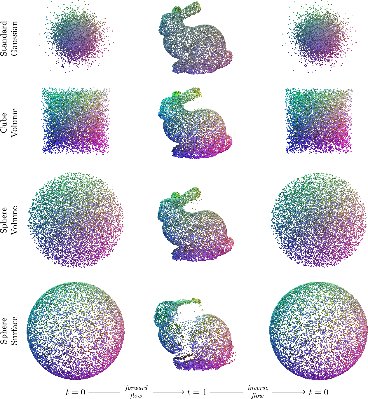
In contrast, when sampling directly from the surface of the shape and applying the inverse flow to project these points back to the anchor distribution, we observe a more pronounced deviation from the expected anchor distribution. This behavior is particularly evident in 2 and 15, where the distributions obtained via the inverted flow do not exhibit Gaussian-like characteristics. We attribute this phenomenon to the fact that the sampled points occupy only a subset of the shape’s distribution parametrized by the flow; consequently, the resulting inverted distribution corresponds to a subset of the anchor distribution.
To avoid smoothness issues during the inversion of a surface into a volume, one could consider using an initial distribution that is naturally defined on a lower-dimensional manifold, such as the surface of the unit sphere, thus having true diffeomorphic mappings between the shape and the anchor. However, as shown in 5 and 19, this choice leads to significantly worse results compared to volumetric anchors. This is likely due to the challenges associated with accurately learning flows on lower-dimensional manifolds embedded in higher-dimensional spaces, which can result in instabilities during both training and inference.
| Solver | bwd-steps | fwd-steps | Eucl. \(\downarrow\) | Geod. \(\downarrow\) | Dir. \(\downarrow\) | Cov. \(\uparrow\) | Time (s) \(\downarrow\) | ||||||||||
|---|---|---|---|---|---|---|---|---|---|---|---|---|---|---|---|---|---|
| Midpoint | 10 | 10 | 0.0419 | 0.0428 | 0.0072 | 0.2933 | 0.41 | ||||||||||
| Midpoint | 10 | 64 | 0.0344 | 0.0349 | 0.0070 | 0.4259 | 1.43 | ||||||||||
| Midpoint | 64 | 10 | 0.0438 | 0.0450 | 0.0084 | 0.3527 | 1.46 | ||||||||||
| Midpoint | 64 | 64 | 0.0289 | 0.0274 | 0.0066 | 0.5320 | 2.50 | ||||||||||
| Midpoint | 32 | 32 | 0.0337 | 0.0340 | 0.0066 | 0.4692 | 1.26 | ||||||||||
| Midpoint | 16 | 16 | 0.0368 | 0.0377 | 0.0070 | 0.3669 | 0.64 | ||||||||||
| Euler | 64 | 64 | 0.0364 | 0.0360 | 0.0075 | 0.3945 | 1.30 | ||||||||||
| Euler | 10 | 64 | 0.0756 | 0.0700 | 0.0133 | 0.2479 | 0.74 | ||||||||||
| Euler | 64 | 10 | 0.0827 | 0.0778 | 0.0065 | 0.1954 | 0.75 | ||||||||||
| Euler | 32 | 32 | 0.0514 | 0.0496 | 0.0092 | 0.2791 | 0.64 |