Bit-Accurate Modeling of GPU Matrix Multiply-Accumulate Units: Demystifying Numerical Discrepancy and Accuracy
November 14, 2025
Abstract
Modern AI accelerators rely on matrix multiply-accumulate units (MMAUs), such as NVIDIA Tensor Cores and AMD Matrix Cores, to accelerate deep neural network workloads. MMAUs expose only instruction-level or API-level interfaces of matrix multiply-accumulate (MMA) operations, while leaving internal floating-point arithmetic behaviors undocumented. Consequently, MMAUs across vendors and architectural generations often produce numerical discrepancies for identical inputs, and sometimes exhibit reduced numerical accuracy that can cause training instability. Diagnosing and understanding the root causes of these effects is challenging without white-box models of their arithmetic behaviors. This paper proposes closed-loop feature probing (CLFP), a generic and systematic framework for constructing complete arithmetic behavior models of MMA operations. Based on this framework, we analyze all MMA instructions on ten GPU architectures spanning from NVIDIA Volta to RTX Blackwell and from AMD CDNA1 to CDNA3, and derive the first bit-accurate arithmetic models for these MMAUs. Our models explain previously observed cross-platform numerical discrepancies and accuracy issues, enable white-box numerical error analysis, reveal four precision bottleneck designs and one numerical asymmetry design that significantly affect numerical accuracy, and provide software workarounds as well as design guidance for future MMAUs. This work is open-source on github.com/microsoft/MMA-Sim.
1 Introduction↩︎
Deep neural networks (DNNs) are built on massive numbers of linear algebra operations. To satisfy the rapidly growing computational demands of modern DNN workloads such as large language models (LLMs), recent AI accelerators have introduced specialized hardware units such as NVIDIA Tensor Cores [1] and AMD Matrix Cores [2] to accelerate matrix multiplications. These matrix multiply-accumulate units (MMAUs) now dominate both training and inference workloads because of their extremely high throughput, efficiency, and support for mixed-precision arithmetic. As DNN workloads scale in model size and deployment scope, the numerical behavior of MMAUs becomes increasingly critical since small discrepancies can accumulate across a large number of operations and affect reproducibility and training stability (§2).
Despite performing the same mathematical operation, MMAUs from different AI accelerators are not numerically equivalent. Even with bit-identical inputs, different MMAU implementations can produce different floating-point results. Such discrepancies are pervasive across vendors [3] and also occur across architectural generations from the same vendor [4]. These hardware-level numerical discrepancies could propagate through the software stack and manifest as inconsistencies in end-to-end DNN workloads, resulting in poor reproducibility across different AI accelerators.
Compounding the problem, the underlying arithmetic behaviors of MMAUs, i.e., the hardware-specific floating-point computation mechanism for the matrix multiply-accumulate (MMA) operations, are poorly documented and effectively a black box, leaving developers without a clear understanding of how numerical results are produced. As a result, their impacts on numerical accuracy are often discovered only after they surface in large-scale systems. Recent incidents illustrate this issue. DeepSeek developers [5], [6] reported that poor summation precision in FP8 MMA operations on NVIDIA Hopper Tensor Cores degraded training accuracy, while PyTorch developers [7] found that subnormal flushing in FP16 MMA operations on AMD CDNA2 Matrix Cores caused training instability. In both cases, the root causes stem from obscure arithmetic behavior of MMAUs.
These observations reveal a fundamental gap: the lack of a white-box understanding of MMAU arithmetic behavior. Without such a foundation, numerical analysis remains empirical and reactive, making it difficult to predict accuracy, diagnose issues, or design principled mitigations. A systematic white-box model of MMAU arithmetic behavior is therefore essential for rigorous and proactive reasoning about the numerical behavior of modern AI systems.
However, obtaining a white-box model for MMAUs is inherently difficult. MMAUs expose only high-level MMA interfaces at the API level (e.g., on cloud TPUs [8]) or the instruction level (e.g., on GPUs), while the arithmetic features that determine numerical results remain hidden inside proprietary hardware. These features include computational order, fusion granularity, internal precision, rounding behavior, and many other subtle design choices. Because the relevant feature set is neither explicitly documented nor straightforward to enumerate exhaustively, the space of possible arithmetic behaviors is effectively enormous, making exhaustive black-box exploration challenging.
In this paper, we tackle this challenge with a generic, systematic, and principled approach for constructing white-box models of MMA arithmetic behaviors from black-box testing. In particular, we propose a closed-loop feature probing (CLFP) framework (§3) that integrates arithmetic feature probing with iterative model refinement for general MMA operations. Given an MMA interface, the framework leverages carefully-designed edge-case inputs and corresponding outputs to probe key arithmetic features. Based on these observations, we build an executable arithmetic behavior model and iteratively refine it through a probe-infer-verify-revise loop until the model is verified to reproduce the MMA interface bit by bit. This closed-loop methodology enables reliable modeling of black-box MMAU arithmetic behavior in AI accelerators.
In this work, we apply CLFP to instruction-level interfaces of MMAUs. Based on the CLFP framework, we systematically analyze all instruction-level floating-point MMA operations on ten GPU architectures, spanning from NVIDIA Volta to RTX Blackwell and from AMD CDNA1 to CDNA3, and construct white-box models of their arithmetic behaviors (§4). Our models reveal, for the first time, the complete and bit-accurate arithmetic behaviors of floating-point MMA operations in AI accelerators, showing that these operations are composed of different types of elementary floating-point operations with different precisions, rounding modes, computational orders, and granularities.
These white-box bit-accurate models explain previously observed numerical discrepancies across accelerators and expose the design choices that can affect numerical accuracy. For example, the models explain how the MMAUs produce six different output values (\(0.0\), \(-0.375\), \(-0.5\), \(-0.75\), \(-0.875\), and \(-1.0\)) for the same input (§5). The white-box models also enable us to quantitatively analyze the sources of numerical errors, revealing four types of precision bottlenecks and one type of asymmetry that significantly degrade the numerical accuracy of MMAUs (§6). Based on the analysis, we provide software workarounds, mitigation methods, and design guidance for future MMAUs.
We make the following contributions in our work:
A closed-loop feature probing framework. We introduce CLFP, a general methodology for deriving bit-accurate models of MMA arithmetic behavior through feature probing and iterative verification, and apply it in this work to MMAUs.
Bit-accurate modeling of GPU MMAUs. We construct the first bit-accurate arithmetic behavior models for all instruction-level floating-point MMA operations on NVIDIA Tensor Cores and AMD Matrix Cores.
MMAU numerical discrepancy analysis. We identify the differences in arithmetic behavior underlying the MMAUs, revealing the root causes of numerical discrepancies beyond floating-point non-associativity.
MMAU numerical accuracy analysis. We quantitatively analyze the design choices that affect numerical accuracy across the MMAUs, providing mitigation methods and design guidelines.
Open-source release. We open source our implementations and results to facilitate continuous testing, numerical analysis, and design space exploration.
2 Background and Related Work↩︎
2.1 Black-Box Arithmetic Behavior of MMAUs↩︎
Matrix multiply-accumulate units (MMAUs) such as NVIDIA Tensor Cores and AMD Matrix Cores [1], [2], [9] execute matrix multiply-accumulate (MMA) operations of the form \[\label{eq:mma} D_{M\times N} = A_{M\times K} \times B_{K\times N} + C_{M\times N}.\tag{1}\] Although this mathematical definition is shared, hardware implementations of MMAUs are not numerically equivalent. The underlying arithmetic behavior of an MMAU is not standardized or well documented. Vendors may choose different computational orders, accumulation precisions, intermediate rounding modes, fusion granularities, special-value handling rules, etc., while exposing high-level instructions or APIs of MMA operations only.
Nevertheless, these hidden design choices are critical because they determine how intermediate results are produced and rounded during mixed-precision execution. Consequently, two MMAUs that nominally perform the same MMA operation may still produce different bit-level outputs [3], [4]. More importantly, when discrepancies or accuracy problems surface in software, the root causes are difficult to diagnose because the relevant arithmetic behavior is invisible at the programming-model level.
2.2 Numerical Discrepancy and Accuracy Concerns↩︎
Floating-point numerical behavior has become a critical concern in modern deep learning systems. In deep neural networks (DNNs), small arithmetic differences can accumulate and amplify across layers and iterations of computation [10]. This sensitivity is particularly pronounced in large language models (LLMs), where mixture-of-experts architectures, reinforcement learning stages, and complex serving systems magnify the impact of numerical variation, resulting in significant challenges [11].
One practical concern is numerical discrepancy across hardware platforms. Even when the same model and input data are used, migrating workloads across vendors or architectural generations can produce different floating-point results [12]–[14]. Such discrepancies complicate reproducibility of deep learning experiments and create practical challenges when porting workloads across accelerator platforms [15], [16]. From the software perspective, these differences are often attributed to changes in compiler options, random seeds, mixed-precision policies, parallel execution order, etc. However, the discrepancies persist even after the software stacks are carefully aligned, indicating that the explanation is incomplete [17]–[19]. To fully understand numerical behavior, we must also account for hardware-specific arithmetic behavior.
Another practical concern is numerical accuracy and training stability. Recent incidents show that arithmetic behavior inside AI accelerators can directly affect end-to-end DNN workloads. DeepSeek developers [5], [6] reported that poor summation precision in FP8 MMA operations on NVIDIA Hopper degraded training accuracy, requiring additional FP32 accumulation on CUDA cores. PyTorch developers [7] found that FP16 MMA operations on AMD CDNA2 flush subnormal numbers to zero, which can cause FP16 training to fail to converge because subnormal values frequently arise during backpropagation. Their workaround casts FP16 operands to BF16 to increase dynamic range at the cost of precision.
Taken together, these observations point to two key insights. First, numerical discrepancies across accelerators are real and recurrent. Second, the relationship between differences in MMAU arithmetic behavior and their impact on numerical accuracy remains poorly understood. While some hardware design choices may have negligible practical effects, others can materially influence training stability and model quality. Without a clear understanding of the underlying arithmetic behaviors, it is difficult to distinguish between these cases.
2.3 Limitations of Existing Approaches↩︎
Prior work has made important progress in modeling the arithmetic behaviors of MMA accelerators. Raihan et al. [20] proposed an intuitive model that represents Tensor Core dot-products as a perfect binary tree of multiplication and addition operations, but later experiments showed that this model does not match hardware behavior faithfully. Hickmann et al. [21] designed arithmetic feature probing experiments to infer characteristics of the Tensor Core on NVIDIA Volta architecture; Fasi et al. [4] expanded arithmetic feature probing to Tensor Cores on NVIDIA Turing and Ampere GPUs; and Li et al. [22] extended this to NVIDIA Hopper Tensor Cores and AMD Matrix Cores on CDNA1 and CDNA2. Xie et al. [23] proposed a method called FPRev to rigorously infer summation order in MMA operations.
These studies reveal valuable aspects of MMAU arithmetic behaviors, but they have several limitations. First, they focus on partial arithmetic features for a limited set of architectures, which are incomplete for constructing white-box executable models. Second, their conclusions are not validated as bit-accurate end-to-end models, and some are even contradictory. For example, Hickmann et al. [21] concluded that the values in the input \(C\) are accumulated after dot products, while Fasi et al. [4] showed that they are accumulated with the products in the same fused summation. Valpey et al. [24] also reported that some previous results are inaccurate. As a result, feature probing alone is necessarily incomplete for reliable modeling. The field still lacks a systematic approach for deriving white-box, validated, bit-accurate models of MMAU arithmetic behavior.
3 Methodology and Implementation↩︎
Given a black-box interface of a matrix multiply-accumulate (MMA) operation, we propose the closed-loop feature probing (CLFP) framework to build the arithmetic behavior model \(\Phi\) such that \[\label{eq:phi} \Phi(A,B,C) = \text{MMA-Interface}(A,B,C),\tag{2}\] for any input matrices \(A\), \(B\), and \(C\) with shapes \(M\times K\), \(K\times N\), \(M\times N\) and data types specified by the interface.
3.1 CLFP Workflow↩︎
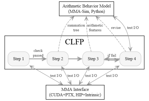
As Figure 1 shows, the workflow of CLFP consists of four testing-based steps. Through arithmetic feature testing and probing, Steps 1 and 2 deterministically decompose the MMA operation into low-level operations. Then, Step 3 probes the detailed arithmetic behavior of the low-level operation. However, the probing may be incomplete, so Step 4 leverages randomized testing to verify whether the model composed of the inferred low-level operations matches the output of the MMA interface bit by bit (Equation 2 ). If verification fails, we revise the model and repeat Steps 3 and 4.
3.1.1 Step 1: Confirming Computational Independence↩︎
To check whether the computation of \[\label{eq:dij} d_{i,j} = c_{i,j}+\sum_{k=0}^{K-1} a_{i,k}b_{k,j}\tag{3}\] depends on the indices \(i\) and \(j\), we construct the following input for the MMA interface.
We first generate \(2K+1\) random numbers: \(a_{0,0}, \dots\), \(a_{0,K-1}\), \(b_{0,0}, \dots\), \(b_{K-1,0}\), and \(c_{0,0}\). Then, we let \(a_{i,k}=a_{0,k}\), \(b_{k,j}=b_{0,j}\), and \(c_{i,j}=c_{0,0}\) for all \(0<i<M\), \(0<j<N\), and \(0\le k<K\). If the computation does not depend on the indices \(i\) and \(j\), all \(d_{i,j}\) in the output should be bitwise identical; otherwise, two elements of different indices can be different. Through extensive testing, we find that all \(d_{i,j}\) in the output matrix are bitwise identical, confirming that each output element in \(D\) is computed independently.
Therefore, we can decompose the MMA operation into \(M\times N\) independent dot-product-accumulate operations of Equation 3 and we only need to model a single one in the remaining steps. In the remainder of the paper, we simplify the notation for the dot-product-accumulate operations of any \(d_{i,j}\) into \[\label{eq:d} d = c + \sum_{k=0}^{K-1}a_{k}b_{k}.\tag{4}\]
3.1.2 Step 2: Determining Summation Order and Arity↩︎
This step decomposes the dot-product-accumulate operation (Equation 4 ) into a combination of summation operations and determines how they are combined.
In particular, Equation 4 can be transformed to \[\label{eq:sump} d=\sum_{k=0}^K p_k \text{, where } p_k=\begin{cases} a_kb_k &\text{if 0\le k < K} \\ c &\text{if k=K} \end{cases}.\tag{5}\] The summation order of Equation 5 can be represented by a summation tree with \(K+1\) leaf nodes, where a node with \(n\) child nodes represents an \(n\)-ary summation operation. Figure 2 demonstrates four typical examples. To infer the tree, we construct the following inputs for Equation 5 .
Adapting from FPRev [23], we choose a very large number \(U=2^{e_u}\) and a very small number \(v=2^{e_v}\) such that \[\label{eq:swamp} (K-1)v\pm U=\pm U\tag{6}\] in floating-point arithmetic, which means that \(\pm U\) can serve as large summands to swamp other small summands in summation. Then, for every \(0\le i < j \le K\), we construct the inputs \(a^{(i,j)}_0, \dots, a^{(i,j)}_{K-1}\), \(b^{(i,j)}_0, \dots, b^{(i,j)}_{K-1}\), and \(c^{(i,j)}\) such that \[p^{(i,j)}_k=\begin{cases} U &\text{if k=i} \\ -U &\text{if k=j} \\ v &\text{otherwise} \end{cases}.\] The output for these inputs is denoted by \(d^{(i,j)}\), and \(0 \le d^{(i,j)} < Kv\). The value of \(d^{(i,j)}/v\) represents the number of summands not swamped by the large summands \(p_i\) and \(p_j\), because any summation involving \(\pm U\) before \(-U+U=0\) results in \(\pm U\) (Equation 6 ) and only the summation after \(-U+U=0\) contributes to the final result.1
Referring to [23], with \(d^{(i,j)}/v\) for all \(0\le i < j \le K\), there exists one summation tree that satisfies all \(d^{(i,j)}/v\). Therefore, we can infer the summation tree by enumerating all possible trees and checking whether it satisfies the outputs, or by the high-efficiency tree realization algorithm of FPRev.
We extend the algorithm of FPRev to distinguish two categories of \(n\)-ary summation operations: swamped \(n\)-term fused summation where small summands are swamped by large summands \[\text{FusedSum}_\text{swamped}(U,m_1v,\dots,m_{n-2}v,-U) = 0,\] and non-swamped \(n\)-term fused summation where small summands are correctly summed in spite of large summands \[\text{FusedSum}_\text{non-swamped}(U,m_1v,\dots,m_{n-2}v,-U) = \sum_{k=1}^{n-2}m_kv.\] The original FPRev only considered the former, so cases such as Figure 2 (c) cannot be correctly inferred. We add corresponding conditional checks to FPRev to handle this situation.

3.1.3 Step 3: Probing Arithmetic Features↩︎
This step probes the detailed arithmetic behavior of the summation operations in the summation tree constructed in Step 2, aiming at inferring how the operations are performed and building an executable model for the MMA operation. For each aspect of arithmetic features, we build inputs in edge cases and infer the feature according to the output. These feature probing tests are manifold and we showcase two most important tests here.
3.1.3.1 Summation Precision
For every binary addition in the summation tree, we use \(\text{Add}(U, \epsilon)\) to test its precision. Specifically, for the addition operation involving \(p_i\) and \(p_j\), we let \(p_i=U\), \(p_j=\epsilon=0.5U\), and set other summands to zero. Next, we repeatedly halve \(\epsilon\) until the output satisfies \(d\neq U+\epsilon\). Then, we conclude that the summation precision of this operation is \(e_u-\log_2 \epsilon-1\) fractional bits.
For every \(n\)-term fused summation, we use \(\text{FusedSum}(U, -U, \epsilon)\) to test the precision of the operation. Specifically, for the summation operation involving \(p_i\), \(p_j\), and \(p_k\), we let \(\epsilon=U\), \(p_i=U\), \(p_j=-U\), and \(p_k=\epsilon\), and set other summands to zero. Next, we continuously halve \(\epsilon\) until \(\epsilon=0\) or the output \(d\neq \epsilon\). If \(d=\epsilon\) remains true until \(\epsilon=0\), this operation is exact (as if infinite precision). Otherwise, the summation precision is \(e_u-\log_2 \epsilon-1\) fractional bits.
3.1.3.2 Rounding Mode
For every summation operation with limited precision, we determine the rounding mode of the operation by testing four sets of inputs: \(U+1.5\epsilon\), \(U+0.5\epsilon\), \(-U-1.5\epsilon\), and \(-U-0.5\epsilon\). According to the outputs (\(U\) vs \(U+2\epsilon\), \(-U\) vs \(-U-2\epsilon\)), we can identify the rounding mode as one of round up (RU), round down (RD), round to zero (RZ), round away from zero (RA), and round to nearest (RN).
If the rounding mode belongs to RN, we test four additional sets of inputs \(U+\epsilon\), \(U+3\epsilon\), \(-U-\epsilon\), and \(-U-3\epsilon\). According to the outputs (\(U\) vs \(U+2\epsilon\) vs \(U+4\epsilon\), \(-U\) vs \(-U-2\epsilon\) vs \(-U-4\epsilon\)), we can identify the tie-breaking rule as one of ties up (RNU), ties down (RND), ties to zero (RNZ), ties away from zero (RNA), ties to even (RNE), and ties to odd (RNO).
3.1.4 Step 4: Validation and Revision↩︎
Unlike one-pass Step 1 or 2, Step 3 may need to be revisited because the probed arithmetic features can be incomplete and the constructed model can include empirical assumptions that are not validated.
Therefore, this step validates the correctness of the model through randomized testing. If the model is validated to match the output of the MMA interface bit by bit after extensive tests (one million randomized tests plus continuous testing), we complete the modeling for this MMA interface. Otherwise, a failing test case prompts us to revise our model. We debug the failing test case, analyze possible arithmetic features that can cause the observed result, and add new feature probing tests for these features (back to Step 3). With the revised model, we validate the correctness again (Step 4) and repeat this loop until validation passes.
To extend coverage, our randomized testing includes three types of inputs:
Random inputs from common distributions, including the normal distribution, the uniform distribution, and typical distributions in DNN workloads such as \(N(0,1)+\text{Bernoulli}(0.001)\cdot N(0,100)\) [25].
Random adversarial inputs with large condition numbers (i.e., \(\frac{\sum |p_k|}{|\sum p_k|} \gg 1\)) that can trigger catastrophic cancellation [26].
Inputs from randomized bit-stream, which covers the most diverse inputs including normal numbers in drastically different ranges, subnormal numbers, infinities, and NaNs. In fact, this is the most important and helpful type in our experiments.
Note that edge-case tests have been integrated as feature probing tests in Step 3. We also open source our models for continuous testing.
When a test fails, we debug the failing test case using the following methods. We first try setting some input elements to zero and check whether the mismatch persists. After we identify the minimum set of input elements that induce the mismatch, we tune the values of these elements and observe the behavior of both the interface output and the model output. Based on these observations, we infer possible arithmetic features that can match the result, add new feature probing tests that can distinguish the edge cases, and revise the model accordingly.
3.2 Method Applicability↩︎
Our CLFP framework is applicable to general MMA operations. Given an interface of an MMA operation, we can build its arithmetic behavior model through CLFP. If the operation interface is at API level, the derived model reveals the arithmetic behavior of the API. However, such a model may conflate software behavior with hardware behavior. If the interface is at instruction level, then the derived model reveals the hardware-specific behavior.
This paper focuses on the hardware matrix multiply-accumulate units (MMAUs) on NVIDIA and AMD GPUs, i.e., Tensor Cores and Matrix Cores. Specifically, this paper applies CLFP to all instruction-level MMA interfaces on ten GPU architectures: NVIDIA Volta (sm70), Turing (sm75), Ampere (sm80), Ada Lovelace (sm89), Hopper (sm90), Blackwell (sm100), and RTX Blackwell (sm120), and AMD CDNA1 (gfx908), CDNA2 (gfx90a), and CDNA3 (gfx942), representing all GPU architectures equipped with Tensor Cores or Matrix Cores to date and demonstrating the generality of CLFP.
In future work, we will apply CLFP to more MMAUs on other processors such as CPUs and ASICs, as well as the API-level interfaces provided by hardware like cloud TPUs [8].
3.3 System Implementation↩︎
As Figure 1 shows, our modeling system consists of three components: the CLFP framework, the MMA interface, and the arithmetic behavior model. We build the arithmetic behavior models as a software simulator called MMA-Sim. We implement the CLFP framework and MMA-Sim with 2800+ lines of Python code.
We run our experiments on the following GPUs: NVIDIA V100 (Volta), T4 (Turing), A100 (Ampere), RTX 4090 (Ada Lovelace), H100 (Hopper), B200 (Blackwell), and RTX PRO 6000 Blackwell (RTX Blackwell), and AMD MI100 (CDNA1), MI250X (CDNA2), and MI300X (CDNA3).
For NVIDIA devices, we implement the instruction-level MMA interfaces with 3000+ lines of CUDA code with inline assembly (PTX), and verify the correctness of the mappings between PTX instructions (lowest-level programmable assembly) and SASS instructions (hardware instruction set). For AMD devices, we implement the interfaces with 1400+ lines of HIP code with instruction intrinsic functions and verify the correctness of the function-to-instruction mappings.
Our system is open-source on GitHub.
4 Derived Bit-Accurate Models↩︎
This section presents our bit-accurate models built through the CLFP framework for every GPU matrix multiply-accumulate (MMA) instruction (also known as matrix fused-multiply-add or MFMA instructions on AMD GPUs). Our models are divided into three categories and eight types based on the elementary operations that compose them, as shown in Table 1. Each model is composed of elementary operations. We define an elementary operation as an \(n\)-ary floating-point operation \(f: \mathbb{F}^n \to \mathbb{F}\) that deterministically maps \(n\) floating-point inputs to a single floating-point output. Inside the elementary operations, intermediate results are not floating-point numbers, and intermediate computations are performed in non-floating-point arithmetic.
| Category | Models | Elementary Ops. |
|---|---|---|
| AddMul-based | \(\Phi_\text{FTZ-AddMul}\) | FTZ-Add, FTZ-Mul |
| FMA-based | \(\Phi_\text{FMA}\) | FMA |
| FDPA-based | \(\Phi_\text{E-FDPA}\), \(\Phi_\text{T-FDPA}\), \(\Phi_\text{ST-FDPA}\), \(\Phi_\text{GST-FDPA}\), \(\Phi_\text{TR-FDPA}\), \(\Phi_\text{GTR-FDPA}\) | E-FDPA, T-FDPA, ST-FDPA, GST-FDPA, TR-FDPA, GTR-FDPA |
4.1 Models by Elementary Operations↩︎
4.1.1 Models Based on Binary Add and Mul Operations↩︎
Binary addition and binary multiplication operations are the most common floating-point operations. However, we note that no MMA instruction on NVIDIA or AMD GPUs is composed of the standard floating-point addition or multiplication operations. Only FP16 and BF16 MMA instructions on AMD CDNA2 are composed of non-standard binary operations: flush-to-zero addition (FTZ-Add) and flush-to-zero multiplication (FTZ-Mul), where subnormal FP32 outputs are flushed to zero. We define their behaviors in Algorithm 3.

In these instructions, we find that the order of summation is “pairwise summation and accumulation”, as shown in Figure 2 (b). After multiplying the inputs using FTZ-Mul, every \(P\) consecutive products (\(P\in\{2,4\}\)) are summed pairwise using FTZ-Add, and then \(c\) and the \(K/P\) partial sums are summed sequentially using FTZ-Add. We find that input subnormals are flushed to positive zeros before multiplication. In summary, we build the \(\Phi_\text{FTZ-AddMul}\) model as defined in Algorithm 4.

4.1.2 Models Based on Ternary FMA Operations↩︎
Fused multiply-add (FMA) is a ternary operation defined in the IEEE-754 standard [27]. It takes three floating-point inputs \(a\), \(b\), and \(c\), computes \(a\times b+c\) as if with infinite precision, and converts the intermediate result to the floating-point output using the round-to-nearest-ties-to-even (RNE) mode, as shown in Algorithm 5.

We find that all FP64 MMA instructions on NVIDIA GPUs and all FP64 and FP32 MMA instructions on AMD GPUs are composed of the standard FMA operation. In these instructions, the order of operations is a chain of FMAs, as shown in Figure 2 (a). Therefore, we build the \(\Phi_\text{FMA}\) model as defined in Algorithm 6.

4.1.3 Models Based on \(N\)-ary FDPA Operations↩︎
We find that most mixed-precision MMA instructions on NVIDIA and AMD GPUs are composed of fused dot-product-add (FDPA) operations. Typically, an FDPA operation takes \(2L+1\) floating-point inputs (a pair of vectors of length \(L\) and one accumulator) and produces one floating-point output. Depending on whether \(L<K\) or \(L=K\), the FDPA operations can be chained or not chained, as shown in Figure 2 (c) and (d). We build the \(\Phi_\text{FDPA}\) models for these instructions as defined in Algorithm 7.

We find that different vendors and instructions adopt six different variants of FDPA operations, as described below.
4.1.3.1 Exact FDPA (E-FDPA)
For BF16 and FP16 MMA instructions on AMD CDNA1, we use the exact FDPA (E-FDPA) operation to model them. Similar to the standard FMA operation, the E-FDPA operation computes \(c+\sum_{k=0}^{L-1}a_kb_k\) as if with infinite precision and converts the intermediate result to the floating-point output using the standard round-to-nearest-ties-to-even (RNE) mode, as shown in Algorithm 8.

4.1.3.2 Truncated FDPA (T-FDPA)
For most mixed-precision MMA instructions on NVIDIA GPUs, we build the truncated FDPA (T-FDPA) operation to model them. It is parameterized by \(L\) (length of the vector), \(F\) (precision of the fused summation), and a conversion function \(\rho\), and has three steps as shown in Algorithm 9: (1) computing the exact unnormalized products for \(L\) pairs of multiplicands, where the signed significands are multiplied using fixed-point arithmetic and the exponents are added using integer arithmetic; (2) computing the truncated fused sum for the \(L\) products and the accumulator \(c\), where the \(L+1\) terms (fixed-point signed significands) are aligned at their maximum exponent and their trailing bits beyond \(F\) fractional bits are truncated; (3) converting the summation result to floating-point output using the conversion function \(\rho\).

The conversion function in Step 3 determines how the intermediate result \(S\times 2^{e_\text{max}}\) is converted to a floating-point number. We list the conversion functions in Table 2. The selection of the parameters will be detailed in §4.3.
| \(\rho\) | Definition |
|---|---|
| RZ-FP32 | Convert to FP32 (E8M23) with round-to-zero (RZ) mode. |
| RZ-E8M13 | Convert to truncated FP32 (E8M13) with round-to-zero (RZ) mode. |
| RNE-FP32 | Convert to FP32 with round-to-nearest-ties-to-even (RNE) mode. |
| RNE-FP16 | Convert to FP16 with round-to-nearest-ties-to-even (RNE) mode. |
4.1.3.3 Scaled Truncated FDPA (ST-FDPA)
For general MXFP8, MXFP6, and MXFP4 MMA instructions, we build the scaled truncated FDPA (ST-FDPA) operation to model them, as shown in Algorithm 10. ST-FDPA extends T-FDPA by applying per-block scale factors to the inputs before the dot product. It takes \(2L+3\) floating-point inputs—\(L\) pairs of multiplicands, one accumulator, and two scale factors—and produces one floating-point output. In MXFP formats, the data type of the scale factors is E8M0, where the significand is always \(1.0\). Therefore, based on T-FDPA, we only need to add the exponents of the scale factors in the computation of the products.

4.1.3.4 Group-Scaled Truncated FDPA (GST-FDPA)
For specific MXFP4 and NVFP4 MMA instructions, we build the group-scaled truncated FDPA (GST-FDPA) operation to model them. GST-FDPA takes \(2L+1+2L/K_\text{block}\) floating-point inputs—a pair of vectors of length \(L\), one accumulator, and scale factors for every \(K_\text{block}\) consecutive elements of the vectors. For MXFP4, \(K_\text{block}=32\); for NVFP4, \(K_\text{block}=16\).
In GST-FDPA, the vector elements are grouped in size \(G\), where \(G\) can be equal or not equal to \(K_\text{block}\). As shown in Algorithm 11, GST-FDPA computes the exact dot product per group in fixed-point arithmetic. Since the data type of the scale factors is UE4M3 (unsigned E4M3) in the NVFP4 format, the dot product is multiplied by the signed significands of the corresponding scale factors, and the exponent of this group is the sum of the exponents of the scale factors. Then, GST-FDPA computes the truncated fused sum of the \(K/G\) results and \(c\), and converts the sum to floating-point output.

4.1.3.5 Truncated Rounded FDPA (TR-FDPA)
For TF32, BF16, and FP16 MMA instructions on AMD CDNA3, we build the truncated rounded FDPA (TR-FDPA) operation as shown in Algorithm 12. Compared with T-FDPA, TR-FDPA computes the truncated fused sum for only \(L\) products (without \(c\)). Then, it computes the rounded sum for the sum and \(c\) in round-down (RD) mode and various rounding precisions (\(F_2\) and \(F\) fractional bits). Finally, it converts the result to FP32 using the round-to-nearest-ties-to-even (RNE) mode (i.e., \(\rho=\text{RNE-FP32}\)).

4.1.3.6 Group-Truncated Rounded FDPA (GTR-FDPA)
For FP8 MMA instructions on AMD CDNA3, we build the group-truncated rounded FDPA (GTR-FDPA) operation. Compared with TR-FDPA, GTR-FDPA computes the truncated fused sum for two groups: the products of even indices and the products of odd indices. Then, it computes the rounded sum of the two group sums, and then of the sum and \(c\) with a special “truncated round-down” method, as shown in Algorithm 13.

4.2 Special Value Handling↩︎
All the elementary operations above can handle NaNs and infinities correctly, i.e., \(\text{NaN}+x=\text{NaN}\), \(\text{NaN}\times x=\text{NaN}\), \(\pm\infty+y=\pm \infty\), \(\pm\infty+\mp\infty=\text{NaN}\), \(\pm\infty\times z=\pm\infty\times \text{Sign}(z)\), and \(\pm\infty\times 0=\text{NaN}\) for all \(x\in\mathbb{F}\), \(-\infty<y<\infty\), and \(0<|z|<\infty\). Remarkably, in T-FDPA, ST-FDPA, and GST-FDPA, the NaN is uniformly encoded as 0x7FFFFFFF for FP32 output or 0x7FFF for FP16 output (NVIDIA’s canonical NaN encodings).
In TR-FDPA, the multiplication results can overflow to infinity if \(|s_k\times 2^{e_k}| \ge 2^{128}\). All other intermediate operations do not overflow or underflow.
4.3 Instruction-to-Model Mapping↩︎
This section maps MMA instructions to corresponding models.
4.3.1 NVIDIA Tensor Core Instructions↩︎
On NVIDIA Tensor Cores, the data types of inputs \(A\) and \(B\) determine the model type, as shown in Table 3. FP64 instructions are modeled by \(\Phi_\text{FMA}\), mixed-precision instructions from TF32 to FP4 are modeled by \(\Phi_\text{T-FDPA}\), general MXFP8/6/4 instructions are modeled by \(\Phi_\text{ST-FDPA}\), and MXFP4/NVFP4 instructions are modeled by \(\Phi_\text{GST-FDPA}\).
| Input Type | SASS Instructions | Model |
|---|---|---|
| FP64 | DMMA | \(\Phi_\text{FMA}\) |
| TF32/BF16/FP16 | HMMA, HGMMA, UTCHMMA | \(\Phi_\text{T-FDPA}\) |
| FP8 | QMMA, QGMMA, UTCQMMA | \(\Phi_\text{T-FDPA}\) |
| FP6/FP4 | QMMA, UTCQMMA | \(\Phi_\text{T-FDPA}\) |
| MXFP8/6/4 | QMMA.SF, UTCQMMA | \(\Phi_\text{ST-FDPA}\) |
| MXFP4/NVFP4 | OMMA.SF, UTCOMMA | \(\Phi_\text{GST-FDPA}\) |
The specific parameters of \(\Phi_\text{T-FDPA}\), \(\Phi_\text{ST-FDPA}\), and \(\Phi_\text{GST-FDPA}\) models depend on the architecture, the data type of input \(A\) and \(B\), and the data type of output \(D\), as shown in Tables 4 and 5.
| Architecture | Input Type | Output Type | \(L_\text{max}\) | \(F\) | \(\rho\) |
|---|---|---|---|---|---|
| Volta | FP16 | FP32 | 4 | 23 | RZ-FP32 |
| FP16 | FP16 | 4 | 23 | RNE-FP16 | |
| Turing | FP16 | FP32 | 8 | 24 | RZ-FP32 |
| FP16 | FP16 | 8 | 24 | RNE-FP16 | |
| Ampere | TF32 | FP32 | 4 | 24 | RZ-FP32 |
| BF16 | FP32 | 8 | 24 | RZ-FP32 | |
| FP16 | FP32 | 8 | 24 | RZ-FP32 | |
| FP16 | FP16 | 8 | 24 | RNE-FP16 | |
| Ada Lovelace | TF32 | FP32 | 4 | 24 | RZ-FP32 |
| BF16 | FP32 | 8 | 24 | RZ-FP32 | |
| FP16 | FP32 | 8 | 24 | RZ-FP32 | |
| FP16 | FP16 | 8 | 24 | RNE-FP16 | |
| FP8 | FP32 | 16 | 13 | RZ-E8M13 | |
| FP8 | FP16 | 16 | 13 | RNE-FP16 | |
| Hopper | TF32 | FP32 | 8 | 25 | RZ-FP32 |
| BF16 | FP32 | 16 | 25 | RZ-FP32 | |
| FP16 | FP32 | 16 | 25 | RZ-FP32 | |
| FP16 | FP16 | 16 | 25 | RNE-FP16 | |
| FP8 | FP32 | 32 | 13 | RZ-E8M13 | |
| FP8 | FP16 | 32 | 13 | RNE-FP16 | |
| Blackwell | TF32 | FP32 | 8 | 25 | RZ-FP32 |
| BF16 | FP32 | 16 | 25 | RZ-FP32 | |
| FP16 | FP32 | 16 | 25 | RZ-FP32 | |
| FP16 | FP16 | 16 | 25 | RNE-FP16 | |
| FP8/6/4 | FP32 | 32 | 25 | RZ-FP32 | |
| FP8/6/4 | FP16 | 32 | 25 | RNE-FP16 | |
| MXFP8/6/4 | FP32 | 32 | 25 | RZ-FP32 | |
| RTX Blackwell | TF32 | FP32 | 8 | 25 | RZ-FP32 |
| BF16 | FP32 | 16 | 25 | RZ-FP32 | |
| FP16 | FP32 | 16 | 25 | RZ-FP32 | |
| FP16 | FP16 | 16 | 25 | RNE-FP16 | |
| FP8/6/4 | FP32 | 32 | 25 | RZ-FP32 | |
| FP8/6/4 | FP16 | 32 | 25 | RNE-FP16 | |
| MXFP8/6/4 | FP32 | 32 | 25 | RZ-FP32 |
| Architecture | Input Type | \(L\) | \(G\) | \(F\) | \(\rho\) |
|---|---|---|---|---|---|
| Blackwell | MXFP4/NVFP4 | 64 | 16 | 35 | RZ-FP32 |
| RTX Blackwell | MXFP4/NVFP4 | 64 | 16 | 35 | RZ-FP32 |
The first-generation Tensor Core on Volta uses relatively small maximum vector lengths \(L_\text{max}\) of 4 (i.e., 8 bytes divided by the input data type size), and a summation precision of 23 fractional bits. The rounding mode depends on the data type of output \(D\): FP32 outputs use round-to-zero (RZ-FP32), while FP16 outputs use round-to-nearest-ties-to-even (RNE-FP16).
Turing, Ampere, and Ada Lovelace double \(L_\text{max}\) to 16 bytes divided by the input data type size and increase \(F\) to 24. However, Ada Lovelace introduces FP8 formats with \(F=13\) and \(\rho=\text{RZ-E8M13}\), reflecting the reduced summation precision for FP8.
Hopper extends this trend, doubling \(L_\text{max}\) to 32 bytes divided by the input data type size, increasing \(F\) to 25 for non-FP8 inputs, and keeping \(F=13\) for FP8 inputs.
The most recent Blackwell and RTX Blackwell architectures add FP6, FP4, and MXFP variants while maintaining similar rounding conventions and the same \(L_\text{max}\) and \(F\) values as Hopper for most formats. The GST-FDPA operations specifically for MXFP4 or NVFP4 inputs support a larger \(F=35\), indicating a dedicated configuration for extremely low-precision input formats.
4.3.2 AMD Matrix Core Instructions↩︎
In AMD Matrix Cores, the model depends not only on the input data types of \(A\) and \(B\), but also on the architecture. As shown in Table 6, FP64/FP32 instructions can be consistently modeled by \(\Phi_\text{FMA}\) across architectures, but mixed-precision instructions are modeled by different operations.
| Arch. | Input Type | Model | Param. |
|---|---|---|---|
| CDNA1 | FP32 | \(\Phi_\text{FMA}\) | N/A |
| BF16 | \(\Phi_\text{E-FDPA}\) | \(L=2\) | |
| FP16 | \(\Phi_\text{E-FDPA}\) | \(L=4\) | |
| CDNA2 | FP64/32 | \(\Phi_\text{FMA}\) | N/A |
| BF16 (w/o _1k suffix) | \(\Phi_\text{FTZ-AddMul}\) | \(P=2\) | |
| BF16 (w/ _1k suffix) | \(\Phi_\text{FTZ-AddMul}\) | \(P=4\) | |
| FP16 | \(\Phi_\text{FTZ-AddMul}\) | \(P=4\) | |
| CDNA3 | FP64/32 | \(\Phi_\text{FMA}\) | N/A |
| TF32/BF16/FP16 | \(\Phi_\text{TR-FDPA}\) | Table 7 | |
| FP8 | \(\Phi_\text{GTR-FDPA}\) | Table 7 |
On CDNA1, BF16 and FP16 MFMA instructions can be modeled by \(\Phi_\text{E-FDPA}\) with different vector lengths \(L\) depending on input type. On CDNA2, BF16 and FP16 MFMA instructions shift to \(\Phi_\text{FTZ-AddMul}\) with order parameter \(P\) that varies depending on the input type and the instruction suffix. CDNA3 introduces other FDPA variants for lower precisions, including \(\Phi_\text{TR-FDPA}\) for TF32, BF16, and FP16, and \(\Phi_\text{GTR-FDPA}\) for FP8. As shown in Table 7, their parameters are consistent across input types (with \(L_\text{max}\) defined as 16 bytes divided by the input data type size), where the fusion granularity and the summation precision are similar to NVIDIA Ampere.
| Input Type | \(L_\text{max}\) | \(F\) | \(F_2\) | \(\rho\) |
|---|---|---|---|---|
| TF32 | 4 | 24 | 31 | RNE-FP32 |
| BF16/FP16 | 8 | 24 | 31 | RNE-FP32 |
| FP8 | 16 | 24 | 31 | RNE-FP32 |
5 Discrepancy Analysis↩︎
Our white-box models expose a hardware perspective on numerical discrepancies. Across vendors and architectures, only FP64/FP32 MMA instructions can maintain consistent numerical behavior because they adopt the same standard FMA operations with the same sequential order. In contrast, mixed-precision MMA instructions use different elementary operations with different parameters, resulting in inevitable numerical discrepancies.
Based on our models, we demonstrate how the discrepancies arise using the following example input: \[\label{eq:ABC} \begin{align} &A= ( \mathbf{a}, \mathbf{0}, \dots, \mathbf{0})^T, B= ( \mathbf{b}, \mathbf{0}, \dots, \mathbf{0}), C=(\mathbf{c}, \mathbf{0}, \dots, \mathbf{0}),\\ &\mathbf{a}=(-2^{13}, -0.5, -0.25, -0.125, 0, \dots, 0)^T, \\ &\mathbf{b}=(2^{10}, 1, 1, 1, 0, \dots, 0)^T, \mathbf{c}=(2^{23}, 0, \dots, 0)^T. \\ \end{align}\tag{7}\] The output \(d_{0,0}\) varies across architectures and instructions, as shown in Table 8. The result of \(d_{0,0}\) is computed as the sum of \(c=2^{23}\), \(a_0b_0=-2^{23}\), \(a_1b_1=-0.5\), \(a_2b_2=-0.25\), and \(a_3b_3=-0.125\). For FP64/FP32 instructions, all devices produce the exact result \(-0.875\) following the sequential FMA computation.
| Architecture | TF32/BF16 Instr. | FP16 Instr. | FP8 Instr. |
|---|---|---|---|
| Volta | N/A | \(0.0\) | N/A |
| Turing | N/A | \(-0.5\) | N/A |
| Ampere | \(-0.5\) | \(-0.5\) | N/A |
| Ada Lovelace | \(-0.5\) | \(-0.5\) | \(0.0\) |
| Hopper | \(-0.75\) | \(-0.75\) | \(0.0\) |
| Blackwell | \(-0.75\) | \(-0.75\) | \(-0.75\) |
| RTX Blackwell | \(-0.75\) | \(-0.75\) | \(-0.75\) |
| CDNA1 | \(-0.875\) | \(-0.875\) | N/A |
| CDNA2 | \(-0.375\) or \(0.0\) | \(0.0\) | N/A |
| CDNA3 | \(-0.5\) | \(-0.5\) | \(-1.0\) |
On Volta, the truncated summation with \(F=23\) can only produce \(0.0\) because \(-0.5\) and the summands of smaller magnitude are truncated to zero. The same behavior occurs for FP8 instructions on Ada Lovelace and Hopper, where \(F=13\). On Turing, Ampere, and Ada Lovelace, the truncated summation with \(F=24\) produces \(-0.5\) because \(-0.25\) and \(-0.125\) are truncated to zero. On Hopper, Blackwell, and RTX Blackwell, the truncated summation with \(F=25\) produces \(-0.75\) because only \(-0.125\) is truncated to zero.
Non-truncated summation on AMD CDNA1 can produce the exact result \(-0.875\). On CDNA2, the FP16 instructions and the BF16 instructions with the “_1k” suffix use the summation order \(2^{23} + ((-2^{23}+-0.5)+(-0.25+-0.125)) =2^{23} + (-2^{23}+-0.375) =2^{23} + -2^{23}\) and produce \(0.0\). The BF16 instructions without the “_1k” suffix use the summation order \((2^{23} + (-2^{23}+-0.5))+(-0.25+-0.125) =(2^{23} + -2^{23})+-0.375 =0 + -0.375\) and produce \(-0.375\). On CDNA3, the TF32/BF16/FP16 instructions compute the fused truncated summation of \(-2^{23}\), \(-0.5\), \(-0.25\), and \(-0.125\) and produce the intermediate result \(-2^{23}-0.5\) (because \(F=24\)), and then add it to \(2^{23}\), resulting in \(-0.5\). The FP8 instructions on CDNA3 compute two groups of fused summation: \(-2^{23}+-0.25=-2^{23}\) (because \(F=24\)) and \(-0.5+-0.125=-0.625\), and add them using rounded summation, where \(-0.625\) is rounded down to \(-1\) (because \(F=24\)). Then, the sum \(-2^{23}-1\) is added to \(2^{23}\), yielding \(-1\).
6 Accuracy Analysis↩︎
Leveraging our white-box models, we can analyze the numerical accuracy of MMA instructions by quantifying every source of numerical errors. Based on the analysis, we identify design choices that pose risks to numerical accuracy. These design choices explain the root causes of known hardware-related numerical issues on NVIDIA Hopper and AMD CDNA2 and reveal potential numerical issues on other architectures.
6.1 Sources of Numerical Errors↩︎
The sources of numerical errors in MMA instructions are summarized in Table 9. The errors are additive throughout the computation.
| Model | Error Source | Error Bound |
|---|---|---|
| \(\Phi_\text{FTZ-AddMul}\) | Input FTZ | \(2^{-126}\) (BF16) or \(2^{-14}\) (FP16) |
| Add/Mul | \(0.5\text{ ulp}_\text{FP32}=0.5\times 2^{e_\text{result}-23}\) | |
| Output FTZ | \(2^{-126}\) | |
| \(\Phi_\text{FMA}\), \(\Phi_\text{E-FDPA}\) | Output rounding | \(0.5\text{ ulp}_\text{FP64}\) or \(0.5\text{ ulp}_\text{FP32}\) |
| \(\Phi_\text{T-FDPA}\), others | Fused summation | \((L+1)2^{e_\text{max}-F}\) |
| Output rounding | \(0.5\text{ ulp}\) (RNE) or \(1\text{ ulp}\) (RZ) |
In \(\Phi_\text{FTZ-AddMul}\), both FlushSubnormal (the input subnormal flushing function) and FTZ-Add/FTZ-Mul operations introduce numerical errors. The error bound of the FlushSubnormal function is \(\text{MinNormal}(\mathbb{F})\), i.e., the minimum normal number of the floating-point format \(\mathbb{F}\in\text{\{FP16, BF16\}}\). In the FTZ-Add/FTZ-Mul operations, the error bound of the addition/multiplication is \(0.5\text{ ulp}\) (unit in the last place of the result) [26], and the error bound of the output subnormal flushing is \(\text{MinNormal}(\text{FP32})=2^{-126}\).
In \(\Phi_\text{FMA}\) and \(\Phi_\text{E-FDPA}\), since the internal computation of the FMA/E-FDPA operation is semantically in infinite precision, only the output rounding has an error bound of \(0.5\text{ ulp}\).
In \(\Phi_\text{T-FDPA}\) and other variants of \(\Phi_\text{FDPA}\), the errors come from two sources: the fused summation and the output rounding. In the fused summation, the \(L+1\) summands are aligned at \(e_\text{max}\) eventually and rounded to \(F\) fractional bits. This introduces an error of at most \((L+1)2^{e_\text{max}-F}\). In output rounding, the error bound depends on \(\rho\): RNE-FP16 and RNE-FP32 have an error bound of \(0.5\text{ ulp}\), while RZ-FP32 and RZ-E8M13 have an error bound of \(1\text{ ulp}\).
6.2 Risky Designs↩︎
Among the error sources, we note that most of them have error bounds comparable to standard FP32 operations, i.e., \(0.5\text{ ulp}_\text{FP32}=0.5\times 2^{e_\text{result}-23}\). However, a few exhibit significantly larger error bounds and therefore become “precision bottlenecks”. In addition, we find that specific models are asymmetric, i.e., \(\Phi(-A,B,-C)\neq-\Phi(A,B,C)\), a property that also affects numerical accuracy. These issues are summarized in Table 10.
| Affected Arch. and Instr. | Risky Design |
|---|---|
| AMD CDNA2, FP16 input | Input FTZ |
| NVIDIA Ada Lovelace and Hopper, FP8 input | Small \(F\) |
| NVIDIA Ada Lovelace and Hopper, FP8 input | \(\rho=\text{RZ-E8M13}\) |
| All NVIDIA architectures, FP16 output | \(\rho=\text{RNE-FP16}\) |
| AMD CDNA3, BF16/FP16/FP8 input | Asymmetry |
6.2.1 Input FTZ of FP16 Subnormals↩︎
Although both input FTZ and output FTZ exist in \(\Phi_\text{FTZ-AddMul}\), the output FTZ is less risky because the output type is FP32 and the error is at most \(2^{-126}\). In contrast, the input FTZ may introduce a significantly larger error (at most \(2^{-14}\)) when the input type is FP16. This explains why deep neural network training stability may be degraded when using the FP16 data type on AMD CDNA2 [7].
6.2.2 Reduced Precision in Fused Summation↩︎
According to our models, the QMMA instructions on NVIDIA Ada Lovelace and the QGMMA instructions on NVIDIA Hopper use only \(F=13\) fractional bits in the fused summation of the T-FDPA operation. By comparison, their HMMA or HGMMA instructions use \(F=24\) (Ada Lovelace) or \(F=25\) (Hopper), similar to the precision of FP32 (E8M23). This is the main reason why the training accuracy of FP8 large language models can be degraded on Hopper GPUs [5], [6].
6.2.3 Limited Output Precision↩︎
The output rounding of NVIDIA Ada Lovelace QMMA instructions and NVIDIA Hopper QGMMA instructions uses RZ-E8M13 when the output type is FP32, increasing the error bound to \(1\text{ ulp}_\text{E8M13}= 2^{e_\text{result}-13}\). In addition, the output data type of NVIDIA HMMA, HGMMA, UTCHMMA, QMMA, and QGMMA instructions can be FP16 using \(\rho=\text{RNE-FP16}\), whose error bound is \(0.5\text{ ulp}_\text{FP16}=0.5\times 2^{e_\text{result}-10}\). Therefore, although their internal fused summation has FP32-like precision, the precision of the T-FDPA operation is limited by the output precision.
6.2.4 Asymmetric Rounding↩︎
We note that most arithmetic operations in our models use symmetric rounding modes such as RZ and RNE. However, we find that the TR-FDPA and GTR-FDPA operations, which model the TF32, FP16, and BF16 MFMA instructions and the FP8 MFMA instructions on AMD CDNA3, use the asymmetric round-down (RD) mode to round the summands in the internal fused summation. This may introduce numerical bias, and such bias can accumulate over successive iterations.
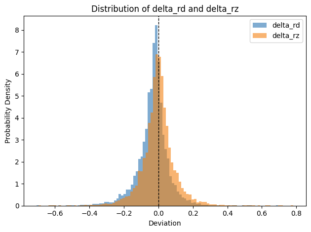
To demonstrate the numerical bias, we simulate the CDNA3 v_mfma_f32_32x32x8_f16 instruction with \(\Phi_\text{TR-FDPA}\) and a hypothetical v_mfma_f32_32x32x8_f16_rz instruction with modified \(\Phi_\text{TR-FDPA}'\) that replaces the RD operation in the internal fused summation with RZ. We generate random values from the standard normal distribution \(N(0,1)\) for \(C\), and the normal distribution \(1000\times N(0, 1)\) for \(A\) and \(B\). Then, we obtain the CDNA3 output \(D_\text{RD}=\Phi_\text{TR-FDPA}(A,B,C)\) and the output of the hypothetical instruction \(D_\text{RZ}=\Phi_\text{TR-FDPA}'(A,B,C)\). We also compute the real result \(D_\text{real}=A\times B+C\) using FP64, and compute \(\delta_\text{RD}=D_\text{RD}-D_\text{real}\) and \(\delta_\text{RZ}=D_\text{RZ}-D_\text{real}\). As Figure 14 shows, the distribution of \(\delta_\text{RD}\) is biased toward the negative direction while the distribution of \(\delta_\text{RZ}\) is symmetric.
6.3 Workaround and Mitigation Method↩︎
For software developers, we suggest avoiding the instructions with accuracy risks and using higher-precision alternative instructions instead. For example, if software uses NVIDIA MMA instructions with FP16 output, developers should switch to the FP32-output variant for better accuracy. If software uses FP8 MMA instructions on NVIDIA Ada Lovelace or Hopper architectures, computing the FP8 MMA with FP16 MMA instructions or migrating to Blackwell or RTX Blackwell architectures can restore full precision.
The numerical bias on AMD CDNA3 occurs when \(A\) and \(B\) contain large-magnitude numbers and the elements of \(C\) are negative numbers with relatively small magnitudes. Therefore, developers can use Matrix Cores only for matrix multiplication by setting \(C=0\), and use the general compute units for full FP32-precision matrix accumulation to mitigate this issue.
6.4 Suggestions for Future MMAU Design↩︎
For MMAU designers, the numerical accuracy of the hardware design should be carefully scrutinized. According to our modeling results, although different architectures adopt various arithmetic operations and configurations, most instructions have FP32-like numerical accuracy. To achieve this, hardware designers should avoid the designs in Table 10 and maintain FP32-level precision at every computational step. We also suggest adopting sign-and-magnitude or ones’ complement encoding internally because the two’s complement encoding is less suitable for implementing symmetric rounding modes.
7 Conclusion↩︎
This paper introduces the first bit-accurate models of the arithmetic behaviors of matrix multiply-accumulate units (MMAUs) from NVIDIA and AMD GPUs through our closed-loop feature probing (CLFP) approach. With the white-box models, we analyze the root causes of MMAU numerical discrepancies and numerical errors, providing insights into software mitigation and future hardware designs. This work is open-source, encouraging continuous testing, transparent numerical analysis, and accuracy-aware design space exploration.
References↩︎
For example, if the summation tree follows Figure 2 (a) and \(i=0\), \(j=1\), then the summation is computed as \(c+a_0b_0=v+U=U\), \(U+a_1b_1=U+-U=0\), \(0+a_2b_2=0+v=v\), and finally \(v+a_3b_3=v+v=2v\). Therefore, \(d^{(i,j)}/v=2\), representing that only two summands (i.e., \(a_2b_2\) and \(a_3b_3\)) are not swamped by \(p_i=a_0b_0\) and \(p_j=a_1b_1\).↩︎