Quantum Simulation of Non-Hermitian Special Functions and Dynamics via Contour-based Matrix Decomposition
January 01, 1970
Abstract
Simulating non-Hermitian dynamics on quantum computers is often hindered by the decay of success probability and the instability of non-diagonalizable matrices. Here, we present contour-based matrix decomposition (CBMD), a rigorous and versatile quantum functional calculus framework for simulating non-Hermitian matrix functions. By generalizing the matrix Cauchy residue theorem, CBMD decomposes holomorphic non-Hermitian operators into an analytic infinite contour-residue identity, followed by finite truncation with controlled error to yield linear combinations of Hermitian components. For first-order dynamics, CBMD achieves optimal query complexity across all parameters, strictly matching the optimal performance bounds within the linear combination of Hamiltonian simulation (LCHS) paradigm. Beyond first-order systems, the framework naturally generalizes to complex operator functions, including second-order wave dynamics and non-Hermitian special functions such as Bessel and Airy evolutions. Furthermore, CBMD systematically suppresses the asymptotic growth of non-Hermitian components, yielding a significant reduction in the required number of amplitude amplifications compared to the naive scheme of combining monomials via linear combination of unitaries (LCU) after Taylor expansion. Notably, CBMD avoids explicit dependence on matrix diagonalizability, effectively mitigating the long-standing challenges associated with ill-conditioned eigenvectors and Jordan blocks. Our work establishes a systematic matrix calculus that bridges high-performance classical numerics and fault-tolerant quantum algorithms. It should be noted that CBMD inherits standard LCU overheads, and requires the target function to have a bounded growth order on the real axis.
1 Introduction↩︎
Quantum computing has emerged as a transformative paradigm across physics and computer science, offering computational capabilities that fundamentally outperform classical algorithms in solving linear systems [1], [2], unstructured search [3], and the simulation of quantum many-body systems [4]–[6]. While evaluating functions of Hermitian matrices and simulating unitary dynamics represent a natural fit for quantum hardware, many frontier physical and mathematical problems require evaluating complex holomorphic functions of non-Hermitian operators. Such non-Hermitian matrix functions are ubiquitous; they are not only the foundation for simulating dissipative open quantum systems but also serve as direct analytical solutions to a vast array of matrix differential equations [7], [8], [8], [9], [9]–[19].
The advent of quantum singular value transformation (QSVT) has resolved a multitude of problems related to matrix function evolution and solving. Based on polynomial expansions, QSVT achieves optimal performance across various metrics [20]. However, performing general functional transformations on the matrix itself rather than on its singular values and is equally crucial. This class of problems encompasses matrix polynomials, quantum system simulations, and matrix differential equations [21]. Transformations on matrix functions can be directly understood as applying functions to eigenvalues rather than singular values. The most prominent example is quantum eigenvalue processing (QEP), an algorithm that is inherently sensitive to matrix diagonalizability and the condition number of the eigenvector matrix [22], [23]. Similarly, matrix contour integrals, inspired by classical heuristic matrix functional calculus, have been directly applied to quantum algorithms [24], [25]. By leveraging the powerful parallel capabilities of quantum computers and existing matrix inversion algorithms, these methods have achieved excellent query complexities for matrix functions and yielded good results on general problems like matrix polynomials [26]–[28]. Nevertheless, these approaches still fail to circumvent the reliance on eigenvector condition numbers and remain primarily suited for diagonalizable matrices. Although the universality of the LCU method allows it to be extended to matrix addition and multiplication without depending on condition numbers, direct monomial linear combinations based on LCU often suffer from exponentially exploding \(L_1\)-norms and exorbitantly high query costs [22], [29], [30].
For a specific example of matrix functions, namely the exponential function \(e^{-At}\), significant progress has been made recently. The Schrödingerization [9], [13], [14], [31] and LCHS [8], [11], [32] methods have realized the evolution of arbitrary matrices \(A\) from different perspectives. Notably, their algorithmic complexities do not depend on the eigenvector condition number of matrix \(A\), thereby achieving optimal complexity and fundamentally optimizing this specific problem. Furthermore, utilizing LCU and block-encoded matrix multiplication, these methods can be readily generalized to matrix operations involving addition and multiplication, such as trigonometric functions. We observe that the underlying mathematical principles of these two algorithms are quite similar. Inspired by the LCHS method, we clearly and naturally extend this framework to a wide array of special functions, achieving seamless integration with existing quantum computing frameworks.
In this work, we propose CBMD method, a rigorous and universal quantum functional calculus framework that fundamentally generalizes the treatment of exponential functions to a broad class of holomorphic functions exhibiting stable modulus growth along the real axis. Instead of relying on error-prone numerical quadrature or expensive resolvent block-encoding, CBMD generalizes the matrix Cauchy residue theorem to directly decompose holomorphic non-Hermitian operator functions into exact infinite contour-residue identity, followed by finite truncation with controlled error [33]. Each resulting Hermitian component can subsequently be implemented independently and efficiently via standard QSVT. This approach helps evaluate non-Hermitian functions while effectively mitigating the reliance on matrix diagonalizability and condition numbers.
The primary advantage of the CBMD framework becomes evident when applied to target functions that exhibit asymptotic stability or bounded moduli along the real axis. By constructing entire auxiliary functions that mirror the analytic structure of the target function, CBMD systematically suppresses the asymptotic growth of non-Hermitian components across the complex plane. Consequently, as demonstrated in our subsequent applications, CBMD improves the exponential dependence from \(\mathcal{O}(e^{t\sqrt{\|A\|}})\) to \(\mathcal{O}(e^{t\sqrt{\|H\|/2}})\) under the stated assumptions, thereby significantly reducing the simulation overhead.
In achieving optimal query complexity for first-order non-unitary dynamics, our approach matches the best complexity scaling when compared to algorithms under the LCHS framework [8], [11], [32]. While recent optimizations in time-dependent Hermitian evolution have yielded algorithms that surpass all complexity bounds within the LCHS framework, which providing inspiration for our future work and CBMD already excels in evaluating complex non-Hermitian special functions, including second-order non-Hermitian wave dynamics, non-Hermitian Bessel dynamics, and symmetry non-Hermitian Airy functions [21]. In these regimes, targeting real axis stability allows CBMD to strictly bound the \(L_1\) norm of the LCU coefficients, yielding a systematic exponential reduction in amplitude amplification overhead compared to naive polynomial expansions combined with LCU.
Ultimately, by replacing numerical approximations with an exact discrete contour series, CBMD establishes a unifying and highly scalable matrix calculus on quantum computers. It shifts the paradigm of non-Hermitian quantum algorithms from algebraic manipulations at the matrix level to \(\mathbb{Z}_3\) root-of-unity decompositions in the complex plane, paving the way for efficient quantum exploration of non-Hermitian physics and real-world system solving and computational applications.
While CBMD provides a versatile matrix calculus, it is important to clearly outline its algorithmic boundaries. The framework inherently inherits QSVT and LCU overheads, including necessary norm bounds for state preparation. Furthermore, the framework relies on constructing analytic bounding envelopes on the complex plane, making it currently difficult to apply to target functions with a growth order exceeding one.
2 Contour-based matrix decomposition↩︎
Due to the well-behaved spectral decomposition properties of Hermitian matrices, functional transformations applied to them can inherently be viewed as functions acting on their spectra. These properties essentially guarantee that mapping a Hermitian matrix only requires addressing a mapping over the set of real numbers [8]. Consequently, evaluating functions of Hermitian matrices is significantly more tractable than that of general matrices, in both classical and quantum computing paradigms. In the quantum domain, in particular, QSVT can be directly applied to evaluate functions of Hermitian matrices. Our primary motivation, therefore, lies in transforming the general matrix function problem into a Hermitian matrix function problem, allowing us to directly leverage these powerful existing computational methods.
The idea behind the CBMD framework draws inspiration from Cauchy’s integral theorem in complex analysis [33]. It establishes a fundamental link between the value of a closed contour integral in the complex plane and the sum of the residues of the poles enclosed by that contour, thereby simplifying the evaluation of such integrals. A cornerstone of the theorem is that the integral of a holomorphic function along a simple closed contour vanishes. For meromorphic functions possessing poles within the contour, techniques such as keyhole contours can transform the original integral into integrals around infinitesimal circles enclosing each pole [33]. This allows the analysis to focus on local behavior near singularities, thereby circumventing the complexity of the original integration path.
To provide a rigorous basis for our framework, we briefly review the extension of Cauchy’s residue theorem to matrix-valued functions, as established in the Riesz-Dunford functional calculus [34]. By interpreting a matrix as an array of scalar complex functions, the contour integration of a matrix function \(F(z)\) is defined element-wise, with each entry integrated independently along the contour. For completeness, we state the following standard result:
Lemma 1 (Matrix Residue Theorem). Let \(\Gamma\) be a simple closed contour and \(F(z)\) a matrix-valued function whose entries are meromorphic inside \(\Gamma\). If \(\{z_k\}\) are the simple 1-order poles of \(F(z)\) enclosed by \(\Gamma\), then \[\oint_\Gamma F(z) \,\mathrm{d}z = 2\pi i \sum_{k} \mathrm{Res}(F, z_k),\] where \(\mathrm{Res}(F, z_k)\) denotes the matrix of element-wise residues at pole \(z_k\).
Utilizing this technical lemma, we now derive the core decomposition identifying the relationship between holomorphic transformations of non-Hermitian and Hermitian matrices. Specifically, consider the aforementioned non-Hermitian matrix \(A= i H+L\) and a target holomorphic function \(f\) in the region enclosed by \(\Gamma\), here \(H^\dagger=H\) and \(L^\dagger=L\). We introduce holomorphic functions \(h_1(z)\) with real zeros \(\{q_r\}\) and an auxiliary holomorphic function \(h_2(z)\) with non-real zeros \(\{p_r\}\).
Then considering the matrix-valued function \[F(z) = \frac{h_{1}( i )h_{2}( i )f({zH+L})}{(z- i )h_1(z)h_2(z)},\] whose poles is \(S = \{ i \}\cup\{p_r\}\cup\{q_r\}\), applying Lemma 1 gives \[\underbrace{\frac{1}{2\pi i }\oint_\Gamma F(z) \,dz}_{\text{Integral Remainder \epsilon_\text{IR}}} =\underbrace{f( i H+L)}_{\text{Target Transformation}} + \underbrace{\sum_{s\in \{ q_r \}\subset \mathbb{R}}{c_sf(H_s)}}_{\text{Discrete Sampling (QSVT+LCU)}} + \underbrace{\sum_{s\in \{p_r\}}{c_sf(H_s)}}_{\text{Auxiliary-pole Error \epsilon_\text{AE}}}, \label{eq:lcf}\tag{1}\] where \(H_s=sH+L\) and \(c_s=\lim\limits_{z\rightarrow s}\frac{(z-s)h_{1}( i )h_{2}( i )}{(z- i )h_1(z)h_2(z)}\). Generally, the term \({\sum_{s\in \{ q_r \}\subset \mathbb{R}}{c_sf(H_s)}}\) can encompass an infinite series. For practical implementations, truncation must be considered, thereby introducing a controllable truncation error, as well as the error arising from the polynomial approximation used in QSVT.
Restricting to \(h_2(z)\) with only simple zeros \(\{p_r\}\) satisfying \(\{ p_r\} \cap \{ - i \}=\varnothing\), we can choose \(h_2(z)\) and \(\Gamma\) so as to suppress both the integral remainder \(\epsilon_{\text{IR}}=\|\oint_{\Gamma} F(z)\mathrm{d}z\|\) and the auxiliary-pole error \(\epsilon_{\text{AE}}=\|\sum_{s\in\{p_r\} }c_s f( i H_s) \|\). It is worth noting that Eq. 1 admits multiple variant forms. For instance, one could alternatively construct the integral using \(f( i H+ i zL)\) and designate the target pole at \(z = - i\), among various other configurations. For the sake of clarity and exposition, we have chosen to present only one representative formulation here. Nevertheless, all such alternative variations are conceptually identical to Eq. 1 , sharing the exact same underlying mathematical rationale.
This procedure yields the decomposition of the target transformation \(f(A)\) into a linear combination of anti-Hermitian transformations \(\sum_{s\in\{q_r\}}c_s f( i H_s)\). Each term can be realized via Hamiltonian simulation, QSVT or quantum signal processing (QSP) techniques [20], [35], [36]. The target transformation \(f(A)\) is then synthesized using the LCU method [29], enabling quantum simulations.
In an ideal scenario, assuming that \(\epsilon_{\text{AE}}\) and \(\epsilon_{\text{IR}}\) represent vanishing error terms and \(\sum_{s\in \{ q_r \}}{|c_s|}\) converges to a fixed constant, the computational complexity of implementing \(\sum_{s\in \{ q_r \}}{c_sf(H_s)}\) is predominantly governed by the growth rate of \(\|f(H_s)\|=\|f(sH+L)\|\), where \(s \in \mathbb{R}\). Typically, since \(\sum_{s\in \{ q_r \}}{c_sf(H_s)}\) represents an infinite series rather than a finite sum, evaluating \(f(H_s)\) inevitably involves arbitrarily large values of \(s\). Because \(H_s\) is a purely Hermitian operator, which meaning its spectrum lies entirely on the real line and it is crucial that the function’s modulus \(|f(z)|\) does not exhibit rapid growth for real \(z\). If \(|f(z)|\) were to diverge aggressively along the real axis, synthesizing the target matrix function would demand excessively large LCU coefficients \(\sum_s c_s \|f(H_s)\|\), thereby fatally inflating the amplitude amplification overhead.
The fundamental reason this decomposition succeeds so remarkably for functions such as \(f(z) = e^{ i z}\) is precisely because its modulus remains strictly bounded and constant (\(|e^{ i z}| = 1\)) for all \(z \in \mathbb{R}\) [8], [11], [32]. Guided by this macroscopic intuition regarding real-axis stability, we have successfully generalized and applied this framework to a broader class of complex functions in the subsequent sections.
To provide a rigorous foundation for our complexity analysis and fully address the algorithmic implementation of Eq. 1 , we explicitly construct the hierarchical quantum circuits. We assume access only to the block-encoding of the general non-Hermitian matrix \(A = L + i H\), rather than separate oracles for \(H\) and \(L\).
We assume access to a unitary \(U_A\) acting on \(a_0 + n\) qubits, which provides an \((\alpha_A, a_0, \epsilon_0)\)-block-encoding of \(A\). Specifically, \[(\langle 0|^{a_0} \otimes I) U_A (|0\rangle^{a_0} \otimes I) = \frac{A}{\alpha_A}.\] Its inverse, \(U_A^\dagger\), naturally provides a block-encoding for \(A^\dagger/\alpha_A\).
For any real sampling pole \(s \in \mathbb{R}\), we must construct the block-encoding of the Hermitian combination \(M_s = sH + L\). Using the relations \(L = (A + A^\dagger)/2\) and \(H = (A - A^\dagger)/(2i)\), we analytically decompose \(M_s\) into a linear combination of \(A\) and \(A^\dagger\): \[M_s = s \left(\frac{A - A^\dagger}{2i}\right) + \frac{A + A^\dagger}{2} = \underbrace{\left(\frac{1-is}{2}\right)}_{c_0} A + \underbrace{\left(\frac{1+is}{2}\right)}_{c_1} A^\dagger.\] To implement this via a Linear Combination of Unitaries (LCU), we note that the \(L_1\)-norm of the coefficients is \(\alpha_{L1} = |c_0| + |c_1| = \sqrt{1+s^2}\). We define a 1-qubit state preparation oracle \(P_s\) that prepares the amplitudes and phases: \[P_s |0\rangle = \frac{1}{\sqrt{\alpha_{L1}}} \left( \sqrt{|c_0|}e^{i\arg(c_0)} |0\rangle + \sqrt{|c_1|}e^{i\arg(c_1)} |1\rangle \right) = \frac{1}{\sqrt{2}} \left( e^{-i\phi} |0\rangle + e^{i\phi} |1\rangle \right),\] where \(\phi = \arctan(s)\). The controlled-select oracle is simply \(S_{in} = |0\rangle\langle0| \otimes U_A + |1\rangle\langle1| \otimes U_A^\dagger\). The inner LCU unitary \(U_{sH+L} = (P_s^\dagger \otimes I) S_{in} (P_s \otimes I)\) thus yields an exact block-encoding of \(M_s\): \[(\langle 0|^{a_0+1} \otimes I) U_{sH+L} (|0\rangle^{a_0+1} \otimes I) = \frac{sH+L}{\sqrt{1+s^2}\alpha_A} \equiv \frac{M_s}{\alpha_s},\] where the new normalization factor is explicitly \(\alpha_s = \sqrt{1+s^2}\alpha_A\).
With the unconditionally stable Hermitian matrix \(M_s\) block-encoded by \(U_{sH+L}\), we directly apply standard QSVT. By invoking a polynomial \(P(x)\) of degree \(d\), QSVT yields a unitary \(V_s\) that block-encodes the function \(f(sH+L)\).
Finally, we synthesize the target evaluation using the truncated discrete sum from our contour identity: \(f(A) \approx \sum_{k=1}^K w_k f(s_k H + L)\). We employ a second LCU layer utilizing an auxiliary register \(|k\rangle\) of size \(\lceil \log_2 K \rceil\). The outer state preparation oracle \(P_{out}\) is defined as: \[P_{out} |0\rangle = \frac{1}{\sqrt{\alpha_{out}}} \sum_{k=1}^K \sqrt{|w_k|} e^{i\arg(w_k)} |k\rangle, \quad \text{where } \alpha_{out} = \sum_{k=1}^K |w_k|.\] Coupled with the outer select oracle \(S_{out} = \sum_{k=1}^K |k\rangle\langle k| \otimes V_{s_k}\), the final unitary operation \[U_{final} = (P_{out}^\dagger \otimes I) S_{out} (P_{out} \otimes I)\] produces the block-encoding of \(f(A)/\alpha_{out}\). The success probability of this overarching LCU scheme is strictly bounded by the total normalization \(\alpha_{out}\), dictating the required amplitude amplification overhead explicitly analyzed in our subsequent wave, Bessel, and Airy theorems.
3 Application I: First-Order Non-Unitary Dynamics↩︎
Consider the dynamics of a vector \(u(t)\) governed by a linear ordinary differential equation (ODE): \[\label{eqn:ODE} \frac{\mathrm{d} u(t)}{\mathrm{d} t} = -A(t) u(t) + b(t), \quad u(0) = u_0.\tag{2}\] Since inhomogeneous equations with \(b(t)\not\equiv 0\) can be mapped to an equivalent homogeneous form [9], [13], [14], we then focus on solving Eq. 2 in the case of \(b(t)\equiv 0\). This case yields the solution \[\label{eqn:s95hODEs} u(t) = \mathcal{T}\mathrm{e}^{-\int_0^t A(s) \mathrm{d} s} u_0,\tag{3}\] where \(\mathcal{T}\) is the time ordering operator. It has wide applications, including simulating imaginary time evolution [37], [38], open quantum systems [39], [40], computational fluid dynamics [41], and finance [42].
Then applying the CBMD framework to simulate non-unitary dynamics described in Eq. 2 , we set appropriate auxiliary functions \(h_1(z)\) and \(h_2(z)\) such that the integral remainder \(\epsilon_{\text{IR}}\) vanishes. This effectively decomposes the non-Hermitian evolution into a linear combination of Hermitian evolutions. This conversion is formalized below, with proof provided in the Appendix 7.
Lemma 2 (Matrix Series Identity). Let \(A(t) = L(t) + i H(t)\), where \(H(t)\) and \(L(t)\) are Hermitian and \(L(t)\succeq 0\). Let \(a\in\mathbb{R}\) such that \(\| \int_{0}^{T}L(s) \,\mathrm{d} s\| \leq 2\pi a\), and \(\{p_r\}_{r=1}^m\) be a set of complex numbers satisfying \(\{p_r\}_{r=1}^m\cap \{- i \}=\varnothing\) and \(\{p_r\}_{r=1}^m\cap \{ \mathbb{Z}/a \} = \varnothing\). Then the following identity holds: \[\begin{align} \label{series95MSI} &\underbrace{{\mathcal{T}\mathrm{e}^{-\int_{0}^{T}A(s)\mathrm{d}s}}}_\text{Target} -\underbrace{\frac{1}{a}\sum_{k\in \mathbb{Z}}\frac{({\mathrm{e}^{-2\pi a}-1})\mathcal{T}\mathrm{e}^{- i \int_{0}^{T}(H(s)+\frac{k}{a}L(s))\mathrm{d}s}}{2\pi i (\frac{k}{a}+ i ) \left[\prod_{r=1}^{m}\frac{{k}/{a}-p_{r}}{- i -p_{r}}\right]} }_{\text{Linear Combination of Hamiltonian Simulation (LCHS)}} \\ &\underbrace{ -\sum_{r=1}^{m}\frac{{(\mathrm{e}^{-2\pi a}-1)}\mathcal{T}\mathrm{e}^{- i \int_{0}^{T}H(s)+p_{r}L(s)\mathrm{d}s}}{(\mathrm{e}^{-2\pi p_{r} a i }-1)\prod_{r^{\prime}\neq r}^{m}{\frac{p_r-p_{r^{\prime}}}{- i -p_{r^{\prime}}}}}}_{\text{Auxiliary-pole Error}}=\underbrace{0}_{\epsilon_{IR}}. \end{align}\tag{4}\]
Optimizing the LCU implementation involves a critical trade-off in the selection of the auxiliary poles \(\{p_r\}\). The pole placement must balance three competing factors affecting the LCU procedure’s complexity: the number of LCU terms, the simulation cost of each term, which depends on the spectral norm, and the overall success probability is inversely proportional to the square of the sum of the coefficient magnitudes. A high pole density (small \(|p_r - p_{r'}|\)) inflates the coefficients, degrading the success probability. Conversely, sparse poles may necessitate a larger summation range to control the truncation error, thus increasing complexity. By carefully selecting \(\{p_r\}\) and adaptively scaling their number \(m\) with the desired precision \(\epsilon\), we obtain a fast-converging LCU series, summarized in the following theorem, which achieves an optimal query complexity and a success probability lower-bounded by a constant of \({\|u_{0}\|}/{\|u_{T}\|}\), here \(u_{T}:=u(T)\).
Lemma 3 (Fast-Converging LCU Series). There exists a LCU \(\sum_{j}{c_{j}U_{j}}\) approximating \(\mathcal{T}\mathrm{e}^{-\int_{0}^{T}A(s)\mathrm{d}s}\) within error \(\epsilon_{1}\), where \(U_{j} = \mathcal{T}\mathrm{e}^{ i \int_{0}^{T}(H(s)+k'_{j}L(s))\mathrm{d}s}\), \(k'_{j}\in \mathbb{R}\). The number of distinct unitaries \(U_{j}\) scales \(\mathcal{O}\left(\log\frac{1}{\epsilon_{1}}(\log\frac{1}{\epsilon_{1}} + a)\right)\) and \(\| \int_{0}^{T}L(s)\, \mathrm{d} s\| \leq 2\pi a\), the coefficient magnitudes obey \(\max_{j}|k'_{j}| \in \mathcal{O} \left({\log(1/\epsilon_{1})}\right)\), and the total weight satisfies \(\sum_{j}{|c_{j}|}\in {\mathcal{O}}(1)\).
Lemma 3, proven in the Appendix 8, allows for the direct approximation of the time-evolution operator \(\mathcal{T}\mathrm{e}^{-\int_0^T {A}(s) \mathrm{d}s}\) via a LCU \(\sum c_j {U}_j\). Each \(U_j\) corresponds to a Hermitian Hamiltonian \(H_j(s)=H(s)+k'_jL(s)\) and for time-independent cases, algorithms such as QSVT achieve precision \(\epsilon_1\) with query complexity \(\mathcal{O}(\|H_j\| T+{\log({1}/{\epsilon_1})})\) [20]. For time-dependent cases, a truncated Dyson series expansion yields \(\mathcal{O}(\|H_j\|T\frac{\log(\|H_j\|T/\epsilon_1)}{\log\log(\|H_j\|T/\epsilon_1)})\) [43], here \(\|H_j\|:=\max_t\|H_j(t)\|\). The overall cost is thus dominated by the largest \(|k'_j|\). The amplitude amplification procedure followed by the LCU method with overhead \(\|u_0\| / \|{u}_T\|\) results in the total precision \(\epsilon\) as \(\epsilon_1 = \epsilon \|{u}_T\| / \|u_0\|\), in which the total query complexity can be obtained. We present the results in the following theorem.
Theorem 1 (Non-Hermitian simulation via CBMD). The non-unitary dynamics in Eq. 2 with \(b(t)\equiv 0\) can be solved at time \(T\) with error \(\epsilon\) and \(\Omega(1)\) success probability, the query complexity for the block encoding inputs of matrix \(A(t)\) is approximately \[\widetilde{\mathcal{O}}\left(\frac{\|u_0\|}{\|u_T\|}\alpha_{A}T{(\log\frac{1}{\epsilon})^2}\right)\] for the time-dependent case. And in the time-independent case, the query complexity of \(A\) is about \[\widetilde{\mathcal{O}}\left(\frac{\|u_0\|}{\|u_T\|}\alpha_{A}T\log\frac{1}{\epsilon}\right).\] The query complexity to the state preparation oracle for \(u_0\) is \(\mathcal{O}\left(\frac{\|u_0\|}{\|u_T\|}\right)\). The coefficients of the LCU procedure are approximately \(\mathcal{O}\left((\log\frac{u_r}{\epsilon} + \| \int_{0}^{T}L(s) \mathrm{d}s\|)\log\frac{u_r}{\epsilon}\right)\); thus, the complexity of the ancillary qubits is on the order of its logarithm, here \(L(t)=\frac{A(t)+A^\dagger(t)}{2}\).
To properly contextualize the performance of the CBMD framework, it is instructive to qualitatively compare its overall computational complexity with competing classical numerical methods. For an \(N\)-dimensional non-Hermitian system where \(N=2^n\), classical approaches such as exact diagonalization, Krylov subspace methods, or standard finite-difference time-domain algorithms generally incur a computational cost that scales polynomially with the system dimension \(N\) [44]. Consequently, the classical resource requirement grows exponentially with the number of qubits \(n\). In contrast, as established in our complexity theorems, the quantum query complexity of CBMD scales polynomially with \(n\), the evolution time \(T\), and \(\log(1/\epsilon)\), offering a potential exponential speedup in terms of system size. However, this quantum advantage is fundamentally conditioned on the non-unitary amplitude amplification overhead. In the efficient regime where the target state norm does not decay exponentially relative to the initial state, the exponential speedup over classical methods is fully realized. Conversely, if the state norm decays exponentially, the required amplification steps offset the dimensional advantage. This probability decay represents an intrinsic physical bottleneck rather than an algorithmic flaw, presenting a universal challenge for all quantum non-Hermitian simulation paradigms. Compared to the spectral method [15], our approach to non-Hermitian simulation does not rely on matrix diagonalizability or the Jordan condition number. Furthermore, in comparison with the truncated Dyson approach [18], our scheme eliminates a logarithmic factor and completely removes the dependence on time, matrix norm, and target error in the complexity of initial state preparation. Finally, in contrast to the time-marching scheme [45], our method exhibits a strictly linear, rather than quadratic, dependence on both the matrix norm and time.
In the realm of non-Hermitian simulation, CBMD inherits the LCHS framework and attains a query complexity matching that of optimal-LCHS within the class of LCHS-based algorithms [32]. A comparison of these recent advancements is presented in Table 1, and the analytical connections between Eq. 1 and existing LCHS methods are detailed in Appendix 9. It should be noted that CBMD primarily optimizes the kernel function without fundamentally altering the underlying quantum computing framework. Consequently, it cannot currently match the superior query complexity achieved by the recently proposed algorithm [46].
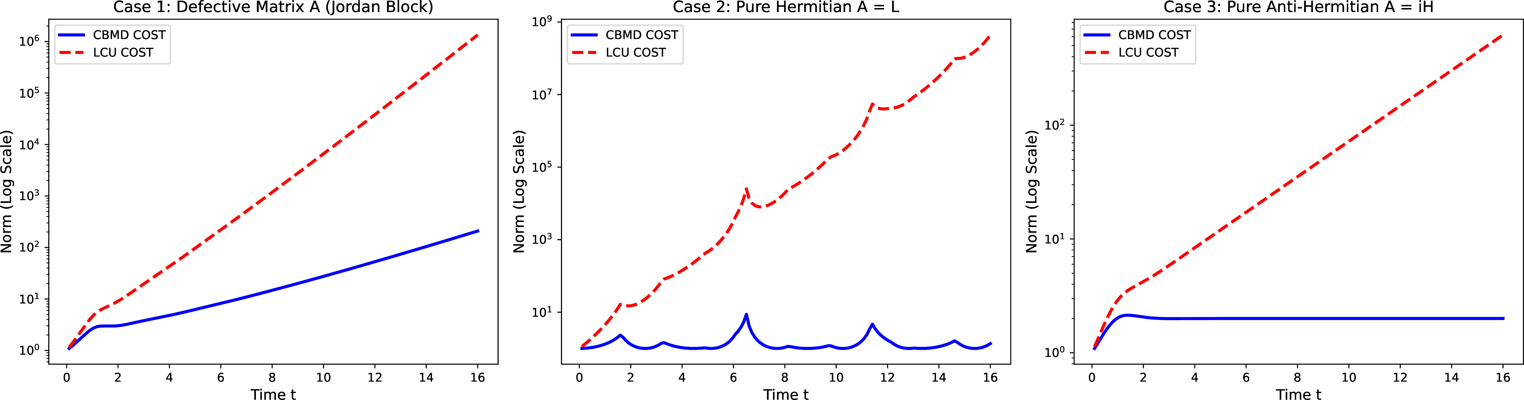
However, the primary advantage of CBMD lies in its broader versatility: it can be applied to evaluate a wider class of non-Hermitian matrix differential equations and provides a systematic approach for applications that remain challenging for traditional algorithms. Specifically, to evaluate and compare the number of amplitude amplifications required by CBMD in the case of a Jordan block, we perform a numerical test using a completely non-diagonalizable matrix \[iH+L = \left[ \begin{matrix} 1 & 2 \\ 0 & 1 \end{matrix}\right],\] and numerically compare its cost against that of the naive LCU method, as illustrated in Fig. 1.

| Algorithms | Query to \(A(t)\) | Query to \(u_{0}\) |
|---|---|---|
| Origin LCHS [8] | \(\widetilde{\mathcal{O}}\left( \frac{\|u_0\|}{\|u_T\|} \alpha_{A}T \frac{1}{\epsilon} \right)\) | \(\mathcal{O}\left( \frac{\|u_0\|}{\|u_T\|}\right)\) |
| Improved LCHS [11] | \(\widetilde{\mathcal{O}}\left( \frac{\|u_0\|}{\|u_T\|} \alpha_{A}T (\log \frac{1}{\epsilon})^{1+o(1)} \right)\) | \(\mathcal{O}\left( \frac{\|u_0\|}{\|u_T\|}\right)\) |
| Optimal LCHS [32] | \(\widetilde{\mathcal{O}}\left( \frac{\|u_0\|}{\|u_T\|} \alpha_{A} T\log \frac{1}{\epsilon} \right)\) | \(\mathcal{O}\left( \frac{\|u_0\|}{\|u_T\|}\right)\) |
| CBMD | \(\widetilde{\mathcal{O}}\left( \frac{\|u_0\|}{\|u_T\|} \alpha_{A} T\log \frac{1}{\epsilon} \right)\) | \(\mathcal{O}\left( \frac{\|u_0\|}{\|u_T\|}\right)\) |
4 Application II: Second-Order Wave Dynamics↩︎
To demonstrate that the superiority of the CBMD framework extends well beyond first-order non-unitary simulations, we conduct verification on a non-trivial physical example: the non-Hermitian wave equation [47]. By directly targeting the analytical structure of the evolution operator, we show that CBMD yields advantages that far surpass naive linear combinations or generic polynomial approximations.
Consider the dynamics of a physical system governed by a second-order wave equation with non-conservative terms. The evolution of the state \(u(t)\) at an arbitrary time \(t > 0\) can be described by: \[\label{eq:wave} \frac{d^2}{dt^2}u(t) = -A u(t), \quad u(0) = u_0, \quad u'(0) = 0,\tag{5}\] where \(A = L + iH\) is a general non-Hermitian operator, with \(L, H \in \mathbb{C}^{N \times N}\) being Hermitian matrices and \(L\succ 0, H\succ 0\). The analytical solution at time \(t\) is given by the matrix wave propagator: \[\label{eq:analytical95solution} u(t) = \cos\left(\sqrt{A}t\right) u_0 = \cos\left(\sqrt{L + iH}t\right) u_0.\tag{6}\] Because the Taylor expansion of the cosine function consists exclusively of even powers, the branch cuts of the square root are naturally eliminated, rendering the operator \(\cos(\sqrt{A}t)\) an entire function globally well-defined on \(\mathbb{C}\). Our objective is to prepare a normalized quantum state \(|u(t)\rangle\) with a success probability of \(\Omega(1)\) and within a precision of \(\epsilon\).
To decompose this non-Hermitian function into an LCU composed of purely Hermitian arguments, we construct the following complex-valued auxiliary function parameterized by \(t\): \[F(z) = \frac{h(1) \cos\left(\sqrt{izH + L} \;t\right)}{h(z) \cdot z(z-1)},\] where \(h(z) = \cos\left(\sqrt{2\pi a i z} \;t\right)\).
To suppress the asymptotic growth of the numerator (\(\sim \exp(t\sqrt{\|H\||z|})\)), the scaling parameter \(a \in \mathbb{R}^+\) simply needs to satisfy \(2\pi a \geq \|H\|\); we can conveniently set \(2\pi a = \|H\|\) when the norm is known. The function \(h(z)\) is an entire function, and its reciprocal yields strictly simple poles. By applying Cauchy’s residue theorem over a contour extending to infinity, the sum of all residues vanishes: \(\sum \text{Res}(F, z_p) = 0\). By combining all the first-order poles, we arrive at the following exact LCU identity, where the truncation error terms are explicitly distinguished:
\[\label{eq:lcu95exact} \begin{align} \cos\left(\sqrt{A}t\right) = & \underbrace{h(1) \cos\left(\sqrt{L}t\right) - h(1) \sum_{k=0}^K d_k \cos\left(\sqrt{\frac{(k+1/2)^2\pi}{2a t^2}H + L} \;t\right)}_{\text{Quantum Circuit Implementation by QSVT+LCU}} \\ & - \underbrace{h(1) \sum_{k=K+1}^\infty d_k \cos\left(\sqrt{\frac{(k+1/2)^2\pi}{2a t^2}H + L} \;t\right)}_{\text{Truncation Error}}, \end{align}\tag{7}\] where the coefficients are given by: \[d_k = \frac{(-1)^k}{\frac{(k+1/2)\pi}{2} \left( 1 + i \frac{(k+1/2)^2\pi}{2a t^2} \right)}.\]
Based on the preceding analysis, we establish the following theorem (proof provided in Appendix 10):
Theorem 2 (Complexity of Non-Hermitian Wave Equation). Consider the dynamics of a physical system governed by a second-order wave equation with non-conservative terms \(A = L + i H\) by Eq. 5 , where \(L, H \in \mathbb{C}^{N \times N}\) are Hermitian matrices (\(L\succ 0, H\succ 0\)). To prepare a normalized quantum state \(|u(t)\rangle\) with a success probability of \(\Omega(1)\) and precision \(\epsilon\), the resulting query complexities to the quantum algorithm for matrix \(A\) and the state preparation oracle of \(|u_{0}\rangle\) are respectively: \[\mathcal{O}\left( {u_r\kappa t \log(\|H\|t)} \sqrt{\frac{u_r\|H\|\log(\|H\|t)}{\epsilon} } \right) \quad \text{and} \quad \mathcal{O}\left(u_r \log(\|H\|t) \right),\] where \[u_r := \frac{\|u_0\| e^{\sqrt{\frac{\|H\|}{2}}t}}{\| \cos(\sqrt{A}t)u_0\|},\] and \(\kappa = \max(\kappa_H, \kappa_L)\).
Although \(u_r\) introduces a non-negligible exponential scaling factor, it can be effectively absorbed by the denominator \(\|\cos(\sqrt{A}t)u_0\|\). This is mathematically justified because the supremum of this operator’s norm, achieved when \(L\) is a zero matrix, can be strictly bounded by \(e^{\sqrt{\frac{\|H\|}{2}}t}\). Practically, we first prepare a block-encoding of \(\cos(\sqrt{A}t)\), meaning the optimal operator constructed is \(\frac{\cos(\sqrt{A}t)}{\|\cos(\sqrt{A}t)\|}\). Thus, this norm absorption utilizing the tight upper bound acts as an unavoidable, intrinsic overhead of the quantum evolution itself.
Crucially, this analysis underscores the significant algorithmic improvement of the CBMD approach. Consider a direct baseline combining the LCU technique with a naive Taylor expansion (utilizing monomials of the block-encoding of matrix \(A\)). Directly applying LCU and amplitude amplification in that scenario, even disregarding the operational overhead of a single LCU step and yields an amplitude amplification requirement that scales as \(\mathcal{O}\left(\frac{e^{\sqrt{\|A\|}t}\|u_{0}\|}{\| \cos(\sqrt{A}t)u_0\|}\right)\). By selectively targeting the analytical structure, our CBMD method yields an improvement in this overhead factor. It successfully reduces the exponent from \(\sqrt{\|A\|}\) to \(\sqrt{\|H\|/2}\), thereby completely decoupling the amplitude amplification cost from the potentially massive Hermitian component \(L\).
Remark The query complexity established in Theorem 2 is polynomial in \(t\) and \(1/\epsilon\) provided that the amplification factor \(u_r\) remains bounded by \(poly(t, 1/\epsilon)\), this condition is satisfied when the initial state \(u_0\) has a significant projection onto the well conditioned eigenspace of the operator \(\cos(\sqrt{A}t)\). To illustrate this mathematically, we analyze two distinct asymptotic scenarios. First, assume the matrix \(A\) is purely Hermitian, namely \(A=L\) where \(\|H\|=0\). In this case, the exponential numerator of \(u_r\) explicitly reduces to \(1\). If \(u_0\) aligns with the eigenvector corresponding to the maximum eigenvalue of the purely oscillatory operator \(\cos(\sqrt{L}t)\), the denominator is optimally preserved, leading to a constant amplification overhead \(u_r = \mathcal{O}(1)\). Second, assume \(A\) possesses only an imaginary part, namely \(A=iH\). The eigenvalues of \(\sqrt{A}\) take the general form \(\sqrt{|\lambda_{H}|} e^{\pm i \pi/4}\), which contain nonzero real and imaginary components. Consequently, the operator \(\cos(\sqrt{A}t)\) exhibits exponential growth over time. The numerator of \(u_r\) contains an explicit exponential scaling factor to account for this maximal possible divergence. However, if \(u_0\) perfectly projects onto the maximum eigenvalue of \(\cos(\sqrt{A}t)\), the state norm in the denominator \(\|\cos(\sqrt{A}t)u_0\|\) grows at the exact same exponential rate. The exponential term in the numerator and the amplification of the state norm in the denominator perfectly cancel each other, resulting once again in \(u_r = \mathcal{O}(1)\) without any exponential bottleneck. Conversely, if the target state resides primarily in a decaying or suppressed subspace, \(u_r\) will grow exponentially. This reflects the intrinsic difficulty of general nonunitary simulation, a universal challenge shared by all LCHS based methods where the success probability is fundamentally limited by the norm ratio of the final and initial states.
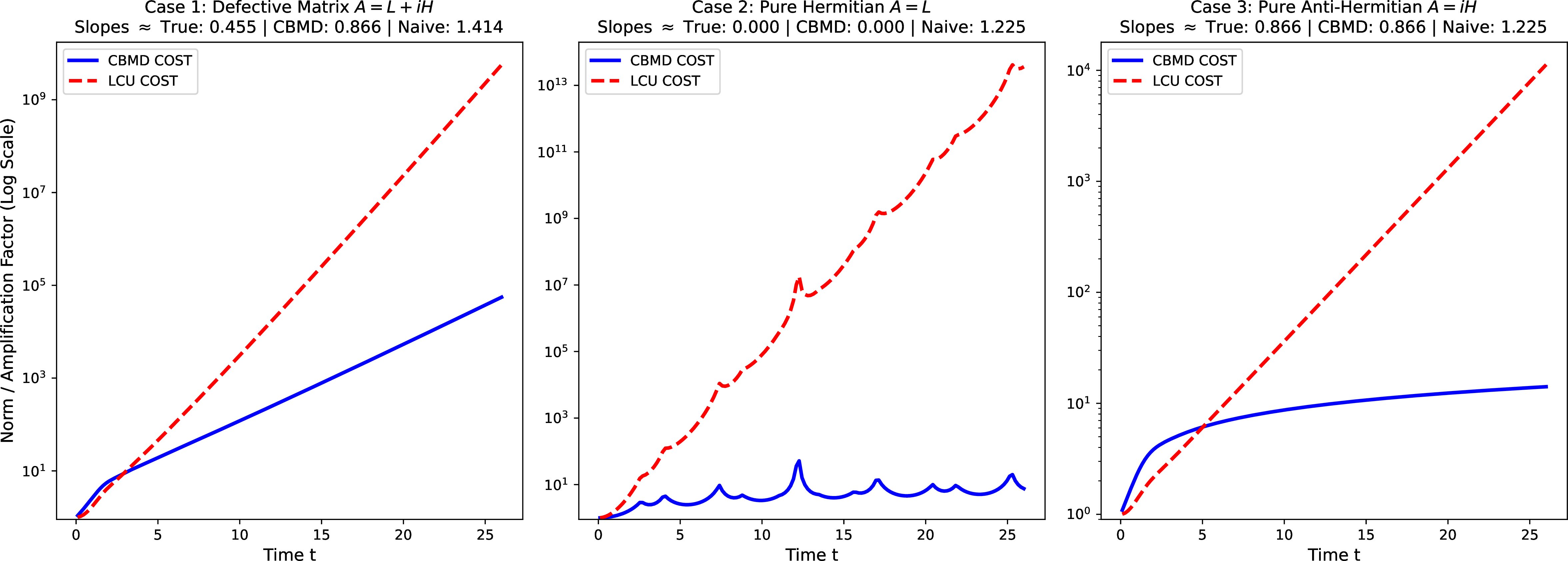
In the case of the wave function, we also evaluated the amplitude amplification cost corresponding to a completely non-diagonalizable matrix, which constitutes almost the entirety of the complexity cost. Due to the requirement of positive definiteness, we performed our tests using a completely non-diagonalizable matrix \[{i}H + L = \left[ \begin{matrix} 1+{i} & 1 \\ 0 & 1+{i} \end{matrix}\right],\] and numerically compared the cost against the naive LCU method, as illustrated in Fig. 2. This advantage achieved in the wave equation reveals a core mechanistic requirement for the CBMD framework: the success of the LCU decomposition hinges heavily on the asymptotic behavior of the target function. Functions corresponding to physical evolutions, such as \(e^{{i}z}\) or \(\cos(z)\), exhibit a stable and bounded modulus along the real axis. This fundamental stability is what allows us to deliberately construct entire auxiliary functions \(h(z)\) that perfectly neutralize the growth of the target function across the complex plane, keeping the \(L_1\)-norm of the resulting LCU coefficients tightly controlled and seamlessly scalable.
5 Application III: Non-Hermitian Special Functions↩︎
5.1 Non-Hermitian Bessel Dynamics↩︎
To demonstrate the versatility of the CBMD framework, we introduce a non-Hermitian dynamical differential equation governed by Bessel functions. Consider the matrix differential equation \[\label{eq:bessel} \frac{d^2u(t)}{dt^2} + \frac{1}{t} \frac{du(t)}{dt} + A u(t) = 0,\tag{8}\] subject to the initial conditions \(u(0) = u_0\) and \(u'(0) = 0\). Here, \(A = L + i H\) represents a general non-Hermitian operator, where \(L, H \in \mathbb{C}^{N \times N}\) are positive semi-definite Hermitian matrices (\(L\succ 0, H\succ 0\)).
This equation extends the traditional framework of constant dissipation dynamics by introducing a dynamical damping mechanism. Physically, it can be employed to model the evolutionary transition of an open system from an environment dominated regime to one governed by internal non-conservative dynamics. In the early stages of evolution (\(t \to 0\)), the system is subjected to strong decoherence from the external thermal bath, driven by the \(\frac{1}{t}\) damping term. As time progresses, this external constraint decays, allowing the system to gradually decouple from the environment, until the evolution is primarily dictated by the internal non-reciprocal interactions of \(A\). This mathematical structure is related to several physical scenarios, such as Hubble friction in the expansion of the early universe [48], time-dependent quenching in open quantum systems, and non-hermitian spatiotemporal optics [49]. Our CBMD framework provides a robust numerical approach to simulate these classes of matrix differential equations.
The analytical solution to this differential equation is directly given by the action of the zeroth-order Bessel function on the initial state, yielding \(u(t) = J_0(\sqrt{A}t)u_0\), where \[J_n(x) = \sum_{m=0}^{\infty} \frac{(-1)^m}{m! \Gamma(m+n+1)} \left(\frac{x}{2}\right)^{2m+n}.\] Recognizing that \(J_0(\sqrt{z})\) is an entire function, our algorithmic goal is to prepare the normalized final quantum state \(|u(t)\rangle \propto J_0(\sqrt{A}t)|u_0\rangle\) with a success probability of \(\Omega(1)\).
To enable the direct evaluation of this non-Hermitian operator function, we must systematically suppress its exponential divergence in the complex plane. We achieve this by defining an asymptotic regulator \(h(z) = \cos(\sqrt{2\pi a i z}t)\). By constructing the objective function \[F(z) = \frac{h(1) J_0(\sqrt{ i zH+L}t)}{h(z) z(z-1)},\] and evaluating its contour integral along a circular contour at infinity, we obtain an exact series expansion for the target dynamics: \[J_0(\sqrt{A}t) = h(1) J_0(\sqrt{L}t) - h(1) \sum_{k=0}^{\infty} d_k J_0\left( \sqrt{\frac{(k + 1/2)^2 \pi}{2a t^2} H + L} t \right),\] where the expansion coefficients are given by \[d_k = \frac{(-1)^k}{\frac{(k + 1/2)\pi}{2} \left( 1 + i \frac{(k + 1/2)^2 \pi}{2a t^2} \right)}.\] Setting aside truncation errors momentarily, the right-hand side of this expansion perfectly decomposes the non-Hermitian evaluation into a discrete sum of purely Hermitian operator functions. This form is inherently compatible with the LCU and QSVT frameworks. Furthermore, the rapid convergence of the Bessel function guarantees that the coefficients associated with the QSVT approximation remain highly tractable. These considerations culminate in the following theorem (proved in Appendix 11).
Theorem 3 (Complexity of Non-Hermitian Bessel Equation). Consider the dynamics of a physical system governed by the second-order wave equation with non-conservative terms \(A = L + i H\) as defined in Eq. 8 , where \(L, H \in \mathbb{C}^{N \times N}\) and \(L\succ 0, H\succ 0\). Assuming \(\|H\|\) is known, preparing the normalized quantum state \(|u(t)\rangle\) to precision \(\epsilon\) with a success probability of \(\Omega(1)\) incurs the following query complexities to the block-encoding of \(A\) and the state preparation oracle of \(|u_{0}\rangle\), respectively: \[\mathcal{O}\left( {u_r\kappa t \log(\|H\|t)} \sqrt{\frac{u_r\|H\|\log(\|H\|t)}{\epsilon} } \right) \quad \text{and} \quad \mathcal{O}\left(u_r \log(\|H\|t) \right),\] where the amplification factor \(u_r\) is defined as \[u_r := \frac{\|u_0\| e^{\sqrt{\frac{\|H\|}{2}}t}}{\| J_{0}(\sqrt{A}t)u_0\|},\]and \(\kappa = \max(\kappa_H, \kappa_L)\).
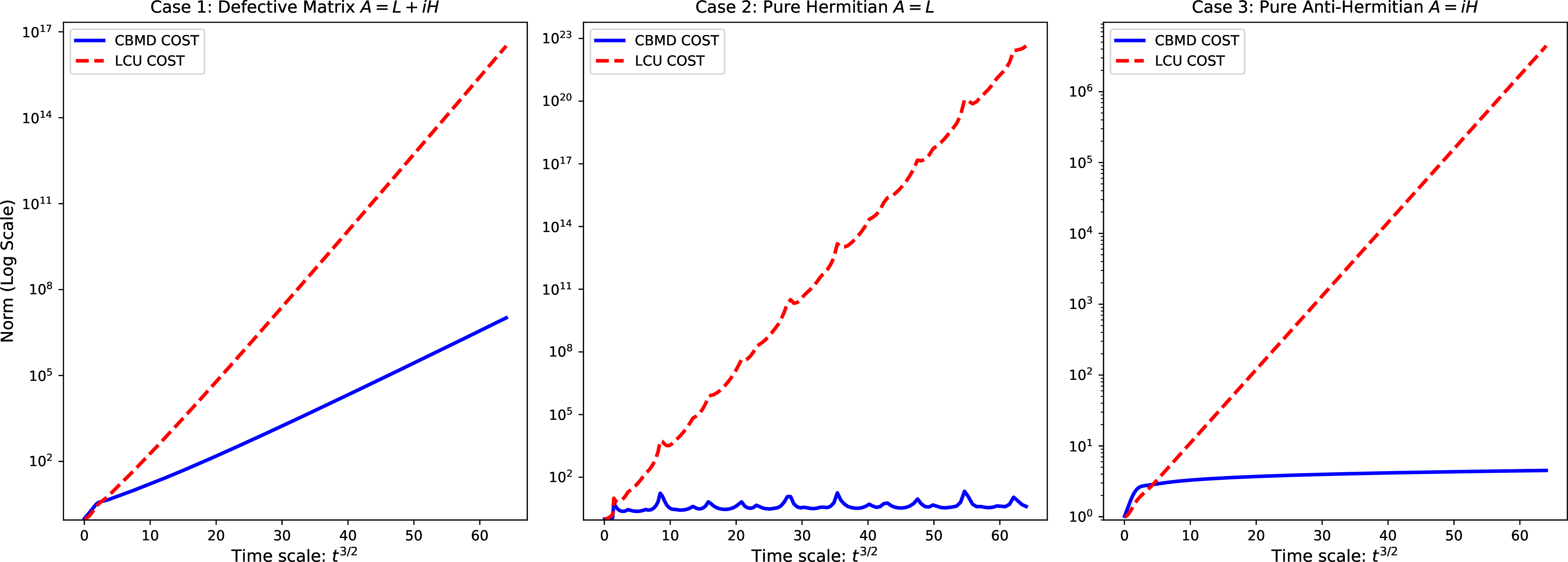
In the case of Bessel non-Hermitian dynamics, we similarly evaluated the amplitude amplification cost corresponding to a completely non-diagonalizable matrix, which dominates almost the entirety of the overall complexity. Due to the requirement of positive definiteness, we again employed a completely non-diagonalizable matrix \[{i}H + L = \left[ \begin{matrix} 1+{i} & 1 \\ 0 & 1+{i} \end{matrix}\right],\] for our test, and numerically compared the cost against the naive LCU method, as illustrated in Fig. 3. The complexity bounds in Theorem 3 characterize the underlying algorithmic mechanics of the CBMD framework for these Bessel dynamics. The numerator \(e^{\sqrt{t\|H\|/2}}\) in the amplification factor \(u_r\) serves as an analytic exponential envelope that accounts for the potential growth of the Bessel function in the complex plane. By rigorously bounding the \(L_1\) norm of the LCU coefficients using this envelope, CBMD effectively avoids the coefficient explosions typically associated with high degree polynomial approximations of non-Hermitian special functions. However, the overall efficiency of the algorithm is conditional upon the norm of the target state \(\|J_0(\sqrt{A}t)u_0\|\). In the efficient regime where the target state remains well-conditioned and its norm is not exponentially suppressed, the CBMD approach significantly reduces the amplitude amplification overhead compared to naive Taylor expansions. If the final state norm decays exponentially, the amplification factor \(u_r\) will grow accordingly, reflecting the fundamental probability decay inherent in simulating non-unitary special functions where the target state itself vanishes.
5.2 Non-Hermitian Airy Dynamics via \(\mathbb{Z}_3\) Symmetry Projection↩︎
As another mathematical test case for higher-order non-Hermitian evolution, we consider an idealized model of a parametric oscillator with a linearly varying generalized stiffness governed by the Airy equation: \[\label{eq:airy95new} \frac{d^2u(t)}{dt^2} + t A u(t) = 0,\tag{9}\] subject to the initial conditions \(u(0) = u_0\) and \(u'(0) = 0\). While treated here primarily as a formal mathematical model to demonstrate the algorithmic versatility of the CBMD framework, this equation is closely related to distinct physical regimes where a system undergoes a dynamical quench, amplifying the non-Hermitian coupling over time. Such mathematical structures are frequently employed to model phenomena such as accelerating wavepackets in parity-time-symmetric optics and dynamics near exceptional points [50].
Evaluating the exact scalar solution \(\mathrm{Ai}(A^{1/3}t)\) in the matrix domain presents severe analytical hurdles. The fractional power introduces ill-defined branch cuts, and the Airy function itself is an entire function of order \(3/2\). The latter causes the infamous Stokes phenomenon, inevitably leading to exponential divergence along closed contours and rendering standard Cauchy residue expansions impossible.
To circumvent these fundamental barriers, we introduce a \(\mathbb{Z}_3\) symmetry projection operator to construct a regularized propagator: \[f(z) = \frac{1}{3} \left( \mathrm{Ai}(-z) + \mathrm{Ai}(-\omega z) + \mathrm{Ai}(-\omega^2 z) \right),\] where \(\omega = e^{2\pi i /3}\). This \(\mathbb{Z}_3\) root-of-unity projection fundamentally alters the analytic structure by filtering out all powers except those of \(z^{3k}\). Consequently, the fractional roots perfectly annihilate, mapping \(f(A^{1/3}t)\) into an entire function of order \(1/2\) strictly dependent on \(A t^3\). All branch cuts vanish entirely, and the exact analytical solution to the dynamics is gracefully given by \(u(t) = \frac{f(A^{1/3}t)}{f(0)}u_0\).
To evaluate this target dynamics using the methodology established in the previous section, we define a trigonometric asymptotic regulator \(h(z) = \cos\left(\frac{2}{3} t^{3/2}\sqrt{ i \gamma z}\right)\). The \(2/3\) scaling perfectly matches the fundamental asymptotic growth of the filtered Airy envelope. By setting the bounding parameter \(\gamma \geq \|H\|\) and constructing the analogous objective function \[F(z) = \frac{h(1) f(( i zH+L)^{1/3}t)}{h(z) z(z-1)},\] the absolutely convergent contour integral as \(|z| \to \infty\) strictly vanishes.
The poles of the regulator correspond to the roots of the cosine function, aligning on the pure imaginary axis at \(z_k = - i \frac{9(k+1/2)^2\pi^2}{4\gamma t^3}\) for integers \(k \ge 0\). Substituting these into the non-Hermitian argument precisely cancels the imaginary unit, yielding a strictly converging series expansion free of branch cuts: \[f(( i H+L)^{1/3}t) = h(1) f(L^{1/3}t) - h(1) \sum_{k=0}^{\infty} d_k f\left( \left( L + \frac{9(k+1/2)^2\pi^2}{4\gamma t^3} H \right)^{1/3} t \right),\] where \(h(0) = \cos(0) = 1\) is absorbed naturally, and the explicitly evaluated residues are \[d_k = \frac{1}{h'(z_k) z_k (z_k - 1)} = \frac{(-1)^k}{\frac{(k+1/2)\pi}{2} \left( 1 + i \frac{9(k+1/2)^2\pi^2}{4\gamma t^3} \right)}.\]
Similar to the Bessel case, this expansion decomposes the intractable non-Hermitian evaluation into a discrete sum of unconditionally stable Hermitian operator functions, enabling direct application of LCU and QSVT quantum algorithms. And we give following Theorem 4 proved in Appendix 12.
Theorem 4 (Complexity of Non-Hermitian Airy Dynamics via \(\mathbb{Z}_3\) Projection). Consider the physical dynamics governed by the differential equation \(u''(t) + tAu(t) = 0\) with \(A = L + i H\) and initial condition \(u(0)=u_0, u'(0)=0\), where \(L, H \in \mathbb{C}^{N \times N}\) are Hermitian. Assuming \(\|H\|\) is known, preparing the normalized quantum state \(|u(t)\rangle\) to precision \(\epsilon\) with a success probability of \(\Omega(1)\) incurs the following query complexities to the block-encoding of \(A\) and the state preparation oracle of \(|u_{0}\rangle\): \[\mathcal{O}\left( {u_r\kappa t^{3/2} \sqrt{\|H\|}} \log\left(\frac{u_r t^{3/2} \sqrt{\|H\|}}{\epsilon}\right) \right) \quad \text{and} \quad \mathcal{O}\left(u_r t^{3/2} \sqrt{\|H\|} \right),\] where the amplification factor \(u_r\), characterizing the tightly filtered growth envelope of order \(1/2\), is defined as \[u_r := \frac{\|u_0\| \exp\left({\frac{2}{3} \sqrt{\frac{\|H\|}{2}t^3}}\right)}{\| f(A^{1/3}t)u_0\|},\] and \(\kappa = \max(\kappa_H, \kappa_L)\). Under ideal conditions where the terminal projection aligns with the principal eigenvector of the initial state \(u_0\) during prolonged evolution, the factor \(u_r\) remains effectively constant and functions as a dissipative term devoid of exponential decay.
In the case of Airy non-Hermitian dynamics, we similarly evaluated the amplitude amplification cost corresponding to a completely non-diagonalizable matrix, which dominates almost the entirety of the overall complexity. Since the algorithm ultimately outputs a normalized vector and the error metric evaluates the distance between normalized states, the overall algorithmic complexity inherently incorporates the amplification factor \(u_r\). Due to the requirement of positive definiteness, we again employed a completely non-diagonalizable matrix \[{i}H + L = \left[ \begin{matrix} 1+{i} & 1 \\ 0 & 1+{i} \end{matrix}\right]\] for our test, and numerically compared the cost against the naive LCU method, as illustrated in Fig. 4.
6 Discussion↩︎
A key conceptual breakthrough of this framework lies in the strategic introduction of asymptotic regulators to neutralize the exponential divergence of non Hermitian functions in the complex plane. By intentionally constructing entire auxiliary functions, such as the trigonometric envelope \(h(z)\) used in second order wave and Bessel dynamics, to match the analytic structure of the target dynamics, CBMD successfully bounds the \(L_1\) norm of the LCU coefficients. This mechanism elegantly bypasses the catastrophic coefficient explosion common in naive Taylor or polynomial approximations, thereby achieving a significant reduction in the required amplitude amplification overhead.
Furthermore, CBMD demonstrates remarkable robustness when confronting the deep analytic difficulties inherent in higher order non Hermitian physical models. By incorporating the \(\mathbb{Z}_3\) symmetric projection employed in Airy dynamics, the framework can eliminate fractional roots and completely remove ill conditioned branch cuts, mapping previously intractable non Hermitian evaluations into unconditionally stable Hermitian operator functions.
Although CBMD achieves outstanding optimization at the kernel function level, it currently operates within existing quantum computing frameworks like QSVT and LCU, and therefore unavoidably inherits certain fundamental quantum simulation overheads, such as the norm bounds required for state preparation. To fully mitigate the exponential dependence introduced by the amplitude amplification factor during long time evolutions, future implementations may need to incorporate time marching schemes. Concurrently, our research reveals that CBMD faces challenges in solving fractional order matrix functions, such as \(E_{\alpha}(-A)\) [51]. Moreover, when the growth order of \(f(z)\) exceeds 1, it becomes exceedingly difficult to find an appropriate \(h(z)\) to achieve global suppression of the growth of \(f(z)\). Based on the fundamental properties of complex variables, this limitation appears difficult to resolve strictly within the current CBMD framework.
Looking ahead, this foundational work opens several profound interdisciplinary research directions. Theoretically, one could further explore constructing discrete series representations using higher order poles to achieve faster convergence, or systematically optimizing auxiliary functions for systems with highly complex spectral topologies. The proposal of CBMD was tailored to leverage the compatibility of the QSVT algorithm with Hermitian matrix functions in quantum computing, while effectively integrating with the existing LCU framework. Distinct from functional matrix calculus, this method originates from classical theory and then radiates outward to empower quantum computing. To date, it remains an open question whether CBMD can improve classical matrix operations in a manner akin to matrix functional calculus, such as replicating the success of the AAA algorithm on coefficient matrices, or combining classical matrix functional theory to transform matrix \(A\) in the resolvent \(1/(zI-A)\) into a Hermitian matrix [52].
Acknowledgements↩︎
This work has been supported by the National Key Research and Development Program of China (Grant No. 2023YFB4502500).
Declarations↩︎
The authors declare that they have no conflict of interest.
This manuscript has no associated data.
7 Proof of Matrix Series Identity Lemma 2↩︎
Proof. Before proving the theorem, we establish a bound on the spectral norm of the time-ordered exponential. Let \(H(t)\) and \(L(t)\) be time-dependent Hermitian operators, \(\int_{0}^{t}L(s)ds\succeq 0\) and \(z\) is a real number. The evolution operator \(U(z) = \mathcal{T}\mathrm{e}^{\int_{0}^{t} ( i H(s) + zL(s)) \mathrm{d}s}\) is entire function [32], and has its spectral norm bounded by: \[\label{norm95len1} \|U(z)\| \le \exp\left(z \bigg{\|}\int_{0}^{t}L(s)ds \bigg{\|}\right),\tag{10}\] for \(\operatorname{Re}(z)\geq0\). As for \(\operatorname{Re}(z)<0\), \(U(z)\) has its spectral norm bounded by 1.
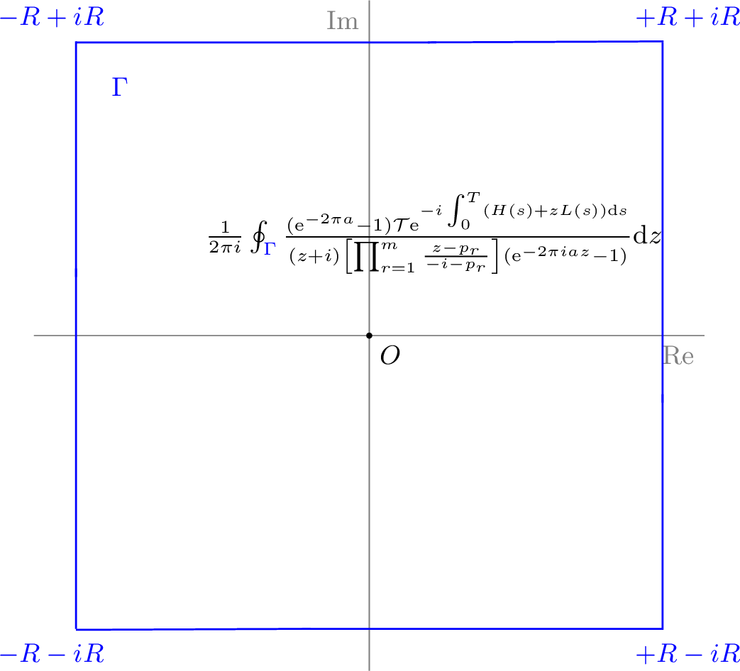
We now consider a large square contour in the complex plane, with vertices at \(\{\pm R\pm i R\}\), where \(R=(2N+1)/(2a)\to\infty\) as \(N\to\infty\) (\(N\in \mathbb{Z}^{+}\)), as shown in Fig. 5. Let this positively oriented contour be denoted as \(\Gamma\), and consider the following integral: \[\begin{align} \label{int95main} \frac{1}{2\pi i }\oint_{\Gamma} \frac{({\mathrm{e}^{-2\pi a}-1})\mathcal{T}\mathrm{e}^{- i \int_{0}^{T}(H(s)+zL(s))\mathrm{d}s}}{(z+ i )\left[ \prod_{r=1}^{m}\frac{z-p_{r}}{- i -p_{r}} \right](\mathrm{e}^{-2\pi i az}-1)}\mathrm{d}z. \end{align}\tag{11}\] We now partition the integral into four segments for estimation. We treat each element of the matrix as an independent function for integration. Furthermore, for a matrix \(M\), its spectral norm \(\|M\| \to 0\) if and only if each of its entries \(M_{ij} \to 0\). In the subsequent contour analysis, we will not make a detailed distinction between these two equivalent conditions. The first segment corresponds to the range of \(z\) from \(- i R - R\) to \(- i R + R\): \[\begin{align} &\Bigg{\|}\frac{1}{2\pi i }\int_{- i R - R}^{- i R + R} \frac{{(\mathrm{e}^{-2\pi a}-1)}\mathcal{T}\mathrm{e}^{- i \int_{0}^{T}(H(s)+zL(s))\mathrm{d}s}}{(z+ i )\left[ \prod_{r=1}^{m}\frac{z-p_{r}}{- i -p_{r}} \right] (\mathrm{e}^{-2\pi i az}-1)} \mathrm{d}z\Bigg{\|} \\ =&\Bigg{\|}\frac{R}{2\pi i }\int_{-1}^{1} \frac{{(\mathrm{e}^{-2\pi a}-1)}\mathcal{T}\mathrm{e}^{\int_{0}^{T}(- i H(s)-( i uR+R)L(s))\mathrm{d}s}}{(uR- i R+ i )\left[\prod_{r=1}^{m}\frac{uR- i R-p_{r}}{- i -p_{r}} \right] (\mathrm{e}^{-2\pi Ra- 2\pi i auR}-1)} \mathrm{d}u\Bigg{\|}\\ \leq&\frac{R}{2\pi (R-1)}\Bigg{\|}\int_{-1}^{1} \frac{\mathcal{T}\mathrm{e}^{\int_{0}^{T}(- i H(s)-( i uR+R)L(s))\mathrm{d}s}}{\left[\prod_{r=1}^{m}\frac{uR- i R-p_{r}}{- i -p_{r}} \right] (\mathrm{e}^{-2\pi Ra- 2\pi i auR}-1)} \mathrm{d}u\Bigg{\|}\\ \approx &\frac{R}{2\pi (R-1)}\Bigg{\|}\int_{-1}^{1} \frac{\mathcal{T}\mathrm{e}^{\int_{0}^{T}(- i H(s)-( i uR+R)L(s))\mathrm{d}s}}{\prod_{r=1}^{m}\frac{uR- i R-p_{r}}{- i -p_{r}} } \mathrm{d}u\Bigg{\|}\\ \leq &\frac{R}{2\pi (R-1)}\Bigg{\|}\int_{-1}^{1} \frac{1}{\prod_{r=1}^{m}|\frac{uR- i R-p_{r}}{- i -p_{r}}| } \mathrm{d}u\Bigg{\|}\\ \sim &\mathcal{O}(R^{-m})\to 0, \quad \text{for } u\in (-1, 1), R\to +\infty, m\geq 1. \end{align}\] The second segment corresponds to the range of \(z\) from \(- i R + R\) to \(i R + R\): \[\begin{align} &\Bigg{\|}\frac{1}{2\pi i }\int_{- i R + R}^{ i R + R} \frac{({\mathrm{e}^{-2\pi a}-1})\mathcal{T}\mathrm{e}^{- i \int_{0}^{T}(H(s)+zL(s))\mathrm{d}s}}{(z+ i )\left[ \prod_{r=1}^{m}\frac{z-p_{r}}{- i -p_{r}} \right] (\mathrm{e}^{-2\pi i az}-1)} \mathrm{d}z\Bigg{\|}\\ =&\Bigg{\|}\frac{R}{2\pi i }\int_{-1}^{1} \frac{({\mathrm{e}^{-2\pi a}-1})\mathcal{T}\mathrm{e}^{\int_{0}^{T}(- i H(s)+(uR- i R)L(s)) \mathrm{d}s}}{(uR i +R+ i )\left[\prod_{r=1}^{m}\frac{uR i +R i -p_{r}}{- i -p_{r}} \right] (\mathrm{e}^{2\pi auR-2\pi i aR }-1)} \mathrm{d}u\Bigg{\|}\\ \leq&\frac{1}{2\pi }\Bigg{\|}\int_{-1}^{1} \frac{\mathcal{T}\mathrm{e}^{\int_{0}^{T}(- i H(s)+(uR- i R)L(s)) \mathrm{d}s}}{\left[\prod_{r=1}^{m}\frac{uR i +R i -p_{r}}{- i -p_{r}} \right] (\mathrm{e}^{2\pi auR-2\pi i aR }-1)} \mathrm{d}u\Bigg{\|}\\ =&\frac{1}{2\pi (\mathrm{e}^{2\pi auR}+1)}\Bigg{\|}\int_{-1}^{1} \frac{\mathcal{T}\mathrm{e}^{\int_{0}^{T}(- i H(s)+(uR- i R)L(s)) \mathrm{d}s}}{\left[\prod_{r=1}^{m}\frac{uR i +R i -p_{r}}{- i -p_{r}} \right]} \mathrm{d}u\Bigg{\|}\\ \leq&\frac{1}{2\pi (\mathrm{e}^{2\pi auR}+1)}\int_{-1}^{1} \frac{\mathcal{T}\mathrm{e}^{R \| \int_{0}^{T}L(s) \mathrm{d}s\|}}{\prod_{r=1}^{m}|\frac{uR i +R i -p_{r}}{- i -p_{r}}| } \mathrm{d}u\\ \sim &\mathcal{O}(R^{-m})\times \mathcal{O}\left(\frac{\mathrm{e}^{uR\| \int_{0}^{T}L(s) \mathrm{d}s\|}}{\mathrm{e}^{2\pi auR}+1}\right)\to 0, \quad \text{for } u\in (-1, 1), R\to +\infty. \end{align}\]
The proofs for the third segment (from \(i R + R\) to \(i R - R\)) and the final segment (from \(i R - R\) to \(- i R - R\)) are similar to the above. Here, the condition \(2\pi a\geq \| \int_{0}^{T}L(s) \mathrm{d}s\|\) is necessary for the matrix integral estimation.
Combining the results for each segment, we find that the integral in Eq. 11 tends to 0 as the contour extends infinitely. We then calculate the residues at the poles of the integrand using the matrix residue theorem (Lemma 1). The set of poles is: \[\begin{align} \{ \mathbb{Z}/a, - i \} \cup \{p_{1}, p_{2},...,p_{m} \}. \end{align}\] The first set of poles is at \(z=k/a\) for \(k \in \mathbb{Z}\). At these poles, we compute the following limit: \[\begin{align} \lim\limits_{z\rightarrow k/a}{\frac{z-k/a}{h_{1}(z)}}=\lim\limits_{z\rightarrow k/a}{\frac{z-k/a}{\mathrm{e}^{-2\pi i az}-1}}=-\frac{1}{2\pi i a}. \end{align}\] Hence, the sum of the residues for this set of poles is: \[\begin{align} -\frac{1}{a}\sum_{k\in \mathbb{Z}}\frac{({\mathrm{e}^{-2\pi a}-1})\mathcal{T}\mathrm{e}^{- i \int_{0}^{T}(H(s)+\frac{k}{a}L(s))\mathrm{d}s}}{2\pi i (\frac{k}{a}+ i ) \left[\prod_{r=1}^{m}\frac{{k}/{a}-p_{r}}{- i -p_{r}}\right]}. \end{align}\] The second pole is at \(z=- i\), and its residue is target: \[\begin{align} {\mathcal{T}\mathrm{e}^{-\int_{0}^{T}A(s)\mathrm{d}s}}. \end{align}\] The third part is more complex, as we need to consider all poles at \(\{p_{1}, p_{2},...,p_{m}\}\): \[\begin{align} &\sum_{r=1}^{m}\lim\limits_{z\rightarrow p_{r}} \frac{({\mathrm{e}^{-2\pi a}-1})(z-p_{r})\mathcal{T}\mathrm{e}^{- i \int_{0}^{T}(H(s)+p_{r}L(s))\mathrm{d}s}}{(p_r+ i )(\mathrm{e}^{-2\pi p_{r} a i }-1)\prod_{r^{\prime}=1 }^{m}{\frac{z-p_{r^{\prime}}}{- i -p_{r^{\prime}}}}}\\ =&-\sum_{r=1}^{m}\frac{({\mathrm{e}^{-2\pi a}-1})\mathcal{T}\mathrm{e}^{- i \int_{0}^{T}(H(s)+p_{r}L(s))\mathrm{d}s}}{(\mathrm{e}^{-2\pi p_{r} a i }-1)\prod_{r^{\prime}\neq r}^{m}{\frac{p_r-p_{r^{\prime}}}{- i -p_{r^{\prime}}}}}=\epsilon_{\text{AE}}. \end{align}\] Combining the results from all residues completes the proof. ◻
8 Proof of Fast-Converging LCU Series Lemma 3↩︎
Proof. By Theorem 2, we choose the set of \(2m+2\) one-order poles as \(\{p_1,p_2,...,p_{2m+2}\}=\{2 i \} \cup \{0+ i ,\pm 1+ i , \pm2+ i , \cdots, \pm m+ i \}\), which (after rearranging) yields: \[\begin{align} &\underbrace{\mathcal{T}\mathrm{e}^{-\int_{0}^{T}A(s)\mathrm{d}s}}_\text{Algorithm target}-\underbrace{\frac{1}{a}\sum_{|k|\leq K}\frac{({\mathrm{e}^{-2\pi a}-1})\mathcal{T}\mathrm{e}^{- i \int_{0}^{T}(H(s)+\frac{k}{a}L(s))\mathrm{d}s}}{2\pi i (\frac{k}{a}+ i )\left[ \prod_{r=-m}^{m}\frac{{k}/{a}-r- i }{-r-2 i } \right]\left(\frac{{k}/{a}-2 i }{-3 i }\right)}}_\text{linear combination of Hamiltonian simulation (LCHS)}\\ =&\underbrace{-\sum_{r=-m}^{m}\frac{3 i ({\mathrm{e}^{-2\pi a}-1})\mathcal{T}\mathrm{e}^{\int_{0}^{T}(- i H(s)- i rL(s)+L(s))\mathrm{d}s}}{(\mathrm{e}^{2\pi a-2\pi r a i }-1)(r+2 i )(r- i )}\frac{(-1)^{m+r}\prod_{r^{\prime}=-m}^{m}{(r^{\prime}+2 i )} }{(m-r)!(m+r)!}}_\text{Auxiliary-pole Error }\\ +&\underbrace{\frac{({\mathrm{e}^{-2\pi a}-1})\mathcal{T}\mathrm{e}^{\int_{0}^{T}(- i H(s)+2L(s))\mathrm{d}s}}{\left(\mathrm{e}^{4\pi a}-1\right)\prod_{r=-m}^{m}{\frac{r- i }{r+2 i }}}}_\text{Auxiliary-pole Error}+ \underbrace{\frac{1}{a}\sum_{|k|> K}\frac{({\mathrm{e}^{-2\pi a}-1})\mathcal{T}\mathrm{e}^{- i \int_{0}^{T}(H(s)+\frac{k}{a}L(s))\mathrm{d}s}}{2\pi i (\frac{k}{a}+ i )\left[ \prod_{r=-m}^{m}\frac{{k}/{a}-r- i }{-r-2 i } \right]\left(\frac{{k}/{a}-2 i }{-3 i }\right)}}_\text{Truncation Error}. \end{align}\] Before the analysis, we introduce the following inequalities [53]: \[\begin{align} &1\leq \frac{\prod_{r=1}^{m}{r^2+c^2}}{\prod_{r=1}^{m}{r^2}}\leq \frac{\sinh(\pi c)}{\pi c}, c\geq0 \tag{12}\\ &\frac{\sin(\pi c)}{\pi c}\leq \frac{\prod_{r=1}^{m}{r^2-c^2}}{\prod_{r=1}^{m}{r^2}}\leq 1, 0\leq c\leq1 .\tag{13} \end{align}\] The last term on the right-hand side corresponds to the truncation error: \[\begin{align} &\left\|\frac{1}{a}\sum_{|k|> K}\frac{({\mathrm{e}^{-2\pi a}-1})\mathcal{T}\mathrm{e}^{- i \int_{0}^{T}(H(s)+\frac{k}{a}L(s))\mathrm{d}s}}{2\pi i (\frac{k}{a}+ i )\left[ \prod_{r=-m}^{m}\frac{{k}/{a}-r- i }{-r-2 i } \right]\left(\frac{{k}/{a}-2 i }{-3 i }\right)}\right\|\\ \leq& \frac{6}{\pi a} \sum_{k>K}{\frac{({\mathrm{e}^{-2\pi a}-1})\prod_{r=1}^{m}{r^2+4}}{(\frac{k^2}{a^2}+1)\prod_{r=1}^{m}{|(\frac{k}{a}+r+ i )(\frac{k}{a}-r+ i )|}}}\\ \leq & \frac{\sinh(2\pi)(m!)^2}{a\pi^2}\sum_{k>K}{\frac{1}{(\frac{k^2}{a^2}+1)\prod_{r=1}^{m}{(\frac{k^2}{a^2}-r^2)}}}\\ \leq& \frac{\sinh(2\pi)(m!)^2}{(K/a-m)^{2m+1}\pi^2 }. \end{align}\] Here, we set \(k/a\geq 2m\). By using Stirling’s approximation, we get \(\frac{\sinh(2\pi)(m!)^2}{(K/a-m)^{2m+1}\pi^2 } \leq \frac{\sinh(2\pi)}{\pi \mathrm{e}^{2m}}\). To ensure this error is bounded by \(\epsilon_1/3\), it is sufficient to set \(m\in\mathcal{O}(\log\frac{1}{\epsilon_1})\) and \(K/a=2m\in\mathcal{O}(\log\frac{1}{\epsilon_1})\), this gives \(\max_{j}|k_{j}^{\prime}|\in\mathcal{O}(\log\frac{1}{\epsilon_1})\).
The second source of error comes from the terms \(\frac{({\mathrm{e}^{-2\pi a}-1})\mathcal{T}\mathrm{e}^{\int_{0}^{T}(- i H(s)+2L(s))\mathrm{d}s}}{\left(\mathrm{e}^{4\pi a}-1\right)\prod_{r=-m}^{m}{\frac{r- i }{r+2 i }}}\), which is the part of \(\epsilon_{\text{AE}}\). Using Eq. 10 and Eq. 12 , we get: \[\begin{align} &\left\|\frac{({\mathrm{e}^{-2\pi a}-1})\mathcal{T}\mathrm{e}^{\int_{0}^{T}(- i H(s)+2L(s))\mathrm{d}s}}{\left(\mathrm{e}^{4\pi a}-1\right)\prod_{r=-m}^{m}{\frac{r- i }{r+2 i }}}\right\|\\ \leq & \frac{\mathrm{e}^{2\| \int_{0}^{T}L(s) \mathrm{d}s\|}}{\mathrm{e}^{4\pi a}-1}\prod_{r=-m}^{m}\sqrt{\frac{r^2+4}{r^2+1}}\\ \leq&\frac{\mathrm{e}^{2\| \int_{0}^{T}L(s) \mathrm{d}s\|}}{\mathrm{e}^{4\pi a}-1}\frac{\sinh(2\pi)}{\pi}. \end{align}\] To bound this error by \(\epsilon_1/3\), we can set \(a\sim\mathcal{O}(\| \int_{0}^{T}L(s) \mathrm{d}s\| + \log\frac{1}{\epsilon_1})\).
The third source of error comes from remaining items of \(\epsilon_{\text{AE}}\). Here, we again use the bound from Eq. 10 to get: \[\begin{align} &\left\|-\sum_{r=-m}^{m}\frac{3 i ({\mathrm{e}^{-2\pi a}-1})\mathcal{T}\mathrm{e}^{\int_{0}^{T}(- i H(s)- i rL(s)+L(s))\mathrm{d}s}}{(\mathrm{e}^{2\pi a-2\pi r a i }-1)(r+2 i )(r- i )}\frac{(-1)^{m+r}\prod_{r^{\prime}=-m}^{m}{(r^{\prime}+2 i )} }{(m-r)!(m+r)!}\right\|\\ &\leq \sum_{r=-m}^{m}\frac{6\mathrm{e}^{\| \int_{0}^{T}L(s) \mathrm{d}s\|}}{(\mathrm{e}^{2\pi a}-1)}\frac{\prod_{r^{\prime}=1}^{m}{(r^{\prime 2}+4)} }{(m-r)!(m+r)!}\\ &\leq \frac{6\mathrm{e}^{\| \int_{0}^{T}L(s) \mathrm{d}s\|}\sinh(2\pi)(m!)^2}{2\pi(\mathrm{e}^{2\pi a}-1)(2m)!}\sum_{r=-m}^{m}{\frac{(2m)!}{(m+r)!(m-r)!}}\\ &=\frac{6\mathrm{e}^{\| \int_{0}^{T}L(s) \mathrm{d}s\|}\sinh(2\pi)(m!)^2 2^{2m}}{2\pi(\mathrm{e}^{2\pi a}-1)(2m)!}\\ &\leq {\mathrm{e}^{\| \int_{0}^{T}L(s) \mathrm{d}s\| - 2\pi a}\sinh(2\pi)\sqrt{m}}. \end{align}\] If we set \(\mathrm{e}^{\| \int_{0}^{T}L(s) \mathrm{d}s\|-2\pi a} = \frac{\epsilon_1}{m}\), the bound \({\mathrm{e}^{\| \int_{0}^{T}L(s) \mathrm{d}s\| - 2\pi a}\sinh(2\pi)\sqrt{m}}\leq \epsilon_1/3\) holds. This implies \(a=\frac{\| \int_{0}^{T}L(s) \mathrm{d}s\| + \log\frac{m}{\epsilon_1}}{2\pi}\). From the truncation error analysis, we have \(m\in\mathcal{O}(\log\frac{1}{\epsilon_1})\), so \(a\in\mathcal{O}(\| \int_{0}^{T}L(s) \mathrm{d}s\| +\log\frac{1}{\epsilon_1})\). Finally, the number of distinct unitaries \(\mathrm{e}^{ i \int_{0}^{T}(H(s)+k^{\prime}_{j}L(s))\mathrm{d}s}\) is \(2K +1 = \mathcal{O}(\log\frac{1}{\epsilon_1}(\log\frac{1}{\epsilon_1} + \| \int_{0}^{T}L(s) \mathrm{d}s\|))\).
As for the sum of the absolute values of the coefficients, we first consider the following estimate. When \(0\leq z \leq m\), let \(z-\lfloor z \rfloor =q\in [0, 1)\), we have: \[\begin{align} &\frac{\prod_{r=-m}^{m}{|(z+r+ i )|}}{(m!)^2}\geq\frac{\prod_{r=-m}^{m}{|(z+r+ i )|}}{\prod_{r=1}^{m}{r^2-q^2}}\frac{\sin{q\pi}}{q\pi}\\ \geq&\frac{(m+\lfloor z \rfloor+q)(m-1+\lfloor z \rfloor+q)\cdots q(1-q)\cdots(m-\lfloor z \rfloor-q)}{(m+q)(m-1+q)\cdots q(1-q)\cdots(m-q)} \left[\frac{1}{q(1-q)}\right] \frac{\sin{q\pi}}{\pi}\\ =&\frac{(m+\lfloor z \rfloor+q)\cdots (m+1+q)}{(m-q)\cdots (m+1-\lfloor z \rfloor-q)}\frac{1}{q(1-q)}\frac{\sin{q\pi}}{\pi}\geq \frac{\sin{q\pi}}{q(1-q)\pi}\geq 1. \end{align}\] The term \([\frac{1}{q(1-q)}]\) arises from the bound \(|(q+i)(1-q-i)|>1\). When \(z>m\), we have \(\frac{\prod_{r=-m}^{m}{|(z+r+ i )|}}{(m!)^2} \geq \frac{(2m)!}{(m!)^2}\geq 1\). Now, we estimate the following summation: \[\begin{align} &\frac{1}{2\pi a}\sum_{k\leq K}\left|\frac{1}{ i (\frac{k}{a}+ i )\left[\prod_{r=-m}^{m}\frac{{k}/{a}-r- i }{-r-2 i }\right]\left(\frac{{k}/{a}-2 i }{-3 i }\right)}\right|\\ \leq&\frac{3}{\pi a}\sum_{k\in \mathbb{Z}}\frac{\prod_{r=1}^{m}{{r^2+4}}}{\sqrt{(\frac{k}{a})^2+1}\left[\prod_{r=-m}^{m}{|\frac{k}{a}+r+ i |}\right]\sqrt{(\frac{k}{a})^2+4}}\\ \leq &\frac{3\sinh(2\pi)}{2a\pi^2}\sum_{k\in \mathbb{Z}}\frac{(m!)^2}{\left[{(\frac{k}{a})^2+1}\right]\left[\prod_{r=-m}^{m}{|\frac{k}{a}+r+ i |}\right]}\\ \leq &\frac{3\sinh(2\pi)}{2\pi^2}\cdot \frac{1}{a}\sum_{k\in \mathbb{Z}}\frac{1}{{(\frac{k}{a})^2+1}}\in\mathcal{O}(1). \end{align}\] ◻
9 Connection to LCHS Methods↩︎
For instance, to connect with the original LCHS work [8], we can set \(m=1\) and \(p_1 = i\). Theorem 2 then simplifies to: \[\begin{align} \label{origin95lchs95series} \mathcal{T}\mathrm{e}^{-\int_{0}^{T}A(s)\mathrm{d}s} - \frac{{1-\mathrm{e}^{-2\pi a}}}{a}\sum_{k\in \mathbb{Z}}{\frac{\mathcal{T}\mathrm{e}^{- i \int_{0}^{T}(H(s)+\frac{k}{a}L(s))\mathrm{d}s}}{\pi (1+(k/a)^2)}}= \frac{\mathrm{e}^{-2\pi a} - 1}{\mathrm{e}^{2\pi a} - 1}\mathcal{T}\mathrm{e}^{\int_{0}^{T}(L(s)- i H(s))\mathrm{d}s}=\epsilon_{\text{IR}}. \end{align}\tag{14}\] This equation shows that the infinite sum converges to the target evolution up to an exponentially small error term, providing a more fundamental derivation for the LCHS method that sidesteps integral discretization errors. To analyze the query complexity’s dependence on the error \(\epsilon\), we can write:
\[\begin{align} \label{origin95lchs} &\left\| \mathcal{T}\mathrm{e}^{-\int_{0}^{T}A(s)\mathrm{d}s} - \frac{{1-\mathrm{e}^{-2\pi a}}}{a}\sum_{|k|\leq K}{\frac{\mathcal{T}\mathrm{e}^{- i \int_{0}^{T}(H(s)+\frac{k}{a}L(s))\mathrm{d}s}}{\pi (1+(k/a)^2)}}\right\|\\ = & \left\|\frac{\mathrm{e}^{-2\pi a} - 1}{\mathrm{e}^{2\pi a} - 1}\mathcal{T}\mathrm{e}^{\int_{0}^{T}(L(s)- i H(s))\mathrm{d}s}+ \frac{{1-\mathrm{e}^{-2\pi a}}}{a}\sum_{|k|> K}{\frac{\mathcal{T}\mathrm{e}^{- i \int_{0}^{T}(H(s)+\frac{k}{a}L(s))\mathrm{d}s}}{\pi (1+(k/a)^2)}}\right\|\\ \leq & \mathrm{e}^{\| \int_{0}^{T}L(s) \mathrm{d}s\|-2\pi a}+\frac{a}{K\pi} \leq \epsilon. \end{align}\tag{15}\] We can set \(a=\| \int_{0}^{T}L(s) \mathrm{d}s\|+\log\frac{1}{\epsilon}\) and \(K={a}/{\epsilon}\) to satisfy Eq. 15 , the final number of coefficients for the LCU becomes \[\mathcal{O}\left(\frac{\|u_0\|}{\|u_{T}\|\epsilon}\left(\log\frac{\|u_0\|}{\|u_{T}\|\epsilon} + \| \int_{0}^{T}L(s) \mathrm{d}s\|\right)\right),\] with a maximum parameter magnitude of \[\max_{j}|k'_{j}| \in \mathcal{O}\left(\frac{\|u_0\|}{\|u_{T}\|\epsilon}\right).\] The number of queries to \(A(t)\) becomes \[\widetilde{\mathcal{O}}\left( \frac{\|u_0\|}{\|u_T\|} \alpha_{A} T\frac{1}{\epsilon}\log\left(\frac{1}{\epsilon}\right) \right),\] and for the time-independent case, the complexity is \[\widetilde{\mathcal{O}}\left( \frac{\|u_0\|}{\|u_T\|} \alpha_{A} T\frac{1}{\epsilon}\right).\] The number of queries to the initial state \(u_{0}\) is \[\mathcal{O}\left( \frac{\|u_0\|}{\|u_T\|}\right).\]
Then to connect with the work on improved LCHS [11], we need to reconsider the following integral: \[\begin{align} \label{improved95lchs95z} \oint_{\Gamma^{\prime}}{ \frac{{(\mathrm{e}^{-2\pi a}-1)} \mathcal{T}\mathrm{e}^{- i \int_{0}^{T}(H(s)+zL(s))\mathrm{d}s} }{2\pi i (z+ i )\mathrm{e}^{-2^{\beta}}\mathrm{e}^{(1+ i z)^{\beta}}(\mathrm{e}^{-2\pi i az}-1) } }\mathrm{d}z. \end{align}\tag{16}\] The integrand in Eq. 16 has a branch point at \(z=i\), so we must choose a contour that bypasses the resulting branch cut. For convenience, we perform the substitution \(1+ i z\) by \(z\), which moves the branch cut to the negative real axis of the complex plane. The integral becomes: \[\begin{align} \label{improved95lchs95int} \oint_{\Gamma_{1}}{ \frac{{(\mathrm{e}^{-2\pi a}-1)} \mathcal{T}\mathrm{e}^{\int_{0}^{T}(- i H(s)+(1-z)L(s))\mathrm{d}s} }{2\pi (z-2)\mathrm{e}^{-2^{\beta}}\mathrm{e}^{z^{\beta}}(\mathrm{e}^{2\pi a(1-z)}-1) } }\mathrm{d}z. \end{align}\tag{17}\] The integration contour \(\Gamma_{1}\) is a modified Hankel contour designed to enclose the poles while avoiding the branch cut along the negative real axis, as shown in Fig. 6. Where \(R=(2N+1)/(2a)\to\infty\) as \(N\to\infty\) (\(N\in \mathbb{Z}^{+}\)), the integrals along the outer arcs of the contour vanish.
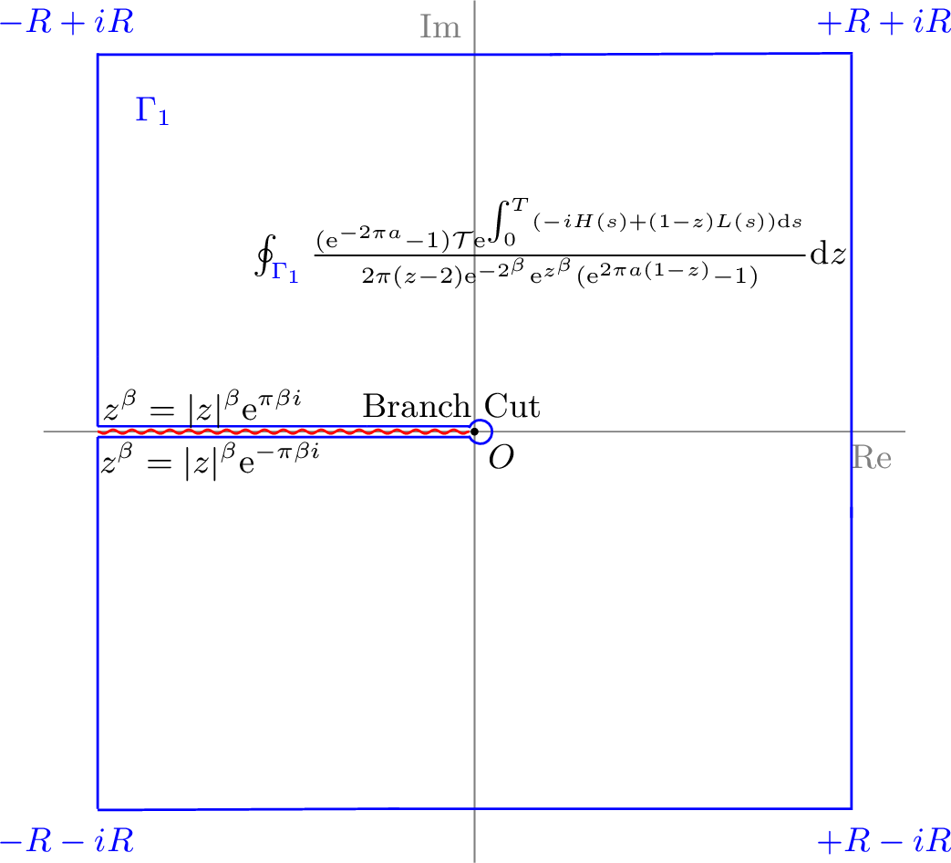
If \(\beta \in (0, 1)\) is a fixed real number, the integrand decays sub-exponentially on the large arcs of the contour. Simultaneously, when \(\| \int_{0}^{T}L(s) \mathrm{d}s\| \leq 2\pi a\), along the integration path from \(-\sqrt{R}\pm i R\) to \(+\sqrt{R}\pm i R\), term \(\frac{ \mathcal{T}\mathrm{e}^{\int_{0}^{T}(- i H(s)+(1-z)L(s))\mathrm{d}s} }{\mathrm{e}^{2\pi a(1-z)}-1 }\) can be bounded by a constant, while the remaining part tends to 0. According to Cauchy’s estimate, we get that the integral over the outer square contour tends to 0. The sum of the residues at the poles must be equal to the negative of the integral along the branch cut. This leads to the identity: \[\begin{align} \label{improved95int} &{ \mathcal{T}\mathrm{e}^{-\int_{0}^{T}A(s)\mathrm{d}s} }-\frac{1}{a}\sum_{k\in\mathbb{Z}}{\frac{ ({\mathrm{e}^{-2\pi a}-1}) \mathcal{T}\mathrm{e}^{- i \int_{0}^{T}H(s)+\frac{k}{a}L(s)\mathrm{d}s} }{2\pi i (k/a+ i )\mathrm{e}^{-2^{\beta}}\mathrm{e}^{( i k/a+1)^{\beta}} }}\\ =&\int_{0}^{+\infty}{\frac{ i ({\mathrm{e}^{-2\pi a}-1}) \mathcal{T}\mathrm{e}^{\int_{0}^{T}(- i H(s)+(1+z)L(s))\mathrm{d}s} }{\pi (z+2)\mathrm{e}^{-2^{\beta}}(\mathrm{e}^{2\pi a(1+z)}-1) }\mathrm{e}^{-z^{\beta}\cos(\pi\beta)}\sin(z^{\beta}\sin\pi\beta) \mathrm{d}z }. \end{align}\tag{18}\]
To control the error, we can rearrange Eq. 18 into the sum of \(\epsilon_{\text{IR}}\) and truncation error: \[\begin{align} \label{improved95err} &\left\|{ \mathcal{T}\mathrm{e}^{-\int_{0}^{T}A(s)\mathrm{d}s} }-\sum_{|k|\leq K}{\frac{ ({\mathrm{e}^{-2\pi a}-1}) \mathcal{T}\mathrm{e}^{- i \int_{0}^{T}H(s)+\frac{k}{a}L(s)\mathrm{d}s} }{2\pi i (k/a+ i )\mathrm{e}^{-2^{\beta}}\mathrm{e}^{( i k/a+1)^{\beta}} }}\right\|\\ \leq&\left\|\int_{0}^{+\infty}{\cdots}\mathrm{d}z\right\| +\left\|\sum_{|k|> K}{\frac{ ({\mathrm{e}^{-2\pi a}-1}) \mathcal{T}\mathrm{e}^{- i \int_{0}^{T}H(s)+\frac{k}{a}L(s)\mathrm{d}s} }{2\pi i (k/a+ i )\mathrm{e}^{-2^{\beta}}\mathrm{e}^{( i k/a+1)^{\beta}} }}\right\|\leq \epsilon. \end{align}\tag{19}\] We bound each term on the right-hand side. The \(\epsilon_{\text{IR}}\) can be bounded by \(\mathrm{e}^{\int_{0}^{T}\alpha_{\max}(t)\mathrm{d}t-2\pi a}\), the truncated series can be bounded by \(\epsilon/2\) by letting \(K/a\in \mathcal{O}((\log(1/\epsilon))^{1/\beta})\) [11].
Hence, we can set \(a=\| \int_{0}^{T}L(s) \mathrm{d}s\|+\log\frac{1}{\epsilon}\) and \[K= \mathcal{O} \left((\| \int_{0}^{T}L(s) \mathrm{d}s\|+\log\frac{1}{\epsilon})\left(\log\frac{1}{\epsilon}\right)^{1/\beta}\right)\] to satisfy the condition in Eq. 19 . Then, considering the norm scaling of the initial and final vectors and EST, the final number of coefficients is \(2K+1\), with \[\max_{j}|k'_{j}| = \mathcal{O}\left(\left(\log\frac{\|u_0\|}{\|u_{T}\|\epsilon}\right)^{1/\beta}\right).\] The number of queries to \(A(t)\) is \[\widetilde{\mathcal{O}}\left( \frac{\|u_0\|}{\|u_T\|} \alpha_{d} T\left(\log \frac{1}{\epsilon}\right)^{1+1/\beta}\right),\] and for the time-independent case, the complexity is \[\widetilde{\mathcal{O}}\left( \frac{\|u_0\|}{\|u_T\|} \alpha_{d} T\left(\log \frac{1}{\epsilon}\right)^{1/\beta}\right).\] The number of queries to the initial state \(u_{0}\) is \[\mathcal{O}\left( \frac{\|u_0\|}{\|u_T\|}\right),\] and the coefficient number for the LCU becomes \[\mathcal{O}\left(\left(\log\frac{\|u_0\|}{\|u_{T}\|\epsilon}\right)^{1/\beta}\left(\log\frac{\|u_0\|}{\|u_{T}\|\epsilon} + \rho_{L}\right)\right).\]
Finally, we consider the \(h_2(z)\) function defined by [32], \(h_2(z)=\frac{z- i }{-2 i }\mathrm{e}^{\frac{z^2+1}{4\gamma^2}-c(1- i z)}\) to adapt this method to the CBMD framework, by replace \(h_1(z)=1\) with \(h_1(z)=\mathrm{e}^{-2\pi i a z} - 1\), we consider the following integral: \[\label{eqs95optimal95lchs} \int_{\Gamma_{2}}{ \frac{({\mathrm{e}^{-2\pi a}-1})\mathcal{T}\mathrm{e}^{- i \int_{0}^{T}(H(s)+zL(s))\mathrm{d}s}}{2\pi i (z+ i )(\mathrm{e}^{-2\pi i az}-1)h_{2}(z)}\mathrm{d}z, }\tag{20}\]
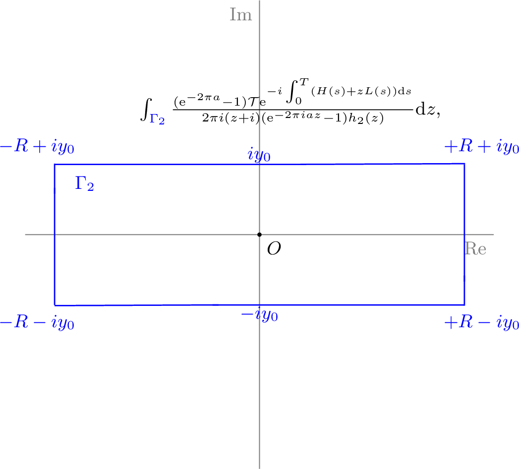
where \(\Gamma_2\) is a rectangular contour with vertices at \(- i y_{0}\pm R\) and \(i y_{0}\pm R\), as shown in Fig. 7. Here, \(y_{0}>1\) and we take the limit \(R\to\infty\) (e.g., by setting \(R=(2N+1)/(2a)\) for integer \(N\to\infty\)). Calculating the two vertical integrals, we find they vanish in the limit: \[\begin{align} &\Bigg{\|}\int_{- i y_{0}\pm R}^{ i y_{0}\pm R}{ \frac{({\mathrm{e}^{-2\pi a}-1})\mathcal{T}\mathrm{e}^{- i \int_{0}^{T}(H(s)+zL(s))\mathrm{d}s}}{2\pi i (z+ i )(\mathrm{e}^{-2\pi i az}-1)h_{2}(z)}\mathrm{d}z }\Bigg{\|}\\ \leq &\Bigg{\|}\int_{- i y_{0}\pm R}^{ i y_{0}\pm R}{ \frac{\mathcal{T}\mathrm{e}^{- i \int_{0}^{T}(H(s)+zL(s))\mathrm{d}s}}{\pi(z^2+1)(\mathrm{e}^{-2\pi i az}-1)}\mathrm{e}^{-\frac{z^2+1}{4\gamma^2}+c(1- i z)}\mathrm{d}z }\Bigg{\|}\\ =&\Bigg{\|} i y_{0}\int_{-1}^{1}{ \frac{\mathcal{T}\mathrm{e}^{\int_{0}^{T}(- i H(s)\mp i RL(s)+uy_{0}L(s))\mathrm{d}s}\mathrm{e}^{c(1+uy_0\mp i R)}}{\pi(R^2-u^2y_{0}^{2}\pm 2 i uy_{0}R+1)(\mathrm{e}^{2\pi auy_{0}\mp 2\pi i aR}-1)}\mathrm{e}^{-\frac{(R^2-u^2y_{0}^{2}\pm 2 i uy_{0}R+1)}{4\gamma^2}}\mathrm{d}u }\Bigg{\|}\\ \leq & y_{0}\int_{-1}^{1}{ \frac{\mathrm{e}^{-\frac{(R^2-u^2y_{0}^{2})}{4\gamma^2}}\mathrm{e}^{c(1+uy_0)}}{\pi(R^2-y_{0}^{2}+1)}\mathrm{d}u }\\ \in&\mathcal{O}(R^{-2})\to 0, \quad \text{as } R\to \infty. \end{align}\] This result matches the conclusion from the analysis in [32]. By CBMD, then we obtain the following identity: \[\begin{align} \label{Super95Eq123} &\mathcal{T}\mathrm{e}^{-\int_{0}^{T}A(s)\mathrm{d}s}- \frac{1-\mathrm{e}^{-2\pi a}}{a}\sum_{k\in \mathbb{Z}}{ \frac{\mathcal{T}\mathrm{e}^{- i \int_{0}^{T}(H(s)+(k/a)L(s))\mathrm{d}s}}{\pi((k/a)^2+1)}\mathrm{e}^{-\frac{(k/a)^2+1}{4\gamma^2}+c(1- i (k/a))} }\\ &-\frac{\mathrm{e}^{-2\pi a}-1}{\mathrm{e}^{2\pi a}-1}\mathrm{e}^{2c}\mathcal{T}\mathrm{e}^{\int_{0}^{T}- i H(s)+L(s)\mathrm{d}s} \\ =&\int_{- i y_{0}- R}^{- i y_{0} + R}{ \frac{(1-\mathrm{e}^{-2\pi a})\mathcal{T}\mathrm{e}^{- i \int_{0}^{T}(H(s)+zL(s))\mathrm{d}s}}{\pi(z^2+1)(\mathrm{e}^{-2\pi i az}-1)}\mathrm{e}^{-\frac{z^2+1}{4\gamma^2}+c(1- i z)}\mathrm{d}z }\\ &+\int_{ i y_{0}- R}^{ i y_{0} + R}{ \frac{(1-\mathrm{e}^{-2\pi a})\mathcal{T}\mathrm{e}^{- i \int_{0}^{T}(H(s)+zL(s))\mathrm{d}s}}{\pi(z^2+1)(\mathrm{e}^{-2\pi i az}-1)}\mathrm{e}^{-\frac{z^2+1}{4\gamma^2}+c(1- i z)}\mathrm{d}z}. \end{align}\tag{21}\] From Corollary 6 of Ref. [32], we take \(a \geq \| \int_{0}^{T}L(s) \mathrm{d}s\| + \log\frac{1}{\epsilon}+ 2c\), \(y_0=2c\gamma^2\), where \(L(s)\) is a semi-positive definite matrix. We can then estimate the integrals: \[\begin{align} \label{T1} \epsilon_{\text{IR}} = & \left\| \int_{- i y_{0}- R}^{- i y_{0} + R}{\cdots\mathrm{d}z} \right\| + \left\| \int_{ i y_{0}- R}^{ i y_{0} + R}{\cdots\mathrm{d}z} \right\|\\ \leq &\int_{- i y_{0}- R}^{- i y_{0} + R}{\left| \frac{\mathrm{e}^{-\frac{z^2+1}{4\gamma^2}+c(1- i z)}}{\pi(z^2+1)}\mathrm{e}^{-y_0\eta_{\min}}\right|\mathrm{d}z }+\int_{ i y_{0}- R}^{ i y_{0} + R}{\left| \frac{\mathrm{e}^{-\frac{z^2+1}{4\gamma^2}+c(1- i z)}}{\pi(z^2+1)}\frac{\mathrm{e}^{y_{0}\| \int_{0}^{T}L(s) \mathrm{d}s\|}}{\mathrm{e}^{-2\pi i az}-1} \right|\mathrm{d}z } \\ \leq & \mathrm{e}^{c-c^2\gamma^2} + \epsilon^{y_{0}}\mathrm{e}^{c+c^2\gamma^2}=\mathrm{e}^{c-c^2\gamma^2} + \epsilon^{2c\gamma^2}\mathrm{e}^{c+c^2\gamma^2}=\mathrm{e}^{c-c^2\gamma^2}(1+\epsilon^{2c\gamma^2}\mathrm{e}^{c+2c^2\gamma^2}), \end{align}\tag{22}\] here, \(c\) is a constant. If we take \(\gamma \in \mathcal{O}(\frac{1}{c}\sqrt{c+\log\frac{1}{\epsilon}})\), the bound \(\epsilon_{\text{IR}}\leq \epsilon/3\) holds. The second term, which we define as \(\epsilon_{\text{AE}}\), is bounded as follows: \[\begin{align} \epsilon_{\text{AE}}=& \Bigg{\|}-\frac{\mathrm{e}^{-2\pi a}-1}{\mathrm{e}^{2\pi a}-1}\mathrm{e}^{2c}\mathcal{T}\mathrm{e}^{\int_{0}^{T}- i H(s)+L(s)\mathrm{d}s}\Bigg{\|}\\ \leq& \frac{\mathrm{e}^{\| \int_{0}^{T}L(s) \mathrm{d}s\|+2c}}{\mathrm{e}^{2\pi a}-1}\leq \epsilon/3. \end{align}\] Finally, we consider the truncated error, and bound it by \(\epsilon/3\): \[\begin{align} &\Bigg{\|}\frac{1-\mathrm{e}^{-2\pi a}}{a}\sum_{|k|>K}{ \frac{\mathcal{T}\mathrm{e}^{- i \int_{0}^{T}(H(s)+(k/a)L(s))\mathrm{d}s}}{\pi((k/a)^2+1)}\mathrm{e}^{-\frac{(k/a)^2+1}{4\gamma^2}+c(1- i (k/a))} }\Bigg{\|}\\ \leq &2\sum_{k>K}{ \frac{\mathrm{e}^c}{a\pi((k/a)^2+1)}\mathrm{e}^{-\frac{(k/a)^2+1}{4\gamma^2}} }\leq \epsilon/3, \end{align}\] where the inequality holds if \(K/a \in\mathcal{O}(2c\gamma^2)\), \(\gamma\geq c^{-3/4}\), and \(\gamma=\frac{1}{c}\sqrt{c+\log\frac{1}{2\pi \epsilon}}\), as shown in Lemma 8 of [32]. Thus, our target approximation is satisfied: \[\begin{align} \label{Super95Eq2} &\left\|\mathcal{T}\mathrm{e}^{-\int_{0}^{T}{A(s)}\mathrm{d}s}-\frac{1-\mathrm{e}^{-2\pi a}}{a}\sum_{|k|\leq K}{ \frac{\mathcal{T}\mathrm{e}^{- i \int_{0}^{T}(H(s)+(k/a)L(s))\mathrm{d}s}}{\pi((k/a)^2+1)}\mathrm{e}^{-\frac{(k/a)^2+1}{4\gamma^2}+c(1- i (k/a))} }\right\|\\ \leq &\epsilon_{\text{IR}} + \epsilon_{\text{AE}} + \epsilon/3 \leq \epsilon. \end{align}\tag{23}\] Combining the analysis above, we find that \(K/a\in\mathcal{O}(\frac{1}{c}\log\frac{1}{\epsilon})\) and \(a \in\mathcal{O}( \| \int_{0}^{T}L(s) \mathrm{d}s\| + \log\frac{1}{\epsilon}+c)\). The sum of the absolute values of the coefficients is \(\mathcal{O}(\mathrm{e}^{c}\mathrm{erfc}(\frac{1}{2\gamma}))\), which determines the number of repetitions for amplitude amplification.
Then, considering the norm scaling of the initial and final vectors, the final number of coefficients is \(2K+1\), with \[\max_{j}|k'_{j}| \in \mathcal{O}\left(\frac{1}{c}\left(\log\frac{\|u_0\|}{\|u_{T}\|\epsilon}\right)\right).\] The number of queries to \(A(t)\) is \[\widetilde{\mathcal{O}}\left(\mathrm{e}^{c}\mathrm{erfc}\left(\frac{1}{2\gamma}\right) \frac{\|u_0\|}{c\|u_T\|} \alpha_{d} T\left(\log \frac{1}{\epsilon}\right)^{2}\right),\] and for the time-independent case, the complexity is \[\widetilde{\mathcal{O}}\left(\mathrm{e}^{c}\mathrm{erfc}\left(\frac{1}{2\gamma}\right) \frac{\|u_0\|}{c\|u_T\|} \alpha_{d} T\log \frac{1}{\epsilon}\right).\] The number of queries to \(u_{0}\) is \[\mathcal{O}\left(\mathrm{e}^{c}\mathrm{erfc}\left(\frac{1}{2\gamma}\right) \frac{\|u_0\|}{\|u_T\|}\right),\] and the coefficient number for the LCU becomes \[\mathcal{O}\left(\frac{1}{c}\left(\log\frac{\|u_0\|}{\|u_{T}\|\epsilon}\right)\left(\log\frac{\|u_0\|}{\|u_{T}\|\epsilon} + \rho_{L}+c\right)\right).\] We typically choose \(c\) to be a constant around 1. As \(\epsilon \to 0\), \(\gamma\) becomes large and \(\mathrm{erfc}(1/2\gamma) \to 1\). Therefore, the factors \(c\), \(\mathrm{e}^c\), and \(\mathrm{erfc}(1/2\gamma)\) can be treated as constants and omitted from the asymptotic complexity scaling. This yields the same complexity as our CBMD+EST method.
10 Proof of Non-Hermitian Wave Equation Theorem 2↩︎
The evolution of the state \(u(t)\) at an arbitrary time \(t > 0\) can be described by: \[\frac{d^2}{dt^2}u(t) = -A u(t), \quad u(0) = u_0, \quad \frac{d}{dt}u(0) = 0\] where \(A = L + iH\) is a general non-Hermitian operator, with \(L, H \in \mathbb{C}^{N \times N}\) being Hermitian matrices and \(L\succ 0, H\succ 0\). Analytical solution at time \(t\) is given by the matrix wave propagator: \[u(t) = \cos\left(\sqrt{A}t\right) u_0 = \cos\left(\sqrt{L + iH}t\right) u_0\] Since the Taylor expansion of the cosine function contains only even powers, the square root branch cuts vanish, making the operator \(\cos(\sqrt{A}t)\) an entire function globally well-defined on \(\mathbb{C}\). Our objective is to prepare a normalized quantum state \(|u(t)\rangle\) with a success probability of \(\Omega(1)\) and within a precision of \(\epsilon\).
To decompose the non-Hermitian function into an LCU composed of purely Hermitian arguments, we construct the following complex-valued auxiliary function parameterized by \(t\): \[F(z) = \frac{h(1) \cos\left(\sqrt{izH + L} \;t\right)}{h(z) \cdot z(z-1)}\] where \(h(z) = \cos\left(\sqrt{2\pi a i z} \;t\right)\).
Let \(\alpha_{\max}\) be the maximum spectral norm of \(H\). To suppress the asymptotic growth of the numerator (\(\sim \exp(t\sqrt{\alpha_{\max}|z|})\)), the scaling parameter \(a \in \mathbb{R}^+\) simply needs to satisfy \(2\pi a \geq \alpha_{\max}\), we can set \(2\pi a = \alpha_{\max}\) when \(\|H\|\) is known.
The function \(h(z)\) is an entire function, and its reciprocal yields strictly simple poles. By Cauchy’s Residue Theorem on a contour extending to infinity \(\sum \text{Res}(F, z_p) = 0\).
The target pole at \(z=1\) and origin pole at \(z=0\): \[\begin{align} \text{Res}(1) &= \lim_{z \to 1} (z-1)F(z) = \cos\left(\sqrt{A} \;t\right) \\ \text{Res}(0) &= \lim_{z \to 0} zF(z) = -h(1) \cos\left(\sqrt{L} \;t\right) \quad (\text{since } h(0) = 1) \end{align}\]
The infinite sequence of poles \(z_k\): The roots of \(\cos(w) = 0\) occur at \(w_k = (k+1/2)\pi\). Thus, the poles of \(h(z)\) satisfy \(\sqrt{2\pi a i z} t = (k+1/2)\pi\) for \(k \in \mathbb{Z}^{+}\cup \{0\}\). Solving for \(z\), all poles perfectly align on the negative imaginary axis: \[z_k = -i \frac{(k + 1/2)^2 \pi}{2a t^2}, \quad k = 0, 1, 2, \dots\] We compute the derivative \(h'(z)\) evaluated at \(z_k\). Let \(w = \sqrt{2\pi a i z}t\), yielding \(\frac{dw}{dz} = \frac{\pi a i t^2}{w}\). \[h'(z_k) = \left. \left( -\sin(w) \frac{\pi a i t^2}{w} \right) \right|_{w=(k+1/2)\pi} = (-1)^{k+1} \frac{a i t^2}{k+1/2}\] Evaluating the polynomial part of the denominator at \(z_k\): \[\begin{align} h'(z_k) z_k (z_k - 1) = &(-1)^{k+1} \frac{a i t^2}{k+1/2} \left( -i \frac{(k+1/2)^2 \pi}{2a t^2} \right) (z_k - 1) \\ =& (-1)^k \frac{(k+1/2)\pi}{2} \left( 1 + i\frac{(k+1/2)^2\pi}{2a t^2} \right) \end{align}\] The numerator at \(z_k\) undergoes the Hermitian reversal: \(iz_k H + L = \frac{(k+1/2)^2\pi}{2a t^2}H + L\).
Isolating \(\text{Res}(1)\), we obtain the exact LCU identity: \[\begin{align} \cos\left(\sqrt{A}t\right) = & \underbrace{h(1) \cos\left(\sqrt{L}t\right) - h(1) \sum_{k=0}^K d_k \cos\left(\sqrt{\frac{(k+1/2)^2\pi}{2a t^2}H + L} \;t\right)}_{\text{Quantum Circuit Implementation by QSVT+LCU}} \\& - \underbrace{h(1) \sum_{k=K+1}^\infty d_k \cos\left(\sqrt{\frac{(k+1/2)^2\pi}{2a t^2}H + L} \;t\right)}_{\text{Truncation Error}}, \end{align}\] where the coefficients are given by: \[d_k = \frac{(-1)^k}{\frac{(k+1/2)\pi}{2} \left( 1 + i \frac{(k+1/2)^2\pi}{2a t^2} \right)}.\] To estimate the infinite sum \(\sum_{k=1}^{\infty} |d_k|\) in the asymptotic regime of large \(at^2\), we first evaluate the magnitude of the terms, yielding \(|d_k| = \frac{2}{\pi(k+1/2)}\left[1 + \frac{\pi^2(k+1/2)^4}{4a^2t^4}\right]^{-1/2}\). By approximating the discrete summation with a continuous integral over \(k\), we observe that the integrand exhibits two distinct asymptotic behaviors separated by a crossover scale \(k_c \sim \sqrt{at}\). In the regime where \(k \ll k_c\), the higher-order term inside the square root is negligible, reducing the summand to \(\mathcal{O}(k^{-1})\), whereas for \(k \gg k_c\), the summand rapidly decays as \(\mathcal{O}(k^{-3})\), ensuring absolute convergence. The principal contribution to the total sum arises from the slowly decaying lower domain \([1, k_c]\), which yields a logarithmic accumulation \(\int_1^{\sqrt{at}} k^{-1} \,dk \sim \ln(\sqrt{at})\). Consequently, for a sufficiently large parameter \(at^2\), the final estimation of the summation scales asymptotically as \[\label{eq:estmdk} \sum_{k=1}^{\infty} |d_k|\sim \mathcal{O}(\log(at)).\tag{24}\]
Here we need bounded the truncation error by \(\epsilon'\), we get: \[\begin{align} &h(1) \sum_{k=K+1}^\infty d_k \cos\left(\sqrt{\frac{(k+1/2)^2\pi}{2a t^2}H + L} \;t\right)\\ \leq&h(1) \sum_{k=K+1}^\infty \frac{1}{\frac{(k+1/2)\pi}{2} \frac{(k+1/2)^2\pi}{2a t^2} }\leq\epsilon'/2, \end{align}\]here we can set \(K\sim \mathcal{O}(\frac{\sqrt{a}t}{\sqrt{\epsilon'/h(1)}})\) to get the truncation errer bounded by \(\epsilon'/2\).
As for the success probility from LCU, we need consider the 1-norm of the coefficients \(h(1)(1 + \sum_{k=0}^\infty |d_k|)\sim \mathcal{O}(h(1)\log(at^2))\) by Eq. 24 . Consequently, the amplitude amplification factor is on the order of \(\mathcal{O}\left(\frac{h(1)\log(at^2)}{\|\cos(\sqrt{A}t)|\psi_0 \rangle\|}\right)\).
We define the \(k\)-th purely Hermitian operator as \(M_k = \frac{(k+1/2)^2\pi}{2a t^2}H + L\). To implement the operator \(\cos(\sqrt{M_k}t)\) via QSVT, we consider the time-scaled operator \(M_k t^2\). Its spectral norm is rigorously bounded by: \[\Lambda_K = \|M_k t^2\| \le \frac{(K+1/2)^2\pi}{2a}\alpha_{\max} + \alpha_{\max}(L)t^2 = \mathcal{O}(K^2 + \alpha_{\max}(L)t^2)\]
To satisfy the global boundedness requirement of QSVT on the entire domain \([-1, 1]\), we cannot simply use the Taylor series truncation. Instead, we must apply QSVT polynomial patching to suppress the exponential divergence of \(\cos(\sqrt{\Lambda_K x})\) on the non-physical negative real axis. This patching cost scales with the inverse spectral gap of the system, which is strictly bounded by the condition number \(\kappa = \max(\kappa_H, \kappa_L)\) assuming strictly positive definite \(H\) and \(L\). To achieve precision \(\epsilon_{\text{qsvt}}\) (where \(h(1)at^2\epsilon_{\text{qsvt}}\leq\epsilon'/2\), meaning \(\epsilon_{\text{qsvt}}\sim \mathcal{O}(\frac{\epsilon'}{h(1)a t^2})\)), and regarding \(\alpha_{\max}(L)\) as a constant, the estimation of \(D_K\) is: \[D_K= \mathcal{O}\left( \kappa \left[ K + \sqrt{\alpha_{\max}(L)}t + \log\left(\frac{1}{\epsilon_{\text{qsvt}}}\right) \right] \right)=\mathcal{O}\left( \kappa \frac{\sqrt{ah(1)}t}{\sqrt{\epsilon'}} \right).\]
Finally we replace the \(\epsilon'\) by \(\|\cos(\sqrt{A}t)|\psi_0 \rangle\| \epsilon\) and combine the times of amplitude amplification factor we get the total query to matrix \(A\) is: \[\tilde{\mathcal{O}}\left(\kappa \frac{h(1)\log(at^2)}{\|\cos(\sqrt{A}t)|\psi_0 \rangle\|} \sqrt{\frac{ah(1)}{\|\cos(\sqrt{A}t)|\psi_0 \rangle\|\epsilon} } t \right).\]
and the query to state preparation of \(|u_0\rangle\) is about: \[{\mathcal{O}}\left( \frac{h(1)\log(at^2)}{\|\cos(\sqrt{A}t)|\psi_0 \rangle\|} \right),\] here \(h(1)\) scales about \(h(1)\sim \frac{e^{\sqrt{\pi a}t}}{2}\).
11 Proof of Non-Hermitian Bessel Equation Theorem 3↩︎
The evolution of the state \(u(t)\) at an arbitrary time \(t > 0\) can be described by: \[\frac{d^2u(t)}{dt^2} + \frac{1}{t} \frac{du(t)}{dt} + A u(t) = 0,\] where \(A = L + iH\) is a general non-Hermitian operator, with \(L, H \in \mathbb{C}^{N \times N}\) being Hermitian matrices and \(L\succ 0, H\succ 0\). Analytical solution at time \(t\) is given by the matrix Bessel function: \[u(t) = J_{0}\left(\sqrt{A}t\right) u_0 = J_{0}\left(\sqrt{L + iH}t\right) u_0\] Since the Taylor expansion of the cosine function contains only even powers, the square root branch cuts vanish, making the operator \(J_{0}(\sqrt{ i zH+L}t)\) an entire function globally well-defined on \(\mathbb{C}\). Our objective is to prepare a normalized quantum state \(|u(t)\rangle\) with a success probability of \(\Omega(1)\) and within a precision of \(\epsilon\).
To decompose the non-Hermitian function into an LCU composed of purely Hermitian arguments, we construct the following complex-valued auxiliary function parameterized by \(t\): \[F(z) = \frac{h(1) J_0(\sqrt{ i zH+L}t)}{h(z) z(z-1)},\] where \(h(z) = \cos\left(\sqrt{2\pi a i z} \;t\right)\).
Let \(\alpha_{\max}\) be the maximum spectral norm of \(H\). To suppress the asymptotic growth of the numerator (\(\sim \exp(t\sqrt{\alpha_{\max}|z|})\)), the scaling parameter \(a \in \mathbb{R}^+\) simply needs to satisfy \(2\pi a \geq \alpha_{\max}\), we can set \(2\pi a = \alpha_{\max}\) when \(\|H\|\) is known.
To rigorously establish that the contour integral of \(F(z)\) vanishes over a sequence of expanding circular contours at infinity, we examine its asymptotic behavior as \(|z| \to \infty\). The numerator involves the Bessel function \(J_0(\sqrt{ i zH+L}t)\), which is an entire function of order \(1/2\). Its maximum asymptotic growth in the complex plane is governed by \(\exp(c\sqrt{|z|\|H\|})\), where the matrix norm \(\|H\| = 2\pi a\) defines the maximum exponential type. Provided that the characteristic function \(h(z)\) in the denominator exhibits a compatible growth rate that asymptotically bounds the numerator, the ratio \(h(1)J_0(\sqrt{ i zH+L}t)/h(z)\) remains uniformly bounded on a sequence of carefully chosen contours \(\Gamma\) with radii \(R \to \infty\). Consequently, the overall integrand is strictly dominated by the rational term \(1/(z(z-1))\), yielding an asymptotic decay of \(F(z) = \mathcal{O}(R^{-2})\). By the estimation lemma (ML inequality), the norm of the integral is bounded by \(\mathcal{O}(R^{-1})\), which rigorously vanishes in the limit of infinite radius. The function \(h(z)\) is an entire function, and its reciprocal yields strictly simple poles. By Cauchy’s residue theorem on a contour extending to infinity, \(\sum \text{Res}(F, z_p) = 0\).
The target pole at \(z=1\) and origin pole at \(z=0\): \[\begin{align} \text{Res}(1) &= \lim_{z \to 1} (z-1)F(z) = J_{0}\left(\sqrt{A} \;t\right) \\ \text{Res}(0) &= \lim_{z \to 0} zF(z) = -h(1) J_{0}\left(\sqrt{L} \;t\right) \quad (\text{since } h(0) = 1) \end{align}\]
The infinite sequence of poles \(z_k\): \[\begin{align} h'(z_k) z_k (z_k - 1) = &(-1)^{k+1} \frac{a i t^2}{k+1/2} \left( - i \frac{(k+1/2)^2 \pi}{2a t^2} \right) (z_k - 1) \\ =& (-1)^k \frac{(k+1/2)\pi}{2} \left( 1 + i \frac{(k+1/2)^2\pi}{2a t^2} \right) \end{align}\] The numerator at \(z_k\) undergoes the Hermitian reversal: \(i z_k H + L = \frac{(k+1/2)^2\pi}{2a t^2}H + L\).
Isolating \(\text{Res}(1)\), we obtain the exact LCU identity: \[\begin{align} J_{0}\left(\sqrt{A}t\right) = & \underbrace{h(1) J_{0}\left(\sqrt{L}t\right) + h(1) \sum_{k=0}^K d_k J_{0}\left(\sqrt{\frac{(k+1/2)^2\pi}{2a t^2}H + L} \;t\right)}_{\text{Quantum Circuit Implementation by QSVT+LCU}} \\& + \underbrace{h(1) \sum_{k=K+1}^\infty d_k J_{0}\left(\sqrt{\frac{(k+1/2)^2\pi}{2a t^2}H + L} \;t\right)}_{\text{Truncation Error}} \end{align}\] where the coefficients are given by: \[d_k = \frac{(-1)^k}{\frac{(k+1/2)\pi}{2} \left( 1 + i \frac{(k+1/2)^2\pi}{2a t^2} \right)}\]
Here we need bounded the truncation error by \(\epsilon'\), we get: \[\begin{align} &h(1) \sum_{k=K+1}^\infty d_k J_{0}\left(\sqrt{\frac{(k+1/2)^2\pi}{2a t^2}H + L} \;t\right)\\ \leq&h(1) \sum_{k=K+1}^\infty \frac{1}{\frac{(k+1/2)\pi}{2} \frac{(k+1/2)^2\pi}{2a t^2} }\leq\epsilon'/2, \end{align}\]here we can set \(K\sim \mathcal{O}(\frac{\sqrt{a}t}{\sqrt{\epsilon'/h(1)}})\) to get the truncation errer bounded by \(\epsilon'/2\).
As for the success probility from LCU, we need consider the 1-norm of the coefficients \(h(1)(1 + \sum_{k=0}^\infty |d_k|)\sim \mathcal{O}(h(1)\log(at^2))\) by Eq. 24 . Consequently, the amplitude amplification factor is on the order of \(\mathcal{O}\left(\frac{h(1)\log(at^2)}{\|J_{0}(\sqrt{A}t)|\psi_0 \rangle\|}\right)\).
We define the \(k\)-th purely Hermitian operator as \(M_k = \frac{(k+1/2)^2\pi}{2a t^2}H + L\). To implement the operator \(J_{0}(\sqrt{M_k}t)\) via QSVT, we consider the time-scaled operator \(M_k t^2\). Its spectral norm is rigorously bounded by: \[\Lambda_K = \|M_k t^2\| \le \frac{(K+1/2)^2\pi}{2a}\alpha_{\max} + \alpha_{\max}(L)t^2 = \mathcal{O}(K^2 + \alpha_{\max}(L)t^2)\]
To satisfy the global boundedness requirement of QSVT, we cannot simply use the Taylor series truncation. Instead, we must apply QSVT polynomial patching to suppress the exponential divergence of the modified Bessel function \(I_0(\sqrt{\Lambda_K |x|})\) on the non-physical negative real axis. This patching cost scales with the inverse spectral gap, which is strictly bounded by the condition number \(\kappa = \max(\kappa_H, \kappa_L)\) assuming strictly positive definite \(H\) and \(L\). To achieve precision \(\epsilon_{\text{qsvt}}\) (where \(h(1)at^2\epsilon_{\text{qsvt}}\leq\epsilon'/2\), meaning \(\epsilon_{\text{qsvt}}\sim \mathcal{O}(\frac{\epsilon'}{h(1)a t^2})\)), and regarding \(\alpha_{\max}(L)\) as a constant, the estimation of \(D_K\) is: \[D_K= \mathcal{O}\left( \kappa \left[ K + \sqrt{\alpha_{\max}(L)}t + \log\left(\frac{1}{\epsilon_{\text{qsvt}}}\right) \right] \right)=\mathcal{O}\left( \kappa \frac{\sqrt{ah(1)}t}{\sqrt{\epsilon'}} \right).\]
Finally we replace the \(\epsilon'\) by \(\|J_{0}(\sqrt{A}t)|\psi_0 \rangle\| \epsilon\) and combine the times of amplitude amplification factor we get the total query to matrix \(A\) is: \[\tilde{\mathcal{O}}\left( \kappa\frac{h(1)\log(at^2)}{\|J_{0}(\sqrt{A}t)|\psi_0 \rangle\|} \sqrt{\frac{ah(1)}{\|J_{0}(\sqrt{A}t)|\psi_0 \rangle\|\epsilon} } t \right).\]
and the query to state preparation of \(|u_0\rangle\) is about: \[{\mathcal{O}}\left( \frac{h(1)\log(at^2)}{\|J_{0}(\sqrt{A}t)|\psi_0 \rangle\|} \right),\] here \(h(1)\) scales about \(h(1)\sim \frac{e^{\sqrt{\pi a}t}}{2}\).
From the above discussion, it can be seen that, apart from being a bit more careful when estimating the order of decay of the function at infinity, all the analysis is almost no different from that in the wavefunction case; the same is true when performing truncation using QSVT.
12 Proof of Non-Hermitian Airy Dynamics Theorem 4↩︎
The evolution of the state \(u(t)\) at an arbitrary time \(t > 0\) can be described by the matrix Airy differential equation: \[\frac{d^2u(t)}{dt^2} + t A u(t) = 0,\] where \(A = L + i H\) is a general non-Hermitian operator, with \(L, H \in \mathbb{C}^{N \times N}\) being Hermitian matrices and \(L\succ 0, H\succ 0\). The analytical solution at time \(t\) is given by the matrix function \(f(A^{1/3}t)u_{0}\), where the projected zero-velocity propagator is \[f(z) = \frac{1}{3} \left( \mathrm{Ai}(-z) + \mathrm{Ai}(-\omega z) + \mathrm{Ai}(-\omega^2 z) \right),\] and \(\omega = e^{2\pi i /3}\). Since the \(\mathbb{Z}_3\) root-of-unity projection strictly filters out all non-integer powers, the fractional roots perfectly annihilate, making the operator \(f(( i zH+L)^{1/3}t)\) an entire function globally well-defined on \(\mathbb{C}\) and completely free of branch cuts. Our objective is to prepare a normalized quantum state \(|u(t)\rangle\) with a success probability of \(\Omega(1)\) and within a precision of \(\epsilon\).
To decompose the non-Hermitian function into an LCU composed of purely Hermitian arguments, we construct the following complex-valued auxiliary function parameterized by \(t\): \[F(z) = \frac{h(1) f(( i zH+L)^{1/3}t)}{h(z) z(z-1)},\] where the tight-bound trigonometric regulator is chosen as \(h(z) = \cos\left(\frac{2}{3} t^{3/2} \sqrt{ i \gamma z}\right)\).
Let \(\alpha_{\max}\) be the maximum spectral norm of \(H\). To suppress the asymptotic growth of the numerator (\(\sim \exp(\frac{2}{3}t^{3/2}\sqrt{\alpha_{\max}|z|})\)), the bounding parameter \(\gamma \in \mathbb{R}^+\) simply needs to satisfy \(\gamma \geq \alpha_{\max}\). We can naturally set \(\gamma = \alpha_{\max} = \|H\|\) when \(\|H\|\) is known.
To rigorously establish that the contour integral of \(F(z)\) vanishes over a sequence of expanding circular contours at infinity, we examine its asymptotic behavior as \(|z| \to \infty\). The numerator involves the \(\mathbb{Z}_3\)-Airy function \(f(( i zH+L)^{1/3}t)\), which natively belongs to the \(\mathbb{Z}_3\) root-of-unity projection class of entire functions of order \(1/2\). Its maximum asymptotic growth in the complex plane is strictly governed by the envelope \(\exp(\frac{2}{3}\sqrt{|z|\|H\|t^3})\). Provided that the regulator \(h(z)\) in the denominator is configured with the tight matching rate \(\gamma \ge \|H\|\) to asymptotically bound the numerator, the ratio \(h(1)f(( i zH+L)^{1/3}t)/h(z)\) remains uniformly bounded on a sequence of carefully chosen contours \(\Gamma\) with radii \(R \to \infty\). Consequently, the overall integrand is strictly dominated by the rational term \(1/(z(z-1))\), yielding an asymptotic decay of \(F(z) = \mathcal{O}(R^{-2})\). By the estimation lemma (ML inequality), the norm of the integral is bounded by \(\mathcal{O}(R^{-1})\), which rigorously vanishes in the limit of infinite radius. The function \(h(z)\) is an entire function, and its reciprocal yields strictly simple poles. By Cauchy’s residue theorem on a contour extending to infinity, \(\sum \text{Res}(F, z_p) = 0\).
The target pole at \(z=1\) and origin pole at \(z=0\): \[\begin{align} \text{Res}(1) &= \lim_{z \to 1} (z-1)F(z) = f\left(A^{1/3} t\right) \\ \text{Res}(0) &= \lim_{z \to 0} zF(z) = -h(1) f\left(L^{1/3} t\right) \quad (\text{since } h(0) = \cos(0) = 1) \end{align}\]
The infinite sequence of poles \(z_k\) corresponds to the roots of the cosine function. By setting \(\frac{2}{3}t^{3/2}\sqrt{ i \gamma z_k} = (k+1/2)\pi\), we obtain \(z_k = - i \frac{9(k+1/2)^2\pi^2}{4\gamma t^3}\). The derivative evaluation yields: \[\begin{align} h'(z_k) z_k (z_k - 1) &= (-1)^{k+1} \frac{(k+1/2)\pi}{2} (z_k - 1) \\ &= (-1)^k \frac{(k+1/2)\pi}{2} \left( 1 + i \frac{9(k+1/2)^2\pi^2}{4\gamma t^3} \right) \end{align}\] The numerator at \(z_k\) undergoes the exact Hermitian reversal: \(i z_k H + L = \frac{9(k+1/2)^2\pi^2}{4\gamma t^3}H + L\).
Isolating \(\text{Res}(1)\), we obtain the exact LCU identity: \[\begin{align} f\left(A^{1/3}t\right) = & \underbrace{h(1) f\left(L^{1/3}t\right) + h(1) \sum_{k=0}^K d_k f\left(\left(\frac{9(k+1/2)^2\pi^2}{4\gamma t^3}H + L\right)^{1/3} t\right)}_{\text{Quantum Circuit Implementation by QSVT+LCU}} \\& + \underbrace{h(1) \sum_{k=K+1}^\infty d_k f\left(\left(\frac{9(k+1/2)^2\pi^2}{4\gamma t^3}H + L\right)^{1/3} t\right)}_{\text{Truncation Error}} \end{align}\] where the expansion coefficients are given by: \[d_k = \frac{(-1)^k}{\frac{(k+1/2)\pi}{2} \left( 1 + i \frac{9(k+1/2)^2\pi^2}{4\gamma t^3} \right)}\]
Here we need to bound the truncation error by \(\epsilon'\). Leveraging the uniform bound \(\|f(x)\| \le f(0) = \mathcal{O}(1)\) for all \(x \ge 0\), we get: \[\begin{align} & \left\| h(1) \sum_{k=K+1}^\infty d_k f\left(\left(\frac{9(k+1/2)^2\pi^2}{4\gamma t^3}H + L\right)^{1/3} t\right) \right\| \\ \leq& h(1) \sum_{k=K+1}^\infty \frac{1}{\frac{(k+1/2)\pi}{2} \frac{9(k+1/2)^2\pi^2}{4\gamma t^3} } \leq \epsilon'/2, \end{align}\] from which we can set \(K\sim \mathcal{O}\left(\frac{\sqrt{\gamma}t^{3/2}}{\sqrt{\epsilon'/h(1)}}\right)\) to get the truncation error bounded by \(\epsilon'/2\).
As for the success probability from LCU, we consider the \(1\)-norm of the coefficients \(h(1)(1 + \sum_{k=0}^\infty |d_k|) \sim \mathcal{O}(h(1)\log(\gamma t^3))\) nearly same as Eq. 24 . Consequently, the amplitude amplification factor is on the order of \(\mathcal{O}\left(\frac{h(1)\log(\gamma t^3)}{\|f(A^{1/3}t)|u_0 \rangle\|}\right)\).
We define the \(k\)-th purely Hermitian operator as \(M_k = \frac{9(k+1/2)^2\pi^2}{4\gamma t^3}H + L\). To implement the operator \(f(M_k^{1/3}t)\) via QSVT, the accumulated effective phase dictates the necessary polynomial degree. The spectral norm of \(M_k\) is rigorously bounded by: \[\|M_k\| \le \frac{9(K+1/2)^2\pi^2}{4\gamma t^3}\alpha_{\max} + \alpha_{\max}(L) = \mathcal{O}\left( \frac{K^2}{t^3} + \alpha_{\max}(L) \right)\]
To satisfy the global boundedness requirement of QSVT, we cannot simply apply the target polynomial approximation for the \(1/2\)-order function \(f(x)\). Instead, we must apply QSVT polynomial patching to suppress its exponential divergence on the non-physical negative real axis. This patching cost scales with the inverse spectral gap, which is strictly bounded by the condition number \(\kappa = \max(\kappa_H, \kappa_L)\) assuming strictly positive definite \(H\) and \(L\). The required polynomial degree \(D_K\) is bounded by the maximum asymptotic phase \(\mathcal{O}(\sqrt{\|M_k\|}t^{3/2})\) scaled by \(\kappa\) to achieve precision \(\epsilon_{\text{qsvt}}\). The error from QSVT should satisfy \(h(1) \epsilon_{\text{qsvt}} \leq \epsilon'/2\), which implies \(\epsilon_{\text{qsvt}} \sim \mathcal{O}(\frac{\epsilon'}{h(1)})\). Regarding \(\alpha_{\max}(L)\) as a constant, we have the estimation of \(D_K\): \[\begin{align} D_K=& \mathcal{O}\left( \kappa \left[ \sqrt{|M_k|}t^{3/2} + \log\left(\frac{1}{\epsilon_{\text{qsvt}}}\right) \right] \right)\;\\=& \mathcal{O}\left( \kappa \left[ K + \sqrt{\alpha_{\max}(L)}t^{3/2} + \log\left(\frac{h(1)}{\epsilon'}\right) \right] \right) = \mathcal{O}\left(\kappa \frac{\sqrt{\gamma h(1)}t^{3/2}}{\sqrt{\epsilon'}} \right). \end{align}\]
Finally, we replace \(\epsilon'\) by \(\|f(A^{1/3}t)|u_0 \rangle\| \epsilon\) and combine it with the required amplitude amplification factor to obtain the total query complexity to matrix \(A\): \[\tilde{\mathcal{O}}\left( \kappa\frac{h(1)\log(\gamma t^3)}{\|f(A^{1/3}t)|u_0 \rangle\|} \sqrt{\frac{\gamma h(1)}{\|f(A^{1/3}t)|u_0 \rangle\|\epsilon} } t^{3/2} \right).\]
And the query complexity to the state preparation oracle of \(|u_0\rangle\) is approximately: \[{\mathcal{O}}\left( \frac{h(1)\log(\gamma t^3)}{\|f(A^{1/3}t)|u_0 \rangle\|} \right),\] where the global exponential regulator scales as \(h(1) \sim \exp\left(\frac{2}{3} \sqrt{\gamma} t^{3/2}\right)\).