Keywords: Nonlinear systems, signatures, bilinear approximations, model order reduction, non-Lipschitz vector fields

MSC classification: 60L10, 65C30, 93A15, 93C10

1 Introduction↩︎

The study of nonlinear systems is motivated by their ability to represent complex real-world processes that linear models cannot adequately capture. In many cases, the underlying nonlinear model is unknown and only data are available, prompting the use of data-driven approaches to infer system behavior directly from observations. Moreover, when such systems are high-dimensional, their analysis becomes computationally demanding, motivating the development of reduced-order and data-efficient methods to capture essential dynamics. This paper proposes an approach to address the challenges discussed above. We develop a universal model capable of capturing the behavior of general nonlinear systems, while its unknown components can be inferred directly from observational data. The universal model can be high-dimensional, and we employ model order reduction (MOR) techniques to optimize it efficiently. Notably, high-dimensional nonlinear systems can often be accurately approximated by low-order bilinear systems using our approach, highlighting its potential for effective complexity reduction.

1.1 Existing results and comparison to the signature approach↩︎

This work lies at the interface of multiple disciplines. In particular, we exploit techniques from rough paths theory, MOR, and data-driven learning to establish connections between nonlinear and bilinear systems.

Path signatures play a crucial role in the theory of rough paths [1]–[3], which provides a deterministic integration framework for highly irregular paths, extending well beyond classical concepts such as Stieltjes and Young integration. For instance, it enables the pathwise definition of integrals with respect to fractional Brownian motion. Signatures also possess a universal approximation property [4], [5], enabling the learning of solutions to rough or stochastic differential equations. Beyond this, they have found compelling applications in fields such as finance [4], [6] and machine learning [7], demonstrating the versatility and power of signature-based approximations. This paper presents the concept of signatures within the context of control theory, with the goal of making them accessible without extensive background in algebra or rough paths, and demonstrates their application in learning nonlinear control systems. Specifically, we show that the output of a very general nonlinear system can be approximated by a linear map of a signature, which is a solution of a bilinear system that is unstable and has a non-zero initial state. The universality of bilinear systems is known in the control community, for example, see [8], [9] for existence results. Moreover, the Carleman linearization method [10], [11] highlights this perspective by using Taylor expansions of the system’s vector fields. However, the Carleman linearization requires certain regularity of the vector fields and typically ensures a small approximation error only locally. This is also true for the bilinearization proposed in [8]. Another limitation of Carleman’s method is that the dimension of the resulting bilinear system grows exponentially with the state dimension, making it impractical for large-scale systems. In contrast, our approach constructs a signature-based universal bilinear system that does not require smoothness of the underlying vector fields and is not limited to small neighborhoods for an accurate approximation. A key advantage is its applicability to high-dimensional systems, as the signature model grows only with the number of inputs. Finally, the computation of the signature model requires no knowledge of the underlying nonlinear system itself, relying solely on observational data of the system dynamics. It is perhaps unsurprising that the fundamental result underlying the universality of signatures is the Stone–Weierstrass theorem. This theorem has previously been applied to represent or approximate control systems [12]. However, that work employs these arguments to derive series representations of nonlinear systems in the sense of Volterra or Wiener, whereas our approach focuses on bilinearization.

Since signature models can be applied in high-dimensional settings, they are of particular interest in the context of MOR for nonlinear systems. Applying signature-based bilinearization to the original system results in a large-scale bilinear system. MOR for such systems has been extensively studied, with balanced truncation (BT) analyzed, for instance, in [13], [14]. BT offers the advantage of providing a comprehensive error analysis in the bilinear case [15]–[17]. However, existing approaches generally rely on asymptotic stability and zero initial states. Extensions to general initial conditions have been considered in [18], [19], but these methods still assume stability. In contrast, the signature-based bilinear system is neither stable nor initialized at zero. To address this, we study a time-limited version of BT specifically tailored to signature systems. Here, we propose Gramians and show their relations to dominant subspaces which is the fundament of the subsequent MOR procedure. Other MOR techniques, such as Krylov subspace-based or \(\mathcal{H}_2\)-optimal methods [20]–[23], cannot be directly applied in this setting, but they can be adapted to handle the lack of stability and nonzero initial conditions inherent to signature models.

Instead of relying on the bilinearization techniques proposed in this paper, MOR can be applied directly to nonlinear systems. Methods such as BT have been extended to nonlinear settings [24]–[26]. Related approaches that allow for the derivation of error bounds are also available [27], [28]. However, computing the system Gramians remains highly challenging for these methods, an issue we avoid by exploiting signature approximations. Projection-based MOR techniques have also been explored by transforming nonlinear dynamics into a quadratic-bilinear form via lifting [29]–[32]. Nevertheless, the analysis and computation of quadratic systems are significantly more involved than in the bilinear case. Data-driven MOR approaches [32]–[35] have been proved effective in addressing the challenge of identifying dominant subspaces in nonlinear systems. However, some of these methods require full access to the system’s governing equations, which is often impractical. Operator inference methods [36]–[40] can construct reduced-order models directly from data without explicit knowledge of the system coefficients. Yet, these approaches still require the underlying model structure to be known. This contrasts with our signature-based framework, which does not assume any prior knowledge of the system dynamics.

1.2 Framework and story in a nutshell↩︎

We study the following controlled differential equation endowed with the quality of interest \(y\): \[\tag{1} \begin{align} \tag{2} \dot{x}(t)&=f_0(x(t))+f(x(t))u(t),\quad x(0)=x_0,\\ \tag{3} y(t)&=c(x(t)), \end{align}\] where \(x:[0,T] \to \mathbb{R}^d\), \(u:[0,T]\to \mathbb{R}^m\), \(f_0:\mathbb{R}^d \to \mathbb{R}^d\), \(f:\mathbb{R}^d \to \mathbb{R}^{d\times m}\), \(y\colon[0,T] \to \mathbb{R}^{p}\) and \(c\colon \mathbb{R}^d\to \mathbb{R}^{p}\). Moreover, let \(f_0\), \(f\) and \(c\) be a locally Lipschitz continuous functions meaning, e.g., that for every \(R>0\) there is a constant \(L_{c, R}>0\) such that \(\|c(x)-c(z)\| \leq L_{c, R}\|x-z\|\) for all \(x\) and \(z\) with \(\|x\|, \|z\|\leq R\). We further assume that the control usually satisfies \(u\in L^2([0,T]; \mathbb{R}^m)\), but some considerations only require \(u\in L^1([0,T]; \mathbb{R}^m)\). Moreover, we suppose that 2 always has a unique global solution and will be more specific on the assumptions on \(f_0\) and \(f\) in Section 3 to ensure this.

In this work, we find a matrix \(C\in \mathbb{R}^{p\times n}\) such that \(y(\cdot)\approx CS(\cdot)\) in some sense, where \(S\) is the so-called truncated signature of \(\hat{U}(t) = (t, \int_0^t u(s)^\top\mathrm{d}s)^\top\), \(t\in[0, T]\), taking values in \(\mathbb{R}^n\). The computation of \(C\) does not require the knowledge of the nonlinear system, but only data of 1 . The truncated signature \(S\) satisfies a differential equation of the following form \[\begin{align} \label{tr95sig95ode} \dot{S}(t)=A_0 S(t) + \sum_{i=1}^{m} A_iS(t)u_i(t),\quad S(0)=s_0,\quad y_S(t)={C}S(t)\approx y(t), \end{align}\tag{4}\] where \(s_0\in\mathbb{R}^n\) is a particular fixed initial state, \(A_0, \dots, A_m\in \mathbb{R}^{n\times n}\) and \(u_1,\ldots,u_m\colon[0,T] \to \mathbb{R}\) are the components of \(u\). Usually, the dimension \(n\) is large. Therefore, dimension reduction techniques are designed, analyzed and applied to 4 . In fact, a reduced state \(\widecheck S\) taking values in \(\mathbb{R}^r\), \(r\ll n\), is constructed that satisfies the following bilinear system \[\begin{align} \label{rom95intro} \dot{\widecheck S}(t)=\widecheck A_0 \widecheck S(t) + \sum_{i=1}^{m} \widecheck A_i\widecheck S(t)u_i(t),\quad {\widecheck S}(0)={\widecheck s}_0, \end{align}\tag{5}\] where \({\widecheck s}_0\in\mathbb{R}^r\) and \(\widecheck A_0, \dots, \widecheck A_m\in \mathbb{R}^{r\times r}\). This reduced linear system is used to approximate \[\begin{align} y(t)\approx {C}S(t)\approx \widecheck {C}\widecheck S(t) \end{align}\] for a suitable matrix \(\widecheck {C}\in \mathbb{R}^{p\times r}\).

2 Foundations and signatures↩︎

We briefly link 2 to Stieltjes differential equations requiring the following definition.

Note that \(\|\cdot\|_{BV}\) is only a seminorm. We deal with a particular bounded variation path \(U\) considered in the next lemma.

A Stieltjes differential equation is of the form \[\begin{align} \label{Stieltjes-DE} \mathrm{d}x(t)=f_0(x(t)) \,\mathrm{d}t+f(x(t))\,\mathrm{d}U(t),\quad x(0)=x_0, \end{align}\tag{6}\] where \(U\) is a bounded variation path. Now, setting \(U\mathrel{\vcenter{:}}=\int_0^\cdot u(t) \mathrm{d}t\), equation 6 is equivalent to 2 . This becomes clearer applying the following lemma. The Stieltjes differential equation perspective can be beneficial as 6 is covered by rough differential equations [2] (smooth case).

Next we introduce signatures of bounded variation paths which are, e.g., drivers of equations like 6 . The theory of signatures is developed beyond the scope of this paper and plays for example a crucial role in the construction of rough path theory [1]–[3]. While signatures are often introduced exploiting many algebraic concepts and rough paths theory, we give some insights to these important objects without requiring deeper knowledge in the above mention fields.

While (truncated) signatures are mostly introduced as paths taking values in a (truncated) tensor algebra, the usage of the Kronecker product in Definition 4 avoids this. In the following example, we see that the iterated integrals of \(U=\int_{0}^{\cdot} u(s) \, \mathrm{d}s\) are just classical integrals of \(u\).

Let \(O_{n_1,n_2}\in \mathbb{R}^{n_1 \times n_2}\) denote the zero matrix. Using this notation, we show that the truncated signature satisfies a linear Stieltjes differential equation.

We note that the zeroth entry of the signature is \(1\) by convention. This is consistent with the literature on signatures. The signature \(S_{a,b}(X)\) captures certain information about the path \(X|_{[a,b]}\). For instance, the first level \(X_{a,b}^{(1)}\) encodes the increment of \(X\) on the interval \([a,b]\). Similar interpretations exist for higher levels of the signature \(X_{a,b}^{(k)}\) for \(k \geq 2\); for example the second level is related to the Lévy area. A natural question is to what extent the path \(X|_{[a,b]}\) can be reconstructed from its signature \(S_{a,b}(X)\). We begin by observing that, \(S_{a,b}(X)=S_{a,b}(X+c)\) for any constant vector \(c\). This invariance property follows directly from the definition of the Stieltjes integral. Paths with the same initial value are uniquely determined by the signature, up to so-called tree-like equivalence [44]. However, if at least one component of \(X\) is monotone, then \(X\) is uniquely determined by \(S_{a,b}(X)\) up to an initial value. In our setting, this monotone variable is the time component. This gives rise to the following lemma.

A more sophisticated, rough path version of this lemma can for example be found in [5] or in [45].

3 Signature approximations of continuous maps↩︎

We interpret the solution of 2 as a function \(u\mapsto x(u)\) and use the following notation \(x(t; u):=\big(x(u)\big)(t)\), \(t\in[0, T]\). We will show that continuous maps related to \(u \mapsto x(\cdot;u)\) can be approximated by linear maps of truncated signatures, see in Section 3.2. Therefore, the continuity of the solution map \(u \mapsto x(\cdot;u)\) is an essential property that we discuss in Section 3.1. It is important to notice that this is a classical topic of interest in ODE or control theory. The parameter-dependent ODE case with \(u \in \mathbb{R}^m\) is discussed in [46]. Fitting our framework, where \(u\) takes values in a function space, continuity results can be found in [47], [48]. A general control-theoretic framework that also includes 2 is provided in [9]. In this section, we point out that under the assumptions we make to ensure the existence of a global solution of 2 , we obtain more than continuity. In fact, \(u \mapsto x(\cdot;u)\) is locally Lipschitz. This can also be concluded from [2], where it is shown that \(U \mapsto x(\cdot;U)\) in 6 and hence, by Lemma 2, also \(u \mapsto x(\cdot;u)\) is locally Lipschitz. However, [2] assumes bounded and smooth vector fields \(f_0\) and \(f\) given a general bounded variation driver \(U\), which, in the special case of absolutely continuous drivers, imposes unnecessarily assumptions on the vector fields. We do not need any smoothness or boundedness in our arguments below. For the reader’s convenience, we present proofs of the local Lipschitz continuity of \(u \mapsto x(\cdot;u)\) within our framework.

3.1 Locally Lipschitz continuous maps of the control process \(u\)↩︎

We usually assume \(u\in L^q([0,T];\mathbb{R}^m)\) (\(q=1, 2\)) like in the following lemma which is required for the continuity proof.

In the following lemma we show that the solution \(x\) depends continuously on the control \(u\). In particular, \(x\) is locally Lipschitz in \(u\) under global Lipschitz assumptions on \(f_0\) and \(f\).

While the result of Theorem 11 might be known, the generalization to one-sided Lipschitz vector field might be less familiar. The statement of Theorem 11 still holds true with less assumptions on the vector fields \(f_0\) and \(f\) if \(u \in L^2([0,T] ; \mathbb{R}^m)\).

The next section addresses approximations of continuous functionals and maps of the control \(u\) using signatures.

3.2 Universal approximations by the signature↩︎

We further need to consider the linear functionals on \(\prod_{k=0}^\infty \mathbb{R}^{m^k}\) which we denote by \(\mathcal{W}_m\mathrel{\vcenter{:}}=\bigoplus_{k=0}^\infty \mathbb{R}^{m^k}\). This corresponds to assigning a weight to each individual iterated integral, which are collected in the signature. In the common literature this is done via a pairing of elements from dual spaces and the signature. In our setting, namely the real, finite dimensional case, this boils down to an inner product. The weight \(\ell \in \mathcal{W}_{m}\) is in common literature named as word and per definition unequal to \(0\) in only finitely many components.

Next we introduce a universal approximation theorem (UAT) in the spirit of the classical UAT from rough path theory. We extend the integral \(U(t)=\int_0^t u(s)\, \mathrm{d}s\), \(t\in[0, T]\), of the control \(u\) by including a time component leading to \(\hat{U}(t) \mathrel{\vcenter{:}}= (t,U(t)^\top)^\top\).

By Theorems 11 and 12 we know that \(u \mapsto x(\cdot;u)\) is locally Lipschitz continuous. By Remark 14, the same is true for \(u \mapsto y(\cdot;u)\) under the assumptions we made on \(f_0\) and \(f\). Therefore, a potential functional \(g\) of interest could be the \(i\)th component of \(x\) or \(y\) evaluated at \(T\), i.e., \(g(u)=x_i(T; u)\) or \(g(u)=y_i(T; u)\). Theorem 16 immediately guarantees the existence of a function \(\ell_i \colon [0,T] \to \mathcal{W}_{m+1}\), such that \[\begin{align} y_i(t; u)\approx \langle \ell_i(t), S_{0,t}(\hat{U}) \rangle. \end{align}\] However, we would rather like to approximate the functions \(x\) or \(y\) on \([0, T]\) with a functional being independent of time. Therefore, the next non-trivial step is to find an \(\ell_i\in\mathcal{W}_{m+1}\) giving us \[\begin{align} \label{intu95UAT} y_i(t; u)\approx \langle \ell_i, S_{0,t}(\hat{U}) \rangle \end{align}\tag{8}\] for all \(t\in[0, T]\) on a compact set of controls \(u\). Indeed this is possible following an approach of [5] who use stopped drivers in the context of proving a universal approximation theorem applicable to rough differential equations.

Then, the strategy is to exploit that \(x(s; u)=x(T;u^s)\) and to subsequently apply Theorem 16 to \(x(T;u^s)\) or the associated output. We formulate a theorem in the following that ensures 8 . Let us also refer to [5], where such a result is established in the rough paths context.

The next corollary shows that we do not need to assume global Lipschitz continuity of the vector fields, but only a one-sided linear growth condition. This is vital if polynomial nonlinearities like in Example 13 shall be covered.

For completeness, let us formulate a corollary, where the whole output \(y\) is approximated by a linear map of the truncated signature of \(\hat{U}\).

An immediate consequence of Corollary 20 and Proposition 6 is that we obtain a universal bilinear system 4 satisfied by \(S^N(\hat{U})\). The matrices \(A_0, A_1, \dots, A_m\) are known according to Proposition 6. Only the matrix \(C\) needs to be computed. This does not require any knowledge on 1 , but only output data, an advantage for practical considerations. We will discuss this aspect further in Section 5.1. The resulting bilinearization that we found has several additional advantages in comparison to existing methods like the Carleman (bi)linearization [10], [11]. The dimension of the signature system 4 grows only in the number of inputs \(m\), see Proposition 6. Thus, our method is applicable when the state variable is high-dimensional (but the number of inputs is low). However, notice that the dimension \(n=\frac{(m+1)^{N+1}-1}{m}\) of the truncated signature \(S^N(\hat{U})\) grows exponentially in \(m\). Therefore, 4 is expected to be high-dimensional. For that reason, we consider MOR for such bilinear systems in Section 4. In addition, let us point out that we do not need any smoothness of the vector fields in our approximation, see the assumptions of Corollary 19, making the signature approach widely applicable.

4 MOR for unstable bilinear systems with non-zero initial states↩︎

We briefly discuss a strategy on how to reduce the dimension of system 4 . In particular, there will be no assumptions on the matrices \(A_0, A_1, \dots, A_m\) such as stability. This is natural as the truncated signature \(S^N(\hat{U})\) satisfies such an equation with coefficients having only zero eigenvalues, see Proposition 6 and Remark 7. In addition, we assume the initial state to be different from zero as this is true for the truncated signature process as well. We even consider a subspace of initial states in the following meaning that we have \(s_0= S_0 v\), where the columns of the matrix \(S_0\) span this space of initial values, whereas the generic vector \(v\) can be viewed as another input to the system. If a single initial value \(s_0\) in 4 is considered, we simply set \(S_0=s_0\) and \(v=1\). It is important to notice that there are first results on MOR for bilinear systems with non-zero initial states [18], [19]. However, the Gramians considered in these works require a certain stability of the system. This is not guaranteed here. For that reason, we extend the approach of [19] to unstable systems using Gramians on finite intervals \([0, T]\).

4.1 Identifying unimportant directions↩︎

We need the fundamental solution of the truncated signature equation 4 in the analysis of the Gramians proposed below. These Gramians are crucial for detecting dominant subspaces of 4 and are hence the basis for computing the reduced system 5 .

By definition of \(\Phi\), we immediately obtain a solution representation \(S(t)= \Phi(t, t_0) S(t_0)\), \(t\in [t_0, T]\), for the solution of 4 which we exploit below. In the following, we find an upper bound for a quadratic form of \(\Phi\) that is used to define Gramians.

Below, let us denote the solution of ?? with initial state \(M\) by \(Z(t, M)\), \(t\in[0, T]\). Consequently, we can define a reachability Gramian by \[\begin{align} P:=\int_0^T Z(t, S_0 S_0^\top) \mathrm{d}t. \end{align}\] The dependence of \(P\) on \(T\) is omitted for a simpler notation. The following proposition creates a link between the eigenspaces of the reachability Gramian \(P\) and state directions that can be neglected in 4 .

Proposition 23 implies that we can neglect the eigenvector \(p_i\) of \(P\) in the bilinear model if the corresponding eigenvalue \(\lambda_{i}\) is small. Therefore, eigenspaces of \(P\) associated with small eigenvalues can be removed from the system to obtain a reduced model. Let us now continue by identifying redundancies in the linear map \(CS(t)\), \(t\in [0, T]\), characterized by the matrix \(C\). Let us consider \(Z^*= Z^*(t, C^\top C)\), \(t\in [0, T]\), satisfying \[\begin{align} \label{eqZad} \dot{Z}^*(t) = A_0^\top Z^*(t) + Z^*(t) A_0+\sum_{i=1}^m A_i^\top Z^*(t) A_i,\quad Z^*(0) = C^\top C, \end{align}\tag{13}\] where the superscript \(*\) indicates that the operator defining the right side of 13 is the adjoint operator of the one occurring in ?? . Based on the solution of 13 , we define an observability Gramian \[\begin{align} Q:=\int_0^T Z^*(t, C^\top C) \mathrm{d}t \end{align}\] again omitting the dependence on the terminal time \(T\). Let \((q_i)\) now be an orthonormal basis of \(\mathbb{R}^n\) consisting of eigenvectors of \(Q\). Then, we can always represent \(S(t_0)=\sum_{i=1}^n \langle S(t_0), q_{i}\rangle q_{i}\) for any \(t_0\in[0, T]\). Since we can write the output of the signature equation as \[\begin{align} y_S(t)= C S(t) = C \Phi(t, t_0) S(t_0)= \sum_{i=1}^n \langle S(t_0), q_{i}\rangle C \Phi(t, t_0) q_i, \quad t\in[t_0, T], \end{align}\] we are now able to analyze the contribution of the direction \(q_i\) to \(y_S(t)\) on the interval \([t_0, T]\). In fact, we need to measure the magnitude of \(C \Phi(t, t_0) q_i\) on this interval. This result is stated in the next proposition.

Proposition 24 identifies the eigenspaces of \(Q\) to be of low relevance for the output \(y_S\) in the bilinear model 4 if they are associated with small eigenvalues \(\mu_{i}\). In summary, this means that the truncation of eigenspaces of \(P\) and \(Q\) corresponding to small eigenvalues will not affect the dynamics much. However, the eigenspaces of \(P\) and \(Q\) do not coincide. Therefore, a transformation is introduced in the following section that creates a system with equal and diagonal Gramians.

4.2 Reduced order model by time-limited balanced truncation↩︎

Suppose that \(\mathcal{T}\in\mathbb{R}^{n\times n}\) is an invertible matrix that is used to define the variable \(S_b=\mathcal{T} S\) with \(S\) being the solution of the ODE in 4 . The matrix \(\mathcal{T}\) is chosen to simultaneously diagonalize the Gramians \(P\) and \(Q\) of 4 in case such a transformation exists. We insert \(S=\mathcal{T}^{-1} S_b\) into 4 yielding \[\label{tr95sig95trans} \begin{align} \dot{S_b}(t)&=\mathcal{T} A_0 \mathcal{T}^{-1} S_b(t) + \sum_{i=1}^{m}\mathcal{T} A_i\mathcal{T}^{-1} S_b(t)u_i(t),\quad S_b(0)=\mathcal{T} s_0=\mathcal{T} S_0 v,\\ y_S(t)&={C\mathcal{T}^{-1}}S_b(t), \end{align}\tag{17}\] preserving the output \(y_S\) for a given input \(u\). However, 17 has modified Gramians. Let \(Z_b(\cdot, \mathcal{T} S_0 S_0^\top \mathcal{T}^\top)\) and \(Z_b^*(\cdot, \mathcal{T}^{-\top} C^\top C\mathcal{T}^{-1})\) denote the solutions of ?? and 13 , respectively, when replacing \((A_0, \ldots, A_m)\) by \(\Big(\mathcal{T} A_0 \mathcal{T}^{-1},\ldots, \mathcal{T} A_m\mathcal{T}^{-1} \Big)\). Then, the reachability and observability Gramians of 17 are \[\begin{align} \label{def95bal95gram} P_b=\int_0^T Z_b(t, \mathcal{T} S_0 S_0^\top \mathcal{T}^\top) \mathrm{d}t,\quad Q_b=\int_0^T Z_b^*(t, \mathcal{T}^{-\top} C^\top C\mathcal{T}^{-1}) \mathrm{d}t. \end{align}\tag{18}\] If we multiply ?? with \(\mathcal{T}\) from the left and with \(\mathcal{T}^\top\) from the right, we see that \(Z_b(t, \mathcal{T} S_0 S_0^\top \mathcal{T}^\top)= \mathcal{T} Z(t,S_0 S_0^\top) \mathcal{T}^\top\). Multiplying 13 with \(\mathcal{T}^{-\top}\) from the left and with \(\mathcal{T}^{-1}\) from the right, we also observe that \(Z_b^*(\cdot, \mathcal{T}^{-\top} C^\top C\mathcal{T}^{-1})= \mathcal{T}^{-\top} Z^*(\cdot, C^\top C)\mathcal{T}^{-1}\). Inserting these identities into 18 , we obtain that the Gramian of 17 are given by \[\begin{align} \label{transformed95gram} P_b= \mathcal{T} P \mathcal{T}^\top, \quad Q_b = \mathcal{T}^{-\top} Q \mathcal{T}^{-1}. \end{align}\tag{19}\] Now, we specify the balancing transformation \(\mathcal{T}\) that simultaneously diagonalizes both Gramians.

Using the balancing transformation in ?? , we know that the Gramians are both the same and diagonal. Consequently, their eigenvectors represent the canonical basis of \(\mathbb{R}^n\) meaning that \(p_i=q_i=e_i\) in Propositions 23 and 24, where \(e_i\) is the \(i\)th unit vector in \(\mathbb{R}^n\). Looking from this perspective at these propositions, we can conclude that the \(i\)th component of the balanced state \(S_b\) is of low relevance if the Hankel singular value \(\sigma_i\) is small. Let us introduce the partition \(S_b(t)=\begin{bmatrix} S_1(t)\\ S_2(t) \end{bmatrix}\), \(t\in [0, T]\), of the balanced state assuming that entries of \(S_1(t)\in\mathbb{R}^r\) belong to the Hankel singular values \(\sigma_1,\ldots,\sigma_{r}\). Moreover, the variables in \(S_2(t)\in\mathbb{R}^{n-r}\) are supposed to be truncated as they correspond to the \(n-r\) smallest values \(\sigma_{r+1},\ldots,\sigma_n\). If these truncated values are small, a low error in the approximation is expected. The reduced order model involves coefficients that we obtain from the following partition \[\begin{align} \mathcal{T} A_i \mathcal{T}^\top = \begin{bmatrix}{\widecheck A_i}&\star\\ \star&\star\end{bmatrix},\quad \mathcal{T} S_0 &= \begin{bmatrix}{\widecheck S_0}\\\star\end{bmatrix}, \quad C\mathcal{T}^{-1}= \begin{bmatrix}{\widecheck C} & \star\end{bmatrix} \end{align}\] with \(\widecheck A_i\in \mathbb{R}^{r \times r}\) (\(i\in\{0, 1, \dots, m\}\)), \(\widecheck C\in \mathbb{R}^{p \times r}\) and a matrix \(\widecheck S_0\) with \(r\) rows. The reduced order model is now obtained by removing the dynamics of \(S_2\) in 17 . These variables are further set to zero, meaning that \(S_2\equiv 0\) in the equations for \(S_1\). This leads to the reduced model \[\label{rom} \begin{align} \dot{\widecheck S}(t)&=\widecheck A_0 \widecheck S(t) + \sum_{i=1}^{m} \widecheck A_i\widecheck S(t)u_i(t),\quad {\widecheck S}(0)={\widecheck S}_0 v,\\ \widecheck y_S(t)&=\widecheck {C}\widecheck S(t). \end{align}\tag{20}\] This is a model like in 5 satisfying \(\widecheck y_S\approx y_S\) if the truncated Hankel singular values \(\sigma_{r+1}, \dots, \sigma_n\) are small. In particular, fixing \(s_0=e_1\) (\(S_0=s_0=e_1\) and \(v=1\)), we obtain a reduced system for the truncated signature \(S^N(\hat{U})\). In fact, it is not possible to easily extend MOR error bounds from [19], since stability in the bilinear system is required. In fact, an error analysis is still possible using the ideas of [52]. However, this analysis is beyond the scope of this paper.

4.3 Computation of Gramians↩︎

We discuss the computation of the Gramians \(P\) and \(Q\), required in the MOR procedure in Subsection 4.2, for the particular case when \(S(t)=S_{0, t}^N(\hat{U})\) in 4 . This means that the matrices \(A_0, A_1, \dots, A_m\) entering 4 are generated according to Proposition 6.

Given the situation of Remark 26, we know from Subsection 4.1 that \[\begin{align} \operatorname{vec}(P) &= \int_0^T \operatorname{vec}\big(Z(t, S_0 S_0^\top)\big) \mathrm{d}t = \int_0^T\operatorname{e}^{K t} \operatorname{vec}(S_0 S_0^\top) \mathrm{d}t = \sum_{j=0}^{2N} \int_0^T \frac{t^{j}}{j!} \mathrm{d}t\, K^j\operatorname{vec}(S_0 S_0^\top)\\ &= \sum_{j=0}^{2N} \frac{T^{j+1}}{(j+1)!} K^j\operatorname{vec}(S_0 S_0^\top) \end{align}\] as well as \[\begin{align} \operatorname{vec}(Q) = \int_0^T \operatorname{vec}\big(Z^*(t, C^\top C)\big) \mathrm{d}t = \int_0^T\operatorname{e}^{K^\top t} \operatorname{vec}(C^\top C) \mathrm{d}t = \sum_{j=0}^{2N} \frac{T^{j+1}}{(j+1)!} (K^\top)^j\operatorname{vec}(C^\top C). \end{align}\] Generally, it is not a good idea to compute such Gramians from a vectorized form, since we have to deal with an \(n^2\times n^2\) matrix \(K\), where already \(n\) is large. However, this special situation of having extremely sparse matrices \(A_0, A_1, \dots, A_m\) like in Proposition 6 allows to derive \(P\) and \(Q\) from vectorizations in moderate high dimensions. There seems to be no alternative at the moment as we are in the time-limited case, where the Gramians are not easily accessible via matrix equations. To illustrate this, let us integrate ?? and 13 over the interval \([0, T]\). The resulting matrix equations for \(P\) and \(Q\) involve unknown terms \(Z(T, S_0 S_0^\top)\) and \(Z^*(T, C^\top C)\) that need to be precomputed. This is very challenging as well. In some situations it might be beneficial to not work with \(K\), but the associated Lyapunov operators in the context of computing \(P\) and \(Q\). Therefore, let us introduce an operator \(\mathcal{L}\) and its adjoint via\[\begin{align} \mathcal{L}(X)= A_0 X+X A_0^\top + \sum_{i=1}^m A_i X A_i^\top,\quad \mathcal{L}^*(X)= A_0^\top X+X A_0 + \sum_{i=1}^m A_i^\top X A_i, \end{align}\] where \(X\) is a matrix of suitable dimensions. We can devectorize the above identities for \(\operatorname{vec}(P)\) and \(\operatorname{vec}(Q)\) leading to \[\begin{align} \label{rep95P95Q} P = \sum_{j=0}^{2N} \frac{T^{j+1}}{(j+1)!} \mathcal{L}^j(S_0S_0^\top), \quad Q =\sum_{j=0}^{2N} \frac{T^{j+1}}{(j+1)!} (\mathcal{L}^*)^j(C^\top C). \end{align}\tag{21}\] In 21 , the expression \(\mathcal{L}^j\) stands for \(j\)-times applying the operator \(\mathcal{L}\).

5 Numerical experiments↩︎

5.1 Learning the matrix \(C\)↩︎

Corollary 20 ensures that the output \(y\) in 3 can be approximated arbitrary well by a linear map of the truncated signature function \(S(t; u):=S^N_{0,t}(\hat{U})\), \(t\in [0, T]\), given that the degree \(N\) is sufficiently large and that the functions \(f_0\), \(f\), \(c\) are at least locally Lipschitz with \(f_0\), \(f\) satisfying a one-sided linear growth condition. The unknown linear map is characterized by a matrix \(C\) that we need to compute in practice. We fix a set of training controls \(\{\bar u^{(1)}, \dots, \bar u^{(\mathfrak n_u)}\}\) within the learning procedure and determine \(C\) from the following least squares problem \[\begin{align} \label{least95sqaures} \min_{C\in\mathbb{R}^{p\times n}}\sum_{k=1}^{\mathfrak n_u} \sum_{i=1}^{\mathfrak n} \|y(t_i; \bar u^{(k)})-C S(t_i; \bar u^{(k)}) \|^2, \end{align}\tag{22}\] where \(0=t_1<t_2<\dots <t_{\mathfrak n}=T\) is a partition of \([0, T]\). The main challenge here is to collect linear independent data \(y(t_i; \bar u^{(k)})\) to have a well-posed regression problem in 22 . This heavily depends on finding suitable training controls that also guarantee a good approximation by the truncated signature for a large set of test controls. If the data does not contain enough information, it is possible to regularize the problem, e.g., in the sense of Tikhonov (ridge regression). In this paper, we usually assume the controls to be in \(L^2([0, T]; \mathbb{R}^m)\) which is also true for the training set. However, the regression procedure to solve 22 highly benefits from randomized irregular control which we use in the numerical experiments below. In fact, we choose \[\begin{align} \bar u^{(k)}(t)=c_w\frac{\mathrm{d}}{\mathrm{d}t} W(t, \omega_k), \end{align}\] where \(W\) is an \(m\)-dimensional standard Wiener process, \(c_w>0\) is a constant and \(\omega_k\in\Omega\) is an outcome. Consequently, \(\bar u^{(k)}\) is a realization of white noise meaning that we computed \(C\) in the associated Ito SDE setting, see Remark 10. We observe that this leads to a well-posed problem 22 for the numerical examples that we study. Additionally, the approximation quality is high for all test controls \(u\in L^2([0, T]; \mathbb{R}^m)\) used in our simulations.

Below, we illustrate that the signature is also meaningful when the complexity of large-scale nonlinear systems is supposed to be reduced.

5.2 Approximating high-dimensional nonlinear systems↩︎

We formally consider the following controlled reaction diffusion equation \[\label{control95reaction95diff} \begin{align} \frac{\partial}{\partial t} v_t(\zeta) =\frac{\partial^2}{\partial \zeta^2} v_t(\zeta) &+ \mathfrak{f}_0\big(v_t(\zeta)\big) + \sum_{i=1}^m \mathfrak f_i\big(\zeta, v_{t}(\zeta)\big) u_i(t),\quad \zeta\in (0, 1), \quad t\in (0, T), \\ v_0(\cdot)&\equiv 0.5 \sin(\cdot), \quad v_t(0) = 0\quad\text{and}\quad v_t(1) = 0, \end{align}\tag{23}\] with Dirichlet boundaries. We apply a finite difference scheme to 23 . We fix a spatial step size \(h:=\frac{1}{d+1}\) and introduce a grid by \(\zeta_j = j h\) for \(j=0, 1, \dots, d+1\). We obtain \[\label{finite95difference95model} \begin{align} \dot{x}_1(t) &= \frac{x_2(t)-2x_1(t)}{h^2} +\mathfrak{f}_0\big(x_1(t)\big) + \sum_{i=1}^m \mathfrak f_i\big(\zeta_1, x_1(t)\big) u_i(t),\\ \dot{x}_j(t) &= \frac{x_{j+1}(t)-2x_j(t)+x_{j-1}(t)}{h^2} +\mathfrak{f}_0\big(x_j(t)\big) + \sum_{i=1}^m \mathfrak f_i\big(\zeta_j, x_j(t)\big) u_i(t), \\ \dot{x}_d(t) &= \frac{-2x_d(t)+x_{d-1}(t)}{h^2} + \mathfrak{f}_0\big(x_d(t)\big) + \sum_{i=1}^m \mathfrak f_i\big(\zeta_d, x_d(t)\big) u_i(t) \end{align}\tag{24}\] for \(j\in\{2, \dots, d-1\}\). The intuition is that \(x_i(t)\approx v_t(\zeta_i)\) for \(i\in\{1, \dots, d\}\). We choose \(m=2\), \(T=1\) and \(d=1000\) as well as \(\mathfrak{f}_0(v)=(v-v^3)\), \(\mathfrak f_1\big(\zeta, v\big)=\operatorname{e}^{\zeta}\) and \(\mathfrak f_2\big(\zeta, v\big)=v^2\) for \(v\in \mathbb{R}\). This leads to \(f_0(x)= \mathcal{A}x + x - x^{\circ 3}\), \(f_1(x)=B=\big(\operatorname{e}^{\zeta_1}, \dots, \operatorname{e}^{\zeta_d}\big)^\top\) and \(f_2(x)=x^{\circ 2}\) in 2 , where \(\mathcal{A}\in\mathbb{R}^{d\times d}\) is a discrete version of the second derivative, \(f=(f_1, f_2)\) and \(x\in\mathbb{R}^d\). We introduce the quantity of interest as follows \[\begin{align} \label{output95num} y(t)=\exp\bigg\{\frac{1}{d}\sum_{j=1}^d x_j(t)\bigg\} \end{align}\tag{25}\] meaning that \(c(x)=\exp\big\{\frac{1}{d}\sum_{j=1}^d x_j\big\}\) in 3 . Consequently, we have an example, in which \(f_0\), \(f\) and \(c\) are not globally Lipschitz. We use test controls for the experiments that are easy to parameterize. These are \[\begin{align} \label{test95control} u^{(k)}(t)=\left(\begin{matrix} u_1^{(k)}(t)\\u_2^{(k)}(t)\end{matrix}\right)=\left(\begin{matrix} \cos(k t)\\ \sin(kt)\end{matrix}\right),\quad k=1,\dots, 1000. \end{align}\tag{26}\]

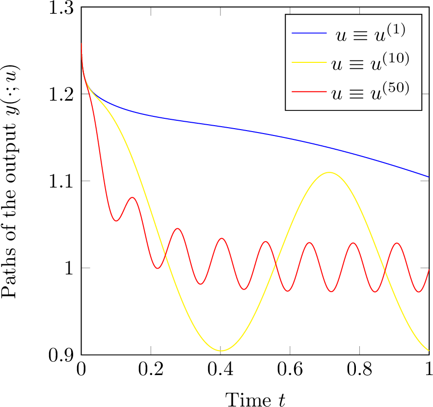
We show examples of the output in 25 using three different test controls from 26 , see Figure 1. Fixing \(k=1, 10, 50\) in this figure, we can see that functions that we try to reproduce by the signature model differ significantly. The first step now is to approximate \(y\) in 25 by \(y_S=CS(\cdot; u)\), where \(S(t; u):=S^N_{0,t}(\hat{U})\) is the truncated signature of order \(N\). This means that system 4 is considered with \(s_0=e_1\) and matrices \(A_0, A_1, \dots, A_m\) like in Proposition 6. We compute \(C\) according to the procedure explained in Section 5.1. We simulate \(\mathfrak n_u=1000\) paths of a standard Wiener process \(W\) and fix \(c_w=0.2\) to determine \(C\) from the least squares problem 22 . We check for the quality of the resulting matrix \(C\) by computing the following error \[\begin{align} \label{def95l295dis} \mathcal{E}_{\operatorname{sig}}:=\|y-y_S \|_{L^2}:=\sqrt{\frac{1}{1000} \sum_{k=1}^{1000} \int_0^T \|y(t; u^{(k)})- y_S(t; u^{(k)}) \|^2\mathrm{d}t}. \end{align}\tag{27}\] We intend to have a (bi)linearization error \(\mathcal{E}_{\operatorname{sig}}\) smaller than one percent. This can be achieved by setting \(N=5\) resulting in \(\mathcal{E}_{\operatorname{sig}}=3.7302\)e\(-03\). The signature approximation error is depicted by a red solid line in Figure 2. Having \(N=5\) leads to a truncated signature dimension of \(n=364\). This already provides a significant complexity reduction as we now deal with a bilinear system taking into account that \(S(\cdot; u)\) solves the bilinear system 4 with output \(y_S(\cdot; u) = C S(\cdot; u)\). Moreover, this bilinear system has a lower dimension than the original problem. We optimize the dimension of the \(n=364\)-dimensional system 4 further by applying the MOR procedure explained in Section 4. Analogue to 27 we define the signature dimension reduction error \(\mathcal{E}_{\operatorname{MOR}}:= \|y_S - \widecheck y_{S} \|_{L^2}\), where \(\widecheck y_{S}\) is the output of the reduced model 20 , and illustrate it in Figure 2 as well. The total error involving both the bilinearization and the MOR error is \(\mathcal{E}_{\operatorname{red}-\operatorname{sig}}:= \|y - \widecheck y_{S} \|_{L^2}\). \(\mathcal{E}_{\operatorname{red}-\operatorname{sig}}\) now depends on the dominant error of both approximations.

We observe from Figure 2 that the MOR error \(\mathcal{E}_{\operatorname{MOR}}\) is very large for \(r\leq 16\) since this error is above ten percent. Reduced order models with dimension \(20\leq r\leq 25\) perform with an error of around two percent but in such a scenario the MOR approach will still dominate the entire approximation, i.e., \(\mathcal{E}_{\operatorname{red}-\operatorname{sig}}=\mathcal{E}_{\operatorname{MOR}}\). Suddenly, \(r\geq 26\) basically leads to an exact reduced model when estimating the signature process. Therefore, we obtain \(\mathcal{E}_{\operatorname{red}-\operatorname{sig}}=\mathcal{E}_{\operatorname{sig}}\). The behavior of the MOR error follows the decay of the Hankel singular values introduced in Proposition 25. These are depicted in Figure [fig3]. This emphasizes that the Hankel singular values deliver an excellent a-priori criterion for the expected MOR error in our approach. In summary, we can say that we found a bilinear system 20 of dimension \(r=26\) that well-approximates a \(d=1000\)-dimensional system 24 with polynomial nonlinearities. This illustrates how powerful our approach can be.

6 Proofs of Section 3.1↩︎

We need the following lemma of Gronwall for the proofs below.

6.1 Proof of Lemma 9↩︎

6.2 Proof of Theorem 11↩︎

6.3 Proof of Theorem 12↩︎

Acknowledgments↩︎

MR and JW are supported by the DFG via the individual grant “Low-order approximations for large-scale problems arising in the context of high-dimensional PDEs and spatially discretized SPDEs”– project number 499366908.

References↩︎

---

1. University of Rostock, Institute of Mathematics, Ulmenstraße 69, 18057 Rostock, Germany, Email: martin.redmann@uni-rostock.de.↩︎

2. University of Rostock, Institute of Mathematics, Ulmenstraße 69, 18057 Rostock, Germany, Email: justus.werner@uni-rostock.de.↩︎