Incomplete U-Statistics of Equireplicate Designs:
Berry-Esseen Bound and Efficient Construction
October 23, 2025
Abstract
U-statistics are a fundamental class of estimators that generalize the sample mean and underpin much of nonparametric statistics. Although extensively studied in both statistics and probability, key challenges remain: their high computational cost—addressed partly through incomplete U-statistics—and their non-standard asymptotic behavior in the degenerate case, which typically requires resampling methods for hypothesis testing. This paper presents a novel perspective on U-statistics, grounded in hypergraph theory and combinatorial designs. Our approach bypasses the traditional Hoeffding decomposition, the main analytical tool in this literature but one highly sensitive to degeneracy. By characterizing the dependence structure of a U-statistic, we derive a Berry–Esseen bound valid for incomplete U-statistics of deterministic designs, yielding conditions under which Gaussian limiting distributions can be established even in degenerate cases and when the order diverges. We also introduce efficient algorithms to construct incomplete U-statistics of equireplicate designs, a subclass of deterministic designs that, in certain cases, achieve minimum variance. Beyond its theoretical contributions, our framework provides a systematic way to construct permutation-free counterparts to tests based on degenerate U-statistics, as demonstrated in experiments with kernel tests that use the Maximum Mean Discrepancy and the Hilbert–Schmidt Independence Criterion.
Keywords: degenerate U-statistics; dependency graph; hypergraph theory; kernel tests.
1 Introduction↩︎
U-statistics are a broad class of statistical estimators that extend the concept of the sample mean. Instead of simply averaging the observations, they average a symmetric, measurable function (kernel) of \(k > 1\) arguments over all \(\binom{n}{k}\) possible subsets of a sample of size \(n\). To mitigate the computational burden, Incomplete U-statistics [@blom1976some] consider only a subset, referred to as a design, of these \(\binom{n}{k}\) elements. While in principle the design can be strategically chosen to minimize the variance of the estimator, for ease of implementation, a random selection—either with or without replacement—is commonly used, despite not being the most efficient approach (see [@lee1990u], ch. 4.3).
The theoretical properties of U-statistics have been extensively studied in both Statistics [@lee1990u] and Probability [@korolyuk2013theory]. In particular, non-degenerate U-statistics have a Gaussian limiting distribution [@hoeffding1948u], while degenerate U-statistics converge to non-standard asymptotic distributions ([@lee1990u], ch. 3.2.3). For degenerate second-order U-statistics, i.e., when \(k=2\), [@gregory1977large] showed that the limiting distribution is an infinite weighted sum of centered \(\chi^2\) random variables. [@weber1981incomplete] extends the analysis to second-order degenerate incomplete U-statistics, demonstrating that both normal and weighted chi-square limiting behaviors can occur depending on the choice of the design. The latter non-standard distribution is often considered intractable for practical purposes; this is because the weights depend on the eigenvalues of a kernel-specific integral equation and, except for a few “nice” choices of the kernel function ([@lee1990u], ch. 6.2), this equation cannot be solved analytically.
On the applications side, U-statistics have found widespread use across various fields. These range from classical statistical estimation and inference tasks: e.g., in nonparametric hypothesis testing [@bergsma2014consistent; @yao2018testing], robust statistics [@joly2016robust; @MinskerWei2020], bootstrap and resampling methods [@leucht2013dependent; @bastian2024testing], to modern machine learning applications: e.g., in empirical risk minimization [@clemenccon2008ranking; @chen2023distributed], supervised learning ensembles [@mentch2016quantifying; @peng2022rates] and kernel methods [@gretton2005measuring; @gretton2012kernel; @liu2016kernelized]. Second-order U-statistics are the most common and widely used in practice. This class includes estimators of variance, covariance, Kendall’s Tau, Spearman’s Rho, Wilcoxon statistics, Cramer-Von Mises statistics. Additionally, they encompass novel estimators of the Maximum Mean Discrepancy (MMD) and the Kernel Stein Discrepancy, which are kernel methods designed for two-sample testing [@gretton2012kernel] and goodness-of-fit testing [@liu2016kernelized], respectively (see [@schrab2022efficient] for a discussion). Higher-order U-statistics are also relevant in applications, as they include estimators of dependence measures such as distance covariance [@szekely2007measuring], sign covariance [@bergsma2014consistent], and the Hilbert–Schmidt Independence Criterion (HSIC) [@gretton2005measuring].
Given the extensive applicability of U-statistics, there has been growing interest in studying incomplete U-statistics, both from a statistical perspective as in [@chen2019randomized; @sturma2024testing; @leung2026berry] and also from an applied machine learning perspective as in [@papa2015sgd; @clemenccon2016scaling; @schrab2022efficient], but there also remain significant challenges. On the one hand, selecting a design that minimizes variance is highly desirable, but it is a notoriously difficult combinatorial problem ([@lee1990u], ch. 4.3.2). Due to this challenge, researchers generally resort to random designs [@papa2015sgd; @clemenccon2016scaling; @chen2019randomized; @leung2026berry], which are easier to implement and analyze, but come at the cost of a suboptimal variance. On the other hand, the problem of determining the limiting distribution remains open. For instance, in the case of second-order degenerate incomplete U-statistics, no study has yet characterized how the limiting distribution transitions between normal and weighted chi-square laws, depending on the growth rate of the size of a minimum variance design. Addressing this gap is crucial for gaining a deeper understanding of the statistical properties of incomplete U-statistics and ensuring the validity of inferential procedures. Moreover, these theoretical insights would be essential for guiding practical applications, providing clear criteria for when a Gaussian approximation can be used or when resampling methods are required to approximate the limiting distribution.
In this paper, we present an efficient design construction and its asymptotic framework, to address the computational and statistical challenges posed by incomplete U-statistics. Our main contributions can be structured into four distinct points:
We show that the dependency graph [@baldi1989normal] of an incomplete U-statistic is the line graph of the design hypergraph.
We derive a new Berry–Esseen bound for incomplete U-statistics of deterministic designs, valid under the weakest assumptions known in the literature, using Stein’s method [@chen2004normal]. Moreover, we show that when both the maximum degree of the design hypergraph and the order \(k\) of the U-statistic are \(O(\log^q(n)\) for some \(q>0\), the bound converges to zero, ensuring asymptotic normality, even in the degenerate case and when the order diverges. Interestingly, these results are obtained without relying on the Hoeffding decomposition [@Hoeffding1961].
We develop efficient algorithms for constructing incomplete U-statistics based on equireplicate designs ([@lee1990u], ch. 4.3.2), a subclass of deterministic designs that tightly controls the maximum degree of the design hypergraph. The algorithms run in linear time in the design size and achieve minimum variance when \(k=2\). Our construction for \(k>2\) may be of independent interest to the combinatorial design and hypergraph communities.
We validate our theoretical results through numerical experiments on kernel-based test statistics, specifically the MMD and the HSIC. In a real-data application, we showcase a permutation-free variant of the MMD test that achieves substantial computational gains while matching the power and type I error control of its permutation-based counterpart, built on the same incomplete U-statistic.
Section 2 reviews background material and sets the notation for the paper. Section 3 derives a Berry–Esseen bound for incomplete U-statistics of deterministic designs and establishes conditions for Gaussian limiting distributions, even in the degenerate case and when the order diverges. Section 4 presents efficient algorithms for constructing equireplicate designs. Section 5 validates our theoretical results through extensive simulations on kernel-based test statistics and a real-data application presenting a permutation-free variant of the MMD test. Section 6 concludes with a summary and directions for future research. All proofs and technical details corresponding to each section of the main paper are provided in the supplemental materials at the end, where sections are labeled with an “S”. The R code for this paper can be found at https://github.com/CaesarXVII/IUstat_equireplicate_designs.
Existing works addressing convergence rates to limiting distributions of incomplete U-statistics that are most relevant to our setting and contributions include: [@rinott1997coupling], which examine a Markov-type dependence framework with applications to incomplete U-statistics; [@chen2019randomized], which consider randomized incomplete U-statistics in high-dimensional settings; [@sturma2024testing], which extend [@chen2019randomized] to a mixed degenerate setting with applications to testing a null hypothesis defined by equality and inequality constraints; [@kim2024dimension], which propose a new class of incomplete U-statistics that enable valid inference regardless of how the dimension scales with the sample size; [@shao2025u] that develop higher-order approximations for the sampling distribution of studentized non-degenerate incomplete U-statistics; and [@leung2026berry], which analyzes incomplete U-statistics of random designs—generated via Bernoulli sampling—across different regimes relating the sample size \(n\) and the expected design size. Among these prior works, none has provided a comprehensive framework encompassing: (i) finite-sample results on the distance to normality that account for both degenerate and non-degenerate cases; (ii) asymptotic analyses allowing the order \(k\) to grow with \(n\) and the design size to increase superlinearly in \(n\); and (iii) efficient algorithms for constructing minimum-variance designs when \(k=2\). Additional related work is discussed in 7.
2 Background and Notation↩︎
In this section, we introduce the necessary background and notation used throughout the paper. We strive for clarity and consistency in our notation, aligning it with the standard conventions in each of the domains we explore, namely U-statistics, combinatorial designs, and hypergraph theory. In particular, our notation and terminology for U-statistics closely follow [@lee1990u], for combinatorial designs we refer to [@ColbournDinitz2006] and [@wallis2016introduction], and for hypergraphs we primarily follow [@bretto2013hypergraph].
2.1 Incomplete U-statistics↩︎
Let \(X_1, \ldots, X_n\) be i.i.d. random variables taking values in a measurable space \((T, \mathcal{F})\) with common distribution \(P\). Consider the couple \((V,\mathcal{B}_k)\), where \(V = \{1, \ldots, n \}\) is the index set of the random variables and \(\mathcal{B}_k = \{ S \subseteq V, k \in V \mid \vert S \vert = k \}\) the collection of all subsets of \(V\) of size \(k\). Then, an incomplete U-statistic of order \(k\) can be written as:
\[U_{n,D}^{(k)} = \frac{1}{|D|} \sum_{ \{i_1, \ldots, i_k \} \in D} h( X_{i_1}, \ldots, X_{i_k}), \label{eq:IUk}\tag{1}\] where \(h: T^k \rightarrow \mathbb{R}\) is a fixed measurable kernel function that is symmetric in its arguments, i.e., \(h\left(x_1, \ldots, x_k\right)=h\left(x_{i_1}, \ldots, x_{i_k}\right)\) for every permutation \(i_1, \ldots, i_k\) of \(\{1, \ldots, k\}\) and \(D\subseteq \mathcal{B}_k\) represents the design of the incomplete U-statistics of size \(|D|\). If \(D = \mathcal{B}_k\), we obtain the complete \(k\)th-order U-statistic with \(|D| = \binom{n}{k}\). Likewise, in the combinatorial designs literature [@ColbournDinitz2006], the previously defined couple \((V,\mathcal{B}_k)\) identifies the complete (or trivial) \(k\)-design that considers only blocks of size \(k\).
For \(c\in \{0,1,2,\ldots, k\}\), let \(\mathcal{J}_c = \{ S_1, S_2 \in D \mid |S_1 \cap S_2 | = c \}\) be the set of all pairs of elements in the design which have \(c\) indices in common and denote \(f_c = |\mathcal{J}_c|\) its cardinality. Then, we can write the variance of an incomplete U-statistic of order \(k\) as:
\[\operatorname{Var} U_{n,D}^{(k)} =|D|^{-2} \sum_{c=0}^k f_c \; \sigma_c^2,\label{eq:var95ustat}\tag{2}\] where \(\sigma_c^2=\operatorname{Cov}\left(h\left(S_1\right), h\left(S_2\right)\right)\) with \(S_1, S_2 \in \mathcal{J}_c\) and \(h(S)\) is shorthand for \(h\left(X_{i_1}, \ldots, X_{i_k}\right)\), where \(S=\left\{i_1, \ldots, i_k\right\} \in D\). Moreover, by Theorem 4 in [@lee1990u] (page 15), we have:
\[\frac{\sigma_{b}^2}{b} \leq \frac{\sigma_{c}^2}{c} \label{eq:ineq}\tag{3}\]
for \(0 < b \leq c \leq k\) and \(b \in \{0, 1, \ldots, k\}\). In this work, we assume that \(\sigma_{k}^2 < \infty\). Combined with inequality 3 and the identity \(\sum_{c=0}^k f_c = |D|^{2}\), this assumption guarantees that \(\operatorname{Var} U_{n,D}^{(k)}\) is finite. Moreover, still by inequality 3 , if \(\sigma_c^2 = 0\), then it follows that \(\sigma_1^2 = \cdots = \sigma_{b}^2 = 0\) and the U-statistic is called degenerate of order \(c\). In this work, we assume \(\sigma_k^2 > 0\), which ensures that \(U_{n,D}^{(k)}\) can be at most degenerate of order \(k-1\). More generally, the order of the degeneracy determines the asymptotic distribution of the complete U-statistic. This is because \(\sigma_c^2 = 0\), implies that the first \(c\) terms vanish in the Hoeffding decomposition [@Hoeffding1961], which is a representation of a U-statistic of order \(k\) with a sum of uncorrelated U-statistics of order \(1, \ldots, k\). For example, when \(k=2\) and \(\sigma_1^2 = 0\), we have a first order degeneracy and [@gregory1977large] proved that \(n \;( U_{n,\mathcal{B}_2}^{(2)} - E[U_{n,\mathcal{B}_2}^{(2)}])\) converges in distribution to an infinite weighted sum of centered \(\chi^2\) random variables. However, if \(D \subset \mathcal{B}_k\), the limiting behavior of \(U_{n,D}^{(2)}\) can vary and crucially depends on the choice of the design [@weber1981incomplete].
2.2 Equireplicate designs↩︎
The class of equireplicate designs is the main focus of our paper. Within this class, every index occurs in the same number of elements of the design, usually called blocks. Any \(r\)-equireplicate design \(D\) based on \(V\), where the positive integer \(r\) denotes the replication parameter, satisfies:
\[|D| \; k = n \; r. \label{eq:equirep}\tag{4}\]
When \(k = 2\), incomplete U-statistics based on equireplicate designs achieve minimum variance, as demonstrated by Theorem 1 on page 195 of [@lee1990u]. When \(k > 2\), additional conditions are needed to ensure minimum variance, such as balanced incomplete block designs (BIBDs) and cyclic designs (see [@lee1982incomplete], Examples 2 and 7, respectively). Further details are provided in 8.1.
The existence of equireplicate designs requires specific divisibility conditions. In general, given a nonzero integer \(a\) and an integer \(b\), we write \(a \mid b\) to indicate that \(a\) divides \(b\), and \(a \nmid b\) otherwise. For our design constructions, we use modular arithmetic and some basic group theory (see [@gallian2021contemporary], ch. 2 for an overview). We write \(b \pmod n\) to denote the remainder upon dividing \(b\) by \(n\), but set \(b\pmod n\vcentcolon=n\) if the remainder is zero; we also write \(\text{gcd}(b,n)\) as the greatest common divisor of \(b\) and \(n\). In Section 4, we present efficient algorithmic constructions of equireplicate designs that use these algebraic concepts. Since we relabeled 0 as \(n\) when calculating values \(\pmod n\), we consider \(\mathbb{Z}_n=\{1,2,\ldots, n\}\) as the group of integers modulo \(n\) with additive identity element \(n\). This notation was chosen to ensure that the elements of our designs are labeled from the index set \(V=\{1,\ldots, n\}\).
2.3 Hypergraphs and deterministic designs↩︎
A hypergraph \(H\) is a couple \((V, E)\), where \(V\) is the vertex set, and \(E \subseteq \mathcal{P}(V)\setminus\{\varnothing\}\) is the hyperedge set, with \(\mathcal{P}(V)\) denoting the power set of \(V\). Each hyperedge \(e \in E\) is a non-empty subset of \(V\) and the singleton \(e_{v} = \{v\}\) represents a loop for all \(v \in V\). We call \(H(v)\) the set of hyperedges containing the vertex \(v\) and define the degree as \(d(v)=|H(v)|\) for all \(v \in V\). The average degree of a hypergraph \(H\) is denoted by \(\Bar{d}(H)\) and its maximum degree by \(\Delta(H)\). If each vertex has the same degree, we say that the hypergraph \(H\) is \(r\)-regular, which implies that \(\Bar{d}(H) = \Delta(H) = r\).
When every hyperedge contains exactly \(k\) vertices, i.e., \(|e| = k\) for all \(e \in E\), the hypergraph is called \(k\)-uniform. We can extend the classical handshaking lemma—that relates the number of edges in a graph with the sum of the degrees—to \(k\)-uniform hypergraphs. Indeed, for any \(k\)-uniform hypergraph \(H = (V, E)\), it holds that:
\[|E| \; k = \sum_{v \in V} d(v)\;, \label{eq:handshaking95kuni}\tag{5}\]
because each hyperedge contributes exactly \(k\) incidences, one for each vertex it contains.
To derive the Berry-Esseen bound and the asymptotic properties in section 3, we rely on a particular line graph construction. For a given hypergraph \(H = (V, E)\), its line graph \(L(H)\) is the couple \((E,E^{\prime})\) where \(E^{\prime} \;=\;\bigl\{\{e_i,e_j\} \;\bigm|\; e_i, e_j \in E \;\text{and}\; |e_i \cap e_j| \;\neq\;0 \bigr\}\). Note that our definition automatically includes loops, i.e., self-edges. In contrast, alternative definitions of the line graph explicitly exclude this possibility by imposing the additional condition \(e_i \neq e_j\) for any element of \(E^{\prime}\). In any case, \(L(H)\) is a graph, with vertex set that coincides with the hyperedge set of \(H\) and where an edge connects two vertices if and only if the corresponding hyperedges in \(H\) have at least one vertex in common.
A correspondence exists between \(k\)-uniform hypergraphs and deterministic designs1:
Observation 1. The hyperedge set of any \(k\)-uniform hypergraph identifies a deterministic design on the vertex set \(V\), and conversely, any deterministic design with building blocks of size \(k\) corresponds to the hyperedge set of a \(k\)-uniform hypergraph.
Because of this equivalence, any structural or theoretical insight gained in the hypergraph setting translates directly into properties of the corresponding designs and viceversa. Thus, for instance, the couple \((V, \mathcal{B}_k)\) can be interpreted either as the complete \(k\)-uniform hypergraph—commonly denoted by \(K_n^{(k)}\)—or as the complete \(k\)-design that underlies the complete \(k\)th-order U-statistic. More generally, given a deterministic design \(D\subseteq \mathcal{B}_k\), the couple \((V,D)\) defines the hypergraph of the design \(D\), which we denote by \(\mathcal{D} = (V,D)\). When \(D\subset \mathcal{B}_k\), \(\mathcal{D}\) is a sub-hypergraph of \(K_{n}^{(k)}\) and its hyperedge set \(D\) is the design of an incomplete U-statistic of order \(k\). By equation 5 , any deterministic design \(D\) defined over \(V\) must satisfy:
\[|D| \; k = n \; \Bar{d}(\mathcal{D})\;, \label{eq:deter}\tag{6}\]
where \(\Bar{d}(\mathcal{D})\) is the average degree of the hypergraph of the design \(D\). We rely on this result to express the size of a deterministic design as \(|D|=n\;\Bar{d}(\mathcal{D})/k\). Clearly, for an \(r\)-equireplicate design, \(\Bar{d}(\mathcal{D}) = r\) and equation (6 ) boils down to equation (4 ).
3 Normal Approximations of Incomplete U-statistics↩︎
An incomplete U-statistic can be seen as a classical mean computed in the space induced by the kernel function \(h\). Therefore, equation 1 can be expressed more concisely as:
\[U_{n,D}^{(k)} = \frac{1}{|D|} \sum^{}_{S \in D} h(S), \label{eq:IUk95red}\tag{7}\] where \(h(S)\) stays for the random variable \(h\left(X_{i_1}, \ldots, X_{i_k}\right)\) with \(S=\left\{i_1, \ldots, i_k\right\} \in D\).
The random variables in the set \(\left\{ h(S), \;S \in D \right\}\) are identically distributed since the data, \(X_1, \ldots, X_n\), are i.i.d., and \(h\) is a fixed, symmetric and measurable kernel function. Consequently, we denote \(E\left[h(S)\right] = \mu_{k}\) for all \(S \in D\) and, following the notation introduced in section 2.1, we can conclude that \(\operatorname{Var}[h(S)] = \sigma^{2}_{k}\) for all \(S \in D\). However, unlike in a standard i.i.d. mean estimation setting, the set may contain random variables which are dependent. The main insight that underpins all the results of this section is that we can tame this dependence by controlling \(\Delta(\mathcal{D})\), the maximum degree of the hypergraph of the design. This quantity has a simple interpretation: for a given design \(D\), \(\Delta(\mathcal{D})\) represents the index that appears most frequently in the design.
More specifically, in this section we characterize the dependence structure of an incomplete U-statistic through its dependency graph, which allows us to establish a Berry-Esseen bound that holds for all incomplete U-statistics of deterministic designs, even in the degenerate case. Leveraging this bound, we study the asymptotic properties of this class of statistics, when key parameters—such as the maximum degree \(\Delta(\mathcal{D})\) and the order \(k\)—are allowed to grow with \(n\). Overall, our results indicate that, among all deterministic designs of a given size, equireplicate ones should be preferred because they provide precise control over \(\Delta(\mathcal{D})\).
3.1 The dependency graph of incomplete U-statistics↩︎
The set \(\left\{ h(S), \;S \in D \right\}\) contains the random variables whose average defines \(U_{n,D}^{(k)}\), as shown previously in equation 7 . To characterize the dependence structure of this set, we define its dependency graph, a concept originally introduced in [@baldi1989normal] to derive normal approximations of distributions:
Definition 1. [Dependency graph] For a set of random variables \(\left\{ h(S), \;S \in D \right\}\) indexed by the vertices of a graph \(\mathcal{G}=(D, E)\), \(\mathcal{G}\) is said to be a dependency graph if, for any pair of disjoint sets \(\Gamma_1\) and \(\Gamma_2\) in \(D\) such that no edge in \(E\) has one endpoint in \(\Gamma_1\) and the other in \(\Gamma_2\), the sets of random variables \(\left\{h(S), S \in \Gamma_1\right\}\) and \(\left\{h(S), S \in \Gamma_2\right\}\) are independent.
In a dependency graph, there is an edge between two random variables only if they are dependent (absence of an edge implies independence). In the case of U-statistics, we include an edge between two random variables \(h(S_1)\) and \(h(S_2)\) if and only if \(S_1\cap S_2\neq\emptyset\).
Note that this corresponds with the definition of \(L(\mathcal{D})\), given in section 2.3:
Proposition 1. \(L(\mathcal{D})\) is the dependency graph of \(\left\{ h(S), \;S \in D \right\}\).
The maximum degree of the dependency graph \(\Delta(L(\mathcal{D}))\), bounds how many random variables each \(h(S)\) can be dependent with. Controlling this quantity is key for establishing a normal limiting distribution, as we demonstrate in the following section.
3.2 Berry-Esseen bounds for incomplete U-statistics↩︎
We begin by deriving an interpretable and tight upper bound for the maximum degree of the dependency graph \(\Delta(L(\mathcal{D}))\), expressed solely in terms of \(k\) and \(\Delta(\mathcal{D})\). This result is then combined with key findings from the literature on dependency graphs to establish a Berry–Esseen bound for incomplete U-statistics based on deterministic designs.
Intuitively, the maximum value of \(\Delta(L(\mathcal{D}))\) is attained when the block \(S\), which identifies the variable \(h(S)\), consists of indices that each appear with the highest possible frequency in the design; i.e., each has degree \(\Delta(\mathcal{D})\) in the hypergraph \(\mathcal{D}\). In this case, each of the \(k\) indices in \(S\) can contribute up to \((\Delta(\mathcal{D}) - 1)\) edges in the line graph (excluding the self-edge), yielding a total of at most \(k \;(\Delta(\mathcal{D}) - 1)\) dependencies for \(h(S)\). In contrast, the minimum value of \(\Delta(L(\mathcal{D}))\) is reached when only one index in the block \(S\) has degree \(\Delta(\mathcal{D})\), while the remaining \(k - 1\) indices do not appear in any other blocks. In this setting, \(h(S)\) is connected to exactly \((\Delta(\mathcal{D}) - 1)\) other variables in \(L(\mathcal{D})\). We formalize the upper and lower bounds—both of which are tight—in the following lemma.
Lemma 1. Let \(\mathcal{D} = (V, D)\) be the hypergraph of a deterministic design \(D\) and \(L(\mathcal{D})\) its line graph. Then, \[\Delta(\mathcal{D}) \leq \Delta(L(\mathcal{D})) \leq k\;(\Delta(\mathcal{D})-1) + 1 \; .\]
With this foundation, we can leverage powerful existing results from the literature on dependency graphs. In particular, we rely on [@chen2004normal] that couples Stein’s method with a concentration inequality to derive normal approximations under local dependence. Combining their findings with Lemma 1, we obtain a Berry-Esseen bound valid for all incomplete U-statistics based on deterministic designs.
Theorem 1 (Berry-Esseen for Deterministic Designs).
Let \(\left\{ h(S), \;S \in D \right\}\) be random variables indexed by the vertices of their dependency graph \(L(\mathcal{D})\), with \(D\) being a deterministic design. Assume that \(0< \sigma^{2}_{k} < \infty\) and that there exists \(2<p \leq 3\) such that \(E\left[\left|h(S) - \mu_k\right|^p \right] \leq \theta\) for some \(\theta>0\). Then,
\[\label{eq:berry95esseen} \sup _z\left|P\left(\frac{U_{n,D}^{(k)} - \mu_{k}}{\sqrt{\operatorname{Var}U_{n,D}^{(k)}}} \leq z\right)-\Phi(z)\right| \leq 75 \; \{k \;(\Delta(\mathcal{D})-1) + 1\}^{5(p-1)}\; \left(\frac{k}{n\;\Bar{d}(\mathcal{D})} \right)^{\frac{p}{2} - 1}\; \frac{\theta}{\sigma_k^p} \;\;\;.\tag{8}\]
As either \(k\) or \(\Delta(\mathcal{D})\) increase, while all other quantities are held fixed, the distance to normality grows. A similar effect occurs when the gap between the average degree \(\bar{d}(\mathcal{D})\) and the maximum degree \(\Delta(\mathcal{D})\) widens, which corresponds to deterministic designs whose associated hypergraph exhibits an increasingly skewed degree distribution.
Our Berry-Esseen bound distinguishes itself from existing results in the U-statistics literature by being valid in both degenerate and non-degenerate cases. It holds under minimal moment conditions on the kernel function \(h\) and makes explicit the critical role played by the order \(k\) and the maximum degree \(\Delta(\mathcal{D})\), both of which must be controlled to prevent deviations from normality. In contrast, existing works on convergence rates to limiting distributions for incomplete U-statistics either exclude the degenerate case altogether [@shao2025u], or address it under assumptions that are less interpretable than ours or stronger. For instance, [@rinott1997coupling] study the more general setting of weighted U-statistics but address the degenerate case only when \(k=2\), under comparatively less transparent assumptions. Likewise, [@kim2024dimension] focus on the second-order case and require the kernel to have a finite fourth moment to establish a Berry–Esseen bound for their cross U-statistics. [@chen2019randomized] derive Gaussian approximations valid for arbitrary order \(k\) and in high dimensions, but their results still rely on bounded polynomial moments of degree at least four and also [@sturma2024testing], who extend [@chen2019randomized] to a mixed-degenerate setting more in line with our unified framework, assume the kernel to be sub-Weibull. Finally, [@leung2026berry] establishes Berry–Esseen bounds for incomplete U-statistics under Bernoulli sampling—assuming a finite third moment of the kernel—however the analysis is limited to a fixed order \(k\).
Remark 1 (Berry-Esseen for bounded kernels). If the kernel is assumed to be bounded, such as the Gaussian kernel commonly employed in the MMD two-sample test [@gretton2012kernel], the bound in Theorem 1 can be sharpened by leveraging results from [@baldi1989normal], which have also been applied by [@cai2024asymptotic] that propose an independence test for high-dimensional data. We formally state and prove this tighter bound—most notably reducing the dependence on the maximum degree of the dependency graph from \(\Delta(L(\mathcal{D}))^{5(p-1)}\) to \(\Delta(L(\mathcal{D}))\)—in Theorem 5 of 9.
In addition, our approach departs from traditional methods in the U-statistics literature by focusing on the dependency graph of the random variables \(\left\{ h(S), \;S \in D \right\}\), thus operating directly in the space induced by the kernel function \(h\). This perspective allows us to entirely bypass the Hoeffding decomposition, which is the standard analytical tool but is sensitive to degeneracy. Notably, when the U-statistic is degenerate of order \(k-1\), the first \(k-1\) terms of the Hoeffding decomposition vanish, leaving only the highest-order component. In contrast, the dependency graph is not affected by such degeneracy, as it encompasses all types of dependencies, including those of order \(k\).
Note that the presence of any type of degeneracy still impacts the variance of an incomplete U-statistic. To establish 8 , we relied on a lower bound for \(\operatorname{Var}U_{n,D}^{(k)}\) that remains valid even under extreme degeneracy, specifically when \(\sigma^2_{k-1} = 0\). A comprehensive discussion on the variance of incomplete U-statistics of deterministic designs—including tight upper and lower bounds that involve \(\Bar{d}(\mathcal{D})\) and \(\Delta(\mathcal{D})\)—can be found in 9.5.
Among deterministic designs, equireplicate ones offer tight control over \(\Delta(\mathcal{D})\). In an \(r\)-equireplicate design \(\mathcal{D}^{\dagger}\), we have \(\Delta(\mathcal{D}^{\dagger}) = r\) since every index appears exactly \(r\) times. In the next Corollary of Theorem 1, we establish a Berry-Esseen bound specific to all incomplete U-statistics based on equireplicate designs.
Corollary 1. (Berry-Esseen for Equireplicate Designs). Let \(D^{\dagger}\) be an \(r\)-equireplicate design and assume that the conditions of Theorem 1 are met. Then,
\[\label{eq:be95equi} \sup _z\left|P\left(\frac{U_{n,D^{\dagger}}^{(k)} - \mu_{k}}{\sqrt{\operatorname{Var}U_{n,D^{\dagger}}^{(k)}}} \leq z\right)-\Phi(z)\right| \leq 75 \; \{k \;(r-1) + 1\}^{5(p-1)}\; \left(\frac{k}{n\;r} \right)^{\frac{p}{2} - 1}\; \frac{\theta}{\sigma_k^{p}} \;\;\;.\tag{9}\]
The result follows by substituting \(\Delta(\mathcal{D}) = \bar{d}(\mathcal{D}) = r\) in 8 , implying that there is no gap between the maximum and average degrees. Indeed, the hypergraph of an \(r\)-equireplicate design is \(r\)-regular, thus its degree distribution is a point mass at \(r\).
Moreover, Corollary 1 is valid for both degenerate and non-degenerate cases, and the bound in 9 is tighter for incomplete U-statistics based on \(r\)-equireplicate designs than the bound in 8 for U-statistics based on non-equireplicate deterministic designs of the same size (see Remark 2 for a detailed explanation).
Remark 2. We can compare the maximum degree of the dependency graph for an incomplete U-statistic based on an \(r\)-equireplicate design \(D^{\dagger}\) with that of one based on a non-equireplicate design \(D\). Specifically, if \(k\;(r - 1) + 1 < \Delta(\mathcal{D})\), then it must follow that \(\Delta(L(\mathcal{D}^{\dagger})) < \Delta(L(\mathcal{D}))\) by Lemma 1. When \(k = 2\) i.e., for second-order U-statistics, this condition is unnecessary: if both designs have the same size, the \(r\)-equireplicate one always yields a lower maximum degree in the dependency graph and is therefore preferable for minimizing dependence. Furthermore, when \(|D^{\dagger}| = |D|\), we also have that \(r = \Delta(\mathcal{D}^{\dagger})< \Delta(\mathcal{D})\) for any value of \(k\). These results are formally stated and proved in Proposition 3 and Lemma 3, both presented in 9.
Remark 3. [Berry-Esseen bound for equireplicate and linear designs] In the proof of Theorem 1, we also obtain a bound that improves upon 8 whenever there exists a \(c \in \{1, \ldots, k-1\}\) such that \(f_c > 0\) and \(\sigma_c^2 > 0\). This refined bound is applied in Corollary 3 to derive a tighter result—valid in the non-degenerate case—for the class of equireplicate and linear designs. The term “linear” refers to the associated hypergraph \(\mathcal{D}^{\diamond} = (V, D^{\diamond})\), in which for all \(S_1, S_2 \in D^{\diamond}\) with \(S_1 \neq S_2\), we have that \(\left|S_1 \cap S_2\right| \leq 1\). That is, any pair of random variables in the set \(\left\{ h(S), \;S \in D^{\diamond} \right\}\) shares at most one index.
3.3 Asymptotic results in the finite and infinite order regimes↩︎
Theorem 1 provides a Berry-Esseen bound for all incomplete U-statistics based on deterministic designs. To ensure convergence to a normal distribution, both the order \(k\) and the maximum degree \(\Delta(\mathcal{D})\) must grow slowly with the number of observations \(n\), as suggested by 8 . This requirement is formalized in the central limit theorem below, where \(k\) represents a sequence of natural numbers indexed by \(n\).
Theorem 2. (CLT for Incomplete U-statistics of Deterministic Designs).
Let \(\{ h_k(S), \;S \in D^{(k)}_n \}\) be a sequence of sets of random variables, with each set indexed by the vertices of its dependency graph \(L(\mathcal{D}^{(k)}_n)\), with \(D^{(k)}_n\) being a sequence of deterministic designs of growing size that identifies the sequence of hypergraphs \(\mathcal{D}^{(k)}_n = (V,D^{(k)}_n)\). Moreover, assume that \(0 < \sigma^{2}_{k} < \infty\) for all \(k\), that there exists \(\epsilon >0\) such that \(E\left[\left|h_k(S) -
\mu_k\right|^{2+\epsilon} \right] \leq \theta_k\) with \(\theta_k>0\) for all \(k\) and that \(\max\{k,\;\Delta(\mathcal{D}^{(k)}_n),\;
\theta_k\}=O(\log^q(n))\) with \(q >0\). Then, as \(n \rightarrow \infty\), we have
\[\label{eq:clt} \frac{U_{n,D^{(k)}_n}^{(k)} - \mu_{k}}{\sqrt{\operatorname{Var}U_{n,D^{(k)}_n}^{(k)}}} \xrightarrow{\;\;d\;\;} \mathcal{N}(0,1) \;.\tag{10}\]
The proof, provided in 9, is based on the Berry-Esseen bound of Theorem 1. To our knowledge, Theorem 2 is the first asymptotic result in the U-statistics literature that simultaneously covers both the degenerate and non-degenerate cases, and is valid in both the finite-order regime (where \(k\) is fixed) and the infinite-order regime (where \(k\) grows with \(n\)), thus providing a unified theoretical framework with minimal assumptions.
However, a generic sequence of deterministic design \(D^{(k)}_n\) may not respect the condition \(\Delta(\mathcal{D}^{(k)}_n)=O(\log^q(n))\) required for Theorem 2 to hold. Specifically, this happens when a hypergraph \(\mathcal{D}\) has an unbalanced degree distribution, as shown in the following example.
Example 1 (Designs with unbalanced degree distribution). Consider a \(k\)-uniform star design (see Definition 1.10 in [@keevash2014spectral], with \(t=1\)). When \(k=2\), the hypergraph \(\mathcal{D}^{\star}\) is a star graph with \(n\) vertices. By construction, the center of the star is the index with the maximum degree \(\Delta(\mathcal{D}^{\star}) = n-1\). Therefore, when \(n\) diverges, an incomplete U-statistic based on the star graph violates the conditions of Theorem 2, that guarantee an asymptotically normal distribution only when \(\Delta(\mathcal{D})\) grows slowly with \(n\).
On the other hand, for an equireplicate design, the parameter \(r\) determines the order of growth of the entire degree distribution of its associated hypergraph. This allows for considerable flexibility in the design construction as \(r\) can be chosen to grow at a desired rate with \(n\)—such as the \(O(\log^q(n))\) of Theorem 2—and even be fixed as \(n\) diverges.
In the next paragraphs, we compare Theorem 2 with existing results in the literature, highlighting its key features in both order regimes and further justifying the choice of equireplicate designs among deterministic ones. In our simulation studies of Section 5, we focus on the finite-order regime, which is relevant for kernel-based hypothesis testing.
Finite-order regime. When \(k\) is fixed, we omit the subscript and the superscript \(k\), referring simply to the kernel function \(h\) and the design \(D_n\). Thus, with minimal moment conditions on \(h\) and by requiring that the maximum number of dependencies in the set \(\left\{ h(S), \;S \in D_n \right\}\) grows at most with a logarithmic rate, Theorem 2 ensures asymptotic normality—even in the degenerate case—while preserving the classical computational advantages of incomplete U-statistics. This is because, any deterministic design \(D_n\) satisfies \(|D_n| = n \Bar{d}(\mathcal{D}_n)/k\) by equation 6 . Thus, since we assumed that \(\Delta(\mathcal{D}_n)=O(\log^q(n))\), then \(|D_n| = O(n \log^q(n))\) because \(\Bar{d}(\mathcal{D}_n) \leq \Delta(\mathcal{D}_n)\) by definition of the maximum degree.
Moreover, from the Berry–Esseen bound in 8 with \(p = 3\), it follows that under the assumptions of Theorem 2, the convergence rate to the standard normal distribution is \(n^{-1/2}\), up to logarithmic factors (see the proof of Theorem 2 for details). This rate matches the classical Berry–Esseen bound for the complete U-statistic in the finite-order non-degenerate case (see [@lee1990u], ch. 3.3 and references therein), again up to logarithmic terms. It is also only slightly slower than the \(o(n^{-1/2})\) rate established in [@korolyuk1989convergence] for the complete U-statistic in the finite-order degenerate case, where the limiting distribution is non-Gaussian. In that setting, the variance scales as \(n^{k/2}\) for the complete statistic, while for the incomplete one it scales as \(|D_n|^{1/2}\) (see Corollary 2). This last result confirms—and extends to deterministic designs—the findings of Remark 3.2 in [@chen2019randomized], which were stated for random designs.
Besides, existing results on normal approximations in the finite-order regime—such as [@chen2019randomized]—have to rely on bootstrap methods in practice to estimate the variance, which can increase the computational burden. On the contrary, our central limit theorem in 10 is readily applicable in the most extreme case of degeneracy—namely, of order \(k-1\)—for incomplete U-statistics based on equireplicate designs, as shown in Corollary 2. This setting is particularly relevant for hypothesis testing problems, including kernel-based tests, that we tackle in our simulation studies of Section 5.
Corollary 2 (CLT degenerate case of order \(k-1\) for equireplicate designs).
Let \(D^{\dagger}_n\) be a sequence of \(r\)-equireplicate designs, assume that \(0 = \sigma_1^2 = \cdots = \sigma_{k-1}^2\) and that all the conditions of Theorem 2 are satisfied with \(k\) fixed. Then, as \(n \to \infty\), we have
\[\label{eq:clt95dege95equi} \sqrt{\frac{n \; r_n}{k}}\;\;\frac{U_{n,D^{\dagger}_n}^{(k)} - \mu_{k}}{\sigma_k} \xrightarrow{\;\;d\;\;} \mathcal{N}(0,1) \;.\tag{11}\]
The result follows from Theorem 2. This is because \(\Delta(\mathcal{D}_n) = r_n = O(\log^q(n))\) by assumption, and the variance simplifies to \(\operatorname{Var}U_{n,D^{\dagger}_n}^{(k)} = \sigma^2_k/|D^{\dagger}_n|\) by applying the lower bound in Lemma 2. The final expression then follows by substituting \(\operatorname{Var}U_{n,D^{\dagger}_n}^{(k)}\) in 10 , with \(|D^{\dagger}_n|\) determined by equation 4 . If the kernel is further assumed to be bounded, we can allow \(r_n = O(n^{1/4})\) in 11 , as explained in the proof of Theorem 5 of 9.
Proposition 2 shows that \(\sigma^2_k\) can be consistently estimated with the sample variance \(s^2_k\) calculated over the set \(\left\{ h(S), \;S \in D^{\perp}_n \right\}\), which contains i.i.d. random variables that do not have indices in common. More specifically, if \(k \mid n\), \(D^{\perp}_n\) is an equireplicate design with \(r=1\) and thus of size \(n/k\) by equation 4 2. For instance, fixing \(n=9\) and \(k=3\), we can consider the set \(\left\{ h\left(X_1, X_2, X_3\right),h\left(X_4, X_5, X_6\right), h\left(X_7, X_8, X_9\right) \right\}\) to calculate \(s^2_k\). The choice of this estimator for \(\sigma^2_k\) makes the implementation of 11 straightforward in practice, with negligible additional computational cost due to the estimation step.
Proposition 2. Assume that \(k \mid n\) and that all the conditions of Corollary 2 are satisfied. Consider the set \(\left\{ h(S), \;S \in D^{\perp}_n \right\}\), where \(D^{\perp}_n\) is a sequence of \(1\)-equireplicate designs of size \(n/k\). Let \(s^2_k\) be the standard unbiased sample variance estimator calculated over \(\left\{ h(S), \;S \in D^{\perp}_n \right\}\). Then \(s^2_k \xrightarrow{p} \sigma^2_k\).
Remark 4 (CLT for equireplicate and linear designs). The variance scaling factor in Theorem 2 becomes specific to each deterministic design if there exists a \(c \in \{1, \ldots, k-1\}\) such that \(f_c > 0\) and \(\sigma^2_c > 0\). In this case, determining the asymptotic behavior of the incomplete U-statistic requires analyzing how the nonzero \(f_c\) terms grow with the sample size. In Corollary 4, we provide such a result, establishing a CLT for the class of equireplicate and linear designs. Note that Corollary 4 is valid for any equireplicate design when \(k=2\) because they are also linear, since no pair of distinct blocks \(S_1\) and \(S_2\) in \(\mathcal{B}_2\) can share more than one element. However, to apply Theorem 2 in practice, it is necessary to estimate the nonzero \(\sigma^2_c\) terms. This is a well-studied problem, and several methods are available in the literature, including consistent covariance estimators, jackknife, and bootstrap techniques (see ch. 5.3 of [@lee1990u] for an overview).
Infinite-order regime. Recently, infinite-order U-statistics (IOUS) have attracted growing attention in the statistics and machine learning communities, particularly due to their relevance in uncertainty quantification for supervised learning ensembles (see e.g., [@mentch2016quantifying; @peng2022rates]). Theorem 2 contributes to this increasingly active and important area of research by providing the first result on incomplete U-statistics that considers a diverging order \(k\), even in the presence of degeneracy. The only related works on IOUS in the incomplete setting are [@SongChenKato2019], which develops distributional approximations for high-dimensional, non-degenerate IOUS and [@sturma2024testing], that extends [@SongChenKato2019] to a mixed-degenerate setting. However, their analyses rely on the Hoeffding decomposition, which becomes problematic in the IOUS regime. Specifically, when assuming \(\sigma^2_k < \infty\), the first-order term in the decomposition—known as the Hájek projection—vanishes as \(k \to \infty\), significantly complicating the analysis. This issue arises from inequality 3 , which implies \(k\sigma^2_1 < \sigma^2_k\). Hence, if \(\sigma^2_k\) is bounded and \(k\) diverges, we necessarily have \(\sigma^2_1 = O(k^{-1})\). As a result, the variance of the Hájek projection shrinks to zero, and controlling the moments of an increasing number of degenerate terms becomes challenging, as noted by [@SongChenKato2019].
Our approach avoids these complications as it does not rely on the Hoeffding decomposition and instead operates directly in the space induced by the kernel function \(h\). Consequently, it remains valid in both degenerate and non-degenerate cases without imposing assumptions on the order of the \(\sigma^2_c\) terms in equation 2 . The only additional requirement in the infinite-order regime is a logarithmic growth condition on \(\max\{k,\theta_k\}\), making our framework particularly interesting for the IOUS setting. Under the conditions of Theorem 2, the computational efficiency of incomplete U-statistics is preserved even in the infinite-order regime, by the same reasoning outlined for the finite-order case.
Remark 5. The logarithmic growth condition in Theorem 2 can be relaxed to a polynomial growth condition, provided the polynomial degree remains sufficiently small. Indeed, allowing \(\max\{k,\;\Delta(\mathcal{D}^{(k)}_n),\; \theta_k\}=O(n^{1/q})\), with \(q > 22/\epsilon + 21\) and \(0 < \epsilon \leq 1\), still ensures a standard Gaussian limiting distribution for the centered and rescaled incomplete U-statistics, provided that the other conditions of Theorem 2 are satisfied (see the proof in 9 for further details). However, imposing a logarithmic growth condition offers two advantages: it recovers the classical Berry-Esseen \(n^{-1/2}\) convergence rate to the standard normal distribution—up to logarithmic factors—even in the infinite-order regime when \(\epsilon=1\), and it retains linear computational complexity in \(n\) for any deterministic design \(D^{(k)}_n\), again up to logarithmic terms, in both finite and infinite-order settings.
Remark 6. To apply Theorem 2 in the infinite-order regime, we need a consistent estimator of the variance when \(k\) diverges. Existing works have proposed variance estimation methods for incomplete U-statistics in the infinite-order regime, which can be applied [@wang2014variance; @SongChenKato2019; @xu_var_est_rf_2024]. However, specific details for implementation of our framework in this regime is left for future work.
4 Efficient Construction of Equireplicate Designs↩︎
In this section, we highlight another major advantage of equireplicate designs: they can be constructed in linear time with respect to the design size.
For second-order incomplete U-statistics, equireplicate designs of any given size can be efficiently constructed and have minimum variance. Therefore, equireplicate designs should be preferred when \(k=2\), the most common and widely used case in practice.
When \(k > 2\), constructing equireplicate designs becomes challenging, as it relates to open problems in discrete mathematics. In Section 4.2 we present a construction which has still a linear computational complexity in the design size—when \(k\) is fixed—and that allows \(|D| = O(n^2)\) (see Remarks 9 and 8 for further details). This construction, based on cyclic permutations (see [@lee1982incomplete], Example 7), may be of independent interest for the combinatorial design and hypergraph community.
4.1 Construction of r-equireplicate designs when k = 2↩︎
For second-order incomplete U-statistics, an \(r\)-equireplicate design is a subset of \(\mathcal{B}_2\) of size \(|D|=nr/2\), such that each index appears in exactly \(r\) pairs. Our approach relies on a partition of \(\mathcal{B}_2\) into disjoint \(1\)-equireplicate designs when \(n\) is even (\(2 \mid n\)), and into disjoint \(2\)-equireplicate designs when \(n\) is odd (\(2 \nmid n\) and thus \(2 \mid r\) by equation 4 if the design exists). In both cases the whole partition can be generated sequentially, allowing us to obtain an \(r\)-equireplicate design by taking the union of a prescribed number of subsets from it. Algorithms 1 and 2 implement this procedure for even and odd \(n\), respectively. Theorem 3 establishes that these algorithms have linear computational complexity in the design size and that the resulting incomplete U-statistics achieve minimum variance. Additional details are provided in 10.1. That section also discusses the connections between our algorithms and factorizations of the complete graph \(K^{(2)}_n\).
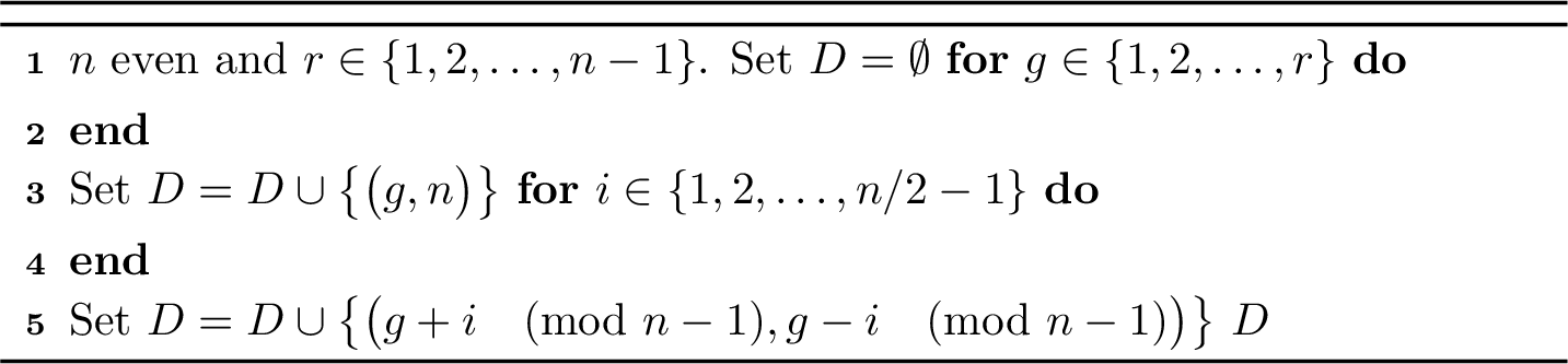

Theorem 3 (Equireplicate Designs with Minimum Variance when \(k=2\)). Let \(n\) be an integer and consider the designs produced by Algorithms 1 and 2. If \(n\) is even and \(r \in \{1,2,\ldots,n-1\}\), the output of Algorithm 1 is an \(r\)-equireplicate design, \(D\). If \(n\) is odd and \(r \in \{2,4,6,\ldots,n-1\}\), the output of Algorithm 2 is an \(r\)-equireplicate design, \(D\). In both cases, the algorithm runs in \(O(nr)=O(|D|)\) time. Moreover, the variance of the corresponding incomplete U-statistic satisfies \(\operatorname{Var} U_{n,D}^{(2)} = |D|^{-1} \{ 2(r-1)\sigma_1^2 + \sigma_2^2 \}\), which is minimal among all incomplete U-statistics with the same design size \(|D|\).
Remark 7. The accompanying code of this paper, implements Algorithms 1 and 2 in a fully vectorized manner in R, resulting in highly efficient execution. For example, with \(n = 10^6\) and \(r = 10^2\), Algorithm 1 completes in approximately 62 seconds, while Algorithm 2 requires about 72 seconds for \(n = 10^6 + 1\) with the same \(r = 10^2\). The experiment was conducted on a laptop equipped with an Intel i7-6700HQ CPU @ 2.60 GHz and 16 GB of RAM. Additional speedups could be achieved through parallelization over either of the for-loops, although this has not yet been implemented.
4.2 Construction of r-equireplicate designs when k > 2↩︎
For incomplete U-statistics of order \(k\), an \(r\)-equireplicate design is a subset of \(\mathcal{B}_k\) of size \(|D|=nr/k\), such that each index appears in exactly \(r\) blocks. Our approach relies on a partial partition of \(\mathcal{B}_k\) into disjoint \(k\)-equireplicate designs (hence \(k \mid r\)). This partition can be generated sequentially, allowing us to obtain an \(r\)-equireplicate design by taking the union of a prescribed number of subsets from it. Algorithm 3 implements this procedure and Theorem 4 shows that, for any strictly increasing sequence of natural numbers \(\eta(\cdot)\), if \(n > 3\;\eta(k-1)\;\{\eta(k-1) - \eta(0)\}\) and \(r\in \{k,2k,\ldots,\phi(n)k \}\), then Algorithm 3 constructs \(r\)-equireplicate designs with linear computational complexity in the design size. In both the algorithm and theorem, we denote by \(\mathcal{C}_n = \{ a \in \mathbb{Z}_n| \; \text{gcd}(a,n) = 1 \}\) the set of coprimes of \(n\) and with \(\phi(n) = \mid \mathcal{C}_n \mid\) its cardinality, which is known as Euler’s totient function. Additional details are provided in 10.2, which also explores connections between our algorithm and factorizations of the complete \(k\)-uniform hypergraph \(K_n^{(k)}\).

Theorem 4. [Equireplicate Designs when \(k>2\)]
Let \(k > 2\), \(\eta: \{0, \ldots, k-1\} \to \mathbb{N}_0\) be any strictly increasing natural number valued sequence, \(n\) be a positive integer such
that \(n > 3\;\eta(k-1)\;\{\eta(k-1) - \eta(0)\}\) and \(r\in \{k,2k,\ldots,\phi(n)k \}\). Then, the output of Algorithm 3 is an \(r\)-equireplicate design \(D\) and the runtime of Algorithm 3 is \(O(nr)=O(|D|)\).
Remark 8 (Order of \(|D|\) and choice of \(\eta(\cdot)\)).
When \(\eta(j) = 2^j\) in Algorithm 3, our construction is related to the one proposed in [@shao2025u]. However, the order of the corresponding design size is not explicitly derived in that work. In contrast, Theorem 4 shows that in our setting \(r = O(\phi(n) k)\), which—by equation 4 —implies \(|D| = O(n\;\phi(n))\). Following [@hardy2008introduction], \(\phi(n)\) is asymptotically of order \(n\) and, when \(n\) is prime, \(\phi(n)\) attains its maximum value of \((n-1)\). Thus, Algorithm 3 constructs an \(r\)-equireplicate design of size \(|D| = O(n^2)\), regardless of the specific choice of \(\eta(\cdot)\). However, choosing the right \(\eta(\cdot)\) remains important, as it determines the degree of overlap between the blocks forming the design and thereby influences the variance of the resulting incomplete U-statistics. A theoretical analysis of this choice, quantifying its impact on the variance, is left for future work.
5 Numerical Experiments↩︎
In this section, we empirically validate the theoretical results established in Section 3.3 regarding the asymptotic distribution of incomplete U-statistics of equireplicate designs in the finite order regime. We also investigate key aspects of our novel algorithms for constructing such equireplicate designs, introduced in Section 4, with particular focus on their variance-minimization property (when \(k=2\)) and linear computational complexity.
To this end, we conduct two sets of simulation studies on kernel-based testing methods: one on the two-sample test based on the unbiased MMD (uMMD) statistic, which is a second-order U-statistic (i.e., covering the \(k=2\) case), and the other on the independence test based on the HSIC [@gretton2007kernel], which is a fourth-order U-statistic (i.e., covering the \(k>2\) case). In addition, we illustrate our methodology on the widely used CIFAR-10 image classification dataset [@Krizhevsky09learningmultiple], which has frequently served as a benchmark for evaluating alternatives to the standard MMD two-sample test (see e.g., [@liu2020learning]). In this context, our novel approach provides a permutation-free version of the MMD test, that offers substantial computational advantages.
5.1 MMD experiments↩︎
In the first study, we perform a series of two-sample tests using incomplete versions of the uMMD test statistic—constructed via equireplicate designs—to assess departures from normality in their asymptotic distributions. Under the null \(H_0\)—i.e., when the two samples are drawn from the same distribution—the complete uMMD statistic (see eq. (6) in [@gretton2006kernel]) is a degenerate U-statistic and has a non-Gaussian limiting distribution. Under the alternative \(H_1\), it is non-degenerate and converges to a normal (see Theorem 8 in [@gretton2006kernel] for details).
More specifically, we simulate each time both samples \((X,Y)\) i.i.d. from a \(\mathcal{N}(0,1)\). We vary the common sample size \(n \in \{100, 200, 400,800,1600\}\). Each incomplete uMMD statistic is computed using a linear kernel and an \(r\)-equireplicate design generated by Algorithm 1. We select \(r \in \{1,\log(n),\log^2(n),\log^3(n), n/2, n-1\}\). We obtain the empirical distribution of the standardized uMMD statistic by repeating the experiment \(500\) times, standardizing the statistic in each replicate using its Monte Carlo estimate of the standard deviation. To quantify departures from normality, we compute the Kolmogorov-Smirnov (KS) distance between each empirical distribution and \(\mathcal{N}(0,1)\). We then repeat the entire procedure \(100\) times to produce a sampling distribution of KS distances. The left panel in Figure 4, reports \(95\%\) Monte Carlo confidence intervals (CI) for the KS distance (centered at the corresponding mean) and, for reference, shows \(Q_{0.975}\) and \(Q_{0.5}\), the \(97.5\%\) and \(50\%\) quantiles of the KS distance when the data are truly \(\mathcal{N}(0,1)\), respectively.
We observe that for \(r \in \{\log (n),\, \log^2 (n)\}\), the KS CIs lie below \(Q_{0.975}\) even at \(n=100\) and quickly contract toward \(Q_{0.5}\) as \(n\) increases. When \(r=\log^3(n)\), a larger sample size is required before the upper bound drops below \(Q_{0.975}\), but the decreasing trend is evident. In contrast, for larger values of \(r\) (e.g., \(r=n/2\)), the distance to normality remains roughly constant as \(n\) grows3. These findings validate Theorem 2 for \(k=2\), which predicts that for \(r=O(\log^q (n))\) (with fixed \(q\)), deviations from normality are small and diminish as \(n\) increases.
In practice, a Monte Carlo estimate of the uMMD standard deviation is not available. However, since the uMMD is degenerate under \(H_0\), we can use the variance estimator of Proposition 2. Figure 9 in 11 replicates Figure 4 but standardizes by \(s_2^2\) rather than by a Monte Carlo standard deviation. The results are virtually identical, thus using this estimator does not materially affect the KS CI as predicted by Corollary 2.
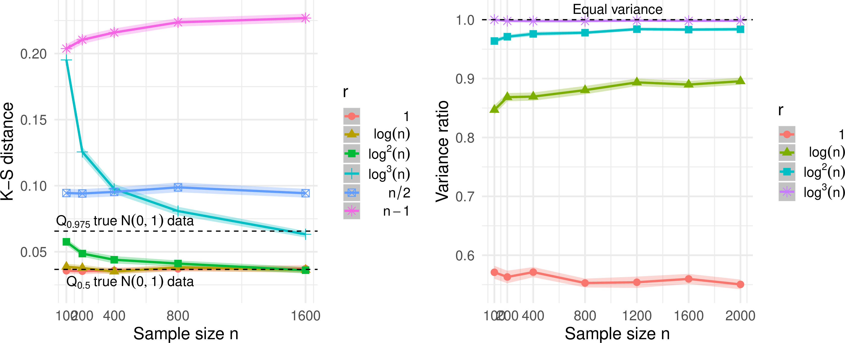
In the second study, we compare the variance of the uMMD statistic computed under equireplicate designs with that under random designs, to verify that with the equireplicate designs produced by Algorithm 1 we achieve minimum variance. To this end, we perform another series of two-sample tests, this time drawing the two samples from different distributions so that the uMMD statistic is non-degenerate.
More specifically, we simulate each time \(X \overset{iid}{\sim} \mathcal{N}(0,1)\) and \(Y \overset{iid}{\sim} \mathcal{N}(2,1)\). We vary \(n \in \{100, 200, 400,800,1200, 1600, 2000\}\) and select \(r \in \{1,\log(n),\log^2(n),\log^3(n)\}\). We follow the same procedure as in the first study to obtain Monte Carlo estimates of the variance of the uMMD statistic under both equireplicate and random designs. We then take their ratio (equireplicate/random) as a measure of relative efficiency and repeat the entire experiment \(100\) times to obtain a sampling distribution of variance ratios. The right panel of Figure 4 reports \(95\%\) Monte Carlo CI for these ratios, together with a reference line at \(1\), which corresponds to equal variance. We observe that the upper bounds of all CIs lie below \(1\), with a single exception at \(r=\log^{3}(n)\) when \(n=100\): in this case \(r \approx n-1\), so the statistic is effectively the complete uMMD and the variances coincide. As \(r\) increases, the efficiency gains diminish but appear to stabilize at a strictly positive level as \(n\) grows. These findings validate Theorem 3, confirming that the designs produced by Algorithm 1 achieve the minimum-variance property.
5.2 HSIC experiments↩︎
Following the same approach of the first MMD study, we conduct a series of independence tests using incomplete versions of the unbiased HSIC (uHSIC) statistic—constructed via equireplicate designs—to assess deviations from normality in their asymptotic distributions. Under \(H_0\)—i.e., when the two samples are independent—the complete uHSIC statistic (see the \(\mathrm{HSIC}_s(Z)\) definition in [@gretton2007kernel]) is degenerate of order \(1\) and has a non-Gaussian limiting distribution. Under \(H_1\), it is non-degenerate and converges to a normal (see Theorem 1 and 2 in [@gretton2007kernel] for details).
More specifically, we simulate each time both samples \((X,Y)\) i.i.d. from a \(\mathcal{N}(0,1)\). We choose \(n \in \{200, 400,800,1600\}\). The incomplete uHSIC statistic is computed from eq. (23) of [@schrab2025practical], accounting for kernel symmetrization, using a linear kernel and an \(r\)-equireplicate design constructed by Algorithm 3, with \(k=4\) and \(\eta(j)=2^j\) (see Remark 8). We select \(r \in \{1,\log(n),\log^2(n),\log^3(n)\}\)4. We obtain a sampling distribution of the KS distance between the empirical distribution of the standardized uHSIC statistic and \(\mathcal{N}(0,1)\) as described in the first MMD study. The left panel in Figure 5, reports \(95\%\) Monte Carlo CI for the KS distance and, for reference, shows \(Q_{0.975}\) as well as \(Q_{0.5}\).
We observe that for \(r \in \{\log(n),\, \log^2(n),\, \log^3(n)\}\), the KS CI lie below \(Q_{0.975}\) even at \(n=200\) and contract rapidly toward \(Q_{0.5}\) as \(n\) increases. The case \(r=\log^3(n)\) shows a slower decrease toward \(Q_{0.5}\), although the downward trend is evident. These findings support Theorem 2 for \(k>2\) (in particular \(k=4\)), which predicts that for \(r=O(\log^q(n))\) with fixed \(q\), deviations from normality remain small and vanish as \(n\) grows.
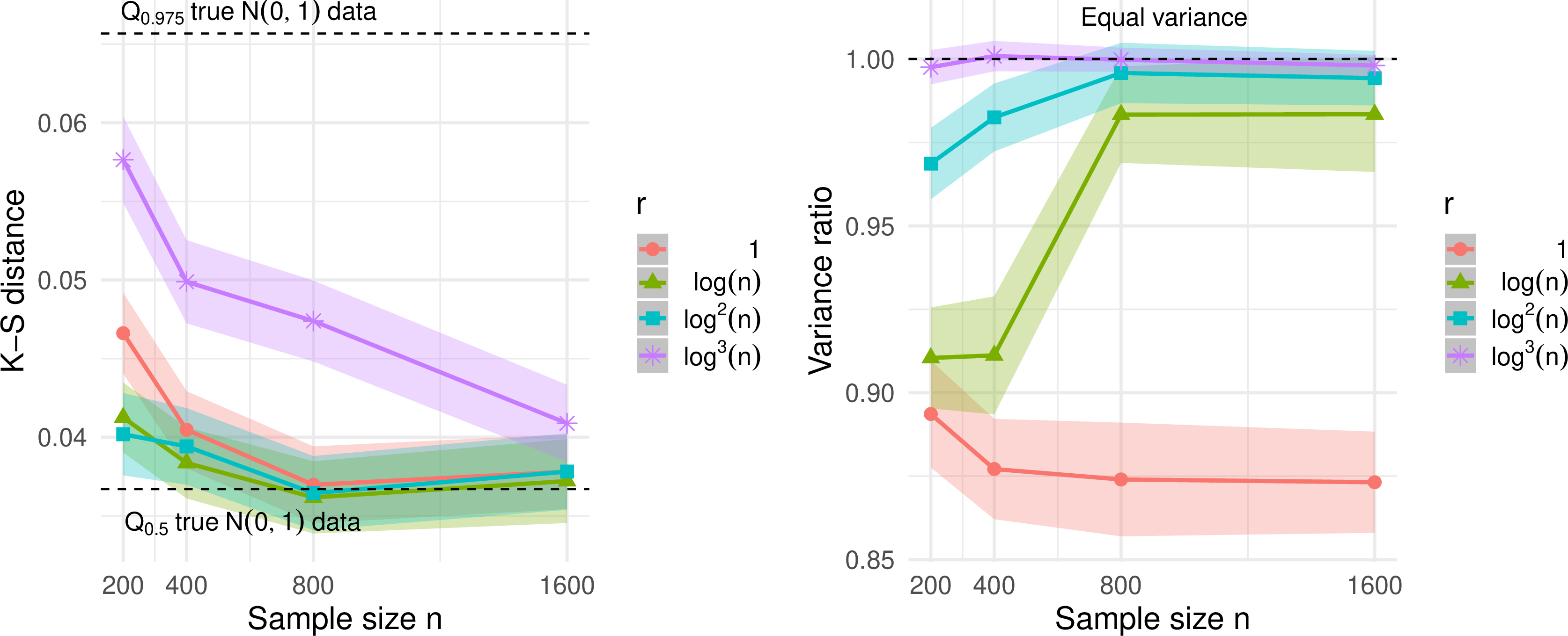
Following the same approach of the second MMD study, we compare the variance of the uHSIC statistic computed under equireplicate designs with that under random designs, to verify that incomplete U-statistics based on the equireplicate designs produced by Algorithm 3 do not lose efficiency with respect to the ones based on random designs. To this end, we perform another series of independence tests, this time generating dependent samples so that the uHSIC statistic is non-degenerate.
More specifically, we simulate each time \(X \overset{iid}{\sim} \mathcal{N}(0,1)\) and \(Y = 0.5 \sin{(X)} + \sqrt{3/4} E\) with \(E \overset{iid}{\sim} \mathcal{N}(0,1)\). We vary \(n \in \{200, 400,800, 1600\}\) and select the replication parameter \(r \in \{1,\log(n),\log^2(n),\log^3(n)\}\). We follow the same procedure as in the second MMD study to obtain a sampling distribution of the ratio between the Monte Carlo variance estimates of the uHSIC statistic under equireplicate and random designs. The right panel of Figure 5 reports \(95\%\) Monte Carlo CI for these ratios (equireplicate/random), together with a reference line at \(1\), which corresponds to equal variance.
There is no evidence of efficiency loss for equireplicate designs relative to random designs, since for every value of \(r\) the confidence intervals intersect values below \(1\). In contrast, we observe efficiency gains for \(r \in \{1, \log(n), \log^2(n)\}\), particularly at moderate sample sizes. Consistent with the second MMD study, these gains diminish as \(r\) increases. Based on these results, future research could investigate whether the designs produced by Algorithm 3 are indeed more efficient than random designs.

5.3 Real data example: CIFAR-10 dataset↩︎
We compare our permutation-free (PF) version of the MMD two-sample test against its standard permutation-based (PB) counterpart in terms of power, type I error, and runtime. Both methods rely on the same incomplete uMMD test statistic—built using equireplicate designs—to test for distributional differences between two balanced stratified samples of CIFAR-10 images. This dataset contains \(60000\) color images of size \(32 \times 32\) pixels, evenly distributed across \(10\) mutually exclusive classes—airplane, automobile, bird, cat, deer, dog, frog, horse, ship, and truck—with 6000 images per class.
| \(n\) | PF \(\log(n)\) | PB \(\log(n)\) | PF \(\log(n)^2\) | PB \(\log(n)^2\) |
|---|---|---|---|---|
| 100 | \(\mathbf{0.08} \pm 0.00\) | \(\mathbf{39.35} \pm 0.14\) | \(\mathbf{0.17} \pm 0.00\) | \(\mathbf{170.18} \pm 0.44\) |
| 200 | \(\mathbf{0.09} \pm 0.00\) | \(\mathbf{88.71} \pm 0.28\) | \(\mathbf{0.41} \pm 0.00\) | \(\mathbf{428.01} \pm 1.07\) |
| 400 | \(\mathbf{0.19} \pm 0.00\) | \(\mathbf{185.95} \pm 0.46\) | \(\mathbf{1.05} \pm 0.00\) | \(\mathbf{1087.22} \pm 2.70\) |
| 800 | \(\mathbf{0.46} \pm 0.00\) | \(\mathbf{438.25} \pm 0.91\) | \(\mathbf{2.63} \pm 0.01\) | \(\mathbf{2730.95} \pm 6.61\) |
| 1600 | \(\mathbf{1.16} \pm 0.01\) | \(\mathbf{1060.24} \pm 1.84\) | \(\mathbf{6.98} \pm 0.02\) | \(\mathbf{7025.54} \pm 13.32\) |
More specifically, we sample without replacement \(X = \{X_{\text{cat}},\, X_{\text{deer}},\, X_{\text{ship}},\, X_{\text{truck}}\}\) and \(Y = \{Y_{\text{airplane}},\, Y_{\text{automobile}},\, Y_{\text{dog}},\, Y_{\text{horse}}\}\), where each class contributes equally, i.e. \(|X_{\text{class}}| = |Y_{\text{class}}| = n/4\). In total, we use 8 classes from the CIFAR-10 dataset—4 animals (cat, deer, dog, horse) and 4 vehicles (airplane, automobile, ship, truck)—split evenly between \(X\) and \(Y\), which yields a final population of \(N=48000\) images. We vary the common sample size \(n \in \{100, 200, 400,800,1600\}\). For both methods, each incomplete uMMD statistic is computed using a Gaussian kernel with bandwidth selected via the standard median heuristic, and an \(r\)-equireplicate design generated by Algorithm 1. For the PF test, we use the variance estimator of Proposition 2. We select \(r \in \{\log(n),\log^2(n)\}\), fix \(B=1000\) permutations for the PB test and choose \(\alpha = 0.05\). We repeat the experiment \(500\) times to obtain Monte Carlo estimates of power, type I error (with \(X\) and \(Y\) drawn from the same distribution), and the empirical distribution of runtimes. The left panel of Figure 6 shows \(95\%\) Monte Carlo CI for power, while the right panel reports the corresponding CI for type I error. Table 1 summarizes mean runtimes (in seconds) along with the half-width of the \(95\%\) CI.
We find no evidence of a loss of power for the PF MMD test relative to the PB version. For both methods, increasing \(r\) from \(\log(n)\) to \(\log^2(n)\) yields substantial power gains without sacrificing type I error control (see right panel of Figure 6). Across all \(n\) and \(r\), both tests maintain level \(\alpha\), though they are slightly conservative for smaller sample sizes—especially when \(r=\log^2(n)\)—with PF less conservative than PB. From \(n=800\) onward, both exhibit size \(\alpha\) behavior. These results support the validity of Corollary 2, of which the PF MMD test is a special case. In terms of computation, the speedup is substantial: the PF test runs about \(1000\times\) faster than PB, while retaining both power and validity. More broadly, these findings confirm the expected computational gains are proportional to \(B\), the number of permutations.
6 Conclusion↩︎
In this work, we introduced a novel characterization of the dependence structure of a U-statistic via its dependency graph. This perspective allowed us to derive a new Berry–Esseen bound that applies to all incomplete U-statistics based on deterministic designs, establishing conditions for Gaussian limiting distributions even in degenerate cases and when the order diverges. We further developed efficient algorithms for constructing incomplete U-statistics using equireplicate designs, a subclass of deterministic designs that, for second-order U-statistics, achieve minimum variance. All theoretical results have been validated through extensive numerical experiments. Finally, applying our framework to kernel-based testing, we proposed a permutation-free version of the MMD two-sample test, which—as shown by our real data example—delivers substantial computational gains while preserving both power and type I error control.
An important direction for future work is to extend our results to incomplete U-statistics with random designs, particularly for the case \(k>2\). In addition, future research may investigate whether \(\Delta(\mathcal{D}_n)\) can grow at larger polynomial rates and still maintain asymptotic normality. In a complementary direction, it would be interesting to move beyond the classical incomplete U-statistic framework by exploiting the full information contained in a partition of \(\mathcal{B}_2\) into disjoint equireplicate designs. Indeed, appropriate aggregation of the resulting statistics could allow one to retain asymptotic normality while leveraging all available pairwise interactions. In the specific case of the MMD two-sample test, this type of aggregation may lead to power improvements and could be compared with the current state-of-the-art permutation-free MMD test of [@shekhar2022permutation], which also relies on \(O(n^2)\) terms. Moreover, inspired by the work of [@janson2021clt_mdependent] on \(m\)-dependent processes, we conjecture that a Lindeberg-type condition may suffice to obtain the conclusions of Theorem 2 under only a finite second moment assumption on the kernel. Further work is also needed in the infinite-order regime: both to evaluate the applicability of existing variance estimators within our framework (see Remark 6) and to develop new ones tailored to the equireplicate design construction of Algorithm 3. More broadly, an interesting challenge is to extend our framework to dependent U-statistics [@dehling2002dependent], which frequently arise in applications, including the analysis of time-series and network data.
Acknowledgments and Funding↩︎
This work was supported in part by NSF grant SES-2150615. We also acknowledge the support of Purdue University, where both authors were affiliated at the beginning of this project. In preparing this work, OpenAI models were used to proofread specific paragraphs and refine code. The authors subsequently reviewed and edited all AI-assisted content, and take full responsibility for the integrity of the manuscript.
Disclosure Statement↩︎
The authors report there are no competing interests to declare.
7 Introduction↩︎
Related Work (extended version). In his seminal work, [@blom1976some] introduces incomplete U-statistics, analyzes their finite-sample and asymptotic variance, and establishes conditions for asymptotic normality in the non-degenerate case. He is also the first to suggest methods for constructing minimum variance designs, such as Latin squares and Graeco-Latin squares. [@brown1978reduced] derive asymptotic properties for incomplete U-statistics of second order, under an equireplicate design structure. They are the first to incorporate graph-theoretic language in their proofs. However, they do not consider the case of an odd replication parameter when the sample size \(n\) is even, and the parameter is not allowed to grow with \(n\). [@weber1981incomplete] and [@oneil1993asymptotic] show that in the degenerate case, the limiting behavior can be either standard or non-standard, depending on the choice of the design. [@lee1982incomplete] studies the problem of choosing minimum variance designs for incomplete U-statistics. [@janson1984asymptotic] provides a comprehensive treatment of the asymptotic distribution of incomplete U-statistics of order \(k\), considering both random and deterministic designs. However, he does not investigate specifically the class of equireplicate designs. In general, all previously mentioned works—being theoretical in nature—lack a practical procedure for constructing minimum variance designs. On the other hand, [@rempala2003incomplete] and [@kong2021design] propose asymptotically efficient incomplete U-statistics constructions, but they do not provide a finite sample analysis. Existing works addressing convergence rates to limiting distributions of incomplete U-statistics are: [@rinott1997coupling], which examine a Markov-type dependence framework with applications to incomplete U-statistics; [@chen2019randomized], which consider randomized incomplete U-statistics in high-dimensional settings; [@sturma2024testing] which extend [@chen2019randomized] to a mixed degenerate setting with applications to testing a null hypothesis defined by equality and inequality constraints; [@kim2024dimension], which propose a new class of incomplete U-statistics that enable valid inference regardless of how the dimension scales with the sample size; [@shao2025u] that develop higher-order approximations for the sampling distribution of studentized non-degenerate incomplete U-statistics; and [@leung2026berry], which analyzes incomplete U-statistics of random designs—generated via Bernoulli sampling—across different regimes relating the sample size \(n\) and the expected design size. Among these prior works, none has provided a comprehensive framework encompassing: (i) finite-sample results on the distance to normality that account for both degenerate and non-degenerate cases; (ii) asymptotic analyses allowing the order \(k\) to grow with \(n\) and the design size to increase superlinearly in \(n\); and (iii) efficient algorithms for constructing minimum-variance designs when \(k=2\).
8 Background and Notation↩︎
8.1 Minimum variance designs↩︎
Being equireplicate is sufficient for minimum variance designs only in the special case \(k=2\) (see Theorem 1 on page 195 of [@lee1990u]). For \(k>2\), additional structural constraints become necessary, as the intersection sizes among the subsets in the design can no longer be adequately controlled. This is why, in the combinatorial design literature, researchers impose additional conditions, beyond the equireplicate one, in order to obtain more balanced designs. For instance, any BIBD must satisfy the condition \(r(k-1) = \lambda (n-1)\), where the parameter \(\lambda\) represents the number of design elements in which each distinct pair of elements from \(V\) appears together. This additional constraint ensures balance not only at the level of individual elements of \(V\), but also among pairs of elements. However, explicit constructions of BIBDs are known only for specific cases e.g., when \(k=3\), we have Steiner triple systems (see ch. 12 in [@wallis2016introduction]) and certain specific families of designs described in [@sprott1954note]. Constructing BIBDs for general values of \(k\), on the other hand, remains a notoriously challenging problem. Another approach is to construct a design such that \(f_c = 0\) for all \(c \in \{2, \ldots, k\}\) i.e., to require that the intersection between any two distinct elements of \(D\) contains at most one element. If an equireplicate design satisfies this property, then by Theorem 2, page 196 in [@lee1990u], it attains minimum variance. In the main text, we refer to these type of designs as equireplicate and linear designs (see Remark 3 for further details). One way to practically build these designs is shown in Example 7 of [@lee1982incomplete]. Another particularly interesting way, was recently introduced in [@shao2025u]-Section 3.1-where the authors provide a novel approach to avoid unwanted overlaps among the blocks of the design.
8.2 Adjacency matrix of the line graph of an hypergraph↩︎
In this paragraph, we introduce the adjacency matrix of \(L(H)\), the line graph of the hypergraph \(H=(V,E)\). In particular, we denote it by \(A_{L(H)}\in \{0,1 \}^{|E| \times |E|}\) and define it as: \[(A_{L(H)})_{i,j} = \begin{cases} 1, & \text{if } |e_i \cap e_j| \neq 0, \\ 0, & \text{otherwise}. \end{cases}\]
To give a concrete example, consider \(K_{n}^{(k)}\) and its line graph \(L(K_{n}^{(k)})\). Then \(A_{L(K_{n}^{(k)})} \in \{0,1 \}^{\binom{n}{k} \times \binom{n}{k}}\) and the matrix indicates whether any given pairwise intersection among subsets of size \(k\) of \(V\) is empty or not. In the same way, we can consider the hypergraph of the design \(\mathcal{D} = (V,D)\), and denote its line graph with \(L(\mathcal{D})\). Then, its adjacency matrix \(A_{L(\mathcal{D})} \in \{0,1 \}^{m \times m}\) is a sub-matrix of \(A_{L(K_{n}^{(k)})}\) that indicates whether any given two elements of the design \(D\) share at least one index or not.
8.3 Equireplicate designs and \(k\)-uniform, \(r\)-regular hypergraphs↩︎
Observation 2. The hyperedge set of any \(k\)-uniform, \(r\)-regular hypergraph defines an \(r\)-equireplicate design on the vertex set \(V\), and conversely, any \(r\)-equireplicate design with blocks of size \(k\) corresponds to the hyperedge set of a \(k\)-uniform, \(r\)-regular hypergraph.
The above holds true because, as discussed in 2.3, the hyperedge set of a \(k\)-uniform hypergraph, being a subset of \(\mathcal{B}_k\) by definition, identifies uniquely a design \(D\) on the vertex set \(V\). If the \(k\)-uniform hypergraph is also \(r\)-regular, then it means that each vertex \(v \in V\) appears exactly \(r\) times in the collection of all hyperedges. Thus, the corresponding design \(D\) must be \(r\)-equireplicate since the vertices are the indices and occur in the same number of blocks i.e., elements of the design. The converse is true for the reverse reasoning. Because of this equivalence, equireplicate designs are also known as regular designs. Moreover, equation (4 ) can now be interpreted as an extension of the classical handshaking lemma—that relates the number of edges in a graph with the sum of the degrees—for \(k\)-uniform, \(r\)-regular hypergraphs.
9 Normal Approximations of Incomplete U-statistics↩︎
9.1 Proof of Proposition 1↩︎
Proof. As explained in section 2, the design \(D\) of \(U_{n,D}^{(k)}\) is the vertex set of the line graph \(L(\mathcal{D}) = (D,E)\) and \(S\) is a generic element of \(D\) i.e., a block of the design, which corresponds to an hyperedge of the hypergraph \(\mathcal{D}\). Consider any pair of disjoint sets \(\Gamma_1\) and \(\Gamma_2\) in \(D\) such that no edge in \(E\) has one endpoint in \(\Gamma_1\) and the other in \(\Gamma_2\). This is equivalent to impose that, given any two hyperedges \(S_1\) and \(S_2\) such that \(S_1 \in \Gamma_1\) and \(S_2 \in \Gamma_2\), no edge connects them (note that \(S_1 = S_2\) is ruled out since \(\Gamma_1\) and \(\Gamma_2\) are disjoint). However, by definition of the line graph of an hypergraph, if there is not an edge between two distinct hyperedges \(S_1, S_2 \in E\), then \(|S_1 \cap S_2| = 0\). Moreover, this implies that the two distinct hyperedges \(S_1, S_2\) cannot have an index \(i \in V\) in common. But then, since \(X_1, \ldots, X_n\) are i.i.d. random variables indexed by \(V = \{1, \ldots, n \}\) by assumption, this means that \(h(S_1)\) must be independent of \(h(S_2)\) because dependence can happen if and only if \(h(S_1)\) and \(h(S_2)\) share at least an index. Thus, the sets of random variables \(\left\{ h(S), \;S \in \Gamma_1 \right\}\) and \(\left\{ h(S), \;S \in \Gamma_2 \right\}\) are independent. Therefore, \(L(\mathcal{D}) = (D,E)\) is the dependency graph of \(\left\{ h(S), \;S \in D \right\}\), as all required conditions have been verified. ◻
9.2 Proof of Lemma 1↩︎
Proof. We start from the upper bound. By definition, see subsection 2.3, \(L(\mathcal{D})\) is a graph, with vertex set that coincides with the hyperedge set of \(\mathcal{D}\) and where an edge connects two vertices if and only if the corresponding hyperedges in \(\mathcal{D}\) i.e., the blocks of the design, have at least one vertex i.e., index, in common. Now, take a generic vertex \(v \in V\) and consider an hyperedge \(e \in D\) such that \(v \in e\). Since \(\Delta(\mathcal{D})\) is the maximum degree of \(\mathcal{D}\), then each \(v\) can appear at most in exactly \(\Delta(\mathcal{D})\) hyperedges. Furthermore, the index \(v \in e\) can contribute at most for \((\Delta(\mathcal{D})-1)\) edges in \(L(\mathcal{D})\). This because there are \((\Delta(\mathcal{D})-1)\) hyperedges left which have the index \(v\) in common with \(e\). But \(\mathcal{D}\) is \(k\)-uniform, so in each \(e \in E\) there are exactly \(k\) indices, each contributing at most for \((\Delta(\mathcal{D})-1)\) edges. To conclude the proof of the upper bound, we just need to consider that each vertex of \(L(\mathcal{D})\) has a loop i.e., a self-edge, by definition (see subsection 2.3). Thus the maximum degree \(\Delta(L(\mathcal{D}))\) must be smaller or equal to \(k\;(\Delta(\mathcal{D})-1) + 1\). The upper bound is met when the hypergraph \(\mathcal{D}^{\diamond} = (V, D^{\diamond})\) is both \(r\)-regular and linear, meaning that for all \(e_1, e_2 \in D^{\diamond}\), with \(e_1 \neq e_2\), we have that \(\left|e_1 \cap e_2\right| \leq 1\). We prove this result by contradiction. Suppose that \(\Delta(L(\mathcal{D}^{\diamond})) \neq k\;(r-1) + 1\), then, by the previous result on the upper bound, we know that \(\Delta(L(\mathcal{D}^{\diamond})) < k\;(r-1) + 1\). This implies that there exist at least two distinct indices \(v_1, v_2 \in V\) that belong to two distinct hyperedges \(e_1,e_2 \in D^{\diamond}\). If this was not the case, then each \(v \in V\) would contribute exactly for \((r-1)\) edges in \(L(\mathcal{D^{\diamond}})\)—avoiding overlaps—because \(\mathcal{D}^{\diamond}\) is \(r\)-regular and, since \(\mathcal{D}^{\diamond}\) is also \(k\)-uniform, the line graph would be \(k\;(r-1)+1\)-regular, taking into account that each vertex of \(L(\mathcal{D}^{\diamond})\) has a loop i.e., a self-edge, by definition (see subsection 2.3). But this means that there exist at least two distinct hyperedges \(e_1, e_2 \in D^{\diamond}\) such that \(\left|e_1 \cap e_2\right| > 1\) which contradicts the fact that the hypergraph \(\mathcal{D}^{\diamond}\) is linear. Thus, \(\Delta(L(\mathcal{D}^{\diamond})) = k\;(r-1)+1\). Moreover, since two distinct indices \(v_1, v_2 \in V\) that belong to two distinct hyperedges \(e_1,e_2 \in D^{\diamond}\) cannot exist, by the previous reasoning \(L(\mathcal{D}^{\diamond})\) must also be \(k\;(r-1)+1\)-regular.
For the lower bound, we need to do the opposite reasoning. Take \(v \in V\) such that \(d(v) = \Delta(\mathcal{D})\) and consider an hyperedge \(e \in D\) such that \(v \in e\). Since \(\Delta(\mathcal{D})\) is the maximum degree of \(\mathcal{D}\), \(v\) will appear in exactly \(\Delta(\mathcal{D})\) hyperedges in \(D\). Furthermore, the index \(v \in e\) contributes for \((\Delta(\mathcal{D})-1)\) edges in \(L(\mathcal{D})\). This because there are \((\Delta(\mathcal{D})-1)\) hyperedges left which have the index \(v\) in common with \(e\). But \(\mathcal{D}\) is \(k\)-uniform, so there are \(k-1\) indices left which can contribute to the degree of \(e\). Since we want to prove a lower bound, we just need to impose that each of the remaining \(k-1\) indices does not contribute at all to the degree of \(e\), seen as a vertex of \(L(\mathcal{D})\). To conclude the proof of the lower bound, note that each vertex of \(L(\mathcal{D})\) has a loop i.e., a self-edge, by definition (see subsection 2.3). Thus the maximum degree \(\Delta(L(\mathcal{D}))\) must be greater or equal to \(\Delta(\mathcal{D})\). The lower bound is met by the \(k\)-uniform star, which is the \(t=1\) case in definition 1.10 of [@keevash2014spectral]. We show this for \(k=2\) i.e., when the hypergraph \(\mathcal{D}\) is a star graph with \(n\) vertices. The center of the star is the vertex \(v^{\star} \in V\) with the maximum degree \(\Delta(\mathcal{D}) = n-1\). Now, consider an edge \(e\) such that \(v^{\star} \in e\). There are exactly \(n-2\) edges left in \(D\) that have the index \(v^{\star}\) in common with \(e\) and the remaining index in \(e\) does not contribute at the degree of \(e\) by construction. Thus, \(\Delta(L(\mathcal{D})) = n-1\) because we add the self-edge to the previous count of \(n-2\) edges. ◻
9.3 Proof of Theorem 1↩︎
Proof. We start by substituting equations 7 and 2 in the expression of the centered and standardized incomplete U-statistics of order \(k\) to obtain the following result:
\[\begin{align} \frac{U_{n,D}^{(k)} - \mu_{k}}{\sqrt{\operatorname{Var}U_{n,D}^{(k)}}} &= \frac{|D|^{-1}\left(\sum_{S \in D} h(S) - |D| \;\mu_k\right)}{\sqrt{|D|^{-2} \sum_{c=0}^k f_c \;\sigma_c^2}} \\ &= \sum_{S \in D} \frac{h(S) - \mu_k}{\sqrt{\sum_{c=0}^k f_c \;\sigma_c^2}} = \sum_{S \in D} Y_S \;, \end{align}\]
where we denote by \(Y_S\), the centered and rescaled version of \(h(S)\) for all \(S \in D\). We assumed that \(0 <\sigma^2_k < \infty\). This implies, by inequality 3 and identity \(\sum_{c=0}^k f_c = |D|^{2}\), that \(0<\sqrt{\sum_{c=0}^k f_c \;\sigma_c^2} < \infty\) for a fixed design size. Moreover, there exists \(2<p \leq 3\) such that \(E\left[\left|h(S) - \mu_k\right|^p \right] \leq \theta\), therefore we can conclude that:
\[\label{eq:m95bound} E\left[\left|Y_S\right|^p \right] = E\left[\left|\frac{h(S) - \mu_k}{\sqrt{\sum_{c=0}^k f_c \;\sigma_c^2}}\right|^p \right] \leq \frac{\theta}{\left(\sum_{c=0}^k f_c \;\sigma_c^2\right)^{\frac{p}{2}}} \;\; \;.\tag{12}\]
At this point, we note that \(L(\mathcal{D})\) is the dependency graph of the set of random variables \(\{Y_S, \;S \in D\}\). This is because we just subtracted and divided by the same constants all the random variables in the set \(\{h(S), \;S \in D\}\), without changing their dependency structure. Consequently, Proposition 1 holds as well for the set \(\{Y_S, \;S \in D\}\). Now, we have that:
\(\{Y_S, \;S \in D\}\) are random variables indexed by the vertices of \(L(\mathcal{D})\),
by construction, \(E[Y_S] = 0\) for all \(S \in D\),
\(E\left[\left(\sum_{S \in D}Y_S\right)^{2}\right] = 1\) and
\(E\left[\left|Y_S\right|^p \right] \leq \left(\frac{\sqrt[p]{\theta}}{\sqrt{\sum_{c=0}^k f_c \;\sigma_c^2}}\right)^p\) by 12 for all \(S \in D\) because \(Y_S\) are identically distributed.
Therefore, all the conditions of Theorem 2.7 in [@chen2004normal] are satisfied, and we can conclude that:
\[\sup _z\left|P\left(\sum_{S \in D} Y_S \leq z\right)-\Phi(z)\right| \leq 75 \; \Delta(L(\mathcal{D}))^{5(p-1)}\; \;|D| \; \frac{\theta}{\left(\sum_{c=0}^k f_c \;\sigma_c^2\right)^{\frac{p}{2}}} \;\;\;.\]
At this point, we make the following substitutions in the previous expression:
the tight upper bound of Lemma 1 instead of \(\Delta(L(\mathcal{D}))\),
\(\frac{n\;\Bar{d}(\mathcal{D})}{k}\) instead of \(|D|\) since equation 6 holds for any deterministic design \(D\) and
\(\sqrt{\frac{n \;\bar{d}(\mathcal{D})}{k}} \sigma_k\) instead of \(\sqrt{\sum_{c=0}^k f_c\; \sigma_c^2}\) because the former, by Lemma 2, it is a tight lower bound for the latter.
All these substitutions preserve the direction of the inequality. After some rearrangements, we finally obtain that:
\[\sup _z\left|P\left(\sum_{S \in D} Y_S \leq z\right)-\Phi(z)\right| \leq 75 \; [k \;(\Delta(\mathcal{D})-1) + 1]^{5(p-1)}\; \left(\frac{k}{n\;\Bar{d}(\mathcal{D})} \right)^{\frac{p}{2} - 1}\frac{\theta}{\sigma_k^p} \;\;\;,\]
which ends the proof since we showed previously that \(\sum_{S \in D} Y_S = \frac{U_{n,D}^{(k)} - \mu_{k}}{\sqrt{\operatorname{Var}U_{n,D}^{(k)}}}\).
We underline that with substitution (c), we are implicitly considering the extreme case scenario of a degeneracy of order \(k-1\), which implies \(\sigma^2_{k-1} =0\). However, if one is
willing to further assume that both \(f_c > 0\) and \(\sigma^2_c > 0\) for at least one \(c \in \{1, \ldots, k-1\}\), then the following bound is
sharper:
\[\label{eq:BE95sharp} \sup _z\left|P\left(\sum_{S \in D} Y_S \leq z\right)-\Phi(z)\right| \leq 75 \; \{k \;(\Delta(\mathcal{D})-1) + 1\}^{5(p-1)}\; \;\frac{n\;\Bar{d}(\mathcal{D})\; \theta}{k \; \left(\sum_{c=0}^{k} f_c \;\sigma_c^2\right)^{\frac{p}{2}}} \;.\tag{13}\]
This is because, by Lemma 2, \(\sum_{c=0}^{k} f_c \;\sigma_c^2 >\frac{n\; \bar{d}(\mathcal{D})}{k} \sigma_k^2\) if there exists a \(c \in \{1, \ldots, k-1\}\) such that \(f_c > 0\) and \(\sigma^2_c > 0\). However, interpreting the previous expression is challenging in general. This is due to the fact that the \(f_c\) terms are specific to each deterministic design construction and require analyzing their growth rate as the design size increases. ◻
9.4 Statement and proof of Theorem 5↩︎
Theorem 5. (Berry-Esseen for Bounded Kernels). Let \(\left\{ h(S), \;S \in D \right\}\) be random variables indexed by the vertices of their dependency graph \(L(\mathcal{D})\), with \(D\) being a deterministic design. Assume that \(0< \sigma^{2}_{k} < \infty\) and that there exists \(\theta>0\) such that \(\left|h(S)\right| \leq \theta\) a.s. for all \(S \in D\). Then,
\[\sup _z\left|P\left(\frac{U_{n,D}^{(k)} - \mu_{k}}{\sqrt{\operatorname{Var}U_{n,D}^{(k)}}} \leq z\right)-\Phi(z)\right| \leq 32 \;(1 +\sqrt{6}) \; \{k \;(\Delta(\mathcal{D})-1) + 1\}\; \left(\frac{k}{n\;\Bar{d}(\mathcal{D})} \right)^{\frac{1}{4}}\; \left(\frac{\theta}{\sigma_k} \right)^{\frac{3}{2}}\;.\]
Moreover, if \(D\) is also an \(r\)-equireplicate design, we can conclude that
\[\sup _z\left|P\left(\frac{U_{n,D}^{(k)} - \mu_{k}}{\sqrt{\operatorname{Var}U_{n,D}^{(k)}}} \leq z\right)-\Phi(z)\right| \leq 32 \;(1 +\sqrt{6}) \; \{k \;(r-1) + 1\}\; \left(\frac{k}{n\;r} \right)^{\frac{1}{4}}\; \left(\frac{\theta}{\sigma_k} \right)^{\frac{3}{2}}\;.\]
Proof. By Proposition 1, \(\{h(S), \;S \in D\}\) are random variables indexed by the vertices of \(L(\mathcal{D})\). Set \(W = \sum_{S \in D} h(S)\) and note that we assumed \(0< \sigma^{2}_{k} < \infty\) as well as there exists \(\theta>0\) such that \(\left|h(S)\right| \leq \theta\) a.s. for all \(S \in D\). Thus, all the conditions of Corollary 2 in [@baldi1989normal] are satisfied and we can conclude that:
\[\sup _z\left|P\left(\frac{W - E[W] }{\sqrt{\operatorname{Var}W}} \leq z\right)-\Phi(z)\right| \leq 32 \;(1 +\sqrt{6}) \; \sqrt{|D|} \; \Delta(L(\mathcal{D})) \left(\frac{\theta}{\sqrt{\operatorname{Var}W}} \right)^{\frac{3}{2}}\;.\]
At this point, we make the following substitutions in the previous expression:
the tight upper bound of Lemma 1 instead of \(\Delta(L(\mathcal{D}))\),
\(\frac{n\;\Bar{d}(\mathcal{D})}{k}\) instead of \(|D|\) since equation 6 holds for any deterministic design \(D\) and
\(\sqrt{\frac{n \;\bar{d}(\mathcal{D})}{k}}\; \sigma_k\) instead of \(\sqrt{\operatorname{Var}W}\) because the former, by Lemma 2, it is a tight lower bound for the latter.
All these substitutions preserve the direction of the inequality. After some rearrangements, we finally obtain that:
\[\sup _z\left|P\left(\frac{W - E[W] }{\sqrt{\operatorname{Var}W}} \leq z\right)-\Phi(z)\right| \leq 32 \;(1 +\sqrt{6}) \; \{k \;(\Delta(\mathcal{D})-1) + 1\}\; \left(\frac{k}{n\;\Bar{d}(\mathcal{D})} \right)^{\frac{1}{4}}\; \left(\frac{\theta}{\sigma_k} \right)^{\frac{3}{2}}\;,\]
which ends the first part of the proof since \(\frac{W - E[W] }{\sqrt{\operatorname{Var}W}} = \frac{U_{n,D}^{(k)} - \mu_{k}}{\sqrt{\operatorname{Var}U_{n,D}^{(k)}}}\). As already underlined in the proof of Theorem 1, the bounds of Theorem 5 can be further sharpened outside the extreme degeneracy scenario we are considering. For the second part of the proof, the result follows by substituting \(\Delta(\mathcal{D}) = \bar{d}(\mathcal{D}) = r\) in the previous bound because the design \(D\) is further assumed to be \(r\)-equireplicate. Thus, we finally obtain that
\[\sup _z\left|P\left(\frac{U_{n,D}^{(k)} - \mu_{k}}{\sqrt{\operatorname{Var}U_{n,D}^{(k)}}} \leq z\right)-\Phi(z)\right| \leq 32 \;(1 +\sqrt{6}) \; \{k \;(r-1) + 1\}\; \left(\frac{k}{n\;r} \right)^{\frac{1}{4}}\; \left(\frac{\theta}{\sigma_k} \right)^{\frac{3}{2}}\;.\]
When the order \(k\) is fixed (i.e., in the finite-order regime), it is easy to notice that if \(r = O(n^{1/4})\) then the bound converges to zero, ensuring asymptotic normality even in the degenerate case. This result improves Corollary 2 in the main text, at the price of assuming a bounded kernel, such as the Gaussian kernel. ◻
9.5 Variance of incomplete U-statistics of deterministic designs↩︎
The dependency graph of an incomplete U-statistics i.e., \(L(\mathcal{D})\), encodes the presence or absence of dependence relationships between pairs of random variables in \(\left\{ h(S), \;S \in D \right\}\). Clearly, linear types of dependencies are also represented in \(L(\mathcal{D})\). Thus, for example, if there is no edge between two random variables \(h(S_1)\) and \(h(S_2)\), with \(S_1,S_2 \in D\), then \(\operatorname{Cov}[h((S_1),h(S_2)] = 0\). Obviously, the opposite direction does not hold, as the absence of a linear dependence does not imply independence. Following this line of reasoning, it is straightforward to conclude that an upper bound on \(\Delta(L(\mathcal{D}))\) is also an upper bound on the number of covariance terms in \(\operatorname{Var}U_{n,D}^{(k)}\). However, a U-statistic can be degenerate, which implies that \(\operatorname{Cov}[h((S_1),h(S_2)] = 0\) even if an edge connects \(h(S_1)\) and \(h(S_1)\) in \(L(\mathcal{D})\). Thus, Lemma 1 allows us to obtain only an upper bound for \(\operatorname{Var}U_{n,D}^{(k)}\). The lower bound represents a scenario of extreme degeneracy, where \(\sigma^2_{k-1} = 0\) which, by inequality (3 ), implies that \(\operatorname{Cov}[h((S_1),h(S_2)] = 0\) for all \(S_1,S_2 \in D\), with \(S_1 \neq S_2\). In this situation, excluding the case in which \(\operatorname{Var}U_{n,D}^{(k)} = 0\), only \(\operatorname{Var}[h(S)] = \sigma^{2}_{k} > 0\) and the number of these variance terms corresponds to the number of vertices of \(L(\mathcal{D})\). The next Lemma formalizes these results.
Lemma 2. Let \(\operatorname{Var}[h(S)] = \sigma^{2}_{k} < \infty\) and strictly positive, then \(\operatorname{Var} U^{(k)}_{n,D}\), the variance of any incomplete U-statistic of order \(k\) of a deterministic design \(D\), is lower and upper bounded by: \[\frac{k \;\sigma^{2}_{k}}{n \; \Bar{d}(\mathcal{D})} \leq \;\operatorname{Var} U^{(k)}_{n,D} \; < \frac{k\;\{k \;(\Delta(\mathcal{D})-1) + 1\} \;\sigma^{2}_{k}}{n \; \Bar{d}(\mathcal{D})}\]
In the proof provided in the next paragraph, we begin by stacking the random variables in the set \(\left\{ h(S), \;S \in D \right\}\) to form the vector \(\boldsymbol{h(S)}\). We then leverage the interpretation of \(A_{L(\mathcal{D})}\)—the adjacency matrix of the line graph \(L(\mathcal{D})\) (see Section 8.2)—as an unweighted analogue of the variance-covariance matrix \(\Sigma = \operatorname{Var}[ \boldsymbol{h(S)}]\). This correspondence allows us to apply the upper bound established in Lemma 1. The upper bound is relatively loose for deterministic designs that are far from being equireplicate. However, the bound becomes tighter as the gap between the maximum degree \(\Delta(\mathcal{D})\) and the average degree \(\Bar{d}(\mathcal{D})\) decreases, for a fixed design size. Moreover, as long as \(k = o(\sqrt{n})\), the bound is asymptotically tight for designs \(D^{\diamond}\) that are both equireplicate and linear. When \(k \asymp \sqrt{n}\), the bound stays asymptotically tight for this class of designs, but now up to a constant (see the proof below for further details).
To conclude, we underline that the results derived in Lemma 2 and 4 encompass both degenerate and non-degenerate cases of incomplete U-statistics based on deterministic designs. Moreover, they imply that \(\operatorname{Var}U_{n,D}^{(k)}\) is \(O(\frac{1}{n})\) when \(k\) is fixed and \(\Delta(\mathcal{D})\) and \(\Bar{d}(\mathcal{D})\) grow at the same rate. This is akin to the variance of a classical mean estimator, even if the random variables in the set \(\left\{ h(S), \;S \in D \right\}\) are dependent.
9.6 Proof of Lemma 2↩︎
Proof. We consider the set of random variables \(\left\{ h(S), \;S \in D \right\}\) and stack them into a vector \(\boldsymbol{h(S)}\), which is of size \(|D|\). We call \(\Sigma = \operatorname{Var}[ \boldsymbol{h(S)}]\) its variance-covariance matrix, which is of size \(|D|\times |D|\), and such that each element \(\sigma_{i,j} = \operatorname{Cov}\left(h\left(S_i\right), h\left(S_j\right)\right)\) with \(S_i, S_j \in D\). For all \(i,j \in \{1,.., |D|\}\), the intersection \(|S_i \cap S_j | \in \{0, \ldots, k \}\) by definition (see subsection 2.1). Therefore, each \(\sigma_{i,j}\) must be equal to a particular \(\sigma^{2}_c\) with \(c \in \{0, \ldots, k \}\). This also implies that each \(\sigma_{i,j} \geq 0\) since each \(\sigma^{2}_c \geq 0\). However, note that when \(|S_i \cap S_j | = 0\) then \(\sigma_{i,j} = \sigma^{2}_0 = 0\) because the random variables \(h(S_i)\) and \(h(S_j)\) do not share an index and thus are independent. Now, given that \(\left\{ h(S), \;S \in D \right\}\) is the set of random variables whose average defines \(U_{n,D}^{(k)}\), we can clearly express the variance as the rescaled sum of the elements of the variance-covariance matrix:
\[\operatorname{Var} U_{n,D}^{(k)} = |D|^{-2} \sum_{i=1}^{|D|} \sum_{j=1}^{|D|} \mathbb{1}_{\{|S_i \cap S_j | \neq 0\}} \; \sigma_{i,j} \;\;, \label{eq:mat95varUstat}\tag{14}\]
where \(\mathbb{1}_{\{|S_i \cap S_j | \neq 0\}}\) is an indicator function that is \(1\) when \(|S_i \cap S_j | \neq 0\) and \(0\) otherwise. This expression is an alternative to the standard equation (2 ) as it does not explicitly consider the grouping with respect to the \(f_c\) cardinalities. At this point, obtaining a lower bound on \(\operatorname{Var} U_{n,D}^{(k)}\) is straightforward. This because each \(\sigma_{i,j} \geq 0\) and they are all equal to zero if and only if the U-statistics is degenerate of order \(k\). But we assumed that \(\sigma^{2}_{k} > 0\) so at worst the U-statistics can be degenerate of order \(k-1\), which implies that \(0 = \sigma_1^2 = \ldots = \sigma_{k-1}^2\). In this scenario, if \(\sigma_{i,j} > 0\) then \(\sigma_{i,j} = \sigma^{2}_{k}\). Moreover, the indicator is always one in this case since \(|S_i \cap S_j | = k\). Then, there are exactly \(|D|\) of these quantities because they can only appear on the principal diagonal of \(\Sigma\) since \(\operatorname{Var}[h(S)] = \sigma^{2}_{k}\). Thus, since equation (5 ) holds for any deterministic design \(D\) with blocks of size \(k\), we can conclude that:
\[\frac{k\;\sigma^{2}_{k}}{n\;\Bar{d}(\mathcal{D})}\; \leq \;\operatorname{Var} U^{(k)}_{n,D} \;.\]
In contrast, to maximize the variance we need to consider the non-degenerate case where all \(\sigma^2_c > 0\) for \(c \in \{1, \ldots, k \}\). To obtain an upper bound, we start by observing that, by inequality (3 ), \(\sigma^2_k > \sigma^2_c\) for \(c \in \{1, \ldots, k-1 \}\) so that
\[\sum_{i=1}^{|D|} \sum_{j=1}^{|D|} \mathbb{1}_{\{|S_i \cap S_j | \neq 0\}} \; \sigma_{i,j} < \; \sigma^2_k\; \sum_{i=1}^{|D|} \sum_{j=1}^{|D|} \mathbb{1}_{\{|S_i \cap S_j | \neq 0\}} \;\;.\]
Then, note that \(\sum_{i=1}^{|D|} \sum_{j=1}^{|D|} \mathbb{1}_{\{|S_i \cap S_j | \neq 0\}}\) is just summing all the elements of a \(\{0,1\}^{|D|\times |D|}\) matrix that indicates whether any given two blocks of the design \(D\) share at least one index or not. But this is exactly the definition of \(A_{L(\mathcal{D})}\), the adjacency matrix of \(L(\mathcal{D})\) which is the line graph of the hypergraph \(\mathcal{D}\) (see section 2.3). At this point, by Lemma 1, we can conclude that the sum of all the elements of any given row or column of \(A_{L(\mathcal{D})}\), which represents the degree of a given vertex of \(L(\mathcal{D})\), is upper bounded by \([k \;(\Delta(\mathcal{D})-1) + 1]\). Due to the fact that there are a total of \(|D|\) columns or lines, this implies that:
\[\sigma^2_k\; \sum_{i=1}^{|D|} \sum_{j=1}^{|D|} \mathbb{1}_{\{|S_i \cap S_j | \neq 0\}} \leq \sigma^2_k\; \sum_{i=1}^{|D|} \{k \;(\Delta(\mathcal{D})-1) + 1\} = \sigma^2_k\; |D| \;\{k \;(\Delta(\mathcal{D})-1) + 1\} .\]
Thus, since equation (5 ) holds for the deterministic design \(D\), we can conclude that
\[\operatorname{Var} U^{(k)}_{n,D} \; < \frac{k\;\{k \;(\Delta(\mathcal{D})-1) + 1\} \;\sigma^{2}_{k}}{n\; \Bar{d}(\mathcal{D})} \;.\]
This ends the proof. In the case of \(r\)-equireplicate designs, the maximum and average degrees coincide, i.e., \(\Delta(\mathcal{D}) = \Bar{d}(\mathcal{D}) = r\). If a design \(D^{\diamond}\) is also linear, the difference between the general upper bound for the variance and the closed-form expression of \(\operatorname{Var} U_{n,D^{\diamond}}^{(k)}\), see Lemma 4, is
\[\frac{k^2 \;(r - 1) \;(\sigma_k^2 - \sigma_1^2)}{n \;r}.\]
Thus, as long as \(k = o(\sqrt{n})\), the previously established upper bound is asymptotically tight. When \(k \asymp \sqrt{n}\), the bound is asymptotically tight up to a constant. ◻
9.7 Statement and proof of Proposition 3↩︎
Proposition 3. Let \(\mathcal{D} = (V, D)\) be the hypergraph of a non-equireplicate deterministic design \(D\) and let \(\mathcal{D}^{\dagger} = (V, D^{\dagger})\) be the hypergraph of an \(r\)-equireplicate design \(D^{\dagger}\). Whenever \(r < \frac{\Delta(\mathcal{D}) - 1}{k} + 1\), we have that
\[\Delta(L(\mathcal{D}^{\dagger})) < \Delta(L(\mathcal{D})) \;\;.\]
Moreover, if both designs have same block size \(k = 2\) and cardinality i.e., \(|D| = |D^{\dagger}|\), then \[\Delta(L(\mathcal{D}^{\dagger})) < \Delta(L(\mathcal{D})) \;\;.\]
Proof. \(\mathcal{D}^{\dagger} = (V, D^{\dagger})\) is an \(r\)-equireplicate design and thus \(\Delta(\mathcal{D}^{\dagger}) = r\). Then, by Lemma 1, we can conclude that
\[\Delta(L(\mathcal{D}^{\dagger})) \leq k\;(r-1) + 1 \; .\]
Again by Lemma 1, we know that for a generic deterministic design \(\Delta(\mathcal{D}) \leq \Delta(L(\mathcal{D}))\). Thus, if the upper bound \(k\;(r-1) + 1\) is strictly smaller than \(\Delta(\mathcal{D})\), then we know that \(\Delta(L(\mathcal{D}^{\dagger})) < \Delta(L(\mathcal{D}))\). By rewriting the condition in terms of the replication parameter \(r\), we obtain that whenever \(r < \frac{\Delta(\mathcal{D}) - 1}{k} + 1\) we have that \(\Delta(L(\mathcal{D}^{\dagger})) < \Delta(L(\mathcal{D}))\), therefore proving the first part of the proposition.
For the second part of the proposition, we assume that \(k = 2\) and \(|D| = |D^{\dagger}|\). In this specific situation, the hypergraph \(\mathcal{D}^{\dagger}\) is not only \(r\)-regular, which is the case for every \(r\)-equireplicate designs, but also linear i.e., for all \(e_1, e_2 \in D^{\dagger}\), with \(e_1 \neq e_2\), we have that \(\left|e_1 \cap e_2\right| \leq 1\). Thus, as already explained in the proof of Lemma 1 when we treat the case in which the upper bound is met, we can conclude that \(\Delta(L(\mathcal{D}^{\dagger})) = 2\;(r-1)+1\). Now, consider a generic hyperedge \(e \in D\) i.e., a vertex of \(L(\mathcal{D})\). Since \(k=2\), we know that \(|e| = 2\) and, without loss of generality, we can consider vertices \(v_1,v_2 \in V\) such that \(e=\{v_1,v_2\}\). The degree of \(e\), seen as a vertex of \(L(\mathcal{D})\), is equal to \(d(v_1) + d(v_2) - 1\). This because \(v_1\) contributes for exactly \(d(v_1) - 1\) edges in \(L(\mathcal{D})\) and, equivalently, \(v_2\) contributes for \(d(v_2) - 1\). Overlaps cannot occur when \(k=2\) since the hypergraph \(\mathcal{D}\) is linear. To obtain \(d(e)= d(v_1) + d(v_2) - 1\), we just add the self-edge, which is always present in \(L(\mathcal{D})\), to the previous count. Besides, note that since \(\Delta(L(\mathcal{D}^{\dagger})) = 2\;(r-1)+1\), if we show that there exists at least a hyperedge \(e = \{v_1,v_2\} \in D\) such that \(d(e) > 2\;(r-1) + 1\) then we can conclude that \(\Delta(L(\mathcal{D}^{\dagger})) < \Delta(L(\mathcal{D}))\). Substituting the previously obtained value of \(d(e)\) and simplifying the expression, the condition becomes \(d(v_1) + d(v_2) > 2\;r\). To prove that this holds, we start noticing that
\[\sum_{\{i,j\} \in D} \{d(v_i) + d(v_j)\} = \sum^{n}_{i = 1} d(v_i)^2\]
because a vertex \(v_i \in V\) of degree \(d(v_i)\) is incident with \(d(v_i)\) edges, and each of those edges contributes \(d(v_i)\) once to the left sum. Now, knowing that \(|D^{\dagger}| = |D|\) by assumption, we apply Cauchy–Schwarz inequality on the vector of degrees \(\boldsymbol{d(v)} =[d(v_1),d(v_2),\ldots, d(v_n)]\) and a vector of ones of length \(n\), to obtain
\[\sum^{n}_{i = 1} d(v_i)^2 > \frac{\left\{\sum^{n}_{i = 1} d(v_i)\right\}^2}{n}\overset{\eqref{eq:handshaking95kuni}}{=} \frac{(2 |D^{\dagger}|)^2}{n}\overset{\eqref{eq:equirep}}{=}r^2 n \;\; .\]
The equality holds if and only if the two vectors are linearly dependent i.e., when all the degrees are equal. But \(D\) is not an equireplicate design by assumption so this cannot happen. Moreover, if we consider the average degree of a vertex in \(L(\mathcal{D})\), we can now conclude that
\[\frac{\sum_{\{i,j\} \in D} \{d(v_i) + d(v_j)\}}{|D^{\dagger}|} > \frac{r^2 n}{|D^{\dagger}|} \overset{\eqref{eq:equirep}}{=} 2\;r \;\;.\]
But this means that there exists at least a \(e=\{v_i,v_j\} \in D\) such that \(d(v_i) + d(v_j) > 2r\). If this was not the case, then the average degree could not be strictly greater than \(2\;r\). This concludes the proof as the existence of two vertices \(v_i\) and \(v_j\) that meet the previous condition implies \(\Delta(L(\mathcal{D}^{\dagger})) < \Delta(L(\mathcal{D}))\). ◻
9.8 Statement and proof of Lemma 3↩︎
Lemma 3. Let \(\mathcal{D} = (V, D)\) be the hypergraph of a non-equireplicate deterministic design \(D\) and \(\mathcal{D}^{\dagger} = (V, D^{\dagger})\) be the hypergraph of an \(r\)-equireplicate design \(D^{\dagger}\). Assume that both designs have the same block size \(k\) and cardinality i.e., \(|D| = |D^{\dagger}|\). Then, \[\Delta(\mathcal{D}) > \Delta(\mathcal{D}^{\dagger}) = r \;\;.\]
Proof sketch: the proof, provided below, leverages the extension of the classical handshaking lemma, discussed in Section 2.3, to \(k\)-uniform hypergraphs. Indeed, assuming that both designs have the same block size \(k\) and cardinality, by equations 4 and 6 , implies that \(\Bar{d}(\mathcal{D}) = r\). But then, intuitively, there must be an index which appears strictly more than \(r\) times in the non-equireplicate deterministic design, therefore forcing \(\Delta(\mathcal{D}) > r\).
Proof. Equation (4 ) is an extension of the classical handshaking lemma—that relates the number of edges in a graph with the sum of the degrees—for \(k\)-uniform, \(r\)-regular hypergraphs. However, it can also be stated for a generic \(k\)-uniform hypergraph, as done in equation 6 :
\[|D| \; k = n \; \Bar{d}\;,\]
where \(\Bar{d}\) is the average degree of the hypergraph of the design \(\mathcal{D} = (V,D)\). This because \(\mathcal{D}\) is \(k\)-uniform and each hyperedge contributes exactly \(k\) incidences, one for each vertex it contains. Thus, \(\sum_{v \in V} d(v)=|D|k\) and the result follows dividing both sides by \(n\). Clearly, for \(r\)-regular hypergraphs, whose edge set is an \(r\)-equireplicate design, \(\Bar{d} = r\). Thus, since we assumed that \(|D| = |D^{\dagger}|\) and that the block size \(k\) is the same, both equation (5 ) and equation (4 ) hold true and we can conclude that the average degree of the hypergraph of the deterministic design \(D\) must be equal to \(r\). But then, there exist at least a vertex \(v \in V\) whose degree is greater than \(r\) because \(D\) is not equireplicate. If this was not the case, and \(d(v) \leq r\) for all \(v \in V\) of \(\mathcal{D}\) then \(\Bar{d} \neq r\) violating equation (5 ) because equation (4 ) must hold and \(\mathcal{D}\) is not \(r\)-regular by assumption. On the other hand, since \(\mathcal{D}^{\dagger}\) is an \(r\)-regular hypergraph, we have that \(\Delta(\mathcal{D}^{\dagger}) = r\). Therefore, there exists at least a \(v \in V\) of \(\mathcal{D}\) such that \(d(v) > r\) which implies a fortiori that \(\Delta(\mathcal{D}) > \Delta(\mathcal{D}^{\dagger}) = r\). ◻
9.9 Statement and proof of Lemma 4↩︎
Lemma 4. Let \(D^{\diamond}\) be an \(r\)-equireplicate and linear design. Then the variance of any incomplete U-statistic of order \(k\) based on \(D^{\diamond}\) is \[\operatorname{Var}U_{n,D^{\diamond}}^{(k)} = \frac{k^2\;(r - 1)\;\sigma_1^2 + k\; \sigma_k^2}{n \;r},\]
and this variance is minimal among all incomplete U-statistics with the same design size \(|D^{\diamond}|\).
Proof. We follow the same passages outlined in the proof of Lemma 2, up to obtaining equation (14 ) which we reproduce below for \(|D| = |D^{\diamond}|\):
\[\operatorname{Var} U_{n,D^{\diamond}}^{(k)} = |D^{\diamond}|^{-2} \sum_{i=1}^{|D^{\diamond}|} \sum_{j=1}^{|D^{\diamond}|} \mathbb{1}_{\{|S_i \cap S_j | \neq 0\}} \; \sigma_{i,j} \;\;.\]
Now, because the hypergraph is linear, we can completely characterize the values of the \(\sigma_{i,j}\). Either \(|S_i \cap S_j | = 0\) which implies \(\sigma_{i,j} = \sigma^2_{0} = 0\), \(|S_i \cap S_j | = 1\) which implies \(\sigma_{i,j} = \sigma^2_1\) or \(S_i = S_j\) which implies \(|S_i \cap S_j | = k\) and thus \(\sigma_{i,j} = \sigma^2_k\). Then, as already explained in the proof of Lemma 2, \(\sum_{i=1}^{|D^{\diamond}|} \sum_{j=1}^{|D^{\diamond}|} \mathbb{1}_{\{|S_i \cap S_j | \neq 0\}}\) is summing the elements of \(A_{L(\mathcal{D}^{\diamond})}\), the adjacency matrix of \(L(\mathcal{D}^{\diamond})\) which is the line graph of the hypergraph \(\mathcal{D}^{\diamond}\). Now, without loss of generality, consider a particular row of \(A_{L(\mathcal{D}^{\diamond})}\). A value of \(1\) to a given element of that row can be given either if \(|S_i \cap S_j | = 1\) which implies \(\sigma_{i,j} = \sigma^2_1\) or \(S_i = S_j\) which implies \(\sigma_{i,j} = \sigma^2_k\) as already discussed. However, \(S_i = S_j\) can happen only once for each row because it represents an element on the principal diagonal of \(L(\mathcal{D}^{\diamond})\). Moreover, since the hypergraph is \(r\)-regular and linear by assumption, we know by Lemma 1 (see the part of the proof that shows when the upper bound is attained) that \(L(\mathcal{D}^{\diamond})\) must also be \(k\;(r-1)+1\)-regular. Therefore, the sum of all the elements of any given row or column of \(A_{L(\mathcal{D}^{\diamond})}\), which represents the degree of a given vertex of \(L(\mathcal{D}^{\diamond})\), must be equal to \([k \;(r-1) + 1]\). Then, we can uniquely conclude that the number of \(\sigma^2_1\) in each row must be \(k \;(r-1)\) and clearly, as explained before, there is only one \(\sigma^2_k\). Due to the fact that \(L(\mathcal{D}^{\diamond})\) has a total of \(|D^{\diamond}| = \frac{nr}{k}\) rows, this implies that:
\[\operatorname{Var}U_{n,D^{\diamond}}^{(k)} = \frac{k \left\{k\;(r - 1)\sigma_1^2 +\sigma_k^2\right\}}{n \;r}.\]
To finish the proof, note that by definition of a linear hypergraph, the intersection size of any two distinct blocks of \(D^{\diamond}\) is at most one. This means that the off-diagonal elements of the matrix \(NN^{T}\), where \(N\) is the incidence matrix of \(D^{\diamond}\), are either zero or one. If this was not the case, then the linearity condition would be violated since an off-diagonal element of \(NN^{T}\) displays how many blocks of \(D^{\diamond}\) contain the pair of indices \(\{i,j\}\), with \(i,j \in V\). Thus, since \(D^{\diamond}\) is also balanced—i.e., equireplicate—by assumption, Corollary 1 of Theorem 2 of [@lee1990u], page 197, applies and \(D^{\diamond}\) is a minimum variance design. Therefore, the variance of the incomplete U-statistic \(U_{n,D^{\diamond}}^{(k)}\) induced by \(D^{\diamond}\) is minimal among all incomplete U-statistics having the same design size. ◻
9.10 Statement and proof of Corollary 3↩︎
Corollary 3. (Berry-Esseen for Equireplicate and Linear Designs). Let \(\left\{ h(S), \;S \in D^{\diamond} \right\}\) be random variables indexed by the vertices of their dependency graph \(L(\mathcal{D}^{\diamond})\), with \(D^{\diamond}\) being a \(r\)-equireplicate and linear design. Assume that \(0< \sigma^{2}_{k} < \infty\) and that there exists \(2<p \leq 3\) such that \(E\left[\left|h(S) - \mu_k\right|^p \right] \leq \theta\) for some \(\theta>0\). Then
\[\sup _z\left|P\left(\frac{U_{n,D^{\diamond}}^{(k)} - \mu_{k}}{\sqrt{\operatorname{Var}U_{n,D^{\diamond}}^{(k)}}} \leq z\right)-\Phi(z)\right| \leq 75 \; \{k \;(r-1) + 1\}^{5(p-1)}\; \left(\frac{k}{n\;r} \right)^{\frac{p}{2} - 1}\; \frac{\theta}{\{k\;(r-1)\;\sigma^2_1 + \sigma_k^2\;\}^{\;p/2}} \;\;\;.\]
Proof. If \(D^{\diamond}\) is both \(r\)-equireplicate and linear, by Lemma 4 we can conclude that, for any incomplete U-statistics based on \(D^{\diamond}\), \(f_1 = |D^{\diamond}| \; k\;(r-1)\) and \(f_k = |D^{\diamond}|\). Moreover, all the other \(f_c\) values are zero by definition of a linear design. Then, it follows that
\[\label{eq:sum95equi95lin} \sum_{c=0}^{k} f_c \;\sigma_c^2 = |D^{\diamond}| \; \{k\;(r-1) \sigma^2_1 + \sigma^2_k\;\}\;.\tag{15}\]
At this point, since all the assumptions of Theorem 1 are met, the bound in 13 holds. To conclude the proof, we just need to notice that \(\Delta(\mathcal{D}^{\diamond}) = \Bar{d}(\mathcal{D}^{\diamond}) = r\) since \(D^{\diamond}\) is \(r\)-equireplicate and substitute the value of equation 15 in 13 . Then, knowing that \(|D^{\diamond}| = \frac{nr}{k}\) by equation 4 in the main text and after some manipulations, we obtain
\[\label{eq:be95equi95lin} \sup _z\left|P\left(\frac{U_{n,D^{\diamond}}^{(k)} - \mu_{k}}{\sqrt{\operatorname{Var}U_{n,D^{\diamond}}^{(k)}}} \leq z\right)-\Phi(z)\right| \leq 75 \; \{k \;(r-1) + 1\}^{5(p-1)}\; \left(\frac{k}{n\;r} \right)^{\frac{p}{2} - 1}\; \frac{\theta}{\{k\;(r-1)\;\sigma^2_1 + \sigma_k^2\;\}^{\;p/2}} \;\;\;,\tag{16}\]
which ends the proof. As expected, in the degenerate case i.e., when \(\sigma^2_1 =0\), the above bound coincides with 9 . ◻
9.11 Proof of Theorem 2↩︎
Proof. We assumed \(0 < \sigma^{2}_{k} < \infty\) for all \(k\) and that there exists \(\epsilon > 0\) such that \(E\left[\left|h_k(S) - \mu_k\right|^{2+\epsilon} \right] \leq \theta_k\) with \(\theta_k>0\) for all \(k\). Thus, all the assumptions of Theorem 1 are met—considering \(p = 2+ \epsilon\) with \(0 < \epsilon \leq 1\)—and we can conclude that:
\[\label{eq:pre95CLT95inf} \sup _z\left|P\left(\frac{U_{n,D^{(k)}_n}^{(k)} - \mu_{k}}{\sqrt{\operatorname{Var}U_{n,D^{(k)}_n}^{(k)}}} \leq z\right)-\Phi(z)\right| \leq C \; \{k \;(\Delta(\mathcal{D}^{(k)}_n)-1) + 1\}^{5\;(1 + \epsilon)}\; \left(\frac{k}{n\;\Bar{d}(\mathcal{D}^{(k)}_n)} \right)^{\frac{\epsilon}{2}} \; \theta_{k}\;,\tag{17}\] where \(C= 75 \; \sigma_k^{-(2+\epsilon)}\). Now, by the same reasoning outlined in section 2.1, we also know that \(0 < \sigma^{2}_{k} < \infty\) for all \(k\) implies \(0 < \operatorname{Var}U_{n,D^{(k)}_n}^{(k)} < \infty\), even as \(k\) and \(n\) diverge. Moreover, by assumption, we know that \(\max\{k,\Delta(\mathcal{D}^{(k)}_n),\theta_{k} \}=O(\log^q(n))\) with \(q >0\). At this point, if we let \(n \rightarrow \infty\), we obtain that
\[\sup _z\left|P\left(\frac{U_{n,D^{(k)}_n}^{(k)} - \mu_{k}}{\sqrt{\operatorname{Var}U_{n,D^{(k)}_n}^{(k)}}} \leq z\right)-\Phi(z)\right| \rightarrow 0 \;,\]
since the \(n^{\frac{\epsilon}{2}}\) term in the denominator has the highest order among all the other terms in 17 . This is because \(\{k \;(\Delta(\mathcal{D}_n)-1) + 1\}^{5\;(1 + \epsilon)} \; k^{\epsilon/2} \; \theta_{k} = O(\log^{q^{\star}}(n))\), with \(q^{\star} = q\;(11+ 21\epsilon/2)\), and since \(\Bar{d}(\mathcal{D}^{(k)}_n) = O(\log^q(n))\) because it is always true that \(\Bar{d}(\mathcal{D}^{(k)}_n) \leq \Delta(\mathcal{D}^{(k)}_n)\). This concludes the proof, because the previous uniform convergence result implies
\[\frac{U_{n,D^{(k)}_n}^{(k)} - \mu_{k}}{\sqrt{\operatorname{Var}U_{n,D^{(k)}_n}^{(k)}}} \xrightarrow{\;\;d\;\;} \mathcal{N}(0,1) \;.\]
Finally, we underline that allowing \(\max\{k,\;\Delta(\mathcal{D}^{(k)}_n),\; \theta_k\}=O(n^{1/q})\), with \(q > 22/\epsilon + 21\), still ensures a standard Gaussian limiting distribution for the centered and rescaled incomplete U-statistics, provided that the other conditions of Theorem 2 are satisfied. This is because \(\{k \;(\Delta(\mathcal{D}_n)-1) + 1\}^{5\;(1 + \epsilon)} \; k^{\epsilon/2} \; \theta_{k} = o(n^{\frac{\epsilon}{2}})\) under the previously stated condition. Thus, we can allow a growth faster than logarithmic even if, for practical values of \(n\), the difference is negligible. ◻
9.12 Proof of Proposition 2↩︎
Proof. First of all, note that the random variables in the set \(\left\{ h(S), \;S \in D^{\perp}_n \right\}\) are identically distributed since \(X_1, \ldots, X_n\) are i.i.d., and \(h\) is a fixed, symmetric and measurable kernel function. Moreover, the random variables in the previously defined set are also independent. This is because \(D^{\perp}_n\) is a sequence of \(1\)-equireplicate designs of size \(n/k\) and thus-by construction-the random variables cannot have indices in common. Consequently, we can use well-known results that hold for i.i.d. random variables when \(\sigma^2_k < \infty\), which is an assumption of Corollary 2. Indeed, we can write that:
\[\begin{align} s^2_k & = \frac{1}{|D^{\perp}_n| - 1}\left\{\sum_{S \in D^{\perp}_n} \left(h(S) - U_{n, D^{\perp}_n}^{(k)} \right)^2\right\} \\ & = \frac{|D^{\perp}_n|}{|D^{\perp}_n| - 1} \left\{\frac{\sum_{S \in D^{\perp}_n} h(S)^2}{|D^{\perp}_n|} - \left(U_{n, D^{\perp}_n}^{(k)}\right)^2 \right\} \end{align}\]
Now, for the SLLN \(U_{n, D^{\perp}_n}^{(k)} \xrightarrow{\text{ a.s. }} \mu_k\) and \(\frac{\sum_{S \in D^{\perp}_n} h(S)^2 }{|D^{\perp}_n|} \xrightarrow{\text{ a.s. }} \mathbb{E}\left[ h(S)^2\right] = \sigma^2_k + \mu^2_k\). Then, we apply the continuous mapping theorem to obtain \(\left(U_{n, D^{\perp}_n}^{(k)}\right)^2 \xrightarrow{\text{ a.s. }} \mu^2_k\). At this point, by making use of all previous results, we can conclude that \(s^2_k \xrightarrow{\text{ a.s. }} \sigma^2_k\). This ends the proof since almost sure convergence implies \(s^2_k \xrightarrow{p} \sigma^2_k\). ◻
9.13 Statement and proof of Corollary 4↩︎
Corollary 4. (CLT for Incomplete U-statistics of Equireplicate and Linear Designs).
Let \(\{ h(S), \;S \in D^{\diamond}_n \}\) be a sequence of sets of random variables, with each set indexed by the vertices of its dependency graph \(L(\mathcal{D}^{\diamond}_n)\), with
\(D^{\diamond}_n\) being a sequence of equireplicate and linear designs of growing size that identifies the sequence of hypergraphs \(\mathcal{D}^{\diamond}_n = (V,D^{\diamond}_n)\).
Moreover, assume that \(0 < \sigma^{2}_{k} < \infty\), that there exists \(\epsilon > 0\) such that \(E\left[\left|h(S) - \mu_k\right|^{2+\epsilon} \right]
\leq \theta\) with \(\theta>0\) and that \(r_n =O(\log^q(n))\) with \(q >0\). Then, as \(n \rightarrow
\infty\), we have
\[\label{eq:clt95equi95lin} \sqrt{n\;r_n} \;\;\; \frac{U_{n,D^{\diamond}_n}^{(k)} - \mu_{k}}{\sqrt{k^2(r_n-1) \;\sigma^2_1 + k\;\sigma^2_k }} \xrightarrow{\;\;d\;\;} \mathcal{N}(0,1) \;.\tag{18}\]
Proof. The proof follows by Theorem 2, substituting the closed-form expression for the variance of the class of equireplicale and linear designs (presented in Lemma 4) in 10 of the main text. Corollary 4 is valid in the non-degenerate case, where it matches an existing result of [@brown1978reduced] for \(k=2\), as well as in the degenerate case i.e., when \(\sigma^2_1 = 0\), where it matches 11 in the main text. ◻
10 Efficient Construction of Equireplicate Designs↩︎
Remark 9 (Computational complexity and the replication parameter \(r\)). When \(k\) is fixed, constructing equireplicate designs in linear time with respect to the design size implies (by equation 4 in the main text) that the choice of the replication parameter \(r\) directly determines the computational complexity of the incomplete U-statistics. This complexity can range from linear in the number of observations \(n\), when \(r\) is fixed, up to the polynomial complexity \(O(n^k)\) of the complete U-statistic, when \(r = \binom{n-1}{k-1}\), since \(|\mathcal{B}_k| = \binom{n}{k}\). In Algorithm 3, we show a construction that allows \(r = O(n)\) when \(k\) is fixed.
10.1 Construction of r-equireplicate designs when k = 2↩︎
To facilitate our construction of equireplicate designs, we first introduce the new concept of an equireplicate partition, which partitions \(\mathcal{B}_2\) into disjoint equireplicate designs.
Definition 2. [Equireplicate Partition] Let \(n\) and \(r\) be given. A partition \(G_1,\ldots, G_{(n-1)/r}\) of \(\mathcal{B}_2\) is an \(r\)-equireplicate partition if each subset \(G_g\) is an \(r\)-equireplicate design.
Note that if \(G_1,\ldots, G_{(n-1)/r}\) is an \(r\)-equireplicate partition, then the union of any \(q\) of the subsets yields a \(qr\)-equireplicate design. For \(n\) even, this implies that from a \(1\)-equireplicate partition, we can produce an \(r\)-equireplicate design for any \(r \in \{1,2,\ldots\, n-1\}\). For \(n\) odd, it is not possible to have a \(1\)-equireplicate design as the size would be \(n/2\), which is not an integer. Indeed, the only possible \(r\)-equireplicate designs in this case are for \(r\) even. Thus, for \(n\) odd, we can consider a \(2\)-equireplicate partition that enables the construction of an \(r\)-equireplicate design for any \(r \in \{2,4,6,\ldots\, n-1\}\), still by unioning the subsets of the partition.
Based on the above discussion, in Theorem 6 we construct a \(1\)-equireplicate partition for \(n\) even, and in Theorem 7 the construction a \(2\)-equireplicate partition for \(n\) odd. To aid understanding of our constructions, we provide a visual representation of the \(1\)-equireplicate partition in Figure 7 for \(n=6\) and of the \(2\)-equireplicate partition in Figure 8 when \(n=7\).
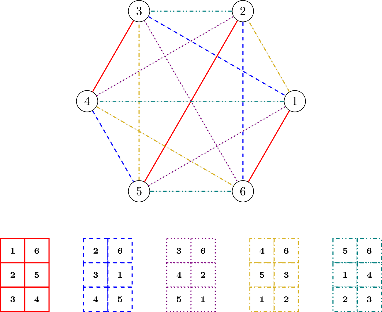
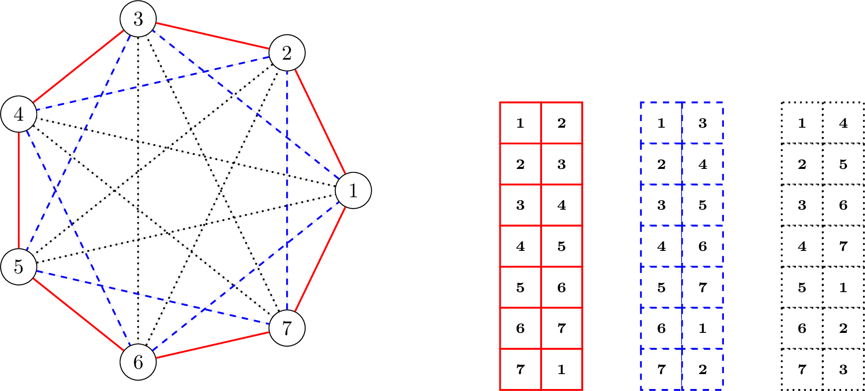
10.1.1 Statement and proof of Theorem 6↩︎
Theorem 6 (1-Equireplicate Partition for \(n\) Even). Let \(n\) be a positive even integer. Then there exists a \(1\)-equireplicate partition of \(\mathcal{B}_2\). One such construction of \(G_1,\ldots, G_{(n-1)}\) is as follows:
The subset \(G_g\), for \(g=1,\ldots, (n-1)\), consists of the pairs \((i,p_g(i))\) where \(i\in \{1,2,\ldots,n-1\}\) and \(p_g:\{1,\ldots, n-1\}\rightarrow \{1,\ldots, n\}\) is defined as follows: \[p_g(i)=\begin{cases}-i+2g\;\pmod{n-1},&i\neq g\pmod{n-1},\\ n,& i=g,\end{cases}\] where if \(-i+2g \pmod{n-1}=0\), we set the value to \(n-1\). Note that each pair \((i,j) \in \mathcal{B}_2\) is listed twice within its subset, except for \((g,n)\) which appears only once.
Proof. First, we establish some basic properties about the maps \(p_g\), \(g=1,\ldots, n-1\).
The map \(p'_g(i)=-i+2g \pmod{n-1}\) on \(\{1,2,\ldots, n-1\}\) is its own inverse: \[-(-i+2g)+2g\pmod{n-1}=i-2g+2g\pmod{n-1}=i\pmod{n-1}.\]
\(p'_g(i)\) has unique fixed point \(i=g\): Suppose that \(i=-i+2g\pod{n-1}\). This implies that \(2i=2g\pmod{n-1}\) and since \(n-1\) is odd this implies that \(i=g \pmod{n-1}\).
\(p'_g\) maps \(i\) to distinct values for different \(g\): Suppose to the contrary that \(-i+2g=-i+2g'\pmod{n-1}\). Then \(2g=2g'\pmod{n-1}\) and since \(n-1\) is odd, this implies that \(g=g'\pmod{n-1}\).
We see that each subset \(G_g\) contains \(n/2\) pairs, since \(p'_g(i)\) has \(n-1\) inputs, a unique fixed point, and is its own inverse. Furthermore, by construction each \(G_g\) contains exactly one pair with the value \(i\), since \(p'_g\) is its own inverse. By property (c) above, we have that \(G_g\) and \(G_g'\) are disjoint.
Since there are \(n-1\) disjoint subgroups, each with \(n/2\) pairs, and each pair occurs at most once, it follows that all \(n(n-1)/2\) pairs are accounted for. Thus, we have a \(1\)-equireplicate partition of \(\mathcal{B}_2\). ◻
10.1.2 Statement and proof of Theorem 7↩︎
Theorem 7 (2-Equireplicate Partition for \(n\) Odd). Let \(n\) be a positive odd integer. Then there exists a \(2\)-equireplicate partition of \(\mathcal{B}_2\). One such construction of \(G_1,\ldots, G_{(n-1)/2}\) is as follows:
For \(g=1,\ldots,(n-1)/2\), define \[G_g = \{\{i,j\}\in \mathcal{B}_2| (i-j)=\pm g\pmod{n}\}.\]
Proof. First we will establish the following claims:
Each \(i\) is paired to two distinct values within each \(G_g\): Note that for \(g\neq -g\; (\mod n)\), since \(g\neq 0 \pmod{n}\) and \(n\) is odd. Thus, \(i+g\) and \(i-g \pmod{n}\) are distinct.
No \(i\) is ever paired with itself in any \(G_g\): Suppose to the contrary that \(i\pm g=i \pmod{n}\). But then \(\pm g=0\pmod{n}\). However, this contradicts that \(g\in \{1,2,\ldots,(n-1)/2\}\) as none of these values are \(0\pmod{n}\).
No pair appears in two groups: Let \(g,g'\in \{1,2,\ldots, (n-1)/2\}\). Note that \(g\neq -g'\pmod{n}\), since \(-g'\pmod{n}\) is not a member of the set. Thus, if \(i-j=\pm g\pmod{n}\) and \(i-j=\pm g'\pmod{n}\), then the signs must be the same. Hence, \(g=g'\pmod{n}\).
We see that each \(G_g\) has \(n\) pairs, and is a \(2\)-equireplicate design. Since the \(G_g\)’s are disjoint, we have a \(2\)-equireplicate partition of \(\mathcal{B}_2\). ◻
10.1.3 Proof of Theorem 3↩︎
Proof. We start showing that the output of Algorithm 1 is an \(r\)-equireplicate design. Let \(p_g\) be as defined in Theorem 6. Evaluating at \(g+i\), we have: \[p_g(g+i)=\begin{cases} g-i\pmod{n-1}, & i\neq 0\pmod{n-1}\\ n, &i=0\pmod{n-1}. \end{cases}\] To avoid duplicates, we restrict \(i\in\{1,2,\ldots, n/2-1\}\). We see that Algorithm 1 produces the union of the first \(r\) subsets of the 1-equireplicate partition constructed in Theorem 6. Since the \(1\)-equireplicate partition consists of disjoint 1-equireplicate designs, the output of Algorithm 1 is an \(r\)-equireplicate design.
The output of Algorithm 2 is the union of the first \(r/2\) subsets of the \(2\)-equireplicate partition constructed in Theorem 7. By the same reasoning as in part 1, the result is an \(r\)-equireplicate design.
Both algorithms can be seen to have computational complexity \(O(nr)\) due to the nature of the nested for-loops.
Since the output \(D\) of both algorithms is an \(r\)-equireplicate design for \(k=2\), then by definition every \(1\)-subset of \(\{1,2, \ldots, n\}\) is contained in the same number \(r\) of pairs of \(D\). Thus \(D\) is a minimum variance design by Theorem 1 of [@lee1990u], page 195. Moreover, the variance of the incomplete U-statistics induced by \(D\) is \(\operatorname{Var} U_{n,D}^{(2)} =|D|^{-1} (2(r-1)\sigma_1^2 + \sigma_2^2)\) by Example 1 in [@lee1982incomplete]. ◻
Remark 10. An \(r\)-equireplicate partition can also be interpreted as an \(r\)-factorization of \(K^{(2)}_n\), which is the complete graph with \(n\) vertices. This construction decomposes \(K^{(2)}_n\) into \(r\)-regular spanning subgraphs, called \(r\)-factors, whose edge sets are \(r\)-equireplicate designs. In particular, when \(n\) is even, a \(1\)-factorization always exists and is equivalent to finding an edge coloring of \(K^{(2)}_n\) ([@bondy1976graph], ch.6). In Figure 7, we present the output of Algorithm 1 when \(n=6\) and \(r=5\) together with the corresponding edge coloring of \(K^{(2)}_6\). On the other hand, when \(n\) is odd, \(K^{(2)}_n\) cannot be decomposed into \(1\)-factors but a \(2\)-factorization always exists and is equivalent to finding disjoint cycles whose union forms \(K^{(2)}_n\) [@alspach2008wonderful]. In Figure 8, we present the output of Algorithm 2 for \(n=7\) and \(r=6\) together with the corresponding disjoint cycles decomposition of \(K^{(2)}_7\). In graph theory, the main interest is not only in designing algorithms to build either \(r\)-factorizations or \(r\)-factors, but in understanding under which conditions these exist and also how many non-isomorphic factorizations there are (see e.g., ch. 10 of [@wallis2016introduction] that discusses the number of possible \(1\)-factorizations of \(K^{(2)}_{2n}\)). Thus, our algorithms offer one efficient approach among many potential other ways to construct \(r\)-equireplicate designs. However, to the best of our knowledge, this is the first comprehensive and constructive treatment for \(k = 2\) in the literature of incomplete U-statistics based on deterministic designs.
10.2 Construction of r-equireplicate designs when k > 2↩︎
In principle, we can extend definition 2 to consider an \(r\)-equireplicate partition of \(\mathcal{B}_k\) and aim at building \(r\)-equireplicate designs by unioning the elements of either a \(1\)-equireplicate partition if \(k \mid n\) or of a \(k\)-equireplicate partition if \(k \nmid n\). However, when \(k \mid n\) and \(k>2\), even if the existence of a \(1\)-equireplicate partition is guaranteed by Baranyai’s theorem [@baranyai1975factorization], there is no known general sequential construction that would allow us to build an \(r\)-equireplicate design for any \(n\) and \(r \in \{1,\ldots,\binom{n-1}{k-1} \}\). Indeed, there exist only some efficient algorithmic constructions for \(k=3\) and \(k=4\) cases [@yan2022construction], but they impose additional divisibility conditions on \(n\). The situation becomes even more challenging when \(k \nmid n\). In this case, the problem is equivalent to constructing a \(k\)-factorization of the complete \(k\)-uniform hypergraph \(K_n^{(k)}\). However, even the existence of such a factorization is not guaranteed—let alone an efficient algorithm for its construction—as this remains an open problem in combinatorics (see e.g., [@bailey2010hamiltonian; @petecki2014cyclic] that discusses cyclic decompositions of \(K_n^{(k)}\)).
Remark 11 (Minimum Variance when \(k > 2\)). Even if constructing an \(r\)-equireplicate partition were both feasible and computationally efficient, when \(k > 2\) we no longer have the guarantee that the individual \(r\)-equireplicate designs forming the partition—or a fortiori, any union of them—achieve minimum variance. When \(k>2\), a sufficient condition for achieving minimum variance is that a design is both equireplicate and linear, as shown in Lemma 4. We have provided a novel interpretation of this specific class of designs within our equireplicate framework, enabling us to derive a closed-form expression for the variance of the corresponding incomplete U-statistic (see Lemma 4) as well as its Berry-Esseen bound, derived in Corollary 3, and asymptotic properties, derived in Corollary 4.
However, if we settle for a more attainable goal, we can still construct a \(r\)-equireplicate design in some settings, even when \(k>2\), via a partial equireplicate partition.
Definition 3. [Partial Equireplicate Partition] Let \(n\) and \(r\) be given. A collection \(G_1,\ldots, G_{q}\) of subsets of \(\mathcal{B}_k\) is a partial \(r\)-equireplicate partition if \(\bigcup_{g=1}^{q} G_g \subset \mathcal{B}_k\), the subsets are mutually disjoint and each subset \(G_g\) is an \(r\)-equireplicate design.
In the next theorem, we show that we can construct a partial \(k\)-equireplicate partition under some conditions on \(n\) and \(k\), and for any strictly increasing natural number valued sequence of choice. We denote with \(\mathcal{C}_n = \{ a \in \mathbb{Z}_n| \; \text{gcd}(a,n) = 1 \}\) the set of coprimes of \(n\) and with \(\phi(n) = \mid \mathcal{C}_n \mid\) its cardinality, which is known as Euler’s totient function.
Theorem 8 (Partial \(k\)-Equireplicate Partition). Let \(k > 2\) and \(\eta: \{0, \ldots, k-1\} \to \mathbb{N}_0\) be any strictly increasing natural number valued sequence. Take \(n\) to be a positive integer such that \(n > 3\;\eta(k-1)\;\{\eta(k-1) - \eta(0)\}\). Then there exists a partial \(k\)-equireplicate partition of \(\mathcal{B}_k\). One such construction is a collection of \(\phi(n)\) subsets \(G_1,\ldots, G_{q}\), where subset \(G_g\) for \(g \in \mathcal{C}_n\) is defined as:
\[G_{g}=\bigl\{ \,\{\,i+g\bigl[\eta(j)- \eta(0)\bigr]\pmod{n} \; | \; j\in \{0, \ldots, k-1\}\} \;| \; i\in\mathbb{Z}_{n} \bigr\}. \label{def:cyc95des}\tag{19}\]
10.2.1 Proof of Theorem 8↩︎
Proof. The construction of the partial partition relies on the map \(f: \mathbb{Z}_n \times \mathcal{C}_n \to D \subset \mathcal{B}_k\) which inputs a couple \((i,g)\) and outputs \(\{i+g\bigl[\eta(0)- \eta(0)\bigr], \ldots, i+g\bigl[\eta(k-1)-\eta(0)\bigr]\}\), which is an element of \(\mathcal{B}_k\). To avoid potential confusions, we will refer to a given element of \(G_g\) as a block. We now establish the following claims on the previously defined map:
The map \(f\) assigns to each couple \((i, g)\) an element of \(\mathcal{B}_k\).
First of all, consider \((i,g) = (0,1)\), which for sure belongs to \(\mathbb{Z}_n \times \mathcal{C}_n\). Since \(n > 3\;\eta(k-1)\;[\eta(k-1) - \eta(0)] > \eta(k-1)\) by assumption, the first block of \(G_{1}\), generated by \((i,g) = (0,1)\), contains \(k\) distinct elements. This also implies that all blocks of \(G_{1}\), generated by \((i,1)\), contain \(k\) distinct elements because shifting by the same \(i \in \mathbb{Z}_n \pmod{n}\) each element of a block of size \(k\), preserve the original distinction within the first block of \(G_1\). For a generic \(G_g\), consider that the first block of each \(G_g\), generated by \((0,g)\), has \(k\) distinct element since \(g \in \mathcal{C}_n\) just permutes the elements of the first block of \(G_1\) which are distinct, under \(n > \eta(k-1)\). To conclude the proof of this part, we just need to verify that for each \(g \in \mathcal{C}_n\), all the blocks of \(G_g\) contain \(k\) distinct elements. We have already shown that the first block of each \(G_g\) contains \(k\) distinct elements, but then all other blocks, generated by \((i,g)\) shifting by \(i \in \mathbb{Z}_n \pmod{n}\), will contain distinct elements for the same reasoning outlined at the beginning for \(G_1\).
The map \(f\) is injective and the subsets forming the partition are mutually disjoint.
We prove the injectivity of \(f\) by contradiction. Suppose \(f\) is not injective, then there exist distinct \((i_1,g_1)\) and \((i_2,g_2)\), meaning that \(i_1 = i_2\) and \(g_1 = g_2\) cannot occur at the same time, such that \(f(i_1,g_1) = f(i_2,g_2)\). We start by introducing a permutation \(\sigma:\{0, \ldots, k-1\} \to \{0, \ldots, k-1\}\), defined as a bijection from the set \(\{0, \ldots, k-1\}\) onto itself. If \(f(i_1,g_1) = f(i_2,g_2)\), then there must exist at least two distinct permutations \(\sigma\), since one is the identity that maps an index to itself, such that for all \(j \in \{0, \ldots k-1\}\):
\[i_1 + g_1 [\eta(j) - \eta(0)] \equiv i_2 + g_2 [\eta(\sigma(j)) - \eta(0)] \pmod{n} \;.\label{eq:set95perm}\tag{20}\]
The key argument behind the proof, is to notice that if two blocks are equal in our \(D\), then all possible subsets of these two blocks of any given size must be equal as well. Thus, we consider the three distinct indices \(j,i, l \in \{0,,\ldots,k-1\}\) and solve the related system of \(\binom{k}{3}\) congruences:
\[\left\{ \begin{align} & i_1 + g_1 [\eta(j) - \eta(0)] \equiv i_2 + g_2 [\eta(\sigma(j)) - \eta(0)] \pmod{n} \\ & i_1 + g_1 [\eta(i) - \eta(0)] \equiv i_2 + g_2 [\eta(\sigma(i)) - \eta(0)] \pmod{n}\\ & i_1 + g_1 [\eta(l) - \eta(0)] \equiv i_2 + g_2 [\eta(\sigma(l)) - \eta(0)] \pmod{n} \end{align} \right.\]
\[\left\{ \begin{align} & i_1 - i_2 \equiv g_2 [\eta(\sigma(j)) - \eta(0)] - g_1 [\eta(j) - \eta(0)] \pmod{n} \\ & i_1 - i_2 \equiv g_2 [\eta(\sigma(i)) - \eta(0)] - g_1 [\eta(i) - \eta(0)] \pmod{n}\\ & i_1 - i_2 \equiv g_2 [\eta(\sigma(l)) - \eta(0)] - g_1 [\eta(l) - \eta(0)] \pmod{n} \end{align} \right.\]
Now we take the collections of congruences indexed first by \(i\) and then by \(l\) and subtract them from the collection indexed by \(j\) obtaining
\[\left\{ \begin{align} & g_2 [\eta(\sigma(j)) - \eta(\sigma(i))] - g_1 [\eta(j) - \eta(i)] \equiv 0 \pmod{n} \\ & g_2 [\eta(\sigma(j)) - \eta(\sigma(l))] - g_1 [\eta(j) - \eta(l)] \equiv 0 \pmod{n} \end{align} \right.\]
We now multiply both collections of congruences to match the \(g_1\) terms and subtract them to finally obtain \[g_2\{ [\eta(\sigma(j)) - \eta(\sigma(i))] [\eta(j) - \eta(l)] - [\eta(\sigma(j)) - \eta(\sigma(l))] [\eta(j) - \eta(i)] \} \equiv 0 \pmod{n}.\]
Since \(g_2 \in \mathcal{C}_n\), we can divide both sides of the congruence by \(g_2\) and obtain \[[\eta(\sigma(j)) - \eta(\sigma(i))] [\eta(j) - \eta(l)] - [\eta(\sigma(j)) - \eta(\sigma(l))] [\eta(j) - \eta(i)] \equiv 0 \pmod{n}. \label{eq:inj95equiv}\tag{21}\] Now we show that that the absolute value of (21 ) is bounded above by the quantity \(3\;\eta(k-1)\;[\eta(k-1) - \eta(0)]\). We start by noticing that the LHS of (21 ) can be developed to obtain
\[\text{LHS} = \eta(\sigma(i))\left[\eta(l)-\eta(j)\right]+\eta(\sigma(j))\left[\eta(i)- \eta(l)\right]+\eta(\sigma(l))\left[\eta(j)-\eta(i)\right] .\]
Since the sequence is strictly increasing, we know that for any \(u,v \in \{0,\ldots, k-1\}\), \(\left| \eta(u)-\eta(v)\right| \leq [\eta(k-1) - \eta(0)]\). But then, for the triangle inequality and Cauchy-Schwarz \[\begin{align} & \left| \text{LHS} \right| & < & \left|\eta(\sigma(i))\right|\left|\eta(l)-\eta(j)\right|+\left|\eta(\sigma(j))\right|\left|\eta(i)-\eta(l)\right|+\left|\eta(\sigma(l))\right|\left|\eta(j)-\eta(i)\right| \\ & & < & \;\eta(k-1) [\eta(k-1) - \eta(0)] + \eta(k-1) [\eta(k-1) - \eta(0)] + \eta(k-1) [\eta(k-1) - \eta(0)]\\ & & = & \;3\;\eta(k-1)\;[\eta(k-1) - \eta(0)]. \end{align}\] Since \(n > 3\;\eta(k-1)\;[\eta(k-1) - \eta(0)]\) by assumption, this implies that all the possible solutions of (21 ) must verify \[[\eta(\sigma(j)) - \eta(\sigma(i))] \;[\eta(j) - \eta(l)] = [\eta(\sigma(j)) - \eta(\sigma(l))] \;[\eta(j) - \eta(i)] .\]
However, the only possible solution is when \(j=\sigma(j)\), \(i=\sigma(i)\) and \(l=\sigma(l)\). This because both the three indices \(j\),\(i\) and \(l\) and their permutations are distinct among themselves, and the sequence is strictly increasing. But this contradicts our original statement on the existence of at least two distinct permutations that guarantee (20 ). Thus the map \(f\) is injective. This results implies a fortiori that \(G_a \cap G_b = \varnothing\) for all distinct \(a,b \in \mathcal{C}_n\) meaning that the subsets forming the partition must be mutually disjoint.
The set of images \(D \subset \mathcal{B}_k\) thus \(f\) is not surjective.
This is a requirement of definition 3 to obtain a partial equireplicate partition. Consider that \(|\mathcal{B}_k| = \binom{n}{k}\). But since the map is injective under our assumptions, we know that \(|D| = n \; \phi(n)\), which achieves its maximum when \(n\) is prime. Thus, if we have that \(n \; (n-1) < \binom{n}{k}\) this ensures that \(D = \bigcup_{g=1}^{q} G_g \subset \mathcal{B}_k\). Under our assumptions that \(k > 2\) and \(n > 3\;\eta(k-1)\;[\eta(k-1) - \eta(0)]\), \(n \; (n-1) < \binom{n}{k}\) thus \(f\) is not surjective.
Each \(G_g\) for \(g \in \mathcal{C}_n\) is a \(k\)-equireplicate design.
This last point is easy to show since it comes automatically when using cyclic constructions (see [@lee1990u], starting from page 198, for a detailed explanation). Indeed, we have that \(G_1 = \{i+\bigl[\eta(0)- \eta(0)\bigr], \ldots, i+\bigl[\eta(k-1)- \eta(0)\bigr]\}\) and since we have shown that all \(n\) elements are distinct, and we know that \(i \in \mathbb{Z}_n\), then each element of \(\mathbb{Z}_n\) will appear exactly \(k\) times. The same holds as well for a generic \(G_g\) because we have shown that also all his elements are distinct at the start.
Since we have verified all our claims, then our proposed construction is a partial \(k\)-equireplicate partition. ◻
10.2.2 Proof of Theorem 4↩︎
Proof. For a given value of \(g \in \mathcal{C}_{n,r}\), Algorithm 3 builds the subset \(G_g\), as defined in Theorem 8 where each \(G_g\) is a \(k\)-equireplicate design. As already underlined for the \(k=2\) case, see the proof of Theorem 3, if \(G_1,\ldots, G_{q}\) is a partial \(t\)-equireplicate partition, then the union of any \(s\) of the subsets yields a \(st\)-equireplicate design. In our case, the output of Algorithm 3 is the union of the first \(r/k\) subsets of the partial \(k\)-equireplicate partition constructed in Theorem 8. Thus, by the previous reasoning with \(t=k\) and \(s=r/k\), it follows that the output of Algorithm 3 is an \(r\)-equireplicate design. Regarding the computational complexity, we start by noticing that building \(\mathcal{C}_{n,r} = \{a \in \{1,\ldots, r/k \}| \; \text{gcd}(a,n) = 1 \}\) requires \(O(r/k \log(n))\) using the standard Euclidean algorithm. Then, there are three nested for-loops with total computational complexity \(O(nr)\), since the first loop concerns \(r/k\) iterations, the second \(n\) and the third \(k\). Therefore, asymptotically Algorithm 3 runs in \(O(nr)\). ◻
11 Numerical Experiments↩︎
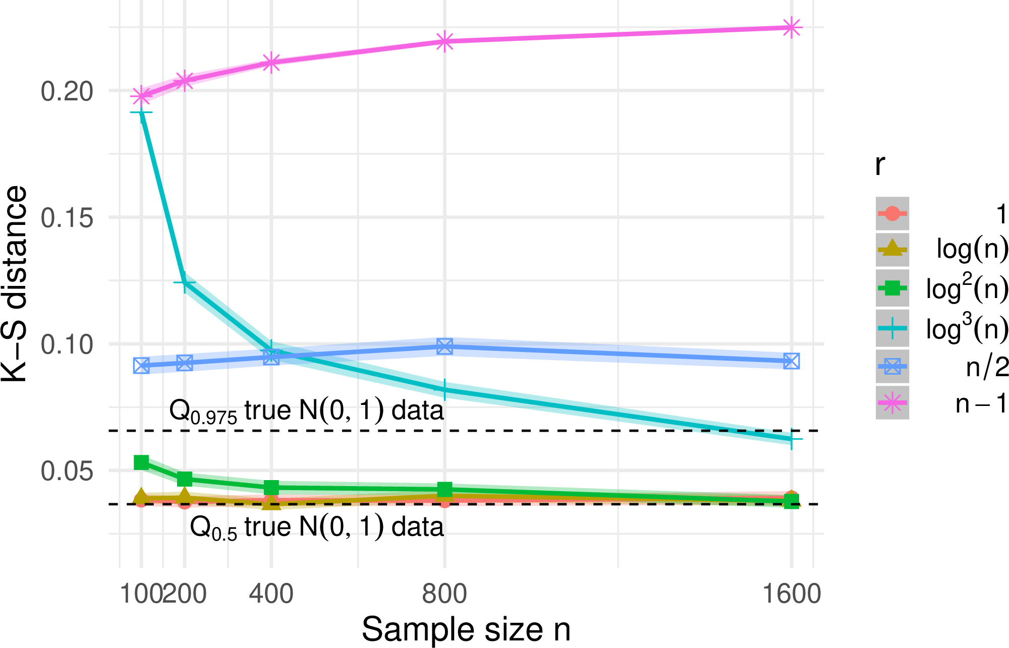
In 8.3, we discuss an analog of Observation 1 that applies specifically to equireplicate designs and \(k\)-uniform, \(r\)-regular hypergraphs.↩︎
If \(k \nmid n\), \(D^{\perp}_n\) would be of size \(\lfloor n\rfloor/k\) where \(\lfloor n\rfloor\) is the largest integer, smaller than \(n\), such that \(k \mid \lfloor n\rfloor\). To avoid unnecessary complications, we restrict ourselves to the case \(k \mid n\) in the main text.↩︎
Note that, as expected, when \(r=n-1\) the KS CI indicate a clear departure from normality. This occurs because we recover the complete uMMD, which under the null is non-Gaussian.↩︎
Note that \(r\) must be a multiple of \(k=4\). If it is not the case, we select the nearest multiple. Moreover, when \(r=1\), we use the design \(D_n^{\perp}\), described in Proposition 2.↩︎