Survival of the fittest Cox model: Pivotal variable selection for time-to-event data
October 22, 2025
Abstract
We revisit Cox’s proportional hazards model to improve variable selection in survival analysis. A square-root transformation of the partial likelihood renders the selection of the regularization parameter pivotal, free of the unknown baseline hazard and censoring mechanism. The resulting criterion borrows from information criteria such as BIC and from penalized regression methods such as the lasso, taking the best of both. On simulated and real data, our method substantially improves upon state-of-the-art approaches used daily in support recovery.
Keywords: Cox model; Model selection; Pivotal detection boundary; Pivotal information criterion.
1 Introduction↩︎
1.1 Setting↩︎
We consider the classical survival analysis setting. Survival analysis is concerned with the study of time-to-event data and censoring information. Such data arise in many fields, for example in medicine, where the event of interest may be the death of a patient, or in engineering, where the survival time may represent the lifetime of a machine component. At the time of analysis, the event of interest may not yet have been observed for every individual, a phenomenon known as censoring. In addition to event times and censoring indicators, survival studies often collect covariates that can influence the outcome. In a clinical oncology trial, for example, variables such as tumour stage, patient age, smoking status, or gene expression may have a substantial impact on survival. Identifying the most relevant covariates improves the interpretability of the model, reduces overfitting, and facilitates the detection of meaningful prognostic and predictive factors that can support clinical decision-making.
Formally, survival analysis assumes that two random variables underlie the data: the event time \(T\) and the censoring time \(C\). Let \((T_1, C_1), \dots, (T_n, C_n)\) be an independent sample from the joint distribution of \((T, C)\). The observed right-censored data consist of triplets \((y_i, \delta_i, {\boldsymbol{x}}_i)_{i=1,\ldots,n}\) where \(y_i=\min(t_i, c_i)\), \(\delta_i=I\{t_i\leq c_i\}\) and \({\boldsymbol{x}}_i\in{\mathbb{R}}^p\) denotes the vector of covariates for the \(i\)th individual. We consider the non-informative censoring setting that \(T_i\) and \(C_i\) are conditionally independent given \({\boldsymbol{x}}_i\). We denote by \(X\in \mathbb{R}^{n\times p}\), \({\boldsymbol{y}}\in \mathbb{R}^n\) and \({\boldsymbol{\delta}}\in \mathbb{R}^n\) the vectorized form of the data. Let \(\tau\) be the end of study time.
The primary objective is to characterize the distribution of the event time \(T\). A common quantity of interest is the survival function \(S(t\vert\mathbf{x}) := {\mathbb{P}}(T>t\vert\mathbf{x})\) which gives the probability that an individual with covariates \(\mathbf{x}\) survives beyond time \(t\) and is commonly used for graphical representations. For model specification, however, it is often more convenient to work with the hazard function \[h(t\vert\mathbf{x}):=\frac{f(t\vert\mathbf{x})}{S(t\vert\mathbf{x})}=\lim_{\Delta t\to 0}\frac{1}{\Delta t}{\mathbb{P}}\left(t\leq T<t+\Delta t\,\vert\,T\geq t,\,\mathbf{x}\right)\] which describes the instantaneous risk of experiencing the event at time \(t\), given survival up to that time. Here \(f(t\vert\mathbf{x})\) denotes the conditional density of \(T\). While the survival function captures the long-term probability of survival, the hazard function captures the instantaneous failure rate. The two are tightly connected through \[S(t\vert\mathbf{x})=\exp{\left(-\int_0^t h(u\vert\mathbf{x})\mathrm{d}u\right)}=:\exp\{-H(t\vert\mathbf{x})\}.\]
1.2 The Cox model and Cox’s partial likelihood↩︎
The proportional hazards model for survival data, also known as the Cox model [1], assumes that the hazard at time \(t\) depends on the covariates through \[h(t\vert{\boldsymbol{x}})=h_0(t)\exp{({\boldsymbol{x}}^{ \mathrm{\scriptscriptstyle T} }\boldsymbol{\beta})},\] where \(h_0\) is the unknown baseline hazard function and \(\boldsymbol{\beta}\in\mathbb{R}^p\) is the regression coefficient vector. The associated linear predictor \(\mu_{\boldsymbol{\beta}}(\mathbf{x})={\boldsymbol{x}}^{ \mathrm{\scriptscriptstyle T} }{{\boldsymbol{\beta}}}=\sum_{j=1}^p \beta_j x_j\) has no intercept to avoid a non-identifiability issue with the baseline hazard function \(h_0\). Cox showed that the estimation of \(\boldsymbol{\beta}\) can be separated from that of \(h_0(t)\) by introducing the partial likelihood. Assuming, for simplicity, that there are no ties among the observed times \(y_1,\dots,y_n\), and under the assumption that censoring is independent of the covariates, the log-partial likelihood of the observed data is \[\label{eq:partiallik} l^{\rm partial}(\boldsymbol{\beta}; X, \mathbf{y}, \boldsymbol{\delta}) = \sum_{i=1}^n \delta_i \left[ \mu_{\boldsymbol{\beta}}(\mathbf{x}_i) - \log\left(\sum_{j: y_j \geq y_i} \exp\{\mu_{\boldsymbol{\beta}}(\mathbf{x}_j)\}\right)\right],\tag{1}\] where the outer sum is taken only over individuals who experienced the event (\(\delta_i=1\)), and the inner sum ranges over the risk set at time \(y_i\), i.e., all subjects still under observation just prior to \(y_i\). Unlike the full likelihood, the partial likelihood does not depend on \(h_0(t)\) and can be maximized directly with respect to \(\boldsymbol{\beta}\). It is, in fact, a profile likelihood [2].
1.3 Model selection for survival analysis↩︎
The linearity of \(\mu_{\boldsymbol{\beta}}\) in Cox’s model is convenient for at least three reasons. First, the negative log-partial likelihood function is convex and so easy to optimize. Second, the linear model can be interpreted as it captures the linear main effects in each input. Third, the set of influential inputs \[\label{eq:S} {\cal S}:=\left\{j\in\{1,\ldots,p\} : x_jhas an impact on survival\right\}\tag{2}\] corresponds to the indices of entries of \({\boldsymbol{\beta}}\) different from zero: \({\cal S}\equiv\left\{j\in\{1,\ldots,p\} : \beta_j\neq 0\right\}\).
The search of \(\cal S\) is a central objective in survival analysis and constitutes the main focus of this paper. From a practical standpoint, determining which covariates \({\cal S}\) significantly influence the risk of death is crucial for scientific and medical applications. In modern high-dimensional datasets such as genomic or imaging data, the number of potential covariates is often large and careful variable selection becomes crucial. We review three different approaches used in survival analysis to estimate \({\cal S}\).
The first approach fits the full Cox model by maximizing the partial likelihood 1 , and tests each coefficient against \(H_0:\boldsymbol{\beta}_j=0\). The resulting per-covariate p-values are then adjusted with the Benjamini–Hochberg procedure [3] to control the false discovery rate at a prescribed level, and the selected set collects the covariates whose adjusted p-value falls below that level. This procedure inherits the asymptotics of the maximum partial-likelihood estimator and is therefore reliable only when \(n\gg p\). When \(p\) is comparable to or larger than \(n\), the estimator becomes unstable or undefined, the p-values are no longer trustworthy, and the nominal control of the false discovery rate is lost, precisely the regime arising in modern applications.
A second approach enforces sparsity on \(\hat{\boldsymbol{\beta}}\) by maximizing 1 over subsets of the covariates and selecting the size of the optimal subset with an information criterion such as AIC [4], [5] or BIC [6], namely minimizing \[\operatorname{BIC} = 2l_n\left(\boldsymbol{\beta}; X,\mathbf{y}, \boldsymbol{\delta}\right)+\lambda C(\boldsymbol{\beta}),\] where \(l_n=-l^{\rm partial}/n\) and the complexity measure \(C(\boldsymbol{\beta})=\#\left\{\beta_j\neq 0,\, j=1,\ldots,p\right\}\) counts the covariates used in the model. For censored survival data, the relevant sample size is not the number \(n\) of subjects but the number \(d=\sum_{i=1}^n \delta_i\) of uncensored observations (observed events). Hence, the BIC penalty is taken as \(\lambda = \log d\) rather than \(\log n\) [7] (\(\lambda=2\) for AIC). This penalty is derived from an asymptotic approximation of Bayes factors and is designed neither to control the familywise error rate nor the false discovery rate. Moreover, evaluating all \(2^p\) candidate subsets is computationally prohibitive in high dimensions, so one usually relies on greedy forward selection instead.
A third approach is the lasso [8], [9], which restores tractability by convexifying the criterion: the discrete complexity measure is replaced by the convex \(\ell_1\) penalty \(C(\boldsymbol{\beta})=\|\boldsymbol{\beta}\|_1\) turning subset selection into the convex optimization problem \[\hat{\boldsymbol{\beta}}(\lambda)=\arg\min_{\boldsymbol{\beta}}l_n\!\left(\boldsymbol{\beta}; X, \mathbf{y},\boldsymbol{\delta}\right)+\lambda\|\boldsymbol{\beta}\|_1.\] The \(\ell_1\) penalty shrinks coefficients and sets many of them exactly to zero, so a single fit yields a sparse estimate \(\hat{\mathcal{S}}\) and the whole solution path is computable even when \(p\gg n\). The regularization level \(\lambda\), which governs the size of the selected set, is typically chosen by cross-validation to optimize predictive performance. This choice targets prediction rather than support recovery, however, and provides no probabilistic control on the selected covariates: the cross-validated lasso is known to over-select.
To address these limitations, [10] introduced the Pivotal Information Criterion (PIC), a general framework that borrows from information criteria such as BIC and from penalized regression methods such as the lasso, taking the best of both. Like the latter, it relies on a continuous sparsity-inducing penalty; like the former, its regularization level is fixed a priori rather than estimated from the data. Specifically, PIC provides a probabilistic choice of \(\lambda\) under the null hypothesis \(H_0:\boldsymbol{\beta}=\mathbf{0}\) and thereby controls the false discovery rate under the null while retaining a high probability of recovering \(\mathcal{S}\), as established for regression and classification tasks [10], [11]. Our goal here is to improve model selection in survival analysis by properly deriving PIC.
2 PIC for Cox’s model↩︎
Inspired by the universal threshold [12], theoretical results on thresholding estimators [13], the quantile universal threshold [14] and square-root lasso [15], the Pivotal Information Criterion (adapted to our setting) is defined as \[\label{eq:PIC} {\rm PIC}=\phi\!\left[l_n\!\left(\boldsymbol{\beta}; X, \mathbf{y}, \boldsymbol{\delta}\right)\right] +\lambda C(\boldsymbol{\beta}),\tag{3}\] where \(l_n\) is a loss function (typically the negative log-likelihood normalized by the sample size \(n\)), \(\phi\) is a univariate function, and \(C\in\mathcal{C}_{\ell_1}\) is a model complexity measure drawn from the class of first-order \(\ell_1\)-equivalent penalties on which the PIC framework is built; we recall this class in Definition 1. PIC selects its regularization parameter \(\lambda\) so that two properties hold: the calibrating quantity is asymptotically pivotal (in that its limiting distribution does not depend on unknown nuisance parameters) and \(\lambda\) is set at the detection boundary (the smallest penalty that screens out all noise covariates under \(H_0\) with high probability \(1-\alpha\) for a prescribed small \(\alpha\)). Because of these two properties, we refer to this parameter as \(\lambda_\alpha^{\rm PDB}\), for pivotal detection boundary. The transformation \(\phi\), if it exists, is crucial to enable the construction of such a value \(\lambda\).
We recall from [10] the class of complexity measures underlying 3 .
Definition 1. Let \(\rho:{\mathbb{R}}\to[0,\infty)\) be even and nondecreasing on \({\mathbb{R}}^+\). For \(\boldsymbol{\beta}\in\mathbb{R}^p\), define \(C(\boldsymbol{\beta})=\sum_{i=1}^p\rho(\beta_i)\). We say that \(C\in\mathcal{C}_{\ell_1}\) is a first-order \(\ell_1\)-equivalent complexity measure if \(\lim_{\epsilon\to0^+}\frac{C(\epsilon\boldsymbol{\beta})}{\epsilon}=\|\boldsymbol{\beta}\|_1\).
The class contains the convex \(\ell_1\) penalty of the lasso, as well as the most commonly used nonconvex penalties, including SCAD [16] and MCP [17]. The statistical advantage of a nonconvex \(C\in\mathcal{C}_{\ell_1}\) is that it shrinks the estimated nonzero coefficients less aggressively towards zero, thereby improving the estimation of the influential covariates \({\cal S}\).
Before specifying in the following theorem the choice of \((\phi,\,l_n)\) that yields the pivotal criterion for survival analysis, we state its conditions.
Assumption 1. With \(\tau\) the end-of-study time, \({\mathbb{P}}(T_i\le\tau)=1\), the baseline hazard \(h_0\) is bounded on \([0,\tau]\), and \({\mathbb{P}}(y_i\ge\tau)\ge k_\tau>0\) for some constant \(k_\tau>0\).
Assumption 2. The vectors of variables \(\mathbf{x}_1, \ldots, \mathbf{x}_n \in \mathbb{R}^p\) in \(X\) are fixed, uniformly bounded \(\left|x_{i j}\right| \leq B_n\), and centred \(\sum_{i=1}^n \mathbf{x}_i=\mathbf{0}\).
Assumption 3. The number of variables \(p\) is allowed to tend to infinity with \(n\) such that \(B_n^4(\log (p n))^7= O\left(n^{1-c}\right)\) for some \(c>0\).
Theorem 1. Consider the pivotal information criterion 3 with the square-root transform \(\phi(u)=u^{1/2}\), Cox’s minus-log-partial likelihood \(l_n=-l^{\rm partial}/n\) for loss and complexity measure \(C\in\mathcal{C}_{\ell_1}\). Then:
The smallest \(\lambda\) for which \(\hat{\boldsymbol{\beta}}=\mathbf{0}\) is a local minimizer of 3 is the zero-thresholding function \[\label{eq:lambda0} \lambda_0(X, \mathbf{y}, \boldsymbol{\delta})=\frac{\left\|\nabla_{\boldsymbol{\beta}}l_n\left(\boldsymbol{\beta}; X, \mathbf{y},\boldsymbol{\delta}\right)\big|_{\boldsymbol{\beta}=\mathbf{0}}\right\|_\infty}{2\{l_n\left(\boldsymbol{0}; X, \mathbf{y},\boldsymbol{\delta}\right)\}^{1/2}}.\qquad{(1)}\]
Under \(H_0:\boldsymbol{\beta}=\mathbf{0}\) and assumptions 1–3, the distribution of \(\Lambda=\lambda_0(X,\mathbf{Y}_0,\boldsymbol{\Delta}_0)\), where \(\mathbf{Y}_0\) and \(\boldsymbol{\Delta}_0\) are random variables of the survival times and censoring indicators under \(H_0\), is asymptotically pivotal: its limiting law depends on the design \(X\) only through \(\Sigma_X=X^{ \mathrm{\scriptscriptstyle T} }X/n\) and is free of the baseline hazard \(h_0\) and the censoring mechanism behind \(\mathbf{Y}_0\) and \(\boldsymbol{\Delta}_0\).
Appendix 5 provides a proof. Part (ii) follows from a Gaussian approximation of the numerator of ?? combined with a law-of-large-numbers argument for its denominator; the unknown censoring probability \(p_0\) appears in both terms and cancels in the ratio, leaving a limit that depends on \(X\) only through \(\Sigma_X\). For any prescribed \(\alpha\in(0,1)\), the upper \(\alpha\)-quantile \(\lambda_\alpha^{\rm PDB}=F_\Lambda^{-1}(1-\alpha)\) is therefore a pivotal detection boundary: it is the smallest penalty level that screens out all noise covariates under \(H_0\) with probability at least \(1-\alpha\), without requiring estimation of any nuisance parameter. Plugging \(\lambda_\alpha^{\rm PDB}\) into 3 yields the PIC-Cox estimator \[\label{eq:pic95cox} \hat{\boldsymbol{\beta}}=\arg\min_{\boldsymbol{\beta}\in\mathbb{R}^p}\; \left\{\sum_{i=1}^n \delta_i \left[ \mu_{\boldsymbol{\beta}}(\mathbf{x}_i) - \log\left(\sum_{j: y_j \geq y_i} \exp\{\mu_{\boldsymbol{\beta}}(\mathbf{x}_j)\}\right)\right]\right\}^{1/2} +\lambda_\alpha^{\rm PDB}\,C(\boldsymbol{\beta}).\tag{4}\]
In practice the design \(X\) is fixed and \(\lambda_\alpha^{\rm PDB}\) is estimated by Monte Carlo: at each of \(M\) iterations we draw a null sample, evaluate the statistic \(\Lambda\) of ?? , and report the empirical \((1-\alpha)\)-quantile of the \(M\) draws. A natural way to generate the null data would be to bootstrap the observed times and censoring indicators \((\mathbf{y},\boldsymbol{\delta})\). Doing so, however, reshuffles the event times at every iteration and forces an \(O(np)\) reordering of the rows of \(X\) to rebuild the risk sets, which quickly dominates the cost. We avoid it entirely: as detailed in Appendix 6, expanding the risk-set averages in the gradient ?? and exchanging the order of summation rewrites its numerator as \[\big\|X^{ \mathrm{\scriptscriptstyle T} }\mathbf{u}\big\|_\infty, \qquad u_{\pi(i)}=e_i-\sum_{j\ge i}\frac{e_j}{r_j},\] where \(e_i\stackrel{\text{iid}}{\sim}\mathrm{Bernoulli}(1/2)\), \(\pi\) is a uniform random permutation, and \(r_i\) is the size of the risk set at the \(i\)th ordered time (which one may assume to be \(n-i+1\)). The permutation thus acts on the length-\(n\) vector \(\mathbf{u}\) rather than on \(X\), which is never reordered nor copied. Each draw only generates \(\mathbf{e}\) and \(\pi\), while the denominator \(2\big(n\sum_i e_i\log r_i\big)^{1/2}\) is obtained for all \(M\) draws at once by a single matrix product.
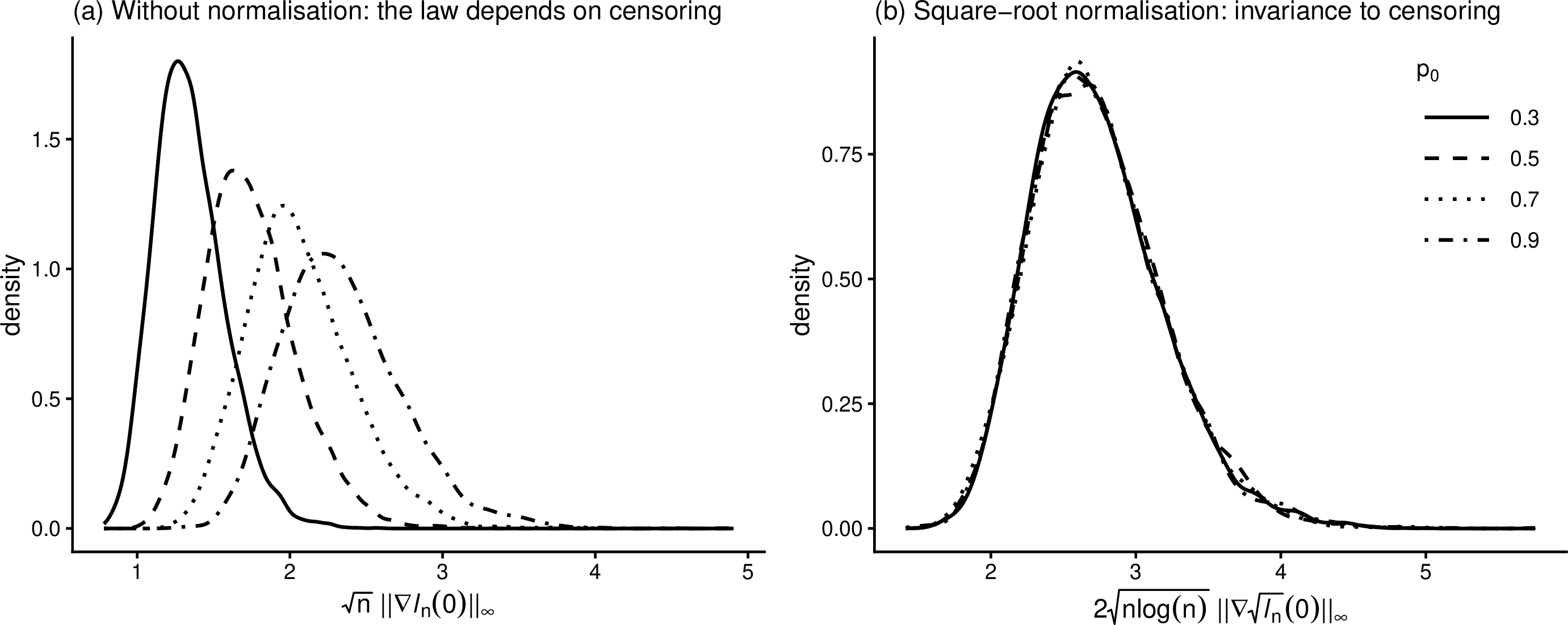
Figure 1 illustrates this pivotality on simulated null data, for a fixed design \(X\in\mathbb{R}^{200\times 50}\) and \(M=5000\) Monte Carlo replicates drawn under \(H_0\) at four censoring levels, \(p_0\in\{0.3,0.5,0.7,0.9\}\). The left panel reports the sup-norm of the bare gradient: it is clear that its statistic depends on \(p_0\) and is therefore not pivotal. The right panel reports the same quantity after the square-root normalization: the four densities now collapse onto a single curve.
3 Simulation studies and applications↩︎
3.1 Setup and baselines↩︎
We call PIC-lasso our estimator employing the lasso (i.e., convex \(\ell_1\)) penalty complexity measure \(C\) and PIC-scad its nonconvex analogue. We recommend
the latter, and consider here the former for quantifying the improvement in using a nonconvex model complexity measure \(C\). The pivotal detection boundary \(\lambda_\alpha^{\rm PDB}\) is
computed as described in Section 2 using significance level \(\alpha=0.05\) and \(2000\) Monte Carlo replications. Our method is compared against the
three established baselines discussed in Section 1.3. We recall the three baselines briefly. The first, denoted Cox+BH, fits the full Cox model and adjusts the obtained p-values by the
Benjamini-Hochberg method [3], selecting the covariates whose adjusted p-value falls below \(\alpha=0.05\). The second, denoted BIC, performs greedy forward selection with the BICpenalty \(\lambda=\log d\) on the number \(d\) of uncensored
observations rather than the total sample size \(n\), which has been shown to yield more reliable results [7]. The third, cv.glmnet, is the cross-validated lasso of [9] with the penalty
parameter \(\lambda\) selected by 10-fold cross-validation using partial-likelihood deviance, retaining the value \(\lambda_{\min}\) that minimizes this criterion.
3.2 Evaluation of the method by phase transition↩︎
We compare the different methods on simulated data through the prism of a phase transition in the probability of exact support recovery \({\rm PESR}={{\mathbb{P}}}(\hat{\cal S}={\cal S})\) as a function of the sparsity level \(s=|{\cal S}|\). This concept, originally studied by [18] and [19] for compressed sensing, describes a sharp transition: the probability of retrieving \({\cal S}\) is high when \(s\) is low, and suddenly drops to zero when \(s\) gets large. The longer \({\rm PESR}\) remains near one for larger \(s\), the better the detection method. Looking at the true positive rate \(\operatorname{TPR}:=\mathbb{E}(|\hat{\cal S}\cap\cal S|/|\cal S|)\) and the false discovery rate \(\operatorname{FDR}:=\mathbb{E}(|\hat{\cal S}\cap\bar{\cal S}|/|\hat{\cal S}|)\) also helps understand the reason why exact support recovery fails.
To estimate the different performance metrics, we perform \(300\) independent simulation runs for each sparsity level \(s\) given a fixed standardized Gaussian design \(X\in\mathbb{R}^{n\times p}\) with independent \(\mathcal{N}(0,1)\) entries. We deliberately work with an independent Gaussian design as correlation among predictors can only make exact support recovery harder, lowering the \({\rm PESR}\) of every method. A procedure that already fails in this most favourable setting cannot be expected to do better under correlation.
For a target support size \(s\) ranging from \(0\) upward, we draw a coefficient vector \(\boldsymbol{\beta}_s\) with exactly \(s\) nonzero entries, each equal to a \(\mathcal{U}(1,3)\) magnitude with a random sign and a uniformly chosen location. Following [20], the survival times are generated from an exponential Cox model with baseline hazard \(h_0=0.1\): \[T_i=\frac{-\log U_i}{h_0\,\exp(\mathbf{x}_i^{ \mathrm{\scriptscriptstyle T} }\boldsymbol{\beta}_s)},\qquad U_i\sim\mathcal{U}(0,1).\] Finally, censoring times are generated independently from an exponential distribution parameter chosen so as to achieve a target average censoring rate of approximately \(30\%\).
We report two regimes: a high-dimensional one with \(n=p=100\), where \(d\approx 70<p\) and the full Cox model is ill-posed, and a classical one with \(n=250\), \(p=50\), where \(d\approx 175>p\). In the former, Cox+BH is not defined hence omitted. Figure 2 presents the results.
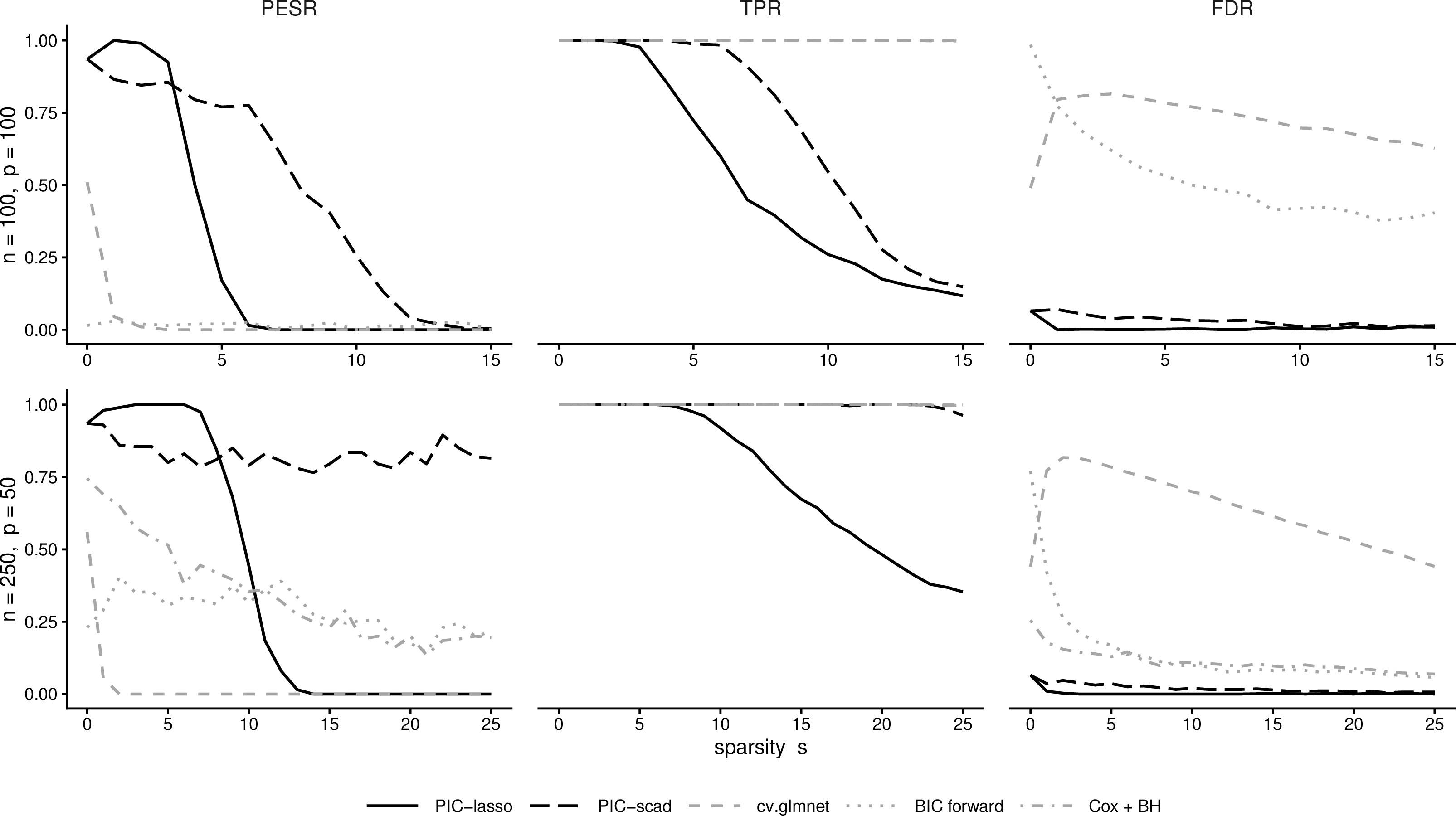
Figure 2: Phase transition of support recovery as a function of the true sparsity \(s\), averaged over \(M=300\) Monte Carlo replicates. Columns report the probability of
exact support recovery (PESR), the true positive rate (TPR), and the false discovery rate (FDR); rows correspond to the high-dimensional regime (\(n=100\), \(p=100\)) and the low-dimensional
regime (\(n=250\), \(p=50\)). In the high-dimensional regime Cox+BH is omitted..
We first examine the null case \(s=0\), which reveals how each method controls false discoveries when no signal is present. Both PIC variants achieve a false discovery rate of close to the nominal level \(\alpha=0.05\). By contrast, cv.glmnet has a false discovery rate of \(0.44\) when \(n=250\) and \(0.49\) when \(n=100\): it spuriously selects about half the covariates even when none is significant. BIC forward selection is even worse, with a higher false discovery rate in both regimes, saturating the model with noise
covariates. Among the competing baselines, Cox+BH keeps the false discovery rate closest to zero.
As the sparsity \(s\) increases, cv.glmnet maintains a true positive rate near one throughout, but its false discovery rate remains very high at every sparsity level, so that its exact-recovery probability
collapses to zero almost immediately in both regimes. BIC forward selection fares somewhat better in the low-dimensional regime, where its false discovery rate settles around \(0.07\)–\(0.13\) and its probability of exact support recovery stabilizes near \(0.25\)–\(0.35\); in the high-dimensional regime, however, its false discovery rate stays
above \(0.4\) and, as expected, its probability of exact support recovery never exceeds \(0.03\). Cox+BH achieves a moderate false discovery rate of about \(0.10\) in the low-dimensional setting and a probability of exact support recovery of \(0.4\)–\(0.7\) for small \(s\); when \(n=p=100\), however, the full Cox model is not identifiable and the procedure selects no covariate at all (\(\operatorname{TPR}=0\)).
The two PIC methods behave qualitatively differently from all three baselines. Their false discovery rate stays essentially at zero across the whole sparsity range in both settings. In the low-dimensional setting, PIC-lasso achieves perfect
exact support recovery (\({\rm PESR}=1\)) while the signal is sparse before dropping to zero past a critical sparsity: the phase transition. Throughout this regime PIC-scad consistently outperforms
PIC-lasso: at equal (near-zero) false discovery rate, the nonconvex measure mitigates the shrinkage bias of the convex \(\ell_1\) measure, retains true positives longer, and pushes the transition to
substantially larger supports. For both methods, the phase transition is driven entirely by a declining true positive rate (the false discovery rate stays near zero). The same pattern holds in the high-dimensional regime (\(n=p=100\)), but the phase transitions shift to smaller \(s\), as expected from the reduced effective sample size (\(d\approx 70\) events for \(p=100\) covariates).
It is worth stressing that variable selection presupposes that the support is small: identifying which covariates matter is only meaningful when few of them do, and the phase transition delineates the boundary of this sparse regime. Once the signal
ceases to be sparse, exact recovery is neither achievable nor, arguably, the right target, and a dense predictive method such as the lasso is more appropriate. When the goal is instead to pinpoint the few covariates that matter most, these simulations show
that PIC is clearly the preferred choice: it is the only method that combines near-zero false discovery rate, high true positive rate, and high probability of exact support recovery, with PIC-scad substantially outperforming
PIC-lasso at every sparsity level.
3.3 Real survival data analyses↩︎
To evaluate our method on real-world data, we consider five publicly available survival datasets spanning a range of sample sizes, dimensionalities, and censoring rates: the study of survival in patients with advanced lung cancer from the North Central Cancer Treatment Group (LUNG), the German Breast Cancer Study Group (GBSG), the Mayo Clinic trial on primary biliary cirrhosis of the liver (PBC), the 70-gene signature dataset from the Netherlands Cancer Institute (NKI70), and the Mantle Cell Lymphoma dataset (MCL). Together, these datasets cover low- to high-dimensional settings. Prior to analysis, categorical variables are one-hot encoded and missing values are imputed by the column mean. Table 1 summarizes the main characteristics of each dataset along with their sources.
| Dataset | Size \(n\) | Covariates \(p\) | Number of events \(d\) | Source |
|---|---|---|---|---|
| Low-dimensional regime (\(d> p\)) | ||||
| LUNG | 168 | 7 | 121 | survival |
| GBSG | 686 | 8 | 299 | survival |
| PBC | 276 | 17 | 111 | survival |
| High-dimensional regime (\(d < p\)) | ||||
| NKI70 | 144 | 75 | 48 | penalized |
| MCL | 92 | 574 | 64 | SurvSet |
Our objective is again to compare the different methods in terms of their trade-off between model complexity (measured by the number of selected variables \(\hat{s}\)) and generalization performance (assessed via the
C-index [22] on unseen data). To this end, we conduct \(100\) simulation runs. In each run, the data are randomly
split into a training set (\(70\%\) of the samples) and a test set (remaining \(30\%\)), with stratification on the censoring indicator to preserve a consistent censoring rate across both
subsets. For all methods, the final predictor is obtained by refitting an unpenalized Cox model on the subset of variables selected from the training data. The Cox+BH baseline is omitted whenever the full Cox model is not identifiable, that is
when the number of events does not exceed the number of covariates. For BIC forward selection, the number of forward steps is capped at \(50\). Table 2 reports, for each
dataset, the median number of selected variables \(\hat{s}\) and the median test C-index over the \(100\) splits. Three patterns emerge.
On the low-dimensional datasets, the five methods reach comparable predictive accuracy but differ in parsimony. On GBSG, all methods converge to \(\hat{s}=3\) variables and the same C-index of \(0.67\), suggesting a clear and unambiguous signal that every procedure detects. On LUNG, cv.glmnet selects a median of \(4.5\) variables for a C-index of \(0.61\), whereas both PIC variants and Cox+BH retain a single variable at a C-index of \(0.58\)–\(0.59\): the marginal gain of \(0.02\) comes at the cost of \(3.5\) extra covariates, a trade-off that is difficult to justify in practice. On PBC, the richest of the three low-dimensional datasets (\(p=17\)), cv.glmnet selects nine variables for a C-index of \(0.82\), while PIC-scad matches this accuracy within \(0.01\) with only
five; BIC agrees with PIC-scad at five variables. A revealing case is Cox+BH on PBC: it retains a single variable and its C-index drops to \(0.71\), a substantial loss of \(0.11\) compared with the other methods.
The contrast sharpens in the high-dimensional regime, where Cox+BH is undefined and only penalized methods remain. On NKI70 (\(p=75\), \(48\) events), BIC
forward selection retains \(12\) variables and reaches a C-index of \(0.68\), marginally above PIC’s \(0.67\) with a single variable: the \(11\) extra covariates buy only \(0.01\) in predictive performance, and the large model is likely to be less stable across splits. cv.glmnet selects \(10.5\) variables for a C-index of \(0.66\), slightly below PIC. On MCL (\(p=574\), \(64\) events), the difference is striking.
BIC selects \(23\) variables yet achieves only \(0.60\), the lowest C-index across all methods on this dataset; the greedy search adds noise covariates that degrade prediction.
cv.glmnet improves to \(0.65\) with five variables, but both PIC variants reach the highest C-index of \(0.68\) with a single variable, a five-fold reduction in model size
together with a three-point gain in accuracy.
Taken together, these results show that PIC occupies a unique position in the complexity–accuracy landscape. Each baseline has a regime in which it fails: cv.glmnet systematically over-selects, trading unnecessary model complexity for
negligible or no predictive gain; BIC forward selection performs adequately in the low-dimensional regime where its asymptotic guarantees hold, but deteriorates sharply once \(p\) exceeds the number of events;
and Cox+BH, the only competitor with explicit false-discovery control, is restricted to the setting \(d>p\) and can be overly conservative. PIC is the only method that remains both well-defined and
competitive across the whole range of dimensionalities, calibrating selection directly through the pivotal detection boundary rather than tuning a penalty for prediction or relying on large-sample approximations.
| PIC-lasso | PIC-scad | cv.glmnet | BIC | Cox+BH | ||||||
|---|---|---|---|---|---|---|---|---|---|---|
| 2-3 (lr)4-5 (lr)6-7 (lr)8-9 (lr)10-11 Dataset | \(\hat{s}\) | C-idx | \(\hat{s}\) | C-idx | \(\hat{s}\) | C-idx | \(\hat{s}\) | C-idx | \(\hat{s}\) | C-idx |
| Low-dimensional regime (\(d> p\)) | ||||||||||
| LUNG | 1 | 0.58 | 1 | 0.59 | 4.5 | 0.61 | 2 | 0.60 | 1 | 0.58 |
| GBSG | 3 | 0.67 | 3 | 0.67 | 6 | 0.67 | 3 | 0.67 | 3 | 0.67 |
| PBC | 7 | 0.82 | 5 | 0.81 | 9 | 0.82 | 5 | 0.81 | 1 | 0.71 |
| High-dimensional regime (\(d < p\)) | ||||||||||
| NKI70 | 1 | 0.67 | 1 | 0.67 | 10.5 | 0.66 | 12 | 0.68 | – | – |
| MCL | 1 | 0.68 | 1 | 0.68 | 5 | 0.65 | 23 | 0.60 | – | – |
3.4 Primary Biliary Cirrhosis Study↩︎
We now perform a comprehensive study of the Mayo Clinic trial on primary biliary cirrhosis (PBC) of the liver [23]. The data contain \(p=17\) covariates: age (in years), alb (albumin in g/dl), alk (alkaline phosphatase in units/litre), bil (serum bilirubin in mg/dl), chol (serum cholesterol in
mg/dl), cop (urine copper in \(\mu\)g/day), plat (platelets per cubic ml/1000), prot (prothrombin time in seconds), sgot (liver enzyme in units/ml), trig
(triglycerides in mg/dl), asc (absence/presence of ascites), oed (\(0\) no oedema, \(0.5\) untreated or successfully treated, \(1\)
unsuccessfully treated), hep (absence/presence of hepatomegaly), sex (\(0\) male, \(1\) female), spid (absence/presence of spiders), stage
(histological stage, graded \(1\) to \(4\)) and trt (\(1\) control, \(2\) treatment). The data consist of \(418\) individuals, but we restrict our study to the \(n=276\) observations without missing values, among which \(111\) died before the end of the study. The
categorical covariates are not one-hot encoded, and each variable is standardized by subtracting its mean and dividing by its standard deviation.
[9] and [24] applied the lasso and the adaptive lasso to these data, retaining nine and eight variables respectively, in close agreement with the eight variables obtained by stepwise selection. A core of six variables recurs across
all these analyses: bil, alb, cop, age, oed and stage. Our methods recover this core while remaining sparser than the cross-validated lasso. PIC-scad selects exactly
these six variables, while PIC-lasso adds asc and prot (eight in total); cv.glmnet retains nine variables and BIC eight.
Table 3 reports the estimated coefficients. A comparison across the columns highlights the shrinkage profiles of each method. PIC-scad, thanks to the nonconvex penalty, produces coefficients close to
their full-model counterparts: for instance, age (\(0.303\) vs \(0.304\) for the MLE), oed (\(0.264\) vs \(0.273\)) and stage (\(0.376\) vs \(0.387\)). By contrast, PIC-lasso exhibits the characteristic shrinkage of the \(\ell_1\) penalty, compressing age to \(0.069\), oed to \(0.143\) and stage to \(0.161\).
The cross-validated lasso sits between the two: its coefficients are larger than those of PIC-lasso (e.g., age at \(0.150\), stage at \(0.217\)) but
still substantially attenuated, and it compensates by including additional weak predictors such as sgot (estimated at \(0.050\), compared with \(0.230\) for the MLE) and
asc. BIC forward selection, which refits an unpenalized model on the selected subset, yields coefficients nearest to the MLE (age at \(0.330\), stage at \(0.369\)), confirming that its role is subset identification rather than regularization.
Seven variables are excluded by every method: trt, sex, hep, spid, chol, alk and trig. All have small MLE coefficients (\(|\hat{\beta}|\le 0.12\)), and the consensus across five procedures with very different selection mechanisms provides strong empirical evidence that these covariates carry little prognostic information for survival in this
cohort. The three covariates on which the methods disagree—asc, prot and sgot—have moderate MLE coefficients (\(0.02\)–\(0.23\)) and are retained only
by the less parsimonious procedures, suggesting that they lie near the boundary between signal and noise.
| Variable | MLE | PIC-lasso | PIC-scad | cv.glmnet | BIC | Cox+BH |
|---|---|---|---|---|---|---|
| trt | -0.062 | – | – | – | – | – |
| age | 0.304 | 0.069 | 0.303 | 0.150 | 0.330 | – |
| sex | -0.120 | – | – | – | – | – |
| asc | 0.022 | 0.038 | – | 0.027 | – | – |
| hep | 0.013 | – | – | – | – | – |
| spid | 0.046 | – | – | – | – | – |
| oed | 0.273 | 0.143 | 0.264 | 0.172 | 0.222 | – |
| bil | 0.367 | 0.379 | 0.473 | 0.386 | 0.391 | 0.367 |
| chol | 0.115 | – | – | – | – | – |
| alb | -0.299 | -0.168 | -0.307 | -0.215 | -0.290 | – |
| cop | 0.219 | 0.216 | 0.304 | 0.242 | 0.251 | – |
| alk | 0.002 | – | – | – | – | – |
| sgot | 0.230 | – | – | 0.050 | 0.248 | – |
| trig | -0.064 | – | – | – | – | – |
| plat | 0.084 | – | – | – | – | – |
| prot | 0.234 | 0.068 | – | 0.119 | 0.229 | – |
| stage | 0.387 | 0.161 | 0.376 | 0.217 | 0.369 | – |
Figure 3 illustrates the fitted PIC-scad model. The first two panels compare its Breslow baseline cumulative hazard and baseline survival with those of the full MLE: despite using six covariates instead
of seventeen, the two curves are nearly indistinguishable, confirming that the excluded variables contribute little to the risk profile. The remaining panels display the effect of each selected covariate on the survival curve, obtained by fixing all other
covariates at their sample mean and varying one predictor at a time across four representative values given by its empirical quartiles. Among the six retained covariates, bil and stage have the largest coefficients and produce the
widest spread in survival curves. In particular, patients in the upper quartile of serum bilirubin have a markedly lower survival probability than those in the lower quartile at all time horizons. The effect of alb is protective (negative
coefficient): higher albumin levels are associated with longer survival, as expected clinically. These covariate-specific survival curves provide a direct, clinician-readable summary of the fitted model, an advantage made possible by the parsimony of the
PIC-scad selection.
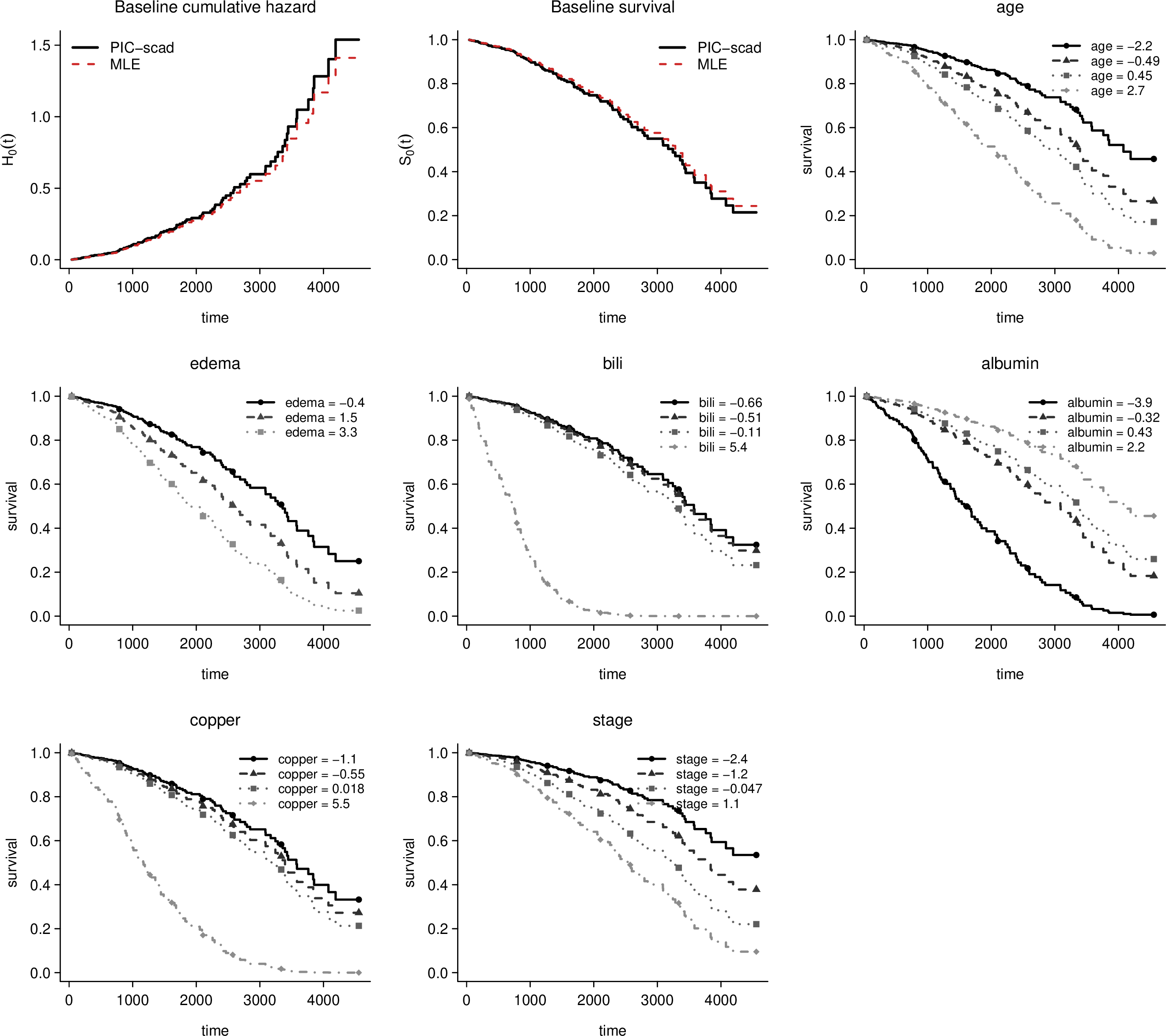
Figure 3: PIC-scad fit on the PBC dataset. The first two panels show the Breslow baseline cumulative hazard \(H_0(t)\) and baseline survival \(S_0(t)\) for the PIC-scad model (solid black) and the full MLE (dashed red). The remaining panels display the effect of each selected covariate on the survival curve, obtained by varying the covariate over representative values while holding all others at their sample mean..
4 Conclusions↩︎
We have introduced PIC-Cox, an extension of the pivotal information criterion to the Cox proportional-hazards model. The method applies a square-root transformation to the partial likelihood, which removes the dependence of the null score on the censoring level \(p_0\), so that the resulting detection boundary \(\lambda_\alpha^{\rm PDB}\) is asymptotically pivotal: its law depends only on the design through \(\Sigma_X = X^{ \mathrm{\scriptscriptstyle T} }X/n\), and on neither the baseline hazard nor the censoring mechanism. This pivotality is what allows the penalty level to be calibrated once, under the null, without cross-validation and without knowledge of any nuisance parameter.
The simulation study and the real-data analyses point to a consistent picture. PIC-Cox performs genuine variable selection with near-exact control of false discoveries, and its two variants trace a favourable complexity–accuracy trade-off: across both
low- and high-dimensional datasets, they attain a predictive C-index comparable or superior to that of the cross-validated lasso, BIC forward selection and the Benjamini–Hochberg-adjusted Cox model, while selecting substantially fewer variables. The
nonconvex PIC-scad variant consistently improves on its convex PIC-lasso counterpart, mitigating the shrinkage bias of the \(\ell_1\) penalty and extending the region of exact support recovery. In
short, PIC-Cox offers what a practitioner most often needs: a compact, well-calibrated model that pinpoints the few covariates driving survival, with neither a tuning parameter to choose nor a nuisance distribution to estimate.
The methodology is implemented in the R package picreg, which fits models following the PIC paradigm across a range of generalized linear models, including linear regression, binary classification, and Cox proportional-hazards regression.
The package is available on CRAN [25] (https://cran.r-project.org/package=picreg), with
documentation at https://vcmaxouuu.github.io/picreg/.
Acknowledgement↩︎
We thank Professor Eva Cantoni for useful comments. This work was partially supported by the Swiss National Science Foundation grant 200021E_213166.
5 Proof of Theorem 1↩︎
Applying Theorem 4 of [10], Cox’s partial likelihood is differentiable everywhere, in particular at \(\boldsymbol{\beta}=\mathbf{0}\). Hence, the smallest value of \(\lambda\) that yields a local minimum at \(\hat{\boldsymbol{\beta}}=\mathbf{0}\) for the PIC criterion 3 with \(\phi(u)=u^{1/2}\) is the zero-thresholding function \[\lambda_0\left(X, \mathbf{y},\boldsymbol{\delta}\right) = \frac{ \left\| \nabla_{\boldsymbol{\beta}} l_n\left(\boldsymbol{\beta}; X, \mathbf{y}, \boldsymbol{\delta}\right) \big|_{\boldsymbol{\beta}=\mathbf{0}} \right\|_\infty }{ 2\{l_n\left(\mathbf{0}; X, \mathbf{y}, \boldsymbol{\delta}\right)\}^{1/2} }.\] Let \(H_0: \boldsymbol{\beta}=\mathbf{0}\) denote the null hypothesis that no covariates affect the survival time. Under \(H_0\), the observed data \((y_i,\delta_i)_{i=1}^n\) form an i.i.d. sample drawn from a distribution that does not depend on \(X\). Throughout this proof, we assume that \((\mathbf{y},\boldsymbol{\delta})\) is generated from this null distribution, with the design matrix \(X\) held fixed, and we study the resulting random variable \(\Lambda=\lambda_0\left(X,\mathbf{y},\boldsymbol{\delta}\right)\).
Following [26], we introduce some counting process notation. Write the counting and at-risk processes \(N_i(t)=I\{y_i\le t,\delta_i=1\}\), \(Y_i(t)=I\{y_i\ge t\}\), and the martingales \(M_i(t)=N_i(t)-\int_0^t Y_i(u)h_0(u)\,\mathrm du\), \(M(t)=\sum_i M_i(t)\). Set the risk-set average \(\bar{\mathbf{x}}(u)=\sum_j Y_j(u)\mathbf{x}_j/\sum_j Y_j(u)\), the at-risk fraction \(\bar Y(u)=n^{-1}\sum_j Y_j(u)\), and \(p_0={\mathbb{P}}(\delta_i=1)\) the probability of being uncensored under \(H_0\).
The statistic can be written as \[\lambda_0\left(X, \mathbf{y},\boldsymbol{\delta}\right) = \frac{\|A_n\|_\infty}{B_n}=\frac{\|\frac{1}{n}\sum_{i=1}^n\delta_i\left(\mathbf{x}_i-\bar{\mathbf{x}}(y_i)\right)\|_\infty}{2\bigl\{\frac{1}{n}\sum_{i=1}^n \delta_i\log{\left(\sum_{j=1}^nY_j(y_i)\right)}\bigr\}^{1/2}}\]
Lemma 1. Under assumptions 1–3, with \(Z\sim\mathcal{N}(0,p_0\Sigma_X)\) and \(\Sigma_X=X^{ \mathrm{\scriptscriptstyle T} }X/n\), \[\sup_{t\in\mathbb{R}}\Bigl|\, {\mathbb{P}}\bigl(n^{1/2}\|A_n\|_\infty\le t\bigr) -{\mathbb{P}}\bigl(\|Z\|_\infty\le t\bigr)\Bigr|\longrightarrow 0 .\]
Proof. Using the counting process, \(A_n=\frac{1}{n}\sum_{i=1}^n\int_0^\tau\left(\mathbf{x}_i-\bar{\mathbf{x}}(u)\right)\,\mathrm{d}N_i(u)\) and substituting the Doob–Meyer decomposition \(\mathrm dN_i=Y_ih_0\,\mathrm du+\mathrm dM_i\), the compensator term \(\int_0^\tau \left(\mathbf{x}_i-\bar{\mathbf{x}}(u)\right)Y_i(u)h_0(u)\mathrm{d}u\) vanishes upon summation over \(i\) by definition of \(\bar{\mathbf{x}}\). Hence, \[n^{1/2}A_n=n^{-1/2}\sum_{i=1}^n \int_0^\tau\mathbf{x}_i\,\mathrm{d}M_i(u)-n^{-1/2}\int_0^\tau\bar{\mathbf{x}}(u)\,\mathrm{d}M(u)=n^{-1/2}\sum_{i=1}^n \mathbf{x}_iM_i(\tau)-n^{-1/2}\int_0^\tau\bar{\mathbf{x}}(u)\,\mathrm{d}M(u).\] Let \(R_n=n^{-1/2}\int_0^\tau\bar{\mathbf{x}}(u)\,\mathrm dM(u)\). Under \(H_0\) and 2 the covariates are centred, \(\sum_{j}\mathbf{x}_j=\mathbf{0}\), and \(Y_j(u)\perp\mathbf{x}_j\), hence the population risk-set average vanishes and \(\bar{\mathbf{x}}(u)\) is exactly the centred empirical process. By the maximal inequality for empirical processes and a union bound over the \(p\) coordinates, \[\sup_{u\in[0,\tau]}\;\|\bar{\mathbf{x}}(u)\|_\infty =O_{{\mathbb{P}}}\!\bigl\{(\log p/n)^{1/2}\bigr\},\] the analogue at \(\boldsymbol{\beta}=\mathbf{0}\) of Lemma E.1 of [27]. For \(k\in\{1,\dots,p\}\), the process \(t\mapsto n^{-1/2}\int_0^t\bar x_k(u)\,\mathrm dM(u)\) is a square-integrable martingale, and by the predictable-variation isometry, with \(\mathrm d\langle M\rangle_u=\sum_{i=1}^n Y_i(u)h_0(u)\,\mathrm du\), \[\mathbb{E}(R_{n,k}^2\mid X) =\mathbb{E}\!\Bigl(\int_0^\tau\bar x_k(u)^2\,\bar Y(u)\,h_0(u)\,\mathrm du\Bigr) \le\Bigl(\sup_{u\in[0,\tau]}\bar x_k(u)^2\Bigr)H_0(\tau) =O_{{\mathbb{P}}}\!\Bigl(\tfrac{\log p}{n}\Bigr),\] uniformly in \(k\), where \(H_0(\tau)=\int_0^\tau h_0<\infty\) by 1 and the last bound uses the previous display. The jumps of \(n^{-1/2}\bar x_k\,\mathrm dM\) are bounded by \(\tilde{B}_n/n^{1/2}\) with \(\tilde{B}_n=B_n\{1+H_0(\tau)\}\), so Bernstein’s inequality for counting-process martingales [28], union-bounded over the \(p\) coordinates, yields \[\|R_n\|_\infty=O_{{\mathbb{P}}}\!\Bigl(\tfrac{\log p}{n^{1/2}}\Bigr) =o_{{\mathbb{P}}}\!\bigl((\log p)^{-1/2}\bigr),\] the last step by assumption 3 since \((\log p)^{3/2}/n^{1/2}\to0\).
Let \(S_n=n^{-1/2}\sum_{i=1}^n\mathbf{x}_iM_i(\tau)=n^{-1/2}\sum_{i=1}^n\mathbf{v}_i\), \(M_i(\tau)=\delta_i-\int_0^\tau Y_i h_0\). Under \(H_0\), \(M_i(\tau)\) depends only on \((T_i,C_i)\) which are i.i.d., hence the \(\mathbf{v}_i=\mathbf{x}_i M_i(\tau)\) are independent. Moreover, \(\mathbb{E}\{M_i(\tau)\}=0\) and, under assumption 1, \[\begin{gather} \mathbb{E}\{M_i(\tau)^2\}=\mathbb{E}\left(\int_0^\tau Y_i(u)h_0(u)\,du\right)= \int_0^\tau {\mathbb{P}}(T\ge u,\;C\ge u)h_0(u)\,du\\ =\int_0^\tau S_T(u)S_C(u)h_0(u)\,du =\int_0^\tau f_T(u)S_C(u)\,du={\mathbb{P}}(T\le C,\;T\le \tau)={\mathbb{P}}(T\leq C)=p_0, \end{gather}\] hence \(\frac{1}{n}\sum_{i=1}^n \operatorname{Cov}(\mathbf{v}_i)=p_0\Sigma_X\) with \(\Sigma_X:=X^{ \mathrm{\scriptscriptstyle T} }X/n\). Under assumption 1, \[|M_i(\tau)|\le|\delta_i|+\int_0^\tau Y_i(u)h_0(u)\,du\le 1+H_0(\tau)<\infty,\] and in particular \(\mathbb{E}\{M_i(\tau)^4\}<\infty\). Under assumption 3, apply the high-dimensional Gaussian approximation of [29] to the independent, centred, bounded vectors \(\tilde{\mathbf{v}}_i=(\mathbf{v}_i,-\mathbf{v}_i)\in\mathbb{R}^{2p}\), with \(Z\sim\mathcal{N}(0,p_0\Sigma_X)\), \[\rho_n:=\sup_{t\in\mathbb{R}}\bigl|{\mathbb{P}}(\|S_n\|_\infty\le t)-{\mathbb{P}}(\|Z\|_\infty\le t)\bigr|\longrightarrow0.\]
It remains to combine the two terms. The Gaussian maximum \(\|Z\|_\infty\) is anti-concentrated: by [30] there is a constant \(C<\infty\) such that \[\sup_{t\in\mathbb{R}}{\mathbb{P}}\bigl(\,|\,\|Z\|_\infty-t\,|\le\varepsilon\,\bigr)\le C\,\varepsilon(\log p)^{1/2} \qquad(\varepsilon>0).\] By our result on \(\|R_n\|_\infty\), pick \(\zeta_n\to0\) with \({\mathbb{P}}(\|R_n\|_\infty>\zeta_n)\to0\) and \(\zeta_n(\log p)^{1/2}\to0\). On the event \(\{\|R_n\|_\infty\le\zeta_n\}\) the inclusion \(\{n^{1/2}\|A_n\|_\infty\le t\}=\{\|-S_n+R_n\|_\infty\le t\}\subseteq\{\|S_n\|_\infty\le t+\zeta_n\}\) holds, hence \[\begin{align} {\mathbb{P}}\bigl(n^{1/2}\|A_n\|_\infty\le t\bigr) &\le{\mathbb{P}}(\|S_n\|_\infty\le t+\zeta_n)+{\mathbb{P}}(\|R_n\|_\infty>\zeta_n)\\ &\le{\mathbb{P}}(\|Z\|_\infty\le t+\zeta_n)+\rho_n+o(1)\\ &\le{\mathbb{P}}(\|Z\|_\infty\le t)+\rho_n+C\zeta_n(\log p)^{1/2}+o(1), \end{align}\] using the Gaussian approximation of \(\|S_n\|_\infty\) then the anti-concentration bound. The reverse inclusion \(\{\|S_n\|_\infty\le t-\zeta_n\}\subseteq\{n^{1/2}\|A_n\|_\infty\le t\}\cup\{\|R_n\|_\infty>\zeta_n\}\) gives the matching lower bound. Taking the supremum over \(t\in\mathbb{R}\), \[\sup_{t\in\mathbb{R}}\bigl|{\mathbb{P}}(n^{1/2}\|A_n\|_\infty\le t)-{\mathbb{P}}(\|Z\|_\infty\le t)\bigr| \le\rho_n+C\zeta_n(\log p)^{1/2}+o(1)\longrightarrow0,\] which is the claim. ◻
Lemma 2. Under assumption 1, \(B_n^2=4\left(p_0\log n+O_{{\mathbb{P}}}(1)\right)\).
Proof. One has \[\frac{1}{n}\sum_{i=1}^n \delta_i\log{\left(\sum_{j=1}^n I\{y_j \ge y_i\}\right)}= \log n\cdot \frac{\sum_{i=1}^n \delta_i}{n} + \frac{1}{n}\sum_{i=1}^n \delta_i\log{\left(\frac{1}{n}\sum_{j=1}^n I\{y_j \ge y_i\}\right)}.\] Since \(\delta_i\) is a binary random variable, \(n^{-1}\sum_{i=1}^n \delta_i=p_0+O_{{\mathbb{P}}}(n^{-1/2})\). So the first term is of order \(p_0\log n + o_{\mathbb{P}}(1)\) as \(n\to\infty\). Moreover, assuming there are no ties, \(\sum_{j=1}^n I\{y_j \ge y_i\}=n-i+1\) and, \[\frac{1}{n}\sum_{i=1}^n \delta_i\log{\left(n^{-1}\sum_{j=1}^n I\{y_j \ge y_i\}\right)} = \frac{1}{n}\sum_{i=1}^n \delta_i\log{\left(\frac{n-i+1}{n}\right)}=:s_n.\] But, \[|s_n|\leq\frac{1}{n}\left|\sum_{i=1}^n\log{\left(\frac{n-i+1}{n}\right)}\right|=-\frac{1}{n}\sum_{i=1}^n\left[\log{(n-i+1)}-\log{n}\right]=\log n - n^{-1}\log n!=O(1),\] using Stirling’s approximation, which gives the result. ◻
Combining Lemmas 1 and 2 via Slutsky’s lemma yields \[2(n\log n)^{1/2}\Lambda = \frac{n^{1/2}A_n}{p_0^{1/2}}\cdot\frac{2(p_0\log n)^{1/2}}{B_n}\xrightarrow{d}\|\mathcal{N}(0, \Sigma_X)\|_\infty.\] The nuisance parameter \(p_0\) cancels, so the limiting law is pivotal in the censoring distribution and depends on the design only through \(\Sigma_X\), which concludes the proof of Theorem 1.
6 Fast Monte Carlo evaluation of \(\lambda_\alpha^{\rm PDB}\)↩︎
By Appendix 5, \(\lambda_\alpha^{\rm PDB}\) is the upper \(\alpha\)-quantile of the random variable \(\Lambda=\lambda_0(X,\mathbf{Y}_0,\boldsymbol{\Delta}_0)\) obtained by evaluating the zero-thresholding statistic ?? on data drawn under \(H_0:\boldsymbol{\beta}=\mathbf{0}\). This appendix shows how to draw each replicate of \(\Lambda\) without ever reordering or copying the design matrix \(X\).
Null draws reduce to a permutation and coin flips↩︎
Under \(H_0\) the pair \((\mathbf{Y}_0,\boldsymbol{\Delta}_0)\) is independent of \(X\), and the observed times are almost surely distinct (continuous failure and censoring laws, no ties). The statistic \(\Lambda\) depends on the data only through (i) the rank ordering of the times, which fixes the nested risk sets and their sizes, and (ii) the event indicators attached to the ordered positions. Since \((\mathbf{Y}_0,\boldsymbol{\Delta}_0)\perp X\), the ranks induce a uniform random permutation \(\pi\) of the covariate rows, independent of the indicators. Moreover, the proof of Theorem 1 shows that the event probability \(p_0={\mathbb{P}}(\delta=1)\) cancels in the ratio \(\Lambda=A_n/B_n\), so its limiting law is invariant to \(p_0\); we may therefore draw the indicators as fair coin flips \(e_i\stackrel{\text{iid}}{\sim}\mathrm{Bernoulli}(1/2)\) rather than \(\mathrm{Bernoulli}(p_0)\). A null replicate of \(\Lambda\) is thus fully specified by a vector \(\mathbf{e}\in\{0,1\}^n\) and a uniform permutation \(\pi\).
Suffix-sum form of the numerator↩︎
Write \(R_i=\{k:y_k\ge y_i\}\) for the risk set at position \(i\) and \(r_i=|R_i|\). With \(\tilde{\mathbf{x}}_i=\mathbf{x}_{\pi(i)}\), the (unnormalized) numerator of ?? under \(H_0\) is \[\mathbf{v}=\sum_{i=1}^n e_i\Bigl(\tilde{\mathbf{x}}_i-\frac{1}{r_i}\sum_{j=1}^i\tilde{\mathbf{x}}_j\Bigr) =\sum_{i=1}^n e_i\tilde{\mathbf{x}}_i -\sum_{i=1}^n\sum_{j=1}^i\frac{e_i}{r_i}\,\tilde{\mathbf{x}}_j .\] Exchanging the order of summation in the double sum, \[\sum_{i=1}^n\sum_{j=1}^i\frac{e_i}{r_i}\,\tilde{\mathbf{x}}_j =\sum_{j=1}^n\tilde{\mathbf{x}}_j\sum_{i\ge j}\frac{e_i}{r_i}.\] Subtracting from \(\sum_i e_i\tilde{\mathbf{x}}_i\) and relabelling the running index \(j\) as \(i\) gives \(\mathbf{v}=\sum_{i=1}^n u_i\,\tilde{\mathbf{x}}_i\) with \[u_i=e_i-\sum_{j\ge i}\frac{e_j}{r_j}.\] Since \(\tilde{\mathbf{x}}_i=\mathbf{x}_{\pi(i)}\), \[\mathbf{v}=\sum_{i=1}^n u_i\,\mathbf{x}_{\pi(i)}=X^{ \mathrm{\scriptscriptstyle T} }\mathbf{u}^{\pi}, \qquad u^{\pi}_{\pi(i)}=u_i,\] that is, \(\mathbf{u}^{\pi}\) is obtained by scattering the entries of \(\mathbf{u}\) through \(\pi\).