Bridging the gap between dark matter and MOND by a relativistc scalar field approach
October 20, 2025
Abstract
A Lagrangian model for a general relativistic scalar field, formulated in the framework of integrable Weyl geometry, is studied. Under the present assumptions it modifies the light cone structure and induces MOND-like dynamics in the weak field approximation of the Einstein frame (gauge). The Lagrangian contains a Bekenstein-type (“aquadratic”) term and a second order term generating additional mass energy for the scalar field. Both are switched on only if the the scalar field gradient is spacelike and below a MOND-typical threshold, like in the superfluid model of Berezhiani/Khoury. In the weak field limit the Bekenstein term implies a deep MOND equation for the scalar field and leads to MONDian free fall trajectories. The Lagrangian mass term induces non-negligible energy and pressures of the scalar field with the respective consequences for gravitational light deflection.
Keywords: scalar field, scale invariance, MOND, radial-acceleration-relation, galaxy, cluster
1 Introduction↩︎
1.1 Basic idea↩︎
This paper shows that under specific conditions for its Lagrangian a gravitationally coupled scalar field can lead to a general relativistic underpinning of modified Newtonian dynamics (MOND) Famaey/McGaugh:MOND?. The model takes up Milgrom’s and Bekenstein’s idea of an “aquadratic” Lagrangian Bekenstein/Milgrom:1984?, Bekenstein:2006?, Bekenstein:2010?, but modifies it in several respects:
(i) It works in the framework of (integrable) Weyl geometry with scale covariant fields, scale invariant expressions for the Lagrangian densities and a gravitationlly coupled scalar field.
(ii) A mass generating term is assumed for the scalar field (in addition to the Bekenstein term). (iii) The Bekenstein and mass terms of the scalar field Lagrangian are assumed to be active only for regions in which the field gradient is spacelike and
below a MOND-typical threshold. The physical reason for this could be a destabilization of the substrate underlying the field dynamics for field gradients above a critical threshold like in Berezhiani/Khoury’s superfluid approach Berezhiani/Khoury:2015?, Berezhiani/Khoury:2016?.
Points (i) and (ii) change the character of the scalar field in comparison with Bekenstein’s. It can no longer be considered exclusively as an enhancement of the gravitational structure like the scalar fields of Jordan-Brans-Dicke (JBD) type. It rather carries also features of some kind of dark matter sui generis, although no particle ontology is assumed. The mass term of the scalar field is its critical pivot; it must not destroy the scalar field equation dominated by the Bekenstein term and ought to have a “reasonable” Hilbert tensor, i.e, one that is essentially divergence free (on shell of the Einstein equation) and is strong enough for modifying the gravitational field such that test particles and light ray structure conform essentially to the expectations of MOND. For the sake of a coherently scale covariant approach the methods and symbolism of Weyl geometric field theory are used.
1.2 Other relativistic generalizations of MOND↩︎
Diverse attempts at general relativistic enhancements of Milgrom’s modified Newtonian dynamics have been made during the last forty years. The first step in this direction has already been made in the appendix of the early paper by Bekenstein and Milgrom Bekenstein/Milgrom:1984?. It is based on a JBD-like scalar field with an “aquadratic” kinetic term and two conformally related Riemannian metrics. This implied, however, a much too small gravitational light deflection. Often the reason is seen in the fact that conformal transformations do not change the light cone structure; the extremely small energy tensor of the Bekenstein scalar field is mentioned only in side remarks. Follow up papers did not try to enhance the mass-energy of the scalar field, but chose the path of drastically modifying the metric, for example by a pair of two “disformal” metrics \(g_{\mu\nu}\) and \(\tilde{g}_{\mu\nu}\), related to each other by a dynamical structure involving a timelike vector field \(A^{\mu}\) in addition to a scalar field \(\phi\). This approach became known under the acronym TeVeS Sanders:1997?, Bekenstein:2004?, Bekenstein:2006?, Bekenstein:2010?.
For nearly two decades TeVeS was the main candidate for a relativistic generalization of MOND. Its two metric hypothesis implied, however, a subluminal propagation speed for tensorial modes of gravitational waves. This led to its empirical devalidation (“refutation”) by the observation of a wave event (GW170817) in August 2017; a comparison with gamma ray signals clearly indicated that gravitational waves propagate on the light cone structure of spacetime.
In the following years two research programs, both in different ways modifying TeVeS, gained attention, the BIMOND (“bimetric MOND”) program of Milgrom, initiated in 2009 (i.e., before GW170817) Milgrom:2009?, Milgrom:2010bimetric?, Milgrom:2022? and the RMOND approach (” new relativistic MOND”) by Skordis and Złośnik published in 2019 Skordis/Zlosnik:2019?, Skordis/Zlosnik:2021?. They still play the central role in the present discourse in the MOND community on relativistic generalizations of their framework. Other attempts at deriving MOND in a general relativistic framework have been made by Berezhiani/Khoury using a superfluid hypothesis Berezhiani/Khoury:2015?, Berezhiani/Khoury:2016?, or Hossenfelder et al. starting from Linde’s “emergent gravity” approach Hossenfelder:2017?, Hossenfelder/Mistele:2018?. Attempts at generalizing MOND in a Weyl geometric framework, different from the one in the present paper, have been proposed by Maeder Maeder:2017?, Maeder:2023? and Harko et al. Burikham/Harko-ea:2023?.
1.3 Organisation of the paper↩︎
In section 2 the fundamentals of the present model are being laid, with its peculiar Lagrangian for a gravitationally coupled scalar field \(\phi\) and with the resulting dynamical equations. The metric satisfies an Einstein equation with an energy tensor of the scalar field in addition to the baryonic source term. The scalar field satisfies a relativistic generalization of the non-linear Poisson equation known from MOND; here it is called the Milgrom equation (section 2.2). The Lagrangian foresees a screening of the scalar field dynamics above a threshold for the field’s gradient, which leaves it effective in weak field constellations only. The dominant terms under such conditions are studied in subsection 2.3. In the flat space limit the Newton approximation of relativistic gravity acquires a potential term \(\Phi^{(\phi)}\) due to the scalar field in addition to the baryonic potential \(\Phi^{(bar)}\). The scalar field satisfies a non-linear Poisson (deep MOND) equation (section 3.1). Both together are called Newton-Milgrom approximation. The flat space potential \(\Phi^{(\phi)}\) allows to draw approximate inferences on the relativistic scalar field \(\phi\) (section 3.2). On the other hand, calculations in the MOND-algorithm with a specific type of MONDian “interpolation” functions become possible in the flat space approximation. They are derived in subsection 3.3.
The next two sections treat special cases. Section 4 focusses on centrally symmetric constellations in baryonic vacuum, which are important for the gravitational environment of stars and of simplified (roundish) model investigations of galaxies. In the inner region the dynamics of the scalar field is suppressed, the Lagrangian reduces to Einstein gravity and leads back to the Schwarzschild solution (section 4.2). In the outer region, with an effective scalar field, the solution of the Milgrom equation contributes an energy tensor to the right hand side of the Einstein equation and shifts the metric away from the Schwarzschild case. This effect is discussed quantitatively in subsection 4.1.
Section 5 deals with galactic dynamics. At first it addresses the radial accelerations of galaxies derived in our model. They are compared with the radial acceleration function empirically determined by McGaugh et al. McGaugh-et-al:2016? in the outskirts of rotationally supported galaxies (section 5.1). A look at recent data of radial velocities in the Milky Way follows; they have given rise to serious doubts as to the feasibility of MOND in general Ou-et-al:2023?, Chan-et-al:2023?. It may therefore come as a surprise that the total accelerations of our model derived from the baryonic density used in Ou-et-al:2023? fit the data quite well, certainly better than MOND with the standard interpolation functions and even better than with the empirical function of McGaugh et al. (section 5.2). Finally a glance is shed at the Newtonian mass equivalent of the scalar field energy in the environment of approximately round galaxies (section 5.3, 6.4).
Open problems are discussed in section 6. The scalar field energy tensor of the scalar field has strong relativistic pressure terms with considerable impact on the light deflection. This may be a critical feature for empirical tests of the approach (section 6.1). Moreover, the scalar field halos of galaxies add mass to the total dynamical mass of clusters. Under plausible assumptions this may become a clue for the dark matter problem in galaxy clusters (section 6.2). On the level of large scale cosmology, on the other hand, the present approach does not change the outlook of Einstein gravity; this may be seen as a plus or as a weak spot (section 6.3). A short look at criticism of MOND in general and the claim of an inconsistency of MOND with recent data on radial velocities in the Milky Way is discussed and rebutted in subsection 6.4.
The paper is rounded off by a resumée (section 7) and an appendix containing some technical explanations (8)
2 Fundamentals↩︎
2.1 Lagrangian↩︎
We start from a scale and diffeomorphism invariant Lagrangian in dimension \(n=4\) \[\mathcal{L} = \mathcal{L}_H(g,\varphi,\phi) + \mathcal{L}_{\phi}(g,\varphi,\phi) + [\mathcal{L}_{bar}(g_E,Y)] \, \label{eq32Lagrangian32general32form}\tag{1}\] with dynamical fields \(g, \phi\), \(Y\) and densities \[\mathcal{L}_X = L_X \sqrt{|g|} \qquad (scale weights w(L_X)=-4)\] for all contributions of type \(X\). Here \(g\) stands for the Riemannian component of a Weylian metric \([(g,\varphi)]\) with scale connection \(\varphi\) which is assumed to be integrable, i.e., non-dynamical (see appendix 8.1). \(\phi\) is a scale covariant scalar field of weight \(w(\phi)= -1\), \(\mathcal{L}_H\) is the gravitational Hilbert term with non-minimally coupled scalar field \[\mathcal{L}_H = \frac{(\hbar c)^{-1}}{2} (\xi \phi)^2 R(g,\varphi) \, \sqrt{|g|} \, . \label{eq32Hilbert32Lagrangian} \qquad\tag{2}\] \(R(g,\varphi)\) is the Weyl-geometric scalar curvature (of weight \(-2\)).2
The Lagrange term of the scalar field \(\mathcal{L}_{\phi}\) appears in two phases or “regimes”, called the Einstein regime, respectively Milgrom regime, depending on the norm of the scalar field gradient (as given by the dynamical equation of the Milgrom regime), \[\mathcal{L}_{\phi} =\epsilon_{\phi} h \, \big( \mathcal{L}_{\phi_2} + \mathcal{L}_{\phi_3}+ \mathcal{L}_{_2\phi} \big) + \mathcal{L}_{V}\, . \label{eq32L-phi32with32h}\tag{3}\] The factor \(h\) is a symbolic expression for the role of a transition function \(h(x, \alpha,\beta)\) which changes smoothly and monotonously between \(0\) in the Einstein regime and \(1\) in the Milgrom regime, see below 10 . One has to keep in mind that we have only sparse empirical information and nearly no theoretical knowledge about the transition between the Einstein/Newton and Milgrom/MOND regimes (but see section 5.2). For the time being, any Lagrangian for it will be unreliable and at best metaphoric. Therefore the dynamics in the transition zone between the two regimes is not derived from the Lagrangian 3 . The intermediate dynamics is rather modelled by a smooth transition, expressed by \(h\), between field solutions formally calculated in the two adjacent regimes.
The factor \(\epsilon_{\phi}\) suppresses the subsequent Lagrange terms for \(\phi\) whenever the gradient of scalar field becomes timelike. Introducing the sign \(s_{\phi}\) of the scalar field gradient we define by\[s_{\phi} = \mathrm{sig}\,D\phi := \mathrm{sig}\,(D_\lambda \phi D^\lambda \phi)\, , \qquad \epsilon_{\phi}= \frac{1}{2}(1+ s_{\phi})\, . \label{eq32convention32epsilon-phi}\tag{4}\] In the Einstein regime and on cosmological scales the scalar field Lagrangian reduces to a quartic potential \[\mathcal{L}_{\phi} =\mathcal{L}_{V}\, .\]
In 1 \(Y\) stands for matter fields based on standard model physics (baryonic matter, elementary particles, electromagnetism). Baryonic matter is assumed to couple to the Riemannian component \(g_E\) of the Einstein gauged Weylian metric. Formally the matter Lagrangian may be written in scale invariant form; this is expressed above by putting \(\mathcal{L}_{bar}(g_E,Y)\) in square brackets.
\(\mathcal{L}_{\phi_2}\) is an ordinary quadratic kinetic term, \(\mathcal{L}_{\phi_3}\) a cubic kinetic term similar to Bekenstein’s “aquadratic” Lagrangian for MOND,3 \(\mathcal{L}_{_2\phi}\) is an additional second order derivative term which endows the scalar field with non-negligible mass-energy without raising the order of the scalar field equation. \(\mathcal{L}_V\) denotes the well known quartic potential term of \(\phi\). A timelike unit vector field (with regard to \(g\)) \(A^{\mu}\) of weight \(w(A)=-1\) has to be assumed as an additional non-dynamical structure for the mass term.4
In scale invariant form the contributions to \(\mathcal{L}_{\phi}\) are \[\begin{eqnarray} \mathcal{L}_{\phi_2} &=&- (\hbar c)^{-1}\frac{\alpha}{2}\,D_{\lambda}(\xi\phi)D^{\lambda}(\xi \phi) \sqrt{|g|} = - (\hbar c)^{-1}\frac{\alpha}{2}\xi^2\,s_{\phi} |D\phi|^2\, \sqrt{|g|} \tag{5} \\ \mathcal{L}_{\phi_3} &=& - \frac{\beta}{3} \phi^{-2} (s_{\phi} D_{\lambda}(\xi \phi)D^{\lambda}(\xi \phi) )^{\frac{3}{2}}\,\sqrt{|g|} = - \frac{\beta}{3} \xi^3 \phi^{-2}|D\phi |^3\,\sqrt{|g|} \tag{6} \\ \mathcal{L}_{_2\phi} &=& (\hbar c)^{-1}\, (\xi \phi)\,D_{\lambda}D^{\lambda}(\xi \phi) A_{\lambda}A^{\lambda}\, \sqrt{|g|} \tag{7} \\ \mathcal{L}_{V} &=& - (\hbar c)^{-3} V(\phi) \,\sqrt{|g|} \, , \qquad here \quad V(\phi)=\lambda\, \phi^4 \, . \end{eqnarray}\] \(\xi\) is a hierarchy factor mediating between the energy levels of the Hilbert term (Planck energy \(E_P\)) and the cosmologically small energy \(E_M=a_0\hbar\) (see below). Later we will find reasons to set \(\alpha = -4,\, \beta= 2\) in the relativistic MOND/Milgrom regime, while effectively \(\alpha=\beta = 0\) in the Einstein/Newton regime.
Let us call the (constant) value of \(\phi\) in the Einstein gauge \(\phi_0\). If we write the scalar field in the Riemann gauge in exponential form, \[\phi(x) \underset{Eg}{\doteq} \phi_0 \, e^{-\sigma(x)} \, , \label{eq32definition32sigma}\tag{8}\] the scale connection in the Einstein gauged Weylian metric becomes \[\varphi \underset{Eg}{\doteq} d\sigma \, .\] Here (and elsewhere) \(\underset{Eg}{\doteq}\) is used to denote equality in the Einstein gauge (see appendix 8.1).
The Lagrangians in Einstein gauge (with identities in this gauge denoted by \(\underset{Eg}{\doteq}\)) turn into: \[\begin{eqnarray}\mathcal{L}_H &\underset{Eg}{\doteq}& \frac{(\hbar c)^{-1}}{2} (\xi \phi_0)^2 R(g,d\sigma) \, \sqrt{|g|} = \frac{(8 \pi \varkappa)^{-1}}{2}\, R(g,d\sigma) \, \sqrt{|g|} \qquad (g=g_E) \\ \mathcal{L}_{\phi_2} &\underset{Eg}{\doteq}& -(\hbar c)^{-1} \frac{\alpha}{2} (\xi \phi_0)^2 \partial_{\lambda} \sigma\, \partial^{\lambda}\sigma\,\sqrt{|g|} = - (8 \pi \varkappa)^{-1}\, \frac{\alpha}{2} (\xi \phi_0)^2 \partial_{\lambda} \sigma\, \partial^{\lambda}\sigma\,\sqrt{|g|} \label{eq32Lagrangian} \\ \mathcal{L}_{\phi_3} &\underset{Eg}{\doteq}& = - \frac{\beta}{3} (\xi^{-1}\phi_0)^{-1} (\xi \phi_0)^2 |\nabla \sigma |^3\,\sqrt{|g|} = - \frac{\beta}{3} a_1^{-1} (8 \pi \varkappa)^{-1}(s_{\phi}\, \partial_{\lambda} \sigma\,\partial^{\lambda} \sigma )^{\frac{3}{2}}\,\sqrt{|g|} \\ \mathcal{L}_{_2\phi} &\underset{Eg}{\doteq}& - (8 \pi \varkappa)^{-1}\, \big(\nabla_{\lambda}\partial^{\lambda}\sigma + \partial_{\lambda}\sigma \partial^{\lambda}\sigma\big) A_{\lambda}A^{\lambda}\, \sqrt{|g|}\, \\ \mathcal{L}_{V} &\underset{Eg}{\doteq}& - (\hbar c)^{-3} \lambda\,(\xi^{-1}\phi_0)^2 (\xi \phi_0)^2 \,\sqrt{|g|} \underset{Eg}{\doteq} - \lambda a_0^2\,c^{-2} (8 \pi \varkappa)^{-1} \sqrt{|g|} \underset{Eg}{\doteq} -\frac{\Lambda}{8 \pi \varkappa} \sqrt{|g|} \, \quad \\ \mathcal{L}_{m} &\underset{Eg}{\doteq}& \ldots \quad (dependent on context) \end{eqnarray}\tag{9}\] With constants \(\xi, \varkappa\) defined in 11 and the line above it. The Lagrangian functions \(L= \mathfrak{L}/ \sqrt{|g|}\) have the dimension of an energy density, \([L]= E\,L^{-3}\), the Lagrange densities \(\mathfrak{L}\) essentially that of an action, more precisely \([c^{-1}\mathcal{L}]=E\,T\) (appendix 8.4).
The transition between the regimes is modelled by a standard function used in differential topology for establishing (\(C^{\infty}\)-) smooth transitions between two structures: \[\begin{align} g(x) &=& \frac{ f(x)}{f(x)+ f(1-x)}\, , \qquad f(x) = \Big\{ { e^{-\frac{1}{x}} \quad for\quad x>0 \atop \; \; 0 \qquad \; for \quad x \leq 0\, , } \nonumber \\ h(x;{\alpha},{\beta}) &=& 1- g\big(\frac{x-{\alpha}}{{\beta}-{\alpha}}\big)\,,\;\;\;\; \; \label{eq32transition32function} \end{align}\tag{10}\] where \({\alpha},\, {\beta}\) define the boundaries of the transition regime. The variable \(x\) may stand for the ratio of the gradient of the scalar field to the MOND constant, \(x = \frac{|\nabla \sigma|}{a_1}\).5
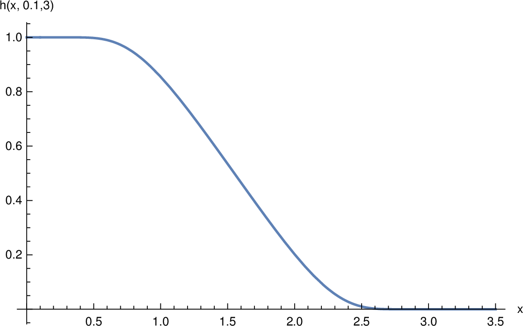
Figure 1: Transition function \(h(x;{\alpha},{\beta})\) for \({\alpha}=0.1,\,{\beta}=3\)..
The suppression of the Lagrange terms 5 , 6 , 7 in the Einstein regime by the factor \(h\) takes up a proposal by Berezhiani and Khoury, developed in their superfluid approach to dark matter and modified gravity in Berezhiani/Khoury:2015?, Berezhiani/Khoury:2016?. Like in this approach we assume that the scalar field can reside in the typical state of the relativistic Milgrom regime only if the norm \(| \nabla \sigma |\) in the Einstein gauge remains below a certain threshold. Once the gradient of \(\sigma\) surpasses the threshold the scalar field destabilizes and a transition phase is entered. Let us call this the lower transition zone.6
For an even larger value of the gradient (as it would be according to the dynamical equations of the Milgrom regime) the dynamics of the actual scalar field \(\bar{\sigma}\) is completely suppressed; \(\nabla \bar{\sigma} \rightarrow 0\). With \(\bar{\sigma}= const\) the scalar field in the Riemann gauge becomes constant, \[\phi \underset{Rg}{\doteq} \phi_0 \, .\] Because of the factor \(\epsilon_{\phi}\) in 3 the same holds for regions in which the model would indicate a shift of the gradient from spacelike to timelike sign.
Finally a suppression of the actual scalar field has to be implemented for a region in which the applicability of the model fades out, called uppper transition zone, by the complementary smooth transition function \[\tilde{h}(x,\hat{\alpha},\hat{\beta})= 1- g(\frac{x-\hat{\alpha}}{\hat{\beta}-\hat{\alpha}}) \, .\]
In the following the usual notation \[\varkappa = G\, c^{-4}\, \qquad (G the Newton gravitational constant)\] is used. Moreover we choose \(\phi_0\) and the hierarchy factor \(\xi\) such that in the Einstein gauge \(\xi\phi_0\) is the Planck energy and \(\xi^{-1}\phi_0\) is the energy associated to the MOND constant \(a_0\): \[(\xi \phi_0) = E_{P}=\big((8 \pi G)^{-1}\, \hbar c^5\big)^{\frac{1}{2}} = \big((8\pi\,\varkappa)^{-1}\, \hbar c \big)^{\frac{1}{2}}\qquad and \quad \xi^{-1}\phi_0 = a_0\, \hbar \, \label{eq32xi32und32phi0}\tag{11}\] This means \[(\xi \phi_0)^{-2} \hbar c = 8 \pi \varkappa.\]
\(a_0\) is a constant of physical dimension \([a_0]=T^{-1}\) with companion \(a_1=a_0\, c^{-1}\) (dimension \([a_1]=L^{-1}\)),7 related to the MOND acceleration \(\mathfrak{a}_0\) by \(\mathfrak{a}_0= a_0\, c\). The empirical value of this acceleration \[\mathfrak{a}_0 \approx 1.8\cdot10^{-8}\, cm\, s^{-2} \, ,\] results in the known approximation \[a_0 \approx \frac{H_0}{6} \quad \longleftrightarrow \quad a_1 = a_0\, c^{-1}\approx \frac{H_1}{6} \qquad \qquad (H_1 = H_0 c^{-1})\,.\] The hierarchy factor \(\xi\) is chosen such that \(\phi_0\) is placed at the geometrical mean between the cosmologically small energy scale \(E_M= a_0\hbar \sim 10^{-32}\, eV\) ( \(\sim \frac{H_0}{6} \hbar\)) which may be called Milgrom energy and the reduced Planck energy \(E_P\sim 10^{27}\, eV\). Its order of magnitude is \(\xi \sim 10^{30}\). Of course, this convention may be changed if preferred.
In the Einstein gauge the quartic potential \(L_V\) degenerates into a cosmological constant term with coefficient \(\frac{\Lambda}{8\pi G}c^{-2}\). The above choice of \(\phi_0\) (in the geometric mean of the extremes) results in a moderate order of magnitude for \(\lambda\). Using the usual notation \(\Omega_{\Lambda}\) one finds: \[\lambda\, a_1^2 = \Lambda = 3 \, \Omega_{\lambda}\, H_1^2 \qquad \longleftrightarrow \quad \lambda \approx 3\cdot 6^2 \, \Omega_{\Lambda}\,\]
2.2 Dynamical equations↩︎
Einstein equation
The variational derivation \(\delta g^{\mu\nu}\) of the Hilbert term 2 leads to the Weyl geometric Einstein tensor \(G_W = G(g, d\varphi)\) plus an
additional term due to the variation of the non-minimally coupled scalar field:8 \[(\xi \phi)^{-2} \big(g_{\mu\nu}\, D_{\lambda}D^{\lambda}(\xi
\phi)^2 - D_{(\mu}D_{\nu)}(\xi\phi)^2 \big) \,\] Brought to the right hand side (r.h.s.) as \[\Theta^{(\phi_H)} = - (\xi \phi)^{-2} \big(g_{\mu\nu}\, D_{\lambda}D^{\lambda}(\xi \phi)^2 - D_{(\mu}D_{\nu)}(\xi\phi)^2
\big)\] it contributes to the effective scalar field energy momentum of the vacuum Einstein equation \[G_W = G(g, d\varphi) = \Theta^{(\phi)} + \Theta^{(\phi_H)} \, .\] \(\Theta^{(\phi)}\) is the energy term arising from the variational derivative of \(\mathcal{L}_{\phi}\) (here denoted by \([ \mathcal{L}_{\phi} ]_{g^{\mu\nu}}\)),
\[\Theta^{(\phi)} = - \frac{2 (\hbar c)}{\sqrt{|g|}} (\xi \phi)^{-2} [ \mathcal{L}_{\phi} ]_{g^{\mu\nu}} \underset{Eg}{\doteq} -\frac{2}{\sqrt{|g|}}\, 8\pi \varkappa \,[\mathcal{L}_{\phi}]_{g^{\mu\nu}}\, .\] Its
corresponding energy tensor is \[T^{(\phi)}_{\mu\nu} = - \frac{2}{\sqrt{|g|}} [\mathcal{L}_{\phi} ]_{g^{\mu\nu}} = (\hbar c)(\xi \phi)^2 \Theta^{(\phi)} \underset{Eg}{\doteq} 8 \pi \varkappa\, \Theta^{(\phi)} \, .\]
If baryonic matter is included a similar energy expression for baryonic matter \(\Theta^{(bar)}\) appears on the r.h.s. of the Einstein equation, corresponding to a matter energy-momentum tensor formally written in scale covariant form, \[T^{(bar)}_{\mu \nu} = - \frac{2}{\sqrt{|g|}} [\mathcal{L}_{bar} ]_{g^{\mu\nu}} = (\hbar c)(\xi \phi)^2 \Theta^{(bar)} \, .\]
Because of the coupling condition for matter the Einstein equation with baryonic matter is best expressed in the Einstein gauge \[G_W \underset{Eg}{\doteq} G(g_E, d\sigma) \underset{Eg}{\doteq} (8\pi\varkappa)\, T^{(bar)}_E + \Theta^{(\phi)}_E + \Theta^{(\phi_H)}_E \, . \label{eq32Einstein32eq32with32matter}\tag{12}\] The subscript \(E\) indicates that all terms on the r.h.s. are understood in their Einstein gauge. In the following this will be presupposed even without the subscript for the r.h.s of a \(\underset{Eg}{\doteq}\) relation. For bringing the form of 12 closer to Einstein gravity we decompose the l.h.s. into its Riemannian component and the scale connection contribution (see appendix 8.1) \[G_W \underset{Eg}{\doteq} G(g) + G(d\sigma) \, ,\] with \(G(d\sigma)\) give by 78 . Shifting it to the r.h.s becomes \[G(g) \underset{Eg}{\doteq} (8\pi\varkappa)\, T^{(bar)} + \Theta^{(\phi)} + \Theta^{(\phi_H)} - G(d\sigma) \, . \label{Weylgeometric32EEq320}\tag{13}\]
In dimension \(n=4\) the second order derivative terms of \(\Theta^{(\phi_H)}\) and \(G(d\sigma)\) cancel, the added contributions of the scalar field in 13 simplify to: \[\bar{\Theta}^{(\phi)}_{\mu\nu} \underset{Eg}{\doteq} \Theta^{(\phi)}_{\mu\nu} - 3 \partial_{\lambda}\sigma \partial^{\lambda}\sigma\, g_{\mu \nu} + 6 \partial_{\mu}\sigma \partial_{\nu}\sigma \,. \label{eq32full32scalar32field32energy32expression}\tag{14}\] \(\bar{\Theta}^{(\phi)}\) sums up all contributions of the scalar field to the r.h.s. of the Einstein equation, including its gravitational contributions (deriving from the Hilbert term and the scale connection part of the Einstein tensor) on a par with its energy expression proper \(\Theta^{(\phi)}\). The final form of the gravitational equation for \(n=4\) in the Einstein gauge is then \[G(g) \underset{Eg}{\doteq} (8\pi\varkappa)\, T^{(bar)}_E + \bar{\Theta}^{(\phi)}\, . \label{Weylgeometric32EEq}\tag{15}\] Note, however, that neither \(\bar{\Theta}^{(\phi)}\) nor its energy tensor \[\bar{T}^{(\phi)}_{\mu\nu} \underset{Eg}{\doteq} (8 \pi \varkappa)^{-1} \bar{\Theta}^{(\phi)}_{\mu \nu} \,\] is scale covariant because of the contributions from \(G(\varphi)\). It will thus be used in the Einstein gauge only.
After evaluating all contributions to \(\Theta^{(\phi)}\) in the Milgrom regime this is \[\begin{align}
\bar{\Theta}^{(\phi)}_{\mu \nu} &\underset{Eg}{\doteq}&
\Box(g)\sigma(g_{\mu\nu} + 2 A_{\mu}A_{\nu}) - 2 \nabla(g)_{(\mu}\partial_{\nu)} \sigma \label{eq32Theta-phi-bar} \\ & & + (\alpha+12)\,\partial_{\mu}\sigma\partial_{\nu}\sigma + 2 \,\partial_{\lambda}\sigma\partial^{\lambda}\sigma A_{\mu}A_{\nu} -
\big((\frac{\alpha}{2} +3)\partial_{\lambda}\sigma\partial^{\lambda}\sigma + \frac{2 \beta}{3} a_1^{-1}\, | \nabla \sigma |^3 + \Lambda \big)g_{\mu\nu}\, . \nonumber
\end{align}\tag{16}\] Outside the Milgrom regime it reduces to \(\bar{\Theta}^{(\phi)}_{\mu \nu} \underset{Eg}{\doteq} \Lambda g_{\mu\nu}\), i.e., the cosmological term of Einstein gravity.
Scalar field equation
Baryonic matter does not couple directly to the scalar field. In the Milgrom regime the scalar field equation \[[\mathcal{L}]_{\phi} = [{L}]_{\phi} = \sum_{X\in {\phi_2,\phi_3,_2\phi,V}} [{L}_X]_{\phi} = 0\] gives term by
term:9 \[\begin{align} 2 \phi^{-1} {L}_H
&+& \alpha \xi^2 D_{\lambda} D^{\lambda}\phi \label{eq32rough32scalar32field32equation} \\
&+& 4 \phi^{-1} {L}_{\phi_3} + \,s_{\phi}\,\, \beta\, \xi^3 \phi^{-2} D_{\lambda}\big(|D \phi|D^{\lambda}\phi \big)
+ 2 \, \xi^2 D_{\lambda}D^{\lambda} \phi\,A_{\lambda}A^{\lambda}
+ 4 \phi^{-1} {L}_{V} = 0 \nonumber
\end{align}\tag{17}\] On shell of the Einstein equation the scalar field equation is obviously equivalent to \[2\, tr\,[\mathcal{L}]_g + \phi [\mathcal{L}]_{\phi} = 0 \, .\] This condition for \(\phi\) will be called the reduced scalar field equation. Like in JBD theory it encodes an indirect coupling, mediated by the Hilbert term, between baryonic matter and the scalar field.
With 83 , 90 , 17 and setting \[\alpha=-4 \label{eq32alpha}\tag{18}\] the reduced scalar field equation becomes \[\begin{align} s_{\phi} \beta\,\xi^3 \phi^{-1}\, D_{\lambda} (|D\phi| D^{\lambda}\phi) &+& 2 \,(\hbar c)^{-1}\,\xi^2 D_{\lambda}\phi D^{\lambda}\phi + 3 \mathcal{L}_{\phi_3} \nonumber \\ &+& 2\,(\hbar c)^{-1}\,\xi^2 (1 + A_{\lambda}A^{\lambda} )\, \phi\, D_{\lambda}D^{\lambda}\phi = tr\, [T^{(bar)}]\, . \end{align}\] The unit condition for the non-dynamical vector field \(A^{\mu}\) simplifies it to \[s_{\phi} \beta\,\xi^3 \phi^{-1}\, D_{\lambda} (|D\phi| D^{\lambda}\phi) + 2 \,(\hbar c)^{-1}\,\xi^2 D_{\lambda}\phi D^{\lambda}\phi + 3 \mathcal{L}_{\phi_3} = tr\, [T^{(bar)}]\, . \label{eq32reduced32SF32long}\tag{19}\] For spacelike \(\nabla \sigma\) in the Milgrom regime (\(s_{\phi}=1\)) this is10 \[\nabla(g)_{\lambda}(|\nabla \sigma |\partial^{\lambda}\sigma \big) - 2 \beta^{-1}\, a_1 |\nabla \sigma|^2 + |\nabla \sigma|^3 \underset{Eg}{\doteq} - a_1 \, \beta^{-1} (8 \pi \varkappa)\, tr\, T^{(bar)} \, . \label{eq32full32Milgrom32equation}\tag{20}\] Both sides of the equation are of dim \(L^{-3}\).
The last two terms on the l.h.s. together form a cubic polynomial in \(|\nabla \sigma|\), \[p_3(x) = (x - 2 \beta^{-1} a_1)\, x^2 \, .\] In the Milgrom regime with \(|\nabla\sigma| \leq a_1\) and \(\beta = 2\) it is negligible: \[|p_3(|\sigma|)| \leq c^{-3} a_0^3 < c^{-3}H_0^3 \ll \Lambda \,\] Therefore it is justified to represent 20 in the simpler approximate form \[\nabla(g)_{\lambda}(|\nabla \sigma |\partial^{\lambda}\sigma \big) \underset{Eg}{\doteq} - \mathfrak{a}_0 \beta^{-1}\, (8 \pi \varkappa)\, c^{-2}\,tr\, T^{(bar)} \, . \label{eq32core32Milgrom32equation}\tag{21}\] This approximation will be called the relativistic Milgrom equation of the present model. It is a straight forward covariant generalization of the nonlinear Poisson equation of deep MOND.
2.3 The scalar field energy tensor in weak fields↩︎
The first order derivatives appear in quadratic or cubic monomials. In weak field constellations the energy-momentum is therefore dominated by the second order derivative terms of \(\sigma\), because .We thus concentrate
on the second order expressions in 16 denoted by \(\hat{\Theta}^{(\phi)}\) and \(\hat{T}^{(\phi)}\): \[\begin{eqnarray}
\hat{\Theta}^{(\phi)}_{\mu\nu} &\underset{Eg}{\doteq}& \Big( \Box(g)\sigma \, (g_{\mu\nu} + 2\, A_{\mu}A_{\nu}) - 2\, \nabla(g)_{(\mu} \partial_{\nu)}\sigma \Big) \, \tag{22} \\ \hat{T}^{(\phi)}_{\mu\nu} &\underset{Eg}{\doteq}& (8 \pi
\varkappa)^{-1} \hat{\Theta}^{(\phi)}_{\mu\nu} \, \tag{23}
\end{eqnarray}\] Both are traceless.
16 becomes then \[\bar{\Theta}_{\mu\nu} \underset{Eg}= \hat{\Theta}_{\mu\nu} + p_{\mu\nu} + \Lambda g_{\mu\nu}\, ,\] where \(p_{\mu\nu}\) are the
components of a tensor \(p(d\sigma)\) given by third degree polynomials in the partial derivatives.11
Focussing attention on the second order terms the full the energy tensor can be written as \[\bar{T}^{(\phi)} \underset{Eg}= \hat{T}^{(\phi)} + (8\pi \varkappa)^{-1}\big( \Lambda\, g_{\mu\nu} + p(\partial\sigma) \big)\, \label{eq32full32energy32tensor32phi}\tag{24}\] and the Einstein equation as \[G(g) \underset{Eg}= 8\pi \varkappa\, \big(T^{(bar)} + \hat{T}^{(\phi)} \big) + \Lambda g + p(\partial\sigma) \, . \label{eq32Einstein32equation}\tag{25}\] In cases where the polynomial and the cosmological term can be neglected, the full Einstein equation may be substituted by the approximation \[G(g) \underset{Eg} \approx 8\pi \varkappa\, \big(T^{(bar)} + \hat{T}^{(\phi)}\big) \, ; \label{eq32Einstein32equ32simplified}\tag{26}\] remember that \(\hat{T}^{(\phi)}\) contains only second order derivates of \(\sigma\).
For quasi-static spacelike \(\nabla \sigma\), \(A_0=1\) and \(g_{00}\approx -1\) the dominant second order terms of the energy component of 23 reduce to12 \[\rho^{(\phi)} \underset{Eg} = \hat{T}^{(\phi)}_{00} \approx (8 \pi \varkappa)^{-1} \, \Box(g)\sigma = (8 \pi \varkappa)^{-1} \, \nabla^2(g) \sigma \, , \, \label{eq32energy32component32scalar32field}\tag{27}\] with \(\nabla^2(g)\) the Laplacian with regard to \(g\).
Because of \(tr\, \hat{T}^{(\phi)}= 0\) the expression entering the weak field approximation of Einstein gravity is also \[\hat{T}^{(\phi)}_{00} - \frac{1}{2}tr\, \hat{T}^{(\phi)}g_{00} \approx (8 \pi \varkappa)^{-1} \, \nabla^2(g)\sigma \, . \label{eq32rhs32scalar32field32contribution32to32Newton32approximation}\tag{28}\]
3 Flat space approximation: a special type of MOND dynamics↩︎
3.1 Newton approximation and deep MOND equation for the scalar field↩︎
Gravity
Let us consider a Riemannian component of the metric for a quasi-static mass distribution, \[g_{\mu\nu} = \eta_{\mu\nu} + h_{\mu \nu} \qquad(signature (-+++))\, ,
\label{eq32weak32field32metric}\tag{29}\] where \(\eta\) is the Minkowski metric and \(h\) is diagonal with small entries (both in special relativistic dimensional conventions
\([\eta]=[h]=1\)). For the Einstein equation rewritten as \[Ric = 8 \pi \varkappa \big(T- \frac{1}{2}tr\, T\, g \big)\] there is a well known first order approximation of the energy
component of the l.h.s.: \[R_{00} \approx - \frac{1}{2} \eta^{\lambda \lambda}\partial_{\lambda} \partial_{\lambda}h_{00}= - \frac{1}{2} \delta^{jj} \partial_j\partial_j h_{00}
\, . \label{eq32Ri0j032weak32field}\tag{30}\] After defining a potential \[\Phi := -\frac{1}{2}c^2\, h_{00} \label{eq32Phi32--32h00}\tag{31}\] the ensuing
relation \[\nabla^2 \Phi \approx c^2 R_{00} = (8\pi \varkappa) c^{2}(T_{00}-\frac{1}{2}tr T\, g_{00}) = (4\pi G)c^{-2}\, (2\, T_{00}-tr T\, g_{00})\,
\label{eq32Poisson32equation32Newton32approximation320}\tag{32}\] is the Newton approximation of Einstein gravity. For \(T^{(bar)}\) of pressure free matter with energy density \(\rho_e\), i.e., mass density \(\rho_m= c^{-2} \rho_e\), this is the usual Poisson equation \(\nabla^2 \Phi = 4\pi G\, \rho_m\).
In our case with \(T=T^{(bar)} + \hat{T}^{(\phi)}\) we add the scalar field contribution using 28 \[(8\pi
G)c^{-2}\, (\hat{T}^{(\phi)}_{00} - \frac{1}{2} tr \hat{T}^{(\phi)} g_{00} ) \approx \nabla^2(g) \sigma\, .\] According to 27 this is \[\nabla^2(g) \sigma = (4 \pi
G)\,c^{-2}\, 2\, \rho^{(\phi)} = 4\pi G\, 2\, \rho^{(\phi)}_m \, .\] The symbol \(\rho^{(\phi)}_m\) is here used for the mass density corresponding to the scalar field energy density,
\[\rho^{(\phi)}_m = c^{-2} \rho^{(\phi)} \, , \label{eq32mass32density32scalar32field}\tag{33}\] without raising an ontological claim of the
“mass”-ness for the scalar field. It differs from the Newtonian mass equivalent of the scalar field energy, which one would expect from the Poisson equation of pressure free matter (see 37 ).
Evaluation of 32 for pressure free baryonic matter and the scalar field together results in a Poisson equation of the form
\[\nabla^2 \Phi = 4\pi G\, \big(\rho^{(bar)}_m + 2\, \rho^{(\phi)}_m \big)\, \label{eq32Poisson32equation32Newton32approximation}\tag{34}\]
(denoting here the baryonic mass density by \(\rho^{(bar)}_m\) and with “\(=\)” the equality in the flat space approximation).
The total Newton potential is a superposition of contributions from the baryonic matter and the scalar field \[\Phi = \Phi^{(bar)} + \Phi^{(\phi)}\, \qquad with\quad \nabla^2 \Phi^{(bar)} = 4\pi G \, \rho_m\,, \quad \nabla^2 \Phi^{(\phi)} = 4 \pi G\, 2 \rho^{(\phi)}_m\,. \label{eq32total32potential32Newton32approximation}\tag{35}\] Because of the pressure term the relativistic mass-energy density of the scalar field enters the potential of the Newton approximation with (relative) factor 2. If one defines the Newtonian mass equivalent \(\rho^{(\phi)}_N\) of the scalar field as the source of the usual Newtonian Poisson equation, \[\Delta \Phi^{(\phi)} = 4\pi G\, \rho^{(\phi)}_N\, ,\] one finds \[\rho^{(\phi)}_N = c^{-2} 2\, \rho^{(\phi)} \, . \label{eq32Newtonian32mass32equivalent32phi322}\tag{36}\] It differs from the “true” mass density associated to the (field theoretic) energy density of the scalar field 33 by the factor \(2\). In certain contexts it is called the density of “phantom matter”.
A comparison with 27 shows \[\Phi^{(\phi)} = c^2\, \sigma \, .\label{eq32Phi-phi}\tag{37}\] Up to the factor \(c^2\) the scalar field potential of the flat space approximation is given by the exponential \(\sigma\) of the scalar field in Riemann gauge 8 .
The total acceleration \(a\) of test masses in the Newton approximation is \[a = -\nabla \Phi= a^{(bar)} +a^{(\phi)} \qquad with \quad a^{(bar)}= - \nabla \Phi^{(bar)}\,, \quad a^{(\phi)} = -\nabla \Phi^{(\phi)}= - c^2\,\nabla \sigma \, \label{eq32additional32acceleration32phi}\tag{38}\] and the boundaries of the transition interval of 10 may be rewritten as \[\bar{\alpha}\, a_0 \leq |a^{(\phi)}| \leq \bar{\beta}\, a_0 \qquad with, e.g., the choice of\bar{\alpha} = 0.1\,, \; \bar{\beta}= \,3\; (see fn. \ref{fn32alpha32beta}). \label{eq32boundaries32transition32region}\tag{39}\]
Scalar field
For pressure free matter with matter density \(\rho^{(bar)}_{m}\) (dimension \(ML^{-3}\)) the r.h.s. of 21 turns into \(\mathfrak{a}_0 \beta^{-1}\, 8 \pi \varkappa\, \rho^{(bar)}_m\).13 This suggests to set \[\beta = 2 \, . \label{eq32beta}\tag{40}\]
By multiplying with \(c^4\) and replacing \(\sigma\) with the potential \(\Phi^{(\phi)}\), the relativistic Milgrom equation 21 for pressure free quasi-static matter turns into \[\nabla(g)_{\lambda}\,(|\nabla \Phi^{(\phi)} |\partial^{\lambda}\Phi^{(\phi)}\big) = \mathfrak{a}_0 \, (4 \pi G)\, \rho^{(bar)}_m \, . \label{eq32approximate32Milgrom32equation}\tag{41}\]
In the notation of vector calculus in the weak field limit (with \(\nabla(g) \rightarrow \nabla\) of flat space) this is \[\nabla
\cdot\big(|\nabla \Phi^{(\phi)}| \nabla \Phi^{(\phi)}\big) = \mathfrak{a}_0 \, (4 \pi G)\, \rho^{(bar)}_m \, . \label{eq32flat32space32Milgrom32equation}\tag{42}\] In other words, the scalar field potential \(\Phi^{(\phi)}= c^2 \sigma\) 37 satisfies the deep MOND equation of the usual MOND appraoch.14
Intermediate Result:
The total potential in the Newton approximation 35 of our model is a sum of the Newtonian matter potential \(\Phi^{(bar)}\) and a deep MOND potential \(\Phi^{(\phi)}\) due to the scalar field 42 . Together they form the Newton-Milgrom approximation of the scalar field model. Its phenomenology places it in the family
of MOND models while it has peculiar features which give it its own distinctive flavour. They are explored in the sequel.
3.2 Inferences from the flat space approximation on the scalar field halo↩︎
The calculations in the flat space approximation can be used for investigating properties of the relativistic model by a kind of reverse Milgrom approximation. Starting from data and calculations in the flat space approximation one can infer
the approximate value of the scalar field potential:
Assume that for a given classical baryonic mass density \(\rho^{(bar)}\) in the Milgrom regime the Newton potential \(\Phi^{(bar)}\) in flat space is given, and its induced acceleration is
\[a^{(bar)} = -\nabla \Phi^{(bar)} \qquad (dimension LT^{-2}) \, .\] Then the acceleration \[\bar{a} = \sqrt{\frac{\mathfrak{a}_0}{
|a^{(bar)}|}}\, a^{(bar)} = \sqrt{\mathfrak{a}_0 |a^{(bar)}|}\, \frac{a^{(bar)}}{|a^{(bar)}|} \, \label{eq32algebraic32transformation32a}\tag{43}\] is the (negative) gradient of a scalar potential \(\bar{\Phi}\) satisfying 42 like \(\Phi^{(\phi)}\).15
Proof: Using the duality in Euclidean space between vector fields and 1-forms, \(a^{(bar)}\) may be conceived a closed 1-form (on flat space), \(d a^{(bar)}=0\). Thus also \(d \bar{a}=0\); and the integrability of \(\bar{a}\) follows (flat space is simply connected). Choose any of its integrals, \[\bar{\Phi} = - \int \bar{a} \, \qquad \longleftrightarrow \qquad
\nabla \bar{\Phi} = - \,\bar{a} . \label{eq32definition32sigma-bar}\tag{44}\] A straight forward vector calculation shows that \(\bar{\Phi}\) satisfies the equation 42 . \(_\square\)
Because of the non-linearity of equation 42 this does not in general imply equality of \(\bar{\Phi}\) with any other solution of the equation (up to an additive
constant).16 But we consider and define it as the main solution of 42 and continue to work with \[\Phi^{(\phi)} = \bar{\Phi} \, .\] Then \(a_{\phi}=\bar{a}\), and the total acceleration in the Milgrom regime is \[a = a^{(bar)} + \bar{a}= a^{(bar)} \, \big(1 + \sqrt{\frac{\mathfrak{a}_0}{|a^{(bar)}|}} \big)\, . \label{eq32total32acceleration32Milgrom32regime}\tag{45}\]
The fictitious matter density \(\bar{\rho}\) corresponding to \(\bar{\Phi}=\Phi^{(\phi)}\) calculated in flat space according to Newton gravity is \[\bar{\rho}=
- (4 \pi G)^{-1}\,\nabla \cdot \,\bar{a} = (4 \pi G)^{-1}\, \nabla^2 \bar{\Phi} \, ,\] This is an approximation for the Newtonian mass equivalent of the scalar field 36 (respectively the
phantom matter density mentioned above).
Because of 43 \[\nabla \cdot \bar{a} = a^{(bar)}\cdot \nabla\big( \sqrt{\frac{\mathfrak{a}_0}{|a^{(bar)}|}} \big) +
\sqrt{\frac{\mathfrak{a}_0}{|a^{(bar)}|}} \cdot \nabla a^{(bar)} \, ,\] and thus \[\bar{\rho} = (8\pi
G)^{-1}\sqrt{\frac{\mathfrak{a}_0}{|a^{(bar)}|^3}}\, \big(a^{(bar)} \cdot \nabla |a^{(bar)}|\big) + \sqrt{\frac{\mathfrak{a}_0}{|a^{(bar)}|}} \rho^{(bar)} \,. \label{eq32mass-energy32scalar32field32in32flat32case}\tag{46}\] The first term
expresses a flat space approximation of the phantom mass-energy generated in matter free regions of a changing Newtonian acceleration field induced by baryonic matter, the second one adds energy proportional to the baryonic matter density. Because of 34 the density 46 calculated according to the Newtonian Poisson equation (in this sense “phantom”) is twice the energy density of
the scalar field converted to mass and equal to its total Newtonian mass equivalent 36 , \[\bar{\rho} \approx \rho_N^{(\phi)} \approx 2\, c^{-2}\rho^{(\phi)}_e
\,.\]
3.3 MOND “interpolation” functions↩︎
In this subsection \(a_N\) denotes the Euclidean norm of the Newtonian acceleration of baryonic mass, \(a_N = |a^{(bar)}|\); the symbol \(a\) is used here
as an abbreviation for the modulus of the dynamically effective total acceleration (not the whole vector as at other places).
In classical (flat space) MOND the functional relationship between \(a_N\) and \(a\) is expressed by two functions called “interpolation” functions,17 \[a = \tilde{\nu}(a_N)\, , \quad \quad a_N= \tilde{\mu}(a)\,, \quad with mutually inverse functions \quad \tilde{\nu}\circ\tilde{\mu}= id\, .\] This relationship is
independent of the baryonic mass distribution of individual galaxies. The \(\tilde{\nu}\)-relation plays an important role in empirical studies; its specification for disk galaxies is called the radial acceleration
relation (see section 5.1).
For emphasizing the role of the typical constant acceleration \(\mathfrak{a}_0= c\, a_0\) below which \(\tilde{\nu}\) and \(\tilde{\mu}\) deviate from the identity the transformation is usually expressed in the form \[\tilde{\nu}(a_N)= \nu(\frac{a_N}{\mathfrak{a}_0})a_N = a\, , \quad \tilde{\mu}(a)=\mu(\frac{a}{\mathfrak{a}_0})a = a_N \, . \label{eq32mu32nu32MOND32defined}\tag{47}\] In the MOND literature \(\mu\) and \(\nu\) come always in pairs but are not uniquely determined. Because of 47 every pair satisfies the constitutive relationship: \[\mu(x)\, \nu(y)=1 \quad for variables x, \, y such that \quad \mu(x)\, x = y \; and \; \nu(y) \, y = x \, . \label{constitutive32relation32mu32nu}\tag{48}\] Moreover two asymptotic conditions have to be satisfied: \[\begin{align} \mu(x) \overset{x\to \infty}{\longrightarrow} 1\,, &\quad & \nu(y)\overset{y\to \infty}{\longrightarrow} 1 \qquad \quad (upper asymptotic) \label{eq32asymptotic32conditions}\\ \mu(x) \overset{x\to 0}{\longrightarrow} x \; \, , &\quad & \nu(y) \overset{y\to 0}{\longrightarrow} y^{-\frac{1}{2}} \qquad (lower asymptotic) \nonumber \end{align}\tag{49}\] (where \(\mu(x) \overset{x\to 0}{\longrightarrow} x\) is understood in the sense of \(\frac{x}{\mu(x)} \overset{x\to 0}{\longrightarrow} 1\)).
By setting \(x= \frac{a}{\mathfrak{a}_0}\) and \(y=\frac{a_N}{\mathfrak{a}_0}\) any pair of functions satisfying the constitutive relationship and the asymptotic condition defines an algorithmic MOND model for galactic dynamics. The upper condition of 49 then expresses the asymptotic transition to Newton dynamics, the lower one the transition to the so-called deep MOND regime characterized by the limit condition \[a=\sqrt{\mathfrak{a}_0a_N} \, .\] The upper condition should be satisfied not only asymptotically, but convert to Newtonian dynamics already for \(x\) (respectively \(y\)) above a finite value, at least in an extremely good approximation.
A typical family of elementary algebraic functions, indexed by \(n\), is Famaey/McGaugh:MOND?, \[\mu_n(x)= x (1+x^n)^{-\frac{1}{n}} \, , \qquad \nu_n(y) = \Big(\frac{1}{2}\big(1+ (1+ 4 y^{-n} \big)^{\frac{1}{2}} \Big)^{\frac{1}{n}}\,, \quad n= 1, 2, 3 \ldots \label{eq32simple32interpolation32functions}\tag{50}\] For basic considerations often the pair of simple transformation functions \((\mu_1, \, \nu_1)\) suffices. In his first study of the so-called “mass deficiency – acceleration relation” McGaugh:2004? McGaugh prefers the quadratic one \((\mu_2, \nu_2)\) (for a more refined study see section 5.1).
We directly read off the MONDian interpolation function \(\nu\) of our model in the Milgrom regime from 45 : \[\nu(y) = 1 + y^{-\frac{1}{2}}\, \label{eq32nu-M}\tag{51}\] The transition between the Milgrom and the Einstein/Newton regimes takes place for \(y=\frac{a_N}{a_0}\) between \(\bar{\alpha}\) and \(\bar{\beta}\). We model this by the smoothing function 10 \[h(y;\bar{\alpha},\bar{\beta}) \qquadwith, e.g., \bar{\alpha}= 0.1, \; \bar{\beta}= 3 \] and set \[\nu_{\mathtt{sf}}(y) = 1 + h\, y^{-\frac{1}{2}}\] Solving the equation \(\nu(\frac{a_N}{\mathfrak{a}_0}) a_N = a\) for \(a_N\) and solving the relation \(y= \mu(x)\cdot x\) 48 for \(\mu(x)\) leads to \(\mu(x) = \frac{ 1}{2x}(2x + h^2- h \sqrt{h^2 + 4x} )\).18
The complete interpolation functions of the scalar field model, including shading, are19 \[\begin{eqnarray} \nu_{\mathtt{sf}} (y) &=& 1 + h \, y^{-\frac{1}{2}} \, , \qquadwith \; h= h(x;\tilde{\alpha}, \tilde{\beta}) \tag{52} \\ \mu_{\mathtt{sf}} (x) &=& \frac{ 1}{2x}(2x + h^2- h \sqrt{h^2 + 4x} )\, , \qquad h=h(x,\bar{\alpha},\bar{{\beta}})\, , \tag{53} \end{eqnarray}\] and thus \[\begin{eqnarray} a &=& a_N + h \sqrt{a_N \mathfrak{a}_0} \label{eq32a40a-N41-sf} \\ a_N &=& \mu_{\mathtt{sf}}(\frac{a}{\mathfrak{a}_0})\,a = a + \frac{\mathfrak{a}_0}{2}\Big(h^2- h \sqrt{h^2+\frac{4a}{\mathfrak{a}_0}}\,\Big) \end{eqnarray}\tag{54}\] The pair \((\mu_{\mathtt{sf}} , \nu_{\mathtt{sf}} )\) satisfies the constitutive condition 48 and the conditions 49 .
4 Centrally symmetric case: stars and simplified (“round”) models for galaxies↩︎
Let us consider a centrally symmetric metric with coordinates \(x_0= ct,\, x_1=r,\, x_2,\, x_3\), \[ds^2 \underset{Eg}{\doteq} - a(r\,) dx_0^2 + b(r)\,dr^2 + r^2 \big(dx_2^2 + \sin^2 x_2\, dx_3^2 \big)\, \label{eq32central32symmetric32metric}\tag{55}\] with area radius \(r\).20 In this subsection “\(=\)” stands for identity in the Einstein gauge \(\underset{Eg}{\doteq}\).
The l.h.s. of the Einstein equation 26 is in this metric \[\begin{align} G_{00} &=& \frac{a}{r^2}\,\big(1- \frac{1}{b} + \frac{rb'}{b^2} \big)\, ,G_{11}= \frac{1}{r^2}\, \big(1+\frac{ra'}{a} -b \big) \label{eq32G32central32symmetric} \\ G_{22} &=& \frac{r}{4}\Big(\frac{2\,(a' + ra'')}{a b} - \frac{r^2 a'^2}{a^2 b} - \frac{(2 ab'+ r a'b')}{a b^2} \Big)\,, \quad G_{33}= \sin^2 x_2\, G_{22} \, . \nonumber \end{align}\tag{56}\]
4.1 MOND modification in the outer region↩︎
With regard to the metric 55 a timelike vector field is naturally given by \((A^{\mu}) = (1,0,0,0)\). In the Milgrom regime the relativistic Milgrom equation 21 is, up to a non-vanishing factor, \[\sigma'' + \big(\frac{a'}{4a} - \frac{b'}{2 b} + \frac{1}{r} \big)\, \sigma' = 0 \, .\] It has the solution \[\sigma'(r) = a(r)^{-\frac{1}{4}} b(r)^{\frac{1}{2}} \, \frac{c_1}{r} \, \label{eq3232centrally32symmetric32scalar32field32on32shell}\tag{57}\] with an integration constant \(c_1\) (appendix, 8.3.2). For \(a(r)\approx 1\) and \(b(r)\approx 1\) the solution is close to the solution \(\Phi_{dM}\) of the deep MOND equation in flat space 42 \[\Phi_{dM}'(r)= \frac{c_1}{r} \, .\] An empirically well confirmed specification is \[c_1=\sqrt{a_1 M}\] for the central mass \(M\), given in length units \(M = G c^{-2}\, m\), and \(a_1 \approx \frac{H_0}{6}\, c^{-1}\). The solution of the full scalar field equation 20 differs from the r.h.s. of 57 by a numerically negligible additive correction only.21
Using 22 the dominant term of the r.h.s. of the Einstein equation becomes \[\begin{align}
\hat{\Theta}^{(\phi)}_{00} &=& (2- a(r))\, \Box(g)\sigma \, , \qquad \qquad \hat{\Theta}^{(\phi)}_{11} = \big(\Box(g)\sigma b(r)-2\,\nabla(g)_1 \partial_1 \sigma \big) \label{eq32Theta-bar32central32symmetric} \\
\hat{\Theta}^{(\phi)}_{22}&=& \big( \Box(g)\sigma\, r^2 - \nabla(g)_2\partial_2 \sigma \big) \, , \qquad \hat{\Theta}^{(\phi)}_{33} = \sin^2 x_2\, \hat{\Theta}^{(\phi)}_{22} \nonumber
\end{align}\tag{58}\] with \[\Box(g)\sigma = \frac{1}{b}\Big(\frac{\sigma''}{b} + \frac{\sigma'}{2}\big(\frac{a'}{a} - \frac{b'}{b} + \frac{4}{r} \big) \Big) \, ,\] which reduces here to
the Laplacian with respect to \(g\).
On shell of the Milgrom equation 57 this is \[\begin{align}
\Box(g) \sigma &=& \frac{c_1}{r^2}\,(a + \frac{r}{4} a') a^{-\frac{5}{4}} b^{-\frac{1}{2}}\, , \nonumber \\
\nabla(g)_1 \partial_1 \sigma &=& -3 \frac{c_1}{r^2}\,(a + \frac{r}{4} a') a^{-\frac{5}{4}} b^{\frac{1}{2}} \, \, \qquad \nonumber
\end{align}\] and thus \[\begin{align}
\hat{\Theta}^{(\phi)}_{00} &=& \frac{c_1}{r^2}\,(a + \frac{5}{4}r a') a^{-\frac{5}{4}} b^{-\frac{1}{2}} , \qquad \qquad \hat{\Theta}^{(\phi)}_{11} = 3 \frac{c_1}{r^2}\,(a + \frac{r}{4} a') a^{-\frac{5}{4}} b^{-\frac{1}{2}}
\label{eq32quadratic32terms32central32symmetric} \\
\hat{\Theta}^{(\phi)}_{22}&=& - c_1 \,(a - \frac{r}{4} a') a^{-\frac{5}{4}} b^{-\frac{1}{2}} \, , \quad \;\;\; \qquad \hat{\Theta}^{(\phi)}_{33} = \sin^2 x_2\, \hat{\Theta}^{(\phi)}_{22} \, . \nonumber
\end{align}\tag{59}\]
On shell of the Einstein equation the full energy tensor of the scalar field 14 has vanishing divergence by the same reasons as in Einstein gravity. This need not necessarily be so for the simplified energy tensor of the scalar field \(\hat{\Theta}^{(\phi)}\). In centrally symmetric constellations and on shell of the relativistic Milgrom equation 21 satisfies the condition \(\mathtt{div}_1\bar{ \theta} \leq \frac{a_1}{r^2}\); teh divergence can thus be considered as numerically negligible.22
Numerical solution↩︎
We consider a central symmetric constellation on the level of galaxies with typical mass \(m \sim 10^{11}M_{\odot}\) and distances in \(kpc\): \[\begin{align} M = m G c^{-2} &=& 10^{-5}\, kpc\,, \;\; a_1= 4.1\cdot 10^{-8}\,kpc^{-1} (\approx \frac{1}{6} H_1), \;\; \\ \Lambda &=& 1.4 \cdot10^{-13}\, kpc^{-2} (\approx 3\, \Omega_{\Lambda}\, H_1^2, \; \Omega_{\Lambda}=0.7)\, . \end{align}\]
Beyond half the mean distance of galaxies in clusters the scalar field will be influenced by neighbouring galaxies just as much as by the one at the center. The range of applicability for the gravitational effects of a galaxy in the region fades out somewhere between \(300\) and \(600\, kpc\) Goenner:Kosmologie?. This fading out will be implemented by a smoothing function similar to 10 , \[\tilde{h}(x,\hat{\alpha},\hat{\beta})= 1- g(\frac{x-\hat{\alpha}}{\hat{\beta}-\hat{\alpha}}) \, ,\] where \((\hat{\alpha}, \hat{\beta})=(300,600)\) for the coordinate \(r\) will be called the upper transition interval for galaxies. With the interval \[(\alpha,\beta)=(0.32,1.75) \qquad for the transition function \eqref{eq32transition32function}\; \label{eq32transition32parameters32model32galaxy}\tag{60}\] the lower transition region is characterized by roughly \(0.1 \leq \frac{|a_N|}{\mathfrak{a}_0}\leq 3\).
For a centrally symmetric metric 55 (\(x_1=r\)) the radial acceleration \(a_{rad}\) in coordinate quantities is given by \(\Gamma^{1}_{00} = \frac{a'}{2b}\). Expressed in metrical quantities (adapted to \(kpc\) as the metrical unit of length) it is \[a_{rad}= \frac{\sqrt{b}}{a}\, \Gamma^{1}_{00}\, c^2 \qquad (dimensionLL^{-2}L^2T^{-2} = LT^{-2}) \, .\] Here it is \[a_{metr} = \frac{a'}{2a \sqrt{b}} c^2 \, . \label{eq32a-rad32metric}\tag{61}\] The dimensional units of \(c\) have to be chosen carefully.23
For our data the Schwarzschild radial acceleration is close to the MOND acceleration \(\mathfrak{a}_0\) at about \(r\approx 15.6\) \((kpc)\). We determine a numerical solution in the range \(r\geq 10\, (kpc)\) for the first two components of the Einstein equation 26 with l.h.s. 56 and rh.s. 58 (in baryonic vacuum and on shell of the Milgrom equation 21 ) with integration constant 57 \[c_1 = \frac{1}{2}\sqrt{a_1M} \,. \label{eq32c-1}\tag{62}\] The factor \(\frac{1}{2}\) is necessary to compensate for the factor 2 in 35 and 36 .
For initial data for \(a(r_0)\) and \(b(r_0)\) like in the Schwarzschild solution at \(r_0=10\, (kpc)\) the numerical integration of the coefficients \(a(r),\, b(r)\) leads to values not far from the Schwarzschild metric (as to be expected), see figure 2.
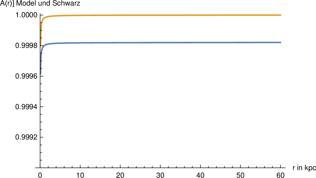
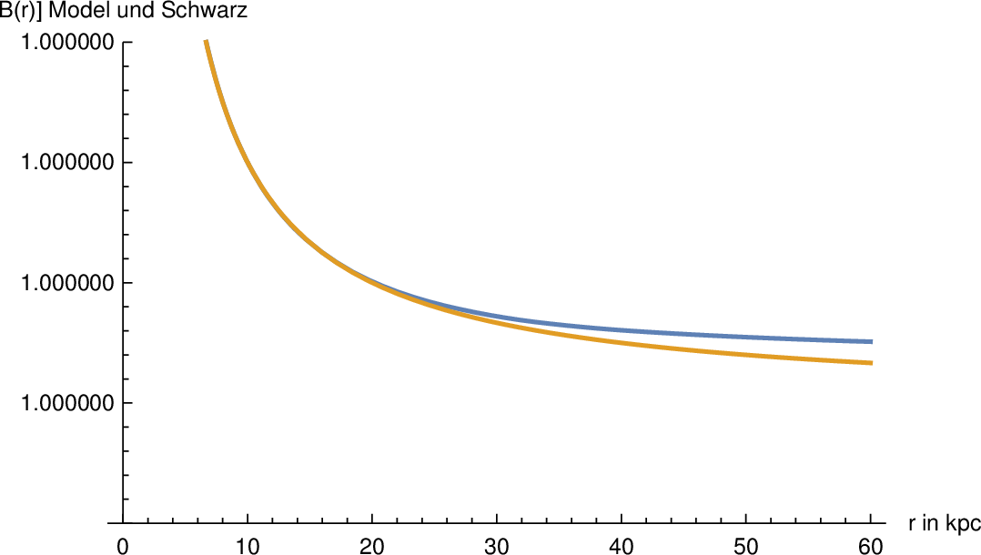
Figure 2: Comparison of the metric coefficients \(a(r)\) and \(b(r)\) for the numerical relativistic model (blue) and the Schwarzschild solution (yellow) for a typical galaxy (\(m \sim 10^{11}M_{\odot}\))..
We can now compare the acceleration 61 of the numerical solution of the relativistic model with a usual MOND model with the simple interpolation function of 50 for \(n=1\),24 \[\mu_M(x)=\frac{x}{1+x} \,, \qquad \nu_M(y)= \frac{1}{2} \big(1 + \sqrt{1+ \frac{4}{y}} \big) \, .\] The radial acceleration of the relativistic model deviates from the classical MOND model for \(r< 35\, kpc\) and coincides with it beyond this radius (figure 3).

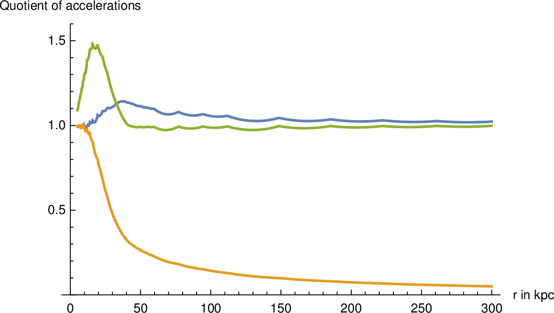
Figure 3: Left: Radial accelerations in \(cms^{-2}\) for galaxies (\(M=10^{-5}\, kpc\)) for the numerical model \(a_{rel}(r)\) (blue), classical MOND \(a_M\) (green), and Schwarzschild-Newton dynamics (yellow). Right: Quotient of model accelerations \(a_X/a_{rel}\), with \(a_{rel}\) the relativistic model, \(X\)=Newton-Milgrom approximation of relativistic model (blue), \(X=\) classical MOND (green), \(X=\) Schwarzschild/Newton (yellow)..
For \(r\leq 15\, kpc\) the model acceleration is at first identical, later still close to the Schwarzschild acceleration; it supersedes the latter increasingly for larger \(r\). For \(r \geq 30\, kpc\)) it is not far from the MOND acceleration \(a_M\) with the “simple” interpolation function. Figure 3, left, shows that for \(r \leq 30\, kpc\) the acceleration of the relativistic model is slightly below \(a_M\); later it approaches \(a_M(r)\) increasingly close (both approximate the deep MOND relation). Figure 5, right, displays the radial accelerations of the Newton-Milgrom approximation \(a_{M}\) (blue), the simple MOND model (green), and the Schwarzschild acceleration \(a_{schw}\) (yellow), effectively identical with the Newton acceleration, all of them divided by \(a_{rel}\).
According to 58 the mass-energy density of the scalar field is here \[\rho_m^{(\phi)} = (8\pi \varkappa)^{-1} c^{-2} \,(2-a ))\Box(g)\sigma \sim \frac{c_1}{r^2} \,, \label{eq32energy32density32phi32central32symmetric}\tag{63}\] the density of the Newtonian mass equivalent 36 twice as much, \(\rho_N^{(\phi)}= 2 \rho_m^{(\phi)}\). Both follow an inverse square law.
4.2 Schwarzschild solution in the inner region↩︎
Using the flat space Milgrom approximation \(a_{\mathsf{rad}}^{(\phi)}(r)= \frac{c^2}{r}\,\sqrt{M\, a_1}\) the boundaries of the transition interval 39 can now expressed in terms of radial distances \[r_0 \leq r \leq r_1 \qquad with r_0, \, r_1 such thata_{\mathsf{rad}}^{(\phi)}(r_0) =\beta\, \mathfrak{a}_0\, , \; a_{\mathsf{rad}}^{(\phi)}(r_1) = \alpha\, \mathfrak{a}_0\]
For radial distances below \(r_0\) the equation 15 reduces to the classical Einstein vacuum equation, its solution to the Schwarzschild metric with central mass \(M\). For distances above \(r_1\) the Milgrom regime dynamics prevails. For the round galaxy model of the last subsection the transition region is (approximately) given by \[5\, kpc \; \leq \; r \, \leq \; 15\, kpc \, .\]
At the level of stellar masses, e.g. for the solar system with \(M \approx 1.97\, AU\) (corresponding to \(m=1\, M_{\odot}\)), the transition region is similarly \[2300 \, AU \, \leq \, r \, \leq \, 7000 \, AU \approx 0.03\, pc\, .\]
The Milgrom regime for a star of solar mass starts at about \(r \sim 7000\, AU\), while for radial distances below roughly \(2.3 \cdot10^3\, AU\) the scalar field is inert (non-dynamical) and the gravitational dynamics is given by the Schwarzschild solution. This shows that our planetary system lies deeply inside the Einstein regime. In particular Einstein’s calculation of the Mercury perihelion advance remains unchanged.
5 Galaxies↩︎
Galaxies have a more complicated shape than the spherically symmetric model considered in the last section. For elliptical galaxies the “round” model may be used for an overall estimates of the scalar field halo, and even for a flat disk the halo far away from the disk is sufficiently round for taking the central symmetric model as a first approximation for the estimate of its total energy content.25. Before discussing this let us first shed a glance at empirically well researched constellations: the radial acceleration relation supported by observational data for a large number of galaxies and at the Milky Way.
5.1 Radial acceleration relation of galaxies↩︎
In this subsection the symbol \(a\) will be used for the modulus of the total radial acceleration in galaxies, \(a_{bar}\) stands for the (Newtonian) radial acceleration \(|a^{(bar)}|\) due to baryonic matter. It is an interesting empirical observation that the dependence of the total acceleration \(a\) on \(a_{bar}\) for galactic rotation curves does not essentially depend on the type or the size of the galaxy McGaugh-et-al:2016?. Over a large range of galactic sizes the dependence is given by a “universal” function \(a_{bar} \mapsto a(a_{bar})\) (universal in the sense of independence of the galaxy studied). This is a rigid empirical constraint for dark matter halos and also constrains the interpolation function \(\tilde{\nu}\), respectively \(\nu\) 47 . In the MOND literature it is called the radial acceleration relation.
In a detailed empirical study of 2700 data pairs \((a_{bar},a)\) for 153 galaxies McGaugh and colleagues established the following empirical fit \(a_{emp}\) of this function : \[a_{emp}(a_{bar}) = a_{bar}\big(1- e^{-\sqrt{\frac{a_{bar}}{\mathfrak{a}_0}}} \big)^{-1} \qquad resp. \quad \tilde{\nu}_{emp}(y)= y\, \big(1-e^{-\sqrt{y}} \big)^{-1} \quad for \; y=\frac{a_N}{a_0}\, .\] The series expansion in the variable \(z=\sqrt{y}\) about \(z_0=0\) up to order 3 \[\nu_{emp}(y)= \sqrt{y} + \frac{1}{2}y + \frac{1}{12}y^{\frac{3}{2}} + \mathcal{O}(\sqrt{y}^4) \, .\] After multiplying with \(a_0\) this empirical fit boils down to the approximation \[\nu_{emp}(a_{bar}) = \sqrt{\mathfrak{a}_0\,a_{bar}} + \frac{1}{2}a_{bar} + \ldots \, . \label{eq32rar32emp32order323}\tag{64}\] In the Milgrom regime this differs from our 54 essentially in the factor \(\frac{1}{2}\) in front of \(a_{bar}\).26 The difference between the two relations may be inspected in figure 4; it does not matter deeper inside the Milgrom regime but seems to be of empirical relevance in the transition region and the beginning of the Milgrom regime (\(3 \, \mathfrak{a}_0 \, > \, a_{bar} > \, 0.1\,\mathfrak{a}_0\)), see figure 4. It seems to be important for the the rotational velocities in the Milky Way (see subsections 5.2, 6.4).

5.2 Rotational velocities in the Milky Way↩︎
Particularly detailed observational data are provided for our own galaxy by Ou et al. Ou-et-al:2023?. It has been claimed in Chan-et-al:2023? that these observations “almost rule out the MOND phenomenology”. This is, however, not the case for the present model (and thus not for MOND phenomenology in general).27
The authors of Ou-et-al:2023? introduce an elaborate model of baryonic matter in the Milky Way, made up from 6 components. For the star mass they combine a bulge model and a disk model, they add two dust components (cold and warm) and two gas components (molecular \(H_2\) and atomic \(H_1\)).28 The resulting Newtonian accelerations induced by each of the components and of the total baryonic mass are given in Ou-et-al:2023? (the total baryonic velocities are shown in the figure below, orange). This allows them to calculate the radial accelerations \(a_{bar}(r)\) in the disk plane and circular velocities \(V_{bar}(r)\) expected from the baryonic matter alone. Finally they fit the dark matter which is needed to fill the gap to 37 data points \(v_{obs}(r_j)\), \((1\leq j \leq 37)\) of observed circular velocities (black in the figure below) with two dark matter models (Einasto profile and NFW profile).29
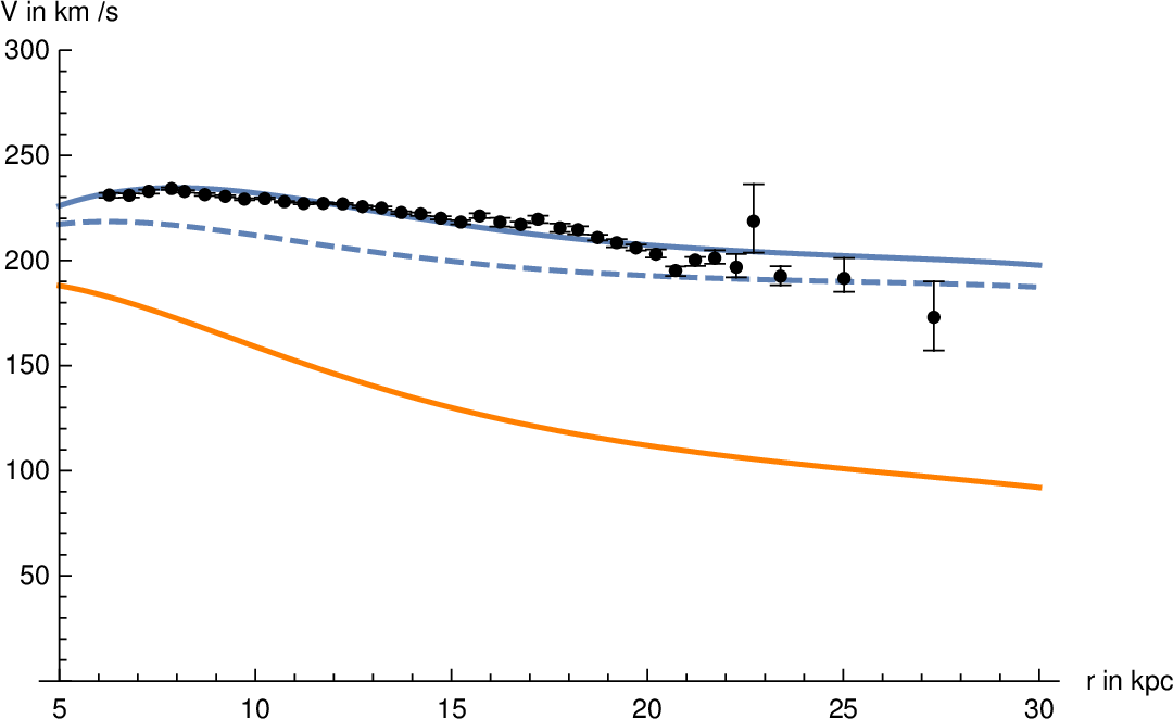
The radial velocities \(V_M\) expected in any MOND approach with interpolation function \(\nu\) are easily derived from these data: \[V_M(r)= \sqrt{ \nu\Big(\frac{V_{bar}(r)}{\mathfrak{a}_0 r}\Big) }\, V_{bar}(r) \,\]
An evaluation of our scalar field model in the flat space Milgrom approximation with \(\nu(x) = \nu_{\mathsf{sf}}(x)\) like in 52 is depicted in figure 5, blue.30 It shows a surprisingly good agreement with the observational data, in particular compared with other MOND functions. The fit is better than for the interpolation function \(\nu_{emp}(y)\) of McGaugh et al. mentioned in the last subsection and much better than for the standard interpolation functions.31
5.3 Scalar field halo in galactic environments↩︎
For approximately round galaxies the energy density falls off with the inverse square of the central distance 63 . In sufficiently large distances this is also the case for disk galaxies32 and results in an approximately linear growth of the integrated mass-energy content \(M_e^{(\phi)}\) and the Newtonian mass equivalent \(M_N^{(\phi)}\), \[M_e^{(\phi)}(R) \approx 4 \pi \int_{0}^{R} u^2\, \rho_m^{(\phi)}(u)\, du \, , \qquad M_N^{(\phi)}(R) \approx 4 \pi \int_{0}^{R} u^2\, \rho_N^{(\phi)}(u)\, du \, .\]
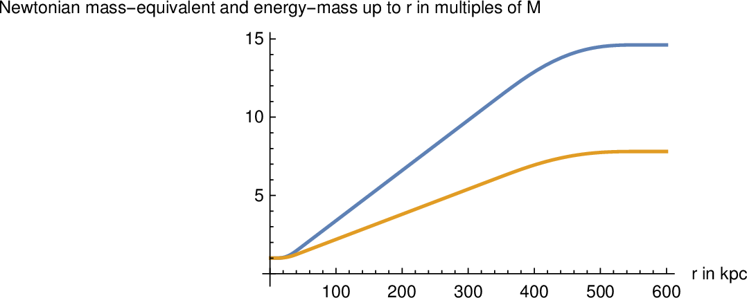
An estimate for the spherical case studied in section 4.1, here with typical distances and mass of galaxies, can be inspected in figure 6. Its total Newtonian mass equivalent up to \(500\, kpc\) is about 15 times the central mass \(M\) of the galaxy and about 6 times \(M\) at \(200\, kpc\). This is quite considerable and has to be taken into account for the study of cluster dynamics, even in the light of the embedding gravitational field of the cluster gas.
6 Open problems↩︎
As for any new approach a series of problems remain open for the scalar field model. Here we discuss four of them: gravitational light deflection, galaxy clusters, cosmology, and general criticism of models with MOND-like dynamics.
6.1 Light deflection↩︎
A particular important application of the reverse Milgrom approximation is the approximative calculation of light deflection in a gravitational field. The calculation for the standard Newton approximation of pressure-free matter given, e.g., in Straumann:GR2004? has to be modified in the Milgrom regime because of the pressure terms of scalar field. In this subsection we simply set \(c=1\).
For a quasi-static metric in a spacetime \(T\times S\) with spatial factor \(S\), \[g_{0j}=0\, , \quad \partial_t g_{\mu\nu}= 0\, , \qquad and \quad d\sigma^2=g_{jk}dx^j dx^k \qquad (j=1,2,3),\] the Fermat principle \[\delta \int dt = 0= \delta \int (-g_{00})^{\frac{1}{2}} d\sigma\] implies that the paths of light in the spatial projection are geodesics of the “Fermat metric” in \(S\) Straumann:GR2004?:33 \[g^{(F)}= g^{(F)}_{jk} dx^j dx^k\, , \qquad g^{(F)}_{jk} = (- g_{oo})^{-1}g_{jk} \,\]
The perturbation terms \(h_{\mu\nu}\) in the weak field metric 29 \(g_{\mu \nu} = \eta_{\mu \nu} + h_{\mu \nu}\) may be slightly rewritten by introducing \[\gamma_{\mu\nu} = h_{\mu \nu} - \frac{1}{2}h \,\eta_{\mu\nu}, \qquad \quad (h= h_{\nu}^{\nu})\] and vice versa \[h_{\mu\nu}= \gamma_{\mu\nu} - \frac{ 1}{2} \gamma\, \eta_{\mu\nu} \qquad \quad (\gamma= \gamma_{\nu}^{\nu}) \, .\] The weak field Einstein equation, up to 1st order, is then Straumann:GR2004?, \[\Box\, \gamma_{\mu\nu} - \eta_{\mu\nu}\partial^{\alpha}\partial^{\beta}\gamma_{\alpha\beta}+ \partial^{\alpha}\partial_{\nu}\gamma_{\mu\alpha} + \partial^{\alpha}\partial_{\mu}\gamma_{\nu\alpha} = 16 \pi G \, T_{\mu\nu}\, .\] With respect to the Hilbert gauge with \(\partial_{\beta}\gamma^{\alpha\beta}= 0\) (which always exist for small perturbations of the Minkowski metric) this simplifies to \[\Box\, \gamma_{\mu\nu} = - 16 \pi G\, T_{\mu \nu}\,. \label{diff32eq32for32gamma}\tag{65}\] and can be solved by retarded integrals (\(x\in \mathbb{R}^3\)) \[\gamma_{\mu\nu}(x^0,x) = 4 G\, \int_{y\in\mathbb{R}^3} |x-y|^{-1}\, T_{\mu\nu}(x^0-|x-y|, y)\,dy \, .\] In the standard Newton case with a pressure free matter source this implies \[\gamma_{00} = 4G\, \int |x-y|^{-1} T_{00}(t,y)\, dy\,, \qquad \gamma_{jj}= 0 \, .\] and because of \(\gamma= - \gamma_{00}\) \[h_{00}= \frac{1}{2}\gamma_{00}\,, \qquad h_{jj}= \frac{1}{2}\gamma_{00}\, .\] A comparison of the Poisson equation for the Newton potential of pressure free matter \(\nabla^2 \Phi_N = 4 \pi G\, T_{00}\) with 65 shows that \(\gamma_{00} = - 4 \Phi_N \,\) thus \(h_{00}=-2\Phi_N, \, h_{jj}= -2\Phi_N\), i.e., \[g = - (1+2\Phi_N)dt^2 + (1-2\Phi_N)\sum_j dx_j^2 \,, \qquad g^{(F)}= \frac{1-2\Phi_N}{1+2\Phi_N} \sum_j dx_j^2 , \label{eq32g32standard32Newton32approximation}\tag{66}\] where \(g^{(F)} \approx (1-4 \Phi_N) \sum dx_j^2\) is the Fermat metric.34
The pressure terms of the scalar field energy tensor, even in baryonic vacuum, make the situation more involved. From 23 and 65 we get \[\Box \gamma_{\mu\nu} = - 2 \big(\Box(g)\sigma (g_{\mu\nu} + 2 A_{\mu}A_{\nu})- 2 \nabla(g)_{(\mu} \partial_{\nu)}\sigma \big)\, . \label{eq32Box32gamma32sf32model}\tag{67}\] In the quasi-static case with flat metric (\(\Box = \nabla^2\)) this is at first order: \[\nabla^2 \gamma_{\mu\nu} = - 2 \big(\nabla^2\sigma (\eta_{\mu\nu} + 2 A_{\mu}A_{\nu})- 2 \nabla_{(\mu} \partial_{\nu)}\sigma \big) \, \label{eq32gamma32quasi32static}\tag{68}\] For the energy component \(\nabla^2 \gamma_{00} = - 2 \nabla^2\sigma\); with 37 (remember \(c=1\) in this subsection) \[\nabla^2 \gamma_{00}= - 2 \nabla^2 \Phi^{(\phi)}\, \qquad and \quad \gamma_{00} = - 2\Phi^{(\phi)}\, .\] 67 implies \(\Box \gamma = 0\). Ignoring solutions of the wave equation we conclude \[\gamma=\gamma_{\nu}^{\nu} = 0 \, , \qquad\quad h_{\mu \nu}= \gamma_{\mu\nu}\, . \label{eq32h32and32gamma}\tag{69}\] All in all \[h_{00} = - 2\Phi^{(\phi)}\;\qquad and \quad \nabla^2\,h_{jj} = - 2 \big(\nabla^2 \sigma - 2 \nabla_j\partial_j \sigma \big) \, . \label{eq32hjj32scalar32field}\tag{70}\]
This result is considerably more involved than for pressure free (“ordinary”) matter. Only the time component of the metric perturbation behaves like in the ordinary matter case. The spatial diagonal perturbations are modified by second order partial derivatives and depend on the spatial constellation of the scalar field
In the centrally symmetric case (section 4) with the Minkowski metric in spherical polar coordinates \[\widetilde{\eta} = \mathtt{diag}(-1,\,1,\, r^2,\, r^2 \sin^2 \vartheta) \, , \qquad (x^0, x^1,x^2,x^3)= (t, r,\vartheta,\phi) ,\] and its perturbation \[g= \mathtt{diag}(-1+h_{00},\,1+h_{11},\, r^2,\, r^2 \sin^2 \vartheta)\,\] the Milgrom equation is solved by \(\sigma \approx c_1 \ln r\). This follows from 57 which is at first order \[\sigma' = A^{-\frac{1}{4}}B^{\frac{1}{2}}\, \frac{c_1}{r} \underset{1}{=} (1+\frac{1}{4}h_{00}+ \frac{1}{2}h_{11})\, \frac{c_1}{r} \underset{1}{=} \frac{c_1}{r} \, .\] In this case \[\Delta \sigma = \sigma''+\frac{2}{r}\sigma' = \frac{c_1}{r^2} =- \sigma'' \qquad and \quad \nabla_1\partial_1\sigma= \sigma'' = - \Delta \sigma\, .\]
From 70 \[\Delta h_{11} = - 2 (\Delta \sigma - 2 \nabla_1\partial_1 \sigma)= -6 \,\Delta \sigma = -6\, \Phi^{(\phi)}\,.\]
The metric with perturbation from the scalar field only is \[- (1 +2 \Phi^{(\phi)})dt^2 + (1-6\Phi^{(\phi)})\Big( dr^2 + r^2 \big(d\vartheta^2 + \sin^2\vartheta\, d\phi^2 ) \Big)\, .\] Adding the effects of the baryonic mass, the perturbed metric becomes \[g = - (1 + 2 \Phi^{(bar)} + 2\Phi^{(\phi)})dt^2 + (1-2\Phi^{(bar)} -6\Phi^{(\phi)})\Big( dr^2 + r^2 \big(d\vartheta^2 + \sin^2 \vartheta\, d\phi^2 )\Big) \label{eq32perturbed32metric32centr32symm}\tag{71}\] and the Fermat metric \[g^{(F)} = \frac{1-2\Phi^{(bar)} -6\Phi^{(\phi)}}{1 + 2 \Phi^{(bar)} + 2\Phi^{(\phi)}} \Big( dr^2 + r^2 \big(d\vartheta^2 + \sin^2 \vartheta\, d\phi^2)\Big) \, .\] At first order in the potentials \[g^{(F)} \approx \big(1- 2(2\Phi^{(bar)} + 4 \Phi^{(\phi)})\big)\,\Big( dr^2 + r^2 \big(d\vartheta^2 + \sin^2 \vartheta\, d\phi^2) \Big)\, .\] This corresponds to a refraction index \(1-(2\Phi^{(bar)}+4\Phi^{(\phi)})\).
In the centrally symmetric case the scalar field potential contributes twice as much as one would expect from an equally large potential of (pressure free) baryonic matter in relativistic calculations.35 In the MOND literature it is often assumed that the gravitational light deflection can be calculated from the phantom matter distribution like for pressure free matter (including the general relativistic factor 2) Famaey/McGaugh:MOND?; but its derivation remains often opaque. The deviation of our model from the default assumption in MOND ought to have observable consequences. These remain to be checked and generalization, most importantly to the axis symmetric case, have to be studied.
6.2 Galaxy Clusters↩︎
The dynamics of galaxy clusters is a challenge for dark matter theories and an unsolved problem for MOND Sanders:2003?. For a first exploration of the scalar field approach to galaxy clusters we use the simplifying assumption of centrally symmetric shapes for the baryonic mass-density of the hot gas and the star mass, like in model calculations in the astronomical literature Reiprich:Diss?, Sanders:2003?. Given the density functions for the hot gas \(\rho^{(g)}\) and the stellar content \(\rho^{(\ast)}\), the respective baryonic masses \(M^{(g)}\) and \(M^{(\ast)}\) up to the central distance \(r\), the Newtonian central accelerations \(a^{(g,N)}, a^{(\ast,N)}\) and the total Newtonian acceleration due to baryonic sources \(a^{(bar)}= a^{(g,N)} + a^{(\ast,N)}\) are easily to be calculated, of course all of them in dependence of \(r\).
The hot gas component of the baryonic mass in galaxy clusters may be considered s a smoothly changing external medium \(S_g\) for the motion of individual galaxies \(S_j\) \((1\leq j \leq N,\; N\) the number of galaxies) or, alternatively, for the whole collection of galaxies \(S_{\ast} = \bigcup_j S_j\). The reference system for a Newton approximation of the field about each individual galaxy \(S_j\) has to be centred on the barycentre of \(S_j\). Every galaxy \(S_j\) is falling freely in the gravitational field induced by \(S_g\) and \(\bigcup_{k \neq j} S_k\). We consider the following alternative assumptions for the flat space Newton-Milgrom approximations of the field around each galaxy in such a weakly binding external system:
The hot gas mass dominates the linear approximation in the cluster barycentric rest system and overlays the scalar field formation of the galaxies \(S_j\).
The hot gas induces a scalar field halo in the cluster barycentric system. Because of the free fall of the galaxies the scalar field density of each of them 46 may be determined in the Newton-Milgrom approximation centred on \(S_j\) and is exclusively induced by the baryonic matter of \(S_j\). The effects of the external baryonic masses (gas and the other) are shielded away by the galaxy’s free fall.
Case (A) corresponds to the viewpoint of the external effect (EFE) in classical MOND. Inside galaxies it is considered as empirically well supported for the motion of stars with the corresponding galaxies as their external systems Chae-McGaugh-et-al:2020?, Kroupa-et-al:2024Star-clusters?. In MOND it is treated as a principle and assumed to hold also for the motion of galaxies in galaxy clusters. In the present framework this is not mandatory.36 It even seems to be undermined by the empirical data for cluster dynamics (see below).
In case (A) one may work with the continuous density models \(\rho^{(g)}\) and \(\rho^{(\ast)}\) of both baryonic mass sources, gaseous and stellar. They induce scalar field halos satisfying 42 , respectively 43 . The accelerations due to the scalar field (here denoted as \(a^{(\ldots, \mathtt{sf})}\)) are then:
- \[a^{(g,\mathtt{sf})} = h \, \sqrt{\frac{\mathfrak{a_0}}{|a^{(bar)}|}} a^{(g,N)} , \; \qquad a^{(\ast,\mathtt{sf})} = h \,\sqrt{ \frac{\mathfrak{a}_0}{|a^{(bar)}|} }\, a^{(\ast,N)}\, \qquad \big( h= h(|a^{(bar)}|,\tilde{\alpha},\tilde{\beta}) \big)\]
The total scalar field acceleration \(a^{(\mathtt{sf})}\) is additively composed, \[a^{(\mathtt{sf})} = h\,\sqrt{ \frac{\mathfrak{a}_0}{|a^{(bar)}|} }\, a^{(bar)} = a^{(g,\mathtt{sf})} + a^{(\ast,\mathtt{sf})} \, .\] Under the assumption of central symmetry the accelerations can be straightforwardly converted into respective mass expressions \(M^{(\mathtt{sf})}, M^{(g,\mathtt{sf})}, M ^{(\ast,\mathtt{sf})}\) (\(M= r^2\,G_N^{-1}\, a\)) and vice versa.
The bulk of baryonic matter given by the gas mass is often approximated by a \(\beta\) model.37 The Newtonian mass \(M^{(g,N)}\) and acceleration \(a^{(g,N)}\) induce a scalar field halo according to 42 , respectively 43 with acceleration \(a^{(g,\mathtt{sf})}\) and Newtonian mass equivalent \(M^{(g,\mathtt{sf})}\). The distribution of the star mass is less regular. Its empirical determination is difficult; reliable values are given in the literature at specific distances only, e.g. for \(r_{500}\).38
In the case (B) the scalar field halo of the gas can be computed like above (A’). On the other hand, the acceleration induced by the scalar field of the galaxies in a continuity model for the star mas \(\rho^{(\ast)}\) lies in the Milgrom regime and is given by
- \[a^{(\ast,\mathtt{sf})} = \sqrt{ \frac{\mathfrak{a}_0}{|a^{(\ast,N)}|} \big)}\, a^{(\ast,N)} \, .\]
It is not easy to decide between (A) and (B) on the theoretical level; we therefore check the alternatives against the empirical data for a typical cluster, say Coma.
Let \(M_{500}^{(tot,N)}\) denotes the total dynamical mass of the cluster at the radius \(r_{500}\), determined in Newton gravity, \(M^{(gas)}_{500}\) the mass of the hot gas, \(M^{(\ast)}_{500}\) the estimated luminous mass of stars/galaxies and \(M_{500}^{(bar)}= M^{(gas)}_{500}+M^{(\ast)}_{500}\). In Reiprich/Zhang_ea:Corr? we find for Coma in units of \(10^{13}\, M_{\odot}\) \[M_{500}^{(tot)} = 65.5 \pm 7.9\, , \quad M^{(gas)}_{500} = 8.42 \pm 0.63\, , \quad M^{(\ast)}_{500} =1.31 \pm 0.18 \, , \label{eq32parameters32Coma}\tag{72}\] with \(r_{500} \approx 1.278\, Mpc\) according to Reiprich:Diss?.39
The missing mass in Newtonian gravity \[\Delta M^{(N)}_{500} = M_{500}^{(tot)} - M_{500}^{(bar)} \approx 56 \cdot10^{13}\,M_{\odot} \,\] is often understood as the amount of dark matter up to this radius.40
The scalar field contributions to the accelerations at \(r_{500}\) are far below \(\mathfrak{a_0}\), in units of \(10^{-8}\, cm\, s^{-2}\)
| Case | \(a^{(g,\mathtt{sf})}\) | \(a^{(\ast,\mathtt{sf})}\) | \(a^{(\mathtt{sf})}\) | |||
|---|---|---|---|---|---|---|
| (A) | 0.315 | 0.043 | 0.358 | |||
| (B) | 0.315 | 0.116 | 0.431 |
The associated Newtonian mass equivalents of the scalar field \(M^{(g,\mathtt{sf})}, \,M^{(\ast,\mathtt{sf})}\), \(M^{(\mathtt{sf})}= M^{(g,\mathtt{sf})}, + M^{(\ast,\mathtt{sf})}\) and the missing masses of the present approach, \[\Delta M^{(\mathtt{sf})}_{500} = M_{500}^{(tot)} - ( M_{500}^{(bar)} + M_{500}^{(\mathtt{sf})} ) \, ,\] can be derived from this. Their values are given in the following table in \(10^{13} M_{\odot}\).41
| Case | \(M^{(g,\mathtt{sf})}\) | \(M^{(\ast,\mathtt{sf})}\) | \(M^{(\mathtt{sf})}\) | \(M^{(\mathtt{bar})}\) | \(M^{(\mathtt{bar})} + M^{(\mathtt{sf})}\) | \(\Delta M^{(\mathtt{sf})}\) | |||
|---|---|---|---|---|---|---|---|---|---|
| (A) | 37.0 | 5.0 | 42.0 | 9.7 | 51.7 | 13.8 | |||
| (B) | 37.0 | 13.6 | 50.6 | 9.7 | 60.3 | 5.2 |
This is an interesting result. Already the missing mass of case (A) is less than half the missing mass of classical MOND calculations. Assuming MOND dynamics R. Sanders arrived for Coma at an unexplained residuum \(\Delta M^{\mathtt{M}}_{500} \approx 30\cdot 10^{13} M_{\odot}\) Sanders:2003?. It led him to the hypothesis of an additional component of dark matter (probably made up of sterile neutrinos).
Case (B) looks even better. The missing mass \(\Delta M^{(\mathtt{sf})} = 5.2\cdot 10^{13} M_{\odot}\) for the central values of 72 lies inside the empirical error interval. This speaks strongly in favour of the hypothesis (B). The result has to be checked seriously for more galaxies, but that cannot be done here.42
6.3 Cosmology↩︎
Large scale cosmological models of the present approach lie in the Einstein regime of the scalar field. This may be considered a weak spot or an advantage, depending on the scientific perspective taken. In the light of the growing difficulties of the actual standard model of cosmology it appears at least dissatisfying that our Lagrangian 5 does not endow the scalar field with a dynamical role at the cosmological level. Modifications and improvements may be looked for.
6.4 Criticism of MOND in general↩︎
Many criticism of MOND in general have been brought forward in the literature. Some of it (lacking connection to general relativity, indecision whether it modifies dynamics or gravity etc.) become pointless in the present approach. Others do still apply, most importantly among them, the non-fundamentality of the approach. This deficiency may perhaps be relaxed in case the Weyl geometric gravity approach in Ghilencea:2019JHEP?, Ghilencea:2022SMWeyl?, Ghilencea/Harko:2021?, Ghilencea:2023?, Ghilencea:2025?, Burikham/Harko-ea:2023? progresses and turns out helpful for a program of integrating gravity with quantization,43 and if the link of the model to the latter can be consolidated.
Moreover, in the paper Chan-et-al:2023? the authors claim empirical inadequacy of MOND at the level of galaxy dynamics, the very range on which the latter boasts its main success. They analyse the recent data of rotation velocities measured in the Milky Way Ou-et-al:2023? from a classical MOND perspective, with regard to two families of interpolation functions, the algebraic one of 50 and an analytic one considered in Famaey/McGaugh:MOND?, \[\nu_{\delta}(y)= \Big(1- e^{-\frac{\delta}{2}} \Big)^{-\frac{1}{\delta}}\, .\] The authors argue that with both types of interpolation functions the effective total accelerations calculated in MOND are incompatible with the observational data of Ou-et-al:2023?. They draw the conclusion that this “can almost rule out MOND phenomenology” in general.
In subsection 5.2 we have shown that this is not the case for the present approach. As the interpolation functions of the flat space Milgrom approximation satisfy the defining conditions 48 of a MOND algorithm the generalization of the authors is premature. Moreover, even for classical MOND the argument of the authors of Chan-et-al:2023? is not impeccable. They derive their inconsistency result on the basis of a comparably simple baryonic mass model for the Milky Way with two components only, composing a bulge model with a flat disk, rather than the elaborate model used by the authors of Ou-et-al:2023?. This is problematic, as the effective total acceleration of any MOND model is highly sensitive to variation of the Newtonian acceleration of the baryonic mass.
But even using the baryonic mass distribution of Chan-et-al:2023? the standard interpolation functions do not lead to an acceptable reproduction of the observational data.
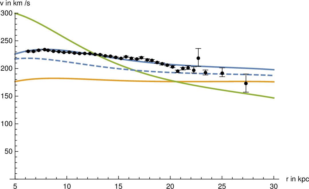
In this sense, the remarks of Chan et al. hint to an important observational domain (rotation curves of the Milky Way with baryonic accelerations close to the critical value \(\mathfrak{a_0}\)) for which the present model outmatches the two families of MOND interpolation functions mentioned above. This has to be checked further.
7 Resumée and discussion↩︎
Already at the theoretical level we have found interesting properties of the scalar field introduced in this paper (section 2.1). First and above all, it has been shown that a single gravitationally coupled scalar field is able to generate MOND-typical free fall trajectories in the flat approximation and is accompanied by gravitational light bending resembling the one expected in a dark matter approach or in ordinary MOND, although not identical with it. This is no triviality; earlier approaches to relativistic generalizations of MOND have postulated quite involved structures, often with two basically unrelated Riemannian metrics and diverse additional fields (section 1.2). In the present approach the metrical generalization of Riemannian geometry is achieved by the weakest possible variant of Weyl geometry: the integrable case, with the Einstein gauge (frame) specifying physical measurements. On the one hand, the scalar field is part and parcel of the Weyl geometric modification of Riemannian geometry, i.e., of the gravitational structure. On the other side its energy-momentum tensor entails an important addition to the right hand side of the Einstein equation, letting it appear as a peculiar type of dark matter (with unexpected pressures). In this sense it fits seamlessly into the persepctive of Lehmkuhl/Martens:2020?. For strong gradients the scalar field is screened away (Einstein-Newton regime); only for weak gradients the scalar field modifies Einstein-Newton gravity (Milgrom regime).
For the central symmetric case these effects can be quantitatively investigated by numerical calculations showing how the Schwarzschild metric is deformed in the Milgrom regime, and how the energy and Newtonian mass equivalent of the scalar field add up in the long range (section 4.1).
In the flat space approximation the general relativistic dynamical equation of the scalar field specializes to the non-linear Poisson equation known from MOND (deep MOND case), and the Newton approximation of the Einstein equation acquires a non-negligible source term due to the scalar field in addition to the baryonic sources (section 3). The flat approximation can be used to infer backwards crucial properties of the scalar field, in particular those relating to the energy-momentum tensor. In the Milgrom regime the present model has precisely determined “interpolation” functions in the sense of the MOND approach, which facilitate a quantitative comparison with other MOND models (section 3.3).
At the galactic level the radial acceleration function implied by the interpolation functions of the present model is close to the one empirically determined by McGaugh et al. McGaugh-et-al:2016?. Relevant differences may arise close to the critical acceleration for MOND \(\mathfrak{a_0}\) (section 5.1). Observational data on radial velocities in the Milky Way give precise data on this acceleration regime Ou-et-al:2023?. Starting from the data given there on the baryonic matter distribution in the Milky Way the scalar field model predicts the total accelerations and the radial velocities surprisingly well (section 5.2, 6.4). Moreover, for galaxy clusters it may even make a crucial difference to the classical MOND calculations: If one adds the Newtonian mass equivalent of the scalar field halos of the freely falling galaxies to that of the hot gas mass, the total dynamic mass of the model seems to suffice for explaining the observational data; at least this is so for Coma (section 6.2).
A major open problem results from the pressure term of scalar field energy tensor. It has strong repercussions on the gravitational light deflection expected in the model. The contribution of the scalar field to the refraction index differs from the one
expected for classical MOND. In the centrally symmetric case it is twice the one expected there and for cold dark matter (section 6.1). This should allow to discriminate between the approaches. If the
present model fails in this point it will be empirically refuted; the theoretical contributions mentioned above would then remain the only achievements of the approach.
Acknowledgements: I thank P. Kroupa for comments on an earlier version of this paper. An anonymous referee made me aware of the importance of Ou-et-al:2023?, Chan-et-al:2023?.
8 Appendix↩︎
8.1 Short outline of Weyl geometric methods and the notation used↩︎
A Weylian metric may be characterized by an equivalence class of pairs \([(g,\varphi)]\) consisting of a semi-Riemannian metric \(g=g_{\mu\nu} dx^{\mu}dx^{\nu}\), the Riemannian component of the Weylian metric, and an associated 1-form \(\varphi= \varphi_{\nu}dx^{\nu}\) representing a scale connection. Equivalences arise from point dependent rescalings of the Riemannian component by a positive function \(\Omega(x)\), \[\tilde{g}= \Omega^2 g \, ,\] and an associated gauge transformation of the 1-form, \[\tilde{\varphi}= \varphi- d \log \Omega \qquad (\log = \ln) \, .\] Choosing a representative \((g,\varphi)\) of the class is the same as gauging the Weylian metric. The latter has a unique compatible scale invariant affine connection \(\Gamma\) with an associated covariant derivative \(\nabla = \nabla(\Gamma)\). One may write the Weylian affine connection and its covariant derivative of a vector field \(X\) in the form \[\Gamma = \Gamma(g) + \Gamma(\varphi) \qquad respectively \qquad \nabla {\nu} X^{\mu } = \partial_{\nu}X^{\mu}+ \Gamma_{\nu \lambda}^{\mu}X^{\lambda} \label{eq32decomposition32affine32connection}\tag{73}\] where \(\Gamma(g)\) denotes the Levi-Civita connection of \(g\) and \(\nabla(g)\) the associated covariant derivative. \(\Gamma(\varphi)\) is an expression (not a connection but a tensor) codifying the contribution of \(\varphi\) to the scale invariant affine connection. Sometimes \(\Gamma\) is written as \(\Gamma(g,\varphi)\) for emphasizing the combination of the gauge dependent contributions, although this hides its gauge independence.
For a scale covariant field \(X\) of (Weyl-) weight \(w\) transforming under rescaling by \(\tilde{X}= \Omega^w X\) \(\nabla X\) is not scale covariant, while \[D_{\nu} X = \nabla(g)_{\nu}X + w \, \varphi_{\nu}\, X \,\] is again scale covariant of the same weight \(w\). \(D\) is called the scale covariant derivative operator. It satisfies the condition \[D_{\nu}g_{\mu\lambda} = 0 \, ;\label{eq32Dg610}\tag{74}\] in other words, it is compatible with the metric in the sense of Weyl geometry.
The curvature tensors \(Riem = Riem(\Gamma)\) (generalized Riemann curvature) and \(Ric(\Gamma)\) (Ricci) derived from the affine connection \(\Gamma\) are scale invariant. In any gauge they can be composed similar to \(\Gamma\), e.g., \(Riem(g) + Riem(\varphi)\) etc. The scalar curvature \(R(g,\varphi)\) depends on the gauge and is scale covariant of weight \(-2\). For more details see appendix 8.3.1 and the classics Weyl:GuE?, Weyl:InfGeo?, Pauli:1921?, Eddington:Relativity?, Dirac:1973?.44
Here we work mostly with Weylian metrics of dimension \(n=4\) and Lorentzian signature \((-+++)\). Moreover, in our context the curvature of the scale connection is assumed to vanish, \[d\varphi = 0 \, ,\] while the structure is enriched by a real valued scale covariant field \(\phi\) of weight \(-1\).
There are two special gauges. One exploits the vanishing of the scale connection, \(\varphi=0\), and characterizes the Weylian metric by its Riemannian component only; this is called the Riemann gauge. Another distinguished gauge is the one in which the scalar field is constant, \(\phi(x)=\phi_0\) (for all \(x\)) and may be called scalar field gauge. As the present model assumes non-minimal coupling of \(\phi\) to gravitation, this gauge has strong analogies to the Einstein frame in JBD theory; accordingly it will also be referred to as the Einstein gauge of the Weylian metric. Matter fields are assumed to break the scale symmetry and to couple with gravity in the Einstein gauge. Thus test matter follows the geodesics of the \(\Gamma(g_E)\) with \(g_E\) the Riemannian component of the Einstein gauged metric. Equalities in these gauges are denoted \(\underset{Rg}{\doteq} \; for the Riemann gauge, \; \underset{Eg}{\doteq} \; for the Einstein gauge.\) In Riemann gauge the scalar field is written in exponential form, \[\phi(x) \underset{Rg}{\doteq} \phi_0 e^{-\sigma(x)}\, . \label{eq32phi32exponential32form}\tag{75}\] Because the transition from Riemann to Einstein gauge is accomplished by rescaling with \(\Omega=e^{-\sigma}\), the scalar field and the scale connection in Einstein gauge are given by \[\phi \underset{Eg}{\doteq} \phi_0 \qquad and \qquad \varphi \underset{Eg}{\doteq} - d \log \Omega = d \sigma \,.\] This shows that the scalar field \(\phi\) and the integrable scale connection \(\varphi\) can be traded against each other. Taken together they represent the scalar field degree of freedom of the model.
No direct physical relevance is assumed in the following for the scale invariant affine connection \(\Gamma\); the Weyl geometric framework is mainly used as a symbolic tool particularly well adapted for forming scale invariant Lagrangians and the derivation of scale covariant dynamical equations. Reference to empirical data will be made via the Einstein gauge. In this sense the present model is placed in a kind of overlap region of JBD theory and Weyl geometric field theory. Even though it uses the latter in a moderate way, it cannot be reduced to JBD theory. The latter confines itself to shifting perspectives in a family of conformally related Riemannian metrics endowed with a rescaling field, but lacks a consistent framework for working with scale covariant derivatives and dynamical equations.
Similar to 73 for the affine connection the curvature quantities of Weyl geometry in any given gauge \((g,\varphi)\) can be composed from a Riemannian component (the respective quantity with regard to \(g\) only) and an additional term due to the scale connection:45
\[\begin{align} Riem(g,\varphi) &=& Riem(g)+ Riem(\varphi)(curvature tensor) \\ G_W = G(g,\varphi) &=& Riem(g,\varphi) - \frac{1}{2}R(g,\varphi )\, g \qquad (Einstein tensor)\\ &=& G(g) + G(\varphi) \\ R(g,\varphi) &=& R(g)+R(\varphi)(scalar curvature) \end{align}\] The first two are scale invariant, while \(R(g,\varphi)\) is scale covariant of weight \(-2\).
Scale connection contributions to Weyl geometric terms in dimension \(n\) are: \[\begin{eqnarray} \Gamma(\varphi)_{\mu \nu}^{\lambda} &=& \delta_{\mu}^{\lambda}\varphi_{\nu} + \delta_{\nu}^{\lambda}\varphi_{\mu} - g_{\mu\nu}\,\varphi^{\lambda} \\ Ric(\varphi)_{\mu \nu} &=& (n-2)\big(\varphi_{\mu}\varphi_{\nu} - \nabla(g)_{(\mu}\varphi_{\nu})\big) -\big((n-2)\varphi_{\lambda}\varphi^{\lambda} + \nabla(g)_{\lambda}\varphi^{\lambda} \big)\, g_{\mu \nu} \\ R(\varphi) &=& - (n-1)(n-2)\varphi_{\lambda}\varphi^{\lambda} - 2(n-1)\nabla(g)_{\lambda}\varphi^{\lambda} \tag{76} \\ G(\varphi)_{\mu \nu} &=& (n-2)\Bigl( \varphi_{\mu} \varphi_{\nu}- \nabla(g)_{(\mu}\varphi_{\nu)} + \big(\frac{1}{2}(n-3)\varphi_{\lambda}\varphi^{\lambda} + \nabla(g)_{\lambda} \varphi^{\lambda} \big)g_{\mu\nu} \Bigr) \tag{77} \\ for n=4: &= & 2 \bigl( \varphi_{\mu} \varphi_{\nu}- \nabla(g)_{(\mu}\varphi_{\nu)} \bigr) + \big(\varphi_{\lambda}\varphi^{\lambda} + 2\nabla(g)_{\lambda} \varphi^{\lambda} \big)g_{\mu\nu} \nonumber \\ &\underset{Eg}{\doteq}& 2 \bigl( d\sigma_{\mu} d\sigma_{\nu}- \nabla(g)_{(\mu}d\sigma_{\nu)} \bigr) + \big(d\sigma_{\lambda}d\sigma^{\lambda} + 2\nabla(g)_{\lambda} d\sigma^{\lambda} \big)g_{\mu\nu} \tag{78} \end{eqnarray}\]
8.2 Variational derivatives↩︎
Variational derivatives of a Lagrangian density \[\mathcal{L} = L \sqrt{|g|}\] with regard to a field \(Y\) are written as Euler expressions denoted by square brackets with lower index
\(Y\), \[[\mathcal{L}]_Y =
\frac{\delta \mathcal{L}}{\delta Y}= \frac{\partial \mathcal{L}_Y}{\partial Y} - \partial_{\nu} \frac{\partial \mathcal{L}_Y}{\partial(\partial_{\nu } Y)} \pm \ldots \, , \,\] with the Euler equation \([\mathcal{L}]_Y
=0\), the dynamical equation for \(Y\).
Variation \(\delta g^{\mu \nu}\)
The variation \([\mathcal{L}_H]\) of the Weyl geometric scalar curvature with a non-minimally coupled scalar field leads to Drechsler/Tann?46 \[[\mathcal{L}_H
]_{g^ {\mu\nu}} = \Big( \frac{(\hbar c)^{-1}}{2} (\xi \phi)^2 G(g,\varphi)_{\mu\nu} + \frac{(\hbar c)^{-1}}{2}\big((D_{\lambda}D^{\lambda}(\xi \phi)^2)\,g_{\mu\nu} - D_{(\mu}D_{\nu)}(\xi\phi)^2 \big) \Big)\,\sqrt{|g|} \, ,
\label{eq32variation32Hilbert32term}\tag{79}\] with the Weyl geometric Einstein tensor \(G(g,\varphi) = Ric(g,\varphi)-\frac{1}{2}R(g,\varphi) g\). The variational derivative 79 contains two contributions not known from the Riemann-Einstein case. One results from \(G(\varphi)\), the contribution of the scale connection to the Weyl geometric curvature
77 , the other one from the non-minimal coupling of the scalar field like in JBD theory Capozziello/Faraoni?, Fujii/Maeda?. Here it appears in a scale covariant form (the
second term on the r.h.s in 79 ). Taken together the second order terms cancel in dimension \(n=4\). In the Einstein gauge they are with 77 ,91 : \[(\xi \phi)^2 G(\varphi)_{\mu \nu} + \big((g_{\mu
\nu}\, D_{\lambda}D^{\lambda}(\xi \phi)^2 - D_{(\mu}D_{\nu)}(\xi\phi)^2 \big) \underset{Eg}{\doteq} (\xi \phi_0)^2 \, \big(3\partial_{\lambda}\sigma \partial^{\lambda}\sigma\, g_{\mu \nu} - 6 \partial_{\mu}\sigma \partial_{\nu}\sigma \big)
\label{eq32G40varphi4132and32additional32term}\tag{80}\]
The variation of all scale invariant Lagrange densities leads to scale invariant expressions with Weyl weight \(-2\) and of physical dimension \(EL^{-1}\) (metrical only in the Einstein gauge).
\[\begin{align} (\hbar c)\sqrt{|g|}^{\,-1} [\mathcal{L}_H]_{g^{\mu \nu}} &=& \frac{(\xi \phi)^2}{2} G(g,\varphi)_{\mu\nu}\, + \frac{1}{2}\big(g_{\mu\nu}\, D_{\lambda}D^{\lambda}(\xi \phi)^2 - D_{(\mu}D_{\nu)}(\xi\phi)^2 \big)\, \nonumber \\ (\hbar c)\sqrt{|g|}^{\,-1} [ \mathcal{L}_{\phi_2} ]_{g^{\mu \nu}} &=& - \frac{\alpha}{2} \xi^2 D_{\mu}\phi D_{\nu}\phi - \frac{1}{2} {L}_{\phi_2} g_{\mu \nu} \label{eq32scale32covariant32Euler32exp32g} \\ (\hbar c)\sqrt{|g|}^{\,-1} [ \mathcal{L}_{\phi_3} ]_{g^{\mu \nu}} &=& - \, s_{\phi}\,\, \frac{\beta}{2} \xi^3 \phi^{-2}|D \phi| \,D_{\mu}\phi \,D_{\nu}\phi - \frac{1}{2} {L}_{\phi_3}\, g_{\mu \nu} \nonumber \\ (\hbar c) \sqrt{|g|}^{\,-1} [ \mathcal{L}_{_2\phi} ]_{g^{\mu\nu}} &=& \xi^2\phi\, \Big( \big( D_{\mu}D_{\nu}\phi - \frac{1}{2}D_{\lambda}D^{\lambda}\phi\,g_{\mu\nu} \big)\,A_{\lambda}A^{\lambda} + D_{\lambda}D^{\lambda}\phi \, A_{\mu}A_{\nu} \Big)\, \nonumber \\ \sqrt{|g|}^{\,-1} [ \mathcal{L}_{V} ]_{g^{\mu \nu}} &=& - \frac{1}{2} {L}_{V} g_{\mu \nu} \nonumber \end{align}\tag{81}\] For baryonic matter we consider the Einstein gauge \[\sqrt{|g|}^{\,-1} [ \mathcal{L}_{m} ]_{g^{\mu \nu}} \underset{Eg}{\doteq} - \frac{1}{2}\, T^{(bar)}_{\mu\nu}\] and introduce a place holder \([ T^{(bar)}]\) in other gauges by formal rescaling (weight \(-2\)) the Einstein gauged energy tensor.
Because of \[tr\, [ \mathcal{L}_{_2\phi} ]_{g^{\mu\nu}}=0\] and \[tr\, [\mathcal{L}_H]_{g} = - \mathcal{L}_H + \frac{3\,(\hbar c)^{-1}}{2}(D_{\lambda}D^{\lambda}(\xi \phi)^2)\,\sqrt{|g|}\, \label{eq32trace32L-H-g}\tag{82}\] twice the trace of the Einstein equation (including the place holder for the baryonic energy tensor) is \[2\, tr\,[{L}]_g = - 2{L}_H + 3\,(\hbar c)^{-1}\xi^2\,D_{\lambda} D^{\lambda}\phi^2 \; - 2{L}_{\phi_2}- {L}_{\phi_3} - 4 {L}_V \; - tr\, [T^{(bar)}]\, . \label{eq32trace32L-g}\tag{83}\]
Variation \(\delta \phi\)
For the variation of the scalar field the scale covariance of the expressions in \(\phi\) (with values in the respective gauge bundles of the scale group) allows to work with the Euler expressions in bundle values, thus
avoiding lengthy calculations in derivatives of \(\sqrt{|g|}\) Frankel:Geometry?: \[[{L}]_{\phi} = \frac{\delta{L}}{\delta \phi} = \frac{\partial{L}}{\partial \phi} - D_{\mu}\frac{\partial{L}}{\partial(D_{\mu}\phi)} + D_{\mu}D_{\nu}\frac{\partial {L}}{\partial(D_{\mu}D_{\nu}\phi)} \pm \ldots\] with the Euler
equation \([{L}]_{\phi} =0\). Similarly the Euler expression of a vector or tensor field \(Y\) without scaling symmetry (like the scale connection \(\varphi\)) can be written as: \[[{L}]_{Y} = \frac{\delta{L}}{\delta Y} = \frac{\partial{L}}{\partial Y} - \nabla(g)_{\mu}\frac{\partial{L}}{\partial(\nabla(g)_{\mu}Y)} \pm \ldots\]
In fact, the Weyl geometric compatibility relation 74 implies \(D_{\lambda}\sqrt{|g|}=0\), just like the Riemannian compatibility implies \(\nabla(g)_{\lambda}\sqrt{|g|}=0\). Because of this (and of course \(\frac{\delta \sqrt{|g|}}{\delta \phi}=0\)) the Euler expressions of \(\delta \phi\) satisfy \([\mathcal{L}_X]_{\phi} = [L_X]_{\phi}\sqrt{|g|} \,\) even for the terms containing derivatives , i.e., \(X\in \{\phi_2, \,\phi_3,\, _2\phi \}\). Therefore \[[\mathcal{L}_X]_{\phi} = 0 \qquad \longleftrightarrow \qquad [L_X]_{\phi} = 0 \,\]
Leaving aside coefficients, i.e., using the simplified expression \[[{\tilde{L}}_{\phi_2}] = - D_{\lambda}\phi D^{\lambda}\phi\, = - (\partial_{\lambda} - \varphi_{\lambda})\phi\, (\partial^{\lambda} - \varphi^{\lambda})\phi \,\] the scale covariant Euler expression is \[\begin{align} [{\tilde{L}}_{\phi_2}]_{\phi} &=& = -D_{\lambda} \frac{\partial {\tilde{L}} }{\partial(D_{\lambda} \phi) } = 2\, D_{\lambda} D^{\lambda}\phi \, \\ &\underset{Eg}{\doteq}& -2 \, (\nabla(g,\varphi)_{\lambda}- 3 \varphi_{\lambda}) (\varphi^{\lambda} \phi_0 ) \nonumber\\ &\underset{Eg}{\doteq}& -2 \, \big( \nabla(g)_{\lambda} +\Gamma(\varphi)^{\alpha}_{\alpha \lambda} - 3 \varphi_{\lambda} \big)\varphi^{\lambda} \phi_0 \nonumber \\ &\underset{Eg}{\doteq}& -2 \, \big( \nabla(g)_{\lambda} + \varphi_{\lambda} \big)\varphi^{\lambda} \phi_0\nonumber \end{align}\] Thus \[\begin{align} [{L}_{\phi_2}]_{\phi} &=& \alpha \xi^2\, D_{\lambda}D^{\lambda}\phi\nonumber \\ &\underset{Eg}{\doteq}& -\alpha \xi^2 \phi_0\,\big( \nabla(g)_{\lambda} + \partial_{\lambda}\sigma \big)\partial^{\lambda} \sigma) \, . \label{Euler32Lphi232Eg} \end{align}\tag{84}\]
For the simplified Lagrangian (leaving out constant factors of \([{L}_{\phi_3}]\)) \[{\tilde{L}}_{\phi_3} = - \frac{1}{3} \phi^{-2}|D\phi |^3\, = -\frac{1}{3} \phi^{-2} (s_{\phi}\, D_{\lambda}(\phi)D^{\lambda}(\phi) )^{\frac{3}{2}}\,\] the Euler expression is similarly: \[\begin{align} \frac{\partial{\tilde{L}}_{\phi_3}}{\partial \phi} &=& \frac{2}{3}\phi^{-3}\, |D\phi| ^3\,\sqrt{|g|} = - 2 \phi^{-1} {\tilde{L}}_{\phi_3} \sqrt{|g|} \\ D_{\lambda} \frac{\partial {\tilde{L}}_{\phi_3} }{\partial(D_{\lambda} \phi) } &=& D_{\lambda} \big(-\frac{2}{2} \phi^{-2} |D\phi|s_{\phi}\, D^{\lambda}\phi) \big) \\ &=& \big(2 \phi^{-3}D_{\lambda} \phi\, |D\phi|s_{\phi}\, D^{\lambda}\phi) - s_{\phi}\, \phi^{-2} D_{\lambda}(|D\phi|\, D^{\lambda}\phi) \big) \\ &=& -6 \phi^{-1} \mathcal{\tilde{L}}_{\phi_3} - s_{\phi}\, \phi^{-2} D_{\lambda}(|D\phi|\, D^{\lambda}\phi) \\ [{\tilde{L}}_{\phi_3}]_{\phi} &=& 4 \phi^{-1} {\tilde{L}}_{\phi_3} + s_{\phi}\, \phi^{-2} D_{\lambda}(|D\phi|\, D^{\lambda}\phi) \\ & \underset{Eg}{\doteq} & 4 \phi_0^{-1} {\tilde{L}}_{\phi_3} - s_{\phi}\, (\nabla(g)_{\lambda} +4 \partial_{\lambda}\sigma - 4 \partial_{\lambda}\sigma)(|\nabla \sigma| \partial^{\lambda}\sigma) \quad (``-'' sic; cf. \eqref{eq32Gamma3234contracted34})\\ & \underset{Eg}{\doteq} & 4 \phi_0^{-1} {\tilde{L}}_{\phi_3} - s_{\phi}\, (\nabla(g)_{\lambda} (|\nabla \sigma| \partial^{\lambda}\sigma) \end{align}\] Thus \[\begin{align} [{L}_{\phi_3}]_{\phi} &=& 4\, \phi^{-1}{L}_{\phi_3} + s_{\phi}\,\, \beta \xi^3\, \phi^{-2} D_{\lambda}(|D\phi|\, D^{\lambda}\phi) \nonumber \\ &\underset{Eg}{\doteq}& 4 \phi_0^{-1} {L}_{\phi_3} - s_{\phi}\, \beta\, \xi^3 \, \nabla(g)_{\lambda} (|\nabla \sigma| \partial^{\lambda}\sigma) \, .\label{eq32Euler32Bek} \end{align}\tag{85}\] For \({L}_{_2\phi} = (\xi \phi)\,D_{\lambda}D^{\lambda}(\xi \phi)\,A_{\lambda}A^{\lambda}\), up to a constant, the scale covariant variation, \[[{{L}}]_{\phi} = \frac{\partial {{L}} }{\partial \phi} -D_{\lambda} \frac{\partial {{L}} }{\partial(D_{\lambda} \phi) } + D_{\lambda}D^{\lambda} \frac{\partial{{L}} }{\partial(D_{\lambda}D^{\lambda} \phi)} \,\] is \[[{{L}}_{_2\phi}]_{\phi} = \, \xi^2 \big(D_{\lambda}D^{\lambda} \phi + D_{\lambda}D^{\lambda} \phi \big)A_{\lambda}A^{\lambda}\sqrt{|g|} = 2 \, \xi^2 D_{\lambda}D^{\lambda} \phi\,A_{\lambda}A^{\lambda} \sqrt{|g|} \, . \label{eq32Euler32L-X32phi}\tag{86}\]
All in all: \[\begin{align} [{L}_H]_{\phi} &=& \xi (\xi \phi) R(g,\varphi)= 2 \phi^{-1} {L}_H \nonumber \\ [ {L}_{\phi_2} ]_{\phi} &=& \alpha \xi^2 D_{\lambda} D^{\lambda}\phi \, \nonumber \\ [ {L}_{\phi_3} ]_{\phi} &=& 4 \phi^{-1} {L}_{\phi_3} + \,s_{\phi}\,\, \beta\, \xi^3 \phi^{-2} D_{\lambda}\big(|D \phi|D^{\lambda}\phi \big) \label{eq32Euler32phi32scale32covariant} \\ [{{L}}_{_2\phi}]_{\phi} &=& 2 \, \xi^2 D_{\lambda}D^{\lambda} \phi\,A_{\lambda}A^{\lambda} \nonumber\\ [ {L}_{V} ]_{\phi} &=& 4 \phi^{-1} {L}_{V} \nonumber\\ [ {L}_{m} ]_{\phi} &=& 0 \qquad \big(\tiny no coupling of the scalar field to classical matter \big) \, , \nonumber \end{align}\tag{87}\] In Einstein gauge \((g\underset{Eg}{\doteq} g_E\) and \(\varphi\underset{Eg}{\doteq} d\sigma\) ) this is: \[\begin{align} [ {L}_H ]_{\phi} &\underset{Eg}{\doteq}& (\hbar c)^{-1}\,\xi (\xi \phi_0) R(g,d\sigma)\underset{Eg}{\doteq} 2 \phi_0^{-1} {L}_H(g,d\sigma) \nonumber \\ [ {L}_{\phi_2} ]_{\phi} &\underset{Eg}{\doteq}& -(\hbar c)^{-1} \alpha \xi^2 \phi_0\, \Box(g)\sigma + 2 \phi^{-1}\,{L}_{\phi_2}(see \eqref{Euler32Lphi232Eg}) \label{eq32Euler32phi} \\ [{L}_{\phi_3}]_{\phi} &\underset{Eg}{\doteq}& - s_{\phi} \beta \, \xi^3\, \nabla(g)_{\lambda} \big(|\nabla \sigma| \partial^{\lambda}\sigma \big) + 4\phi_0^{-1} {L}_{\phi_3} \; \qquad \qquad (see \eqref{eq32Euler32Bek}) \nonumber \\ [{L}_{_2\phi}]_{\phi} &\underset{Eg}{\doteq}& - (\hbar c)^{-1} 2 \, \xi^2\phi_0\, \big(\Box(g)\sigma + \partial_{\lambda}\sigma\partial^{\lambda} \sigma \big) \nonumber \\ [ {L}_{V} ]_{\phi} &\underset{Eg}{\doteq}& 4 \phi^{-1} {L}_{V} \, \nonumber \end{align}\tag{88}\]
8.3 Diverse calculations↩︎
8.3.1 Useful formulas↩︎
Selected scale covariant derivatives: \[\begin{eqnarray} w(|D\phi|)&=& w(\sqrt{|D_{\nu}\phi D^{\nu}\phi|})=-2 \\ D_{\lambda}\phi &\underset{Eg}{\doteq}& - \phi_0\, \varphi_{\lambda} \nonumber \\ D_{\mu}D_{\nu}\phi &=& D_{\mu}\big( (\partial_{\nu} -\varphi_{\nu})\phi\big)= (\nabla_{\mu}- \varphi_{\mu})\big( (\partial_{\nu} -\varphi_{\nu})\phi\big) - \Gamma(\varphi)_{\mu\nu}^{\lambda}(\partial_{\lambda} -\varphi_{\lambda})\phi \nonumber \\ &\underset{Eg}{\doteq}& \phi_0 \Big((\nabla_{\mu}- \varphi_{\mu})(-\varphi_{\nu}) -\big(\delta^{\lambda}_{\mu}\varphi_{\nu} +\delta^{\lambda}_{\nu}\varphi_{\mu} - g_{\mu\nu}\varphi^{\lambda} \big)(\partial_{\lambda} -\varphi_{\lambda})\phi \Big) \nonumber \\ &\underset{Eg}{\doteq}& \phi_0 \Big(-\nabla(g)_{\mu}\varphi_{\nu} + 3 \varphi_{\mu}\varphi_{\nu}- \varphi_{\lambda}\varphi^{\lambda} g_{\mu\nu} \Big) \tag{89} \\ D_{\lambda}D^{\lambda}\phi &\underset{Eg}{\doteq}& - \phi_0 \nonumber \big(\nabla(g)_{\lambda}\varphi^{\lambda}+ \varphi_{\lambda}\varphi^{\lambda} \big)\\ D_{\mu}D_{\nu}\phi^2 &=& 2\, (D_{\mu}\phi D_{\nu}\phi + \phi\, D_{(\mu}D_{\nu)}\phi) \\ &\underset{Eg}{\doteq}& 2\phi_0^2\, \big(\varphi_{\mu}\varphi_{\nu} -\nabla(g)_{\mu}\varphi_{\nu} + 3 \varphi_{\mu}\varphi_{\nu}- \varphi_{\lambda}\varphi^{\lambda} g_{\mu\nu} \big) \nonumber \\ &\underset{Eg}{\doteq}& 2\phi_0^2\, \big(4 \varphi_{\mu}\varphi_{\nu} -\nabla(g)_{(\mu}\varphi_{\nu)} - \varphi_{\lambda}\varphi^{\lambda} g_{\mu\nu} \big) \\ D_{\lambda}D^{\lambda}\phi^2 &=& 2\,(D_{\lambda}\phi D^{\lambda}\phi + \phi\, D_{\lambda}D^{\lambda}\phi) \tag{90} \\ &\underset{Eg}{\doteq}& 2\phi_0^2\, \big(4 \varphi_{\lambda}\varphi^{\lambda} -\nabla(g)_{\lambda}\varphi^{\lambda} -4 \varphi_{\lambda}\varphi^{\lambda} \big) = - 2\phi_0^2\,\,\nabla(g)_{\lambda}\varphi^{\lambda} \nonumber \\ D_{\lambda}D^{\lambda}\phi^2\, g_{\mu\nu} - D_{\mu}D_{\nu}\phi^2 &\underset{Eg}{\doteq}& 2\phi_0^2\Big(\big( \partial_{\lambda}\sigma\partial^{\lambda}\sigma -\nabla(g)_{\lambda}\partial^{\lambda}\sigma \big) g_{\mu\nu} - 4\, \partial_{\mu}\sigma \partial_{\nu}\sigma + \nabla(g)_{(\mu}\partial_{\nu)} \sigma \Big) \tag{91} \end{eqnarray}\]
Diverse derivative expressions \[\begin{align} \partial_{\lambda} \sqrt{|g|} &=& \frac{1}{2}\frac{\partial_{\lambda}|g|}{\sqrt{|g|}} = \frac{1}{2}\frac{\partial_\lambda |g|}{|g|} \sqrt{|g|} = \frac{1}{2} \partial_{\lambda} \ln |g| \sqrt{|g|}= g^{\mu \nu} \partial_{\lambda}g_{\mu \nu} \sqrt{|g|} \nonumber \\ \partial_{\lambda} \ln |g| &=& g^{\mu \nu} \partial_{\lambda}g_{\mu \nu} \quad \qquad \cite{Tann:Diss} \nonumber \\ \Gamma(g)^{\lambda}_{\lambda \alpha} &=& \frac{\partial_{\alpha}\sqrt{|g|} }{\sqrt{|g|}} \qquad \qquad \cite{Carroll:Spacetime} \nonumber \\ \Gamma(\varphi)_{\lambda \nu}^{\lambda} &=& 4 \varphi_{\nu} \label{eq32Gamma3234contracted34} \\ \partial_{\lambda} \big(X^{\lambda} \sqrt{|g|} \big) &=& \nabla(g)_{\lambda}X^{\lambda}\,\sqrt{|g|} \nonumber \end{align}\tag{92}\]
8.3.2 Centrally symmetric metric↩︎
Milgrom equation↩︎
For the calculation of the Milgrom operator \(\nabla(g)_{\lambda}(|\nabla \sigma |\partial^{\lambda}\sigma \big)\), the l.h.s. of 21 in the case of a centrally symmetric metric with area radius 55 , one needs (in the following \(\Gamma\) stands for \(\Gamma(g)\)) \[\Gamma^1_{00} = \frac{a'}{2b}, \quad \Gamma^1_{11}= \frac{b'}{2b}, \quad g^{jj}\Gamma^1_{jj}= - \frac{1}{rb} \;\; (without summation) for\; j= 2, 3 \; \] and for the d’Alembert operator additionally \[\Gamma^0_{01}=\frac{a'}{2a}\, \quad \Gamma^2_{21}=\Gamma^3_{31}= \frac{1}{r} \, .\]
The d’Alembert operator is here (abbreviating \(\underset{Eg}{\doteq}\) by \(=\)) \[\Box(g) \sigma = \frac{\sigma''}{b} + \sigma' \big(\, \frac{1}{2b}(\frac{a'}{a} + \frac{4}{r}) - \frac{b'}{2b^2} \big) \,\] and the Milgrom operator\[b^{-\frac{1}{2}} |\sigma'|\Big(\frac{2 \sigma ''}{b} + \sigma' \big(\frac{a'}{2ab} - \frac{b'}{b^2} + \frac{2}{r b} \big) \Big) \, . \label{eq32central32symmetric32Milgrom32operator}\tag{93}\] The scalar field equation in baryonic vacuum is satisfied for \[\sigma'' = \sigma' \big(\frac{b'}{2b} - \frac{a'}{4a} - \frac{1}{r} \big) \qquad or \quad \sigma' = 0 \, .\] Integration of the first condition results in \[\sigma' = b^{\frac{1}{2}} a^{-\frac{1}{4}}\, \frac{c_1}{r} \, , \qquad \sigma''= - b^{\frac{1}{2}} a^{-\frac{1}{4}}\, \frac{c_1}{r^2} + \partial_r \big(b^{\frac{1}{2}} a^{-\frac{1}{4}}\big)\, \frac{c_1}{r} \; , \label{eq32sigma32on32shell}\tag{94}\] which looks similar to the flat case of MOND. One should, however, not take the same constant \(c_1= \sqrt{a_1 M}\) as there. From 34 and 36 we can conclude that in the relativistic approach the constant has to be set \[c_1= \frac{1}{2}\sqrt{a_1 M}\, ,\] in order to get a comparable model dynamic.
The energy component of the r.h.s of the Einstein equation without baryonic/classical matter is given by 16 . For metrics not too far away from Schwarzschild \(\Theta^{(\sigma)}\) is strongly dominated by the second order terms. We therefore replace 16 on the r.h.s. of the Einstein equation with its abbreviated form 22 \[\hat{\Theta}^{(\sigma)}_{\mu\nu} = \Box(g)\sigma\, (g_{\mu\nu} + 2 a_{\mu}a{_\nu}) - 2\, \nabla(g)_{(\mu}\sigma_{\nu)} \, .\] where \(A=(1,0,0,0)\).
8.4 Dimensional conventions↩︎
Denote the physical dimension of a quantity \(X\) by square brackets \([X ]\), and the Weyl weight by double square brackets \([[X]]=w(X)\). In this paper
the following conventions are used:
Elementary dimensions (like in the SI conventions) length \(\mathtt{L}\), time \(\mathtt{T}\), energy \(\mathtt{E}\) have the Weyl
weights \([[L]]= [[T]]=1, \; \; [[E]]=-1\). Universal constants \(c\) speed of light, \(\hbar\) Planck constant with \([c]=\mathtt{ L T^{-1}}\), \([\hbar]= \mathtt{E\, T}\) have the Weyl weights \([[c]]=0\), \([[\hbar]]= 0\) (Weyl invariant).
Derived dimensions are built from them. Basic ones are mass \([m] =\mathtt{M} = \mathtt{E\, L^{-2} T^{2}}\), velocity \([v]= \mathtt{LT^{-1}}\), acceleration
\([a]= \mathtt{LT^{-2}}\) etc. (\([[m]]=-1, \; [[v]]=0,\; [[a]]=-1\)).
Dimensional constants:
Newton constant \([G]= \mathtt{L^3 \;T^{-2}\,M^{-1}}\), \([[G]]=2\),
Einstein gravitational constant \(\varkappa = G\, c^{-4}\), \([\varkappa]=\mathtt{L^{-1}\, T^2\, M^{-1}} = \mathtt{L\,E^{-1} }\), \([[\varkappa]]=2\),
Schwarzschild mass factor \(M= m\, G\, c^{-2}\), \([M]= \mathtt{L}\), \([[M]]=1\).
Dimensional conventions in classical physics and SR
In Euclidean-Galilean or special relativistic space-time coordinates \(x_i, t\) are often treated as dimensional quantities (because determined by measurements): \[[x_i] = L \, ,
\qquad [t] = T \, , \qquad \quad ([[x_i]]= [[t]]=1)\] Partial derivatives then change dimensions (and Weyl weights):
\([\partial_i] = \mathtt{L^{-1}}, \; [\partial_t] = \mathtt{T^{-1}}\), \([\Delta]= \mathtt{L^{-2}}\) etc. (\([[\partial_i]] = [[\partial_t]] = -1,
[[\Delta]]=-2\)).
The Newton potential \(\Phi_N\) is of dimension \([\Phi_N]= \mathtt{L^2T^{-2}}\). For a mass density with \([\rho_m] = \mathtt{M\, L^{-3}}\) and \([\Delta]=L^{-2}\) the Poisson equation is dimensionally consistent with \([\Delta\, \Phi_N]=[ G\, \rho_m]= \mathtt{T^{-2}}\); the Newtonian tidal tensor has dimension \([\tau]= \mathtt{T^{-2}}\) etc.
Dimensional conventions in GR
In the case of a Lorentzian (or Weyl geometric) spacetime this is different; coordinates are non-metrical and should thus be treated as dimension-less functions on the manifold.47 It is the physical fields on the manifold, which carry dimensions; among them the coefficients of the Riemannian metric coefficients \([g_{\mu\nu}]=\mathtt{L^2}, \;
[g^{\mu\nu}]=\mathtt{L^{-2}}\) and \([[g_{\mu\nu}]]=2,\, [[g^{\mu\nu}]]=-2\). In the present paper the scalar field is endowed with the dimension \([\phi]=\mathtt{E}\)
(alternative conventions might be \(\mathtt{L^{-1}}\), respectively \(\mathtt{T^{-1}}\); all of the same Weyl weight \(-1\)).
Dimensionless quantities are: the coefficients of the affine connection, in abbreviated notation \([\Gamma]=1\),48 the Riemann and
Ricci curvatures \([Riem]=1, \, [Ric]=1\) (\([[Riem]]=[[Ric]]=0\)) and the Einstein tensor \([Ric- \frac{1}{2}R\, g]=1\) (in the Weyl geometric case
\([[Ric- \frac{1}{2}R\, g]]=0\)). Derivatives (partial, covariant, scale covariant) do not change dimensions.
Curvature quantities which carry dimensions are the scalar curvature \([R]=L^{-2}\) (\([[R]]=-2\)) and the sectional curvatures \(\kappa(u,v)\) with regard
to tangent directions \(u, v\), \([\kappa(u,v)]=L^{-2}\).
The energy momentum tensor \(T^{\mu}_{\; \nu}\) has the dimension of a spatial energy density, \([T^{\mu}_{\;\; \nu}]= \mathtt{E\, L^{-3}}\); thus \([T_{\mu \nu}]=
\mathtt{ E\, L^{-1}}\); in particular the energy density \(\rho_e = T^0_{\;\;0}\) with \([\rho_e]= \mathtt{EL^{-3}}\) implies that \(T_{00}= \rho =
g_{00}\,\rho_e\) has dimension \([\rho]=\mathtt{EL^{-1}}\). This makes both sides of the Einstein equation dimensionless – but the transition to the Newton approximation is dimensionally tricky.
Dimensions in the Newton approximation
A fluid with relativistically negligible pressure (dust) with flow covector field \(u=(u_{\mu})\) of weight \(1\) and dimension \(\mathtt{L}\) has energy
momentum \(T_{\mu\nu} = \rho_m \, u_{\mu}u_{\nu}\), where in the rest system \((u_{\mu})= (1,0,0,0)\). Then \([T_{\mu \nu}]= \mathtt{E L^{-3}L^2}=
\mathtt{EL^{-1}}\) as it should be. The energy component of the Einstein equation is \[R_{00} \approx 8 \pi \varkappa
\,(T_{00}-\frac{1}{2}\, tr\, T) = 4 \pi \varkappa\, \rho \, . \label{eq32energy32component32of32weak32field32approximation}\tag{95}\] Both sides are dimensionless (in our convention). The first order approximation of \(R_{00}\) for the weak field 29 is like in 30 \[R_{00} \approx - \frac{1}{2} \delta^{ij}\, \partial_i\partial_j
h_{00}\] with dimensions \([h_{00}]=1\), \([\partial_i]= 1\) (they are dimension-less). This and 95 multiplied
with \(-2 c^2\) gives \[c^2\, \nabla^2 h_{00} \approx - (8\pi\, G)\, c^{-2}\, \rho\] (both sides of dimension \(\mathtt{L^2T^{-2}}\) in GR conventions).
With the relation between \(h_{00}\) and the Newton potential \(c^2h_{00}=-2\Phi\) 31 and a reinterpretation of the r.h.s. factor \(c^{-2}\rho\) as a mass density proper, \(\rho_m= c^{-2}\, \rho_e\) with \([\rho_m]= \mathtt{ML^{-3}}\), the bridge between the energy component of the
Einstein equation 95 and the Newtonian Poisson equation is established, \[\nabla^2 \Phi \approx 4\pi G\, \rho_m \, .\] and is dimensionally consistent
in the flat space conventions, \([\nabla^2 \Phi]= \mathtt{L^{-2} L^2 T^{-2}}= \mathtt{T^{-2}}\).
Dimensions of Lagrangians and of dynamical equations
Dimensions of Lagrange densities 5 etc. \([\mathcal{L}_X]= E L\).
Both sides of the Einstein equation are dimension-less, with \([T_{\mu\nu}]=E L^{-1}, \, [\varkappa] = L E^{-1}\) as above, \([\Theta^{(X)}_{\mu\nu}] =1\).
The dimension of the full Milgrom equation 20 is \(L^{-3}\), while for the deep MOND equation 42 the dimension in flat space
conventions is \(L T^{-4}\) etc.
University of Wuppertal, School of Math./Natural Sciences, D-42117 Wuppertal, Germany
escholz@uni-wuppertal.de ORCID 0000-0001-6741-808X↩︎The factors \((\hbar c)^{-k}\) (\(k=1,3\)) here and below ensure that in Einstein gauge the Lagrangians \(L\) have the physical dimension of a spatial energy density \([L]=EL^{-3}\), and \(\mathcal{L}= L \sqrt{|g|}\) essentially that of an action \([c^{-1} \mathcal{L}]= E\, T\) (appendix 8.4).↩︎
The functional expression \(F(|\nabla \phi|)\) used in Bekenstein/Milgrom:1984? relating the Lagrangian to a MONDian interpolation function \(\mu\) would be inconsistent with the scale invariance of the Lagrangian. ↩︎
\(A^{\mu}\) is important for the weak field approximation of the scalar field equation, see below.↩︎
In the weak field approximation \(\sigma\) is related to the Newton potential of baryonic matter by the equations 43 44 ; the threshold condition can then also be given in terms of accelerations \(|a_N|\) like in classical MOND; i.e. for the variable \(y=\frac{|a_N|}{\mathfrak{a}_0}\) (with modified boundaries \(\tilde{\alpha}, \, \tilde{\beta}\) of the transition interval). For a centrally symmetric constellation, also the coordinate distance \(r\) from the center can take the role of \(x\), with a corresponding adaptation of the boundaries of the transition interval (like in section 4).↩︎
In the following, 60 , we assume \((\alpha,\beta)\approx (0.32, \,1.75)\) and \((\bar{\alpha}, \bar{\beta})\approx (0.1, \, 3)\). ↩︎
Here and at many other places square brackets are used to denote the physical dimension of a quantity (see appendix 8.4).↩︎
See Drechsler/Tann?; a similar term is known in JBD theory Capozziello/Faraoni?, Fujii/Maeda?.↩︎
Note that 11 implies \((\xi^{-1}\phi_0)^{-1}(\xi \phi_0)^2 =(a_0\hbar)^{-1} (8\pi \varkappa)^{-1}\, \hbar c = (a_0\,c^{-1})^{-1}\, (8\pi \varkappa)^{-1} = a_1^{-1}(8 \pi \varkappa)^{-1} \, .\)↩︎
\(p_{\mu\nu} = (\alpha+12)\,\partial_{\mu}\sigma\partial_{\nu}\sigma + 2 \, \partial_{\lambda}\sigma\partial^{\lambda}\sigma A_{\mu}A_{\nu} - \big((\frac{\alpha}{2} +3) \partial_{\lambda}\sigma\partial^{\lambda}\sigma + \epsilon_{\phi}\frac{2\beta}{3} a_1^{-1}\, | \nabla \sigma |^3 \big)g_{\mu\nu}\,\)↩︎
For dimensional considerations the dimension \(L^2\) of the hidden factor \(g_{00}\) has to be plugged in, such that \([\hat{T}^{(\phi)}_{00} ]= EL^{-1}L^{-2}L^2= EL^{-1}\)).↩︎
For pressure free matter with energy component of the tensor \({T_{00}}^{(m)}=\rho^{(m)}\) (\([\rho^{(m)}]=EL^{-1}\)) and energy density \(\rho^{(m)}_e= - {T^{(bar)}}^0_{\;0} =-tr\, T^{(bar)}\) (\([\rho^{(m)}_e]= EL^{-3}\)) the expression \(- c^{-2}\,tr\, T^{(bar)}\) on the r.h.s. reduces to the matter density, \(\rho_m = - c^{-2}\,tr\, T^{(bar)}\) ( with the expected dimension \([\rho^{(m)}]=ML^{-3}\)); the whole r.h.s. thus to \(\mathfrak{a}_0 \beta^{-1}\, 8 \pi \varkappa\, \rho_m \,\).↩︎
The deep MOND equation is the non-linear Poisson equation of MOND Famaey/McGaugh:MOND? for the interpolation function \(\mu=id\).↩︎
A stepwise procedure slightly more general than here, building on the equations 43 , 46 , is discussed in the literature as a “quasi-linear” formulation of MOND (QMOND) Milgrom:2010?, Famaey/McGaugh:MOND?. Here it is not used as an alternative variant of Milgrom’s dynamics but for an inference from the flat space calculations of MOND to properties of the relativistic scalar field \(\phi\). ↩︎
According to Brada/Milgrom:1995? both are equal under specific symmetry conditions, e.g., for centrally symmetric and axisymmetric constellations.↩︎
The transformation functions \(\mu\), \(\nu\) are often considered as “interpolating” between the Newtonian and deep MOND dynamics.↩︎
This \(\mu\)-function (for \(h \equiv 1\)) has also been derived in the framework of “covariant emergent gravity”Hossenfelder/Mistele:2018?; the authors of the paper confront it with empirical data from galaxy rotation curves (see below).↩︎
With \(\tilde{\alpha}= \bar{\alpha}^2, \; \tilde{\beta}= \bar{\beta}^2\) for the boundaries of the transition interval.↩︎
In our convention (appendix 8.3.2) coordinates \(x_{\mu}\) are non-metric, thus dimension-less numbers. One might thus prefer to write more precisely \(x_0= \{ct\}, x_1=\{r\}\), with \(\{ \ldots\}\) signifying the numerical values of a metrical quantity. . ↩︎
The integral for the full polynomial correction in \(|\nabla \sigma|\) can be explicitly evaluated with, e.g., Mathematica, and allows a precise numerical estimate for the correction.↩︎
Details in Scholz:2025SF?↩︎
For coordinate distances \(r\) in \(kpc\) and accelerations measured in \(cm\,s^{-1}\) one factor of \(c\) has to be stated in \(kpc\, s^{-1}\), the other one in \(cm\, s^{-1}\); i.e., \(c^2 \approx 0.2912\, kpc\;cm \, s^{-2}\).↩︎
The acceleration \(a_M\) of this MOND model is \(a_{M}= \frac{1}{2} a_N + \sqrt{a_0\, a_N + \frac{1}{4} a_N^2}\).↩︎
For the scalar field halo of a Kuzmin disk see Scholz:2025SF?↩︎
Hossenfelder/Mistele’s radial acceleration relation in Hossenfelder/Mistele:2018? agrees exactly with our 47 in the Milgrom regime, but does not foresee a transition to Einstein gravity for stronger gravitation. ↩︎
The authors of Chan-et-al:2023? use a problematic baryonic mass profile of their own and use standard MOND interpolation functions (see subsection 6.4).↩︎
The type of the component models and observation based parameters are given in Ou-et-al:2023?.↩︎
The authors find that an Einasto profile gives a considerably better fit than an NFW profile (parameters in Ou-et-al:2023?).↩︎
The baryonic accelerations are derived with \(\bar{\alpha}=0.1, \bar{\beta}=3\) from data read off from Chan-et-al:2023?, fig. 4.↩︎
For the model of a flat Kuzmin disk see Scholz:2025SF? .↩︎
Light paths with components \(\gamma^j(\lambda)\) in \(S\) are characterized by the variational principle \((\ast)\qquad \delta \int g^{(F)}(\dot{\gamma}, \dot{\gamma})\, d\lambda= 0\) with fixed end points.↩︎
The variational principle \((\ast)\) can be linearized in the length expression \(|\dot{\gamma}|\) as \(\delta \int (1-2\Phi)|\dot{\gamma}|\, d\lambda = 0\). Then it agrees with the Fermat principle of geometrical optics with refraction index \(n = 1- 2 \Phi\) Straumann:GR2004?.↩︎
The different relations between external system and subsystem in MOND and the present scalar field theory may lead to different properties of the linear approximations.↩︎
The density function of a \(\beta\) model is \(\rho(r)= \rho_{0} \Big(1+ \frac{r^2}{r_c^2} \Big)^{-3 \beta + 1/2}\) with the parameters central density \(\rho_0\), core radius \(r_c\) and \(\beta\).↩︎
\(r_{500}\) is the distance from the center at which the total dynamical mass density is down to \(500\,\rho_{crit}\) (critical cosmic density).↩︎
Assuming \(h_0=\frac{73}{50}\).↩︎
The ratio of the missing mass to the hot gas mass \(\frac{ \Delta M^{(N)}}{ M^{(bar)}} \approx 5.8\) is sometimes called the mass discrepancy ratio at \(r_{500}\) in the Newtonian approach Sanders:2003?.↩︎
In a discrete representation of the star mass, \(S_{\ast} = \bigcup_j S_j\), the Newtonian mass equivalent of the scalar field about each galaxy may be estimated to lie between 6 and 15 times the baryonic mass of the galaxy, depending on the distance to the next galaxy (see 5.3). One would expect the mass equivalent of the star mass to be roughly \(M ^{(\ast,\mathtt{sf})} \sim \; 10\, M ^{(\ast)}\). This is sufficiently close to the value of \(M ^{(\ast,\mathtt{sf})}\) in case (B) for lending credibility to the continuity model of the star mass.↩︎
Data for 19 galaxies (including Coma) are available in Reiprich:Diss?, Reiprich/Zhang_ea:Corr?.↩︎
Steps in this direction among others in Ghilencea:2025?, Percacci:RG_flow?, Codello_ea:2013?.↩︎
More recent presentations of Weyl geometry can be found in Blagojevic:Gravitation?, Drechsler/Tann?, Perlick:Diss? (difficult to access), for selected aspects Codello_ea:2013?, Ohanian:2016?. Integrable Weyl geometry is presented in Dahia_ea:2008?, Romero_ea:Weyl_frames?, Almeida/Pucheu:2014?, Quiros:2014a?, Scholz:2011Annalen?. Expressions for Weyl geometric derivatives and curvature quantities are derived in Yuan/Huang:2013?, Miritzis:2004?, Ghilencea:2025?, more mathematical perspectives in Folland:1970?, Calderbank/Pedersen:1998?, Gauduchon:1995?, Higa:1993?, Ornea:2001?, Gilkey_ea?.↩︎
Weyl:InfGeo?, but note that Weyl’s scale connection is twice ours. For more recent literature see, e.g., Ghilencea:2025?.↩︎
A detailed derivation in Tann:Diss?.↩︎
In Weyl’s words: “The coordinates which are arbitrarily projected into the world have to be considered as dimension-less numbers, the determination of \(ds^2\) presupposes an arbitrarily chosen unit of measurement, …” Weyl:RZM5?, see also the commentary in Giulini/Scholz:RZM?. This has to be kept in mind even in cases where coordinates mimick metrical relations to a certain degree (e.g. Schwarzschild metric, Robertson Walker metric, etc.).↩︎
The dimensional factors \(\mathtt{L^2}, \, \mathtt{L^{-2}}\) in terms of the form \(g^{\mu \alpha} \partial_{\alpha}g_{\nu \lambda}\) cancel.↩︎