BALF: Budgeted Activation-Aware Low-Rank Factorization for Fine-Tuning-Free Model Compression
September 29, 2025
Abstract
Activation-aware low-rank factorization techniques yield strong compression results but are generally confined to linear layers, while existing whitening-based theory typically makes an implicit full-rank assumption on activations. We introduce a layer representation framework that extends activation-aware factorization beyond linear layers, including standard and grouped convolutions. Within this framework, our whitening-based formulation is more general than prior ones, naturally covering rank-deficient activations, and yields an optimal low-rank projection that attains the reconstruction error of the best low-rank approximation to layer activations. The resulting singular spectrum provides a closed-form per-layer distortion proxy, which we use to allocate per-layer ranks under explicit FLOP or parameter-count budgets via a Lagrangian relaxation with negligible overhead. Together, these components form BALF, an end-to-end pipeline for efficient vision model compression. Across CNNs and vision transformers on CIFAR-10 and ImageNet-1K, BALF generally achieves higher accuracy than SVD-based factorization baselines at matched FLOP or parameter count targets and remains competitive with other fine-tuning-free compression techniques.
1 Introduction↩︎
Deep learning models achieve state-of-the-art results across many domains [1], yet their computational and memory demands limit practical deployment, motivating the need for model compression methods. Among these, low-rank factorization is a strong candidate. Traditional techniques use singular value decomposition (SVD)-based methods to minimize the discrepancy between original and compressed parameters [2], [3]. Nonetheless, such techniques often rely on fine-tuning and/or costly search procedures.
Recently, the rise of large language models (LLMs) has motivated activation-aware factorization techniques, which seek to reduce the expected output distortion at each layer [4]–[6], often reducing the need for fine-tuning. These techniques predominantly focus on fully connected layers and LLMs, which are central to transformers [7], leaving other layer types and architectures less explored.
Here, we propose a unified activation-aware factorization framework and introduce an efficient rank allocator that, given FLOP or parameter-count budgets, determines the compression ratio of each layer with near-zero overhead. Together, these form BALF, a principled fine-tuning-free compression pipeline for vision models. More concretely, our main contributions and findings are:
Unified and principled framework. We introduce \((\overline{O}, \overline{I}, \overline{P})\)-expressible layers, a framework that enables us to generalize whitening-based activation-aware low-rank factorization to a broad class of layers, including both grouped and ungrouped convolutional layers. Under this framework, we generalize the whitening-based activation-aware theory of [4], [5]. In particular, our framework explicitly handles rank-deficient activations, avoiding the need to resort to ad hoc fixes such as adding a diagonal shift [4], and generalizes the whitening matrix formulation.
Budget-aware allocation. Guided by a closed-form activation distortion measure, we introduce an efficient rank allocator that approximately meets user-specified FLOP or parameter-count budgets by using a Lagrangian relaxation of the combinatorial rank selection problem.
Practicality. BALF runs end-to-end efficiently on commodity hardware; for example, on an RTX 2080 Ti GPU, it takes less than four minutes to compress each model we tested. It also avoids expensive hyperparameter sweeps by directly targeting compression budgets.
Empirical performance. Across vision models from ResNet-20 [8] on CIFAR-10 [9] to ResNeXt-101 [10] and ViT-B/16 [11] on ImageNet-1K [12], BALF generally surpasses SVD-based factorization baselines at matched FLOP or parameter-count objectives and achieves competitive results against other fine-tuning-free compression techniques.
2 Related Work↩︎
Deep learning model compression has been extensively studied. The principal categories of compression techniques include quantization, which employs low-bit storage and operations [13]–[15]; pruning, which eliminates parameters or parameter groups from the model [16], [17]; and factorization, which decomposes model layers into smaller sub-layers to reduce memory usage and computational demands [2], [18]. This paper focuses on the factorization approach.
Various factorization methods have been studied. Among these, singular value decomposition (SVD) [19] stands out as a straightforward approach. It is directly applicable to fully connected layers, such as the linear projections commonly found in transformer architectures, which are implemented as matrix multiplications.
In convolutional neural networks (CNNs), factorization is usually performed by reshaping parameter tensors into matrices and subsequently decomposing them [20]. An alternative line of work employs other kinds of tensor decompositions [21]–[25].
Existing factorization approaches often rely on fine-tuning and/or compute-intensive search [26], [27]. The difficulty of running such methods on common hardware motivates the need for lighter alternatives. For example, several pruning methods explicitly aim to be efficient in this regard [28]–[32], whereas fine-tuning-free factorization methods are less common—for instance, [27]. [24], [26] also report results in the fine-tuning-free regime.
Recent factorization research, motivated by the computational demands of LLMs, leverages intermediate model features to identify additional redundancies suitable for decomposition [4]–[6], [33], [34]. These methods use a calibration dataset to characterize the distribution of activation tensors and then use that information to guide parameter decompositions, generally yielding closed-form solutions and often reducing the need for fine-tuning. However, they primarily focus on decomposing fully connected layers in language models, often overlooking other settings such as image classification, which we explore in this work.2
Several formulations of activation-aware factorization have been proposed. In particular, SVD-LLM [4], [5] frames its solution using activation-based whitening. However, the whitening-based theory in SVD-LLM implicitly assumes full-rank activations. Our whitening formulation is inspired by SVD-LLM but explicitly allows for rank-deficient activations and generalizes the whitening matrix formulation. This limitation is not inherent to activation-aware factorization: other formulations, such as DRONE [6], also allow for rank-deficient activations. Relatedly, the field of reduced-rank regression addresses similar problems; see, for example, [36]. Other activation-aware extensions have also been proposed, for example by accounting for compression shift in subsequent layers [37].
Regarding rank selection, approaches range from uniform rank selection [4], [6] to more elaborate criteria [5], [35], [38], including training-based search [26], [33], among many others.
Concurrent with the development of this work, [39] propose a closely related rank-selection approach for activation-aware model compression, but focus on LLMs. In addition, [40] enable convolutional layer compression by incorporating activation-aware decomposition, which they refer to as distribution-aware decomposition, into tensor decomposition methods through an iterative rather than closed-form solution.
3 Preliminaries and Notation↩︎
3.0.0.1 The singular value decomposition.
Given a matrix \({\boldsymbol{A}}\in \Rspace{M, N}\), we denote its SVD by \({\boldsymbol{A}}= {\boldsymbol{U}}{\boldsymbol{\Sigma}}{\boldsymbol{V}}^T\), where \({\boldsymbol{U}}\in \Rspace{M, M}\) and \({\boldsymbol{V}}\in \Rspace{N, N}\) are orthogonal matrices, and \({\boldsymbol{\Sigma}}= \operatorname{diag}(\boldsymbol{\sigma}; (M,N))\) is a diagonal matrix containing the singular values. We assume the singular values are sorted in decreasing order. We also use the \(P\)-truncated SVD, which is defined by retaining only the \(P\) largest singular values and their associated singular vectors. In particular, we define \(\mathcal{T}^{\mathrm{SVD}}_{P}\bigl({\boldsymbol{A}}\bigr) = {\boldsymbol{U}}_{:,:P} {\boldsymbol{\Sigma}}_{:P,:P} ({\boldsymbol{V}}_{:,:P})^\top\).
3.0.0.2 Uncentered whitening.
Data whitening [41] (also termed data sphering) is a widely used technique in machine learning and statistics. Here, we are interested in a special case called uncentered whitening. This process transforms data so that its second-moment matrix becomes the identity matrix or, in the rank-deficient case, a rank-\(R\) coordinate projector. Formally, we define an uncentered whitening matrix (UWM) \({\boldsymbol{M}}\in \Rspace{I, I}\) for data \({\boldsymbol{X}}\in \Rspace{N, I}\) as a matrix such that \({\boldsymbol{M}}^\top {\boldsymbol{X}}^\top {\boldsymbol{X}}{\boldsymbol{M}}= N \overline{{\boldsymbol{I}}}_R\), where \(\overline{{\boldsymbol{I}}}_{R} \in \Rspace{I, I}\) is the identity on the first \(R\) coordinates and zero elsewhere, and \(R\) is the rank of \({\boldsymbol{X}}\). We further restrict the definition by requiring that \(\operatorname{row}({\boldsymbol{X}}) = \operatorname{range}({\boldsymbol{M}})\), which in turn forces the last \(I - R\) columns of \({\boldsymbol{M}}\) to be zero and makes \({\boldsymbol{X}}= {\boldsymbol{X}}{\boldsymbol{M}}{\boldsymbol{M}}^+\). For a formal discussion, see 7.1.
3.0.0.3 Other notation and conventions.
We refer to general tensors as \({\boldsymbol{\mathsfit{X}}}\). When a tensor is known to be a matrix or a vector, we may use \({\boldsymbol{X}}\) and \({\boldsymbol{x}}\), respectively. For matrices, we denote the Moore-Penrose inverse (also termed the pseudoinverse) of \({\boldsymbol{M}}\) by \({\boldsymbol{M}}^+\).
Deep learning frameworks such as PyTorch [42] usually include “reshape” and “permute” operators, denoted in this work by \(\mathsf{reshape}\left({\boldsymbol{\mathsfit{X}}}; (s_1,\dots, s_n)\right)\) and \(\mathsf{permute}\left({\boldsymbol{\mathsfit{X}}}; (\pi_1,\dots,\pi_n)\right)\), respectively.
When referring to network layers, unless otherwise specified, we drop layer identifiers and write the computation carried out by a layer as \(f({\boldsymbol{\mathsfit{X}}}; {\boldsymbol{\mathsfit{W}}})\), where \({\boldsymbol{\mathsfit{X}}}\) denotes the layer input and \({\boldsymbol{\mathsfit{W}}}\) denotes the layer parameters. In the case of the first layer, \({\boldsymbol{\mathsfit{X}}}\) denotes the input to the network (e.g., a multi-channel 2D signal). In general, when discussing factorization techniques, we ignore bias terms because they are unaffected by factorization; only the primary operations (e.g., convolutions or matrix multiplications) are modified.
We denote the identity function by \(\mathrm{id}\). Moreover, when discussing convolutional layers, we use \(B\) to denote the batch size; \(H_x, W_x, C_x\) to denote the height, width, and channels of the input when \(x=i\) and output when \(x=o\); and \(H_k, W_k\) to denote the spatial size of the kernel. In this context, \(G\) denotes the number of groups in the convolutional layer [10]. We denote the convolution operator by \({\boldsymbol{\mathsfit{X}}}*{\boldsymbol{\mathsfit{W}}}\). Moreover, \(\| \cdot \|_F\) refers to the tensor Frobenius norm, i.e., \(\| \cdot \|_F = \|\mathsf{flatten}(\cdot)\|_2\).
4 Our Framework↩︎
Before diving into our factorization scheme, we first restrict our discussion to a particular class of layers that can be expressed as a combination of matrix multiplications and auxiliary functions.
Definition 1. A layer \(f\) is \((\overline{O}, \overline{I}, \overline{P})\)-expressible if it can be expressed as \(f({\boldsymbol{\mathsfit{X}}}; {\boldsymbol{\mathsfit{W}}}) = \overline{O}(\overline{I}({\boldsymbol{\mathsfit{X}}})\overline{P}({\boldsymbol{\mathsfit{W}}}))\), where \(\overline{O}\) and \(\overline{P}\) are compositions of reshape and permute operators, and \(\overline{I}\) is a linear operator. \(\overline{O}\) takes a batch of matrices in the form of a third-order tensor and outputs a tensor (possibly a matrix), whereas \(\overline{P}\) and \(\overline{I}\) both take a tensor (possibly a matrix) and output a batch of matrices in the form of a third-order tensor of compatible shapes. In particular, \(\overline{O}: \Rspace{G, N, O} \to \cdot\), \(\overline{I}: \cdot \to \Rspace{G, N, I}\), and \(\overline{P}: \cdot \to \Rspace{G, I, O}\).
\(G\) stands for the number of groups. In the special case where \(G=1\), we may simply refer to matrices instead of batches containing a single matrix. Note that in the preceding definition, matrix multiplication is batched, i.e., \(G\) independent matrix multiplications are carried out. The necessity of batch semantics in the group dimension will become apparent later. This condition is satisfied by popular layers. In what follows, layers are assumed to operate in batched mode, with \(B\) denoting the batch size. We refer to \(N\) as the outer dimension.
Example 1. Fully connected layers are \((\mathrm{id}, \mathrm{id}, \mathrm{id})\)-expressible.
In some architectures (e.g., transformers), linear layers receive inputs with multiple leading independent dimensions (for example, a tensor of shape \((B, L, D)\)). In those cases, we flatten the leading dimensions, reshaping the input to \((B L, D)\) and restoring the original shape afterward. We now turn our attention to convolutional layers. Although an ungrouped convolution is a special case of a (possibly grouped) convolution, we present them separately for clarity.
Example 2. Ungrouped convolutional layers are \((\overline{O},\overline{I},\overline{P})\)-expressible, with \[\begin{align} \overline{O}({\boldsymbol{\mathsfit{Y}}}) & = \mathsf{permute}( \mathsf{reshape}({\boldsymbol{\mathsfit{Y}}}; (B, H_o, W_o, C_o)); (0, 3, 1, 2)), \\ \overline{I}({\boldsymbol{\mathsfit{X}}}) & = \mathsf{reshape}( \mathsf{im2col}({\boldsymbol{\mathsfit{X}}}); (B H_o W_o, C_i H_k W_k)), \\ \overline{P}({\boldsymbol{\mathsfit{W}}}) & = \mathsf{reshape}({\boldsymbol{\mathsfit{W}}};(C_o, C_i H_k W_k))^\top, \end{align}\]
where \(\mathsf{im2col}:\Rspace{B, C_i, H_i, W_i} \to \Rspace{B, H_o W_o, C_i H_k W_k}\) maps a batch of 2D signals with \(C_i\) channels into a matrix (see [43]). The PyTorch equivalent is called \(\mathsf{unfold}\)34. It encapsulates the convolution hyperparameters—kernel size, stride, padding, and dilation—but not the number of groups. For brevity, we omit the encapsulated hyperparameters from the notation.
On the other hand, a grouped convolution can be viewed as \(G\) separate, parallel convolutions. Each one takes a disjoint slice of \(C_i/G\) input channels and produces \(C_o/G\) output channels. Concatenating the \(G\) outputs recovers the full \(C_o\) channels [10], [45]. This also fits our framework.
Example 3. Grouped convolutional layers are \((\overline{O},\overline{I},\overline{P})\)-expressible, with \[\begin{align} \overline{O}({\boldsymbol{\mathsfit{Y}}}) & = \mathsf{permute}(\mathsf{reshape}(\mathsf{permute}({\boldsymbol{\mathsfit{Y}}}; (0, 2, 1));(C_o, B, H_o, W_o)); (1, 0, 2, 3)), \\ \overline{I}({\boldsymbol{\mathsfit{X}}}) & = \mathsf{permute}(\mathsf{reshape}(\mathsf{im2col}({\boldsymbol{\mathsfit{X}}}); (B H_o W_o, G, (C_i / G) H_k W_k)); (1, 0, 2)), \\ \overline{P}({\boldsymbol{\mathsfit{W}}}) & = \mathsf{permute}(\mathsf{reshape}({\boldsymbol{\mathsfit{W}}};\,(G, C_o / G, (C_i / G) H_k W_k)); (0, 2, 1)). \end{align}\]
Additionally, 2 and 3 have trivial extensions to higher-dimensional convolutions, achieved by replacing \(\mathsf{im2col}\) with its higher-dimensional counterparts.
Low-rank factorization applies naturally to linear layers by decomposing their weight matrices. The main idea of our framework is to extend the notion of factorization to \((\overline{O}, \overline{I}, \overline{P})\)-expressible layers by exploiting their equivalence to (possibly batched) matrix multiplications.
Let us focus on linear layers for a moment. Recall that a low-rank matrix can be expressed as the product of a tall matrix and a wide matrix. \(\mathcal{T}^{}_{P}\bigl({\boldsymbol{W}}\bigr)\) is defined to be a generic operator that returns a low-rank projection of \({\boldsymbol{W}}\). If we fix \(P\) and approximate \({\boldsymbol{X}}{\boldsymbol{W}}\approx {\boldsymbol{X}}\mathcal{T}^{}_{P}\bigl({\boldsymbol{W}}\bigr) = ({\boldsymbol{X}}{\boldsymbol{W}}_0) {\boldsymbol{W}}_1\), with \({\boldsymbol{W}}\in \Rspace{I, O}, {\boldsymbol{W}}_0 \in \Rspace{I, P}, {\boldsymbol{W}}_1 \in \Rspace{P, O}\), for sufficiently small \(P\), the storage and compute requirements will be less than those of the original layer (6). By using their \((\overline{O}, \overline{I}, \overline{P})\) representation, we can extend this to, for instance, convolutional layers. It can be verified that (\(\overline{P}{}^{-1}\) denotes the inverse) \({\boldsymbol{\mathsfit{X}}}* {\boldsymbol{\mathsfit{W}}}\approx {\boldsymbol{\mathsfit{X}}}* \overline{P}{}^{-1}\left(\mathcal{T}^{}_{P}\bigl(\overline{P}({\boldsymbol{\mathsfit{W}}})\bigr)\right) = ({\boldsymbol{\mathsfit{X}}}* {\boldsymbol{\mathsfit{W}}}_0) * {\boldsymbol{\mathsfit{W}}}_1\) for some \({\boldsymbol{\mathsfit{W}}}_0 \in \Rspace{P, C_i, H_k, W_k}, {\boldsymbol{\mathsfit{W}}}_1 \in \Rspace{C_o, P, 1, 1}\), obtained from decomposing \(\overline{P}({\boldsymbol{\mathsfit{W}}})^\top \in \Rspace{C_o, C_i H_k W_k}\). Again, with sufficiently small \(P\), this results in storage and compute savings.
4.0.0.1 SVD-based factorization.
SVD-based factorization is simply a specific way of obtaining two low-rank factors from a matrix. By the Eckart–Young–Mirsky (EYM) theorem [19], it is optimal in terms of parameter distortion, defined as \[\label{eq:param95distortion} \ell^{\mathrm{param}}({\boldsymbol{\mathsfit{W}}}, P) = \|{\boldsymbol{\mathsfit{W}}}- \mathcal{T}^{\mathrm{SVD}}_{P}\bigl({\boldsymbol{\mathsfit{W}}}\bigr)\|^2_F.\tag{1}\]
In order to simplify the notation, we define \(\mathcal{T}^{\mathrm{SVD}}_{P}\bigl({\boldsymbol{\mathsfit{W}}}\bigr) \equiv \overline{P}{}^{-1}\left(\mathcal{T}^{\mathrm{SVD}}_{P}\bigl(\overline{P}({\boldsymbol{\mathsfit{W}}})\bigr)\right)\). In other words, we extend the matrix low-rank projection notion to arbitrary tensors that represent the weights of \((\overline{O}, \overline{I}, \overline{P})\)-expressible layers. In the case where \(G > 1\), we decompose each group \(\overline{P}({\boldsymbol{\mathsfit{W}}})_g\) separately, with the constraint that the per-group rank is the same across groups. This latter constraint has practical reasons, which are discussed in 6.3.1.
4.0.0.2 General low-rank projections.
Note that there are many ways one can obtain low-rank factors from a matrix (or a tensor, with our defined extension). A general class of operators can be defined (for a group index \(g\)) as \[\label{eq:general95low95rank95proj} \mathcal{T}^{D}_{P}\bigl(\overline{P}({\boldsymbol{\mathsfit{W}}})_g\bigr) = \operatorname{arg}\,\underset{\operatorname{rank}(\overline{P}(\widehat{{\boldsymbol{\mathsfit{W}}}})_g) \leq P}{\min}\; D(\overline{P}({\boldsymbol{\mathsfit{W}}})_g, \overline{P}(\widehat{{\boldsymbol{\mathsfit{W}}}})_g),\tag{2}\]
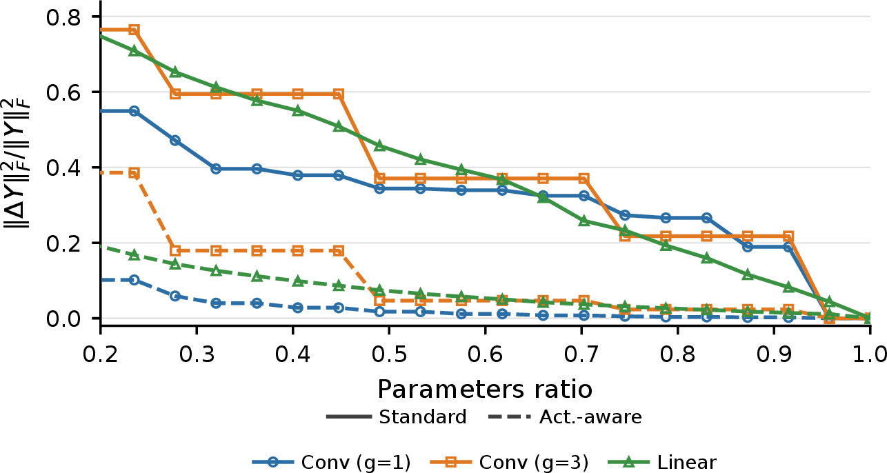
where \(D\) is some penalty function, and \(\widehat{{\boldsymbol{\mathsfit{W}}}}\) is the approximate tensor. We use equality to denote an arbitrary choice from the argmin when it is non-unique. Traditional SVD-based decomposition corresponds to the case where \(D\) is the Frobenius norm of the (reshaped) parameters, i.e., it penalizes distance in parameter space (see 1 ). We use \(\mathcal{T}^{D}_{P}\bigl({\boldsymbol{\mathsfit{W}}}\bigr)\) to also denote batched computation, where each group’s matrix is decomposed individually. As before, we omit \(\overline{P}\) to simplify notation.
4.1 Activation-Aware Low-Rank Projections↩︎
4.1.0.1 Motivation.
A more natural proxy for task performance is the (expected) distortion in each layer’s outputs. In general, though, we have a calibration dataset (which can be the entire training dataset, a subset of it, etc., and is assumed to consist of i.i.d. samples), used to gather layer activations \(({\boldsymbol{\mathsfit{X}}}^{(i)})_{i=1}^B\), which we then use to estimate the distortion. More concretely, the (empirical) average activation distortion for a layer \(f\) is defined as \[\label{eq:actdis95empirical} \begin{align} \ell^{\mathrm{activ}}({\boldsymbol{\mathsfit{W}}}, P) = \frac{1}{B} \sum_{i = 1}^B\|f({\boldsymbol{\mathsfit{X}}}^{(i)}; {\boldsymbol{\mathsfit{W}}}) \!-\! f({\boldsymbol{\mathsfit{X}}}^{(i)}; \mathcal{T}^{}_{P}\bigl({\boldsymbol{\mathsfit{W}}}\bigr))\|^2_F = \frac{1}{B} \|f({\boldsymbol{\mathsfit{X}}}; {\boldsymbol{\mathsfit{W}}}) - f({\boldsymbol{\mathsfit{X}}}; \mathcal{T}^{}_{P}\bigl({\boldsymbol{\mathsfit{W}}}\bigr))\|^2_F. \end{align}\tag{3}\] Note that the last equality holds when forming a “batch” with the list \(({\boldsymbol{\mathsfit{X}}}^{(i)})_{i=1}^B\). In what follows, our analysis is performed in terms of the intermediate activations \({\boldsymbol{\mathsfit{X}}}\) obtained with the calibration dataset, with the expectation that the results carry over to the test dataset. We now aim to find a low-rank projection operator that minimizes 3 .
4.1.0.2 Which projection is best?
In order to answer this question, we first need to define what “best” should mean. Without loss of generality, fix a group \(g\). Clearly, \(\operatorname{rank}\left(\overline{I}({\boldsymbol{\mathsfit{X}}}) \mathcal{T}^{}_{P}\bigl({\boldsymbol{\mathsfit{W}}}\bigr) \right) \leq P\). Moreover, by the EYM theorem, the best rank-\(P\) approximation of the output of \(f\) in terms of the Frobenius norm is \(\mathcal{T}^{\mathrm{SVD}}_{P}\bigl(\overline{I}({\boldsymbol{\mathsfit{X}}}) \overline{P}({\boldsymbol{\mathsfit{W}}})\bigr)\). Hence, a reasonable notion of an ideal scheme is one that factorizes the parameters in a way that is equivalent to factorizing the outputs of the layer; something better is impossible.
Definition 2. We call a scheme \(\mathcal{T}^{}_{P}\bigl(\cdot\bigr)\) optimal if its distortion is equivalent to directly low-rank truncating the outputs of a layer, i.e., an optimal scheme satisfies \[\begin{align} \| \overline{I}({\boldsymbol{\mathsfit{X}}}) \overline{P}({\boldsymbol{\mathsfit{W}}}) - \mathcal{T}^{\mathrm{SVD}}_{P}\bigl(\overline{I}({\boldsymbol{\mathsfit{X}}})\overline{P}({\boldsymbol{\mathsfit{W}}})\bigr)\|_F = \| \overline{I}({\boldsymbol{\mathsfit{X}}}) \overline{P}({\boldsymbol{\mathsfit{W}}}) - \overline{I}({\boldsymbol{\mathsfit{X}}}) \mathcal{T}^{}_{P}\bigl(\overline{P}({\boldsymbol{\mathsfit{W}}})\bigr)\|_F . \end{align}\]
Recall that each group is factorized separately. Note that a scheme is optimal if and only if it satisfies 2 with the distance function set to the output distortion. In particular, SVD-LLM [4] introduced a formulation of activation-aware factorization for linear layers, although their formulation implicitly assumes full-rank activations. In practice, they address rank-deficient cases with a small diagonal shift, which is, in general, not optimal5. A more general version of their low-rank activation-aware projection method within our framework, which satisfies 2 and explicitly allows for rank-deficient activations, can be defined as follows. For any \((\overline{O}, \overline{I}, \overline{P})\)-expressible function \(f\), let \[\mathcal{T}^{\mathrm{AA}}_{P}\bigl({\boldsymbol{\mathsfit{W}}}\bigr)= \overline{P}{}^{-1}\left({\boldsymbol{\mathsfit{M}}}\mathcal{T}^{\mathrm{SVD}}_{P}\bigl({\boldsymbol{\mathsfit{M}}}^+\overline{P}\left({\boldsymbol{\mathsfit{W}}}\right)\bigr)\right),\] where \({\boldsymbol{\mathsfit{M}}}\) is a batch of whitening matrices for \(\overline{I}({\boldsymbol{\mathsfit{X}}})\), one per group, and the pseudoinverse and matrix multiplications are performed independently across groups.
For the layers and their corresponding \((\overline{O}, \overline{I}, \overline{P})\)-tuples mentioned earlier, this corresponds, as discussed in previous examples, to two sequential sub-layers (e.g., two linear or convolutional layers) that yield computational gains with sufficiently low \(P\). More details are given in 6. Additionally, our scheme remains optimal, as claimed in [prop:optimality].
propositionOptimalityProp \(\mathcal{T}^{\mathrm{AA}}_{P}\bigl(\cdot\bigr)\) is optimal in the sense of 2.
Moreover, the activation distortion that follows from using our framework is readily computable from the artifacts obtained during compression, as shown in [prop:general95activation95aware95distortion].
propositionGeneralActivationAwareDistortionPropAssume that \(f({\boldsymbol{\mathsfit{X}}}; {\boldsymbol{\mathsfit{W}}})\) is \((\overline{O}, \overline{I}, \overline{P})\)-expressible. Then, the activation distortion (as defined in 3 ) incurred when low-rank projecting the parameters with \(\mathcal{T}^{\mathrm{AA}}_{P}\bigl(\cdot\bigr)\) is \(\frac{N}{B}\sum_{g=1}^{G}{\sum_{i=P+1}^U\boldsymbol{\sigma}_{g,i}^2}\), where \(\boldsymbol{\sigma}\) denotes the batched singular values of \({\boldsymbol{\mathsfit{M}}}^{+}\overline{P}({\boldsymbol{\mathsfit{W}}})\) and \(U\) is the total number of singular values per group.
Recall that \(B\) is the batch size (number of calibration samples), and \(N\) is the outer dimension (see the discussion below 1). The main result of [4] follows as a corollary.
4.1.0.3 A simple experiment.
We compare the output distortion of our activation-aware projection with that of standard SVD. In particular, we select three layers of different types, truncate them to various rank ratios, and measure the resulting output distortions on 1024 CIFAR-10 test images (using 1024 training images for calibration). As shown in 1, activation-aware factorization yields significantly lower distortion.
4.2 Computing the Whitening Matrices↩︎
We compute the whitening matrices using an eigendecomposition. Suppose we are given a group \(g\). Let \({\boldsymbol{X}}= \overline{I}({\boldsymbol{\mathsfit{X}}})_g \in \Rspace{N, I}\). We can then compute the eigenvectors and eigenvalues of \(\frac{1}{N}{\boldsymbol{X}}^\top{\boldsymbol{X}}\): \({\boldsymbol{V}}\) and \({\boldsymbol{\Lambda}}\), respectively, and set \({\boldsymbol{M}}= {\boldsymbol{V}}{\boldsymbol{\Lambda}}^{+1/2}\) and \({\boldsymbol{M}}^{+} = {\boldsymbol{\Lambda}}^{1/2} {\boldsymbol{V}}^\top\) (we abuse notation and use \(\cdot^{+1/2}\) to denote the square root of the pseudoinverse).
This procedure is applied (in vectorized form) independently for each group. Second moments can be accumulated incrementally over minibatches, so the method is memory-efficient. Additional details are provided in 7.
4.3 Budgeted Rank Allocation↩︎
Apart from offering output distortion guarantees, our framework is interpretable in the sense that we can measure the output distortion without additional steps (see [prop:general95activation95aware95distortion]). Can that be used to efficiently choose the rank to which each layer should be truncated?
4.3.0.1 The rank allocation problem.
We now turn to the question of how to select the ranks to retain in each layer, \(\{P_l\}_{l=1}^L\). The naive option is to choose a uniform percentage of rank per layer [4]. A more reasonable option, used in the past for the traditional SVD scheme, is the energy-based singular value pruning criterion [20], [24]. While more expensive approaches have been explored, such as training-based rank learning [26], [33] or NAS-based search [27], our main goal is to find a scalable and efficient method. We can define the analog of the energy metric in our setting as follows (it reads as the energy retained in layer \(l\) when keeping up to rank \(P_l\)): \[\begin{align} E_l(P_l) = \frac{\sum_{g=1}^G\sum_{i=1}^{P_l} \boldsymbol{\sigma}_{g,i}^2}{\sum_{g=1}^G \sum_{i=1}^{U_l} \boldsymbol{\sigma}_{g,i}^2} = 1 - \frac{\|f_l({\boldsymbol{\mathsfit{X}}}^{l-1}; {\boldsymbol{\mathsfit{W}}}^l) - f_l({\boldsymbol{\mathsfit{X}}}^{l-1}; \mathcal{T}^{\mathrm{AA}}_{P_l}\bigl({\boldsymbol{\mathsfit{W}}}^l\bigr))\|^2_F}{\|f_l({\boldsymbol{\mathsfit{X}}}^{l-1}; {\boldsymbol{\mathsfit{W}}}^l)\|^2_F}, \end{align}\] where \(l\) denotes the layer index, \(U_l\) the total number of singular values (per group), and \(P_l\) the number retained (per group). Energy-based selection then consists of picking the lowest rank such that a certain energy threshold (manually defined by the user) is retained. We propose instead to solve an optimization problem that maximizes the total retained energy globally: \[\begin{gather} \underset{P_1, \dots, P_L}{\max}\; \sum_{l=1}^L E_l(P_l), \quad \text{subject to }\; \sum_{l=1}^L C_l(P_l) \leq C_{\max} \;\text{and} \; P_l \in \{1,\dots,U_l\}, \end{gather}\] where \(C_l(P_l)\) is some measure of layer complexity (in our case, FLOPs or number of parameters) when keeping up to rank \(P_l\) on layer \(l\), \(U_l\) is the total number of singular values for a group on layer \(l\), and \(C_{\max}\) is the global model complexity budget. Our allocator supports FLOPs and the number of parameters as complexity targets. The optimization problem is an instance of the multiple-choice knapsack problem, and it can be formulated as a binary linear program. Unfortunately, it is known to be NP-hard (for a review, see [46]), which motivates the need for an alternative.
4.3.0.2 A Lagrangian relaxation.
We approach this limitation by using a Lagrangian relaxation of the problem to obtain approximate solutions. It has a time complexity of \(O((I+ D + 1)\sum_l U_l)\), where \(I\) stands for “number of iterations” and \(D\) depends on the spectral properties of the network. In practice, using 300 iterations suffices while taking less than 0.2 seconds, even for the larger models with which we experimented. We provide additional details in 8.1. We note that, concurrent with the development of this work, [39] proposed a very similar idea. Although they discuss it in the context of “water filling”, the resulting algorithm is very similar to ours.
4.3.0.3 Advantages.
Our selection approach has several desirable properties: (1) it has virtually zero additional overhead and does not query the model, unlike brute-force search methods, which can take hours (e.g., [27]), and (2) it provides explicit control over a complexity budget. This reduces the need for manual hyperparameter sweeps to achieve a compression target: a single run is enough.
4.4 Putting It All Together: BALF↩︎
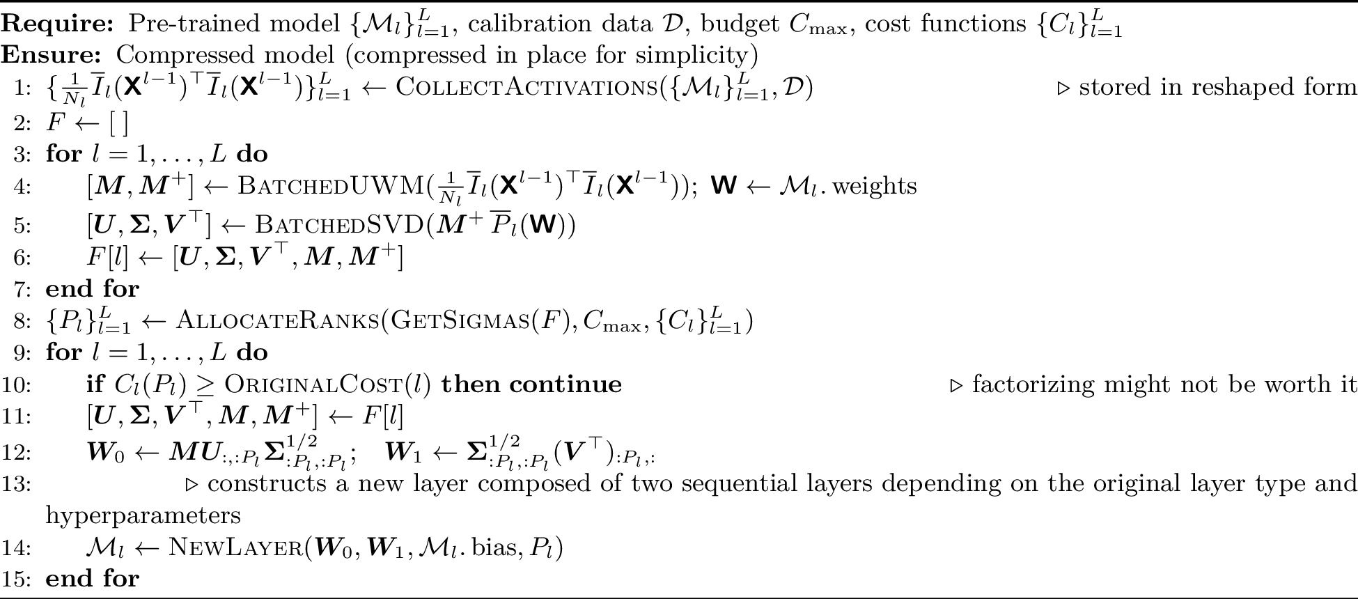
Together, these pieces form BALF. An overview can be found in 2. The routine \(\mathrm{\small NewLayer}\) generates a new layer (consisting of two sequential sub-layers) when given the factorized matrices. In practice, we do not select a manual budget \(C_{\max}\), but rather a ratio (e.g., we might want to obtain a model with 50% of its original FLOPs). Additionally, note that we retain the original layer if compressing it to the selected rank is not computationally advantageous. Similar to SVD-LLM, we precompute activations, whitening matrices, and factors once; they are then cached and can be reused. This is significantly more efficient when generating multiple versions of the same model at different compression ratios (see 12 for more details about the time cost of each step). One alternative is to compute whitening matrices sequentially, using the outputs of already-compressed preceding layers. Another way is to avoid full recomputation but update relevant elements using distorted inputs, similar to a past SVD-LLM version. In preliminary small-scale experiments, we found that recomputing whitening matrices sequentially offered no significant advantage.
4.4.0.1 Handling complex network structures.
Our method operates at the layer level: it modifies each layer’s internal computation without changing inter-layer connections. As a result, it supports complex architectures (e.g., residual connections) without special handling.


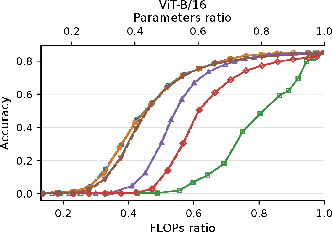
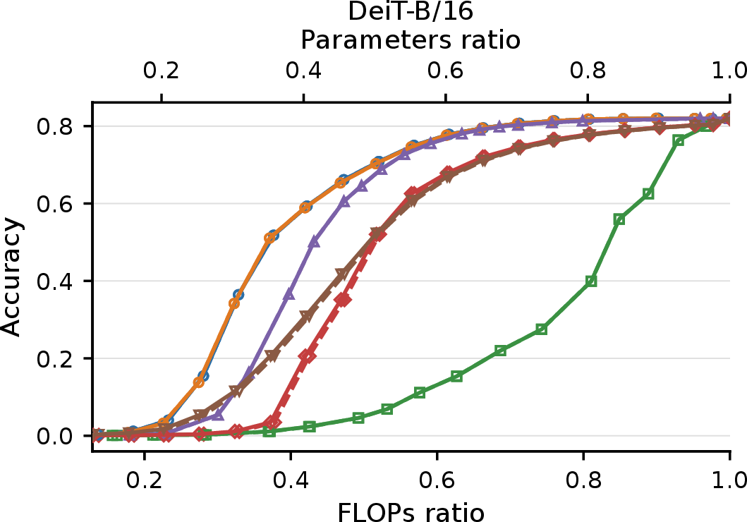

Figure 3: Sweep over compression ratios for different factorization methods across models. Each panel shows parameter–accuracy and FLOP–accuracy curves for each method. BALF-F and BALF-P denote BALF configured with FLOP and parameter-count objectives, respectively. It can be seen that improving the metric targeted by BALF can sometimes incur a nontrivial tradeoff in the non-optimized metric..
4.4.0.2 Bounding the output distortion of a model.
In general, providing bounds on the cumulative model distortion incurred when compressing it is challenging. In [prop:nn95bounds95prop95simple], we show a network-level bound on the output distortion of sequential networks in terms of the individual distortions for each layer \(\ell_l^{\mathrm{activ}}\).
propositionGeneralBoundsPropSimple(Informal) Define a sequential \(L\)-layer network \[\begin{align} {\boldsymbol{\mathsfit{X}}}^{l} = a_l\left(f_{l}({\boldsymbol{\mathsfit{X}}}^{l-1}; {\boldsymbol{\mathsfit{W}}}^{l}) + {\boldsymbol{b}}^l \right) = a_l \left(\overline{O}_{l}\!\big(\overline{I}_{l}({\boldsymbol{\mathsfit{X}}}^{l-1})\overline{P}_{l}({\boldsymbol{\mathsfit{W}}}^{l})\big) + {\boldsymbol{b}}^l\right), \end{align}\] with \({\boldsymbol{\mathsfit{X}}}^{0} = {\boldsymbol{\mathsfit{X}}}\), where \(a_l\) is an element-wise activation function with Lipschitz constant \(A_l\). Moreover, let \(B_l\) be the Lipschitz constant of \(\overline{I}_{l}\) (recall that \(\overline{I}_{l}\) is linear). We assume that all layers are ungrouped. Then, \[\begin{align} &\frac{1}{\sqrt{B}}\bigl\| {\boldsymbol{\mathsfit{X}}}^{L} - \widehat{{\boldsymbol{\mathsfit{X}}}}{}^{L} \bigr\|_F \le \sum_{l=1}^L \Bigl[ A_l\sqrt{\ell^{\mathrm{activ}}_l(P_l)} \prod_{i=l+1}^L\|\overline{P}_i(\widehat{{\boldsymbol{\mathsfit{W}}}}{}^{i})\|_2 A_iB_i \Bigr]. \end{align}\]
A more detailed statement and discussion, along with the proof and special cases, appear in 9. The tightness of the bound depends on the model’s depth and its weights, and it can be loose in deep networks. Even so, it remains conceptually informative.
5 Experiments↩︎
This section presents our experimental results across a range of architectures, datasets, and scales. Our code is available at https://github.com/davidgonmar/BALF. On CIFAR-10 [9], we evaluate ResNet-20 and ResNet-56, while on ImageNet-1K [12], we consider ResNet-18 and ResNet-50 [8], ResNeXt-50 (32\(\times\)4d) and ResNeXt-101 (32\(\times\)8d) with grouped convolutions [10], ViT-B/16 [11], DeiT-B/16 [47], and MobileNetV2 [48]. For all models, every factorizable layer is considered for factorization. Calibration for the main experiments is performed using 1024 images for CIFAR-10 and 8192 images for ImageNet-1K, both uniformly sampled from their respective training datasets. We report accuracy on the CIFAR-10 test set and the ImageNet-1K validation set. The precise settings and hyperparameters are provided in 10.
5.0.0.1 Comparison with factorization baselines.
We first compare BALF against factorization baselines under matched FLOP and parameter count budgets. We conduct a broad sweep over compression ratios to obtain complexity–accuracy curves measured in FLOPs and parameter counts. To assess the contribution of BALF’s components, we compare methods implemented by us: standard SVD and activation-aware SVD, each with both energy-based and uniform rank selection, and BALF, which combines activation-aware decomposition with our rank allocator. For BALF, we consider both FLOP objectives (BALF-F) and parameter-count objectives (BALF-P). For activation-aware methods, which depend on calibration data, we run three calibration seeds and report the mean accuracy. For BALF, whose rank allocation also depends on the calibration data, each reported point averages accuracy and parameter/FLOP counts over the three calibration seeds. In our experiments, the variability induced by the calibration set is negligible, both in terms of compression and accuracy, as can be seen in 4 ¿tbl:tab:results95comparison?.
0.49
@p2cmccc@ Method & \(\Delta\)FLOPs% & \(\Delta\)Params% & \(\Delta\)Top-1 pp
T-ALS & \(-\) & \(-28.57\) & \(-10.90\)
T-ALS & \(-\) & \(-33.33\) & \(-17.60\)
T-ALS-S & \(-\) & \(-28.57\) & \(-3.00\)
T-ALS-S & \(-\) & \(-43.50\) & \(-6.50\)
CP-ALS & \(-\) & \(-51.69\) & \(-3.22\)
CP-ALS & \(-\) & \(-60.47\) & \(-8.03\)
CP-ALS-S & \(-\) & \(-51.69\) & \(-1.91\)
CP-ALS-S & \(-\) & \(-69.23\) & \(-6.70\)
SVD-NAS & \(-58.60\) & \(-68.05\) & \(-13.35\)
ALDS & \(-42.31\) & \(-65.14\) & \(-18.70\)
BALF-F-0.6 & \(-41.18_{\pm 0.00}\) & \(-39.45_{\pm 0.00}\) & \(-15.25_{\pm 0.05}\)
BALF-P-0.6 & \(-13.26_{\pm 0.00}\) & \(-40.01_{\pm 0.00}\) & \(-7.00_{\pm 0.02}\)
BALF-F-0.7 & \(-30.71_{\pm 0.01}\) & \(-28.68_{\pm 0.02}\) & \(-8.50_{\pm 0.01}\)
BALF-P-0.7 & \(-9.13_{\pm 0.01}\) & \(-29.99_{\pm 0.01}\) & \(-3.20_{\pm 0.03}\)
BALF-F-0.8 & \(-20.01_{\pm 0.00}\) & \(-16.74_{\pm 0.00}\) & \(-5.49_{\pm 0.04}\)
BALF-P-0.8 & \(-6.77_{\pm 0.01}\) & \(-22.28_{\pm 0.02}\) & \(-1.69_{\pm 0.02}\)
0.49
@p2cmccc@ Method & \(\Delta\)FLOPs% & \(\Delta\)Params% & \(\Delta\)Top-1 pp
IFM & \(-\) & \(-5.65\) & \(-1.46\)
IFM & \(-\) & \(-20.42\) & \(-10.45\)
ITVSP & \(-\) & \(-4.76\) & \(-3.02\)
ITVSP & \(-\) & \(-9.98\) & \(-10.21\)
DFPC & \(-\) & \(-5.66\) & \(-5.78\)
DFPC & \(-\) & \(-10.92\) & \(-13.88\)
T-ALS & \(-\) & \(-27.54\) & \(-4.49\)
T-ALS & \(-\) & \(-33.33\) & \(-20.14\)
T-ALS-S & \(-\) & \(-27.54\) & \(-2.57\)
T-ALS-S & \(-\) & \(-33.33\) & \(-6.90\)
BALF-F-0.5 & \(-50.03_{\pm 0.02}\) & \(-43.84_{\pm 0.01}\) & \(-13.96_{\pm 0.05}\)
BALF-P-0.5 & \(-28.17_{\pm 0.01}\) & \(-50.06_{\pm 0.01}\) & \(-7.79_{\pm 0.05}\)
BALF-F-0.7 & \(-30.01_{\pm 0.00}\) & \(-21.66_{\pm 0.01}\) & \(-3.50_{\pm 0.01}\)
BALF-P-0.7 & \(-13.60_{\pm 0.00}\) & \(-29.95_{\pm 0.00}\) & \(-1.97_{\pm 0.03}\)
BALF-F-0.8 & \(-20.03_{\pm 0.02}\) & \(-9.73_{\pm 0.01}\) & \(-1.69_{\pm 0.02}\)
BALF-P-0.8 & \(-9.03_{\pm 0.01}\) & \(-21.90_{\pm 0.01}\) & \(-1.11_{\pm 0.01}\)
0.49
@p2cmccc@ Method & \(\Delta\)FLOPs% & \(\Delta\)Params% & \(\Delta\)Top-1 pp
GTP-15.3 & \(-13.07\) & \(0.00\) & \(0.00\)
GTP-8.8 & \(-50.00\) & \(0.00\) & \(-3.50\)
PRACTISE & \(-16.6\) & \(-\) & \(-2.5\)
DC-ViT & \(-16.6\) & \(-\) & \(-0.54\)
BALF-F-0.6 & \(-38.37_{\pm 0.00}\) & \(-39.52_{\pm 0.00}\) & \(-4.10_{\pm 0.03}\)
BALF-P-0.6 & \(-38.71_{\pm 0.00}\) & \(-39.87_{\pm 0.00}\) & \(-4.31_{\pm 0.02}\)
BALF-F-0.7 & \(-28.78_{\pm 0.00}\) & \(-29.64_{\pm 0.00}\) & \(-1.25_{\pm 0.05}\)
BALF-P-0.7 & \(-29.04_{\pm 0.00}\) & \(-29.91_{\pm 0.00}\) & \(-1.34_{\pm 0.02}\)
BALF-F-0.8 & \(-19.22_{\pm 0.00}\) & \(-19.79_{\pm 0.00}\) & \(-0.19_{\pm 0.01}\)
BALF-P-0.8 & \(-19.36_{\pm 0.00}\) & \(-19.94_{\pm 0.00}\) & \(-0.17_{\pm 0.01}\)
0.49
@p2cmccc@ Method & \(\Delta\)FLOPs% & \(\Delta\)Params% & \(\Delta\)Top-1 pp
SVD-NAS & \(-15.09\) & \(-9.00\) & \(-12.54\)
ALDS & \(-2.62\) & \(-37.61\) & \(-16.95\)
LR-S2 & \(-3.81\) & \(-6.24\) & \(-17.46\)
L2+REST & \(-\) & \(-5.00\) & \(-4.42\)
L2+REST & \(-\) & \(-10.00\) & \(-18.47\)
BALF-P-0.7 & \(-2.07_{\pm 0.01}\) & \(-29.72_{\pm 0.02}\) & \(-28.08_{\pm 0.50}\)
BALF-P-0.75 & \(-1.13_{\pm 0.01}\) & \(-24.78_{\pm 0.02}\) & \(-6.17_{\pm 0.05}\)
BALF-P-0.8 & \(-0.23_{\pm 0.00}\) & \(-19.80_{\pm 0.00}\) & \(-0.61_{\pm 0.03}\)
BALF-P-0.9 & \(-0.12_{\pm 0.00}\) & \(-10.69_{\pm 0.05}\) & \(-0.23_{\pm 0.01}\)
BALF-F-0.97 & \(-2.51_{\pm 0.00}\) & \(-1.55_{\pm 0.00}\) & \(-4.89_{\pm 0.02}\)
Figure 4: 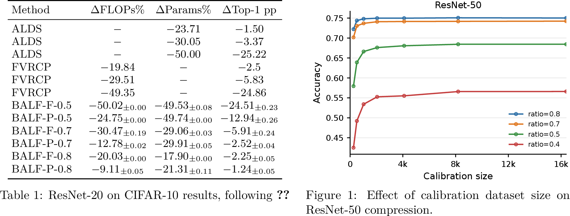 .
.
3 summarizes the complexity–accuracy trade-offs across the different settings. Generally, activation-aware SVD yields consistent gains over plain SVD, with the exact gap varying by configuration. Moreover, our rank allocator enables further low-distortion compression in most cases (but not every case) with respect to the optimized metric (FLOPs or parameter counts). For example, we can reduce the FLOPs of the ResNeXt-101 model by 50% with only about 1.5 percentage points of top-1 accuracy drop. It is important to note, however, that optimizing for one complexity metric can degrade the other. For example, in some cases, setting a parameter-count objective yields substantial gains in parameter count but leads to worse FLOP reduction. For ViTs, the FLOP and parameter-count curves are nearly identical. This is because, ignoring operations outside the linear layers, compressing a linear layer reduces FLOPs by the same amount as it reduces the number of parameters. MobileNetV2 is a notably challenging case for factorization. Activation-aware SVD yields relatively substantial improvements in the parameter-count setting, with the allocator providing a slight additional edge, but FLOP reduction remains difficult.
5.0.0.2 Comparison with other fine-tuning-free compression approaches.
Additionally, we compare BALF with other structured compression approaches in the fine-tuning-free regime. Unless otherwise noted, we take results from their respective papers.
We compare against several pruning and factorization methods, depending on the availability of reported results. These include the pruning methods DFPC [28], IterTVSPrune (ITVSP) [29], IFM [30], FVRCP [49], DC-ViT [31], and PRACTISE [50]; the factorization methods ALDS [24], SVD-NAS [27] and its LR-S2 baseline, and the methods studied in [40]; the token-merging method GTP [51]; and the pruning-restoration method L2+REST [52]. For [40], T-ALS and CP-ALS denote the plain alternating least-squares variants, while the -S variants denote their data-aware counterparts.
We take results from their respective papers, with the following exceptions. DeiT-B/16 results for PRACTISE are those reported by [31], and the no-fine-tuning MobileNetV2 results for ALDS are those reported by [27]. For L2+REST, which reports the number of removed filters, we approximate this quantity as the number of removed parameters. Note that SVD-NAS requires an expensive search procedure on the order of hours. ¿tbl:tab:results95comparison? summarizes the results for ImageNet-1K models, and 4 includes the results for ResNet-20 on CIFAR-10. Overall, BALF achieves performance comparable to most of the methods considered. It outperforms existing methods in some situations, although it is outperformed in others.
5.0.0.3 Compression runtime.
On an RTX 2080 Ti GPU, compressing ImageNet-1K models is completed in minutes: under four minutes for all models we tested. The most expensive steps can be cached, reducing subsequent compression runs to seconds. We provide a comprehensive benchmark and implementation details in 12.
5.0.0.4 Robustness under calibration–evaluation mismatch.
We evaluate the robustness of BALF under distribution shift in the calibration data. We do so by sampling calibration data from shifted datasets: CIFAR-10-C [53] for ResNet-20, and ImageNet-C [53] and ImageNet-V2 [54] for ResNet-18. We then evaluate the compressed models as usual on the original evaluation datasets. We find that results vary depending on the setting. On ImageNet-C and CIFAR-10-C, the effect generally depends on the corruption type and intensity: some corruptions produce only marginal decreases in performance, while more extreme corruptions can substantially affect BALF. In contrast, ImageNet-V2 calibration data yields no degradation, suggesting that BALF is robust to natural calibration shifts.
5.0.0.5 Robustness under calibration dataset size.
We evaluate BALF using different calibration dataset sizes. We find that fewer calibration samples often yield only marginally worse results than those reported in the main experiments (about 256 samples often suffice for CIFAR-10, while about 1024–2048 samples often suffice for ImageNet-1K), depending on the setting. For instance, [fig:calib95size95sweep95resnet5095main] shows a sweep on ResNet-50. Other results, following similar trends, are presented in 11.
5.0.0.6 Limitations and future work.
BALF inherits some limitations from low-rank factorization. For example, depthwise convolutional layers cannot be further compressed within our framework because the only available rank is \(P=1\). More generally, the \((\overline{O},\overline{I},\overline{P})\) framework may not accommodate every layer type. In addition, although BALF reduces theoretical FLOPs and parameter counts, realizing end-to-end speedups can require efficient low-rank operators; for some configurations, taking advantage of the resulting low-rank structure remains challenging in practice (see 11.3).
Our rank allocator is also approximate. In particular, it can undershoot the target budget in specific cases (see 8.1). Although we did not observe this behavior in our experiments, it can occur theoretically for networks with very sharp spectra, for example as a result of low-rank regularization [55]. Extending the allocator to support additional constraint types and concurrent constraints is an interesting direction for future work. Another possible direction is to combine activation-aware projections with more expensive search methods, such as SVD-NAS, which could improve accuracy at the expense of compression time.
Finally, while BALF performs well on the vision models considered in this work, preliminary experiments on LLMs showed degradation relative to reported results from state-of-the-art factorization methods such as SVD-LLM. Since SVD-LLM-like projections are nearly equivalent to ours in practice, this suggests that our rank allocator may not be suitable in all settings.
5.0.0.7 Conclusion.
We introduced BALF, a fine-tuning-free compression pipeline that generalizes activation-aware low-rank factorization beyond linear layers through our \((\overline{O},\overline{I},\overline{P})\)-expressible layer framework. Our theory yields an optimal activation-aware projection even under rank-deficient activations, avoiding ad hoc fixes and providing a closed-form distortion proxy for fast, budgeted rank allocation under explicit FLOP or parameter-count constraints. Empirically, BALF consistently improves the accuracy–complexity trade-off over SVD-based baselines across CNNs and vision transformers, generally achieves competitive performance against other fine-tuning-free compression methods, and runs efficiently, compressing models in minutes on commodity GPUs.
Acknowledgments↩︎
I thank Fernando Sancho Caparrini and Miguel Ángel Martínez del Amor for their valuable comments and suggestions, which helped improve this manuscript. I acknowledge access to computational resources provided by the University of Seville, including an A100 40GB GPU donated through the NVIDIA Hardware Grant, as well as an RTX 4090, and servers managed by the DeepKnowledge group. I am also grateful for the support of the University of Seville through the Programa de Becas de Iniciación a la Investigación (VIIPPIT-2025-II.1).
Appendix Overview↩︎
This appendix is organized as follows:
6 expands on the factorization scheme and provides parameter and FLOP counts for layers before and after low-rank factorization. It includes results for fully connected, ungrouped convolutional, and grouped convolutional layers, and motivates the use of a shared per-group rank for the latter.
7 details the construction of uncentered whitening matrices via eigendecomposition, discusses numerical choices and fallbacks, and describes the incremental estimation of second moments and other details.
8 discusses the specifics of our rank allocator: it specifies the cost model, and presents the previously mentioned Lagrangian relaxation, together with complexity analysis and experimental results on its behavior.
9 states and proves the formal counterpart of [prop:nn95bounds95prop95simple] (discussed in the main text), including simplified forms for special cases.
10 documents the experimental details of our main experiments, including datasets, models, preprocessing, compression protocols, and other important details.
11 includes additional experiments that answer secondary questions, including reports on calibration dataset size ablations, robustness under distribution shift, and practical speedups.
12 describes the end-to-end practical implementation of BALF at a high level and provides timing and peak memory measurements of its different parts.
13 provides a brief analysis of BALF through the lens of [56].
14 collects complete proofs for results deferred from the main text, namely [prop:general95activation95aware95distortion] [prop:optimality] and auxiliary lemmas.
6 Decomposing the Layers and Complexity After Factorization↩︎
In this section, we provide a more thorough discussion of how layers are decomposed. We also provide the parameter counts and FLOP counts before and after decomposition (the latter is used as the cost function in our rank allocator). Given a layer and a rank \(P\), our scheme has the same complexity as basic SVD truncation to rank \(P\); the difference lies in the (expected) quality of the outputs of the factorized layer. We omit biases for simplicity, as these remain constant in the original and factorized layers. \(B\) denotes the batch size. Strictly speaking, the FLOP counts reported below should all be doubled (as it stands, we count each multiply-accumulate as one FLOP), but we omit the doubling factor for readability.
6.1 Fully Connected Layers↩︎
Let the weight be \({\boldsymbol{W}}\in \mathbb{R}^{D_i \times D_o}\). For \({\boldsymbol{X}}\in \Rspace{B, D_i}\), the original layer computes \[f({\boldsymbol{X}}; {\boldsymbol{W}}) = {\boldsymbol{X}}{\boldsymbol{W}}.\]
It has a total of \(D_i D_o\) parameters, and takes \(B D_i D_o\) FLOPs.
6.1.0.1 After decomposition.
Given a rank \(P\), we factor the weights into \({\boldsymbol{W}}_{0} \in \Rspace{D_i, P}\) and \({\boldsymbol{W}}_{1} \in \Rspace{P, D_o}\). The decomposed layer becomes \[f({\boldsymbol{X}}; {\boldsymbol{W}}_{0}, {\boldsymbol{W}}_{1}) = ({\boldsymbol{X}}{\boldsymbol{W}}_{0}) {\boldsymbol{W}}_{1}.\]
The total storage needed is the sum of the storage for each matrix, that is, \(P (D_i + D_o)\), while the number of FLOPs is \(B P (D_i + D_o)\) (the computation order is algebraically irrelevant, but the order is important for efficiency).
6.2 2D Convolutional Layers↩︎
Let the kernel be \({\boldsymbol{\mathsfit{W}}}\in \Rspace{C_o, C_i, H_k, W_k}\) and the (per-item) output spatial size be \(H_o \!\times\! W_o\). For an input \({\boldsymbol{\mathsfit{X}}}\in \Rspace{B, C_i, H_i, W_i}\), the original layer computes \[f({\boldsymbol{\mathsfit{X}}}; {\boldsymbol{\mathsfit{W}}}) = {\boldsymbol{\mathsfit{X}}}* {\boldsymbol{\mathsfit{W}}},\] where \(*\) denotes 2D convolution. The total number of parameters is \(C_o C_i H_k W_k\), and the number of FLOPs is \(B H_o W_o C_o C_i H_k W_k\).
6.2.0.1 After decomposition.
Choose a rank \(P\). We factor the kernel into \[{\boldsymbol{\mathsfit{W}}}_{0} \in \Rspace{P, C_i, H_k, W_k} \quad\text{and}\quad {\boldsymbol{\mathsfit{W}}}_{1} \in \Rspace{C_o, P, 1, 1},\] and the layer computes \[f({\boldsymbol{\mathsfit{X}}}; {\boldsymbol{\mathsfit{W}}}_{0}, {\boldsymbol{\mathsfit{W}}}_{1}) = \big({\boldsymbol{\mathsfit{X}}}* {\boldsymbol{\mathsfit{W}}}_{0}\big) * {\boldsymbol{\mathsfit{W}}}_{1}.\] The total number of parameters is \(P (C_i H_k W_k + C_o)\), and the FLOPs are \(B H_o W_o P (C_i H_k W_k + C_o)\). Note that \(H_o\) and \(W_o\) subsume the additional convolution hyperparameters (padding, strides, dilation, etc.).
“Regular” convolutions are a special case of grouped convolutions, but we included a separate discussion for the convenience of the reader. We will now discuss the general case.
6.3 Grouped 2D Convolutional Layers↩︎
Let \(G\) be the number of groups (assume \(C_i\) and \(C_o\) are divisible by \(G\), as is generally required in modern frameworks). The grouped kernel has shape \[{\boldsymbol{\mathsfit{W}}}\in \Rspace{C_o, C_i / G, H_k, W_k}.\] The original grouped convolution computes \[f({\boldsymbol{\mathsfit{X}}}; {\boldsymbol{\mathsfit{W}}}) = {\boldsymbol{\mathsfit{X}}}\;\mathbin{*_{G}}\; {\boldsymbol{\mathsfit{W}}},\] with a total of \(C_o \frac{C_i}{G} H_k W_k\) parameters, and a total of \(B H_o W_o C_o \frac{C_i}{G} H_k W_k\) FLOPs.
6.3.0.1 After decomposition.
Given the per-group rank \(P\), we decompose the weights into \[{\boldsymbol{\mathsfit{W}}}_{0} \in \Rspace{P G, \, C_i / G, \, H_k, \, W_k} \quad\text{and}\quad {\boldsymbol{\mathsfit{W}}}_{1} \in \Rspace{C_o, \, P, \, 1, 1},\] and the layer computes two grouped convolutions in sequence: \[f({\boldsymbol{\mathsfit{X}}}; {\boldsymbol{\mathsfit{W}}}_{0}, {\boldsymbol{\mathsfit{W}}}_{1}) = \big({\boldsymbol{\mathsfit{X}}}\;\mathbin{*_{G}}\; {\boldsymbol{\mathsfit{W}}}_{0}\big) \;\mathbin{*_{G}}\; {\boldsymbol{\mathsfit{W}}}_{1}.\] The total parameter storage across all groups is \(P (C_i H_k W_k + C_o)\), and the FLOPs are \(B H_o W_o P ( C_i H_k W_k + C_o)\).
The intermediate feature map has \(PG\) channels in total—\(P\) per group—but the parameter and FLOP counts simplify to the expressions above.
6.3.1 On the Sharing of Group Ranks↩︎
As noted in the preceding analysis and in the main text, each group shares the same rank \(P\). This is done for two main reasons.
First, as noted above, the decomposition with the same rank per group results in two sequential (grouped) convolutions. Having different ranks per group would mean that, implementation-wise, we would need \(G\) separate convolutions (or at least some kind of bucketing scheme). In practice, this would be very challenging to perform efficiently.
The second reason is that, even if we managed to achieve an optimal implementation, grouped convolutions are, in essence, \(G\) smaller convolutions run in parallel. It is expected that the largest group would generally be a bottleneck for the others, as the smaller groups would have to wait for them.
7 Uncentered Whitening Matrices↩︎
7.1 Formal Definition and Properties↩︎
We first give the exact definition used throughout the text.
Definition 3. We define an uncentered whitening matrix (UWM) \({\boldsymbol{M}}\in \Rspace{I, I}\) for the data \({\boldsymbol{X}}\in \Rspace{N, I}\) as a matrix such that \({\boldsymbol{M}}^\top {\boldsymbol{X}}^\top {\boldsymbol{X}}{\boldsymbol{M}}= N \overline{{\boldsymbol{I}}}_R\), where \(\overline{{\boldsymbol{I}}}_{R} \in \Rspace{I, I}\) is the identity on the first \(R\) coordinates and zero elsewhere, and \(R\) is the rank of \({\boldsymbol{X}}\). We further restrict the definition by requiring that \(\operatorname{row}({\boldsymbol{X}}) = \operatorname{range}({\boldsymbol{M}})\).
The following two properties hold, with notation as in 3.
Proposition 1. The last \(I - R\) columns of a UWM \({\boldsymbol{M}}\) are zero.
Proof. By our definition, \({\boldsymbol{M}}^\top {\boldsymbol{X}}^\top {\boldsymbol{X}}{\boldsymbol{M}}= N \overline{{\boldsymbol{I}}}_R\), which means that the last \(I - R\) columns of \({\boldsymbol{X}}{\boldsymbol{M}}\) are zero, i.e., the last \(I - R\) columns of \({\boldsymbol{M}}\) lie in \(\operatorname{ker}({\boldsymbol{X}})\). These columns also lie in \(\operatorname{row}({\boldsymbol{X}})\). Since \(\operatorname{ker}({\boldsymbol{X}}) \cap \operatorname{row}({\boldsymbol{X}}) = \{0\}\), these columns must be zero. ◻
Proposition 2. It holds that \({\boldsymbol{X}}= {\boldsymbol{X}}{\boldsymbol{M}}{\boldsymbol{M}}^+\).
Proof. Note that \({\boldsymbol{M}}{\boldsymbol{M}}^+\) is the orthogonal projector onto \(\operatorname{range}({\boldsymbol{M}})\). By definition, \(\operatorname{range}({\boldsymbol{M}}) = \operatorname{row}({\boldsymbol{X}})\). Hence, for any \({\boldsymbol{u}}\in \operatorname{row}({\boldsymbol{X}})\), we have \({\boldsymbol{M}}{\boldsymbol{M}}^+{\boldsymbol{u}}= {\boldsymbol{u}}\). It follows that \({\boldsymbol{M}}{\boldsymbol{M}}^+{\boldsymbol{X}}^\top = {\boldsymbol{X}}^\top\). By transposing and noting that orthogonal projectors are symmetric, \({\boldsymbol{X}}= ({\boldsymbol{M}}{\boldsymbol{M}}^+{\boldsymbol{X}}^\top)^\top = {\boldsymbol{X}}{\boldsymbol{M}}{\boldsymbol{M}}^+\). ◻
7.2 Obtaining UWMs in Practice↩︎
We now provide more details about how the uncentered whitening matrices are obtained. We first begin with a discussion of past work.
The naive option to obtain an uncentered whitening matrix is to use the Cholesky decomposition of the second-moment matrix, as explained in [4]. An issue is that we cannot compute it in the case of singular positive-semidefinite matrices. In their implementation6, they address this issue by adding a diagonal shift. Later, in [5], the authors note this issue and propose the use of an SVD-based whitening matrix, which can be used to support data residing in a subspace, although their analysis does not seem to cover this case (at the time of writing, the SVD-LLM V2 code has not been released). Nevertheless, they report slight end-to-end accuracy gains coming from the SVD-based whitening.
As noted in 4.2, we use an eigendecomposition-based scheme, implemented in practice through the \(\mathsf{eigh}\) routine in PyTorch (a routine that obtains the eigenvalues and eigenvectors of a Hermitian (symmetric in the case of \(\mathbb{R}\)) matrix, and is usually faster than calling the corresponding generic eigendecomposition routine). For notational convenience, we assume the eigenpairs are ordered so that the positive eigenvalues appear first. In implementation, this ordering is unnecessary because the construction and subsequent computations are invariant to a simultaneous permutation of the whitening coordinates.
Recall that, for a single group \(g\), with \({\boldsymbol{X}}= \overline{I}({\boldsymbol{\mathsfit{X}}})_g \in \Rspace{N, I}\), we compute \[[{\boldsymbol{V}}, {\boldsymbol{\Lambda}}] = \mathsf{eigh}(\frac{1}{N} {\boldsymbol{X}}^\top {\boldsymbol{X}}),\] and set \[{\boldsymbol{M}}= {\boldsymbol{V}}{\boldsymbol{\Lambda}}^{+1/2}, \quad {\boldsymbol{M}}^{+} = {\boldsymbol{\Lambda}}^{1/2} {\boldsymbol{V}}^\top,\] where \[{\boldsymbol{V}}{\boldsymbol{\Lambda}}{\boldsymbol{V}}^\top = \frac{1}{N} {\boldsymbol{X}}^\top {\boldsymbol{X}}.\]
It is easy to show that it satisfies our definition. It follows that \[{\boldsymbol{\Lambda}}^ {+1/2} {\boldsymbol{V}}^\top {\boldsymbol{X}}^\top {\boldsymbol{X}}{\boldsymbol{V}}{\boldsymbol{\Lambda}}^ {+1/2} = N {\boldsymbol{\Lambda}}^ {+1/2} {\boldsymbol{V}}^\top {\boldsymbol{V}}{\boldsymbol{\Lambda}}{\boldsymbol{V}}^\top {\boldsymbol{V}}{\boldsymbol{\Lambda}}^ {+1/2} = N \overline{{\boldsymbol{I}}}_R,\] \(R\) being the rank of \({\boldsymbol{X}}\). Moreover, it is easy to see that \(\operatorname{row}({\boldsymbol{X}}) = \operatorname{range}({\boldsymbol{M}})\), as required in our definition (see 7.1). Additionally, the pseudoinverse of \({\boldsymbol{\Lambda}}\) (a diagonal matrix) can be obtained efficiently by inverting each nonzero element of the diagonal, while leaving zeros as is (in practice, we use a small numerical threshold). This avoids additional numerical approximation errors when forming \({\boldsymbol{M}}\). We do not perform any additional steps on the whitening matrices.
7.2.0.1 Practical considerations.
We use the linear algebra functions (with CUDA tensors) provided in the PyTorch library. During early experimentation, we used the MAGMA solver [57], which appeared to be more stable, but it was significantly slower than the default (cuSOLVER [58]), which was ultimately used in our experiments. Sporadically, the \(\mathsf{eigh}\) routine is unable to converge. For that reason, we add a fallback to the SVD-based approach described below. In none of our experiments did the fallback also fail.
7.2.0.2 The alternative.
An SVD-based UWM, as proposed in SVD-LLM V2 [5], can be obtained in a similar way with the SVD of \({\boldsymbol{X}}^\top{\boldsymbol{X}}\). Although it is algebraically equivalent, it tends to be slower than our approach.
7.2.0.3 Accumulating the uncentered moments incrementally.
The naive way of obtaining \(\frac{1}{N} {\boldsymbol{X}}^\top {\boldsymbol{X}}\) in practice is to use a single batch, and then cache activations by passing the batch through the network. However, for some networks with high-dimensional features and/or large batch sizes, the memory requirements might make the process expensive or impossible. A nice property (mentioned in [4], but not discussed extensively) is that we can use data batches to accumulate the second moments. Suppose we have \(M\) batches, then, \[\frac{1}{N} {\boldsymbol{X}}^\top {\boldsymbol{X}} = \frac{1}{N} \begin{bmatrix} {\boldsymbol{X}}_{1,:}^\top & \cdots & {\boldsymbol{X}}_{M,:}^\top \\ \end{bmatrix} \begin{bmatrix} {\boldsymbol{X}}_{1,:} \\ \vdots \\ {\boldsymbol{X}}_{M,:} \end{bmatrix} = \frac{1}{N} \left( {\boldsymbol{X}}_{1,:}^\top {\boldsymbol{X}}_{1,:} + \cdots + {\boldsymbol{X}}_{M,:}^\top {\boldsymbol{X}}_{M,:} \right),\] where \(N\) is the total outer dimension after \(\overline{I}\) reshapes the activations (e.g., for convolutions, \(N = B H_o W_o\)). Here, the indexing denotes the selection of a sub-batch. We use this approach in our implementation.
8 Rank Allocation Details↩︎
This section provides details about the rank allocation strategy discussed in 4.3.
Our objective is to select a list \(\{P_l\}_{l=1}^{L}\) denoting the retained rank in each layer, with the objective of maximizing the global retained energy under some cost constraint. We can model this as a binary linear program in the form of a multiple-choice knapsack problem (for a review, see [46]), with decision variables \(\{x_{l,t}\}_{l,t=1}^{L, U_l}\), where \(x_{l,t} \in \{0, 1\}\) denotes whether, at layer \(l\), \(t\) is selected as the maximum retained rank, and \(U_l\) denotes an upper bound on the rank (in our case, the number of singular values). Furthermore, by establishing a function \(C_l(P_l)\) that returns the computational cost (e.g., in FLOPs or number of parameters) of keeping up to rank \(P_l\) at layer \(l\), we can ensure that the complexity of the solution is constrained to some user-set quantity. The binary program can be expressed as:
\[\begin{align} \max_{\{x_{l,t}\}} \quad & \sum_{l=1}^L \sum_{t=1}^{U_l} E_l(t)\, x_{l,t} \\[0.3em] \text{s.t.}\quad & \sum_{t=1}^{U_l} x_{l,t} = 1, && l=1,\dots,L, \\[-0.2em] & \sum_{l=1}^L \sum_{t=1}^{U_l} C_l(t)\, x_{l,t} \le C_{\max}, \\[-0.2em] & x_{l,t} \in \{0,1\}, && \forall\, l,t. \end{align}\]
8.0.0.1 Are there other options for the objective function?
Recall that we use the total retained energy, which is normalized, as the objective function. Following the insights of [prop:nn95bounds95prop95simple] and [prop:nn95bounds95prop95complete] (although they are not tight for deeper networks), one might speculate that, with appropriate accounting of each layer’s importance, we could achieve better results. During our initial experiments, we also evaluated unnormalized distortion as a metric in place of energy and explored layer-wise weightings based on statistics such as output variance and entropy. None of these alternatives improved performance over the method presented here; instead, they increased complexity and posed additional computational overhead and implementation challenges.
8.0.0.2 Measuring the cost.
Our allocator makes use of a cost function. We refer the reader to 6 for the discussion on the cost of regular and factorized layers, both in terms of FLOPs and in terms of the number of parameters. It is clear that not all \(P_l\) selections result in fewer parameters or FLOPs. Given \(P_l\) and a criterion, we decompose the layer only when we achieve gains in terms of that criterion (e.g., a reduction in FLOPs or parameters); see 2. To reflect this in the cost function, we define it as a piecewise linear function, where the first region is monotonically increasing and represents the region where decomposing the layer results in compression, and the second remains constant, denoting that the action of “keeping rank \(P_l\)” will have the cost of the original layer. Summarizing, we define \[C_l(P_l) = \min \{C_l^{\mathrm{orig}}, C_l^{\mathrm{decomp}}(P_l) \}.\]
We emphasize that this step is important so as to inform the solver that we will not factorize a layer if it is not beneficial.
8.1 A Scalable Lagrangian Relaxation↩︎
The aforementioned program can be solved with publicly available libraries (e.g., PuLP if using Python [59]). The issue is that solving it exactly is known to be NP-hard (see [46]). To overcome this, we employ a Lagrangian relaxation. Pseudocode defining our implementation is given in 5. It accepts a hyperparameter \(I\) denoting the number of iterations to use. For a more general discussion, see [60]. In particular, for a fixed multiplier \(\lambda\), our per-layer update solves the relaxed subproblem in [60]: each layer independently selects the rank maximizing \(E_l(t)-\lambda C_l(t)\). We then search over \(\lambda\) by bisection, using the monotonicity of the induced total cost, and return the feasible allocation obtained at the final multiplier. As usual for such a relaxation-based heuristic, the returned primal allocation need not be globally optimal.
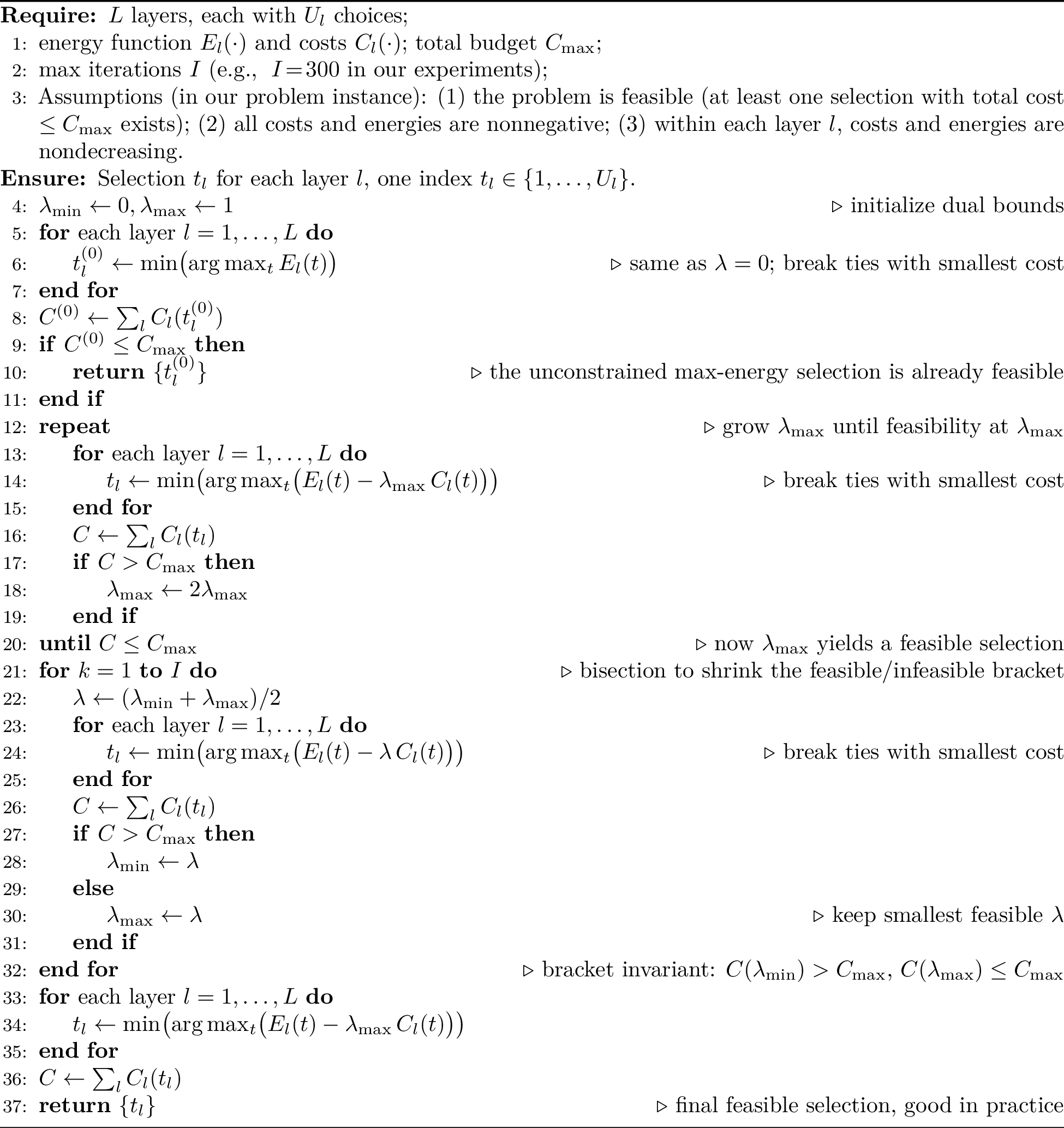
8.1.0.1 Complexity.
Each of the \(I\) outer iterations scans all the candidates once, giving time \(O(I\sum_l U_l)\). The initial doubling to find \(\lambda_{\max}\) adds an additional \(O(D\sum_l U_l)\) factor. Thus, the total time complexity is \(O((I+ D + 1)\sum_l U_l)\) (in the case of a nontrivial solution).
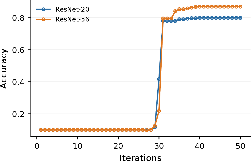
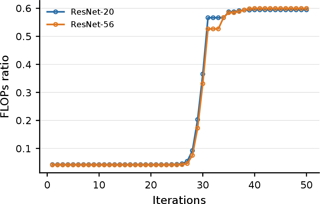
Figure 6: The effect of the number of iterations on CIFAR-10 models. We fix a compression target of 60% of the original FLOPs. The horizontal axis denotes the number of iterations. The vertical axes denote the accuracy achieved (left) and the number of used FLOPs (right). The results stabilize with a relatively small number of iterations..
8.1.0.2 Quality of the solutions.
The algorithm yields an approximate solution, but in every experiment we carried out, it produced good results and saturated (approximately) the target budget. It is, nevertheless, interesting to visualize how the algorithm behaves w.r.t.the number of iterations. 6 compares the number of iterations with two quantities of interest: model accuracy and the actual FLOPs used by the model (when using it with the objective of keeping 60% of the FLOPs).
8.1.0.3 Undershooting.
We describe a specific situation in which our allocator can undershoot the budget. The allocator does not explicitly maximize budget utilization; it maximizes retained energy subject to an upper bound cost constraint. Consequently, the returned solution may use strictly less than the target budget. A simple case occurs when, for each layer, the retained energy curve saturates at some effective rank. Since the algorithm breaks ties in favor of the smallest-cost maximizer, selection will not choose ranks larger than these minimal saturating ranks. If their total cost is already under the budget, the algorithm will not saturate the budget. Although we did not observe this behavior in our experiments, it can theoretically occur for networks with very sharp spectra, for example, as a result of low-rank regularization [55].
8.1.0.4 Implementation details.
We implement the algorithm in Python, as even for larger models, it has a negligible runtime (less than 0.2 seconds in all our experiments, see 12). Moreover, although the energy and cost functions are represented in functional form in the algorithm description, in practice, they are precomputed as vectors for each layer.
9 Bounding the Output Distortion of a Model↩︎
In this section, we provide a more thorough analysis of the claim in [prop:nn95bounds95prop95simple]. We provide a more complete description and its proof. The result applies to sequential (possibly nonlinear) networks with \((\overline{O}, \overline{I}, \overline{P})\)-expressible layers (possibly with biases).
propGeneralBoundsPropComplete Define a sequential \(L\)-layer network \[{\boldsymbol{\mathsfit{X}}}^{0} = {\boldsymbol{\mathsfit{X}}}, \quad {\boldsymbol{\mathsfit{X}}}^{l} = a_l\left(f_{l}({\boldsymbol{\mathsfit{X}}}^{l-1}; {\boldsymbol{\mathsfit{W}}}^{l}) + {\boldsymbol{b}}^l \right) = a_l \left(\overline{O}_{l}(\overline{I}_{l}({\boldsymbol{\mathsfit{X}}}^{l-1})\overline{P}_{l}({\boldsymbol{\mathsfit{W}}}^{l})) + {\boldsymbol{b}}^l \right),\] where \(a_l\) is an element-wise activation function with Lipschitz constant \(A_l\). Moreover, let \(B_l\) be the Lipschitz constant of \(\overline{I}_{l}\) (note that \(\overline{I}_{l}\) is linear and thus Lipschitz-continuous). We restrict our analysis to the case of ungrouped layers. When approximating \({\boldsymbol{\mathsfit{W}}}^{l}\) as a low-rank version, we denote the resulting parameter by \(\widehat{{\boldsymbol{\mathsfit{W}}}}{}^{l}\), and the corresponding cumulatively distorted intermediate activations as \(\widehat{{\boldsymbol{\mathsfit{X}}}}{}^{l}\).
For each layer \(l\), fix the retained rank and let \[\sqrt{\ell^{\mathrm{activ}}_l} = \frac{1}{\sqrt{B}}\bigl\|\;f_{l}({\boldsymbol{\mathsfit{X}}}^{l-1}; {\boldsymbol{\mathsfit{W}}}^{l}) - f_{l}({\boldsymbol{\mathsfit{X}}}^{l-1}; \widehat{{\boldsymbol{\mathsfit{W}}}}{}^{l})\bigr\|_F,\] which reads as the (non-cumulative) error introduced by perturbing \({\boldsymbol{\mathsfit{W}}}^l\to\widehat{\boldsymbol{\mathsfit{W}}}{}^l\). Then, the total output distortion \[d^{(1:L)} =\frac{1}{B}\bigl\|{\boldsymbol{\mathsfit{X}}}^{L} - \widehat{{\boldsymbol{\mathsfit{X}}}}{}^{L}\bigr\|^2_F\] satisfies the bound \[\sqrt{d^{(1:L)}} \;\le\; \sum_{l=1}^L \Bigl[ A_l\sqrt{\ell^{\mathrm{activ}}_l}\;\prod_{i=l+1}^L\|\overline{P}_i(\widehat{{\boldsymbol{\mathsfit{W}}}}{}^{i})\|_2 A_iB_i \Bigr].\]
We follow the convention that the empty product is equal to 1.
Proof. For brevity, we set \({\boldsymbol{W}}^l \equiv \overline{P}_l({\boldsymbol{\mathsfit{W}}}^l)\) (recall that we assume ungrouped layers).
Note that \(\| \overline{O}_l(\cdot) \|_F = \|\cdot \|_F\), as \(\overline{O}_l(\cdot)\) is a composition of permutations and reshapes. It is also true that \(a_l \circ \overline{O}_l = \overline{O}_l \circ a_l\), as \(a_l\) is element-wise.
Then: \[\begin{align} \sqrt{B d^{(1:L)}} &= \| {\boldsymbol{\mathsfit{X}}}^{L} - \widehat{{\boldsymbol{\mathsfit{X}}}}{}^{L} \|_F \\ &= \| a_L(f_{L}({\boldsymbol{\mathsfit{X}}}^{L-1}; {\boldsymbol{\mathsfit{W}}}^{L}) + {\boldsymbol{b}}^L) - a_L(f_{L}(\widehat{{\boldsymbol{\mathsfit{X}}}}{}^{L-1}; \widehat{{\boldsymbol{\mathsfit{W}}}}{}^{L}) + {\boldsymbol{b}}^L) \|_F \\ &= \| a_L(\overline{O}_L(\overline{I}_L({\boldsymbol{\mathsfit{X}}}^{L-1}) {\boldsymbol{W}}^L) + {\boldsymbol{b}}^L) - a_L(\overline{O}_L(\overline{I}_L(\widehat{{\boldsymbol{\mathsfit{X}}}}{}^{L-1}) \widehat{{\boldsymbol{W}}}^L) + {\boldsymbol{b}}^L) \|_F \\ &\leq A_L\|\overline{O}_L(\overline{I}_L({\boldsymbol{\mathsfit{X}}}^{L-1}) {\boldsymbol{W}}^L) + {\boldsymbol{b}}^L - \overline{O}_L(\overline{I}_L(\widehat{{\boldsymbol{\mathsfit{X}}}}{}^{L-1}) \widehat{{\boldsymbol{W}}}^L) - {\boldsymbol{b}}^L \|_F \\ &= A_L\| \overline{I}_L({\boldsymbol{\mathsfit{X}}}^{L-1}) {\boldsymbol{W}}^L - \overline{I}_L(\widehat{{\boldsymbol{\mathsfit{X}}}}{}^{L-1}) \widehat{{\boldsymbol{W}}}^L\|_F \\ &= A_L\| \overline{I}_L({\boldsymbol{\mathsfit{X}}}^{L-1}){\boldsymbol{W}}^L - \overline{I}_L({\boldsymbol{\mathsfit{X}}}^{L-1})\widehat{{\boldsymbol{W}}}^L + \overline{I}_L({\boldsymbol{\mathsfit{X}}}^{L-1}) \widehat{{\boldsymbol{W}}}^L - \overline{I}_L(\widehat{{\boldsymbol{\mathsfit{X}}}}{}^{L-1}) \widehat{{\boldsymbol{W}}}^L \|_F \\ &\leq A_L\| \overline{I}_L({\boldsymbol{\mathsfit{X}}}^{L-1}){\boldsymbol{W}}^L - \overline{I}_L({\boldsymbol{\mathsfit{X}}}^{L-1})\widehat{{\boldsymbol{W}}}^L\|_F + A_L\|\overline{I}_L({\boldsymbol{\mathsfit{X}}}^{L-1}) \widehat{{\boldsymbol{W}}}^L - \overline{I}_L(\widehat{{\boldsymbol{\mathsfit{X}}}}{}^{L-1}) \widehat{{\boldsymbol{W}}}^L \|_F \\ &= A_L\sqrt{B\ell^{\mathrm{activ}}_L} + A_L\|\overline{I}_L({\boldsymbol{\mathsfit{X}}}^{L-1}) \widehat{{\boldsymbol{W}}}^L - \overline{I}_L(\widehat{{\boldsymbol{\mathsfit{X}}}}{}^{L-1}) \widehat{{\boldsymbol{W}}}^L \|_F \\ &\leq A_L\sqrt{B\ell^{\mathrm{activ}}_L} + \| \widehat{{\boldsymbol{W}}}^L \|_2 A_L B_L \| {\boldsymbol{\mathsfit{X}}}^{L-1} - \widehat{{\boldsymbol{\mathsfit{X}}}}{}^{L-1} \|_F \\ &= A_L \sqrt{B\ell^{\mathrm{activ}}_L} + A_L B_L\| \widehat{{\boldsymbol{W}}}^L \|_2 \sqrt{B d^{(1:L - 1)}}. \end{align}\]
By unrolling the recursion and dividing by \(\sqrt{B}\), one arrives at the claimed statement. ◻
9.0.0.1 Some special cases.
There are some interesting instances where the bound reduces to simpler expressions. For example, for fully connected layers, \(B_l = 1\). Moreover, for 1-Lipschitz activations, such as ReLU [61], \(A_l = 1\). For instance, on MLPs with ReLU activations, the bound reduces to \[\begin{align} \sqrt{d^{(1:L)}} \leq \sum_{l = 1}^L \left[ \sqrt{\ell^{\mathrm{activ}}_l} \prod_{i=l+1}^L \| \widehat{{\boldsymbol{W}}}{}^i \|_2 \right]. \end{align}\]
9.0.0.2 Looseness of the bound.
In deep networks, as noted in the main text, this bound is informative rather than practical, as it tends to become looser with depth; the main reason is that the bound involves products of spectral norms. There are some works, for instance [62], that aim to constrain the operator norms of the layers of neural networks. Such constraints would directly tighten our result, but they are not enforced in standard architectures.
10 Experimental Details↩︎
This section provides additional experimental details. All experiments were carried out using the PyTorch library. We make our code public at https://github.com/davidgonmar/BALF. To ensure reproducibility, we include (1) the library code that implements our methods, as well as the baselines, (2) the Python scripts used to carry out the experiments, (3) the Bash scripts used to call the Python scripts with the specific hyperparameters used, and (4) the dependencies and versions used.
10.1 CIFAR-10 Experiments↩︎
10.1.0.1 Models.
Since there are no widely adopted pre-trained CIFAR-10 ResNet model weights, we pre-train the ResNet-20 and ResNet-56 models ourselves, following standard practice. Our CIFAR-10 ResNet implementation is based on the fb.resnet.torch codebase, with the shortcut option set to B: the residual branch uses an identity mapping when the input and output shapes match, and otherwise applies a \(1 \!\times\! 1\) convolution with the appropriate stride followed by batch normalization to match shapes. We use the default PyTorch parameter initialization for all layers.
We use SGD with momentum 0.9, weight decay \(10^{-4}\), and a batch size of 128. The learning rate is initialized to 0.1 and reduced by a factor of 0.1 at epochs 100 and 150. We save the final model checkpoint at epoch 200. For data augmentation, we apply 4-pixel zero-padding followed by a random crop to \(32 \!\times\! 32\) pixels, a random horizontal flip with a probability of 0.5, and per-channel normalization. Under these settings, the final test accuracies are 91.93% for ResNet-20 and 93.18% for ResNet-56.
10.1.0.2 Compression.
In order to obtain the \(k\)-calibration dataset, we pick \(k\) random images uniformly from the training dataset. For all our main experiments, we use 1024 images.
All factorizable layers are considered for compression. For the CIFAR-10 ResNet models, this includes all the convolutional layers, including shortcut layers, and the final fully connected classifier.
10.1.0.3 Dataset processing.
We do not use preprocessing in our calibration dataset and test dataset, other than normalization, so as to mimic inference behavior.
10.2 ImageNet-1K Experiments↩︎
10.2.0.1 Models.
For all the CNNs, we use the implementation provided by the \(\mathsf{torchvision}\) library [63]. We also use their \(\mathsf{V1}\) checkpoints for all the models. For the experiments on vision transformers, we use the implementation and weights provided in the \(\mathsf{timm}\) library [64].
10.2.0.2 Compression.
In order to obtain the \(k\)-calibration dataset, we pick \(k\) random images uniformly from the training dataset. For all our main experiments, we use 8192 images.
All factorizable layers are considered for compression. For the CNNs, this includes all their convolutional layers (including shortcuts) and the linear layers present in the classifier. For the vision transformers, this includes the initial convolutional layer, as well as the linear layers inside attention blocks and MLPs. For the attention blocks, we factorize the merged Q-K-V matrix (implemented in \(\mathsf{timm}\) as a single linear layer).
10.2.0.3 Dataset processing.
Following standard inference practices, we first resize images to \(248\!\times\!248\) for vision transformers (using bicubic interpolation) and to \(256\!\times\!256\) (using bilinear interpolation) for the remaining models, and then center-crop them to \(224\!\times\!224\). We then normalize them following the standard procedure. In particular, we use the default ImageNet-1K mean and standard deviations for all models except for the ViT-B/16, for which we follow the conventions of \(\mathsf{timm}\) and use 0.5 as the mean and standard deviation for all channels. We do this for both the calibration dataset and the validation dataset.
10.3 General Details↩︎
For all our main experiments, we use 300 iterations for our rank allocator (see 8.1). For all the compression sweeps in our experiments section, we conduct a full sweep over the compression targets. For the experiments with our allocator, we select compression ratios (w.r.t.parameter and FLOP counts) between 0.1 and 1.0 in steps of 0.05; additionally, we add 0.975. For the other methods (energy-based methods), we manually select an appropriate set of hyperparameters for each model so that they cover a suitable spectrum of compression ratios.
We follow standard practice when reporting compression results. For FLOP counts, we account for convolutional and fully connected layers, and for ViT models we also count attention FLOPs; we do not count secondary layers such as normalization layers. For FLOP targets, the allocator optimizes only over the FLOPs of layers eligible for factorization. Reported FLOP ratios are then computed after adding back the remaining counted but unoptimized operations. For parameter count results, we include all model parameters in the reported ratios, including parameters of layers that are not compressed. The allocator, however, only optimizes over parameters of layers eligible for factorization.
For some comparison results in the experimental section, we used WebPlotDigitizer7 to extract numeric values from figures when the values were not reported numerically in tables. We took care to perform the extraction as accurately as possible.
10.4 Computational Resources↩︎
Earlier runs of the experiments were executed on a laptop with an RTX 2070 and a node with an RTX 4090. The experiments presented in the final version were each run on a single A100 40GB GPU unless noted otherwise. Preliminary experimentation that did not make it into the paper was conducted on a variety of hardware configurations, including an A100 40GB and other RTX GPUs.
11 Additional Experimental Results↩︎
This section presents some additional experimental results that aim to answer secondary questions.
11.1 How Impactful is the Calibration Dataset Size?↩︎
Although we used 8192 calibration images for ImageNet-1K and 1024 for CIFAR-10, we noticed that moderate calibration dataset sizes worked well. Here, we carry out a sweep over different calibration dataset sizes and compression ratios with parameter compression targets. We use a ResNet-20 and ResNet-56 on CIFAR-10, and ResNet-18, ResNet-50 and ViT-B/16 on ImageNet-1K. 7 shows the different results. As shown, CIFAR-10 is not particularly sensitive to the size of the calibration dataset. On the other hand, the need for larger calibration sets is more apparent on ImageNet-1K. This need increases for larger models (in our case, the ResNet-50), and is exacerbated for higher compression ratios. However, beyond 1024–2048 images, more images yield only marginally better results.
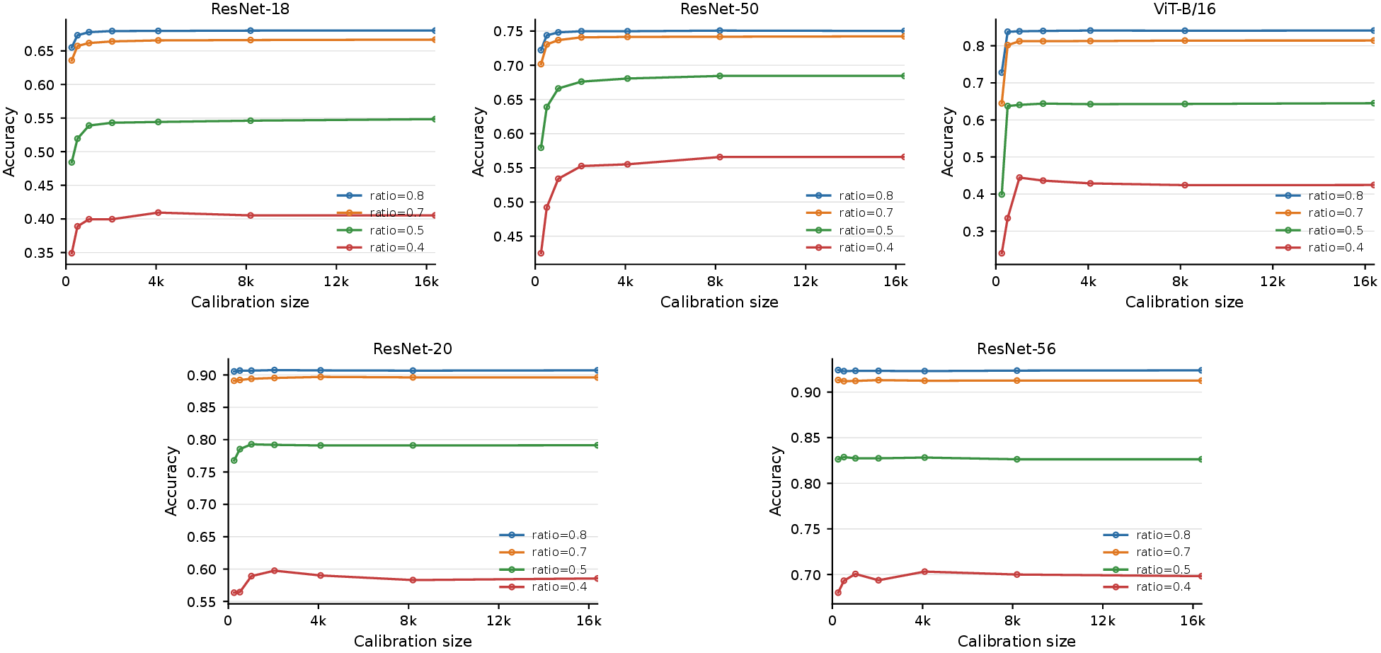
11.2 Robustness under Distribution Shift↩︎
Our method relies on the computation of (uncentered) whitening matrices (over the training dataset in our main experiments) to estimate the optimal low-rank projections. We rely on the i.i.d. assumption to expect transfers to unseen data. As shown over the training–test pairs on CIFAR-10 and ImageNet-1K, we obtain good results. In general, the i.i.d. assumption is common (although seldom discussed) in methods that use calibration data.
Here, we evaluate BALF under calibration–evaluation mismatch. The base models are unchanged and are trained on the original training datasets. We then compute the calibration statistics using shifted data, but evaluate the resulting compressed models on the standard clean evaluation sets. Thus, these experiments test whether BALF remains effective when the calibration data used for compression differs from the data distribution used at evaluation time.
For CIFAR-10, we use ResNet-20 and draw calibration data from CIFAR-10-C [53], while evaluating on the clean CIFAR-10 test set. For ImageNet-1K, we use ResNet-18 and draw calibration data from ImageNet-C [53] or ImageNet-V2 [54], while evaluating on the standard ImageNet-1K validation set. Results for CIFAR-10 appear in 9, results for ImageNet-C appear in 10 11, and results for ImageNet-V2 appear in 12.
For corruption-based datasets, the results vary substantially depending on the corruption type and severity. While some have minor effects on the effectiveness of BALF, others substantially degrade performance. However, performance on the ImageNet-V2 experiment suggests that BALF is robust under natural distribution shifts.
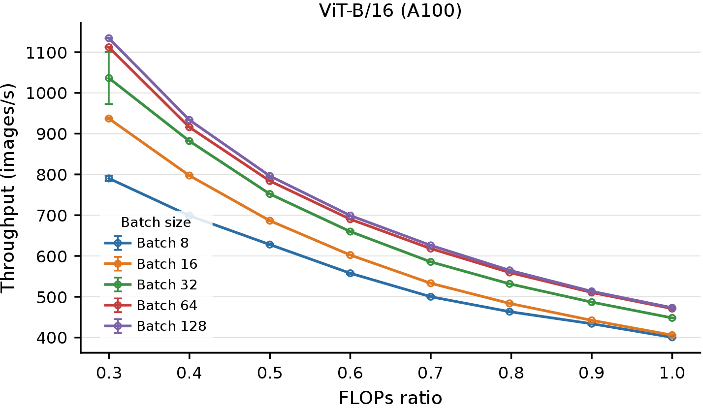
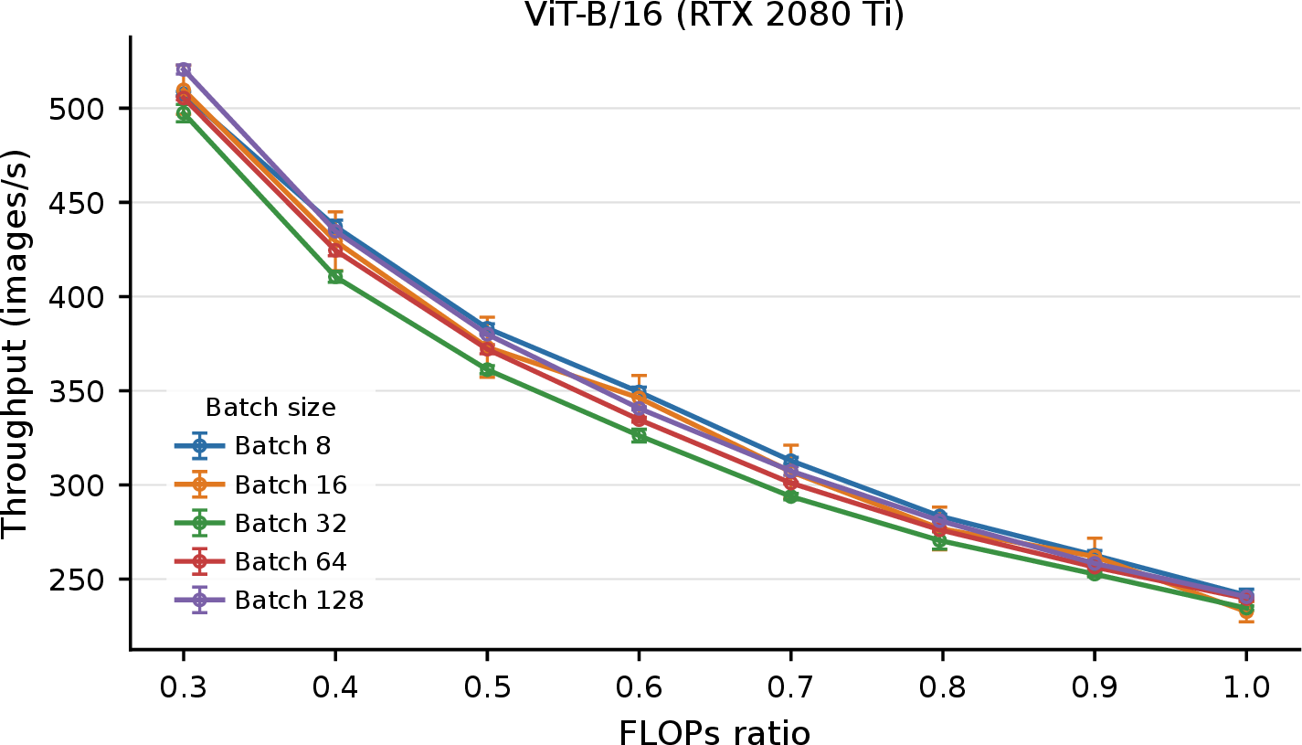
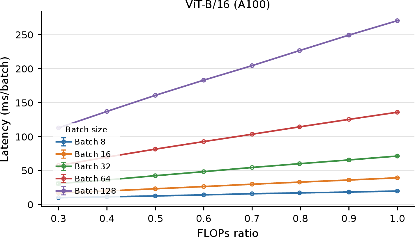
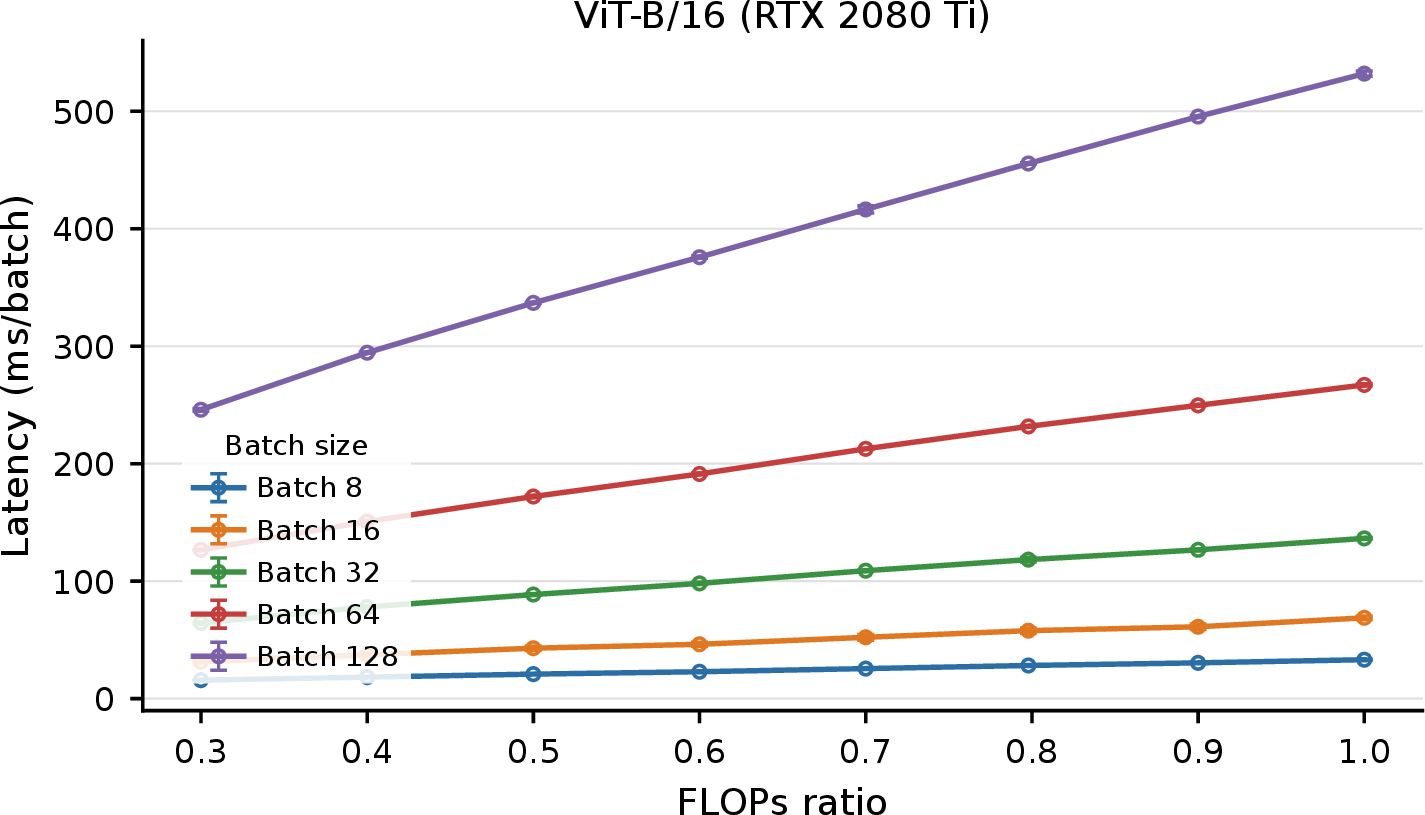


Figure 8: Throughput and latency as a function of FLOP ratio for ViT-B/16 and ResNet-50 on NVIDIA A100 and RTX 2080 Ti GPUs..


Figure 9: Compression–accuracy curves on ResNet-20 when calibration data are drawn from CIFAR-10-C and evaluation is performed on the clean CIFAR-10 test set. Each panel corresponds to one CIFAR-10-C corruption type, with curves shown across target keep ratios and calibration severities..
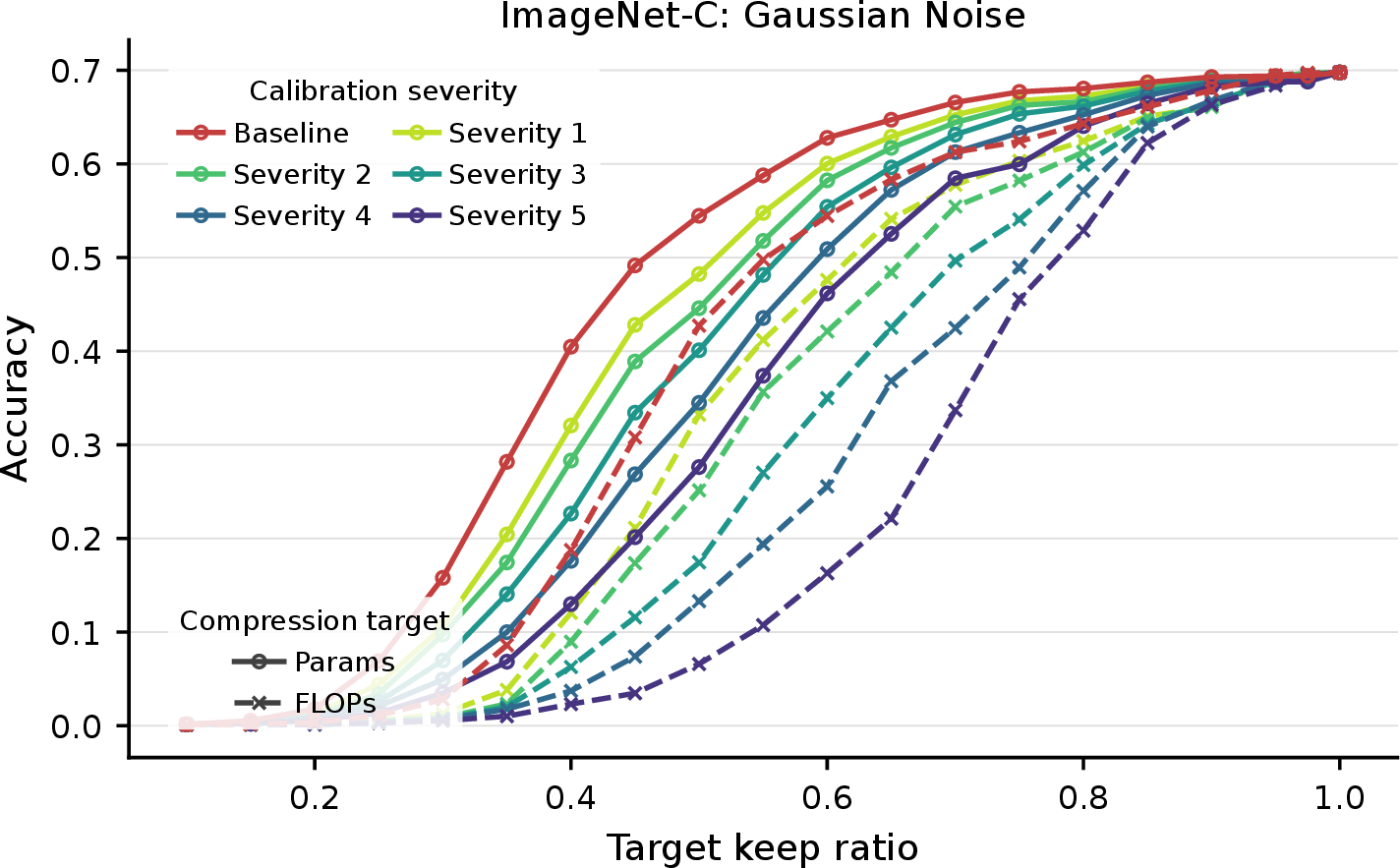
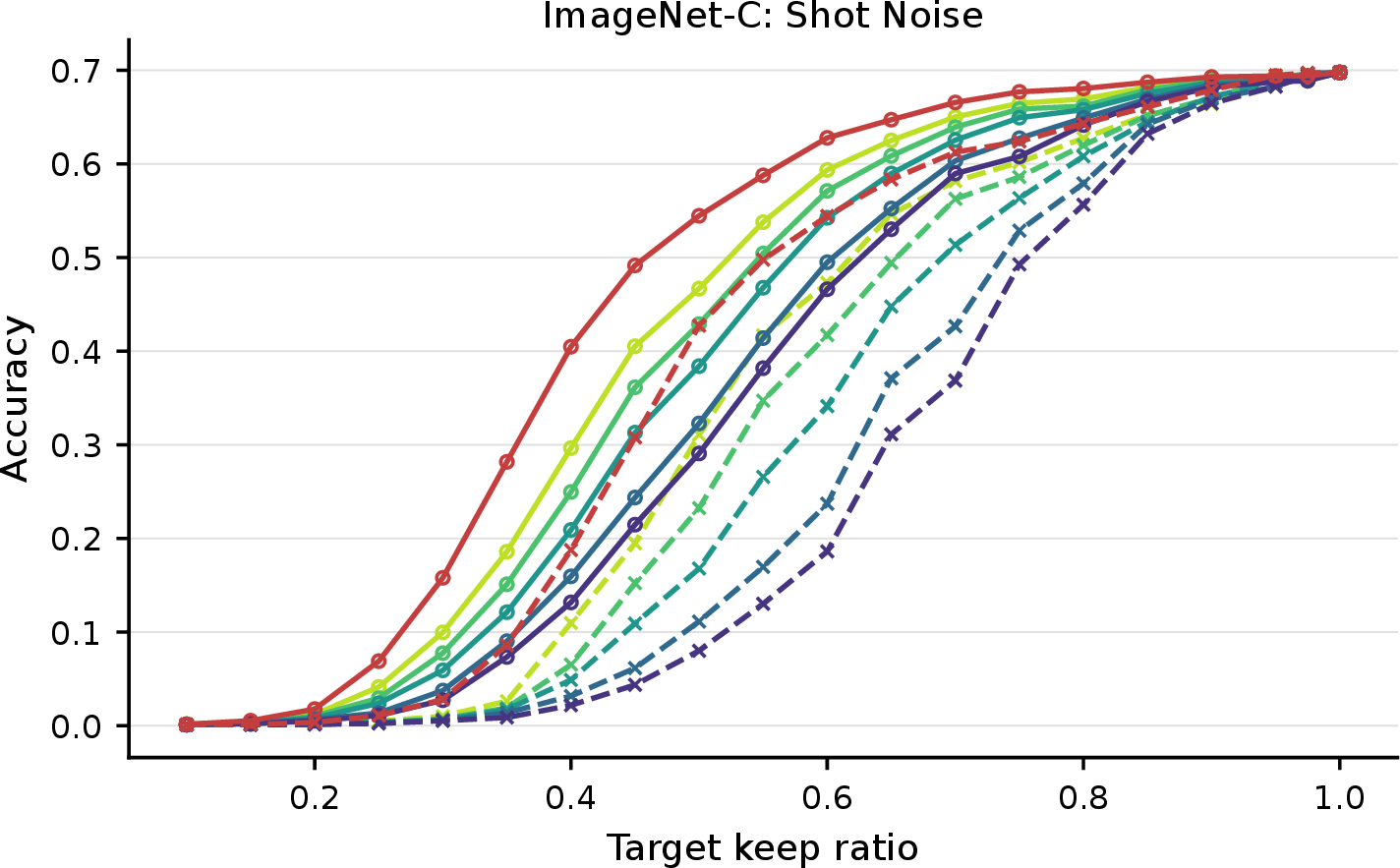
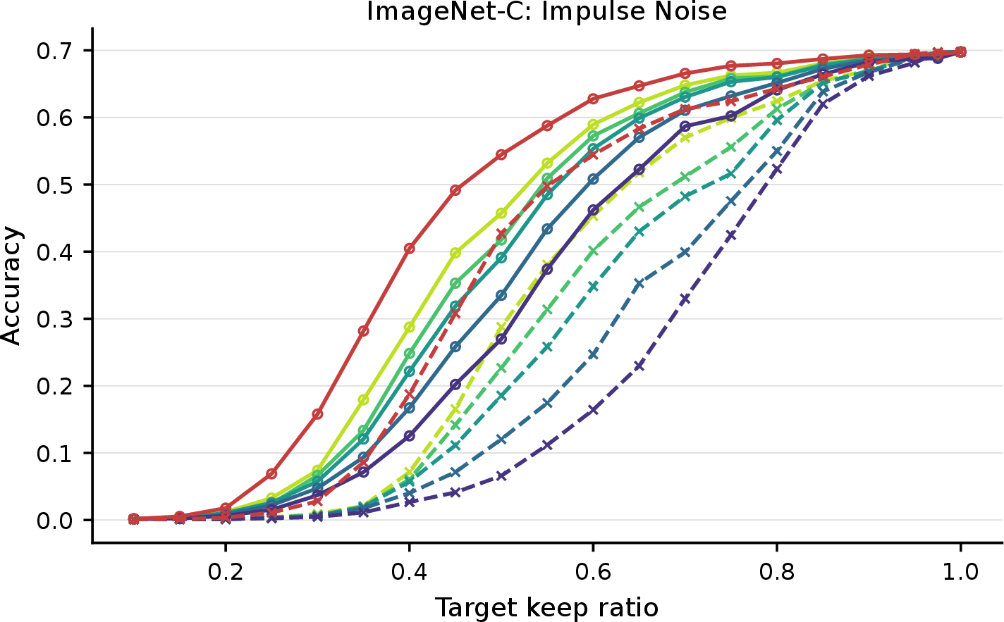
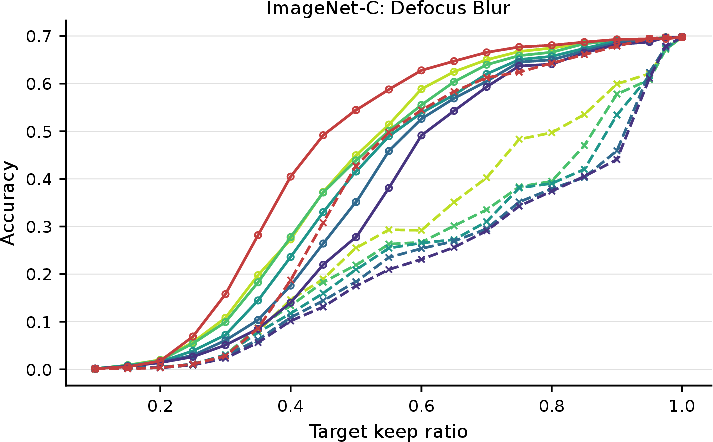
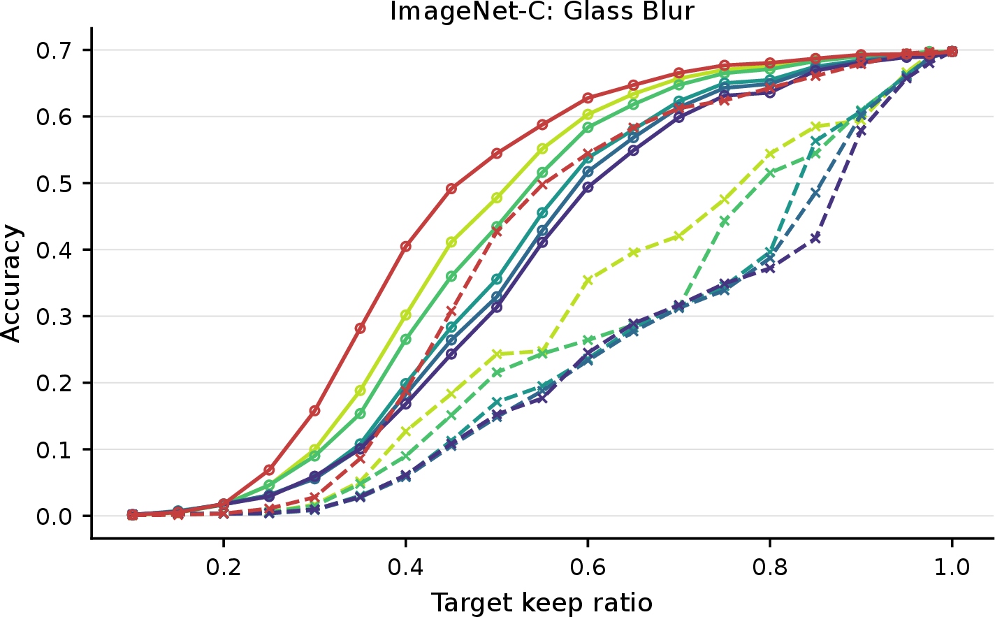
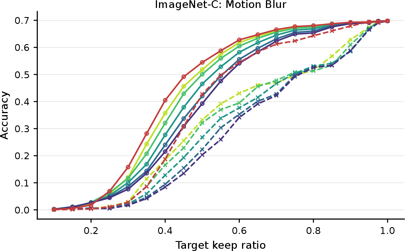
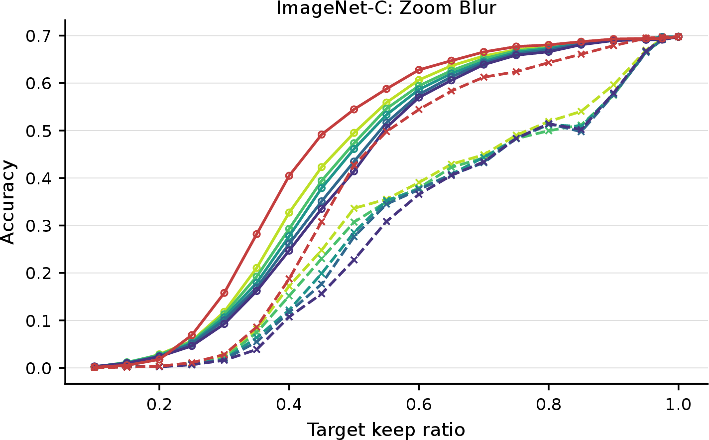
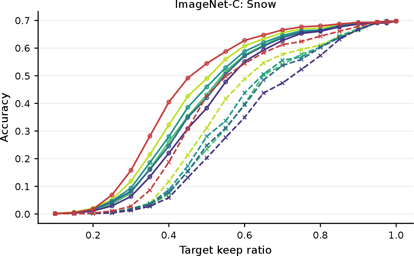
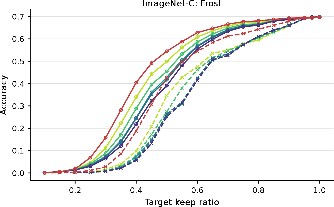
Figure 10: Compression–accuracy curves on ResNet-18 when calibration data are drawn from ImageNet-C and evaluation is performed on the standard ImageNet-1K validation set. Each panel corresponds to one ImageNet-C corruption type from the noise, blur, and selected weather categories..
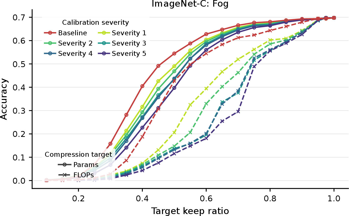
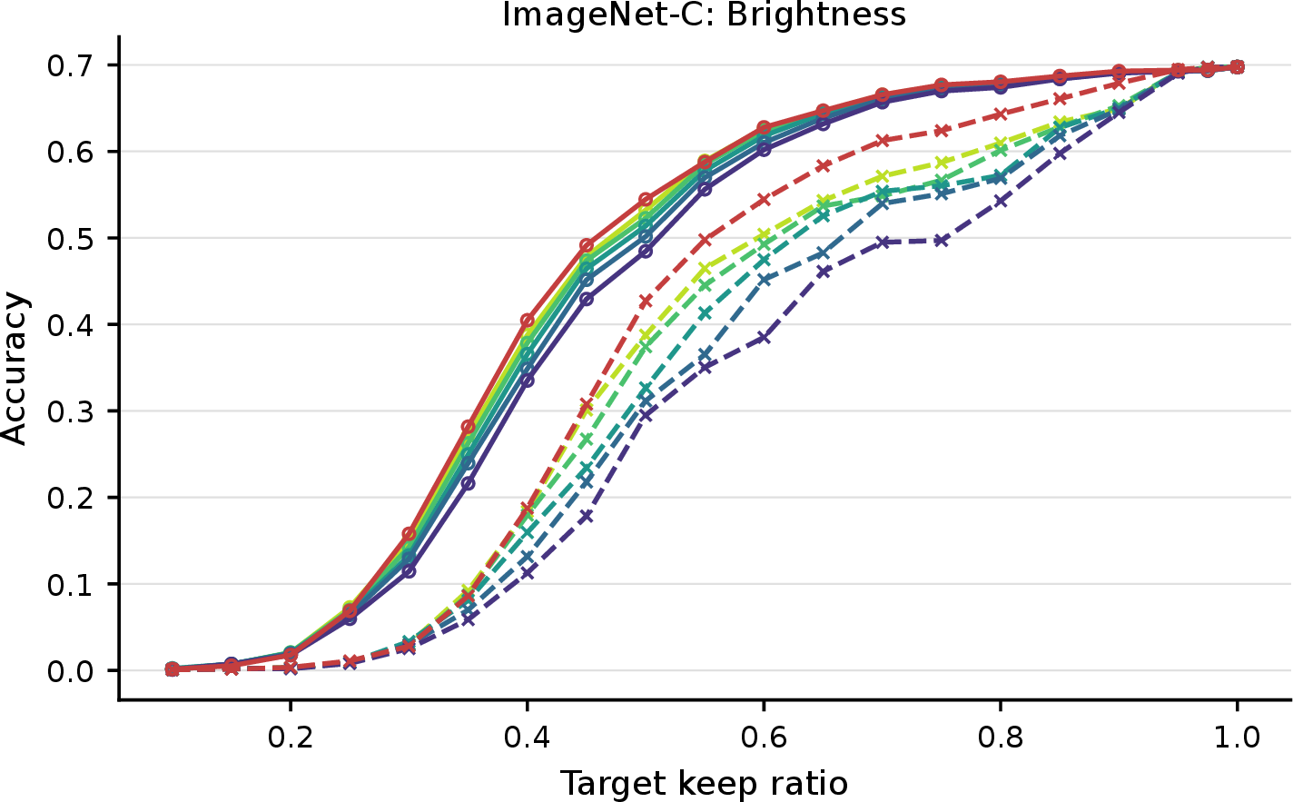

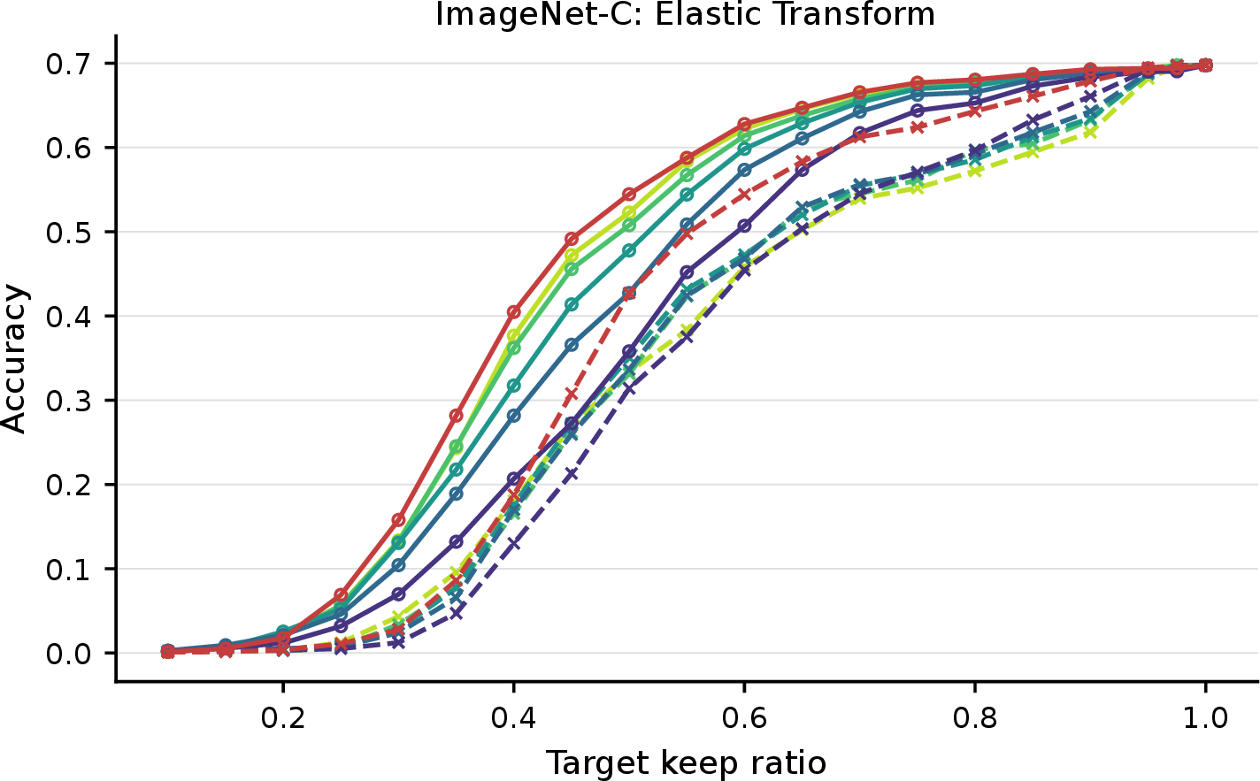
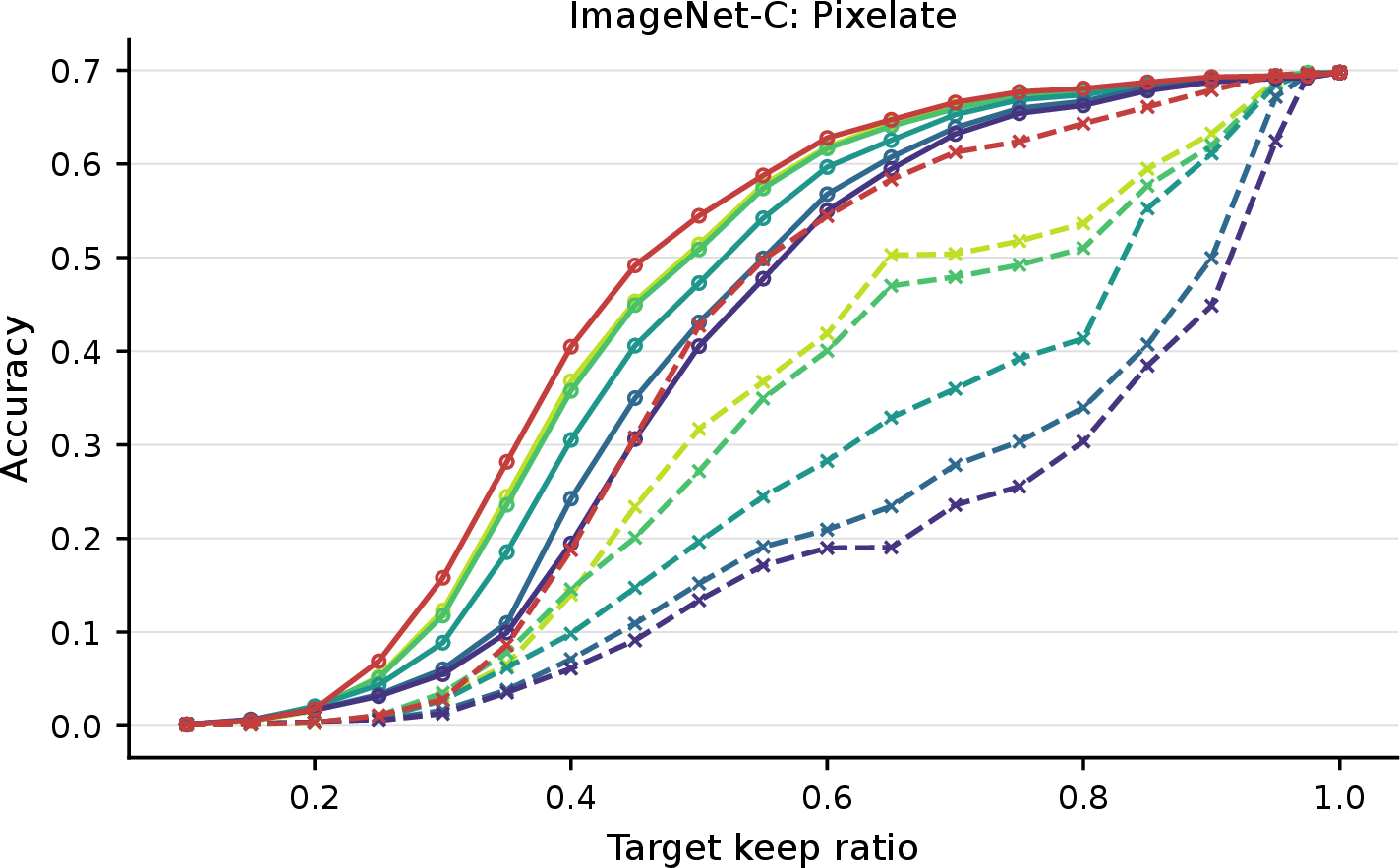
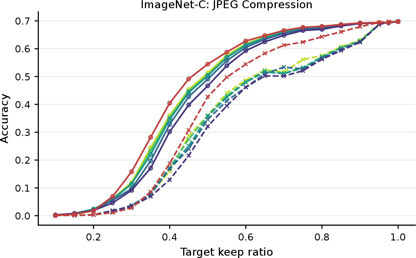
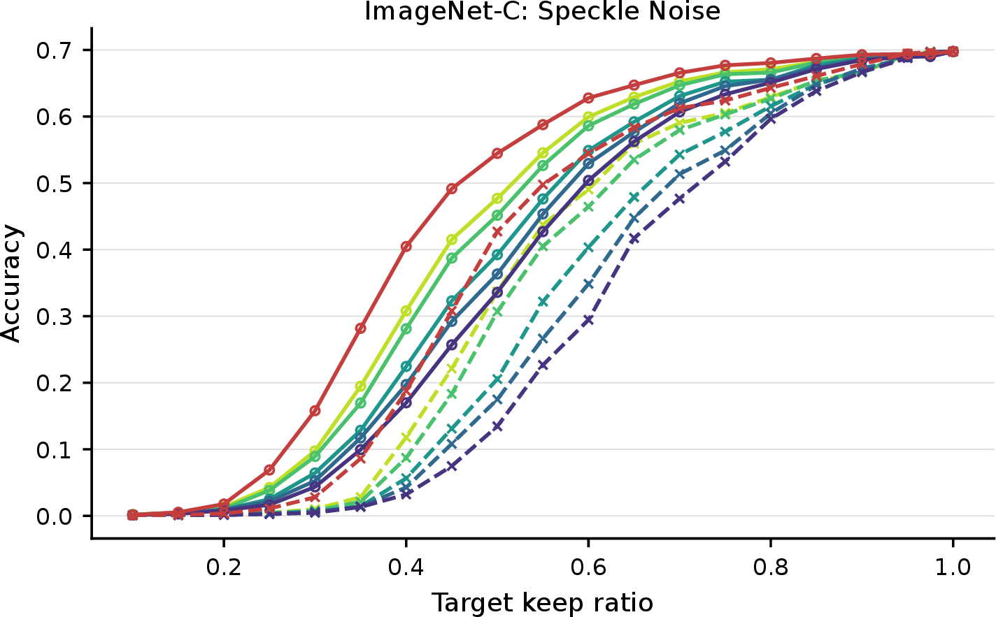
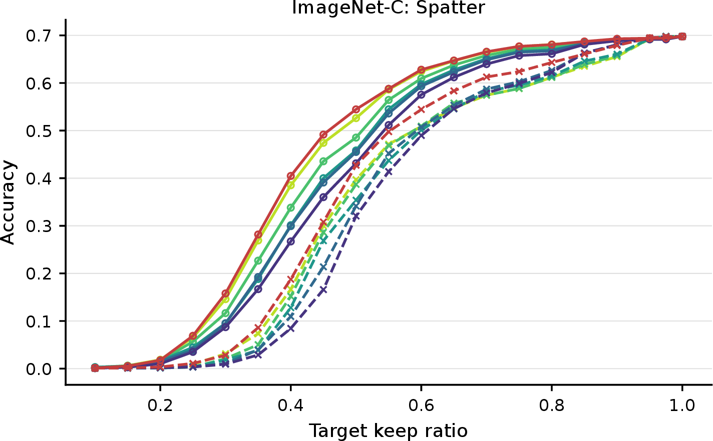
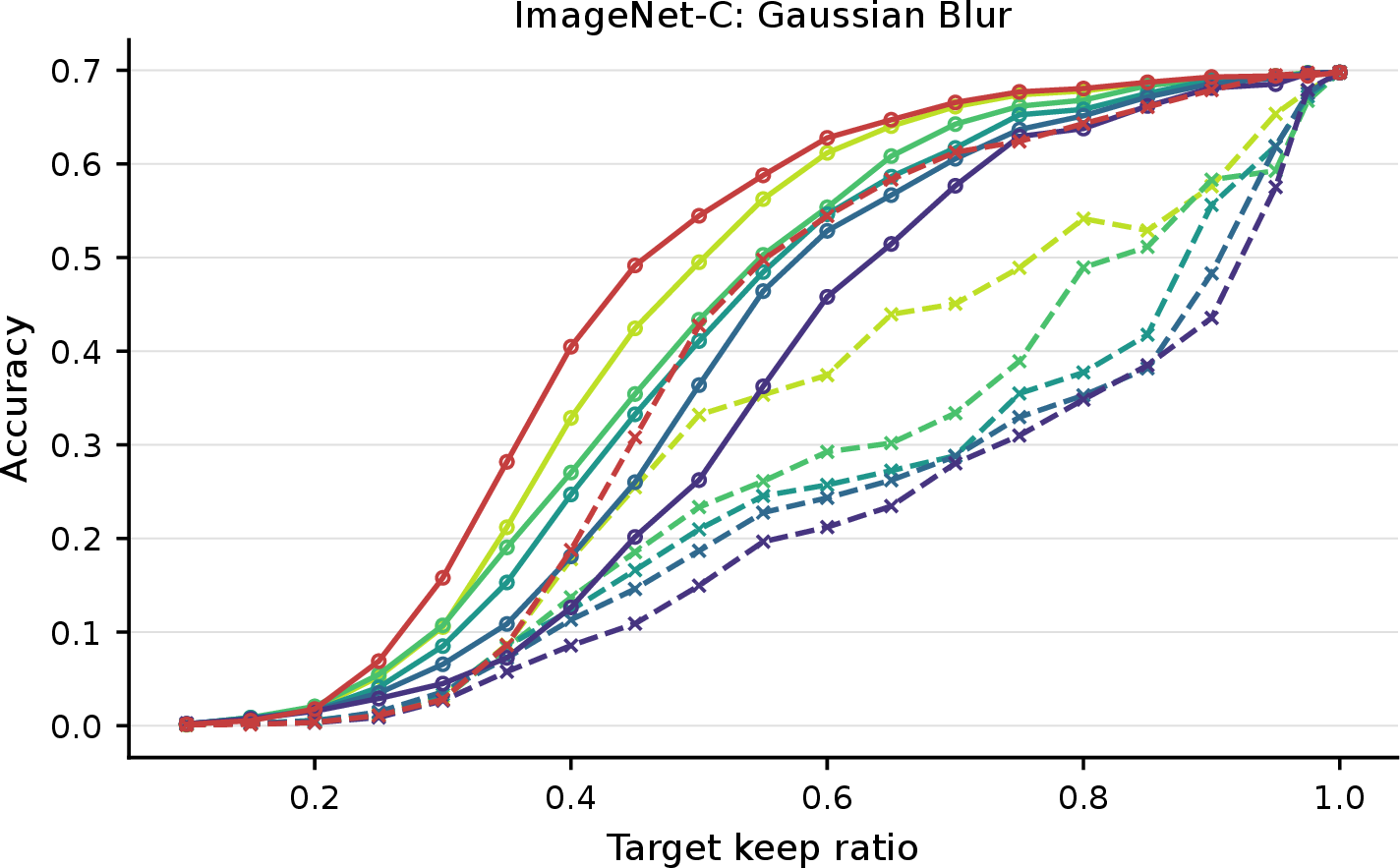
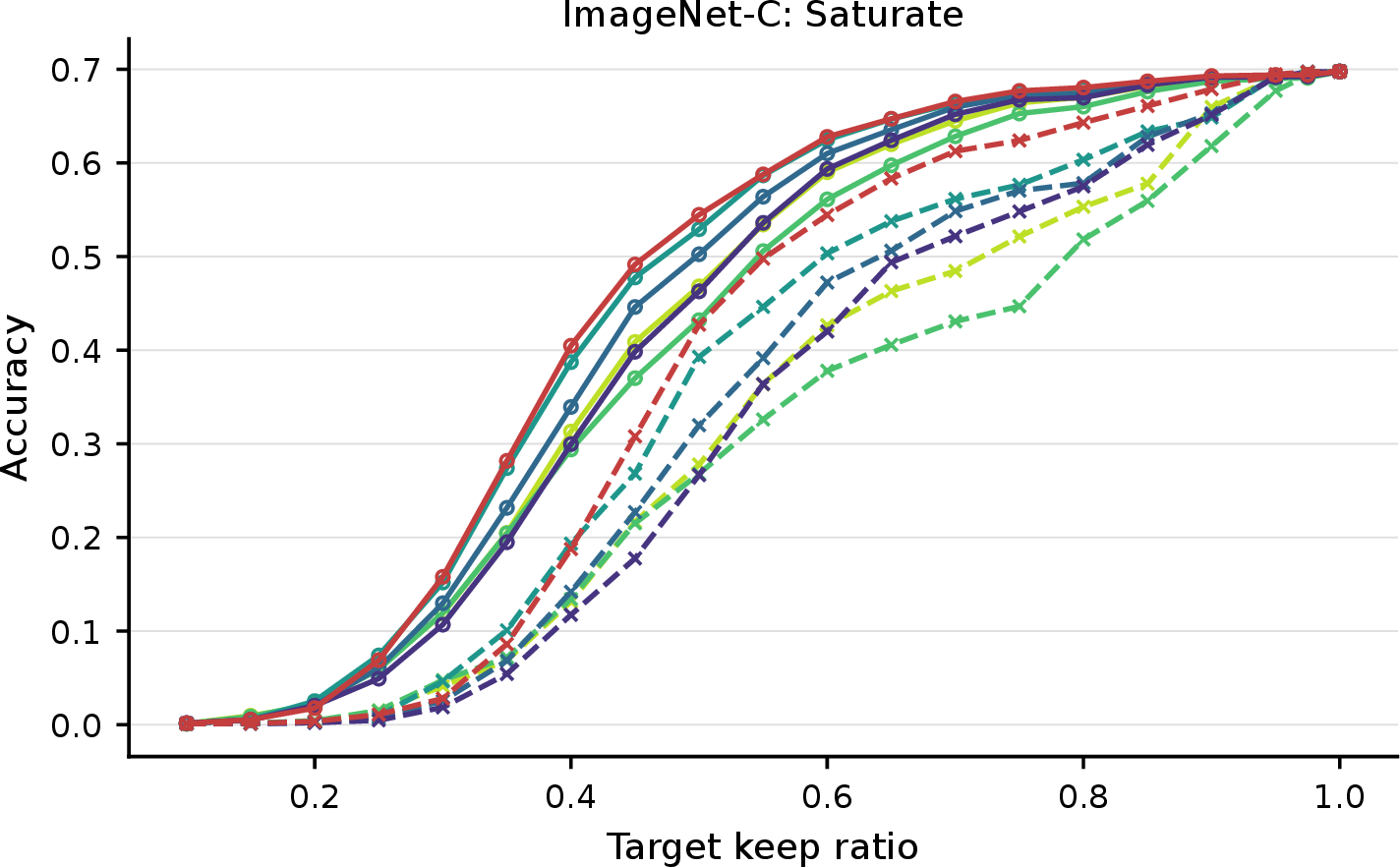
Figure 11: Compression–accuracy curves on ResNet-18 when calibration data are drawn from ImageNet-C and evaluation is performed on the standard ImageNet-1K validation set. Each panel corresponds to one ImageNet-C corruption type from the remaining weather, digital, and extra corruption categories..


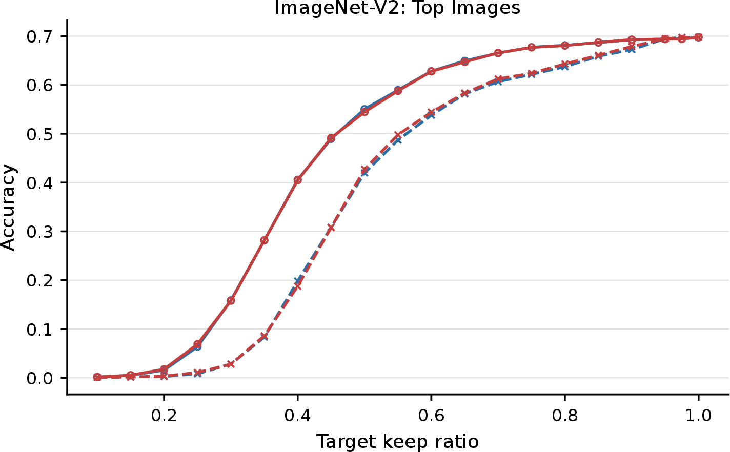
Figure 12: Compression–accuracy curves on ResNet-18 when calibration data are drawn from ImageNet-V2 and evaluation is performed on the standard ImageNet-1K validation set. Each panel corresponds to one ImageNet-V2 variant..
11.3 Speedup of Low-Rank Layers in Practice↩︎
This section discusses the relationship between our compression results (in terms of FLOPs) and the end-to-end speedup obtained in practice. We use basic PyTorch implementations of low-rank operators. In particular, we substitute each original layer with two sequential layers, as described in 6, without any specialized implementation.
We measure the throughput (and latency for completeness) of two ImageNet-1K models (ResNet-50 and ViT-B/16) on an RTX 2080 Ti and an A100 GPU at different compression ratios. Every batch normalization (BN) [65] layer is first removed from the ResNet-50 model so as to mimic the usual inference scenario (where BN layers are folded). We note that our method does not interfere with BN folding in any way.
We found that compression results translate well to actual speedups (see 8) in terms of throughput only in some circumstances. While matrix-multiplication-dominant models such as ViT obtain good speedups, it is important to note that convolutional layers fare worse than linear layers in this regard, and that the theoretical gains are not fully exploited. In particular, on the A100 GPU, no consistent speedup is obtained for ResNet-50.
We expect that specialized operator implementations, including those found in software for edge devices, might be able to fully exploit the compression in terms of speedup. In fact, [66], for instance, were able to obtain near-perfect practical speedups from FLOP reductions on ASICs and FPGAs on ResNet-50 with low-rank layers.
We note that this is, in general, a persistent problem with compression methods (see, e.g., [28], where, without specialized implementations, the actual speedups are significantly lower than the FLOPs reductions). We leave the exploration of more efficient implementations for future work.
12 Runtime and Memory Footprint of BALF↩︎
Our implementation of BALF is conceptually similar to 2, but there are some implementation details that are important to discuss. We first provide a high-level overview of the implementation details:
First, given a calibration dataset, we gather the activation moments. The model runs on the GPU, but the activation moments are offloaded to CPU memory to reduce GPU memory usage and allow compression on lower-end GPUs. Once activation moments are gathered, they can be cached (on disk) for subsequent compression configurations.
Then, whitening matrices and factors are computed on the GPU. These are cached on disk to maintain low memory usage and to avoid recomputation in future runs.
Our rank allocator uses the singular values (computed in the preceding step) to decide how much to compress each layer.
Then, we iterate through the model and substitute the layers with their truncated versions.
| Model | Act. | Fact.+Whit. | Solver | Replace | Misc | Total | Peak Mem. |
|---|---|---|---|---|---|---|---|
| ResNet-18 | \(78.83_{\pm 0.41}\) | \(5.74_{\pm 0.11}\) | \(0.03_{\pm 0.01}\) | \(0.72_{\pm 0.03}\) | \(0.02_{\pm 0.00}\) | \(85.35_{\pm 0.26}\) | \(1.16_{\pm 0.00}\) |
| ResNet-50 | \(97.65_{\pm 0.41}\) | \(5.32_{\pm 0.28}\) | \(0.06_{\pm 0.00}\) | \(0.96_{\pm 0.01}\) | \(0.00_{\pm 0.00}\) | \(103.98_{\pm 0.48}\) | \(1.34_{\pm 0.00}\) |
| MobileNetV2 | \(41.54_{\pm 0.77}\) | \(0.89_{\pm 0.09}\) | \(0.05_{\pm 0.00}\) | \(0.14_{\pm 0.00}\) | \(0.00_{\pm 0.00}\) | \(42.61_{\pm 0.68}\) | \(2.23_{\pm 0.00}\) |
| ResNeXt-50 (32\(\times\)4d) | \(56.97_{\pm 0.93}\) | \(3.91_{\pm 0.06}\) | \(0.06_{\pm 0.01}\) | \(0.41_{\pm 0.01}\) | \(0.00_{\pm 0.00}\) | \(61.35_{\pm 0.98}\) | \(2.29_{\pm 0.00}\) |
| ResNeXt-101 (32\(\times\)8d) | \(181.22_{\pm 1.85}\) | \(19.85_{\pm 0.44}\) | \(0.13_{\pm 0.00}\) | \(1.58_{\pm 0.08}\) | \(0.01_{\pm 0.00}\) | \(202.79_{\pm 1.92}\) | \(4.45_{\pm 0.00}\) |
| ViT-B/16 | \(112.14_{\pm 0.47}\) | \(10.59_{\pm 0.19}\) | \(0.11_{\pm 0.03}\) | \(1.33_{\pm 0.12}\) | \(0.00_{\pm 0.00}\) | \(124.17_{\pm 0.57}\) | \(0.83_{\pm 0.00}\) |
| DeiT-B/16 | \(122.44_{\pm 6.79}\) | \(9.87_{\pm 0.24}\) | \(0.06_{\pm 0.00}\) | \(1.20_{\pm 0.06}\) | \(0.00_{\pm 0.00}\) | \(133.57_{\pm 7.07}\) | \(0.83_{\pm 0.00}\) |
For a thorough examination of the implementation, we refer the reader to our code8. 1 presents the runtime breakdown and peak memory usage of our method on different models on the ImageNet-1K dataset, evaluated on an RTX 2080 Ti GPU. We use 8192 calibration samples (as in our main experiments), divided into batches of 64 samples. All other parameters match those used in the main experiments. We note that the peak memory usage typically occurs during the computation of activation moments, and that using smaller batch sizes can further reduce it.
The only hyperparameters that are expected to affect the runtime of our method are the number of calibration samples and the number of solver iterations. For the first, it is only expected to affect (linearly) the activation-gathering phase (Act. in 1).
Second, the number of solver iterations affects (linearly) the time it takes to produce a solution (Solver in 1). Its runtime is negligible (less than 0.15 seconds in the runs of this section, using 300 iterations).
Finally, we reiterate that the most expensive steps (activation moment gathering and factorization/whitening) are cached, allowing one to obtain different models with different compression configurations in a matter of seconds on average, even on lower-end hardware, after the first run. We also note that our implementation was not particularly optimized (as compression time is not a bottleneck in our evaluations), and that further runtime gains are probably attainable.
13 A Post-Hoc Interpretation via [56]↩︎
Recent work by [56] provides interesting insights into the factorization of neural networks from an information-geometric point of view. BALF has an interesting interpretation through the lens of their framework.
Let \(\widehat{{\boldsymbol{\mathsfit{W}}}}\) denote the low-rank approximation of a parameter tensor. They posit that general activation-aware factorization approaches solve an optimization problem equivalent to minimizing the squared output mismatch under an i.i.d. Gaussian noise model with identity covariance. Translating that to our framework, we obtain \[\begin{align} \arg \min_{\{\widehat{{\boldsymbol{\mathsfit{W}}}}{}^l\} \in \widehat{\mathcal{M}}} &\;\sum_{l=1}^L \left\| \overline{I}_l({\boldsymbol{\mathsfit{X}}}^{l-1}) \overline{P}_l({\boldsymbol{\mathsfit{W}}}^l) - \overline{I}_l({\boldsymbol{\mathsfit{X}}}^{l-1}) \overline{P}_l(\widehat{{\boldsymbol{\mathsfit{W}}}}{}^l) \right\|_F^2 \\ = \arg \min_{\{\widehat{{\boldsymbol{\mathsfit{W}}}}{}^l\} \in \widehat{\mathcal{M}}} &\;\sum_{l=1}^L \sum_{g=1}^{G_l} \left\| \overline{I}_l({\boldsymbol{\mathsfit{X}}}^{l-1})_{g,:,:} \overline{P}_l({\boldsymbol{\mathsfit{W}}}^l)_{g,:,:} - \overline{I}_l({\boldsymbol{\mathsfit{X}}}^{l-1})_{g,:,:} \overline{P}_l(\widehat{{\boldsymbol{\mathsfit{W}}}}{}^l)_{g, :, :} \right\|_F^2 \\ = \arg \min_{\{\widehat{{\boldsymbol{\mathsfit{W}}}}{}^l\} \in \widehat{\mathcal{M}}} &\;\sum_{l=1}^L \sum_{g=1}^{G_l} \sum_{n=1}^{N_l} \left\| \overline{I}_l({\boldsymbol{\mathsfit{X}}}^{l-1})_{g,n,:} \overline{P}_l({\boldsymbol{\mathsfit{W}}}^l)_{g,:,:} - \overline{I}_l({\boldsymbol{\mathsfit{X}}}^{l-1})_{g,n,:} \overline{P}_l(\widehat{{\boldsymbol{\mathsfit{W}}}}{}^l)_{g, :, :} \right\|_2^2 \\ = \arg \min_{\{\widehat{{\boldsymbol{\mathsfit{W}}}}{}^l\} \in \widehat{\mathcal{M}}} &\;D_\mathrm{{KL}}\!\bigl( p_{{\boldsymbol{\mathsfit{W}}}}\,\|\,p_{\smash{\widehat{{\boldsymbol{\mathsfit{W}}}}}\vphantom{{\boldsymbol{\mathsfit{W}}}}} \bigr), \end{align}\] with \[p_{{\boldsymbol{\mathsfit{W}}}}(\cdot) = \prod_{l=1}^L\prod_{g=1}^{G_l} \prod_{n=1}^{N_l} \mathcal{N}\!\left( \cdot \,\middle|\, \overline{I}_l({\boldsymbol{\mathsfit{X}}}^{l-1})_{g,n} \overline{P}_l({\boldsymbol{\mathsfit{W}}}^{l})_g, {\boldsymbol{I}} \right),\] and \[p_{\smash{\widehat{{\boldsymbol{\mathsfit{W}}}}}\vphantom{{\boldsymbol{\mathsfit{W}}}}}(\cdot) = \prod_{l=1}^L\prod_{g=1}^{G_l} \prod_{n=1}^{N_l} \mathcal{N}\!\left( \cdot \,\middle|\, \overline{I}_l({\boldsymbol{\mathsfit{X}}}^{l-1})_{g,n} \overline{P}_l(\widehat{{\boldsymbol{\mathsfit{W}}}}{}^{l})_g, {\boldsymbol{I}} \right).\] In the preceding expressions, the \(n\) index corresponds to the outer dimension (e.g., with \(B H_o W_o = N\) for convolutional layers), \(g\) to the groups, and \(l\) to the layers. The optimization problem generally assumes ranks are fixed (\(\widehat{\mathcal{M}}\) denotes a model with layers truncated to fixed ranks, assumed to be given in advance), and it is only concerned with finding the best low-rank projections.
On the other hand, the problem BALF solves can be formulated as \[\begin{align} \arg \min_{\{\widehat{{\boldsymbol{\mathsfit{W}}}}{}^{l}\} \in \widehat{\mathcal{M}}: C(\widehat{\mathcal{M}}) \leq C_{\max}} &\; \sum_{l=1}^L \frac{ \left\| \overline{I}_l({\boldsymbol{\mathsfit{X}}}^{l-1}) \overline{P}_l({\boldsymbol{\mathsfit{W}}}^{l}) - \overline{I}_l({\boldsymbol{\mathsfit{X}}}^{l-1}) \overline{P}_l(\widehat{{\boldsymbol{\mathsfit{W}}}}{}^{l}) \right\|_{F}^{2} }{ \left\| \overline{I}_l({\boldsymbol{\mathsfit{X}}}^{l-1}) \overline{P}_l({{\boldsymbol{\mathsfit{W}}}}^{l}) \right\|_{F}^{2} } \\ = \arg \min_{\{\widehat{{\boldsymbol{\mathsfit{W}}}}{}^{l}\} \in \widehat{\mathcal{M}}: C(\widehat{\mathcal{M}}) \leq C_{\max}} &\; \sum_{l=1}^L \sum_{g=1}^{G_l} \frac{ \left\| \overline{I}_l({\boldsymbol{\mathsfit{X}}}^{l-1})_{g,:,:} \overline{P}_l({\boldsymbol{\mathsfit{W}}}^{l})_{g,:,:} - \overline{I}_l({\boldsymbol{\mathsfit{X}}}^{l-1})_{g,:,:} \overline{P}_l(\widehat{{\boldsymbol{\mathsfit{W}}}}{}^{l})_{g,:,:} \right\|_{F}^{2} }{ \left\| \overline{I}_l({\boldsymbol{\mathsfit{X}}}^{l-1}) \overline{P}_l({\boldsymbol{\mathsfit{W}}}^{l}) \right\|_{F}^{2} } \\ = \arg \min_{\{\widehat{{\boldsymbol{\mathsfit{W}}}}{}^{l}\} \in \widehat{\mathcal{M}}: C(\widehat{\mathcal{M}}) \leq C_{\max}} &\; \sum_{l=1}^L \sum_{g=1}^{G_l} \sum_{n=1}^{N_l} \frac{ \left\| \overline{I}_l({\boldsymbol{\mathsfit{X}}}^{l-1})_{g,n,:} \overline{P}_l({\boldsymbol{\mathsfit{W}}}^{l})_{g,:,:} - \overline{I}_l({\boldsymbol{\mathsfit{X}}}^{l-1})_{g,n,:} \overline{P}_l(\widehat{{\boldsymbol{\mathsfit{W}}}}{}^{l})_{g,:,:} \right\|_{2}^{2} }{ \left\| \overline{I}_l({\boldsymbol{\mathsfit{X}}}^{l-1}) \overline{P}_l({{\boldsymbol{\mathsfit{W}}}}^{l}) \right\|_{F}^{2} } \\ &= \arg \min_{\{\widehat{{\boldsymbol{\mathsfit{W}}}}{}^l\} \in \widehat{\mathcal{M}}: C(\widehat{\mathcal{M}}) \leq C_{\max}} \;D_\mathrm{{KL}}\!\bigl( p_{{\boldsymbol{\mathsfit{W}}}}\,\|\,p_{\smash{\widehat{{\boldsymbol{\mathsfit{W}}}}}\vphantom{{\boldsymbol{\mathsfit{W}}}}} \bigr), \end{align}\]
with \[p_{{\boldsymbol{\mathsfit{W}}}}(\cdot) = \prod_{l=1}^L\prod_{g=1}^{G_l}\prod_{n=1}^{N_l} \mathcal{N}\!\left( \cdot \,\middle|\, \overline{I}_l({\boldsymbol{\mathsfit{X}}}^{l-1})_{g,n} \overline{P}_l({\boldsymbol{\mathsfit{W}}}^l)_g, \left\| \big(\overline{I}_l({\boldsymbol{\mathsfit{X}}}^{l-1}) \overline{P}_l({\boldsymbol{\mathsfit{W}}}^{l})\big) \right\|_{F}^{2}\,{\boldsymbol{I}} \right),\] and \[p_{\smash{\widehat{{\boldsymbol{\mathsfit{W}}}}}\vphantom{{\boldsymbol{\mathsfit{W}}}}}(\cdot) = \prod_{l=1}^L\prod_{g=1}^{G_l}\prod_{n=1}^{N_l} \mathcal{N}\!\left( \cdot \,\middle|\, \overline{I}_l({\boldsymbol{\mathsfit{X}}}^{l-1})_{g,n} \overline{P}_l(\widehat{{\boldsymbol{\mathsfit{W}}}}{}^{l})_g, \left\| \big(\overline{I}_l({\boldsymbol{\mathsfit{X}}}^{l-1}) \overline{P}_l({\boldsymbol{\mathsfit{W}}}^{l})\big) \right\|_{F}^{2}\,{\boldsymbol{I}} \right).\]
There are two main differences. First, BALF also works under the Gaussian assumption, but with the additional nuance that the variances depend on the per-layer output magnitude (in terms of the squared Frobenius norm). Second, the optimization problem is not only concerned with the low-rank projection scheme given a fixed rank per layer; the selection of ranks under some complexity budget is, itself, baked into the optimization problem. (Note that, strictly speaking, BALF solves the problem approximately in practice.)
We believe this point of view might be an interesting avenue for future research.
14 Deferred Proofs↩︎
In this section, we provide full proofs for the results in the main text that were not covered in other sections of the appendix. Results are restated for the convenience of the reader.
14.1 Proof of [prop:general95activation95aware95distortion]↩︎
Proof. First, observe that \[\label{eq:observation} \|\mathsf{cat}({\boldsymbol{A}}_1,\ldots,{\boldsymbol{A}}_K)\|_F^2 = \sum_{i=1}^K \|{\boldsymbol{A}}_i\|_F^2,\tag{4}\] where \(\mathsf{cat}\) denotes the operation that yields a third-order tensor from a batch of matrices (of the same shape). Therefore, for a batch of distortion matrices, we may analyze each term independently and sum their contributions.
Moreover,
\[\begin{align} \bigl\| f({\boldsymbol{\mathsfit{X}}};{\boldsymbol{\mathsfit{W}}}) - f\bigl({\boldsymbol{\mathsfit{X}}};\mathcal{T}^{\mathrm{AA}}_{P}\bigl({\boldsymbol{\mathsfit{W}}}\bigr)\bigr) \bigr\|_F &= \bigl\| \overline{O}\!\bigl(\overline{I}({\boldsymbol{\mathsfit{X}}})\,\overline{P}({\boldsymbol{\mathsfit{W}}})\bigr) - \overline{O}\!\bigl(\overline{I}({\boldsymbol{\mathsfit{X}}})\,\mathcal{T}^{\mathrm{AA}}_{P}\bigl(\overline{P}({\boldsymbol{\mathsfit{W}}})\bigr)\bigr) \bigr\|_F \\ &= \bigl\| \overline{I}({\boldsymbol{\mathsfit{X}}})\,\overline{P}({\boldsymbol{\mathsfit{W}}}) - \overline{I}({\boldsymbol{\mathsfit{X}}})\,\mathcal{T}^{\mathrm{AA}}_{P}\bigl(\overline{P}({\boldsymbol{\mathsfit{W}}})\bigr) \bigr\|_F, \end{align}\] since \(\overline{O}\) is a composition of reshapes and permutes, which preserve the Frobenius norm.
Fix a group index \(g\) (omitted from the notation below for simplicity). For reference, the dimensions of the different elements are: \(\overline{I}({\boldsymbol{\mathsfit{X}}}) \in \Rspace{N,I}\), \({\boldsymbol{M}}\in \Rspace{I,I}\), \({\boldsymbol{M}}^{+} \in \Rspace{I,I}\), and \(\overline{P}({\boldsymbol{\mathsfit{W}}}) \in \Rspace{I,O}\).
When using activation-aware factorization and truncating to rank \(P\), it follows that \[\begin{align} \ell_{(g)}^{\mathrm{activ}}(P) &= \frac{1}{B} \left\| \overline{I}({\boldsymbol{\mathsfit{X}}})\overline{P}({\boldsymbol{\mathsfit{W}}}) - \overline{I}({\boldsymbol{\mathsfit{X}}}) {\boldsymbol{M}}\mathcal{T}^{\mathrm{SVD}}_{P}\bigl({\boldsymbol{M}}^{+}\overline{P}({\boldsymbol{\mathsfit{W}}})\bigr)\right\|^2_F \notag \\ &\mathrel{\underset{\text{(a)}}{=}} \frac{1}{B}\left\| \overline{I}({\boldsymbol{\mathsfit{X}}}){\boldsymbol{M}}\left( {\boldsymbol{M}}^{+} \overline{P}({\boldsymbol{\mathsfit{W}}}) - \mathcal{T}^{\mathrm{SVD}}_{P}\bigl({\boldsymbol{M}}^{+}\overline{P}({\boldsymbol{\mathsfit{W}}})\bigr) \right) \right\|_F^2 \\ &= \frac{1}{B}\left\| \overline{I}({\boldsymbol{\mathsfit{X}}}){\boldsymbol{M}}{\boldsymbol{U}}\widehat{{\boldsymbol{\Sigma}}} {\boldsymbol{V}}^\top \right\|^2_F \\ &= \frac{1}{B}\operatorname{tr}\left( {\boldsymbol{V}}\widehat{{\boldsymbol{\Sigma}}}^\top {\boldsymbol{U}}^\top {\boldsymbol{M}}^\top \overline{I}({\boldsymbol{\mathsfit{X}}})^\top \overline{I}({\boldsymbol{\mathsfit{X}}}) {\boldsymbol{M}}{\boldsymbol{U}}\widehat{{\boldsymbol{\Sigma}}} {\boldsymbol{V}}^\top\right) \\ &\mathrel{\underset{\text{(b)}}{=}} \frac{N}{B}\operatorname{tr}\left( {\boldsymbol{V}}\widehat{{\boldsymbol{\Sigma}}}^\top \widehat{{\boldsymbol{\Sigma}}} {\boldsymbol{V}}^\top\right) \\ &= \frac{N}{B}\sum_{i=P+1}^U\boldsymbol{\sigma}_i^2, \end{align}\] where the SVD is taken of \({\boldsymbol{M}}^{+}\overline{P}({\boldsymbol{\mathsfit{W}}})\), and \(\widehat{{\boldsymbol{\Sigma}}}\) corresponds to the tail of \({\boldsymbol{\Sigma}}\) after truncating the singular values (i.e., it is equal to \({\boldsymbol{\Sigma}}\) but with the first \(P\) diagonal elements set to 0).
For step (a), note that \(\overline{I}({\boldsymbol{\mathsfit{X}}}) {\boldsymbol{M}}{\boldsymbol{M}}^+ = \overline{I}({\boldsymbol{\mathsfit{X}}})\) (see 7.1).
For step (b), note the following. First, recall from the definition of \({\boldsymbol{M}}\) (see 7.1) that \({\boldsymbol{M}}^\top \overline{I}({\boldsymbol{\mathsfit{X}}})^\top \overline{I}({\boldsymbol{\mathsfit{X}}}) {\boldsymbol{M}}= N\overline{{\boldsymbol{I}}}_R\) (where \(R\) is the rank of \(\overline{I}({\boldsymbol{\mathsfit{X}}})\)); and that \({\boldsymbol{M}}\) has its last \(I - R\) columns set to 0, meaning \({\boldsymbol{M}}^+\) has its last \(I - R\) rows set to 0.
As \({\boldsymbol{U}}\widehat{{\boldsymbol{\Sigma}}}{\boldsymbol{V}}^\top\) corresponds to the SVD tail of \({\boldsymbol{M}}^{+}\overline{P}({\boldsymbol{\mathsfit{W}}}) \in \Rspace{I, O}\), and \({\boldsymbol{M}}^{+}\overline{P}({\boldsymbol{\mathsfit{W}}})\) has its last \(I - R\) rows set to 0, all left singular vectors associated with nonzero singular values lie in the range of \(\overline{{\boldsymbol{I}}}_R\). Hence, \(\overline{{\boldsymbol{I}}}_R{\boldsymbol{U}}\widehat{{\boldsymbol{\Sigma}}}={\boldsymbol{U}}\widehat{{\boldsymbol{\Sigma}}}\), or equivalently \(\widehat{{\boldsymbol{\Sigma}}}^\top{\boldsymbol{U}}^\top\overline{{\boldsymbol{I}}}_R{\boldsymbol{U}}\widehat{{\boldsymbol{\Sigma}}}=\widehat{{\boldsymbol{\Sigma}}}^\top\widehat{{\boldsymbol{\Sigma}}}\). This results in \(\widehat{{\boldsymbol{\Sigma}}}^\top{\boldsymbol{U}}^\top {\boldsymbol{M}}^\top \overline{I}({\boldsymbol{\mathsfit{X}}})^\top \overline{I}({\boldsymbol{\mathsfit{X}}}) {\boldsymbol{M}}{\boldsymbol{U}}\widehat{{\boldsymbol{\Sigma}}} = N\widehat{{\boldsymbol{\Sigma}}}^\top{\boldsymbol{U}}^\top\overline{{\boldsymbol{I}}}_R{\boldsymbol{U}}\widehat{{\boldsymbol{\Sigma}}} = N\widehat{{\boldsymbol{\Sigma}}}^\top\widehat{{\boldsymbol{\Sigma}}}\).
From the observation in 4 , it follows that the total distortion is the sum across each group’s distortion \[\ell^{\mathrm{activ}}(P) = \sum_{g = 1}^G \ell_{(g)}^{\mathrm{activ}}(P) = \frac{N}{B}\sum_{g=1}^{G}{\sum_{i=P+1}^U\boldsymbol{\sigma}_{g,i}^2},\] which completes the proof. ◻
14.2 Proof of [prop:optimality]↩︎
Lemma 1. Let \({\boldsymbol{Y}}\in \Rspace{M, N}\) satisfy \({\boldsymbol{Y}}^\top {\boldsymbol{Y}}= \alpha {\boldsymbol{I}}_N\) with \(\alpha>0\). Then, for any \({\boldsymbol{X}}\in \Rspace{N, K}\), \[\boldsymbol{\sigma}_i({\boldsymbol{Y}}{\boldsymbol{X}}) = \sqrt{\alpha}\boldsymbol{\sigma}_i({\boldsymbol{X}})\] for all \(i\), with singular values padded by zeros if necessary. Consequently, for any \(P \ge 1\), \[\sum_{i=1}^P \boldsymbol{\sigma}_i^2({\boldsymbol{Y}}{\boldsymbol{X}}) = \alpha\sum_{i=1}^P \boldsymbol{\sigma}_i^2({\boldsymbol{X}}).\]
Proof. We have \[({\boldsymbol{Y}}{\boldsymbol{X}})^\top({\boldsymbol{Y}}{\boldsymbol{X}}) = {\boldsymbol{X}}^\top({\boldsymbol{Y}}^\top {\boldsymbol{Y}}){\boldsymbol{X}}= \alpha{\boldsymbol{X}}^\top{\boldsymbol{X}}.\] Hence, the eigenvalues of \(({\boldsymbol{Y}}{\boldsymbol{X}})^\top({\boldsymbol{Y}}{\boldsymbol{X}})\) are exactly \(\alpha\) times those of \({\boldsymbol{X}}^\top{\boldsymbol{X}}\), including zeros. Therefore, \(\boldsymbol{\sigma}_i({\boldsymbol{Y}}{\boldsymbol{X}})=\sqrt{\alpha}\boldsymbol{\sigma}_i({\boldsymbol{X}})\) for all \(i\). Squaring and summing the first \(P\) singular values gives the claim. ◻
Proof. It suffices to prove the result for a single group. Fix a group (its index is omitted from the notation for brevity), and let \({\boldsymbol{W}}= \overline{P}({\boldsymbol{\mathsfit{W}}}) \in \Rspace{I, O}, {\boldsymbol{X}}=\overline{I}({\boldsymbol{\mathsfit{X}}})\in\Rspace{N,I}\), \({\boldsymbol{M}}\in\Rspace{I,I}\), and \({\boldsymbol{M}}^+\in\Rspace{I,I}\) denote the items corresponding to said group, and denote the rank of \({\boldsymbol{X}}\) by \(R\).
We recall the following facts; see 7.1. First, \({\boldsymbol{M}}\) has its last \(I-R\) columns set to \(0\), which forces \({\boldsymbol{M}}^+\) to have its last \(I-R\) rows set to \(0\). Hence, \({\boldsymbol{M}}{\boldsymbol{M}}^+ = {\boldsymbol{M}}{\boldsymbol{I}}_{:,:R}{\boldsymbol{I}}_{:R,:}{\boldsymbol{M}}^+\). Moreover, from the definition of \({\boldsymbol{M}}\), we have \({\boldsymbol{M}}^\top {\boldsymbol{X}}^\top {\boldsymbol{X}}{\boldsymbol{M}}= N \overline{{\boldsymbol{I}}}_R\), and therefore, it holds that \({\boldsymbol{I}}_{:R,:}{\boldsymbol{M}}^\top {\boldsymbol{X}}^\top {\boldsymbol{X}}{\boldsymbol{M}}{\boldsymbol{I}}_{:,:R} = N {\boldsymbol{I}}_R\). It is also true that \({\boldsymbol{X}}{\boldsymbol{M}}{\boldsymbol{M}}^+ = {\boldsymbol{X}}\).
It follows that \[\sum_{i=1}^P \boldsymbol{\sigma}^2_i({\boldsymbol{X}}{\boldsymbol{W}}) = \sum_{i=1}^P \boldsymbol{\sigma}^2_i({\boldsymbol{X}}{\boldsymbol{M}}{\boldsymbol{M}}^+ {\boldsymbol{W}}) = \sum_{i=1}^P \boldsymbol{\sigma}^2_i({\boldsymbol{X}}{\boldsymbol{M}}{\boldsymbol{I}}_{:,:R}{\boldsymbol{I}}_{:R,:}{\boldsymbol{M}}^+ {\boldsymbol{W}}) = N \sum_{i=1}^P \boldsymbol{\sigma}^2_i({\boldsymbol{M}}^+ {\boldsymbol{W}}),\] where the last equality follows from 1.
Hence, \[\begin{align} \|\overline{I}({\boldsymbol{\mathsfit{X}}})\overline{P}({\boldsymbol{\mathsfit{W}}})-\mathcal{T}^{\mathrm{SVD}}_{P}\bigl(\overline{I}({\boldsymbol{\mathsfit{X}}})\overline{P}({\boldsymbol{\mathsfit{W}}})\bigr)\|^2_F &= \sum_{i=P+1}^U \boldsymbol{\sigma}_i^2({\boldsymbol{X}}{\boldsymbol{W}}) \\ &= N \sum_{i=P+1}^U \boldsymbol{\sigma}_i^2({\boldsymbol{M}}^+ {\boldsymbol{W}}) \\ &= \|\overline{I}({\boldsymbol{\mathsfit{X}}})\overline{P}({\boldsymbol{\mathsfit{W}}})-\overline{I}({\boldsymbol{\mathsfit{X}}})\mathcal{T}^{\mathrm{AA}}_{P}\bigl(\overline{P}({\boldsymbol{\mathsfit{W}}})\bigr)\|^2_F, \end{align}\] where the last equality follows from [prop:general95activation95aware95distortion].
Taking square roots completes the proof. ◻
15 LLM Usage Disclosure↩︎
In this section, we disclose the role of LLMs in this work. We used LLMs to help identify related work, including potential comparison baselines, in addition to manual search. All cited works and reported comparisons were read by the authors; LLMs primarily assisted with search. We also used LLMs to discuss research ideas, assist with technical claims, support code development, and proofread and polish the writing.
References↩︎
Most of this work was carried out while the author was at Universidad de Sevilla. The other listed affiliations are current.↩︎
[35] explore a similar data-aware approach in the image classification domain, but they also take nonlinearities into account.↩︎
https://docs.pytorch.org/docs/stable/generated/torch.nn.Unfold.html↩︎
GPTQ [44] employs a similar formulation to handle convolutional layers in their code (https://github.com/IST-DASLab/gptq/blob/main/gptq.py), although they don’t cover grouped layers. Similarly, [35] roughly describe a similar idea.↩︎
In typical implementations, however, we expect no significant empirical impact.↩︎