OctoPipe: Reducing Pipeline Bubbles for Heterogeneous Models via Co-Optimizing Partitioning, Placement, and Scheduling





September 28, 2025
Abstract
Pipeline parallelism is widely used to train large language models (LLMs). However, increasing heterogeneity in model architectures exacerbates pipeline bubbles, thereby reducing training efficiency. Prior approaches typically optimize a single phase of
the pipeline schedule (i.e., partitioning, placement, or scheduling), leaving substantial pipeline bubbles. While promising, co-optimization poses three key challenges: (1) complex performance modeling, (2) a combinatorial search space, and (3) irregular
execution orders. To address these challenges, we propose OctoPipe, a pipeline parallelism system to jointly optimize partitioning, placement, and scheduling. First, we build a graph-based pipeline simulator to model heterogeneous pipeline
execution for co-optimization. Second, on top of the simulator, we develop an iterative bubble-aware tuner to efficiently explore the combinatorial search space. Third, we implement a unified pipeline executor that dynamically orchestrates computation and
communication to support irregular execution orders without deadlocks while maximizing communication-computation overlap. Experiments show that OctoPipe achieves 1.15-1.44\(\times\) throughput improvement over
the state-of-the-art pipeline parallelism approaches across various models and GPU cluster scales.
1 Introduction↩︎
Training large language models (LLMs) at scale requires distributing computation across a large number of accelerators [1]–[3]. Pipeline parallelism (PP) [3] is widely adopted to enable such scaling [4]–[8]. The efficiency of PP depends on three coupled design phases: (1) Partitioning: dividing the model into a sequence of stages, each consisting of consecutive model layers. (2) Placement: mapping stages to devices such as GPUs. (3) Scheduling: determining the execution order of micro-batches across stages for forward and backward passes. Each phase admits multiple policies, and different combinations of these policies yield distinct pipeline schedules (e.g., AFAB [3], 1F1B [9]). A pipeline executor then runs the training process according to a chosen pipeline schedule [2]–[4], [9]–[11]. Yet the inter-stage dependencies in PP inevitably create pipeline bubbles (i.e., device idle time), which harm training efficiency [2]–[4], [9].
This inefficiency becomes more pronounced when training heterogeneous models. Homogeneous models consist of repeated identical layers (e.g., LLaMA [5], [12] and GPT [13], [14] series), whereas heterogeneous models incorporate multiple layer types [4], [6], [15], [16]. For example, Jamba [17] interleaves sparse Mixture-of-Experts (MoE) [18] layers with dense Feed-Forward Network (FFN) layers, while Nemotron [15], [19] combines Mamba [20] and Self-Attention [21] layers. Because these layer types have markedly different computation and memory characteristics, they often create substantial stage imbalance in pipeline execution [22]–[24]. As a result, we find that the widely used 1F1B schedule [9] incurs significantly higher bubble ratios on heterogeneous models than on homogeneous ones (§3.1).
To reduce pipeline bubbles, prior PP approaches [2], [4], [9]–[11], [23]–[31] primarily focus on optimizing a single phase of the pipeline. One line of work [9], [23]–[26] improves the partitioning by adjusting the number of layers per stage to alleviate computation imbalance across devices. Another line of work [2], [27]–[29] tunes the placement either by splitting stages into smaller virtual stages [2], [27], [28] or by replicating stages [4], [29] to improve device utilization. A third line of work [11], [30], [31] optimizes scheduling by reordering the execution of forward and backward passes to fill bubbles. While optimizing any single phase can reduce bubbles, the interactions among the remaining phases are left unaddressed, leading to suboptimal pipeline schedules. This observation motivates co-optimizing partitioning, placement, and scheduling to further improve training efficiency (§3.2).
Nevertheless, co-optimizing these phases for heterogeneous models introduces three primary challenges. (C1) Complex Pipeline Performance Modeling: Joint optimization creates intricate cross-phase interactions, and heterogeneous layers with diverse computation and memory characteristics further complicate accurate performance estimation. As a result, closed-form analytical models struggle to capture end-to-end latency and time-varying memory usage with sufficient fidelity [23], [24], [26]. (C2) Combinatorial Search Space: Co-optimizing three phases yields an exponentially large design space with respect to the number of model layers, stages, and micro-batches, making exhaustive exploration impractical. (C3) Irregular Execution Orders: The resulting pipeline schedules can induce irregular orders of computation and communication, violating the regular execution patterns assumed by prior executors [9], [11], [31]. Without careful coordination, such irregular execution orders can trigger communication deadlocks or reintroduce pipeline bubbles (§3.3).
To address these challenges, we propose OctoPipe, a pipeline parallelism system that enables accurate modeling, efficient co-optimization, and reliable execution of irregular pipeline schedules. To address C1, we develop a
graph-based pipeline simulator (§5). The simulator first profiles the computation, communication, and memory costs of heterogeneous layers offline. Given a candidate pipeline schedule, it constructs a Directed
Acyclic Graph (DAG) that captures the dependencies and interactions among computation and communication events under resource constraints. By traversing this DAG, the simulator produces fine-grained timelines of computation, communication, and memory
usage, enabling accurate resource tracing to guide subsequent co-optimization.
To address C2, we develop an iterative, bubble-aware pipeline tuner (§6). The tuner explores the joint design space of partitioning, placement, and scheduling. In each iteration, it applies phase-specific heuristics with the following priorities: (1) partitioning to balance workloads across devices, (2) placement to reduce boundary bubbles, and (3) scheduling to eliminate residual bubbles. Throughout the search, our graph-based pipeline simulator provides bubble breakdowns and GPU memory traces, enabling the tuner to target the dominant bottleneck while avoiding pipeline schedules that may trigger out-of-memory (OOM) errors. This iterative strategy decomposes the joint optimization into a sequence of phase-level bubble reductions, substantially shrinking the effective search space and producing efficient pipeline schedules (13).
To address C3, we implement a unified pipeline executor (§7). Because our tuner can generate irregular orders of computation and communication, existing executors [9], [11], [31], which are designed around specific phase abstractions and fixed execution patterns, cannot support such schedules directly (§2.3). Our executor instead adopts a DAG-driven policy that derives execution dependencies directly from the pipeline DAG. It further performs deadlock-free, overlap-aware reordering policy to safely coordinate computation and communication to prevent communication deadlocks while maximizing communication-computation overlap.
We implement OctoPipe on top of Megatron-LM [32]. OctoPipe achieves an average prediction error of 5.06%
for throughput and 5.29% for peak memory and enables efficient pipeline schedule search within combinatorial co-optimization space. Across diverse model architectures, sequence lengths, and cluster scales up to 128 H800 GPUs, OctoPipe delivers
1.15–1.44\(\times\) training throughput improvement over four state-of-the-art pipeline parallelism systems.
2 Background↩︎
2.1 Parallelisms in Distributed Training↩︎
LLM distributed training typically requires combining multiple parallelisms to achieve scalable training across large GPU clusters [1], [2], [4], [23], [24]. Data Parallelism (DP) [33], [34] splits the input training data batch into smaller mini-batches. Each
device maintains a copy of model parameters and processes its assigned mini-batches. Tensor Parallelism (TP) [32]
partitions a layer into smaller layer shards across multiple GPUs. TP alleviates GPU memory pressure but requires intensive collective communication (e.g., all-gather and reduce-scatter).
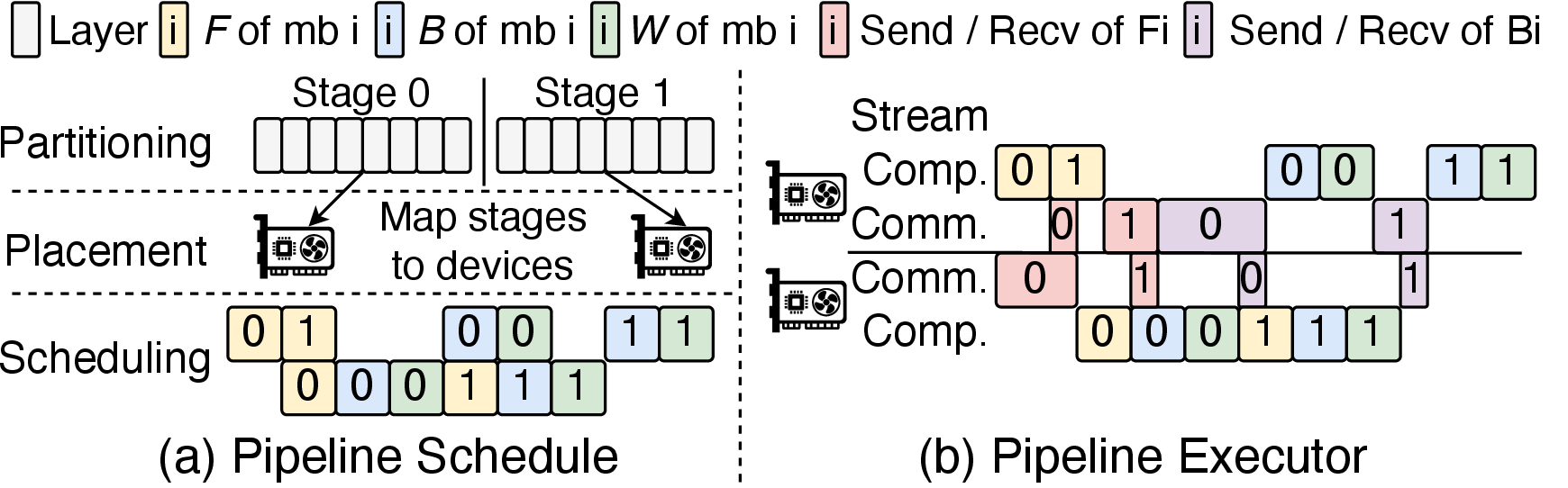
Pipeline Parallelism (PP) [3] typically involves three design phases: partitioning, placement, and scheduling (1 (a)). (1) The partitioning phase determines how the model is divided into stages, each consisting of consecutive model layers. (2) The placement phase determines how these stages are mapped to devices, thereby establishing inter-device data dependencies. Intermediate results are transmitted via point-to-point (P2P) communication between devices hosting dependent stages. (3) The scheduling phase determines the execution order of micro-batches across stages for forward and backward passes. Each phase admits multiple policies, and different combinations of these policies lead to different pipeline schedules. A pipeline executor then runs the training process according to the chosen pipeline schedule. We next introduce these three phases and the pipeline executor.
2.2 Pipeline Phases↩︎
Partitioning. A common partitioning strategy is to evenly divide model layers across stages, with the input layer assigned to the first stage and the output layer to the final stage [2], [9], [11], [28], [31], [35]. Recent approaches adjust the number of layers per stage [23]–[26]. These approaches formulate the partitioning task as an Integer Linear Programming (ILP) problem, which is solved through dynamic programming [25], [26] or ILP solvers [36], [37]. While these approaches mitigate imbalance to some extent, bubbles remain substantial while training heterogeneous models (3).
Placement. A widely adopted strategy is to sequentially map the stages to devices [9]–[11], [24]–[26], [31], assuming the number of stages equals the PP size. Interleaved [2] introduces virtual stages, which split stages into smaller ones, to reduce bubbles at the beginning and end of the pipeline (i.e., boundary bubbles). Hanayo [28] builds upon this idea but applies a wave-like stage-to-device mapping strategy. Chimera [29] duplicates stages to form multiple pipelines, enabling concurrent execution of multiple micro-batches, at the cost of additional memory overhead. However, these placement strategies primarily target homogeneous models. On heterogeneous models, imbalanced computation across stages may introduce bubbles.
Scheduling. Scheduling determines the execution order of micro-batches. With backward splitting [4], [31], [38], [39], the backward pass is further decomposed into input gradient computation (\(B\)) and parameter gradient computation (\(W\)), enlarging the scheduling space. Existing scheduling policies can be broadly categorized into two paradigms. The first adopts fixed scheduling policies (e.g., GPipe [3], DualPipe [4], and Interleaved [2]), which rely on predefined execution orders. While efficient, these approaches lack the flexibility to adapt to heterogeneous models. The second formulates scheduling as an optimization problem and uses ILP solvers to derive execution orders (e.g., ZeroBubble [31], DynaPipe [11], and Tessel [30]). Although more flexible, these approaches suffer from poor scalability due to the rapidly growing search space with increasing numbers of layers, stages, and micro-batches (13). Furthermore, they typically assume fixed partitioning and placement, preventing joint optimization.
| Tuning | ||||
| Tuning | ||||
| Tuning | ||||
| Mist [23] | ||||
| Alpa [24] | ||||
| Dapple [9] | ||||
| AdaPipe [25] | ||||
| Metis [26] | ||||
| Interleaved [2] | ||||
| DualPipe [4] | ||||
| Hanayo [28] | ||||
| Chimera [29] | ||||
| Tessel [30] | ||||
| DynaPipe [11] | ||||
| ZeroBubble [31] | ||||
| Mario [40] | ||||
| (Ours) |
2.3 Pipeline Executor↩︎
The pipeline executor orchestrates computation and communication on each device to materialize a pipeline schedule (1 (b)). Prior executor designs tightly couple execution logic with specific phase policies [2], [3], [9], [11], assuming fixed and regular execution orders. Specifically, the 1F1B executor enforces a fixed execution order that repeatedly performs receive, forward/backward, and send operations on each device [41], tailored to the 1F1B pipeline schedule [9].
However, this tight coupling limits their ability to adapt to irregular execution orders and prevents them from directly supporting new phase designs without modifying the executor logic. For example, Interleaved [2] modifies the execution order of 1F1B to support virtual stages, while DynaPipe [11] implements multiple executors for supporting different scheduling policies. As a result, such executors cannot natively support co-optimized pipelines, which induce irregular execution orders that violate the phase-specific execution order assumptions in existing executors
3 Motivation↩︎
![Figure 2: [Motivation] (a) Nemotron-9B [15] shows a higher bubble ratio than GPT-13B [14] with 1F1B [9], four stages, eight micro-batches, 4k sequence length, and four H800 GPUs. (b) Computation costs of different layer types in Nemotron-9B. (c) Imbalanced computation across stages in Nemontron-9B.](/article/2509.23722/Figures/combined_1f1b_heter_bubble.png "fig:")
3.1 Increasing Model Heterogeneity Amplifies Bubbles↩︎
Homogeneous models [5], [12], [14] are composed of a single layer type. For example, GPT [14] stacks identical Transformer layers [21]. In contrast, heterogeneous models [4], [6], [7], [15]–[17], [19] combine multiple layer types. For instance, Nemotron [15] alternates Mamba [20], Self-Attention, and MLP layers. We measure the bubble ratios on different models with the widely used 1F1B schedule [9], four stages, eight micro-batches, and four H800 GPUs. 2 (a) shows that the more heterogeneous Nemotron-9B [15] exhibits a substantially higher bubble ratio than GPT-13B [14]. This arises because different layer types have different computation costs, as shown in 2 (b). In pipeline parallelism, these differences translate into significant inter-stage latency variance. 2 (c) further illustrates how this variance amplifies pipeline bubbles. Specifically, the maximum inter-stage computation-time gap is about 200 ms in GPT [14] but exceeds 1800 ms in Nemotron [15]. This severe imbalance makes the slowest stage a straggler, causing faster stages to idle while waiting [42] and increasing the maximum bubble ratio from 21.4% to 53.8%. These results show that increasing model heterogeneity can substantially degrade pipeline efficiency, making bubble reduction increasingly important.
![Figure 3: [Motivation] A brief illustration of tuning the 1F1B pipeline schedule for a heterogeneous model with two stages (S0 and S1) and two micro-batches. Subfigures (b-d) show the benefit of tuning a single phase. Subfigure (e) shows the benefit of co-optimizing. F denotes the forward pass, and the backward pass is split into B and W.](/article/2509.23722/Figures/3_co_opt.png "fig:")
3.2 Reducing Bubbles Demands Co-optimizing Pipelines↩︎
In 3 (a), we consider training a heterogeneous model with two stages, where S0 requires 2T for each computation workload (e.g., \(F\), \(B\), and \(W\)) and S1 requires 4T due to different layer types, two micro-batches, 1F1B pipeline [32].
Limited Bubble Reduction of Prior Approaches. Prior approaches summarized in 1 typically optimize only a single pipeline phase. As illustrated in 3 (b–d), although these approaches reduce bubbles by up to 4T, a substantial amount of bubble time remains. Specifically, tuning partition balances computation workloads on S0 and S1 (3 (b)), but leaves the bubbles at the beginning and end of S1 unresolved. While tuning placement reduces these bubbles, the computation workloads on S0 and S1 remain imbalanced (3 (c)). Tuning scheduling primarily reduces bubbles on S1, whereas bubbles on S0 persist (3 (d)). These examples suggest that optimizing any single phase is insufficient, leaving substantial optimization headroom unexplored (see 10).
Unlocking Optimization Headroom with Co-Optimization. 3 (e) presents a case study of jointly optimizing the partition, placement, and scheduling of the 1F1B [9] pipeline. In this example, we apply three optimizations on partition, placement, and scheduling, respectively: (1) moving layers from stage 1 to stage 0, (2) splitting the original two stages into six virtual stages, and (3) reordering the execution of the 1F1B pipeline. Combining these optimizations for partition, placement, and scheduling reduces the pipeline execution time by 10T (\(\approx\)33%), substantially reducing pipeline bubbles. This case study highlights the significant optimization headroom unlocked by co-optimization.
![Figure 4: [Motivation] (a) The naive coordination of computation, send, and receive operations. (b) A deadlock caused by naive coordination. (c) Execution orders without overlap. (d) Reordering computation and communication operations to prevent deadlocks and reduce bubbles with overlap.](/article/2509.23722/Figures/3_deadlock_bubble.png "fig:")
3.3 Co-optimizing Pipelines Remains Challenging↩︎
Complex Pipeline Performance Modeling. Accurately evaluating pipeline performance under diverse partitioning, placement, and scheduling choices is fundamental to co-optimization. However, changing any of these phases alters the computation, communication, and memory-access patterns across GPUs. These changes affect the degree of computation–communication overlap, pipeline bubbles, and memory footprint. As a result, modeling pipeline performance with high fidelity is inherently difficult, making accurate performance estimation a major obstacle to effective co-optimization.
Combinatorial Co-Optimization Search Space. Given a model with \(L\) layers, \(S\) stages, \(N\) GPUs, and \(M\) micro-batches, jointly optimizing partitioning, placement, and scheduling yields a combinatorial search space. In particular, the number of partitioning choices is \(\binom{L-1}{S-1}\). Assigning \(S\) stages to \(N\) GPUs introduces \(N^S\) placement choices. Furthermore, with \(M\) micro-batches, the number of valid scheduling choices is \(\frac{(2M)!}{2^M}\), since the backward pass of each micro-batch must occur after its forward pass. The resulting design space is therefore on the order of \(\binom{L-1}{S-1} \times N^S \times \frac{(2M)!}{2^M}\). Such a combinatorial space makes exhaustive exploration infeasible, necessitating an efficient co-optimization algorithm.
Irregular Execution Orders. Co-optimization can generate irregular orders of computation and communication, violating the regular execution-order assumptions made by prior executors [9], [11], [31]. As discussed in §2.3, supporting such schedules requires a more flexible executor. Moreover, without careful coordination, these irregular orders can lead to deadlocks or bubbles. The naive coordination (4 (a)) that places a receive operation before computation and a send operation after computation can lead to deadlock when two devices concurrently issue send (or receive) operations (4 (b)) [43], [44]. Moreover, directly executing such orders may serialize computation and communication, eliminating potential overlap and introducing bubbles (4 (c)). Avoiding deadlocks and reducing bubbles requires carefully coordinating computation and communication across stages (4 (d)). However, co-optimization may generate a large number of unpredictable execution orders, making static coordination insufficient. Consequently, the executor must dynamically reorder computation and communication to avoid deadlocks and maximize overlap.
4 OctoPipe System Overview↩︎
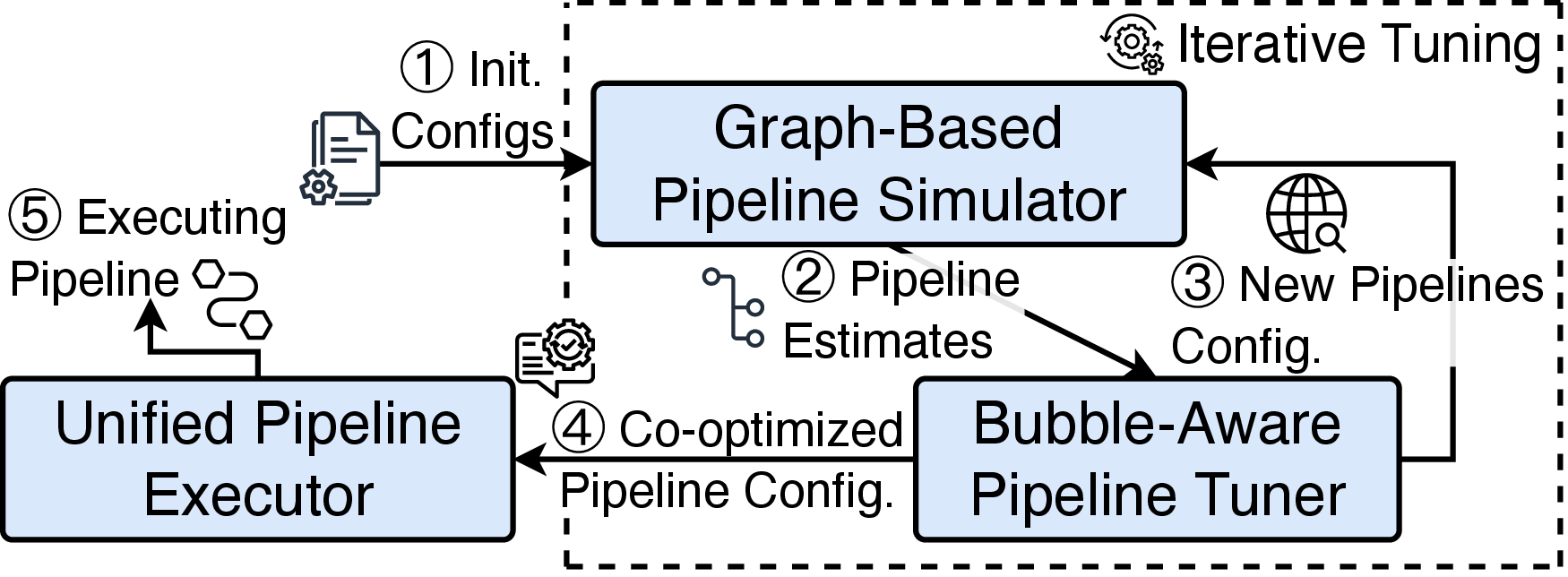
5 illustrates the overall workflow of OctoPipe. OctoPipe takes as input offline profiled statistics (e.g., communication cost, per-layer computation cost, and memory usage), training
configurations (e.g., #micro-batches, #layers, and layer types), and pipeline configurations (i.e., partition, placement, and scheduling). The graph-based pipeline simulator (§5) constructs a DAG with these
inputs and traverses the graph to simulate pipeline execution (e.g., forward, backward, send, and receive operations) and estimate performance metrics, including computation time, communication time, bubble time, and memory footprint. Guided by these
estimations, the bubble-aware pipeline tuner (§6) iteratively refines the partition, placement, and scheduling policies to explore better pipelines. Once the search terminates, the unified pipeline executor (§7) adaptively reorders computation and communication operations to maximize computation-communication overlap, and executes the pipeline. OctoPipe operates at the PP level and is orthogonal to other
parallelism schemes [18], [45], as well
as memory-saving techniques [46]–[50].
5 Graph-Based Pipeline Simulator↩︎
Simulating Pipeline Execution. Given the input configurations, the simulator models pipeline execution as a DAG. 6 (a) illustrates a DAG representation of a pipeline execution with two stages and two micro-batches on two GPUs. Each DAG node represents one of three types of operations: (1) computation nodes for forward and backward passes of micro-batches, (2) communication nodes for send and receive operations, and (3) memory nodes for allocating and releasing intermediate tensors. Each computation or communication node is associated with a memory node. Edges in the DAG capture data dependencies between operations.
Modeling Cross-Phase Interactions. The simulator updates the corresponding node attributes (6 (b)) in the DAG to model cross-phase interactions when pipeline phases change. Changes to one phase
(partitioning, placement, or scheduling) often propagate to the others, coupling computation, communication, and memory behaviors across phases and complicating accurate pipeline performance estimation. Such interactions are difficult to capture with
closed-form analytical models [23], [24], [26]. In particular, altering partitioning changes the distribution of computation and memory across stages, placement changes the communication pattern between devices, and scheduling changes the execution order and overlap
between computation and communication. To capture these effects, the simulator adjusts the modules, stime (start time), and etime (end time) of computation nodes and the mem_cost of memory nodes to
reflect partitioning changes. For placement changes, the simulator inserts or removes communication nodes corresponding to inter-device data dependencies. For scheduling changes, the simulator modifies the execution order of computation and communication
nodes. The simulator naturally extends to support memory optimization techniques [46], [48], which can be seamlessly modeled by adjusting the stime and etime of computation nodes and the mem_cost of memory nodes.
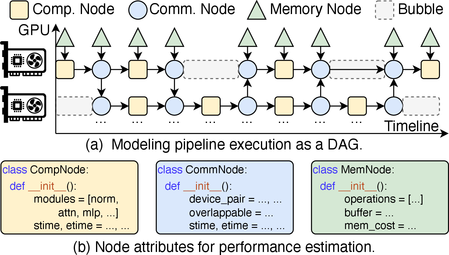
Estimating Pipeline Performance. The simulator traverses the DAG and accumulates timing and memory usage on each device to derive performance metrics. During traversal, it records the start and end time of each node and treats any idle
period on a device as bubble time. For communication nodes, the simulator determines whether send or receive operations can overlap with subsequent computation. If so, it marks them as overlappable and records the minimum of the computation
and communication durations as the overlap time. Using the recorded timing and memory information, the performance model derives metrics including computation time, communication time, memory usage, bubble time, and computation–communication overlap time.
These metrics guide the pipeline tuner in exploring the co-optimization search space.
6 Iterative Bubble-Aware Pipeline Tuner↩︎
OctoPipe employs an iterative tuning algorithm to efficiently explore the combinatorial search space of co-optimizing partitioning, placement, and scheduling. At each iteration, the tuner estimates the potential for bubble reduction in the
pipeline and adjusts the phase that is most likely to reduce bubbles. The process repeats until no further performance improvement is observed for several iterations.
Optimization Objective. The goal of the tuner is to minimize the pipeline execution time. Let \(\mathcal{D}\) denote the set of devices in the pipeline. \(T_d^{\text{execution}}\) denotes the execution time of device \(d \in \mathcal{D}\), and the pipeline execution time is defined as \[T^{\text{pipeline}} = \max_{d \in \mathcal{D}} T_d^{\text{execution}} .\]
The tuner optimizes the input partitioning, placement, and scheduling to minimize \(T^{\text{pipeline}}\). Let \(L\) denote the number of layers, \(S\) the number of stages, \(R\) the number of pipeline ranks, and \(M\) the number of micro-batches. The partitioning is represented by a vector \(\mathbf{P} \in \mathbb{Z}_{+}^{S}\), where \(p_s\) denotes the number of layers assigned to stage \(s\) and \(\mathbf{1}^{\top}\mathbf{P} = L\). The placement is represented by a collection \(\mathbf{A} = \{A_r \mid r \in \{1,\dots,R\}\}\), where \(A_r \subseteq \{0,\dots,S-1\}\) denotes the set of stages assigned to rank \(r\) and \(A_r \cap A_{r'} = \emptyset \; (r \ne r'), \bigcup_{r=1}^{R} A_r = \{0,\dots,S-1\}.\) The scheduling is represented by \(\mathbf{O} = \{O_r \mid r \in \{1,\dots,R\}\}\), where \(O_r \in \{fwd,bwd,send,recv\}^{M \cdot |A_r|}\) denotes the sequence of operations executed on rank \(r\). Here \(fwd\), \(bwd\), \(send\), and \(recv\) represent forward, backward, send, and receive operations. The optimization problem is formulated as \[\begin{align} \min_{\mathbf{P},\,\mathbf{A},\,\mathbf{O}} \quad & T^{\text{pipeline}} = \max_{d \in \mathcal{D}} T_d^{\text{execution}} \\ \text{s.t.}\quad & M_d^{\text{peak}} \le M_d^{\text{capacity}}, \quad \forall d \in \mathcal{D}. \end{align}\]
Iterative and Bubble-Aware Tuning. We develop an iterative and bubble-aware tuning 8 to efficiently explore the large co-optimization search space. In each iteration, the tuner optimizes the three phases with the following priorities: (1) partitioning, to balance workloads across devices; (2) placement, to reduce boundary bubbles; and (3) scheduling, to minimize residual bubbles. This priority order is motivated by our empirical observation that workload imbalance is the dominant source of bubbles. Once workloads are balanced across devices, the bubbles at the pipeline boundaries account for most of the remaining bubbles. After addressing these two sources, scheduling optimization can further reduce residual bubbles. Changing this priority order leads to slower convergence or produces worse pipelines under the same tuning time budget (see 13). This iterative strategy decomposes the joint optimization into a sequence of phase-level bubble reductions, substantially shrinking the effective search space and producing efficient pipeline schedules.
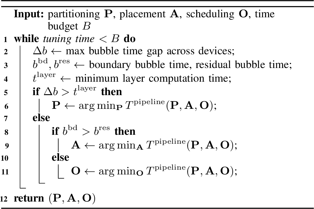
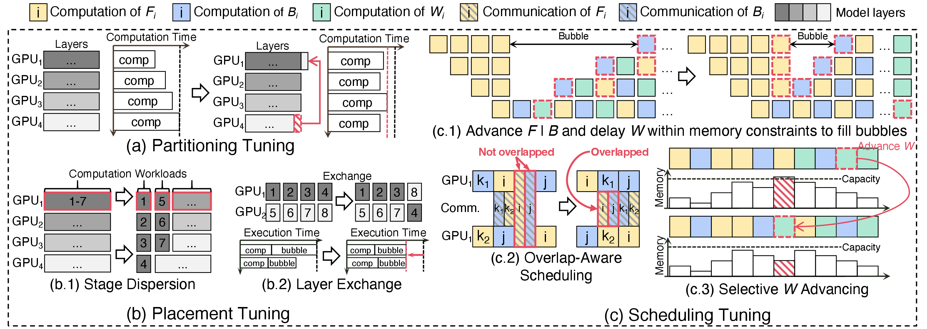
Partitioning Tuning. The tuner adjusts the number of layers per device to balance workloads across devices. 7 (a) illustrates the partitioning tuning procedure. First, the tuner fetches the workload estimate on each device from our simulator. Second, the tuner migrates layers from the most loaded device to the least loaded device to reduce imbalance. Third, the tuner modifies the DAG and calls the simulator to reevaluate the new partitioning. This migrate-and-reevaluate process repeats until no better partitioning can be found.
Placement Tuning. The tuner employs two policies to tune placement: stage dispersion and layer exchange. The stage dispersion refines the granularity of computation workloads. As shown in 7 (b.1), the tuner first identifies stages that contain multiple layers, then splits such a stage into individual layers and assigns them to different devices. The stage dispersion reduces the number of layers per stage, yields finer-grained stages, and decreases bubbles at the beginning and end of the pipeline. The layer exchange balances computation time and bubble time to minimize overall execution time. 7 (b.2) illustrates the layer exchange process. When \(\text{GPU}_1\) and \(\text{GPU}_2\) have comparable computation workloads but \(\text{GPU}_1\) experiences longer bubble time, the tuner selects a layer from \(\text{GPU}_1\) and a more compute-intensive layer from \(\text{GPU}_2\) to swap. This exchange trades computation time for reduced bubble time, lowering the overall execution time.
While fine-grained stages reduce boundary bubbles, they introduce additional communication overhead. We mitigate this through overlap-aware scheduling (7 (c.2)) and execution (§7), which hide communication latency by overlapping it with computation (see 2).
Scheduling Tuning. The tuner employs three policies to tune the scheduling. First, in 7 (c.1), the tuner advances \(F\) and \(B\), and delays \(W\) within the memory constraints to fill bubbles. This policy is motivated by the fact that both \(F\) and \(B\) exhibit inter-device data dependencies that can induce bubbles, whereas \(W\) does not. For instance, the \(F\) on stage \(i\) depends on the result from stage \(i-1\), and the \(B\) on stage \(i\) depends on the result from stage \(i+1\). \(W\) has no inter-device data dependencies since it relies only on \(B\) on the same device. This policy has two merits: (1) executing \(F\) and \(B\) earlier releases more \(W\) in the following scheduling, and (2) the deferred \(W\) can be scheduled to fill bubbles in cases where \(F\) and \(B\) cannot do so due to data dependency.
Second, the tuner employs an overlap-aware scheduling policy to hide communication overhead. This policy inserts other computations to overlap with communications that were previously non-overlappable due to data dependencies. In 7 (c.2), the communication of \(F_i\) cannot initially overlap with its own computation because of a data dependency, but \(B_{k_1}\) has no dependency on the communication of \(F_i\). To exploit this, the tuner inserts \(B_{k_1}\) between \(F_i\) and \(B_j\) on GPU1. Similarly, it inserts \(B_{k_2}\) between \(B_j\) and \(F_i\) on GPU2. After rescheduling, the communications of both \(F_i\) and \(B_j\) are overlapped with the computations of \(B_{k_1}\) and \(B_{k_2}\).
Third, the tuner leverages a selective \(W\) advancing policy to prevent OOM errors. For each scheduling, the tuner calls the simulator to locate memory peak usages. As shown in 7 (c.3), if the peak memory exceeds device capacity, the tuner advances the computation of some workload’s \(W\) to lower the peak. It first searches for a \(W\) whose advancement does not increase bubble time; if none exists, it advances the earliest eligible workload instead. This process repeats until the peak memory on every device fits within its capacity.
7 Unified Pipeline Executor↩︎
We design a unified pipeline executor that supports irregular execution orders while preventing deadlocks and maximizing computation-communication overlap.
Supporting Irregular Execution Orders. As analyzed in §2.3, prior executors [2], [9], [11] enforce fixed computation and communication orders tailored to specific phase designs, making them ill-suited for the irregular schedules generated by co-optimization. In contrast, our executor does not rely on predefined phase-specific execution patterns, and instead derives execution orders directly from a pipeline DAG produced by our simulator (§5). The DAG consists of nodes and edges: each node represents an operation (e.g., forward, backward, send, or receive), and each edge encodes an execution dependency. Partitioning, placement, and scheduling only modify the DAG structure and node attributes, which together determine the execution order of operations on each device. Ignoring communication stalls caused by inter-device data dependencies, the executor can directly follow this derived order to execute arbitrary irregular pipeline schedules.
Deadlock-Free and Overlap-Aware Reordering. However, the communication stalls might incur deadlocks, discussed in §3.3. Specifically, when multiple devices simultaneously issue send
or recv, they may form cyclic waiting dependencies, leading to deadlock [11], [43]. We propose to reorder communication operations to break such cyclic dependencies. However, reordering changes the DAG and may thereby introduce additional pipeline bubbles.
To address this issue, we design a deadlock-free, overlap-aware reordering policy that eliminates communication deadlocks while reducing pipeline bubbles. The policy consists of three steps. First, given the DAG, the executor traverses all communication
operations and identifies mismatched send/recv pairs across devices that may lead to cyclic dependencies. This step takes \(O(|V_c|)\) time, where \(|V_c|\) is the
number of communication nodes. Second, for each mismatched pair, the executor locates its dependent computation nodes and derives a feasible insertion window based on their execution intervals. This window bounds the valid positions where the communication
can be reordered, effectively restricting the search space to a small local region. Within the feasible window, the executor enumerates candidate insertion positions for the corresponding communication nodes. Let \(k_i\)
denote the number of candidate positions for the \(i\)-th communication pair; the overall search complexity is \(O(\sum_i k_i)\). Third, for each candidate schedule, the executor evaluates a
scheduling cost defined as the communication span, i.e., the time interval between the reordered send and recv, minus the overlap achievable with neighboring computation. The executor then greedily selects the minimum-cost
candidate for each communication pair and immediately applies the reordering. Overall, this policy enables the executor to resolve deadlocks while maximizing computation-communication overlap.
![Figure 9: End-to-End throughput (TGS) results across homogeneous and heterogeneous models (normalized to 1F1B [9]).](/article/2509.23722/Figures/e2e_performance.png "fig:")
8 Evaluation↩︎
Evaluation Setup. We implement OctoPipe atop Megatron-LM [32] v0.15.0 in 10k lines of Python code.
We run all experiments on a 16-node cluster with 128 NVIDIA H800 GPUs. Each node has 8 GPUs connected by 200 GB/s NVLink, and nodes are connected by an 8\(\times\)200 Gbps RoCEv2 network. We evaluate OctoPipe
on multiple sizes of LLaMA [5], Jamba [17], and Nemotron-H [19] (see ¿tbl:tab:model95config?).
c@c@c@c@c@c@c Model & Size & \(L\) & \(V\) & \(H\) & FFN Type & Attn. Type
& Small & 32 & 128k & 1536 & FFN & SA
& Medium & 64 & 256k & 1536 & FFN & SA
& Large & 128 & 512k & 1536 & FFN & SA
& Small & 16 & 64k & 2048 & FFN+MoE & SA+Mamba
& Medium & 32 & 128k & 2048 & FFN+MoE & SA+Mamba
& Large & 64 & 256k & 2048 & FFN+MoE & SA+Mamba
& Small & 56 & 128k & 1024 & FFN & SA+Mamba
& Medium & 112 & 256k & 1024 & FFN & SA+Mamba
& Large & 224 & 512k & 1024 & FFN & SA+Mamba
Baselines. We evaluate OctoPipe against the following baselines: (1) 1F1B [9] and (2)
Interleaved [2], as implemented in Megatron-LM with native communication optimizations;
(3) Tessel [30], which adaptively reschedules workloads to minimize bubbles; and (4) Mist [23], an automatic training framework with adaptive partitioning based on dynamic programming. We apply backward splitting [31] uniformly to all baselines as an orthogonal optimization to improve their throughput. We evaluate Tessel over all predefined configurations in its
implementation and report the best observed throughput. To preserve training accuracy [10], [31], we adopt synchronous pipeline execution for all approaches.
Training Configurations. We search for the best parallelism configuration for 1F1B [9] and apply it to all baselines and
OctoPipe. Specifically, TP size is set to 8 and PP size to 4, 8, and 16 for small, medium, and large models, respectively. The number of micro-batches is set to twice the PP size to saturate the pipeline. Unless otherwise noted, we set the
sequence length to 4k. Training throughput results are measured with average Tokens/GPU/Second (TGS) in the first 100 iterations.

8.1 End-to-End Evaluation↩︎
Throughput Results on Heterogeneous Models. In 9, OctoPipe consistently delivers the highest end-to-end training throughput across Jamba and Nemotron-H models, achieving 1.23\(\times\)–1.44\(\times\), 1.21\(\times\)–1.38\(\times\), 1.17\(\times\)–1.40\(\times\), and 1.15\(\times\)–1.20\(\times\) speedups over 1F1B, Interleaved, Tessel, and Mist, respectively. These gains arise from joint optimization of
partitioning, placement, and scheduling, enabled by a unified executor. Interleaved reduces boundary bubbles by introducing virtual stages, effectively improving placement. However, it does not address stage imbalances, which are the dominant source of
bubbles, nor does it enable effective scheduling to eliminate residual bubbles, providing modest improvements over 1F1B (1.02\(\times\)–1.05\(\times\)). Tessel tunes scheduling via
reordering execution. However, without mitigating stage imbalance through partitioning or exposing sufficient scheduling opportunities via placement, it yields limited improvements (1.03\(\times\)–1.05\(\times\)). Mist alleviates workload imbalance through partitioning, addressing the primary source of bubbles. However, without complementary optimizations on placement and scheduling, bubbles in the boundary and middle of the
pipeline remain, leaving it 12%–25% slower than OctoPipe. These results show that: (1) optimizing any single phase of the pipeline is insufficient for heterogeneous models, and (2) co-optimization effectively reduces bubbles.
Impact of Model Heterogeneity on Throughput. The benefits of OctoPipe become more pronounced as model heterogeneity increases. On LLaMA models, where identical layers lead to well-balanced workloads across stages, the
opportunity for further optimization is inherently limited. As a result, OctoPipe achieves moderate gains (1.14\(\times\)–1.17\(\times\)). In contrast, Jamba and Nemotron-H
models exhibit diverse layer types with varying computation costs, leading to pronounced stage imbalance. By jointly optimizing partitioning, placement, and scheduling, OctoPipe effectively mitigates these inefficiencies, resulting in larger
throughput gains (1.23\(\times\)–1.33\(\times\) on Jamba and 1.26\(\times\)–1.44\(\times\) on Nemotron-H).
Communication and Overlap Analysis.
| Method | #Stages | #Comm. | #Overlap | Overlap Rate | TGS |
|---|---|---|---|---|---|
| 1F1B | 4 | 48 | 24 | 50.0% | 1656 |
| Mist | 4 | 48 | 24 | 50.0% | 1822 |
| Tessel | 8 | 96 | 64 | 66.7% | 1740 |
| Interleaved | 56 | 880 | 665 | 75.6% | 1738 |
| OctoPipe | 56 | 880 | 803 | 91.3% | 2087 |
2 reports communication volume and overlap statistics for Nemotron-H (Small). Increasing the number of stages leads to higher communication volume, but improved communication–computation overlap effectively hides
this overhead. As a result, Tessel, Interleaved, and OctoPipe all achieve higher throughput than 1F1B, despite substantially increased communication. These results highlight the importance of overlap-aware scheduling; OctoPipe
further benefits from its executor support to realize such overlap efficiently.
Bubble Reduction Analysis. 10 compares the profiled traces of 1F1B and OctoPipe on Nemotron-H (Small). OctoPipe significantly reduces bubbles through co-optimization, as
indicated by the much smaller red regions in 10 (b) than in 10 (a). This improvement stems from (i) better workload balance across GPUs via tuning partitioning, (ii) fine-grained placement
that reduces boundary bubbles, and (iii) more effective scheduling that increases computation–communication overlap and fills bubbles. These effects collectively shorten the end-to-end execution time.
Despite these improvements, marginal bubbles persist. First, a fraction of communication (approximately 8.7% in 2) remains unoverlapped due to inherent data dependencies, even with our overlap-aware designs. Second, the DAG-driven executor can deviate from the original schedule under runtime variability (e.g., network jitter and hardware performance fluctuations), introducing additional inefficiencies. Nevertheless, these overheads are minor in practice and are outweighed by the gains from the co-optimization.
| Method | Seqlen=2k | 4k | 8k | 16k |
|---|---|---|---|---|
| 1F1B | 925 (1.00\(\times\)) | 1656 (1.00\(\times\)) | 2687 (1.00\(\times\)) | 3755 (1.00\(\times\)) |
| Interleaved | 965 (1.04\(\times\)) | 1740 (1.05\(\times\)) | 2818 (1.05\(\times\)) | 3960 (1.05\(\times\)) |
| Tessel | 981 (1.06\(\times\)) | 1738 (1.05\(\times\)) | 2735 (1.02\(\times\)) | 3821 (1.02\(\times\)) |
| Mist | 1000 (1.08\(\times\)) | 1822 (1.10\(\times\)) | 2982 (1.11\(\times\)) | 4281 (1.14\(\times\)) |
| OctoPipe | 1135 (1.23\(\times\)) | 2087 (1.26\(\times\)) | 3450 (1.28\(\times\)) | 4971 (1.32\(\times\)) |
Impact of Sequence Lengths. 3 shows that OctoPipe consistently outperforms all baselines across evaluated sequence lengths on Nemotron-H (Small). Notably, the TGS improvement of
OctoPipe over the 1F1B becomes more pronounced with increasing sequence length. Longer sequences amplify computational discrepancies across layers, which exacerbates stage imbalances. OctoPipe effectively mitigates these
imbalances via co-optimization, yielding increasingly significant gains. Overall, these results demonstrate that OctoPipe adapts effectively across sequence lengths, highlighting its robustness under varying input lengths.
8.2 Performance Breakdown of OctoPipe↩︎
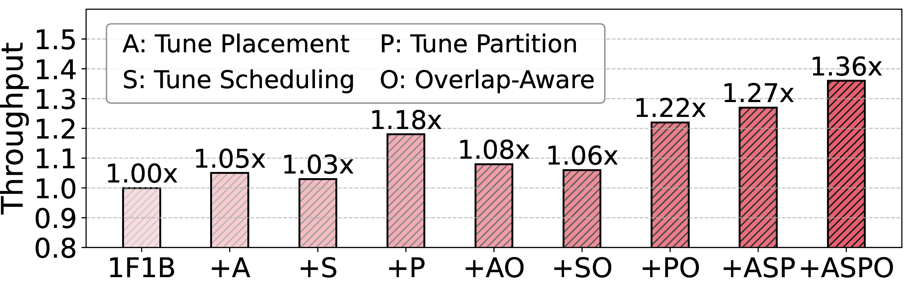
11 shows the performance impact of applying individual and combined optimizations on top of 1F1B for Nemotron-H (Medium). Applying co-optimization (+ASP), OctoPipe achieves 1.27\(\times\) higher training throughput over 1F1B, while incorporating the overlap-aware executor (+ASPO) further improves throughput to 1.36\(\times\). In contrast, applying placement (+A),
scheduling (+S), or partitioning (+P) alone yields 5%, 3%, and 18% improvement, respectively. This result highlights that, in heterogeneous models, workload imbalance across stages is the primary source of bubbles. Partition tuning (+P), which directly
mitigates such imbalances, provides the largest individual gain. However, without complementary placement and scheduling optimizations, residual bubbles remain. The overlap-aware executor (+O) consistently improves throughput across configurations (e.g.,
+AO, +SO, +PO), and delivers the largest gain when combined with co-optimization (+ASPO). This is because it explores execution orders that maximize communication-computation overlap, while co-optimization exposes more opportunities for such overlap.
Overall, these results demonstrate that addressing bubbles requires both co-optimizing and exploiting overlap via the executor.
8.3 Performance Model Fidelity↩︎
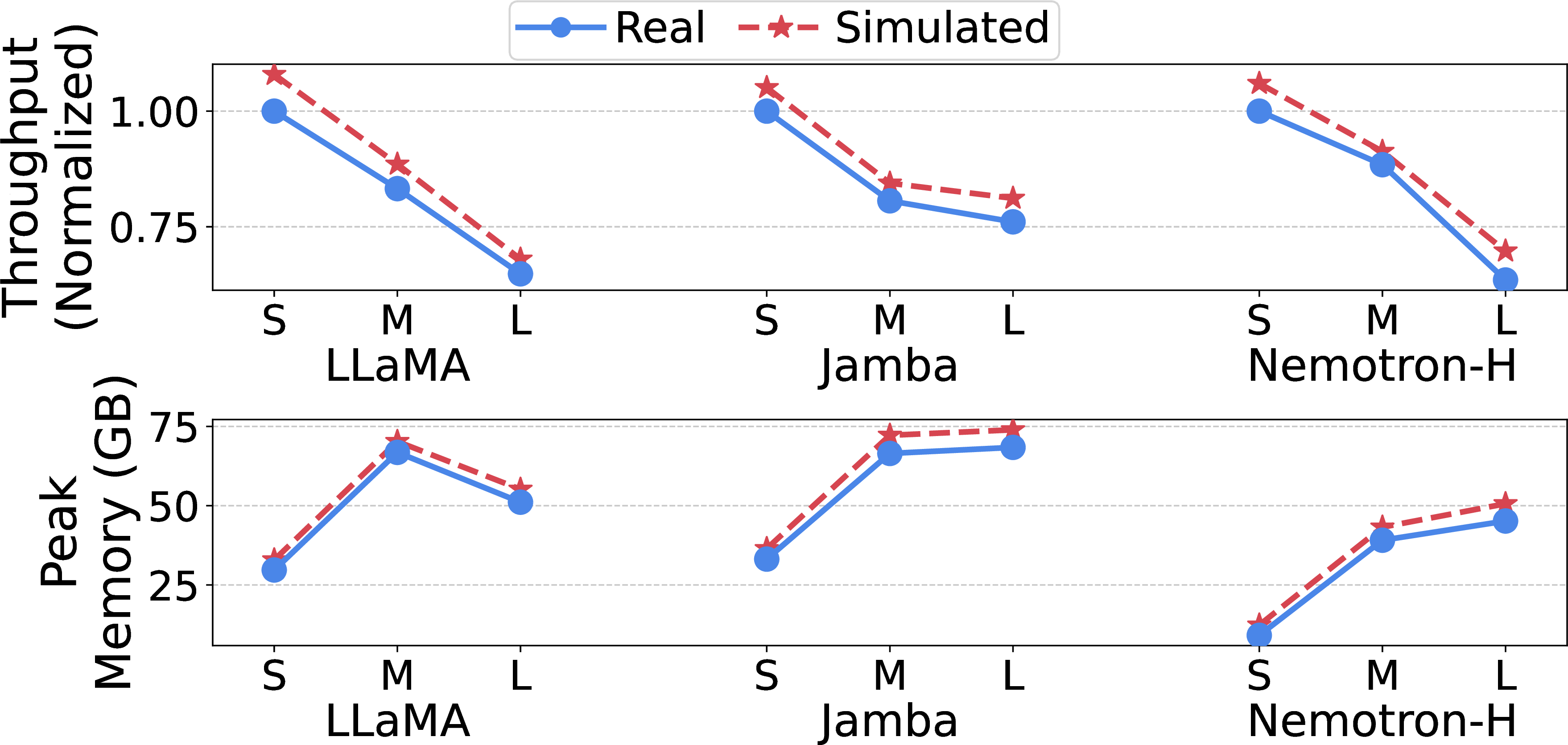
12 shows that OctoPipe simulator (§5) achieves an average prediction error of 5.06% for throughput and 5.29% for peak memory. For throughput, the prediction
error primarily stems from the gap between idealized simulation and real system execution. The simulator assumes deterministic execution times for both computation and communication, while actual runs exhibit performance variability due to hardware-level
noise and runtime fluctuations. For example, in Nemotron-H (Small), two identical Mamba layers exhibit profiled execution times of 2.58 ms and 2.67 ms (a 4% difference), leading to small imbalances that are not captured by the simulator. For memory, the
simulator slightly overestimates peak memory usage because it relies on theoretical upper bounds to ensure safety against OOM errors. Specifically, the simulator does not model certain runtime memory optimizations, such as early release of communication
buffers and activation tensors, which reduce memory usage in practice. As a result, the predicted peak memory is slightly higher than the measured values.
8.4 Pipeline Search Cost↩︎
Iterative Search Efficiency. 13 compares the search processes of OctoPipe, random search, and ILP-based search [30], [31] on Nemotron-H (Large). OctoPipe adopts iterative bubble-aware tuning
(§6), while random search follows the same iterative framework but selects tuning phases randomly without considering bubble characteristics. ILP-based search relies on commercial solvers [36] to jointly optimize the pipeline schedule. Due to the combinatorial search space, ILP-based methods (e.g., Tessel [30]) fail to produce a feasible solution within the same time budget. In contrast, both OctoPipe and random search quickly obtain feasible solutions and continuously refine them
through iterative tuning, demonstrating the efficiency and practicality of the iterative search paradigm.
| Method | Total Iter. | Partitioning | Placement | Scheduling | ||||||||
|---|---|---|---|---|---|---|---|---|---|---|---|---|
| OctoPipe | (100%) | (51.7%) | (34.8%) | (13.5%) | ||||||||
| Random | (100%) | (35.6%) | (31.6%) | (32.8%) |
2pt

Bubble-Awareness Analysis. 4 shows the breakdown of tuning iterations on each phase in 13. Without bubble awareness, random search frequently
optimizes placement and scheduling even when substantial workload imbalance persists across stages. In such cases, the optimization potential of placement and scheduling is inherently limited, as bubbles are dominated by imbalance. In contrast,
OctoPipe prioritizes tuning partitioning early in the search to mitigate workload imbalance. As shown in 4, OctoPipe allocates 165 iterations to partitioning, whereas random search
only allocates 116. This ensures a balanced foundation before the search progressively refines placement and scheduling to reduce boundary bubbles and scheduling to eliminate residual bubbles. This staged, bubble-aware strategy enables
OctoPipe to allocate search time more effectively and achieve superior pipeline schedules than random search.
llccccc & #GPUs & 1F1B & Interleaved & Tessel & Mist & OctoPipe
& 32 & 1656 & 1.05\(\times\) & 1.05\(\times\) & 1.10\(\times\) & 1.26\(\times\)
& 64 & 1540 & 1.04\(\times\) & 1.03\(\times\) & 1.12\(\times\) & 1.29\(\times\)
& 128 & 1388 & 1.05\(\times\) & 1.03\(\times\) & 1.12\(\times\) & 1.30\(\times\)
& 32 & 1656 & 1.05\(\times\) & 1.05\(\times\) & 1.10\(\times\) & 1.26\(\times\)
& 64 & 1570 & 1.04\(\times\) & 1.01\(\times\) & 1.12\(\times\) & 1.24\(\times\)
& 128 & 1438 & 1.03\(\times\) & 1.01\(\times\) & 1.11\(\times\) & 1.23\(\times\)
8.5 Scalability↩︎
¿tbl:tab:scaling95res? presents strong and weak scaling results on Nemotron (Small), measured in Tokens/GPU/Second.
Strong Scaling. OctoPipe consistently outperforms baselines across all GPU scales. We scale the system by increasing the DP size while keeping other configurations unchanged. As the number of GPUs increases, the performance
gap between OctoPipe and prior approaches widens. This is because higher GPU counts reduce per-device memory pressure, enabling OctoPipe to apply more aggressive scheduling optimizations that effectively reduce bubbles.
Weak Scaling. We increase the global batch size proportionally with the number of GPUs to keep the per-GPU workload constant. OctoPipe maintains consistent performance advantages over baselines, although the relative gains
gradually diminish at larger scales. Because a larger batch size increases the number of micro-batches, which reduces the proportion of boundary bubbles in the pipeline and diminishes the impact of placement optimization. In this regime, most of the
remaining bubbles are dominated by workload imbalance, narrowing the performance gap between Mist and OctoPipe.
8.6 Case Study↩︎
| Model | Size | 1F1B | Interleaved | Tessel | Mist | OctoPipe |
|---|---|---|---|---|---|---|
| LLaMA | Large | 78 | 1.07x | 1.08x | 1.08x | 1.12x |
| Jamba | Large | 149 | 1.06x | 1.05x | 1.11x | 1.19x |
| Nemontron-H | Large | 135 | 1.03x | 1.02x | 1.10x | 1.20x |
4pt
| Model | Size | 1F1B | Interleaved | Tessel | Mist | |
|---|---|---|---|---|---|---|
| LLaMA | Large | 1.00\(\times\) | 1.11\(\times\) | 1.18\(\times\) | 1.12\(\times\) | 1.27\(\times\) |
| Jamba | Large | 1.00\(\times\) | 1.07\(\times\) | 1.05\(\times\) | 1.15\(\times\) | 1.33\(\times\) |
| Nemotron-H | Large | 1.00\(\times\) | 1.04\(\times\) | 1.08\(\times\) | 1.24\(\times\) | 1.48\(\times\) |
Large-Scale Simulation. We evaluate OctoPipe in large-scale settings via simulation due to resource limitations. We scale the DP size and proportionally increase the number of micro-batches, while keeping all other
configurations fixed, to emulate training on 8192 GPUs. 5 shows that OctoPipe consistently outperforms baselines, achieving 1.12–1.20\(\times\) higher throughput over
1F1B across models. These results are consistent with the weak scaling trends, indicating that the benefits of OctoPipe persist at large scale.
Incorporating Recomputation. We evaluate OctoPipe with recomputation [46]. As shown in 6, OctoPipe achieves higher speedups over 1F1B with recomputation. This is because reduced memory pressure allows the tuner to explore more effective scheduling choices under relaxed memory
constraints. These throughput improvements also demonstrate that our simulator accurately captures memory dynamics and effectively guides pipeline schedule tuning.
9 Related Work↩︎
Data Heterogeneity. Variations in sequence lengths lead to fluctuations in micro-batch execution time [11], [51]–[53], resulting in bubbles. To mitigate this issue, prior works adopt dynamic strategies such as micro-batch reordering [11], [51], adaptive parallelism [52], and data rebalancing [54]. These approaches primarily target runtime variability induced by input data, rather than heterogeneity within models.
Cross-Model Heterogeneity. Multimodal LLMs combine multiple sub-models to process different modalities, introducing cross-model heterogeneity that leads to bubbles. DistTrain [51] and DISTMM [55] mitigate this by assigning different parallelism configurations to each
sub-model, while DIP [53] distributes layers from each sub-model evenly across stages to balance workloads. Optimus [56] schedules encoder computation to fill bubbles in multimodal LLM training. However, these approaches focus on cross-model heterogeneity. In contrast, OctoPipe
targets intra-model heterogeneity and co-optimizes pipelines to reduce bubbles.
Automatic Parallelization. Automatically identifying efficient parallelization strategies [57]–[61] improves training throughput. Recent approaches [23], [24], [26], [60] optimize partitioning by adjusting the number of layers per stage to reduce bubbles. However, these methods do not consider co-optimization to further reduce bubbles.
Memory Optimizations. Many pipeline systems [23], [25], [40], [50], [62] adopt recomputation [46] and offload [48] to reduce memory overhead. While effective for memory saving, these techniques are largely complementary to OctoPipe.
10 Conclusion↩︎
We present OctoPipe, a pipeline parallelism system that mitigates pipeline bubbles for heterogeneous models. OctoPipe combines a graph-based pipeline simulator for accurate performance estimation with an iterative, bubble-aware
tuner that co-optimizes partitioning, placement, and scheduling. We design a unified pipeline executor with deadlock-free, overlap-aware reordering to avoid deadlocks and maximize computation–communication overlap. Experiments demonstrate that
OctoPipe achieves high simulation accuracy (5.29% average prediction error), enables efficient pipeline schedule search, and improves training throughput by 1.15\(\times\)–1.44\(\times\) compared to state-of-the-art PP systems.
References↩︎
*Equal contribution. Corresponding author.↩︎