Bayesian Transfer Operators
in Reproducing Kernel Hilbert Spaces
September 26, 2025
Abstract
The Koopman operator, as a linear representation of a nonlinear dynamical system, has been attracting attention in many fields of science. Recently, Koopman operator theory has been combined with another concept that is popular in data science: reproducing kernel Hilbert spaces. We follow this thread into Gaussian process methods, and illustrate how these methods can alleviate two pervasive problems with kernel-based Koopman algorithms. The first being sparsity: most kernel methods do not scale well and require an approximation to become practical. We show that not only can the computational demands be reduced, but also demonstrate improved resilience against sensor noise. The second problem involves hyperparameter optimization and dictionary learning to adapt the model to the dynamical system. In summary, the main contribution of this work is the unification of Gaussian process regression and dynamic mode decomposition.
1 Introduction↩︎
Modeling and forecasting the behavior of noisy, high-dimensional, and nonlinear systems remains an active area of research. Yet, the governing laws of these systems are often unknown or prohibitively expensive to simulate. With the proliferation of measurement sensors and the advent of efficient computational hardware, our modern world is abundant with multi-fidelity data that enables us to construct models directly from data without relying solely on first principles. Beyond merely generating predictions, it is also possible to extract interpretable spatio-temporal patterns and coherent structures from the data, thereby deepening our understanding and enhancing our analysis of complex dynamical systems.
Transfer operator theory and reproducing kernel Hilbert spaces (RKHSs) are popular approaches that result in analytically informative algorithms [1]–[9], while also contributing widely to practical applications [10]–[17]. Both Koopman operator and RKHS techniques frame their corresponding problems in a functional analytic setting. Therefore, it stands to reason that by combining methods from both of these two fields, we can design robust algorithms that provide compact and interpretable models for (stochastic) time-series.
1.1 Dynamic Mode Decomposition↩︎
Transfer operators, such as the Koopman and Perron–Frobenius operators, describe the theory of linearizing a dynamical system, not merely around its fixed points, but globally without any approximation. The operator-theoretic perspective is particularly appealing because it is integrated with well-understood statistical and geometric perspectives, which ties in with insights into the physical behavior of dynamical systems mezic2019spectrumkoopmanoperatorspectral?, koopman1931hamiltonian?, koopman1932dynamical?.
The Koopman operator, being an infinite-dimensional object, must often be empirically approximated before it can be implemented on a computer. This involves discretizing the operator and identifying a suitable set of basis functions that span a finite-dimensional subspace wherein the spectral properties of the operator can be represented — a task that falls under the heading of dictionary learning [18]–[24].
One such suite of algorithms that discretizes the Koopman operator is dynamic mode decomposition (DMD; [25]–[27]). DMD can be described as a Galerkin method that blends together principal component analysis (PCA) and the discrete-time Fourier transform [28]. In other words, one may think of DMD as rotating the (lower) dimensional PCA space such that each basis has dynamics oscillating according to a single frequency and a single growth (or decay) rate.
In part, DMD remains attractive because it is based on an eigenvalue decomposition of a model obtained through linear regression. After projecting the system to a higher-dimensional space, DMD can provide accurate models of nonlinear [26], [29] and stochastic systems [30]–[32], vcrnjaric2020koopman?. In other words, all the techniques belonging to linear time-invariant ODEs, such as spectral analysis, multi-step forecasting, numerical simulation, and even control [33], [34], peitz2019koopman?, otto2021koopman? can be readily transferred to nonlinear systems. Moreover, should the system contain a large number of variables (e.g., in fluid dynamics), DMD can facilitate dimensionality reduction.
1.2 Gaussian Process Regression↩︎
Following the authors [29], [35]–[40], das2020koopman?, ikeda2022koopman?, bevanda2024koopman?, bevanda2025koopman?, the underlying machinery of our DMD algorithm is a reproducing kernel function (i.e., a covariance function). Kernel methods are non-parametric, enhance interpretability of features, and are generally more flexible compared to parametric models (e.g., multilayer perceptrons), since they encompass all functions sharing the same degree of smoothness. It is the non-parametric nature of kernel algorithms that grant them the intrinsic ability to implicitly construct a functional basis for a model directly from data. Thereby, they provide a natural choice for the hypotheses space: an RKHS. It is these properties that often lead to strong theoretical performance guarantees [9], [41], [42].
One popular kernel regression framework (for modeling dynamical systems), is Gaussian process (GP) regression [4], [43]–[46]. GP regression is a function approximation technique that is capable of providing accurate estimations of an unknown function based on a limited set of noisy training targets and high-level assumptions about the function. Moreover, a GP model is numerically straightforward to estimate, the predictions of the model are fully probabilistic, and the theory provides a well-founded framework for model selection.
1.3 Contributions of this work↩︎
The core idea is to transfer the attractive features of GP regression to DMD. Thereby, we develop a Bayesian interpretation of the embedded Perron–Frobenius operator [39] which opens up avenues to extend kernel-based DMD algorithms with established sparsity and hyperparameter tuning techniques. The result is a modification of ‘Extended DMD’ (EDMD; [26]) that constructs models from noisy measurement data of a nonlinear dynamical system and provides uncertainty estimates for multi-step predictions.
The remainder of this paper is structured as follows. Section 2 introduces a Bayesian formulation of DMD, and Section 3 explores its mathematical consequences and numerical performance. Lastly, in Section 4, we conclude with some final remarks, open questions, and point toward straightforward extensions. In Appendix 5 we review (sparse) GP regression and the notation of [4], and for convenience and completeness we also present an overview of (kernel) transfer operators [39] in Appendix 6.
2 Gaussian Process Dynamic Mode Decomposition↩︎
Because kernel-based DMD algorithms often quickly become impractical for large data sets due to the high training cost, one of our goals is to apply the variational free energy (VFE) method [47] to kernel Koopman operators [39]. For example, in [39], to estimate the Koopman matrix we need to take the inverse of a Gramian which has a complexity of \(\mathcal{O}(N^3)\), where \(N\) is the number of training samples; moreover, the eigenvalue decomposition also has a complexity of \(\mathcal{O}(N^3)\). Therefore, we are motivated to find a better trade-off between the model’s generalization error and its computational complexity. We want a non-parametric model that automatically adapts to the complexity of the dynamics, but not to the point where all the training inputs define the basis dictionary.
We will demonstrate how our algorithm is a special case of EDMD [26]. Which means that it inherits some of EDMD’s limitations [48]–[50]. This should not be surprising, since it is quite common to derive the same expressions within either a frequentist or Bayesian framework. This duality between ridge-regression and Bayesian models is well-known, and has been pointed out in [4], [51]–[53]. One might then assume that the choice of framework merely reflects an attitude, with each attitude corresponding to a preferred mode of reasoning about how to construct a (data-driven) model. However, we could argue that attitudes matter because they suggest different approaches to improving upon the state-of-the-art. Hence, one of our goals is to shed some light on this debate.
For example, EDMD does not intrinsically provide an optimization scheme for selecting either the hyperparameters or the dictionary, and therefore requires another explicit strategy, e.g., [54]. Neither does EDMD provide uncertainty-aware predictions, nor does it take into account measurement noise from the outset. Our amalgamation of DMD and GP regression wraps up the entire model inference pipeline into one coherent theory that simultaneously addresses hyperparameter optimization and sparse dictionary learning. This naturally raises the question of whether such an approach is overly restrictive and sacrifices the flexibility of frequentist methods.
2.1 Operators as Random Variables↩︎
| Variable | Symbol |
|---|---|
| \(\Z \coloneqq[\bm{z}_1, ..., \bm{z}_M]\) | |
| \(\X \coloneqq[\bm{x}_1, ..., \bm{x}_N]\) | |
| \(\Y \coloneqq[\bm{y}_1, \dots, \bm{y}_N]\) | |
| \(\Phi_Z \coloneqq[ \varphi(\bm{z}_1), ..., \varphi(\bm{z}_M) ]\) | |
| \(\Phi_X \coloneqq[ \varphi(\bm{x}_1), ..., \varphi(\bm{x}_N) ]\) | |
| \(\kappa_{\mathrm{pr}}(\bm{x}, \bm{x}') \coloneqq \langle \varphi(\bm{x}), \varphi(\bm{x}')\rangle_\mathbb{H}\) | |
| \(\xi_\textrm{pst}(\bm{x}, \bm{x}') = \kappa_\textrm{pst}(\bm{x}, \bm{x}') \, \mathcal{C}_\textrm{bc}\) | |
| \(\K_{ZZ} \coloneqq \kappa_{\mathrm{pr}}(\Z, \Z)\) | |
| \(\K_{ZX} \coloneqq \kappa_{\mathrm{pr}}(\Z, \X)\) | |
| \(\Xi_{XX} \coloneqq \kappa_{\mathrm{pr}}(\X, \X) \otimes \mathcal{C}_\textrm{bc}\) | |
| \(\hat{\mathcal{C}}_{XY} \coloneqq (1 / N)\, \Phi_X \Phi_Y^\top\) | |
| \(\mathbf{k}_{Z}(\bm{x}) \coloneqq \Phi_Z^\top \varphi(\bm{x})\) | |
| \(\mathbf{\xi}_{X}(\bm{x}) \coloneqq \mathbf{k}_{X}(\bm{x}) \otimes \mathcal{C}_\textrm{bc}\) | |
| \(\C_{XX} \coloneqq \K_{ZX}\, \K_{ZX}^\top\) | |
| \(\C_{XY} \coloneqq \K_{ZX}\, \K_{ZY}^\top\) | |
| \(\tilde{\K}_{XX} \coloneqq{\K}_{XX} + \sigma_{Y}^2 \I_N\) | |
| \(\tilde{\C}_{XX} \coloneqq{\C}_{XX} + \sigma_Y^2 \K_{ZZ}\) |
r0.5 4pt
We start with a full Bayesian treatment of the embedded Perron–Frobenius operator (PFO) [39], which we denote by \(\mathcal{P}_\varepsilon : \mathbb{H} \rightarrow \mathbb{H}\). The embedded Perron–Frobenius operator, is the adjoint of the kernel Koopman operator. Unlike the PFO which propagates densities, the embedded PFO can be thought of as a push-forward map that acts on representations of probability densities. In short, the idea of feature maps is extended to the space of probability distributions by thinking of \(\varphi(\boldsymbol{x}) \, \forall \, \boldsymbol{x} \in \mathbb{X}\) as an injective representation of a density function. See Appendix 7 for a more detailed discussion of kernel mean embeddings.
Let us consider the ‘implicitly’ lifted training data set obtained from a dynamical system as \(\left(\Phi_X, \Phi_Y\right) =\{ \left(\varphi\left(\boldsymbol{x}_i\right), \varphi\left(\boldsymbol{y}_i\right) \right)\}_{i = 1}^N\), where the targets \(\{\boldsymbol{y}_i\}_{i=1}^N\) are produced by the discrete-time flow map \(\boldsymbol{F}: \mathbb{X} \rightarrow \mathbb{X}\), and \(\mathbb{X} \subseteq \mathbb{R}^D\). We further assume only isotropic measurement noise: \[\begin{align} {3} Y_i = \boldsymbol{F}(X_i) + \boldsymbol{\epsilon}_i, \quad \text{where } \boldsymbol{\epsilon}_i \sim \mathcal{N}^D(\boldsymbol{0}, \sigma_Y^2 \mathbf{I}_D). \end{align}\]
In Appendix 5, we reviewed Gaussian process regression with outputs in \(\mathbb{R}\). We now extend this setting by taking the target space to be the RKHS \(\mathbb{H}\). This presents a challenge of handling not just finitely many outputs, but an infinite number of output channels. To address this, we employ an operator-valued kernel, and subsequently derive the posterior GP associated with the embedded PFO.
For the sake of clarity, allow a brief oversimplification and consider the \(D\! =\! 1\) case. In this setting, the feature map \(\varphi(\boldsymbol{x}) \! \mathrel{\vcenter{:}}= \kappa_\textrm{pr}(\boldsymbol{x},\cdot) \, \in \, \mathbb{H}\) is defined by the GP prior over a one-dimensional flow map, i.e. a real- and scalar-valued kernel \(\kappa_\textrm{pr} : \mathbb{X} \times \mathbb{X} \rightarrow \mathbb{R}\).
Definition 1. Lifted Observation Model. We assume that a noisy lifted target \(\varphi(\boldsymbol{y}) \in \mathbb{H}\) can be approximated by the sum of the latent noise-free evaluation \(\mu_{Y \mid \boldsymbol{x}} \mathrel{\vcenter{:}}= \mathcal{P}_\varepsilon \; \varphi(\boldsymbol{x})\in \mathbb{H}\) and zero mean Gaussian process noise: \[\begin{align} {3} \varphi(Y_i) \approx \mathcal{P}_\varepsilon \;\varphi(X_i) + \nu_i, \end{align}\] where \(\nu_i(\boldsymbol{x}) \sim \mathcal{GP}\left(0, \sigma_{Y}^2\kappa_\textrm{bc}(\boldsymbol{x}, \boldsymbol{x}')\right)\) models noise in the (infinite-dimensional) RKHS \(\mathbb{H}\).
The purpose of the Bayesian-consistency kernel \(\kappa_\textrm{bc}: \mathbb{X} \times \mathbb{X} \rightarrow \mathbb{R}\) is to relate the observation model in the state space to its counterpart in the RKHS. It models the correlations between the ‘components’ of \(\varphi(\cdot)\) such that consistency is maintained with the flow map, i.e., ensuring that that \(\boldsymbol{F}(\cdot)\) is an observable of the Koopman operator. The random variable \(\nu_i \in \mathbb{H}\) is defined by the covariance operator \(\mathcal{C}_\textrm{bc}: \mathbb{H} \rightarrow \mathbb{H}\), which in practice is required to be self-adjoint and invertible, and represents the statistical properties of the noisy full-state observable within the RKHS. For more details refer to Appendix 9.
Similar to scalar-valued GP regression, our prior beliefs about the statistical properties of the operator \(\mu_{Y \mid \cdot}: \mathbb{X} \rightarrow \mathbb{H}\) are represented by a GP, \(\mu_{Y \mid \cdot} \sim \mathcal{GP}^\infty \left(\mathcal{M}_\textrm{pr}, {\xi}_\textrm{pr} \right)\)1. However, here we are defining the prior covariance \({\xi}_\textrm{pr} \colon \mathbb{X} \times \mathbb{X} \to \mathbb{H} \, \otimes \, \mathbb{H}\) with an operator-valued kernel [55]. Then, without loss of generality, we choose the mean operator \(\mathcal{M}_\textrm{pr}:\mathbb{X} \rightarrow \mathbb{H}\) such that it produces an identically zero function. It follows that the prior distribution over the latent operator evaluations \(\mu_{Y \mid \mathbf{X}} \mathrel{\vcenter{:}}= \mathcal{P}_\varepsilon \; \Phi_X\in \mathbb{H}^{1 \times N}\) is \[\begin{align} {3} p_\textrm{pr}(\mu_{Y \mid \mathbf{X}}) =\mathcal{GP}^N\left(\mu_{Y \mid \mathbf{X}}; \mathcal{M}_\textrm{pr}(\mathbf{X}), \Xi_{XX} \right), \end{align}\] where \(\Xi_{XX}\) is the prior covariance evaluated at \(\left(\mathbf{X}, \, \mathbf{X}\right)\) and hence an element of \((\mathbb{H} \, \otimes \, \mathbb{H})^{N \times N}\).
The Riesz—Fréchet representation theorem [56], [57] says that for each \(\boldsymbol{x}\! \in\! \mathbb{X}\) and \(g \! \in \! \mathbb{H}\), there is an element \(\Xi(\boldsymbol{x})g\! : \mathbb{X} \rightarrow \mathbb{H}\), such that the reproducing property is \[\begin{align} {3} \langle \mu_{Y \mid \cdot}, \Xi(\boldsymbol{x})g \rangle_{\mathbb{H}^{\mathbb{X}}} = \langle \mu_{Y \mid \boldsymbol{x}}, g\rangle_{\mathbb{H}}. \end{align}\] This implies that the feature map \(\Xi(\boldsymbol{x})\) is a bounded linear operator, \(\Xi(\boldsymbol{x}) \in \mathfrak{B}(\mathbb{H}, \mathbb{H}^{\mathbb{X}})\), where \(\mathbb{H}^{\mathbb{X}}\) denotes the \(\mathbb{H}\)-valued RKHS on \(\mathbb{X}\) (i.e., \(\mu_{Y \mid \cdot} \in \mathbb{H}^{\mathbb{X}}\)). Thereby, the relationship between the reproducing kernel \(\xi_\textrm{pr}(\cdot, \cdot)\) and its associated feature map \(\Xi(\boldsymbol{x})\) is \[\begin{align} {3} \langle \Xi(\boldsymbol{x}) \, g, \, \Xi(\boldsymbol{x}') \, g'\rangle_{\mathbb{H}^{\mathbb{X}}} = \langle g , \, \xi_\textrm{pr}(\boldsymbol{x}, \boldsymbol{x}') \, g'\rangle_{\mathbb{H}}. \end{align}\] The entry at \(\left(\xi_\textrm{pr}\left(\boldsymbol{x}, \boldsymbol{x}'\right)\right)_{\boldsymbol{y},\boldsymbol{y}'}\) determines the prior covariance between \(\mu_{Y \mid \boldsymbol{x}}(\boldsymbol{y})\) and \(\mu_{Y \mid \boldsymbol{x}'}(\boldsymbol{y}')\), i.e., it expresses the degree to which the response at \((\boldsymbol{x}, \boldsymbol{y})\) is affected by \((\boldsymbol{x}', \boldsymbol{y}')\) — before incorporating data.
Definition 1 models the lifted targets as scalar-valued GPs, and therefore the likelihood can be expressed as \(p(\varphi(\boldsymbol{y}) \mid \mathcal{P}_\varepsilon, \boldsymbol{x}) = \mathcal{GP}(\mu_{Y \mid \boldsymbol{x}}, \sigma_{Y}^2\kappa_\textrm{bc})\). Thereby, the posterior retains the same structure as in the scalar-valued case [58]–[60]: \[\begin{align} {3} \mathcal{M}_\textrm{pst}(\boldsymbol{x}) &\mathrel{\vcenter{:}}= \mathcal{A} \; \xi_{X}({\boldsymbol{x}})= \sum_{i = 1}^N \mathcal{A}_i \;{\xi}_\textrm{pr} (\boldsymbol{x}_i, \boldsymbol{x}), \label{eq:32GP32mean32operator}\\ {\xi}_\textrm{pst}(\boldsymbol{x}, \boldsymbol{x}') &\mathrel{\vcenter{:}}= {\xi}_\textrm{pr}(\boldsymbol{x}, \boldsymbol{x}') - \mathbf{\xi}_{X}^\top(\boldsymbol{x}) \text{ } \tilde{\Xi}_{XX}^{-1}\text{ }\mathbf{\xi}_{X}(\boldsymbol{x}'). \end{align}\tag{1}\] We unpack these equations by concatenating the noisy targets ‘end-to-end’ in \(\Upsilon^\top \! \mathrel{\vcenter{:}}= \! \operatorname{vec}(\Phi_Y)\! \in \!\mathbb{H}^{\oplus N}\). We denote the weight operator by \(\mathcal{A} \mathrel{\vcenter{:}}= \Upsilon \; \tilde{\Xi}_{XX}^{-1}\), the noisy covariance operator by \(\tilde{\Xi}_{XX} \mathrel{\vcenter{:}}= \Xi_{XX} + \Sigma\), and the feature “vector" by \(\mathbf{\xi}_{X}(\boldsymbol{x}) \mathrel{\vcenter{:}}= [{\xi}_\textrm{pr}(\boldsymbol{x}_1, \boldsymbol{x}), \ldots, {\xi}_\textrm{pr}(\boldsymbol{x}_N, \boldsymbol{x})]^\top\).
We will elaborate on this point in Section 2.4, but the structure the operator-valued kernel is restricted to \(\xi_\textrm{pr}(\boldsymbol{x}, \boldsymbol{x}') \! = \! \kappa_\textrm{pr}(\boldsymbol{x}, \boldsymbol{x}') \, \mathcal{C}_\textrm{bc}\). This form allows us to express the covariance operators in terms of the prior covariances over latent values of the flow map and Kronecker tensor products with \(\mathcal{C}_\textrm{bc}\), i.e., \(\Xi_{XX} \mathrel{\vcenter{:}}= \mathbf{K}_{XX} \otimes \mathcal{C}_\textrm{bc}\) where \(\mathbf{K}_{XX} \mathrel{\vcenter{:}}= \Phi_X^\top \, \Phi_X \in \mathbb{R}^{N \times N}\). Similarly, the “sensor" noise covariance operator is denoted by \(\Sigma \mathrel{\vcenter{:}}= \mathbf{I}_N \, \otimes \, \sigma_{Y}^2\,\mathcal{C}_\textrm{bc}\), and the feature vector is \(\mathbf{\xi}_{X}(\boldsymbol{x}) = \mathbf{k}_{X}(\boldsymbol{x}) \otimes \mathcal{C}_\textrm{bc}\) where \(\mathbf{k}_{X}(\boldsymbol{x}) \mathrel{\vcenter{:}}= \Phi_X^\top \varphi(\boldsymbol{x})\). Thereby, in essence we are implementing an intrinsic model of coregionalization [58].
Then by recalling the mixed matrix-vector product property: \((\mathbf{A}\otimes\mathbf{B})\, \operatorname{vec}(\mathbf{C}) = \operatorname{vec}(\mathbf{BCA}^\top)\), the posterior mean 1 of the embedded PFO reduces to \[\begin{align} {3} \label{eq:32embedded32PFO} \mathcal{M}_\textrm{pst}(\boldsymbol{x})\! &= (\mathbf{k}^\top_{X}(\boldsymbol{x}) \! \otimes \! \mathcal{C}_\textrm{bc}) (\mathbf{K}_{XX} \! \otimes \! \mathcal{C}_\textrm{bc} + \mathbf{I}_N \! \otimes \! \sigma_{Y}^2\mathcal{C}_\textrm{bc})^{-1} \Upsilon^\top \nonumber\\ &= \left(\mathbf{k}_{X}^{\top}(\boldsymbol{x}) \,\tilde{\mathbf{K}}_{XX}^{-1} \otimes \mathcal{I} \right) \operatorname{vec}(\Phi_Y)\\ &= \Phi_Y \tilde{\mathbf{K}}_{XX}^{-1} \Phi_X^\top \; \varphi(\boldsymbol{x}) = \mathbb{E}\left[ {\mathcal{P}}_\varepsilon \, \varphi(X) \mid X = \boldsymbol{x}\right].\nonumber \end{align}\tag{2}\] Hence, we recover the same expression for \({\mathcal{P}}_\varepsilon\) derived in [39], while also mirroring the frequentist approach of [61]. In the expression of the mean, the operator \(\mathcal{C}_\textrm{bc}\) plays no role whatsoever, yet we observe that the posterior covariance over \({\mathcal{P}}_\varepsilon\varphi(\boldsymbol{x})\) retains the same form as the prior: \(\xi_\textrm{pst}(\boldsymbol{x}, \boldsymbol{x}') = \kappa_\textrm{pst}(\boldsymbol{x}, \boldsymbol{x}') \, \mathcal{C}_\textrm{bc}\), i.e., a linear transformation of the covariance over the flow map.
In the case where \(D > 1\), we may want to treat the prior and Bayesian-consistency kernels as matrix-valued and include anisotropic measurement noise [58], [62]. However, for the rest of this manuscript we will continue assuming that the channels in the flow map are unrelated and that the sensor noise is isotropic.
2.2 Sparse Variational Bayesian Transfer Operators↩︎
Compressing the exact posterior to a smaller basis dictionary \(\Phi_Z \mathrel{\vcenter{:}}= \{ \varphi\left(\boldsymbol{z}_i \right)\}_{i = 1}^M\in \mathbb{H}^{1 \times M}\) with \(M < N\), is possibly the easiest step, and demonstrates how straightforward it is to apply Gaussian process techniques to kernel transfer operators. Because, once we have framed the problem within a Bayesian framework, we can simply apply the variational free energy (VFE) method (see Appendix 5.3 and [47]): \[\begin{align} {3} \label{eq:32sparse32embedded32PFO} \begin{aligned} \mathcal{M}_\textrm{pst}(\boldsymbol{x}) &= \xi_{Z}^\top({\boldsymbol{x}}) \left( \Xi_{ZX} \Xi^\top_{ZX} + \Sigma\,\Xi_{ZZ} \right)^{-1} \Xi_{ZX}\Upsilon^\top \\ &= \left(\mathbf{k}^\top_{Z}(\boldsymbol{x}) \,\tilde{\mathbf{C}}_{XX}^{-1} \otimes \mathcal{I} \right) \, \operatorname{vec}\left(\Phi_Y \mathbf{K}_{ZX}^\top \right)\\ &= \Phi_Y \mathbf{K}_{ZX}^\top \tilde{\mathbf{C}}_{XX}^{-1} \Phi_Z^\top \, \varphi(\boldsymbol{x}), \end{aligned} \end{align}\tag{3}\] where we have the compressed covariance operators \(\Xi_{ZX} \, \mathrel{\vcenter{:}}= \, \mathbf{K}_{ZX} \, \otimes \, \mathcal{C}_\textrm{bc}\) and \(\Xi_{ZZ} \, \mathrel{\vcenter{:}}= \, \mathbf{K}_{ZZ} \, \otimes \, \mathcal{C}_\textrm{bc}\). The sparse covariance matrices \(\mathbf{K}_{ZX} \, \mathrel{\vcenter{:}}= \, \Phi_Z^\top \, \Phi_X, \; \mathbf{K}_{ZZ} \, \mathrel{\vcenter{:}}= \, \Phi_Z^\top \, \Phi_Z\) allow us to define the noisy Gramian \(\tilde{\mathbf{C}}_{XX} \, \mathrel{\vcenter{:}}= \,\mathbf{K}_{ZX} \, \mathbf{K}_{ZX}^\top \, + \, \sigma^2_Y \mathbf{K}_{ZZ}\). Lastly the feature vectors are \(\mathbf{k}_{Z}(\boldsymbol{x}) \! \mathrel{\vcenter{:}}= \! \Phi_Z^\top \varphi(\boldsymbol{x})\) and \(\xi_{Z}({\boldsymbol{x}}) \! \mathrel{\vcenter{:}}= \! \mathbf{k}_{Z}(\boldsymbol{x}) \otimes \mathcal{C}_\textrm{bc}\).
In addition to providing a means of learning a sparse dictionary, the VFE method offers convergence-rate guarantees [63] and can also be used for hyperparameter optimization. Hyperparameter tuning is another obstacle for kernel-based Koopman methods, since one should ideally design the reproducing kernel function such that the Koopman operator is represented in an RKHS that is both densely defined and closable ikeda2022koopman?. Consequently, finding such a kernel function tends to be a delicate and time-consuming task.
2.3 Koopman Mode Decomposition↩︎
To obtain an explicit, numerically tractable expression for the kernel Koopman matrix we first assume that any observable function \(g \in \mathbb{H}\) can be approximated with a negligible error (i.e., \(\mathbb{H}\) is an invariant subspace of the Koopman operator). We then proceed by taking the adjoint of the embedded PFO in 3 to find the posterior expression for the kernel Koopman operator. Discretizing this operator yields the Koopman matrix (see 21 in Appendix 6.3): \[\begin{align} {3} \begin{aligned} \label{eq:32CME32matrix} {\mathbf{U}} &= \tilde{\mathbf{C}}_{XX}^{-1} \mathbf{C}_{XY}\in \mathbb{R}^{M \times M}. \end{aligned} \end{align}\tag{4}\]
Notice that since \(\mathbf{C}_{XY} \mathrel{\vcenter{:}}= \mathbf{K}_{ZX} \mathbf{K}_{ZY}^\top\) and \(\mathbf{K}_{ZY} \mathrel{\vcenter{:}}= \Phi_Z^\top \, \Phi_Y\), equation 4 recovers the standard algorithm for EDMD [2]. In other words, the Bayesian approach we have followed produces the same expression as the least-squares approach of EDMD with a Tikhonov parameter, \(\sigma_{Y}^2\). Of course, since EDMD is valid for more general choices of dictionaries, the previous statement is only true for a kernel-based dictionary [26].
Provided that the eigenvalues are non-degenerate and unique, the eigenvalue decomposition of \({\mathbf{U}}\) determines the coefficients of the spectral and spatial components: \[\begin{align} \label{eq:32eigendecomp} {\mathbf{U}} = \mathbf{W}\; \mathbf{\Lambda} \; {\mathbf{V}}_{\kappa}, \end{align}\tag{5}\] where \(\mathbf{\Lambda}\in \mathbb{C}^{M \times M}\) is a diagonal matrix containing the discrete-time eigenvalues. The right eigenvectors \(\mathbf{W}\in \mathbb{C}^{M \times M}\) contain the projection vectors onto the eigenfunction basis, whereas the left eigenvectors \({\mathbf{V}}_{\kappa} = \mathbf{W}^{-1}\) correspond to the modes of the observables \(\mathbf{k}_Z(\cdot) = [\kappa_\textrm{pr}(\boldsymbol{z}_1, \cdot), \, \ldots, \, \kappa_\textrm{pr}(\boldsymbol{z}_M, \cdot)]^\top\).
The projected modes with respect to the full-state observables, \({\mathbf{V}_f} \in \mathbb{C}^{M \times D}\), are found via \[\begin{align} {3} \label{eq:32GP32DMD32modes} \begin{aligned} {\mathbf{V}}_{f} &= \mathbf{\Lambda}^{-1} \, {\mathbf{V}}_{\kappa} \, \tilde{\mathbf{C}}_{XX}^{-1} \, \mathbf{K}_{ZX} \mathbf{Y}^\top. \end{aligned} \end{align}\tag{6}\] The implication of 6 is that for a single-step prediction, the model in 9 is also the posterior mean of a GP prior placed on the flow map (using the dynamically evolved states \(\mathbf{Y}\) as the targets). The point is that we can perform DMD on a random variable associated with the Koopman operator while maintaining consistency with the nonlinear dynamics on the state manifold.
In Appendix 8, we present the numerically stable and efficient algorithm (GP-TCCA) used in the experiments of Section 3 for computing equations 4 –6 .
2.4 Prediction Theory↩︎
To construct a procedure by which we can produce multi-step forecasts and quantify the model’s confidence in those future estimates, we interpret the posterior covariance as heteroskedastic process noise (which naturally decreases as the size of the training set grows). Put differently, the Bayesian Koopman operator is a random variable which represents stochastic knowledge-dependent dynamics. Thereby, since the projected dynamical system is linear in \(\mathbb{R}^M\), the time series \(\{\mathbf{k}_Z(X_i)\}_{i=0}^{k}\) of random vectors can be described by a stochastic difference equation [64]: \[\begin{align} {3} \label{eq:32LSDE} \mathbf{k}_Z(X_{k}) = \mathbf{A}_\kappa^1 \; \mathbf{k}_Z(X_{k-1}) \, + \, {\mathbf{L}}_\textrm{pst}(X_{k-1})\boldsymbol{\omega}_{k}, \end{align}\tag{7}\] where \(\boldsymbol{\omega}_k \sim \mathcal{N}^M(\boldsymbol{0}, \mathbf{I}_M)\) and the multi-step transition matrix is \(\mathbf{A}_\kappa^k \mathrel{\vcenter{:}}= \left( \mathbf{W}\,\mathbf{\Lambda}^k \, {\mathbf{V}}_{\kappa} \right)^\top\). The process \(\{ \boldsymbol{\omega}_{i} \}_{i=1}^{k}\) is an i.i.d. martingale difference sequence adapted to the sequence of information sets \(\{J_i\}_{i=0}^{k}\). Each information set \(J_k\) represents all the information available to an agent at time-step \(k\), and contains all measurable functions of \(\{X_0, \boldsymbol{\omega}_1, \ldots, \boldsymbol{\omega}_k \}\).
The lower triangular matrix \({\mathbf{L}}_\textrm{pst}(X_k)\) is determined by the Cholesky decomposition of \({\mathbf{\Xi}}_{\textrm{pst}}^{1}(X_k)\). This covariance matrix encodes the one-step-ahead forecasting error of \(\mathbf{k}_Z(X_{k})\) conditioned on \(J_{k-1}\). Given the operator-valued kernel defined earlier, in the current setting this matrix is \({\mathbf{\Xi}}_{\textrm{pst}}^{1}(X_k) = {\kappa}_\textrm{pst}(X_k, X_k) \, \mathbf{K}_\textrm{bc}\). Now recall that the expression for the sparse posterior kernel (see 17 in Appendix 5.3) is \[\begin{align} {3} \label{eq:32posterior32kernel32VFE} {\kappa}_\textrm{pst}(\boldsymbol{x}, \boldsymbol{x}') &= \kappa_\textrm{pr}(\boldsymbol{x}, \boldsymbol{x}') - \mathbf{k}_{Z}^\top(\boldsymbol{x}) \text{ }\tilde{\mathbf{B}}\text{ }\mathbf{k}_{Z}(\boldsymbol{x}') \end{align}\tag{8}\] where \(\tilde{\mathbf{B}} \mathrel{\vcenter{:}}= \left(\mathbf{K}_{ZZ}^{-1} -\sigma_Y^2 \tilde{\mathbf{C}}_{XX}^{-1}\right)\). Hence, the single-step prediction error is represented by the discretized version of the posterior kernel \(\xi_\textrm{pst}(\cdot, \cdot)\) and subsequently the operator \(\mathcal{C}_\textrm{bc}\) (see Appendix 9 for details).
Expanding 7 into a recursive expression that is a function of \(\{X_{k-j-1}, \boldsymbol{\omega}_{k-j} \}_{j = 0}^{k-1}\) results in \[\begin{align} {3} \begin{aligned} \mathbf{k}_Z(X_{k}) &= \mathbf{A}_\kappa^k\; \mathbf{k}_Z(X_{0}) + \sum_{j=0}^{k-1} \mathbf{A}_\kappa^j\; {\mathbf{L}}_\textrm{pst}(X_{k-j-1})\boldsymbol{\omega}_{k-j}. \end{aligned} \end{align}\] Therefore, the mean vector of \(X_{k}\) given the realization \(\boldsymbol{x}_{0}\) is \[\begin{align} {3} \label{eq:32GP32DMD} \begin{aligned} \hat{\boldsymbol{x}}_k &= \mathbb{E}\left[X_{k} \mid X_0 =\boldsymbol{x}_0\right] =\mathbf{A}_f^k \; \mathbf{k}_Z(\boldsymbol{x}_{0}), \end{aligned} \end{align}\tag{9}\] where the weight matrix is \(\mathbf{A}_f^k \mathrel{\vcenter{:}}= \left( \mathbf{W}\,\mathbf{\Lambda}^k \, {\mathbf{V}}_{f} \right)^\top \in \mathbb{R}^{D \times M}\). In deriving 9 we used 6 , the relationship \(X_k = (\mathbf{W}{\mathbf{V}}_{f} )^\top \mathbf{k}_Z(X_{k})\), and the fact that a linear transformation of a Gaussian random vector yields another Gaussian random vector [65]. This last property was the key to calculating the Bayesian-consistency matrix \(\mathbf{K}_\textrm{bc} \in \mathbb{R}^{M \times M}\) and enforcing the structure of the operator–valued prior covariance function to \(\xi_\textrm{pr}(\boldsymbol{x}, \boldsymbol{x}') \! = \! \kappa_\textrm{pr}(\boldsymbol{x}, \boldsymbol{x}') \, \mathcal{C}_\textrm{bc}\).
The consistency between the generative models of the lifted space and the state space, rests on the knowledge that the following expression has to hold when linearly projecting the posterior covariance of the Gaussian random vectors: \[\begin{align} {3} \label{eq:32consistency32check} \begin{aligned} \mathbf{K}_\textrm{pst}^k(\boldsymbol{x}) + \sigma_Y^2 \mathbf{I}_D &= \mathbf{A}_f^0 \left({\mathbf{\Xi}}_{\textrm{pst}}^{k}(\boldsymbol{x}) + \sigma_Y^2 \mathbf{K}_\textrm{bc} \right) \left(\mathbf{A}_f^0\right)^\top. \end{aligned} \end{align}\tag{10}\] Given the independence assumption we placed on the components of the flow map, the single-step covariance matrix with respect to the full-state observables is \(\mathbf{K}_\textrm{pst}^1(\boldsymbol{x}) = \kappa_\textrm{pst}(\boldsymbol{x}, \boldsymbol{x}) \, \mathbf{I}_D\). Hence, it follows that discretizing the operator \(\mathcal{C}_\textrm{bc}\) leads to \[\begin{align} {3} \begin{aligned} \mathbf{K}_\textrm{bc} &= \left( \left(\mathbf{A}_f^0\right)^\top \mathbf{A}_f^0 \right)^{\dagger} = {\mathbf{V}}_{\kappa}^* \left(\mathbf{V}_f \mathbf{V}_f^* \right)^{\dagger} {\mathbf{V}}_{\kappa}. \end{aligned} \end{align}\] Where the Hermitian adjoint is indicated by \(^*\), and since the matrix \(\mathbf{K}_\textrm{bc}\) always has a rank less than or equal to \(D\), we employed the Moore–Penrose pseudoinverse \(^\dagger\).
Now we are in a position to delve into the theory that describes how to propagate the covariance matrix \(\mathbf{\Xi}_{\textrm{pst}}^{k}(\boldsymbol{x}_0)\). Thus, we start with the expression for the \(k\)-step prediction error: \[\begin{align} {3} \zeta_{k} \mathrel{\vcenter{:}}= \mathbf{k}_Z(X_{k}) - \mathbf{k}_Z(\hat{\boldsymbol{x}}_k) = \sum_{j=0}^{k-1}\mathbf{A}_\kappa^j \;{\mathbf{L}}_\textrm{pst}(X_{k-j-1})\boldsymbol{\omega}_{k-j}, \end{align}\] which results in the propagated covariance matrix with respect to the observables \(\mathbf{k}_Z(\cdot)\): \[\begin{align} {3} \mathbf{\Xi}_{\textrm{pst}}^{k}(X_0) &= \mathbb{E}\left[ \zeta_{k} \, \zeta_{k}^{\top} \mid J_k\right]\\ &= \mathbb{E}\left[ \sum_{j = 0}^{k-1} \mathbf{A}_\kappa^j \; \mathbf{\Xi}_{\textrm{pst}}^{1}\left( X_{k-j-1}\right) \; \left(\mathbf{A}_\kappa^j\right)^\top \mid J_k \right]. \end{align}\] As this expression is in general not analytically tractable, similar to [44], [66] we can approximate it by performing Monte Carlo sampling or, if efficiency is of greater concern than accuracy, a second-order Taylor series expansion about the predicted mean2: \[\begin{align} {3} \mathbb{E}\left[ \mathbf{\Xi}_{\textrm{pst}}^{1}\left( X_{k}\right) \mid \boldsymbol{x}_0\right] &\approx \mathbf{\Xi}_{\textrm{pst}}^{1}\left( \hat{\boldsymbol{x}}_{k}\right) + {\mathbf{H}}^k \left( \boldsymbol{x}_0 \right), \end{align}\] where we have defined the curvature correction term as \[\begin{align} {3} {\mathbf{H}}^k\left(\boldsymbol{x}_0\right) &\mathrel{\vcenter{:}}= \frac{1}{2} \operatorname{Tr}\left( \nabla^2 \left( \hat{\boldsymbol{x}}_k \right) {\mathbf{K}}_{\textrm{pst}}^{k}\left({\boldsymbol{x}}_{0}\right)\right) \mathbf{K}_\textrm{bc}, \end{align}\] and \(\nabla^2(\boldsymbol{x})\) as the \(D \times D\) Hessian matrix3 of \({\kappa}_\textrm{pst}(\boldsymbol{x}, \boldsymbol{x})\).
Putting it all together we can obtain a recursive expression for the \(k\)-step covariance matrix: \[\begin{align} {3} \label{eq:32GP32DMD32cov} \mathbf{\Xi}_{\textrm{pst}}^{k}(\boldsymbol{x}_0) &\approx \mathbf{\Xi}_{\textrm{pst}}^{1}\left(\hat{\boldsymbol{x}}_{k-1}\right) + {\mathbf{H}}^{k-1}(\boldsymbol{x}_{0}) + \mathbf{U}^\top\mathbf{\Xi}_{\textrm{pst}}^{k-1}\left( \boldsymbol{x}_{0} \right)\mathbf{U}, \end{align}\tag{11}\] which we can interpret as iteratively accumulating the prediction errors arising from random ‘shocks’ at each intermediate step, and where the magnitude of these shocks are dependent on the system’s state.
If all the eigenvalues of \(\mathbf{U}\) have magnitudes less than \(1\), then the effect of the shocks will diminish as the errors are propagated (i.e. the process is covariance-stationary); for eigenvalues with magnitudes equal to \(1\) the effect of the shocks will persist within the process, and for eigenvalues with amplitudes greater than \(1\) the effects are amplified. However, we should be cognizant of the fact that the Koopman operator is a positive Markov operator [1], and will always have one “trivial" mode with a unity eigenvalue and a constant-one eigenfunction as a fixed point.
Additionally, it is straightforward to adapt 11 such that it is valid for arbitrary choices of observables. For example, the expression, \(\mathbf{W}^{*}\mathbf{\Xi}_{\textrm{pst}}^{k}(\boldsymbol{x}_0)\mathbf{W}\), is the \(k\)-step covariance matrix of the eigenfunctions. This ability to compute the prediction error for eigenfunctions are showcased in Figures 5 and 6, while the propagated errors are illustrated in Figure 1.
2.5 Model Selection↩︎
Hyperparameter optimization proceeds as if one were only interested in learning the optimal feature space for the flow map with the VFE method [47]. This is an optimization problem that is solved by maximizing the sum of the VFEs of each of the components of the flow map \(\boldsymbol{F} = \{ f_i \}_{i = 1}^D\). The reasoning is that the theoretical Bayesian-consistent structure of our model also ensures a coherent parameterization of the kernel Koopman and Perron–Frobenius operators.
It is important to recognize that optimizing the pseudo-inputs \(\mathbf{Z}\) even with analytic gradients can be computationally overwhelming. As a compromise, we recommend a layered greedy approach starting with the active learning methods of [69]–[71]. These methods are computationally very efficient, since they only require rank-one updates. While these approaches focus more on finding a good ‘spread’ of dictionary functions, the VFE method, in comparison, learns a dictionary that shapes the feature space to suit the observed targets.
Thereby, we used the approximate linear dependence (ALD) selection criterion [70] as a first pass to determine a subset of candidate locations for the pseudo-inputs from the training inputs. Since the ALD approach is a local ‘whack-a-mole’ active learning scheme, we followed it up by implementing active learning Cohn [72]: a more globally oriented methodology that approximates a full A-optimal design [73]. As a last step, only after a predefined number of new dictionary functions had been identified was the VFE hyperparameter tuning algorithm activated, with the greedy results given as a warm start4. This process is interleaved with the adaptation of generative hyperparameters, and repeats until no more pseudo-inputs are added to the basis dictionary or a threshold is passed, e.g., an upper limit on the dictionary size.
3 Numerical Experiments↩︎
With the foundational unification of GP regression and DMD complete, we present the results obtained from a few experiments. In all of the experiments, we used the \(\text{Matérn}^{5/2}\) kernel [76] with automatic relevance determination (ARD; [4]): \[\begin{align} {3} \kappa(\boldsymbol{x}, \boldsymbol{x}') = \sigma_f^2 \, \left(1 + \sqrt{5}\; r + \frac{5}{3}r^2\right) \text{exp}\left(-\sqrt{5}\; r\right). \end{align}\] where \(r^2 = (\boldsymbol{x} - \boldsymbol{x}')^\top \mathbf{T}^{-1} (\boldsymbol{x} - \boldsymbol{x}')\). The matrix \(\mathbf{T} \! \succ \! 0\) is diagonal and contains generative hyperparameters referred to as the characteristic lengthscales. These variables effectively prioritize the different components of \(\boldsymbol{x}\) and \(\boldsymbol{x}'\) and quantify how far it is needed to move along a particular axis for the function values to become uncorrelated. The hyperparameter \(\sigma_f^2\), called the signal variance, represents the average distance squared of the regression function from its mean.
For all numerical experiments, the data was standardized, and we emphasize that the data collection setup was asymmetric with respect to measurement noise. Since our model is not theoretically equipped to account for sensor noise on the inputs, we restricted the corruption to the dynamically evolved states. This simplification is admissible in surrogate modeling, but unrealistic in the majority of physical data acquisition contexts.
3.1 Generalization Errors↩︎
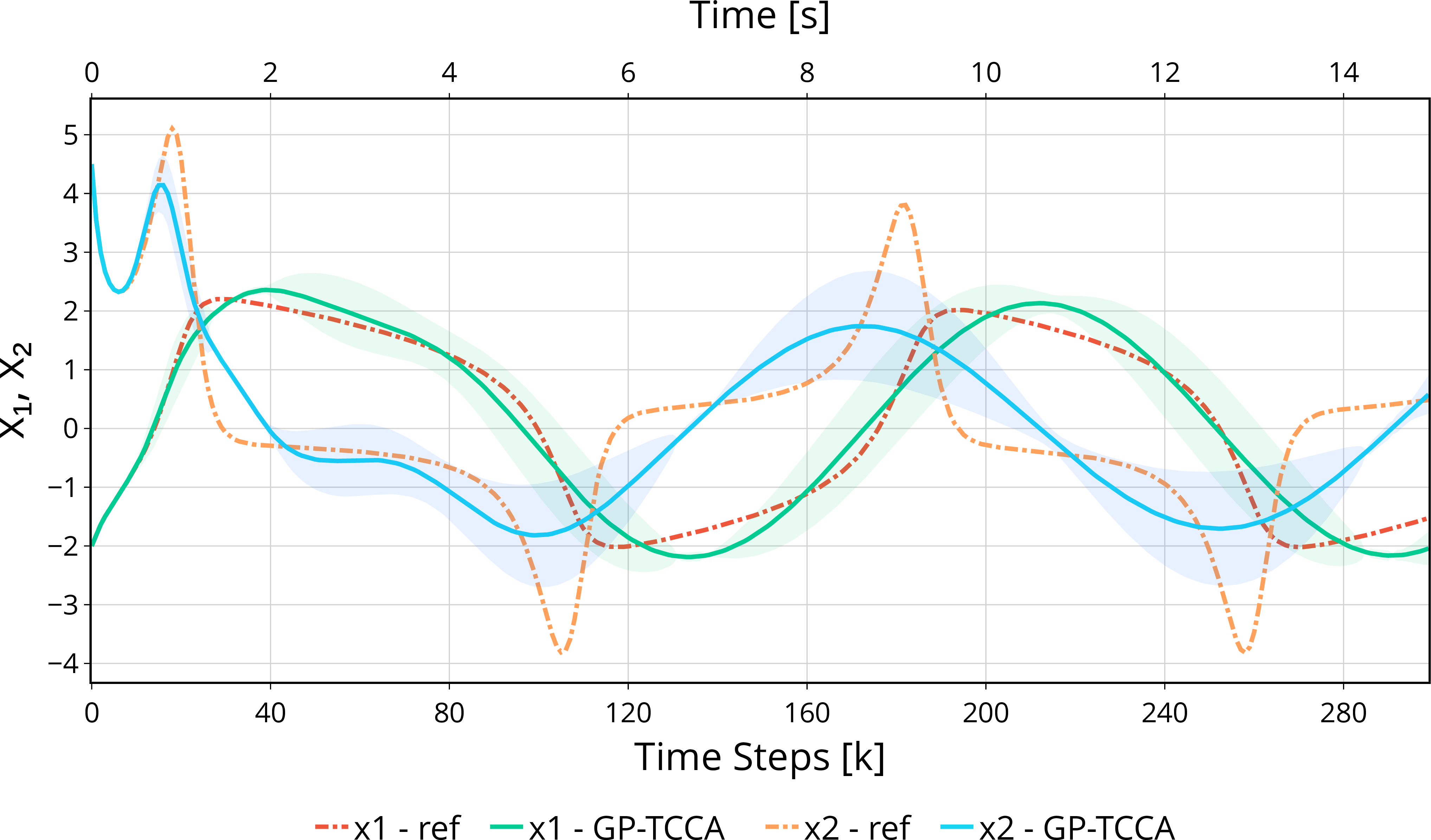
We compared the multi-step errors of our algorithm (referred to as GP-TCCA) using the Van der Pol oscillator as a benchmark: \[\begin{align} {3} \begin{aligned} \dot{x}_{t,1} &= x_{t,2},\\ \dot{x}_{t,2} &= \alpha (1 - x_{t,1}^2) x_{t,2} - x_{t,1}, \end{aligned} \end{align}\] where \(\alpha = 2\) controls the degree of nonlinearity. The dynamical system was simulated by a numerical ODE solver and sampled in time intervals of \(\Delta t = 50.0 \text{ [ms]}\). Figure 1 depicts an example trajectory of the oscillator and its associated forecast.
The metric used to quantify the generalization errors over a test set of \(N_\textrm{tst} = 5000\) noise-free samples was the symmetric mean absolute percentage error (SMAPE; [77]): \[\begin{align} {3} SMAPE = 100\% \frac{3}{N_\textrm{tst}} \sum_{i = 1}^{N_\textrm{tst}} \frac{||\boldsymbol{y}_i - \hat{\boldsymbol{y}}_i||}{||\boldsymbol{y}_i|| + ||\hat{\boldsymbol{y}}_i||}. \end{align}\] The SMAPE equals \(100\%\) if all the model predictions are twice the testing values, i.e., \(\hat{\boldsymbol{y}}_i = 2 \boldsymbol{y}_i\).
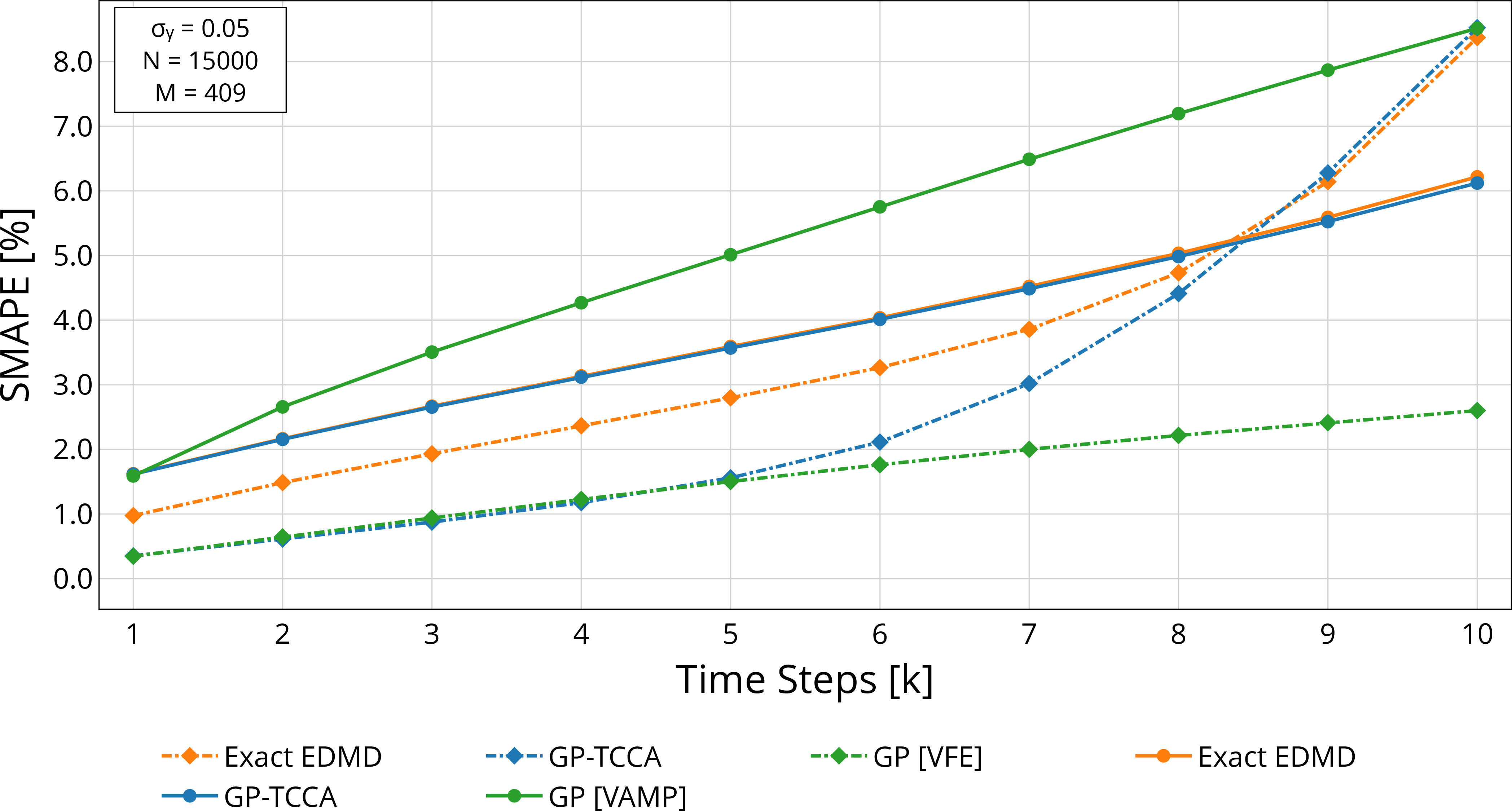
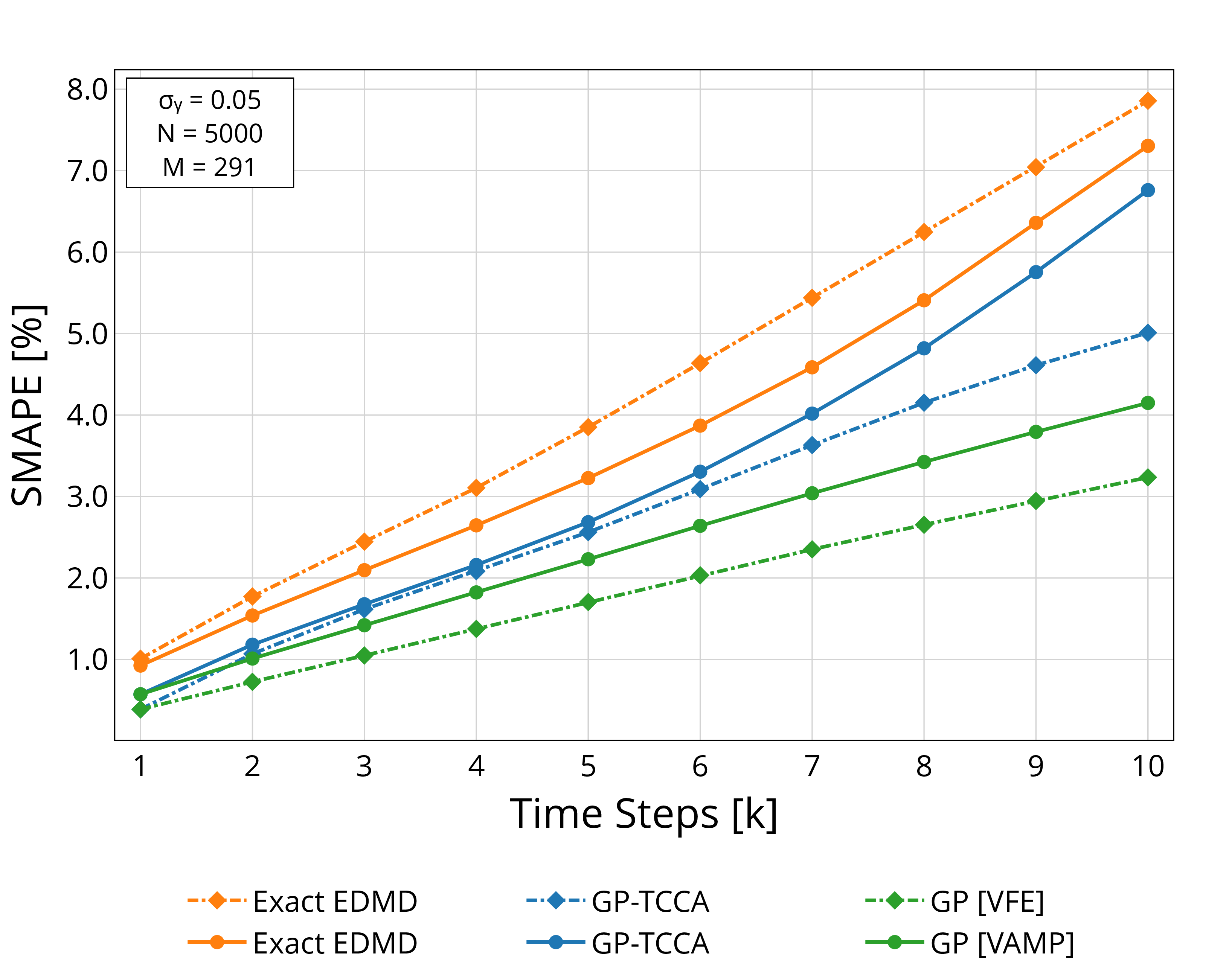
Figure 2: Generalization errors. Comparing SMAPE over multi-step forecasts of GP-TCCA (blue), Exact DMD (orange), and a variational sparse GP (green), with hyperparameters found via VFE (dashed) and VAMP-\(2\) (solid), c.f. Figure 3..
As depicted in Figure 2, alongside our model we implemented two more models and compared their accuracies over multi-step predictions. The first algorithm that we compared ours to is ‘Exact (Extended) DMD’ [78], and the second is a sparse GP model of the flow map [47]. When comparing across the three algorithms, all three models shared the same set of hyperparameters.
We also compared the VFE method to the ‘variational approach to Markov processes’ (VAMP) for hyperparameter optimization [79]. Specifically we maximized the VAMP-\(2\) score of the model.
When optimizing the VAMP score, the two DMD algorithms are virtually indistinguishable, suggesting that the Tikhonov regularization has little to no effect. This indicates that the VAMP-\(2\) objective does not capture sensor noise as effectively as maximizing the VFE of the flow map. Figure 2 shows that our GP-DMD variant outperforms Exact EDMD under noisy conditions. This aligns with our expectations given the explicit treatment of sensor noise and the additional structure imposed by the Bayesian model. However, the nonlinear growth did prompt a closer examination of our regularization strategy.
3.2 Decoupling the Lifted Observation Model↩︎
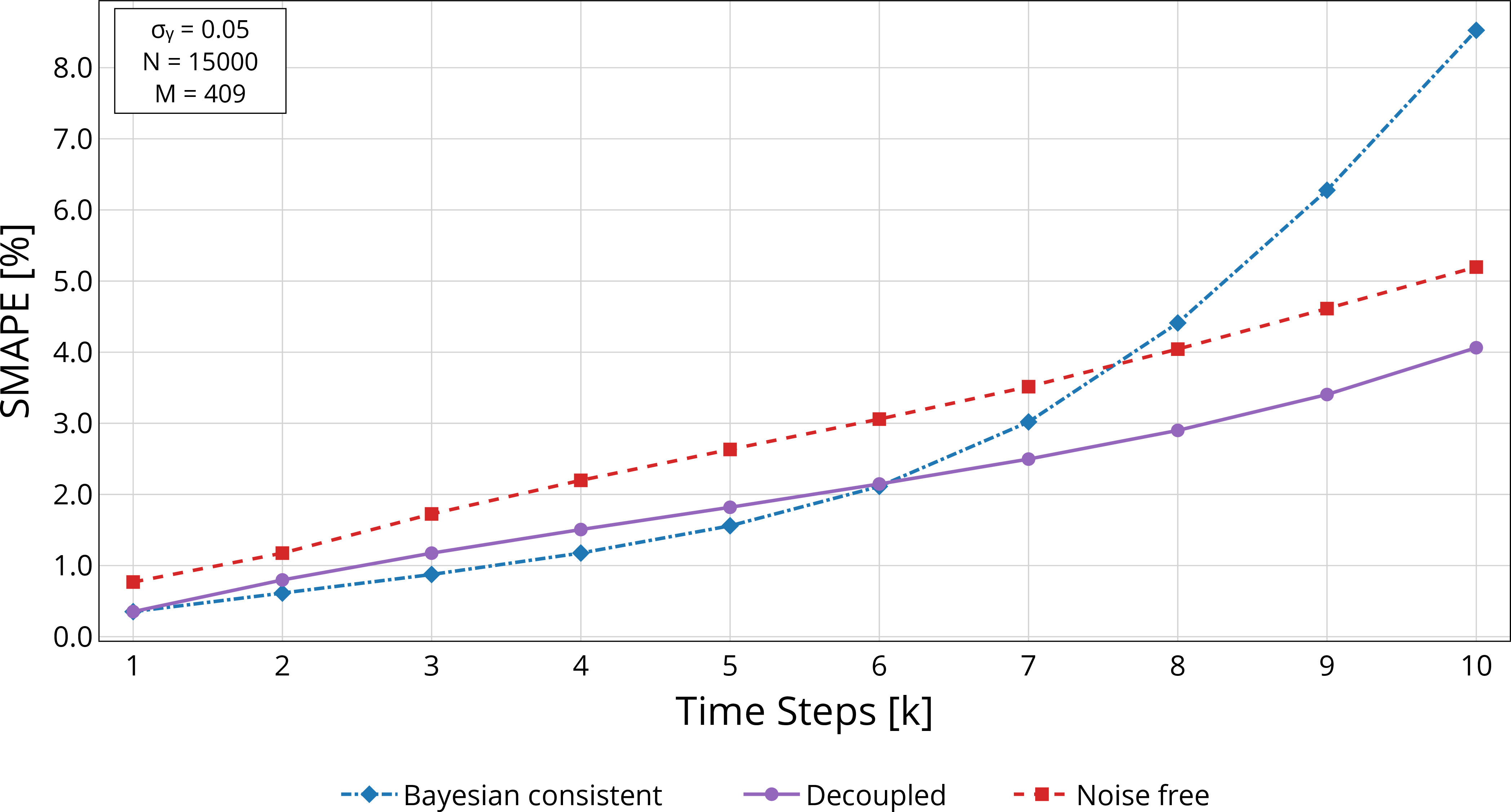
Figure 3: Generalization errors of the decoupled model. Blue: \(\sigma_\mathcal{Y} = \sigma_Y\), purple: \(\sigma_\mathcal{Y} \neq \sigma_Y\), red: \(\sigma_\mathcal{Y} = 0\), c.f. Figure 2..
To assess the sensitivity of our algorithm to the approximation introduced in Definition 1, we separately train a regularization parameter for the lifted model using the kernelized targets \(\mathbf{K}_{ZY}\) (after estimating the optimal kernel hyperparameters and pseudo-inputs as discussed in Section 2.5). In effect, we are defining the RKHS noise model with \(\sigma_\mathcal{Y}^2\kappa_\textrm{bc}\left(\cdot, \cdot\right)\) where \(\sigma_\mathcal{Y}^2\) is not directly coupled to the variance of the sensor noise in the state space, \(\sigma_{Y}^2\). Put differently, the regularization parameter in 4 now corresponds to \(\sigma_\mathcal{Y}\), whereas in 6 it is still \(\sigma_{Y}\). This establishes a division of roles between the two regularization terms: \(\sigma_Y\) is predominantly responsible for projecting to the state space, while \(\sigma_\mathcal{Y}\) controls the accuracies of the multi-step forecasts. Consequently, the relationship in 10 does not hold exactly anymore, but our model is more flexible.
The effect of decoupling is illustrated in Figure 3 where we observe that the growth rate of the GP-TCCA model has markedly reduced, leading to more accurate long-term predictions. We therefore increase the credence in our hypothesis: rigorously accounting for the distortion introduced by the nonlinear feature map will yield a more robust model. For example, we are naturally tempted to model the statistical properties of \(\nu_i\) as non-Gaussian and input-dependent (i.e., heteroskedastic). This is apparent when we notice that \(\kappa_{\mathrm{pr}}(\boldsymbol{x}, Y)\) is typically a nonlinear many-to-one transformation of \(Y\).
3.3 Reprojections↩︎
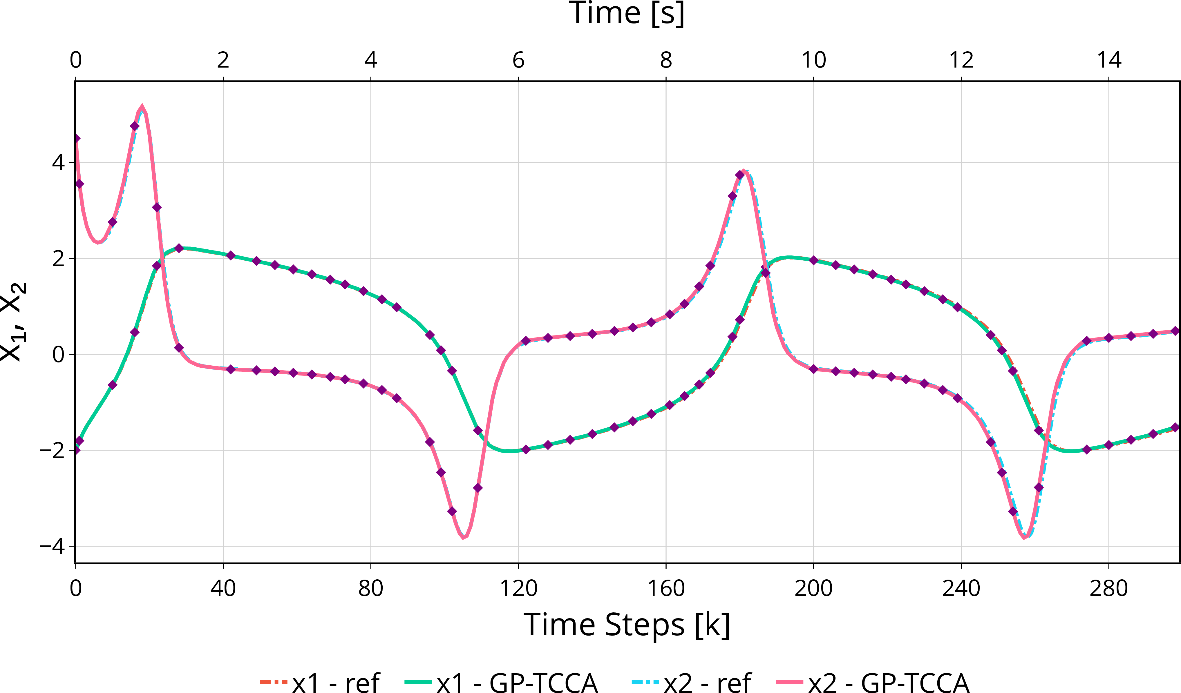
Although the GP model attains the lowest error, the DMD variants are more computationally efficient, because multi-step forecasts follow from spectral propagation (i.e., raising the eigenvalue matrix to the desired power). In contrast, a purely GP-based rollout must repeatedly lift each intermediate state, increasing computational overhead. Consequently, for long horizons, DMD methods often employ a reprojection scheme that combines both approaches; intermittent reprojections onto the state manifold mitigates drift arising from the fact that the learned finite-dimensional subspace may not be perfectly invariant under the true Koopman operator [80].
In Figure 4 we demonstrate how reprojections based on a mechanism defined on 11 can be effectively used to decrease the computational cost while also maintaining accuracy. The idea was simply to reproject when the Euclidean norm of the diagonal entries in \({\mathbf{K}}_{\textrm{pst}}^{k}\left({\boldsymbol{x}}_{0}\right)\) exceeded some predefined tolerance. At such points, the current estimate \(\hat{\boldsymbol{x}}_k\) was treated as a noise-free measurement, and the feature vector \(\mathbf{k}_Z(\hat{\boldsymbol{x}}_k)\) was recomputed5.
For the depicted trajectory, on average a reprojection was performed after every \(5\) time-steps. In other words, the length of the forecasting horizons vary over the state space as the model automatically incorporates its epistemic uncertainty into the predictions. Interestingly, the regions where the vector field changes slowly is where the forecasting horizons are shorter, which suggest that errors accumulate faster in these regions.
3.4 Eigenfunction Uncertainty Quantification↩︎
The second dynamical system that we analyzed was the stochastic well problem described by the overdamped Langevin equation: \[\begin{align} {3} \begin{aligned} \mathrm{d}{x}_{t,1} &= -\nabla_{x_1} V(\boldsymbol{x}_t) \, \mathrm{d}t + \sigma_T \; \mathrm{d}W_{t,1},\\ \mathrm{d}{x}_{t,2} &= -\nabla_{x_2} V(\boldsymbol{x}_t) \, \mathrm{d}t + \sigma_T \; \mathrm{d}W_{t,2},\\ \end{aligned} \end{align}\] where \(W_{t,1}\) and \(W_{t,2}\) are two independent standard Wiener processes. In our experiments, we fixed the noise intensity to \(\sigma_T = 0.7\) and employed a sampling interval of \(\Delta t = 10.0\, [\text{s}]\).



Figure 6: The \(4^\text{th}\) eigenfunction of the stochastic quadruple-well. The coloring depicts a one-standard deviation credible region..
When the potential function is \(V(\boldsymbol{x}_t) = (x_{t,1}^2 - 1)^2 + x_{t,2}^2\), the system has two minima (or “wells"), separated by a barrier, representing the two metastable states of the system. Physically, a particle will spend long periods of time near one of the two minima and only rarely jump over the barrier to the other well due to random thermal fluctuations. By slightly altering the potential function we can increase the number of wells and dominant eigenfunctions. For example, the expression of the potential function for the quadruple-well system is \(V(\boldsymbol{x}_t) = (x_{t,1}^2 - 1)^2 + (x_{t,2} - 1)^2\).
In the context of the double-well problem, the second eigenfunction, depicted in Figure 5, is the first and only non-trivial mode. This eigenfunction captures the switching between the two wells, and reveals the two-state structure and the slow timescale of the transitions [2]. In turn, the quadruple-well has three dominant non-trivial eigenfunctions, one of which we are depicting in Figure 6. Since these systems are reversible, the eigenvalues of the associated PFO and Koopman operators are exclusively real-valued [1].
Figures 5 and 6 show that the well locations align with regions of high certainty. This is because the dynamical systems spend most of their time around the wells, leading to dense sampling in these areas. While the kernel lengthscales also influence the geometry of the low-uncertainty regions, the dominant effect in these plots is the sampling distribution of the training data sets: initial conditions were chosen based on an optimized Latin hypercube design [81], [82], and succeeded by rolling out trajectories with lengths of \(20\) time-steps.
In the bottom plot of Figure 6, propagating the distribution over the eigenfunction forward in time reveals both a mixing and rescaling phenomenon: the eigenfunction collapses while the credible regions around the wells expand, ultimately spanning the entire sampling domain.
4 Conclusion↩︎
We have proposed a sparse kernel-based DMD algorithm which we formulated within a Bayesian framework that treats the embedded Perron–Frobenius operator [39] as a random variable. By unifying operator learning with the mature field of Gaussian process regression the method extends EDMD by incorporating hyperparameter optimization, sparse dictionary learning, enables propagating uncertainties in the eigenfunctions of the flow map, and provides a criteria for reprojections.
The primary insight we have gained from the ablation studies is that kernel transfer operators could benefit from a non-Gaussian and a heteroskedastic observation model; one that is closely intertwined with a Bayesian consistent notion of an operator-valued RKHS. However, we have another reason to modify our model with a more complex noise model; thus far, we have only focused on compensating for measurement noise on the target variables. Yet, DMD is known to be susceptible to adverse effects arising from noise on the inputs [83]–[86]. Incidentally, one approach to dealing with input-noise is a heteroskedastic GP model [62], [87], [88]. Alternatively, in the Koopman community, several variants of DMD have been proposed to correct for the bias induced by input-noise [89]–[92].
Earlier we posed the question of which philosophical stance is most appropriate for kernel transfer operators: a Bayesian or a frequentist perspective. We have argued that the Bayesian viewpoint offers ample opportunities to enrich the interpretation of DMD models. At the same time, we have also demonstrated that diverse perspectives can be especially valuable, as uncovering the reasons for discrepancies between the two paradigms led to the insights that solved the problem. Thus, rather than exclusively favoring one approach above the other, we advocate for employing Bayesian and frequentist methods in tandem whenever possible.
5 Gaussian Process Regression↩︎
Given a training data set \(\mathcal{D} = \{(\boldsymbol{x}_{i}, y_i)\}_{i = 1}^N\) consisting of \(N\) pairs of \(D\)-dimensional inputs (covariates) and scalar outputs (targets or dependent variables), the goal is to estimate the distribution of the function evaluation \(f(\boldsymbol{x}_*)\) at any novel test location \(\boldsymbol{x}_* \in \mathbb{X}\), where \(f \colon \mathbb{X} \rightarrow \mathbb{R}\).
We start by grouping the inputs and outputs into the data matrices \(\mathbf{X}\mathrel{\vcenter{:}}= [\boldsymbol{x}_1,\dots, \boldsymbol{x}_N] \in \mathbb{R}^{D \times N}\) and \(\mathbf{Y}\mathrel{\vcenter{:}}= [y_1, \dots, y_N] \in \mathbb{R}^{1 \times N}\). Note that while GP regression supports a wide variety of input domains, we have defined \(\mathbb{X} \subseteq \mathbb{R}^D\).
Our first modeling assumption is that the sensor noise on the targets is additive, independent, and Gaussian. Consequently, the relationship between the input random variable \(X\) and the output random variable \(Y\) is \[\begin{align} {3} \label{eq:32observation32model} Y_i = f(X_i) + \epsilon_i,\text{where } \epsilon_i \sim \mathcal{N}(0, \sigma_Y^2), \end{align}\tag{12}\] and \(\sigma_Y^2\) is the homoscedastic variance of the sensor noise or the nugget term for surrogate mismodeling [93].
5.1 Reproducing Kernel Hilbert Spaces↩︎
A reproducing kernel \(\kappa: \mathbb{X} \times \mathbb{X} \rightarrow \mathbb{R}\) is a bivariate positive semidefinite function. A rough sketch of the role of a kernel function is as a measure of the similarity (or affinity) between two inputs, \(\boldsymbol{x}\) and \(\boldsymbol{x}'\). This notion of ‘similarity’ is expressed through an inner product between the embeddings of the two inputs into a reproducing kernel Hilbert space (RKHS), \(\mathbb{H}\) [6]. This inner product is embodied by the kernel trick: \[\begin{align} {3} \kappa(\boldsymbol{x}, \boldsymbol{x}') = \langle \kappa(\boldsymbol{x}, \cdot), \kappa(\boldsymbol{x}', \cdot)\rangle_{\mathbb{H}}. \end{align}\]
The kernel trick encapsulates the properties that make RKHS methods so effective. All kernel functions are constructed through the Riesz representation theorem [56], [57], [94], such that the reproducing property \(f(\boldsymbol{x}) = \langle f, \kappa(\boldsymbol{x}, \cdot)\rangle_{\mathbb{H}} \; \forall \; f \in \mathbb{H}\) is satisfied twice over. What this means will become clear shortly. First define the feature map \(\varphi: \mathbb{X} \rightarrow \mathbb{H}\) according to \(\varphi(\boldsymbol{x}) \mathrel{\vcenter{:}}= \kappa(\boldsymbol{x}, \cdot) \in \mathbb{H}\). Now consider that the reproducing property allows us to evaluate any function in \(\mathbb{H}\). What this implies, is that since both \(\varphi(\boldsymbol{x})\) and \(\varphi(\boldsymbol{x}')\) are both elements of \(\mathbb{H}\), they act as the evaluation functionals of the other.
Alternatively, one may think of any two points \(\boldsymbol{x},\boldsymbol{x}' \in \mathbb{X}\) as vertices on a symmetric graph where the weight of the edge connecting them, \(\kappa(\boldsymbol{x}, \boldsymbol{x}')\), is a quantitative comparison between two more complex objects. In this sense, a reproducing kernel defines a local geometry on \(\mathbb{X}\). The practical benefit of the feature map is that while the input data may have very few discernible structures, we can represent more nonlinear structures with \(\varphi(\cdot)\).
5.2 Bayes’ Law↩︎
Informally, Gaussian processes (GPs) are mathematical objects that are generalizations of multivariate normal distributions. Recall that a multivariate normal distribution describes random variables that are vectors of finite dimensionality. If the input domain were real numbers, then roughly speaking the random variable described by a GP is a “vector” of infinite dimensionality indexed not by a natural number but by a real number. More formally, according to the function-space view, a GP represents a probability distribution over \(f \in \mathbb{H}\).
GP regression proceeds following a Bayesian philosophy, which identifies the likelihood with the probability density \(p_\textrm{om}(y_i \mid f, \boldsymbol{x}_i) = \mathcal{N}(y_i; f(\boldsymbol{x}_i), \sigma_Y^2)\). As indicated by the subscript, the likelihood captures the observation model, i.e., the probabilistic mapping between a noise-free latent function evaluation and the noisy target. The likelihood tells us how to update our prior beliefs of the regression function with new data.
It follows that the next step is placing a GP prior over the function \(f(\cdot)\) such that \(p_\textrm{pr}(f) = \mathcal{GP}\left(f; m_\textrm{pr}(\cdot), \kappa_\textrm{pr}(\cdot, \cdot) \right)\). Here \(m_\textrm{pr} : \mathbb{X} \rightarrow \mathbb{R}\) is the prior mean function \(\mathbb{E}[f(\cdot)]\). The second component of the GP prior, the reproducing kernel \(\kappa_\textrm{pr}(\boldsymbol{x}, \boldsymbol{x}')\), encodes \(\mathbb{E}[(f(\boldsymbol{x}) - m_\textrm{pr}(\boldsymbol{x}))(f(\boldsymbol{x}') - m_\textrm{pr}(\boldsymbol{x}'))]\), i.e., the prior covariance between function values.
The combination of the likelihood and the prior defines the generative model. Accordingly, we refer to \(\theta\) as the set of generative hyperparameters, which parameterize both the prior kernel function \(\kappa_\textrm{pr}(\cdot,\cdot)\) and the characteristics of the sensor noise. To lighten the notation, we may omit the dependence of the probability densities on \(\theta\).
An important feature, is that a GP evaluated on the finite subset \(\{\boldsymbol{x}_i\}_{i = 1}^N \subset \mathbb{X}\) is an \(N\)-dimensional multivariate Gaussian random variable. Without loss of generality, if we choose a GP prior with a mean function that is identically zero \(m_\textrm{pr} \equiv 0\), then a priori the function values will behave according to the distribution, \[\begin{align} p_\textrm{pr}(\boldsymbol{f}_X) &= \mathcal{N}^N(\boldsymbol{f}_X ;\boldsymbol{0}, \mathbf{K}_{XX}), \end{align}\] where we have introduced two new variables that are best understood at hand of the dictionary: \[\begin{align} \Phi_X \mathrel{\vcenter{:}}= \begin{bmatrix} \varphi(\boldsymbol{x}_1) & \ldots & \varphi(\boldsymbol{x}_N) \end{bmatrix} \in \mathbb{H}^{1 \times N}. \end{align}\] In essence, the dictionary collects the lifting functions and is a generalization of the design matrix in linear regression.
The adjoint of the dictionary operator is called the observation operator, since \(\Phi_X^\top:\mathbb{H} \rightarrow \mathbb{R}^N\) is a mapping from the feature space to the observable space. By the reproducing property, the observation operator allows us to sample a function \(f \in \mathbb{H}\). Therefore, we can define the vector of latent function values as \(\boldsymbol{f}_X \mathrel{\vcenter{:}}= \Phi_X^\top f =[f(\boldsymbol{x}_1), \ldots, f(\boldsymbol{x}_N)]^\top\), and the variance-covariance matrix by \(\mathbf{K}_{XX} \mathrel{\vcenter{:}}= \big[\kappa_\textrm{pr}(\boldsymbol{x}_i, \boldsymbol{x}_j)\big]_{i,j = 1}^N = \kappa_\textrm{pr}(\mathbf{X}, \mathbf{X}) = \Phi_X^\top \Phi_X\). Simply put, GPs treat every latent function value as a random variable.
The final product of a GP model is the conditional probability density of novel function evaluations [4]. This posterior predictive distribution can be inferred via Bayes’ rule, the prior GP (over both training and test latent values), and the likelihood. Should we assume that the training data set is i.i.d., then the likelihood factorizes over all \(N\) samples, and the exact posterior process over \(f(\cdot)\) can be expressed as \[\begin{align} {3} p_\textrm{pst}(f \mid \mathcal{D}) = \frac{\prod_{i = 1}^N p_\textrm{om}\left(y_i \mid f(\boldsymbol{x}_i \right))p_\textrm{pr}(f) }{\int \prod_{i = 1}^N p_\textrm{om}\left(y_i \mid f(\boldsymbol{x}_i)\right) p_\textrm{pr}(f) \, \mathrm{d}f}. \end{align}\]
Because the likelihood was Gaussian to begin with, the posterior process is also a GP admitting a closed-form expression. To derive this expression, we marginalize out the latent function values at the training points, resulting in a posterior distribution that is fully specified by \[\begin{align} {3} m_\textrm{pst}(\boldsymbol{x}) &\mathrel{\vcenter{:}}= {\mathbf{A}} \, \mathbf{k}_{X}(\boldsymbol{x}) \text{ } , \tag{13}\\ {\kappa}_\textrm{pst}(\boldsymbol{x}, \boldsymbol{x}') &\mathrel{\vcenter{:}}= \kappa_\textrm{pr}(\boldsymbol{x}, \boldsymbol{x}') - \mathbf{k}_{X}^\top(\boldsymbol{x}) \tilde{\mathbf{K}}_{XX}^{-1} \mathbf{k}_{X}(\boldsymbol{x}'), \tag{14} \end{align}\] where \({\mathbf{A}} \mathrel{\vcenter{:}}= \mathbf{Y}\:\tilde{\mathbf{K}}_{XX}^{-1} \in \mathbb{R}^{1 \times N}\) is the weight matrix, \(\tilde{\mathbf{K}}_{XX} \mathrel{\vcenter{:}}= \mathbf{K}_{XX} + \sigma_Y^2 \mathbf{I}_N\) is the covariance matrix for the noisy outputs6, and \(\mathbf{k}_{X}(\boldsymbol{x}) \mathrel{\vcenter{:}}= \Phi_X^\top \varphi(\boldsymbol{x}) = [\kappa_\textrm{pr}(\boldsymbol{x}_1, \boldsymbol{x}), \ldots, \kappa_\textrm{pr}(\boldsymbol{x}_N, \boldsymbol{x})]^\top\) is a feature vector. Now, all our questions about the noisy predictive posterior distribution at some unseen input \(\boldsymbol{x}_*\) can be answered by querying the expression: \[\begin{align} {3} p_\textrm{pst}(y_* \mid \mathcal{D}) = \mathcal{N}(y_*; m_\textrm{pst}(\boldsymbol{x}_*), {\kappa}_\textrm{pst}(\boldsymbol{x}_*, \boldsymbol{x}_*) + \sigma_Y^2). \end{align}\]
Since the quality of the posterior solution is sensitive to \(\theta\), it is typically prudent to first attempt to infer the optimal hyperparameters, \(\theta^*\). The denominator in Bayes’ rule, \(p_\textrm{ml}(\mathbf{Y})\), known as marginal likelihood (or evidence) paves a path to craft an optimization algorithm for model selection, since it takes into account the entire generative model. In other words, it is natural to choose \(\theta^*\), such that it maximizes the probability of observing the targets given the model’s posterior function evaluations. To this end, the closed-form expression for the log-marginal likelihood is \[\begin{align} {3} \operatorname{ln}\left(p_\textrm{ml}\left(\mathbf{Y}\right)\right) &= \operatorname{ln} \left(\int p_\textrm{om}(\mathbf{Y}\mid \boldsymbol{f}_X) p_\textrm{pr}\left(\boldsymbol{f}_X\right) \, \mathrm{d}\boldsymbol{f}_X \right) \label{eq:32exact32evidence}\\ &= -\frac{1}{2} \left[ \underbrace{N \operatorname{ln}(2\pi)}_{\text{constant}} + \underbrace{\operatorname{ln}\left(\left|\tilde{\mathbf{K}}_{XX}\right|\right)}_{\text{model complexity}} + \underbrace{\mathbf{Y}\tilde{\mathbf{K}}_{XX}^{-1} \mathbf{Y}^\top}_{\text{data mismatch}} \right]. \nonumber \end{align}\tag{15}\] Maximizing 15 naturally embodies Occam’s razor, and can be interpreted as engineering the prior GP such that it maximizes the volume of data-matching functions.7
5.3 Sparse Regression↩︎
The most salient downside of GP regression is the computational complexity of identifying the posterior. Computing the exact posterior GP in conventional GP regression requires the inversion of an \(N \!\times\! N\) matrix, which takes \(\mathcal{O}(N^3)\) runtime, and \(\mathcal{O}(N^2)\) memory space to store the weights and the training inputs. The cubic time-complexity and quadratic memory consumption create a bottleneck that hinders GPs from being deployed on data sets larger than a few thousand points.
To mitigate these computational drawbacks, practitioners resort to approximation techniques that employ an additional smaller pseudo-data set. This data set is comprised of pseudo-outputs (i.e., inducing variables) \(\boldsymbol{f}_Z = \Phi_Z^\top f\) that are unknown evaluations of the pseudo-inputs (i.e., inducing inputs or points) \(\mathbf{Z}\mathrel{\vcenter{:}}= \{\boldsymbol{z}_i \in \mathbb{X}\}_{i = 1}^M\). Such pseudo-data set schemes are widely used to reduce a kernel-based algorithm’s training time-complexity to \(\mathcal{O}(N M^2)\) and the memory-complexity to \(\mathcal{O}(NM)\) [96]–[98]. The variable \(M\), representing the cardinality of the pseudo-data set, governs the expressiveness of the sparse GP. The pseudo-inputs, \(\mathbf{Z}\), play a similar role in support or relevance vector machines [9], [99].8
The challenge now becomes to construct an expression for the sparse posterior and jointly infer the hyperparameters and the pseudo-inputs. One approach is to design the approximated posterior GP so that it is as close as possible to the true posterior GP. The phrase “as close as possible" can be, for example, interpreted as minimizing the Kullback–Leibler (KL) divergence between the sparse posterior GP and the exact posterior GP [103]. This particular optimization objective is explored in the variational free energy (VFE) method of [47].
In variational inference of GPs a distribution \(q(f)\) is introduced over the entire infinite-dimensional function \(f\) as an approximation to \(p_\textrm{pst}(f \mid \mathcal{D})\). The primary advantage of the VFE framework is that the pseudo-inputs are treated as variational parameters of an approximated posterior rather than as generative parameters. These variational parameters are automatically protected from overfitting, since the optimization is between the exact posterior and an approximated posterior. In other words, the variational parameters are resilient against assumptions about the generative model[87]. Another advantage of the VFE method is that increasing \(M\) is guaranteed to monotonically improve the approximation.
Definition 2. The variational free energy (VFE; [104]): \[\begin{align} {3} \mathcal{F}(\theta, \mathbf{Z}) \mathrel{\vcenter{:}}= \int \operatorname{ln}\left(\frac{p(\mathbf{Y}, f \mid \theta)}{q(f)}\right) q(f) \, \mathrm{d}f \leq \operatorname{ln}(p_\textrm{ml}(\mathbf{Y})), \end{align}\] is often referred to as the evidence lower bound (ELBO).
Under the i.i.d. data assumption, the VFE can be written as \[\begin{align} {3} \mathcal{F}(\theta, \mathbf{Z}) &= \sum_{i = 1}^N \int \text{ ln}(p_\textrm{om}(y_i \mid f_{i}, \theta)) q(f_{i} \mid \theta) \, \mathrm{d}f_i \\&- KL\left(q(\boldsymbol{f}_Z) \,||\, p_\textrm{pr}(\boldsymbol{f}_Z \mid \theta)\right), \end{align}\] where \(q(\boldsymbol{f}_Z)\) is a free-form multivariate Gaussian distribution, and \(p_\textrm{pr}(\boldsymbol{f}_Z \mid \theta) = \mathcal{N}^M(\boldsymbol{f}_Z; \boldsymbol{0}, \mathbf{K}_{ZZ})\) refers to the prior Gaussian distribution over the pseudo-outputs \(\boldsymbol{f}_Z\).
Due to the Gaussian assumptions, the calculus of variations can be used to analytically solve for the optimal approximate posterior Gaussian process. This results in the following posterior mean and covariance functions: \[\begin{align} {3} m_\textrm{pst}(\boldsymbol{x}) &\mathrel{\vcenter{:}}= {\mathbf{A}} \: \mathbf{k}_{Z}(\boldsymbol{x}), \tag{16}\\ {\kappa}_\textrm{pst}(\boldsymbol{x}, \boldsymbol{x}') &\mathrel{\vcenter{:}}= \kappa_\textrm{pr}(\boldsymbol{x}, \boldsymbol{x}') - \mathbf{k}_{Z}^\top(\boldsymbol{x}) \text{ }\tilde{\mathbf{B}}\text{ }\mathbf{k}_{Z}(\boldsymbol{x}'). \tag{17} \end{align}\] Here, we are deviating from the notation in [47] to highlight the similarities with (kernel) ridge-regression. The weight matrix, \({\mathbf{A}} \! \mathrel{\vcenter{:}}= \! \mathbf{Y}\, \mathbf{K}_{ZX}^\top \, \tilde{\mathbf{C}}_{XX}^{-1}\), contains the regression coefficients obtained from linear operations on matrices. The noisy Gramian is defined by \(\tilde{\mathbf{C}}_{XX} \! \mathrel{\vcenter{:}}= \! \mathbf{K}_{ZX}\mathbf{K}_{ZX}^{\top} \! + \! \sigma_Y^2\mathbf{K}_{ZZ}\), and the cross-covariance matrix by \(\mathbf{K}_{ZX} \! \mathrel{\vcenter{:}}= \! \kappa_\textrm{pr}(\mathbf{Z}, \mathbf{X}) \! \in \! \mathbb{R}^{M\times N}\). Lastly, to compute the posterior kernel the weights for the information gain term are \(\tilde{\mathbf{B}} \! \mathrel{\vcenter{:}}= \! \left(\mathbf{K}_{ZZ}^{-1} -\sigma_Y^2 \! \tilde{\mathbf{C}}_{XX}^{-1}\right)\).
The VFE, i.e., the quantity that we maximize, is \[\begin{align} {3} \label{eq:32VFE} &\mathcal{F}(\theta, \mathbf{Z}) = \operatorname{ln}\left( \mathcal{N}^N(\mathbf{Y}; \boldsymbol{0}, \tilde{\mathbf{R}})\right) - \frac{1}{2\sigma_Y^2} \operatorname{Tr}\left(\mathbf{K}_{XX} - \mathbf{R}\right), \end{align}\tag{18}\] where \(\mathbf{R} \mathrel{\vcenter{:}}= \mathbf{K}_{ZX}^\top\mathbf{K}_{ZZ}^{-1}\mathbf{K}_{ZX}\) is the Nyström approximation to the exact prior covariance matrix, and \(\tilde{\mathbf{R}} \mathrel{\vcenter{:}}= \mathbf{R} + \sigma_Y^2\mathbf{I}_N\) is its noisy variant [105]. Notice that the closed-form expression in 18 is very similar to that of the exact log-marginal likelihood 15 , with the addition of the trace term. The trace term encourages pseudo-inputs to better capture the training data, and is proportional to the sum of the variances of the training function values given the pseudo-targets, \(p\left(\boldsymbol{f}_X \mid \boldsymbol{f}_Z\right)\), i.e., the total squared error of predicting \(\boldsymbol{f}_X\) given \(\boldsymbol{f}_Z\).
6 Transfer Operator Theory↩︎
GP regression as presented in Appendix 5 can directly be applied to time-series data. However, if we merge GP regression with transfer operator theory we can efficiently perform multi-step predictions and, as advertised earlier, gain a deeper understanding of the dynamical system.
To that end, we proceed by recalling the definition of the Koopman operator for random dynamical systems (RDSs), specifically for stationary and ergodic Markov processes [2], vcrnjaric2020koopman?. These include, for example, stochastic differential equations driven by Gaussian white noise and discrete systems generated by i.i.d. random maps.
Consider the continuous-time stochastic dynamical systems represented by the time-homogeneous Itô stochastic differential equation (SDE), \[\begin{align} {3} \label{eq:32Ito} \mathrm{d}\boldsymbol{x}_t = \mathbf{r}(\boldsymbol{x}_t) \, \mathrm{d}t + \mathbf{h}(\boldsymbol{x}_t) \, \mathrm{d}W_t, \quad t \geq 0, \end{align}\tag{19}\] where \(\{ \boldsymbol{x}_t \}_{t \geq 0}\) is a stochastic process defined on the state space \(\mathbb{X}\), and \(W_t\) is the \(D\)-dimensional standard Wiener process (i.e., Brownian motion). Such stochastic dynamics arise when there is process noise present in the system, which enters in the form of a diffusion term \(\mathbf{h}(\boldsymbol{x}_t)\). The first term \(\mathbf{r}(\boldsymbol{x}_t)\), is commonly referred to as the friction or drift term. Both \(\mathbf{h} \colon \mathbb{X} \to \mathbb{X}\) and \(\mathbf{r} \colon \mathbb{X} \to \mathbb{X}\) are assumed to be smooth time-invariant nonlinear vector fields.
While Koopman theory covers continuous-time dynamics, we convert to discrete-time dynamics by sampling trajectories at uniform time intervals, \(\Delta t\), such that \(t_k \mathrel{\vcenter{:}}= \Delta t \, k\), which implies \(t_k + \Delta t = t_{k + 1}, \text{ } \forall \text{ } k\in \mathbb{N}\). The resulting discrete-time Markov process can be represented by the flow map \(\boldsymbol{F}_\alpha \colon \mathbb{X} \to \mathbb{X}\), which is indexed by the random variable \(\alpha \in \Omega\) such that \(Y = \boldsymbol{F}_\alpha(X)\), where \(\Omega\) is the probability space associated with the stochastic dynamics. The resulting discrete-time RDS, possesses a transition density function, \(p_{\Delta t}: \mathbb{X} \times \mathbb{X} \rightarrow \mathbb{R}_{\geq 0}\), such that the expression \(p_{\Delta t}(\boldsymbol{x}_{k+1} \mid \boldsymbol{x}_k)\) represents the conditional probability of observing the next state \(\boldsymbol{x}_{k + 1}\) given the current state \(\boldsymbol{x}_k\).
6.1 The Koopman and Perron–Frobenius Operators↩︎
The starting point for Koopman theory is mapping the RDS from the lower-dimensional nonlinear space \(\mathbb{X}\) to a higher-dimensional linear space \(\mathbb{G}\), such that no information is lost when moving to this feature space. In short, operator theory can be viewed as a trade-off between lifting the state space into a feature space with more complex states but simpler dynamics. To perform the lifting, the literature defines an observable function as, \(g \in \mathbb{G}\), where \(\mathbb{G} = \mathcal{L}^\infty(\mathbb{X})\).9
Definition 3. The stochastic Koopman operator (SKO) [26], [106] \(\mathcal{U} \colon \mathbb{G} \rightarrow \mathbb{G}\) is defined as the conditional expectation of any observable composed with the flow, \[\begin{align} {3} (\mathcal{U}g)(\boldsymbol{x}) &= \mathbb{E}\left[g(Y) \mid X = \boldsymbol{x}\right]\\ &=\int p_{\Delta t}(\boldsymbol{y} \mid \boldsymbol{x}) \, g(\boldsymbol{y}) \, \mathrm{d}\boldsymbol{y}. \end{align}\]
In general, an observable may be a vector-valued function, \(\mathbf{g} \in \mathbb{G}^P\). Of particular interest is the full-state observable, \(\mathbf{g}(\boldsymbol{x}) = \boldsymbol{x}\), and the extended-state observable, \(\mathbf{g}(\boldsymbol{x}) = \mathbf{k}_{X}(\boldsymbol{x})\). From a theoretical perspective, we often only consider scalar-valued observables, \(g \colon \mathbb{X} \to \mathbb{R}\), and have \(\mathcal{U}\) act component-wise on the set of observables \(\{ g_i\}_{i=1}^P\).
Definition 4. The Perron–Frobenius operator (PFO) is concerned with an ensemble of trajectories and acts on the conjugate space of probability densities \(\mathcal{P}: \mathcal{L}^1(\mathbb{X}) \rightarrow \mathcal{L}^1(\mathbb{X})\): \[\begin{align} {3} (\mathcal{P}p) (\boldsymbol{y}) &=\int p_{\Delta t}(\boldsymbol{y} \mid \boldsymbol{x}) \, p(\boldsymbol{x}) \, \mathrm{d}\boldsymbol{x}. \end{align}\]
Hence we call any operator, transporting some object (a distribution, or an observable) by the dynamics, a transfer operator, i.e., the action of the process on functions of the state. The mathematical formulations of kernel transfer operators follow from the assumptions that the observables are elements of an RKHS feature space, and the operators are compact with a discrete spectrum [39]. This implies that we may set \(\mathbb{G} = \mathbb{H}\).
Strictly speaking, the definitions of kernel transfer operators are formulated in the language of kernel mean embeddings (KMEs) [107]. KME is another statistical learning theory, which typically falls within the frequentist paradigm. KME is closely associated with kernel principal component analysis (KPCA) and kernel canonical correlation analysis (KCCA), both of which are considered to be unsupervised learning techniques [100], [108]–[112]. For the sake of completeness, the theory describing KMEs is recapitulated in Appendix 7.
6.2 Koopman Mode Decomposition↩︎
The crux of transfer operator analysis rests upon the fact that the nonlinear dynamics are linear in the eigenfunction coordinates [1]. These eigenfunctions \(\{ \phi_i \in \mathbb{G}\}_{i = 1}^\infty\), and the corresponding eigenvalues \(\{ \lambda_i \in \mathbb{C}\}_{i = 1}^\infty\), of \(\mathcal{U}\), obey the following equation in discrete time: \[\begin{align} {3}\label{eq:koopman32eigen} \phi_i(\boldsymbol{x}_{k+1}) = \mathcal{U} \phi_i(\boldsymbol{x}_k) = \lambda_i \phi_i(\boldsymbol{x}_k). \end{align}\tag{20}\] Assuming that the dynamical systems we are dealing with have discrete point spectra, the evolution of the observables can be expanded in terms of the eigenfunctions and the eigenvalues. Specifically we can write the infinite series: \[\begin{align} {3} (\mathcal{U}\mathbf{g})(\boldsymbol{x}) = \sum_{i = 1}^\infty \mathbf{v}_i \lambda_i \phi_i(\boldsymbol{x}), \end{align}\] which is a generalization of the Sturm–Liouville expansion for a differential problem.
Every Koopman mode, \(\mathbf{v}_i \in \mathbb{C}^P\), is determined by the dictionary of observables and is associated with an eigenpair \((\lambda_i, \phi_i)\). The modes are in essence the coefficients used to construct \(\mathbf{g}(\cdot)\) using the Koopman eigenfunction basis. In other words, the observables can be expanded into a weighted sum of eigenfunctions: \[\mathbf{g} = \sum_{i = 1}^\infty \mathbf{v}_i \phi_i \in \mathbb{G}^P.\]
Altogether, the modes and eigenpairs allow us to reconstruct and propagate the system’s state arbitrarily far into the future [26]. Where the eigenvalues describe the temporal behavior of the dynamical system, the modes capture the spatial behavior. Once we have found the sequence of triplets \(\{(\lambda_i, \phi_i, \mathbf{v}_i)\}_{i = 1}^\infty\) for a dynamical system, we have completed its Koopman mode decomposition (KMD; [106], [113]).
6.3 Finite-Dimensional Approximation↩︎
The challenge is that the Koopman operator is infinite-dimensional. As far as numerical methods are concerned, we want to find a reduced but finite set \(\{(\lambda_i, \phi_i, \mathbf{v}_i)\}_{i = 1}^M\), such that the evolution of all observable functions can be reasonably well approximated. That is, the goal is to derive a matrix representation of the SKO by projecting it onto a finite-dimensional subspace, such that a finite-dimensional linear system is induced [28].
The matrix representation of the transfer operator can be obtained by restricting the operator to an invariant subspace. Note that when the Koopman operator of a dynamical system has a continuous eigenvalue spectrum, as is the case for chaotic systems, the discretization will be flawed [114], [115].
The subspace spanned by the elements of \(\Phi_Z\), \(\mathbb{G}_M \mathrel{\vcenter{:}}= \text{span}\{ \Phi_Z\}\), is invariant if all observables \(g \in \mathbb{G}_M\) can be written as a linear combination of the dictionary functions, \[\begin{align} {3} g = \sum_{i = 1}^M q_{i} \; \varphi(\boldsymbol{z}_i) = \Phi_Z \boldsymbol{q}, \quad \boldsymbol{q} \in \mathbb{R}^M, \end{align}\] and they remain in this subspace after acted upon by the Koopman operator, i.e., \(\mathcal{U}g \in \mathbb{G}_M\) [26].
On route to a finite-dimensional matrix representation, we define a bounded linear map \(\Gamma_Z \colon \mathbb{G} \to \mathbb{R}^M\) that yields the coordinates of an observable in the basis \(\{ \varphi(\boldsymbol{z}_i)\}_{i=1}^M\). Applying \(\Gamma_Z\) to an observable \(g \in \mathbb{G}\) returns the coefficients, \(\boldsymbol{q} = \Gamma_Z \; g \in \mathbb{R}^M\). In turn, having the dictionary operator act on \(\boldsymbol{q}\), will recover the best approximation to the observable in \(\mathbb{G}_M\), \(\Phi_Z \boldsymbol{q} = \Pi_Z g \approx g\), where \(\Pi_Z \mathrel{\vcenter{:}}= \Phi_Z \, \Gamma_Z\). For an invariant subspace, it is evident that \(\Pi_Z\) commutes with \(\mathcal{U}\), which implies that \(\Gamma_Z \, \Phi_Z = \mathbf{I}_M\), and hence \(\mathbb{G} = \mathbb{G}_M\).
Altogether the compression of the Koopman operator to the subspace \(\mathcal{U}_M : \mathbb{G} \rightarrow \mathbb{G}_M\) is \[\begin{align} {3} \mathcal{U}_M \mathrel{\vcenter{:}}= \Pi_Z \, \mathcal{U} = \Phi_Z \, \Gamma_Z \, \mathcal{U}. \end{align}\] From here we can define the finite-dimensional matrix representation \(\mathbf{U}: \mathbb{R}^M \rightarrow \mathbb{R}^M\) of \(\mathcal{U}\) s.t. \[\begin{align} {3} \mathcal{U}_M \, g = \Pi_Z \, \mathcal{U} \, \Pi_Z \, g= \Phi_Z \, \mathbf{U}\, \Gamma_Z \, g, \quad g \in \mathbb{G}, \end{align}\] which defines the Koopman matrix as \[\begin{align} {3} \label{eq:32koopman32matrix} \mathbf{U}\mathrel{\vcenter{:}}= \Gamma_Z \, \mathcal{U} \, \Phi_Z \in \mathbb{R}^{M \times M}. \end{align}\tag{21}\]
Several well-known results relate the spectral properties of the Koopman matrix \(\mathbf{U}\) to those of the operator \(\mathcal{U}\). For example, we can decompose the eigenfunctions \(\{ \phi_i\}_{i = 1}^M\) with \[\begin{align} {3} \phi_i = \sum_{j =1}^M \mathrm{w}_{ij} \, \varphi(\boldsymbol{z}_j) = \Phi_Z \,\boldsymbol{\mathrm{w}}_i, \quad \boldsymbol{\mathrm{w}}_i \in \mathbb{C}^M, \end{align}\] and then apply the relationship between eigenvalues and eigenfunctions 20 : \[\begin{align} {3} \mathcal{U}_M \phi_i &= \lambda_i \phi_i, \\ \Phi_Z \mathbf{U}\Gamma_Z \phi_i &= \lambda_i \Phi_Z \Gamma_Z \phi_i, \\ \mathbf{U}\Gamma_Z \phi_i &= \lambda_i \Gamma_Z \phi_i, \\ \mathbf{U}\boldsymbol{\mathrm{w}}_i &= \lambda_i \boldsymbol{\mathrm{w}}_i. \end{align}\] Hence, the right eigenvectors of \(\mathbf{U}\) correspond to the coordinates of the eigenfunctions in the basis of dictionary functions, and the eigenvalues of \(\mathbf{U}\) are the eigenvalues of \(\mathcal{U}\). The left eigenvectors of \(\mathbf{U}\) are the modes of the extended-state observable, and are related to the eigenfunctionals of the dual operator to the Koopman operator [1].
7 Embedding Probability Distributions↩︎
Unlike GP regression, which treats parameters as random variables, the kernel mean embedding (KME) approach relies on repeated sampling from a population to inform on estimates of probability distributions, and treats regression as a purely geometric operation between vector spaces. This geometric view is a reformulation of the frequentist least-squares solution rather than an entirely separate paradigm.
From the outset, KME allows for featurization of the output variable, while GP regression is typically presented with pure scalar-valued outputs10. In other words, the output space \(\mathbb{Y}\) is not limited to \(\mathbb{Y} \subseteq \mathbb{R}\) [116]. In contrast with 13 we directly model \(\mathbb{E}_{Y \mid \boldsymbol{x}}[g(Y) \mid X = \boldsymbol{x}], \; g \in \mathbb{H}_Y\). Apart from this, the mathematical formalisms for the predictive mean 13 and the kernel conditional mean embedding 23 are exactly the same, as are the predictive variance 14 and the Mahalanobis distance [117], [118]. It is a case where the GP regression and KME communities, have developed overlapping tools while having different goals in mind.
A limitation of the KME approach is that it recovers only part of the structure available in GP regression: in particular, other concepts such as the marginal likelihood do not translate directly into the embedding framework.
7.1 Marginal Distributions↩︎
The idea of KMEs are to identify probability distributions with elements of an RKHS that fully capture their statistical features. Operationally, we map the data to an RKHS and then we compute the mean. The embeddings are not direct estimates of probability distributions, but rather representative points or elements in an RKHS. For readers interested in embedding probability distributions in RKHSs, excellent resources are [107], [116], [119].
Definition 5. Marginal Mean Embedding. Let \(\mathbb{H}_X\) be an RKHS with a bounded kernel11. Then the kernel mean embedding \(\mu_X \in \mathbb{H}_X\) is defined as \[\begin{align} {3} \mu_X \mathrel{\vcenter{:}}= \mathbb{E}_X\left[\varphi(X)\right] = \int_{\mathbb{X}}^{} \varphi(\boldsymbol{x}) \, \mathrm{d}\mathbb{P}_{X}(\boldsymbol{x}), \end{align}\] where the integral is a Bochner integral [56], [121].
For a large class of kernel functions known as characteristic kernels [122], [123], the mean embedding captures all the necessary information about the distribution \(\mathbb{P}_{X}\). In other words, the mean map \(\mathbb{P}_{X} \rightarrow \mu_X\) is injective and there is no information lost when mapping the distribution into \(\mathbb{H}_X\).
By virtue of the reproducing property and linearity of expectation, the marginal embedding \(\mu_X\) has the property that the expectation of any Hilbert space function \(f\in \mathbb{H}_X\) can be evaluated as an inner product, i.e., \(\mathbb{E}_X \left[f(X)\right]= \langle f,\mu_X \rangle_{\mathbb{H}_X}\).
To realize an unbiased consistent empirical estimate \(\hat{\mu}_X\) of \(\mu_X\) we require that the sample set be drawn independently and identically distributed (i.i.d.) from \(\mathbb{P}_{X}\). The estimate of the mean embedding can then be calculated with \[\begin{align} {3} \hat{\mu}_X \mathrel{\vcenter{:}}= \frac{1}{N} \sum\limits_{i = 1}^N \kappa(\boldsymbol{x}_i, \cdot). \end{align}\]
7.2 Joint Distributions↩︎
The next step is to generalize to two (or more) random variables. For joint probability distributions we compute covariance operators over tensor product spaces of RKHSs [124].
Definition 6. Joint Mean Embedding. Let \((Y, X)\) be a joint random variable on \(\mathbb{Y}\times \mathbb{X}\) with the joint distribution \(\mathbb{P}_{YX}\). Given the characteristic kernels \(\kappa_X\) and \(\kappa_Y\) with respective RKHSs \(\mathbb{H}_X\) and \(\mathbb{H}_Y\), where each kernel is parametrized by \(\theta_X\) and \(\theta_Y\), and the associated feature maps are \(\varphi_X\) and \(\varphi_Y\). The trace-class variance-covariance operator \(\mathcal{C}_{XX}:\mathbb{H}_X \rightarrow \mathbb{H}_X\) and Hilbert–Schmidt cross-covariance operator \(\mathcal{C}_{YX} : \mathbb{H}_X \rightarrow \mathbb{H}_Y\) are defined as \[\begin{align} {3} \begin{aligned} \mathcal{C}_{YX} &\mathrel{\vcenter{:}}= \mathbb{E}_{YX}\left[\varphi_{YX}(Y,X)\right] = \int_{\mathbb{X} \times \mathbb{Y}}^{} \varphi_{YX}(\boldsymbol{y},\boldsymbol{x}) \, \mathrm{d}\mathbb{P}_{YX}(\boldsymbol{y},\boldsymbol{x}), \\ \mathcal{C}_{XX} &\mathrel{\vcenter{:}}= \mathbb{E}_X\left[\varphi_{X}(X,X)\right] = \int_{\mathbb{X}}^{} \varphi_{XX}(\boldsymbol{x},\boldsymbol{x}) \, \mathrm{d}\mathbb{P}_{X}(\boldsymbol{x}), \end{aligned} \end{align}\] where the joint feature map is defined according to \(\varphi_{YX}(\boldsymbol{y}, \boldsymbol{x}) \mathrel{\vcenter{:}}= \varphi_Y(\boldsymbol{y}) \otimes \varphi_X(\boldsymbol{x})\). Through the joint feature map, a pair of realizations \((\boldsymbol{y},\boldsymbol{x})\) can be lifted into the tensor-product feature space \(\mathbb{H}_{YX} \mathrel{\vcenter{:}}= \mathbb{H}_Y \otimes \mathbb{H}_X\), i.e., the space of linear operators from \(\mathbb{H}_Y\) to \(\mathbb{H}_X\).
The cross-covariance operator expresses the covariance between functions in \(\mathbb{H}_{YX}\), and contains all the information regarding the dependencies of \(X\) and \(Y\). If both \(\kappa_X\) and \(\kappa_Y\) are linear kernels such that the feature maps \(\varphi_X\) and \(\varphi_Y\) are identity maps, we recover the standard covariance matrices. Hence, one may think of \(\mathcal{C}_{XX}\) and \(\mathcal{C}_{YX}\) as nonlinear generalizations of these matrices. Using these ideas, the cross-covariance between two functions \(f \in \mathbb{H}_X\) and \(g \in \mathbb{H}_Y\) is \[\begin{align} {3} \mathbb{E}_{YX} \left[f(X) g(Y) \right] &= \langle f, \mathcal{C}_{XY} g \rangle_{\mathbb{H}_X} = \langle \mathcal{C}_{YX} f, g \rangle_{\mathbb{H}_Y}\\ &=\langle g \otimes f, \mathcal{C}_{YX} \rangle_{\mathbb{H}_{YX}}. \end{align}\]
Therefore, \(\mathcal{C}_{XX}\) is a self-adjoint operator and \(\mathcal{C}_{YX}\) is the adjoint of \(\mathcal{C}_{XY}\). Note that the joint feature map is a rank one operator. Consequently, there is an interesting duality of perspectives at play, because just like the mean embedding was an element in the RKHS \(\mu_X \in \mathbb{H}_X\), so the cross-covariance operator is an element in the tensor product feature space \(\mathcal{C}_{YX} \in \mathbb{H}_{YX}\).
The empirical estimators for the covariance operators given i.i.d. samples \(\{ (\boldsymbol{x}_i,\boldsymbol{y}_i) \}_{i = 1}^N\) are: \[\begin{align} {3} \label{eq:32estimate32covariance32operators} \begin{aligned} \hat{\mathcal{C}}_{YX} &\mathrel{\vcenter{:}}= \frac{1}{N}\sum\limits_{i = 1}^N \varphi_{YX}(\boldsymbol{y}_i, \boldsymbol{x}_i) = \frac{1}{N}\Phi_Y\Phi_X^\top,\\ \hat{\mathcal{C}}_{XX} &\mathrel{\vcenter{:}}= \frac{1}{N}\Phi_X\Phi_X^\top, \; \text{and} \; \hat{\mathcal{C}}_{YY} \mathrel{\vcenter{:}}= \frac{1}{N}\Phi_Y\Phi_Y^\top. \end{aligned} \end{align}\tag{22}\]
7.3 Conditional Distributions↩︎
We are now in a position to introduce RKHS embeddings of conditional probability distributions, known as conditional mean embeddings (CMEs). To do so, we require the following result, which relates the two operators \(\mathcal{C}_{XX}\) and \(\mathcal{C}_{XY}\).
Proposition 1. If \(\, \mathbb{E}_{Y \mid X}\left[g(Y) \! \mid X = \! \cdot \right] \! \in \! \mathbb{H}_X \; \forall \; g \in \mathbb{H}_Y\), then \(\mathcal{C}_{XX} \mathbb{E}_{Y \mid X} \left[g(Y) \mid X \! = \! \cdot \right] = \mathcal{C}_{XY}g\), see [122].
Definition 7. Conditional Mean Embedding [116].Assuming that Proposition 1 holds, then the CME of \(\mathbb{P}_{(Y \mid X=\cdot)}\) is the operator \(\mathcal{C}_{Y \mid X} : \mathbb{H}_X \rightarrow \mathbb{H}_Y\), whereas the evaluation of the conditional distribution \(\mathbb{P}_{Y \mid \boldsymbol{x}}\) corresponds to the element \(\mu_{Y \mid \boldsymbol{x}} \in \mathbb{H}_Y\): \[\begin{align} {3} \begin{aligned} \mathcal{C}_{Y \mid X} &\mathrel{\vcenter{:}}= \mathcal{C}_{YX} \mathcal{C}_{XX}^{-1}, \\ \mu_{Y \mid \boldsymbol{x}} &\mathrel{\vcenter{:}}= \mathcal{C}_{Y \mid X} \text{ }\varphi_X(\boldsymbol{x}). \end{aligned} \end{align}\]
From the reproducing property it follows that \[\begin{align} {3} \begin{aligned} \mathbb{E}_{Y \mid \boldsymbol{x}}\left[g(Y) \mid X = \boldsymbol{x}\right] &= \langle \mathcal{C}_{XX}^{-1} \mathcal{C}_{XY} g, \varphi_X(\boldsymbol{x}) \rangle_{\mathbb{H}_X}\\ &= \langle g, \mu_{Y \mid \boldsymbol{x}} \rangle_{\mathbb{H}_Y} \; \forall \; g \in \mathbb{H}_Y \label{eq:32CME32eval}. \end{aligned} \end{align}\tag{23}\]
The condition \(\mathbb{E}_{Y \mid X}\left[g(Y) \mid X = \cdot \right] \in \mathbb{H}_X \; \forall \; g \in \mathbb{H}_Y\), will always hold for finite domains with characteristic kernels, but may not be valid for a continuous domain [125]. A common approach to extend the condition to other systems is to consider the regularized inverse \((\mathcal{C}_{XX} + \varepsilon \mathcal{I})^{-1}\), where \(\mathcal{I}\) is the identity operator on \(\mathbb{H}_X\), and \(\varepsilon > 0\) is a Tikhonov regularization parameter [126]. Moreover, \(\mathcal{C}_{XX}\) is a compact trace class operator, with eigenvalues that accumulate at zero when \(\mathbb{H}_X\) is infinite dimensional [56]. The regularization ensures a well-posed inverse.
All that is missing from the framework are the estimators for the CME. The empirical estimator of \(\mathcal{C}_{Y \mid X}\) is given by, \[\begin{align} {3} \hat{\mathcal{C}}_{Y \mid X} &= \hat{\mathcal{C}}_{YX}(\hat{\mathcal{C}}_{XX} + \varepsilon \mathcal{I})^{-1} \\ &= \frac{1}{N} \Phi_Y \Phi_X^\top \left(\frac{1}{N}\Phi_X \Phi_X^\top + \varepsilon \mathcal{I} \right)^{-1}\\ &= \Phi_Y \left(\mathbf{K}_{XX} + N\varepsilon \mathbf{I}_N \right)^{-1} \Phi_X^\top\\ &= \Phi_Y \tilde{\mathbf{K}}_{XX}^{-1} \Phi_X^\top. \end{align}\] Note that we can rescale the Tikhonov parameter \(\varepsilon \mathrel{\vcenter{:}}= \sigma_{Y}^2/N\), to coincide with the Bayesian interpretation and notation used in Appendix 5.
The empirical estimator of \({\mu}_{Y \mid \boldsymbol{x}}\) permits the intuitive description as a weighted sum of dictionary elements \(\Phi_Y\), where the weights are dependent on the data point in \(\mathbb{X}\) on which we are conditioning. This line of reasoning leads us to \[\begin{align} {3} \hat{\mu}_{Y \mid \boldsymbol{x}} \mathrel{\vcenter{:}}= \sum\limits_{i = 1}^{N} \varphi_Y(\boldsymbol{y}_i) \alpha_i(\boldsymbol{x}) = \Phi_Y \; \boldsymbol{\alpha}(\boldsymbol{x}), \end{align}\] where the weight vector is \[\begin{align} {3} \boldsymbol{\alpha}(\boldsymbol{x}) \mathrel{\vcenter{:}}= \tilde{\mathbf{K}}_{XX}^{-1} \; \mathbf{k}_{X}(\boldsymbol{x}) \in \mathbb{R}^N. \end{align}\] Now the resemblance between 23 and 13 should be apparent. Moreover, it is easy to see that the CME coincides with the expression for the embedded PFO found in 2 when the input and output feature spaces are equal, i.e., \(\mathbb{H}_X = \mathbb{H}_Y\).
8 Estimation Algorithm↩︎
Here we detail a time-lagged canonical correlation analysis (TCCA) algorithm to yield a GP-DMD model. The algorithm is a variant of the algorithm in [79], [111], to which interested readers are referred for a more thorough theoretical discussion.
TCCA is a multivariate statistical method applicable to two sets of ‘featurized’ variables that are related by the flow map of a dynamical process. The algorithm is especially attractive, because it performs a decomposition that is similar to DMD, but with a valid interpretation for both reversible and irreversible processes, and for stationary and non-stationary processes. It finds a pair of linear orthonormal transformations – one for each set – such that the resulting projections are maximally correlated in time. The Koopman matrix can then be expressed in terms of these two transformations.
2
Using the transformation \(\boldsymbol{\Psi}_Z(\cdot) \mathrel{\vcenter{:}}= \mathbf{L}_{ZZ}^{-1} \, \mathbf{k}_Z(\cdot)\) start by preconditioning the cross-covariance matrices: \[\begin{align} {3} \mathbf{\Psi}_{ZX} &\mathrel{\vcenter{:}}= \mathbf{L}^{-1}_{ZZ} \mathbf{K}_{ZX}, \\ \mathbf{\Psi}_{ZY} &\mathrel{\vcenter{:}}= \mathbf{L}^{-1}_{ZZ} \mathbf{K}_{ZY}. \end{align}\] The lower triangular matrix \(\mathbf{L}_{ZZ}\) is obtained from the Cholesky decomposition of \(\mathbf{K}_{ZZ} + \sigma_Z^2\mathbf{I}_M\). This step simplifies upcoming computations, because the regularized Gramian matrix factorizes according to \[\begin{align} {3} \tilde{\mathbf{C}}_{XX} = \mathbf{L}_{ZZ} \, \left(\mathbf{\Psi}_{ZX} \mathbf{\Psi}_{ZX}^\top + \sigma_{Y}^2\mathbf{I}\right) \, \mathbf{L}_{ZZ}^\top. \end{align}\]
In this basis construct the \(M \times M\) Gramian and stiffness matrices: \[\begin{align} {3} \mathbf{G}_{XX} &\mathrel{\vcenter{:}}= \mathbf{\Psi}_{ZX} \, \mathbf{\Psi}_{ZX}^\top,\\ \mathbf{G}_{YY} &\mathrel{\vcenter{:}}= \mathbf{\Psi}_{ZY} \, \mathbf{\Psi}_{ZY}^\top,\\ \mathbf{G}_{XY} &\mathrel{\vcenter{:}}= \mathbf{\Psi}_{ZX} \, \mathbf{\Psi}_{ZY}^\top. \end{align}\]
Proceed by performing (truncated) singular value decompositions (SVD) on the preconditioned covariance matrices: \[\begin{align} {3} \mathbf{\Psi}_{ZX} &\approx \mathbf{M}_X \mathbf{\Sigma}_X \mathbf{H}_{X}^\top,\\ \mathbf{\Psi}_{ZY} &\approx \mathbf{M}_Y \mathbf{\Sigma}_Y \mathbf{H}_{Y}^\top. \end{align}\]
Now we can include regularization by simply adding the noise variances to each of the principal variances: \[\begin{align} {3} \mathbf{\tilde{\Sigma}}_{X,i} &= \sqrt{\mathbf{\Sigma}_{X,i}^2 + \sigma_{Y}^2}. \end{align}\] This implies that the inverse and inverse square root of the (noisy) Gramian matrices can be expressed as \[\begin{align} {3} \tilde{\mathbf{G}}_{XX}^{-1} &= \mathbf{M}_X \mathbf{\tilde{\Sigma}}_{X}^{-2} \mathbf{M}_X^\top, \\ {\mathbf{G}}_{YY}^{-1/2} &= \mathbf{M}_Y \mathbf{{\Sigma}}_{Y}^{-1} \mathbf{M}_Y^\top. \end{align}\]
After normalizing the preconditioned cross-covariance matrices with \(\tilde{\mathbf{G}}_{XX}^{-1/2}\) and \(\tilde{\mathbf{G}}_{YY}^{-1/2}\), the half-whitened Koopman matrix can be computed with \[\begin{align} {3} \mathbf{U}' &= \tilde{\mathbf{G}}_{XX}^{-1/2} \, \mathbf{G}_{XY} \, \tilde{\mathbf{G}}_{YY}^{-1/2}, \end{align}\] which has the SVD: \[\begin{align} {3} \mathbf{U}' &\approx \mathbf{W}_X' \,\mathbf{P} \, \mathbf{W}_Y'^\top. \end{align}\]
Compute the transformation matrices: \[\begin{align} {3} \mathbf{W}_X = {\tilde{\mathbf{G}}}_{XX}^{-1/2} \mathbf{W}_X', \: \mathbf{W}_Y = \tilde{\mathbf{G}}_{YY}^{-1/2} \mathbf{W}_Y'. \end{align}\]
Since the Markov model decomposes according to \[\begin{align} {3} \mathbb{E} \left[ \mathbf{W}_Y^\top \boldsymbol{\Psi}_Z(Y) \right] &= \mathbf{P} \, \mathbb{E} \left[ \mathbf{W}_X^\top \boldsymbol{\Psi}_Z(X) \right], \\ \mathbb{E} \left[ \boldsymbol{\Psi}_Z(Y) \right] &= \left( \mathbf{W}_X \mathbf{P} \mathbf{W}_Y^{-1} \right)^\top \mathbb{E} \left[ \boldsymbol{\Psi}_Z(X) \right] \\ &= \mathbf{U}^\top \mathbb{E} \left[ \boldsymbol{\Psi}_Z(X) \right], \end{align}\] the final Koopman matrix in the preconditioned basis is \[\begin{align} {3} \mathbf{U}&= \mathbf{W}_X \,\mathbf{P} \, \mathbf{W}_Y^\top \, \tilde{\mathbf{G}}_{YY}. \end{align}\]
The eigenvalue decomposition of \(\mathbf{U}\) will return \({\mathbf{V}}_{\kappa}\), and the modes with respect to the full-state observable are \[\begin{align} {3} {\mathbf{V}}_{f} &= \mathbf{\Lambda}^{-1} \, {\mathbf{V}}_{\kappa} \, \tilde{\mathbf{G}}_{XX}^{-1} \, \mathbf{\Psi}_{ZX} \mathbf{Y}^\top. \end{align}\]
8.1 Further Remarks↩︎
Cholesky preconditioning. Similar to [40], the Cholesky preconditioning step was also quite beneficial for numerical stability. As a bonus, due to the lower triangular structure of \(\mathbf{L}_{ZZ}\) the preconditioned matrices are efficiently found by solving the systems of linear equations.
Jitter term and noisy pseudo–outputs. The jitter term, \(\sigma_Z^2\), may be regarded as another variational hyperparameter that we can optimize, and implies that the pseudo-outputs \(\boldsymbol{f}_Z\) are noisy.
TCCA interpretation and Koopman singular functions. As mentioned, TCCA provides another set of quantities by which we can analyze and interpret the dynamical system. The left and right singular functions of the Koopman operator are respectively approximated by \(\mathbf{W}_X^\top \boldsymbol{\Psi}_Z(\cdot)\) and \(\mathbf{W}_Y^\top \boldsymbol{\Psi}_Z(\cdot)\), and can be used to identify coherent sets [127], [128].
The goal of TCCA is to simultaneously transform \(\mathbf{\Psi}_Z(X)\) and \(\mathbf{\Psi}_Z(Y)\) in such a way that the cross-correlation between the whitened vectors are diagonal. More formally, the first canonical correlation is defined by the optimization problem in primal form: \[\begin{align} {3} \rho_1 &= \max_{\mathbf{w}_X,\,\mathbf{w}_Y} \frac{\operatorname{cov}\left(\mathbf{w}_X^\top \mathbf{\Psi}_Z(X),\,\mathbf{w}_Y^\top \mathbf{\Psi}_Z(Y) \right)}{\sqrt{\operatorname{var} \left( \mathbf{w}_X^\top \mathbf{\Psi}_Z(X))\,\operatorname{var}(\mathbf{w}_Y^\top \mathbf{\Psi}_Z(Y) \right)}} \\ &= \max_{\mathbf{w}_X,\,\mathbf{w}_Y} \operatorname{corr} \left( \mathbf{w}_X^\top \mathbf{\Psi}_Z(X),\,\mathbf{w}_Y^\top \mathbf{\Psi}_Z(Y) \right), \end{align}\] subject to constraining the images to unit variance \[\begin{align} {3} \operatorname{var}\left( \mathbf{w}_X^\top \mathbf{\Psi}_Z(X)\right) = 1 &\approx (1/N) \, \mathbf{w}_X^\top \tilde{\mathbf{G}}_{XX} \mathbf{w}_X, \\ \operatorname{var}\left( \mathbf{w}_Y^\top \mathbf{\Psi}_Z(Y)\right) = 1 &\approx (1/N) \, \mathbf{w}_Y^\top \tilde{\mathbf{G}}_{YY} \mathbf{w}_Y. \end{align}\] The problem is then generalized to finding an ordered list of correlations, which we package into the diagonal matrix \(\mathbf{P}\), along with the associated transformations \(\mathbf{W}_X\) and \(\mathbf{W}_Y\).
Hyperparameter selection via VAMP score. As we demonstrated in Section 3, choosing the hyperparameters can be accomplished with a VAMP-score, which is a metric that quantifies the similarity between the estimated singular functions and the true ones. An example is the squared sum of canonical correlations, i.e., the VAMP-\(2\) score or the total kinetic variance [129], which is a quantity that reaches its maximum when all the patterns extracted from the data are perfectly linear, i.e., \(\rho_i = 1 \, \forall \,i \, \in \left[ \textrm{min}(\textrm{dim}(\mathbf{\Sigma}_X), \textrm{dim}(\mathbf{\Sigma}_Y)) \right]\).
9 The Bayesian-consistency kernel↩︎
Since \(\nu_i\) is an \(\mathbb{H}\)-valued Gaussian random element defined by the covariance operator \(\mathcal{C}_{\mathrm{bc}}\), i.e., \[\begin{align} {3} \mathbb{E}\big[\langle \nu_i, \, g \rangle_{\mathbb{H}}\,\langle \nu_i, \, f \, \rangle_{\mathbb{H}}\big] =\langle g, \,\mathcal{C}_{\mathrm{bc}} \, f \rangle_{\mathbb{H}} \quad \forall\, f,g\in\mathbb{H}. \end{align}\] Then the induced scalar process \(\nu_i(\boldsymbol{x}) = \langle \nu_i,\varphi(\boldsymbol{x})\rangle_{\mathbb{H}}\) is a Gaussian process associated with the Bayesian-consistency kernel, and can be related to the feature map of the prior covariance function: \[\begin{align} {3} \kappa_\mathrm{bc}(\boldsymbol{x}, \, \boldsymbol{x}') = \langle \varphi(\boldsymbol{x}), \, \mathcal{C}_{\mathrm{bc}} \, \varphi(\boldsymbol{x}') \rangle_{\mathbb{H}}. \end{align}\] Since \(\mathbf{K}_{\mathrm{bc}} \mathrel{\vcenter{:}}= [\kappa_{\mathrm{bc}}(\boldsymbol{z}_i, \boldsymbol{z}_j)]_{i,j = 1}^M \in \mathbb{R}^{M \times M}\) it follows that \[\begin{align} {3} \mathbf{K}_{\mathrm{bc}} = \Phi_Z^{\top} \, \mathcal{C}_{\mathrm{bc}} \, \Phi_Z. \end{align}\] Given a finite-rank approximation of \(\mathcal{C}_{\mathrm{bc}}\) supported on the span of \(\Phi_Z\), such that \[\begin{align} {3} \mathcal{C}_{\mathrm{bc}} \approx \sum_{i, j = 1}^M \mathbf{C}_{\mathrm{bc}, \, ij} \; \varphi(\boldsymbol{z}_i) \otimes \varphi(\boldsymbol{z}_j) = \Phi_Z \, \mathbf{C}_{\mathrm{bc}} \, \Phi_Z^\top, \quad \mathbf{C}_{\mathrm{bc}} \in \mathbb{R}^{M \times M}, \end{align}\] we obtain the expression \[\begin{align} {3} \mathbf{C}_{\mathrm{bc}} = \mathbf{K}_{ZZ}^{-1} \, \mathbf{K}_{\mathrm{bc}} \, \mathbf{K}_{ZZ}^{-1}. \end{align}\]
References↩︎
The superscript attached to \(\mathcal{GP}\) indicates the dimensionality of the random object associated with the Gaussian process.↩︎
The unscented transform is also an alternative and very attractive approach [67].↩︎
For stationary kernels the quadratic form of 8 enables an approximation of \(\nabla^2(\boldsymbol{x})\) that requires only gradient information [68].↩︎
One could consider including other Subset of Data algorithms, e.g. [74], [75].↩︎
In evaluating \({\mathbf{\Xi}}_{\textrm{pst}}^{1}(\boldsymbol{x}) = {\kappa}_\textrm{pst}(\boldsymbol{x}, \boldsymbol{x}) \, \mathbf{K}_\textrm{bc}\) and subsequently 8 , we employed spectral propagation with \({\mathbf{V}}_{\kappa}\) to compute the feature vector \(\mathbf{k}_Z(\hat{\boldsymbol{x}}_k)\), thereby bypassing multiple evaluations of a potentially costly kernel function.↩︎
The noise kernel models a constant covariance over the state space \(\mathbb{X}\) with \(\kappa_\sigma(\boldsymbol{x},\boldsymbol{x}') \mathrel{\vcenter{:}}= \sigma^2\delta(\boldsymbol{x},\boldsymbol{x}')\), which is a scaled Kronecker delta function. Couple this with the fact that the sum of kernel functions is a valid kernel.↩︎
One can often find an analytical expression for the gradient of 15 and use optimization algorithms such as conjugate gradient ascent or BFGS [95].↩︎
Speed-ups can also be realized through low-rank methods, such as partial Gram–Schmidt orthogonalization [5], [100], random Fourier features [101], [102], or the LASSO-like algorithm of [61].↩︎
Other Banach spaces for \(\mathbb{G}\) are also valid, e.g., the Hilbert space of Lebesgue square-integrable functions, i.e., \(\mathbb{G} \mathrel{\vcenter{:}}= L^2(\mathbb{X})\) [39], ikeda2022koopman?.↩︎
In this work, we bridge the gap by providing a Bayesian interpretation of \(\varphi(Y)\).↩︎
Stationary kernels (functions only depending on the distance between the inputs), such as the Matérn or squared exponential kernels, are bounded \(\text{sup}_{\boldsymbol{x}, \boldsymbol{y} \in \mathbb{X}} \kappa(\boldsymbol{x},\boldsymbol{y}) < \infty\) [4], [120].↩︎