Sufficient conditions for strong discrete maximum principles in finite element solutions of linear and semilinear elliptic equations
August 31, 2025
Abstract
We introduce a novel technique for proving global strong discrete maximum principles for finite element discretizations of linear and semilinear elliptic equations for cases when the common, matrix-based sufficient conditions are not satisfied. The basic argument consists of extending the strong form of discrete maximum principle from macroelements to the entire domain via a connectivity argument. The method is applied to discretizations of elliptic equations with certain pathological meshes, and to semilinear elliptic equations.
1 Introduction↩︎
The preservation of qualitative properties constitutes a central theme in the design of numerical methods for partial differential equations. Among those properties, maximum principles have captured the attention of many generations of numerical analysts, as they play an essential role in ensuring that solutions maintain their physical relevance. For example, it is not only desired, but sometimes critical that quantities representing concentrations lie in the interval [0,1], that computed densities are positive, or that fluxes across interfaces have the correct sign.
In this work we focus on discrete maximum principles (DMPs) for finite element solutions of linear and semilinear elliptic equations. A short and particular formulation of the DMP is that the maximum of a discrete subharmonic function cannot be achieved in the interior of its domain unless the function is constant. At the discrete level we distinguish between the local DMP, which refers to the DMP being satisfied on the union of elements with a common vertex, and the global DMP, which refers to the entire domain; verifying the latter is the ultimate goal, but also presents a greater challenge. A long list of works [1]–[13] (to cite only a few) was devoted to studying conditions under which appropriate forms of the global DMP hold for linear and nonlinear elliptic equations. Many more references can be found in the review article [14] and the recent monograph [15]. A common element for all these articles is the hypothesis that certain key matrices have nonpositive off-diagonal elements; for the case of the linear Poisson equation, this reduces to the necessity for the stiffness matrix to be an \(M\)-matrix (see [16] for definition). Not only is this condition restrictive on the mesh (see Definition 2.2 in [14]), but it is equivalent to the local DMP to be satisfied around each vertex. Hence, it is fair to say that most of the aforementioned works use various techniques to globalize the DMP, after essentially assuming the local DMP holds everywhere. However, in [17] (Section 6) it is shown that the global DMP can hold on certain meshes where local DMPs do not hold. Therefore, the nonpositivity of the off-diagonal entries is not a necessary condition for the global DMP (see also [15], Example 6.10, p. 159).
Moreover, an example is given [17] where the global DMP fails, even as the mesh size converges to zero. It is notable how challenging it is to find an example where the finite element spaces have good approximation properties, but the global DMP fails; in fact the global DMP seems to hold for many practical situations. Hence, it is fair to say that there is a gap in the literature between the known sufficient and the necessary conditions for the global DMP to hold. In this paper we are providing a set of conditions that aim to bridge this gap. We also note that approximation alone allows proving a weaker form of the DMP [18], [19].
The main contribution in this article is to provide a novel technique for proving a global strong DMP (sDMP) for several classes of elliptic equations. The main ingredient consists of extending the sDMPs from macroelements to the entire domain using a connectivity argument; nonpositivity of the off-diagonal entries of the stiffness matrix is not assumed to hold everywhere. The general theorems are applied to linear elliptic equations that include “defects” (edges that lead to positive off-diagonal entries in the stiffness matrix), degenerate meshes, as well as semi-linear elliptic equations.
This paper is organized as follows. After introducing the maximum principles in Section 2, we present the main results in abstract form in Section 3. These are applied to linear elliptic equations in Section 4, where we also connect the new technique with classical results. In Section 5 we apply our framework to problems with mesh defects, and in Section 6 we prove the sDMP for a class of semilinear elliptic equations; the latter results may not be completely new, but they further showcase the wide scope of our method’s applicability. Some conclusions are formulated in Section 7.
2 Motivation and problem formulation↩︎
In this section we introduce the model problems of interest and the classical maximum principles, on which we model their discrete counterparts in Section 3.
2.1 The continuous model problems and their maximum principles↩︎
Let \(D\subset \mathbb{R}^d\) (\(d=2, 3\)) be a polygonal or polyhedral domain, and consider the monotone semilinear elliptic boundary value problem \[\begin{equation} \tag{1} -\sum_{i,j=1}^d \partial_i(a_{ij}(x)\partial_j u(x)) + c(x,u(x)) = f(x)\;\;\mathrm{in} \;\; D, \end{equation} \begin{equation} \tag{2} u|_{\partial D} = g, \end{equation}\] with \(a_{ij}=a_{ji}\in C^{0,1}(\overline{D})\) for \(1\le i, j \le d\), and \[\begin{align} \label{eq:ellop} \underline{a}|v|^2\le \sum_{i,j=1}^d a_{ij}(x) v_i v_j \le \overline{a}|v|^2,\;\;\forall v\in \mathbb{R}^d \end{align}\tag{3}\] for some constants \(0<\underline{a}\le \overline{a}\). Assume the reaction term \(c:D\times \mathbb{R}\to \mathbb{R}\) satisfies the following conditions: \[\begin{align} \tag{4} &\forall x\in D,\; c(x,0)=0, \;\;\mathrm{and}\;\;c(x,\cdot)\;\;\mathrm{is\; nondecreasing;}\\ &\tag{5} {\color{black}c(\cdot,0)\in L^{\frac{p}{2}}(D)\;\mathrm{for\;some\;}p>d;}\\ &\tag{6} \exists L_c>0, \;\;\forall x\in D,\; \forall u, v\in \mathbb{R},\;|c(x,u)-c(x,v)| \le L_c |u-v|. \end{align}\] This includes the linear case when \[\begin{align} \label{eq:Creaclinear} &c(x,u) = \tilde{c}(x)\: u \end{align}\tag{7}\] for some nonnegative function \(\tilde{c}\in L^{\infty}(D)\). For existence, uniqueness, and regularity results for 1 2 see [20] and the references therein.
For a function \(u\) we define \(u^+ = \max (u,0)\), and \(u^- = -\min(u,0)\). Note that \(u^+,u^-\ge 0\) and \(u=u^+-u^-\). The continuous problem 1 2 is known [21], [22] to satisfy the following strong maximum principles:
Theorem 1. Assume \(c\equiv 0\) in 1 , \(a_{ij}\) are continuously differentiable, and \(u\in C^2(D) \cap
C^1(\overline{D})\) solves 1 2 .
(i) If \(f\ge 0\), then \[\label{eq:linmaxprincpos}
\min_{\overline{D}}u \ge \min_{\partial D} u.\tag{8}\] In addition, if \(u\) attains a minimum over \(\overline{D}\) at \(x_0\in D\) (i.e., an
interior point), then \(u\) is constant.
(ii) If \(f\le 0\), then \[\label{eq:linmaxprincneg}
\max_{\overline{D}}u \le \max_{\partial D} u.\tag{9}\] In addition, if \(u\) attains a maximum over \(\overline{D}\) at \(x_0\in D\) (i.e., an
interior point), then \(u\) is constant.
Theorem 2. Assume \(c\) is given by 7 , with \(c\) and \(a_{ij}\) being continuously differentiable, and \(u\in C^2(D) \cap C^1(\overline{D})\) solves 1 2 .
(i) If \(f\ge 0\), then \[\label{eq:slmaxprincpos}
\min_{\overline{D}}u \ge -\max_{\partial D} u^-.\tag{10}\] In addition, if \(u\) attains a nonpositive minimum over \(\overline{D}\) at \(x_0\in
D\) (i.e., an interior point), then \(u\) is constant.
(ii) If \(f\le 0\), then \[\label{eq:slmaxprincneg}
\max_{\overline{D}}u \le \max_{\partial D} u^+.\tag{11}\] In addition, if \(u\) attains a nonnegative maximum over \(\overline{D}\) at \(x_0\in
D\) (i.e., an interior point), then \(u\) is constant.
In this work we analyze a set of conditions under which maximum principles similar to Theorems 1-2 hold for finite element discretizations of 1 2 . In light of this goal, we note that for the continuous problem the strong maximum principle holds on any sufficiently regular subdomain \(E\subseteq D\); for the discretized problem such maximum principles may hold on the full domain, but not on subdomains, and vice versa.
We also remark that the maximum principles for the continuous problem are used in this work only to serve as models for their discrete counterparts; the continuous problem and its properties does not play any role in the analysis of the discrete maximum principle that we present in the next sections.
2.2 Finite element discretization↩︎
The weak form of 1 2 reads: given \(u^b\in H^1(D)\) so that \(u^b|_{\partial D}=g\) and \(f\in H^{-1}(D)\), find \(u\in H^1(D)\) so that \(u^0=u-u^b\in H_0^1(D)\) satisfies \[\begin{align} \label{eq:weakellcont} a_D(u^0+u^b,v) + \left( c(\cdot, u^0+u^b) , v \right)_{D} =\left< f , v \right>_D,\;\;\forall v\in H_0^1(D)\;, \end{align}\tag{12}\] where \(\left< \cdot , \cdot \right>_D\) is dual pairing, \(\left( \cdot , \cdot \right)_D\) is the \(L^2\)-inner product on \(D\), and \[\begin{align} \label{eq:bilform} a_D(u,v)=\sum_{i,j=1}^d \int_D a_{ij}\:\partial_i u \:\partial_j v,\;\;\forall u, v\in H^1(D). \end{align}\tag{13}\] Let \({\mathcal{T}}_h\) be a triangulation of \(\overline{D}\) with vertices \((P_i)_{1\le i\le N}\), and consider the space \(V^h(\overline{D})\) of continuous piecewise linear functions with respect to \({\mathcal{T}}_h\), and \(V_0^h(\overline{D})=\{\varphi\in V^h(\overline{D})\;: \varphi|_{\partial D} = 0\}\). Let \((\varphi_i)_{1\le i\le N}\) the associated standard nodal basis in \(V^h(\overline{D})\) (including boundary nodes). Denote by \({\mathcal{I}}_h:C(\overline{D})\to V_h(\overline{D})\) be the nodal interpolation operator defined by \[\begin{align} {\mathcal{I}}_h u = \sum_{i=1}^N u(P_i) \varphi_i. \end{align}\] The finite element solution of 1 2 on \(D\) reads: find \(u_h\in V^h(\overline{D})\) of the form \(u_h = u_h^0+ u_h^b\) with \(u_h^0\in V_0^h(\overline{D})\), and \(u_h^b = {\mathcal{I}}_h u^b\), so that \[\begin{align} \label{eq:weakelldisc} a_D(u_h^0+u_h^b,v) + \left( c(\cdot,u_h^0+u_h^b) , v \right)_D=\left< f , v \right>_D,\;\;\forall v\in V_0^h(\overline{D}). \end{align}\tag{14}\] A set \(E \subseteq D\) is called a discrete subdomain (of \(D\)) if \(E\) is a union of simplices of \({\mathcal{T}}_h\). When solving the problem on a discrete subdomain \(E\), then \(E\) must replace \(D\) everywhere in 14 . Due to the potential nonlinearity of the reaction term \(c\) in the second argument, the term \(\left( c(\cdot, u_h^0+u_h^b) , v \right)_D\) is replaced with a cubature, preferably one that involves only function values at the vertices. This is equivalent to interpolating the aforementioned term prior to integration. More precisely, 14 can be solved in practice using the following formulation: \[\begin{align} \label{eq:weakelldiscinterp} a_D(u_h^0+u_h^b,v) + \left( {\mathcal{I}}_h c(\cdot,u_h^0+u_h^b) , v \right)_D=\left< f , v \right>_D,\;\;\forall v\in V_0^h(\overline{D}). \end{align}\tag{15}\] The formulations 14 and 15 are certainly equivalent if \(c(x,u)=\tilde{c} u\) with \(\tilde{c}\ge 0\) constant, but in general they are not. Cf. [23], both the continuous variational problem 12 as well as its discrete version 14 are well-posed. In preparation for the results in Section 3, we highlight the following localization property of the finite element solutions:
Lemma 1. Let \(E\subseteq D\) be a discrete subdomain of \(D\). If \(u^D_h\) is the solution of 14 or 15 on \({D}\) and \(u^E_h\) solves 14 or 15 , respectively, on \({E}\) with boundary condition \(u^E_h|_{\partial E} = u^D_h|_{\partial E}\), then \(u^E_h = u^D_h|_{E}\).
Proof. The argument is the same for both formulations, so we focus on the former. First note that \(u^D_h|_E\) satisfies the required boundary condition on \(E\) (in a trivial manner). Consider the subset of nodal basis functions supported in \(\overline{E}\), that is, \(N_E = \{i\: :\: \mathrm{supp}(\varphi_i)\subseteq \overline{E}\}\). Since 14 holds for all \(v=\varphi_i\) with \(i\in N_E\), all the integrals in 14 are, in effect, restricted to \(E\). Also note that \(V_0^h(\overline{E})\) is generated by the set \(\{\varphi_i|_E\: :\: i\in N_E\}\). Hence, \(u^D_h|_E\) satisfies 14 with the set \(E\) replacing \(D\). ◻
Essentially, Lemma 1 states that the restriction of a finite element solution to a discrete subdomain \(E\) is a finite element solution on \(E\) with appropriate boundary conditions.
3 Abstract strong discrete maximum principles↩︎
3.1 Abstract solution operators↩︎
Denote \(V^h(\partial D) = \{\varphi|_{\partial D}\: :\: \varphi\in V^h(\overline{D})\}\). We say that \(f\in (V_0^h(\overline{D}))^*\) is nonnegative (or nonpositive, respectively), if \(\left< f , \varphi_i \right>_D\ge 0\) (respectively, \(\left< f , \varphi_i \right>_D\le 0\)), for all nodal basis functions \(\varphi_i\), \(i=1,\dots, N\). Furthermore, if \(E\subseteq D\) is a discrete subdomain, we denote by \(f_E\) the natural restriction of \(f\) to \((V_0^h(\overline{E}))^*\), which is defined by \(\left< \varphi , f_E \right> = \left< \varphi^D , f \right>\), where \(\varphi^D\) is the extension with \(0\) of \(\varphi\in V_0^h(\overline{E})\) to \(\overline{D}\). Clearly, if \(f\) is nonnegative/nonpositive, then \(f_E\) is also nonnegative/nonpositive, respectively. The objects for which we prove DMPs are the following abstract solution operators.
Definition 1. Assume for each discrete subdomain \(E\subseteq D\) we have an operator \({\mathcal{S}}^E_h: (V_0^h(\overline{E}))^*\times V^h(\partial E) \to V^h(E)\). We say that the family \(({\mathcal{S}}^E_h)_{E\subseteq D}\) is a consistent family of solution operators if for all discrete subdomains \(E\subseteq F \subseteq D\) and any \((f,u_h^b) \in (V_0^h(\overline{F}))^*\times V^h(\partial F)\) we have \[\label{eq:consistency} {\mathcal{S}}^E_h(f_E,u_h|_{\partial E}) = u_h|_{E},\tag{16}\] where \(u_h = {\mathcal{S}}^F_h(f,u^b_h)\).
Note that Lemma 1 implies that the family of solution operators \(\left({\mathcal{S}}^E_h\right)_{E\subseteq D}\) of the discrete semilinear elliptic equation 14 , defined by \[\begin{align} {\mathcal{S}}^E_h(f,u_h^b) \;{\stackrel{\mathrm{def}}{=}}\; u_h = u_h^0 + u_h^b, \end{align}\] is consistent, i.e., it satisfies Definition 1, where \(D\) is replaced by \(E\) in 14 .
We now describe the DMPs for which we provide sufficient conditions in Sections 3.2–3.4. Note that these definitions refer to a solution operator associated with a single discrete subdomain, not to the entire family of consistent solution operators. In the interest of the presentation, we will focus our discussion on the case when \(f\) is nonnegative.
Definition 2. Assume \(f\in (V_0^h(\overline{D}))^*\) is nonnegative.
(i) We say that a solution operator satisfies the A-version of the weak discrete maximum principle (wDMP-A) if \[\label{eq:ldmppos}
\min_{\overline{D}}{\mathcal{S}}^D_h(f,u_h^b) \ge \min_{\partial D} u_h^b,\;\;\forall u_h^b\in V^h(\partial D).\tag{17}\] (ii) We say that a solution operator satisfies the A-version of the strong discrete
maximum principle (sDMP-A) if 17 holds and, in addition, if \(u_h = {\mathcal{S}}^D_h(f,u_h^b)\) attains a global minimum over \(\overline{D}\) at an interior vertex in \(D\), then \(u_h\) is constant. (iii) We say that a solution operator satisfies the
B-version of the weak discrete maximum principle (wDMP-B) if \[\label{eq:sldmppos}
\min_{\overline{D}}{\mathcal{S}}^D_h(f,u_h^b) \ge -\max_{\partial D} (u_h^b)^-,\;\;\forall u_h^b\in V^h(\partial D).\tag{18}\] (iv) We say that a solution operator satisfies the B-version of the strong
discrete maximum principle (sDMP-B) if 18 holds and, in addition, if \(u_h = {\mathcal{S}}^D_h(f,u_h^b)\) attains a global nonpositive minimum over \(\overline{D}\) at an interior vertex in \(D\), then \(u_h\) is constant.
(v) We say that a solution operator satisfies the restricted version of the strong discrete maximum principle (sDMP-R) if it satisfies sDMP-A whenever \(u_h =
{\mathcal{S}}^D_h(f,u_h^b)\) is nonnegative.
While the A and B versions of the DMP need no additional motivation, as they mimic the continuous counterparts, sDMP-R is introduced as a technical tool for proving Theorem 6, as it is related to the case when \(c\) is given by 7 with \(\tilde{c}\le 0\). We remark that the main path to proving DMPs goes through proving the strong versions sDMP-A and sDMP-B, while the weak versions will be proved using a perturbation argument. We also note that sDMP-R is weaker than sDMP-A, since it is described by the same properties, but applies only under restrictive conditions. Clearly, sDMP-A implies wDMP-A. The relationship between sDMP-A and sDMP-B is discussed below.
Remark 3. Note that sDMP-A is a stronger condition than sDMP-B. Indeed, assume \({\mathcal{S}}^D_h\) satisfies sDMP-A. Let \(f\in (V_0^h(\overline{D}))^*\) be nonnegative, and \(u_h^b\in V^h(\partial D)\) be arbitrary. Denote by \(L = \min u_h^b\), and \(u_h = {\mathcal{S}}^D_h(f,u_h^b)\). If \(L\ge 0\), then \((u_h^b)^- = 0\). Cf. 17 we have \[\begin{align} \label{eq:l-implies-sl} \min_{\overline{D}} u_h \ge L \ge 0 = -\max (u_h^b)^-. \end{align}\tag{19}\] Furthermore, if \(u_h(x) = -\max (u_h^b)^-\) for some interior point \(x\in D\), then 19 implies that \[\begin{align} u_h(x) = \min_{\overline{D}} u_h = L = 0. \end{align}\] By Definition 2 (ii), \(u_h\) is constant on \(\overline{D}\). If \(L<0\), then there exists \(x\in \partial D\) so that \(u_h^b(x) = L<0\), so \((u_h^b)^-(x) = -L\). Hence, \(L=-\max (u_h^b)^-\); therefore, \[\begin{align} \min_{\overline{D}} u_h \ge L = -\max (u_h^b)^-. \end{align}\] Again, if equality holds above, then \(u_h\) is constant on \(\overline{D}\).
3.2 Main results↩︎
Perhaps the most desired property for families of discrete solution operators to have is that every member of the family satisfies some form of a DMP. This property is expressed in the literature as the solution operator satisfying both a local and a global DMP. We will see later how this property is related to the classical angle condition in case of the Poisson equation. However, in this work we are focused on sufficient conditions under which the solution operator of the entire domain \(D\) satisfies a certain DMP, meaning we are primarily targeting global DMPs. The following result describes sufficient conditions for strong DMPs to hold on the entire domain.
Theorem 4. Let \(({\mathcal{S}}^E_h)_{E\subseteq D}\) be a consistent family of solution operators, and the triangulation \({\mathcal{T}}_h\) be so that the graph of the interior
vertices is connected, and that every boundary vertex is adjacent to an interior vertex.
(A) Assume that for every interior vertex \(Q\in D\) there exists a discrete subdomain \(E_Q\subseteq D\) so that \(Q\in Int(E_Q)\), and the
following conditions hold: for every \((f,u_h^b) \in (V_0^h(\overline{E}_Q))^*\times V^h(\partial E_Q)\) with \(f\) nonnegative, if \(u_h={\mathcal{S}}^{E_Q}_h(f,u_h^b)\), then
\(u_h(Q) \ge \min u_h^b\) and
if \(u_h(Q) = \min u_h^b\), then \(u_h\) is constant on \(\overline{E}_Q\).
Then \({\mathcal{S}}^{D}_h\) satisfies sDMP-A.
(B) Assume that for every interior vertex \(Q\in D\) there exists a discrete subdomain \(E_Q\subseteq D\) so that \(Q\in Int(E_Q)\), and the
following conditions hold: for every \((f,u_h^b) \in (V_0^h(\overline{E}_Q))^*\times V^h(\partial E_Q)\) with \(f\) nonnegative, if \(u_h={\mathcal{S}}^{E_Q}_h(f,u_h^b)\), then
\(u_h(Q) \ge -\max (u_h^b)^-\) and
if \(u_h(Q) = -\max (u_h^b)^-\), then \(u_h\) is constant on \(\overline{E}_Q\).
Then \({\mathcal{S}}^{D}_h\) satisfies sDMP-B.
(R) Assume that for every interior vertex \(Q\in D\) there exists a discrete subdomain \(E_Q\subseteq D\) so that \(Q\in Int(E_Q)\), and the
following conditions hold: for every \((f,u_h^b) \in (V_0^h(\overline{E}_Q))^*\times V^h(\partial E_Q)\) with \(f\) nonnegative, if \(u_h={\mathcal{S}}^{E_Q}_h(f,u_h^b)\) is nonnegative, then (A1) and (A2) hold. Then \({\mathcal{S}}^{D}_h\) satisfies sDMP-R.
Proof. Let \((f,u_h^b) \in (V_0^h(\overline{D}))^*\times V^h(\partial D)\) with \(f\) nonnegative, and \(u_h={\mathcal{S}}^{D}_h(f,u_h^b)\). Denote by \(m=\min_{i=1}^N u_h(P_i)\); this is the minimum among the values at the vertices, but for piecewise linear functions it coincides with the global minimum of \(u_h\) on \(\overline{D}\). Consider the set of vertices \[{\mathcal{C}}_m=\{Q\;\textrm{vertex\;in\;}\;{\mathcal{T}}_h\: : \: u_h(Q)=m\}.\] The arguments vary only slightly between (A), (B), and .
For (A), if \({\mathcal{C}}_m \subseteq \partial D\), then \(u_h\) attains its minimum only on \(\partial D\), and 17 holds in a strict sense. Otherwise, there exists \(Q\in{\mathcal{C}}_m \cap Int(D)\). It remains to show that \(u_h\) is constant, then the conclusion follows. Let \(E_{Q}\) be as in the hypothesis. Since the minimum of \(u_h\) on \(\overline{E}_{Q}\) is achieved at \(Q\) (because it is a global minimum of \(u_h\)), and by 16 \[\begin{align} u_h|_{E_Q} = {\mathcal{S}}^{E_Q}_h(f_{E_Q},u_h|_{\partial E_Q}), \end{align}\] it follows from property (A2) that \(u_h\) is constant on \(\overline{E}_Q\). Now let \(\widehat{Q}\in Int(D)\) be an arbitrary interior vertex, and let \(Q=Q_0, Q_1, \dots, Q_r=\widehat{Q}\) be a sequence of adjacent interior vertices connecting \(Q\) to \(\widehat{Q}\), that is, \(Q_{i-1}\) is adjacent to \(Q_{i}\) for \(i=1, \dots, r\). Since \(Q_i\in Int(E_{Q_i})\) and \(Q_{i-1}\) is adjacent to \(Q_i\), it follows that \(\{Q_{i-1},Q_i\} \subset E_{Q_{i-1}} \cap E_{Q_{i}}\). Assume \(u_h(Q_k)=m\) for some \(0\le k \le r-1\). Since \(m\) is the global minimum, the same argument used for \(k=0\) shows that \(u_h\) is constant on \(\overline{E}_{Q_{k}}\). Hence \(u_h(Q_{k+1})=m\). By induction over \(k\) we get \(u_h(Q_r)=u_h(Q_0)=m\). So \(u_h(\widehat{Q})=m\) for all interior vertices \(\widehat{Q}\). If \(R\) is a vertex lying on \(\partial D\), consider a vertex \(\widehat{Q}\in Int(D)\) that it is adjacent to \(R\). Since \(R\in E_{\widehat{Q}}\), it follows that \(u_h(R)=m\) as well, showing that \(u_h\) is constant.
For (B), if \({\mathcal{C}}_m \subseteq \partial D\), then \(u_h\) attains its minimum only on \(\partial D\). Hence, if \(P\) is an interior vertex, then \[\begin{align}
u_h(P) > m = \min u_h^b = \min \left((u_h^b)^+-(u_h^b)^- \right) \ge \min -(u_h^b)^- = -\max (u_h^b)^-,
\end{align}\] showing a strict inequality holds in 18 . Independently of the condition \({\mathcal{C}}_m \subseteq \partial D\), if \(m>0\), then
\[\begin{align}
u_h(P) \ge m >0 \ge \min -(u_h^b)^- = -\max (u_h^b)^-,
\end{align}\] which shows, again, that 18 holds strictly. This leaves us with the case when \({\mathcal{C}}_m \cap Int(D) \ne \varnothing\) and \(m\le
0\). Let \(Q\in{\mathcal{C}}_m \cap Int(D)\). As in case (A), we will show that \(u_h\) is constant on the set \(\overline{E}_{Q}\)
from the hypothesis, and the rest of the argument follows the same path as in the case (A). The focus is on \(u_h|_{E_Q}\), to which we apply the conditions (B1) and (B2). By (B1) we have
\[\begin{align}
\label{eq:m1ineq}
0\ge m = u_h(Q) \ge -\max (u_h^b)^- = m_1 = -(u_h^b)^-(Q_1),
\end{align}\tag{20}\] for some \(Q_1\in \partial E_Q\). If \(m_1=0\), then by 20 we have \(m=m_1=0\); hence,
Condition (B2) implies \(u_h|_{E_Q}\) is constant. If \(m_1<0\), then \((u_h^b)^-(Q_1) = -m_1 > 0\), which implies (by the definition of \((u_h^b)^-\)) that \((u_h^b)^-(Q_1) = -u_h^b(Q_1)\), showing that \(u_h^b(Q_1) = m_1\). Cf. 20 \[m = u_h(Q)
\ge u_h(Q_1) = u_h^b(Q_1)= m_1.\] Since \(m\) is the global minimum of \(u_h\), it follows that \(m=m_1\). Now (B2) implies that \(u_h\) is constant on \(\overline{E}_Q\).
The proof for (R) is identical to that of (A), except we assume from the beginning that \(m\ge 0\). ◻
In practice we verify a stronger condition, in the sense that we may be able to cover \(Int(D)\) with the interiors of sets on which sDMP-A, sDMP-B, or sDMP-R, holds, as shown in the following result.
Corollary 1. Let \(({\mathcal{S}}^E_h)_{E\subseteq D}\) be a consistent family of solution operators, and the triangulation \({\mathcal{T}}_h\) be so that the graph of the interior vertices is connected, and that every boundary vertex is adjacent to an interior vertex. Let \(X\) stand for any of the symbols \(A\), \(B\), or \(R\). Assume that there exists a finite set of discrete subdomains \((E_{i})_{i\in I}\) so that \[\begin{align} \label{eq:corDMP} Int(D) = \cup_{i\in I} Int(E_{i}) \end{align}\tag{21}\] and \({\mathcal{S}}^{E_i}_h\) satisfies sDMP-X for all \(i\in I\). Then \({\mathcal{S}}^{D}_h\) satisfies sDMP-X.
Proof. This follows easily from Theorem 4, since for each interior vertex \(Q\) there exists \(i\in I\) so that \(Q\in Int(E_i)\), and \({\mathcal{S}}^{E_i}_h\) satisfies sDMP-X. Conditions (A1)–(A2) (or (B1)–(B2), for \(X=B\)) are clearly verified, since they are weaker than those of sDMP-A and sDMP-R (or SDMP-B). ◻
3.3 Matrix form of sDMP-A and sDMP-B for linear elliptic equations↩︎
In this section we translate sDMP-A and sDMP-B in matrix form for the case of linear elliptic PDEs, namely when \(c\) has the form 7 . This form will facilitate the application of Corollary 1 to specific examples, as shown in Section 4. We have separate results for the case \(\tilde{c}\equiv 0\), where sDMP-A is relevant, and \(\tilde{c}\ge 0\), where we look for sDMP-B to be satisfied, as in the continuous case.
For the purpose of this section we regard vectors as column matrices. Given \({\mathbf{B}}\in \mathbb{R}^{m\times n}\), we say that \({\mathbf{B}}\) is nonnegative and write \({\mathbf{B}}\ge {\mathbf{0}}\) if \({\mathbf{B}}_{ij}\ge 0\) for all \(i,j\); we call \({\mathbf{B}}\) positive and write \({\mathbf{B}} > {\mathbf{0}}\) if \({\mathbf{B}}_{ij} > 0\) for all \(i,j\). We also denote \({\mathbf{B}}\gneqq {\mathbf{0}}\) if \(({\mathbf{B}}\ge {\mathbf{0}}\) and \({\mathbf{B}}\ne {\mathbf{0}})\). Note that \({\mathbf{B}} > {\mathbf{0}}\) if and only if \({\mathbf{B}}{\mathbf{x}} > {\mathbf{0}}\) for every vector that satisfies \({\mathbf{x}} \gneqq {\mathbf{0}}\). We write \({\mathbf{B}}\ge (>) {\mathbf{C}}\), if \({\mathbf{B}}-{\mathbf{C}} \ge (>) {\mathbf{0}}\). If \(\alpha\subseteq \{1,\dots, m\}\), and \(\beta\subseteq \{1,\dots, n\}\), let \({\mathbf{B}}_{\alpha \beta} = ({\mathbf{B}}_{i j})_{i\in \alpha, j\in \beta}\); if \({\mathbf{x}}\in \mathbb{R}^n\), then \({\mathbf{x}}_{\beta} = ({\mathbf{x}}_{j})_{j\in \beta} \in \mathbb{R}^{|\beta|}\), where \(|\beta|\) denotes the cardinality of \(\beta\). We also define the column vector \({\mathbf{1}}=\lbrack 1,\dots,1\rbrack^T\).
We return to the matrix formulation of 14 on the domain \(D\) with \(c\) as in 7 . We define the stiffness, mass, and reaction matrices \({\mathbf{A}}, {\mathbf{M}}, {\mathbf{C}}\in \mathbb{R}^{N\times N}\) associated with 14 by \[\label{eq:stiffmassreac} {\mathbf{A}}_{i j}=a_D(\varphi_j,\varphi_i),\;\; {\mathbf{M}}_{i j}=\left( \varphi_j , \varphi_i \right)_D,\;\;\mathrm{ and}\;\; {\mathbf{C}}_{i j}=\left( \tilde{c}\varphi_j , \varphi_i \right)_D,\;\;\mathrm{respectively}.\tag{22}\] If \(\tilde{c}\) is constant, then \({\mathbf{C}} = \tilde{c}{\mathbf{M}}\). Let \({\mathbf{F}}\in \mathbb{R}^N\) be given by \({\mathbf{F}}_i = \left< f , \varphi_i \right>\).
Lemma 2. Assume \(\tilde{c}\equiv 0\), and let \(\alpha\) and \(\beta\) be the set of interior, respectively boundary nodes of the triangulation. Then \({\mathcal{S}}^D_h\) satisfies sDMP-A if and only if \[\label{eq:matformsdmpA} {\mathbf{A}}_{\alpha \alpha}^{-1} > {\mathbf{0}}\;\;\mathrm{and}\;\;{\mathbf{A}}_{\alpha \alpha}^{-1}{\mathbf{A}}_{\alpha \beta} <{\mathbf 0}.\tag{23}\]
Proof. We restrict our attention to the case when \(f\) in 14 is nonnegative. The matrix form of 14 with \(c\equiv 0\) is \[\label{eq:matforFEczero} {\mathbf{A}}_{\alpha \alpha} {\mathbf{u}}_{\alpha} + {\mathbf{A}}_{\alpha \beta} {\mathbf{u}}_{\beta} = {\mathbf{F}}_{\alpha}.\tag{24}\] Note that \({\mathbf{A}}{\mathbf{1}} = {\mathbf{0}}\), which implies \[\label{eq:stiffnessone} {\mathbf{A}}_{\alpha \alpha} {\mathbf{1}}_{\alpha} + {\mathbf{A}}_{\alpha \beta} {\mathbf{1}}_{\beta} = {\mathbf{0}}_{\alpha}.\tag{25}\] Hence, \[\begin{align} \label{eq:1alpha} {\mathbf{1}}_{\alpha} = -{\mathbf{A}}_{\alpha \alpha}^{-1}{\mathbf{A}}_{\alpha \beta} {\mathbf{1}}_{\beta}. \end{align}\tag{26}\] Assume 23 holds. Let \(u_h^b \in V^h(\partial D)\) be arbitrary, with vector representation \({\mathbf{u}}_{\beta}\in \mathbb{R}^{|\beta|}\), and \(u_h = {\mathcal{S}}^D_h(f,u_h^b)\), with vector representation (in the nodal basis) \({\mathbf{u}}\). Let \(\underline{u} = \min u_h^b = \min_i \{{\mathbf{u}}_i\;:\;i\in \beta\}\). Cf. 24 and 26 we have \[\begin{align} \nonumber {\mathbf{u}}_{\alpha}-\underline{u}{\mathbf{1}}_{\alpha}& = & {\mathbf{A}}_{\alpha \alpha}^{-1}\left( {\mathbf{F}}_{\alpha} - {\mathbf{A}}_{\alpha \beta} {\mathbf{u}}_{\beta} \right) +\underline{u} {\mathbf{A}}_{\alpha \alpha}^{-1}{\mathbf{A}}_{\alpha \beta} {\mathbf{1}}_{\beta}\\ \label{eq:matineq1} &= & {\mathbf{A}}_{\alpha \alpha}^{-1}{\mathbf{F}}_{\alpha} - {\mathbf{A}}_{\alpha \alpha}^{-1}{\mathbf{A}}_{\alpha \beta} \left({\mathbf{u}}_{\beta} -\underline{u}{\mathbf{1}}_{\beta}\right) \ge {\mathbf{0}}, \end{align}\tag{27}\] where we used 23 together with \({\mathbf{u}}_{\beta} -\underline{u}{\mathbf{1}}_{\beta}\ge {\mathbf{0}}\) and \({\mathbf{F}}_{\alpha} \ge {\mathbf{0}}\). Therefore, \[\min_D u_h \ge \underline{u} = \min_{\partial D}u_h^b.\] Moreover, if \({\mathbf{u}}_{\beta} -\underline{u}{\mathbf{1}}_{\beta} \gneqq {\mathbf{0}}\) or \({\mathbf{F}}_{\alpha}\gneqq {\mathbf{0}}\), then \(-{\mathbf{A}}_{\alpha \alpha}^{-1}{\mathbf{A}}_{\alpha \beta} <{\mathbf 0}\) together with \({\mathbf{A}}_{\alpha \alpha}^{-1}> {\mathbf{0}}\) and 27 imply that \({\mathbf{u}}_{\alpha}-\underline{u}{\mathbf{1}}_{\alpha} > {\mathbf{0}}\), showing that \(u_h\) cannot attain the global minimum \(\underline{u}\) in the interior of \(D\). So if \(u_h\) attains the value \(\underline{u}\) in the interior of \(D\), we have we must have \({\mathbf{u}}_{\beta} -\underline{u}{\mathbf{1}}_{\beta} = {\mathbf{0}}\) and \({\mathbf{F}}_{\alpha} = {\mathbf{0}}\). Now 27 implies \({\mathbf{u}}_{\alpha}-\underline{u}{\mathbf{1}}_{\alpha} = {\mathbf{0}}\), proving that \(u_h\) is constant. This shows that \({\mathcal{S}}^D_h\) satisfies sDMP-A.
To prove the reverse implication, assume \({\mathcal{S}}^D_h\) satisfies sDMP-A. For an internal node \(i\in \alpha\) define the source \(f^{(i)}\) so that \(\left< f^{(i)} , \varphi_j \right> = \delta_{ij}\), i.e., \(f^{(i)}\) is represented by the basis element \({\mathbf{e}}_i\); let \(u_h^b\equiv 0\). Due to sDMP-A, the vector \({\mathbf{u}}^{(i)}\) representing the solution \(u_h^{(i)} = {\mathcal{S}}^D_h(f^{(i)}, 0)\) satisfies \[\min {\mathbf{u}}^{(i)} \ge {\mathbf{0}}.\] In addition, if \({\mathbf{u}}^{(i)}\) has any zero entry, then \(u_h^{(i)}\) has a global minimum in the interior of \(D\), so by sDMP-A, \(u_h^{(i)}\equiv 0\), which, in turn, would imply \(f^{(i)}\equiv 0\). This shows \({\mathbf{u}}^{(i)} > {\mathbf{0}}\), meaning, the column corresponding to \(i\) in \({\mathbf{A}}_{\alpha \alpha}^{-1}\) is positive. Therefore, \({\mathbf{A}}_{\alpha \alpha}^{-1} > {\mathbf{0}}\). A similar argument, this time taking \(f\equiv 0\) and boundary vectors of the form \({\mathbf{u}}_{\beta} = {\mathbf{e}}_j\) with \(j\in \beta\) shows that \(-{\mathbf{A}}_{\alpha \alpha}^{-1}{\mathbf{A}}_{\alpha \beta} > {\mathbf{0}}\). ◻
We remark that the vector \({\mathbf{u}}^{(i)}\) in the proof of the reverse implication is the vector representation of discrete Green’s function with Dirac impulse forcing \(f(x) = \delta(x-P_i)\). Hence, the matrix \({\mathbf{A}}_{\alpha \alpha}^{-1}\) represents the discrete Green’s function, and the first of the conditions in 23 states that the discrete Green’s function be positive. Oftentimes this is regarded as being equivalent to the DMP. However, we note that this form of the DMP only applies to zero–Dirichlet boundary conditions.
Lemma 3. Assume \(\tilde{c}\ge 0\), and let \(\alpha\) and \(\beta\) be the set of interior, respectively boundary nodes of the triangulation. Then \({\mathcal{S}}^D_h\) satisfies sDMP-B if and only if \[\label{eq:matformsdmpB} ({\mathbf{A}}_{\alpha \alpha}+{\mathbf{C}}_{\alpha \alpha})^{-1} > {\mathbf{0}}\;\;\mathrm{and}\;\; ({\mathbf{A}}_{\alpha \alpha}+{\mathbf{C}}_{\alpha \alpha})^{-1}({\mathbf{A}}_{\alpha \beta} + {\mathbf{C}}_{\alpha \beta})<{\mathbf 0}.\tag{28}\]
Proof. Again, we restrict our attention to the case when \(f\) is nonnegative. The matrix form of 14 with \(\tilde{c} \ge 0\) is \[\label{eq:matforFEcpos} ({\mathbf{A}}_{\alpha \alpha} +{\mathbf{C}}_{\alpha \alpha}){\mathbf{u}}_{\alpha} + ({\mathbf{A}}_{\alpha \beta} + {\mathbf{C}}_{\alpha \beta}){\mathbf{u}}_{\beta} = {\mathbf{F}}_{\alpha}.\tag{29}\] Using 25 , we have \[\begin{align} \label{eq:stiffCone} ({\mathbf{A}}_{\alpha \alpha} + {\mathbf{C}}_{\alpha \alpha}){\mathbf{1}}_{\alpha} + ({\mathbf{A}}_{\alpha \beta} + {\mathbf{C}}_{\alpha \beta}){\mathbf{1}}_{\beta} = {\mathbf{C}}_{\alpha \alpha} {\mathbf{1}}_{\alpha} + {\mathbf{C}}_{\alpha \beta}{\mathbf{1}}_{\beta}. \end{align}\tag{30}\] After multiplying 30 by a scalar \(r\) and subtracting from 29 we obtain \[\begin{align} ({\mathbf{A}}_{\alpha \alpha} +{\mathbf{C}}_{\alpha \alpha})({\mathbf{u}}_{\alpha} - r {\mathbf{1}}_{\alpha}) + ({\mathbf{A}}_{\alpha \beta} + {\mathbf{C}}_{\alpha \beta})({\mathbf{u}}_{\beta} - r {\mathbf{1}}_{\beta}) = {\mathbf{F}}_{\alpha} - r ({\mathbf{C}}_{\alpha \alpha} {\mathbf{1}}_{\alpha} + {\mathbf{C}}_{\alpha \beta}{\mathbf{1}}_{\beta}). \end{align}\] Hence, \[\begin{align} \label{eq:stiffConeB} {\mathbf{u}}_{\alpha} - r {\mathbf{1}}_{\alpha} &=& -\: ({\mathbf{A}}_{\alpha \alpha} +{\mathbf{C}}_{\alpha \alpha})^{-1}({\mathbf{A}}_{\alpha \beta} + {\mathbf{C}}_{\alpha \beta})({\mathbf{u}}_{\beta} - r {\mathbf{1}}_{\beta}) \\ \nonumber&&{+}\; ({\mathbf{A}}_{\alpha \alpha} +{\mathbf{C}}_{\alpha \alpha})^{-1}{\mathbf{F}}_{\alpha} \\ \nonumber&&-\;r({\mathbf{A}}_{\alpha \alpha} +{\mathbf{C}}_{\alpha \alpha})^{-1} ({\mathbf{C}}_{\alpha \alpha} {\mathbf{1}}_{\alpha} + {\mathbf{C}}_{\alpha \beta}{\mathbf{1}}_{\beta}). \end{align}\tag{31}\] First we assume the conditions 28 hold. Then \[({\mathbf{A}}_{\alpha \alpha} +{\mathbf{C}}_{\alpha \alpha})^{-1}{\mathbf{F}}_{\alpha}\ge 0.\] Let \(\underline{u} = \min u_h^b = \min {\mathbf{u}}_\beta\). If \(\underline{u} \ge 0\), then \({\mathbf{u}}_{\beta}^- = {\mathbf{0}}\). By taking \(r=0\) in 31 we get \[\begin{align} {\mathbf{u}}_{\alpha} \ge \overbrace{-\: ({\mathbf{A}}_{\alpha \alpha} +{\mathbf{C}}_{\alpha \alpha})^{-1}({\mathbf{A}}_{\alpha \beta} + {\mathbf{C}}_{\alpha \beta})}^{> {\mathbf{0}}} {\mathbf{u}}_{\beta} + \overbrace{({\mathbf{A}}_{\alpha \alpha} +{\mathbf{C}}_{\alpha \alpha})^{-1}}^{>{\mathbf 0}}{\mathbf{F}}_{\alpha}\ge {\mathbf{0}} , \end{align}\] which shows that \(\min {\mathbf{u}}_{\alpha} \ge 0 = -\max {\mathbf{u}}_{\beta}^-\). If one of the coordinates of \({\mathbf{u}}_{\alpha}\) is 0, then we must have \({\mathbf{u}}_{\beta}={\mathbf{0}}\) and \({\mathbf{F}}_{\alpha} = {\mathbf{0}}\); from 29 it follows that \({\mathbf{u}}_{\alpha} ={\mathbf{0}}\).
If \(\underline{u} < 0\), then we take \(r=\underline{u}\) in 31 , and we get \[\begin{align} {\mathbf{u}}_{\alpha} - \underline{u} {\mathbf{1}}_{\alpha} &=& \overbrace{-\: ({\mathbf{A}}_{\alpha \alpha} +{\mathbf{C}}_{\alpha \alpha})^{-1}({\mathbf{A}}_{\alpha \beta} + {\mathbf{C}}_{\alpha \beta})}^{> {\mathbf{0}}} \overbrace{({\mathbf{u}}_{\beta} - \underline{u} {\mathbf{1}}_{\beta})}^{\ge {\mathbf{0}}} \\ &&-\;\underline{u}\underbrace{({\mathbf{A}}_{\alpha \alpha} +{\mathbf{C}}_{\alpha \alpha})^{-1} ({\mathbf{C}}_{\alpha \alpha} {\mathbf{1}}_{\alpha} + {\mathbf{C}}_{\alpha \beta}{\mathbf{1}}_{\beta})}_{\ge {\mathbf{0}}} + \underbrace{({\mathbf{A}}_{\alpha \alpha} +{\mathbf{C}}_{\alpha \alpha})^{-1}}_{>{\mathbf 0}}{\mathbf{F}}_{\alpha}\ge {\mathbf{0}}, \end{align}\] where we used \(-\underline{u} > 0\) and \({\mathbf{C}}\ge {\mathbf{0}}\). Therefore, \({\mathbf{u}}_{\alpha} - \underline{u} {\mathbf{1}}_{\alpha}\ge {\mathbf{0}}\), showing that \[\min {\mathbf{u}}_{\alpha} \ge \underline{u} = -\max {\mathbf{u}}_{\beta}^-.\] If \({\mathbf{u}}_{\alpha} - \underline{u} {\mathbf{1}}_{\alpha}\) has a coordinate that is zero, then we have \[({\mathbf{u}}_{\beta} - \underline{u} {\mathbf{1}}_{\beta}) = {\mathbf{0}},\;\;{\mathbf{F}}_{\alpha} = {\mathbf{0}},\;\; \underline{u} ({\mathbf{C}}_{\alpha \alpha} {\mathbf{1}}_{\alpha} + {\mathbf{C}}_{\alpha \beta}{\mathbf{1}}_{\beta}) = {\mathbf{0}}.\] By applying 31 with \(r=\underline{u}\) we get \(({\mathbf{u}}_{\alpha} - \underline{u} {\mathbf{1}}_{\alpha}) = {\mathbf{0}}\), showing that \({\mathbf{u}}\) is constant. Hence, we proved sDMP-B holds.
The proof of the reverse implication is similar to that in Lemma 2. ◻
Remark 5. In practice, the second condition in 23 and 28 is verified in the following way: for 23 , assuming \({\mathbf{A}}_{\alpha \alpha}^{-1} > {\mathbf{0}}\), the second condition holds if \({\mathbf{A}}_{\alpha \alpha}^{-1}{\mathbf{A}}_{\alpha \beta} \le {\mathbf{0}}\) and for all \(j\in \beta\) there exists \(i\in \alpha\) so that \({\mathbf{A}}_{i j}<0\). This implies that every column \({\mathbf{g}}\) of \({\mathbf{A}}_{\alpha \beta}\) satisfies \({\mathbf{g}}\lneqq {\mathbf{0}}\), which renders \({\mathbf{A}}_{\alpha \alpha}^{-1}{\mathbf{g}} <{\mathbf 0}\). For 28 , we replace in the argument above \({\mathbf{A}}_{\alpha \alpha}\) with \(({\mathbf{A}}_{\alpha \alpha} + {\mathbf{C}}_{\alpha \alpha})\) and \({\mathbf{A}}_{\alpha \beta}\) with \(({\mathbf{A}}_{\alpha \beta} + {\mathbf{C}}_{\alpha \beta})\).
Due to the way it will be applied to linear elliptic equations, we reinterpret Corollary 1 in this context as the following:
Corollary 2. Let \(({\mathcal{S}}^E_h)_{E\subseteq D}\) be a consistent family of solution operators associated with the discrete linear variational problem 14 . We assume the
triangulation \({\mathcal{T}}_h\) is so that the graph of the interior vertices is connected, and that every boundary vertex is adjacent to an interior vertex. Furthermore, assume that there exists a finite set of discrete
subdomains \((E_{i})_{i\in I}\) so that \(Int(D) = \cup_{i\in I} Int(E_{i})\), and denote by \(\alpha_i\) the set of interior vertices of \(E_i\) and by \(\beta_i\) the set of boundary vertices of \(E_i\).
(i) If \(\tilde{c}\equiv 0\) and for all \(i\in I\) we have \[\label{eq:matformsdmpAthm}
{\mathbf{A}}_{\alpha_i \alpha_i}^{-1} > {\mathbf{0}}\;\;\mathrm{and}\;\;{\mathbf{A}}_{\alpha_i \alpha_i}^{-1}{\mathbf{A}}_{\alpha_i \beta_i} <{\mathbf 0},\tag{32}\] then \({\mathcal{S}}^{D}_h\) satisfies
sDMP-A.
(ii) If \(\tilde{c}\ge 0\) and for all \(i\in I\) we have \[\label{eq:matformsdmpBthm}
({\mathbf{A}}_{\alpha_i \alpha_i}+{\mathbf{C}}_{\alpha_i \alpha_i})^{-1} > {\mathbf{0}}\;\;
\mathrm{and}\;\;({\mathbf{A}}_{\alpha_i \alpha_i}+{\mathbf{C}}_{\alpha_i \alpha_i})^{-1}
({\mathbf{A}}_{\alpha_i \beta_i}+{\mathbf{C}}_{\alpha_i \beta_i}) <{\mathbf 0},\tag{33}\] then \({\mathcal{S}}^{D}_h\) satisfies sDMP-B.
Corollary 2 offers a practical way to verify sDMP-A or sDMP-B globally (on the entire domain \(D\)), by covering \(D\) with patches where the corresponding DMP is satisfied, which can be verified by checking the conditions 32 or 33 on each patch.
We present a greedy algorithm that can be used in connection with Corollary 2. Let \({\mathcal{V}}\) be the set of all the interior vertices. For a given vertex \(P\) denote by \({\mathcal{V}}_k(P)\) the set of all the vertices in \({\mathcal{V}}\) that can be connected to \(P\) via at most \(k\) interior edges, and let \[E^k_P = \bigcup\{ T\in {\mathcal{T}}_h\;: \exists Q\in {\mathcal{V}}_k(P)\;\mathrm{so\;that}\;Q\in \overline{T}\},\] that is, the union of the stars around the vertices in \({\mathcal{V}}_k(P)\).
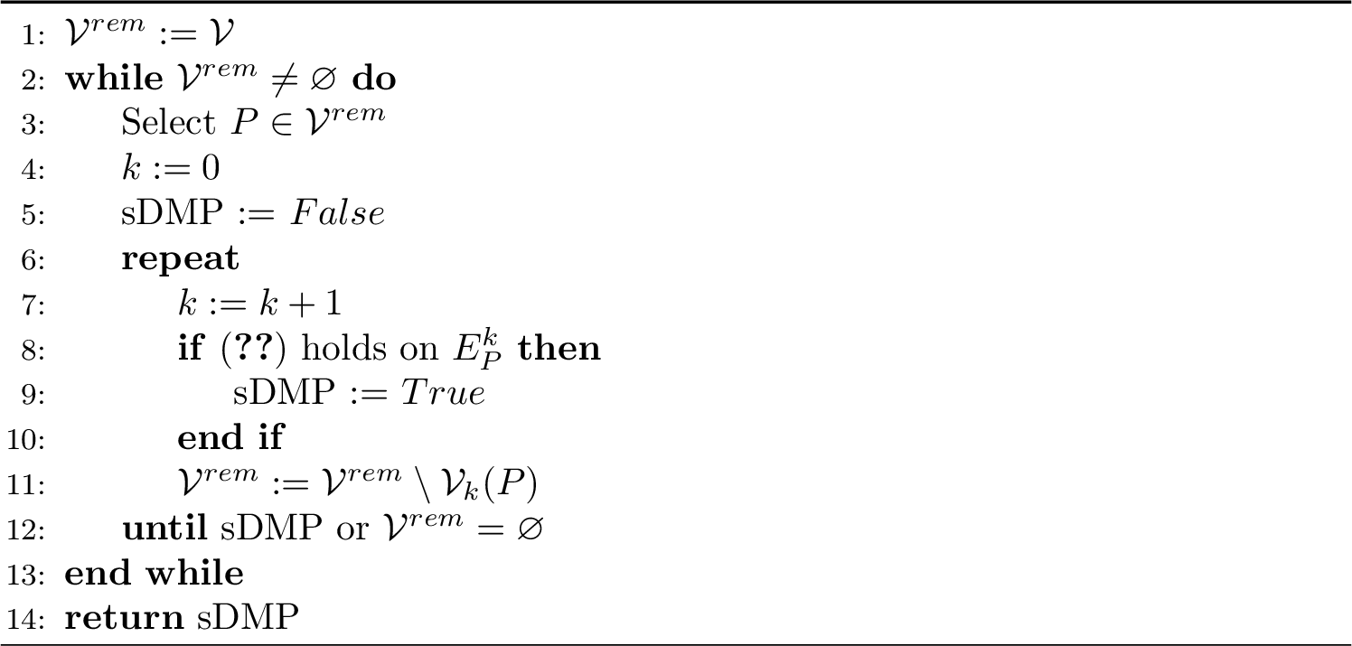
Algorithm 1 seeks to cover the domain \(D\) with patches of the form \(E^k_{P_i}\), \(k=1, 2, ...\), for some interior vertices \(P_i\), on which sDMP-A (or sDMP-B, respectively) is satisfied; the vertices \(P_i\) are the ones selected at line 3. In order to switch from sDMP-A to sDMP-B, one needs to replace 32 with 33 on line 8. Algorithm 1 will return “True” if sDMP holds, and “False” otherwise. The algorithm tracks the set of vertices that remain to be checked, which is denoted by \({\mathcal{V}}^{rem}\), a set that will become empty in finitely many steps, regardless of whether the variable “sDMP” becomes “True” or stays “False”. Cf. Corollary 2, if sDMP-A (or sDMP-B, respectively) fails on the entire domain \(D\), there must be at least one interior vertex \(P_{\mathrm{fail}}\) that does not lie in any patch \(E^k_{P}\) on which sDMP-A (or sDMP-B, respectively) holds. Hence, the point \(P_{\mathrm{fail}}\) will not be included in the “good” patches of any other vertex selected at line 3. Moreover, \(E^k_{P_{\mathrm{fail}}} = D\) for some \(k>0\), showing that the variable “sDMP”will remain “False” when returned. Thus, under the assumption of the connectivity of the graph of the interior vertices, Algorithm 1 always provides the correct answer on the validity of the sDMP for linear problems.
In terms of the complexity, the majority of the work goes into the test of line 8, where 32 (or 33 , respectively) is verified; that cost is \(O(N_k(P)^3)\) where \(N_k(P)\) is the cardinality of \({\mathcal{V}}_k(P)\), due to the necessity of computing the inverse of a matrix. For each selected \(P\), prior to completing the loop in lines 6–12, Algorithm 1 will run through line 8 for \(1, 2,\dots,k_P\). Hence, the cost of running the loop is \(O\left(\sum_{i=1}^{k_P} N_i(P)^3\right).\) If \(I_{\mathrm{DMP}}\) is the set of vertices selected at line 3, then the total cost is \[\label{eq:cost1} C_{Alg_1} = \sum_{P\in I_{\mathrm{DMP}}} O\left(\sum_{i=1}^{k_P} N_i(P)^3\right).\tag{34}\] Under additional assumptions, this leads to a simple, worst-case scenario, upper bound of the computational cost. Let \(k_{\max}\) be the largest value of \(k\) that appears on line 7 of Algorithm 1. Assuming quasi-uniformity of the mesh, we have \(N_k(P) \approx O(k^d)\). Hence, \[\label{eq:cost2} C_{Alg_1} = N \sum_{P\in I_{\mathrm{DMP}}} O\left(\sum_{i=1}^{k_{\max}} i^{3d}\right) = O(N k_{\max}^{3d+1}).\tag{35}\] The upper bound in 35 does not take into account the balance between a large \(k_{\max}\) and the size of \(I_{\mathrm{DMP}}\): if \(k_{\max}\) is relatively large there will be fewer calls to line 3 in the algorithm, which may lead to \(|I_{\mathrm{DMP}}| \ll N\). In the extreme case when sDMP is not satisfied, then it might even happen that \(|I_{\mathrm{DMP}}| = 1\), in case Algorithm 1 starts at \(P_{\mathrm{fail}}\). Hence the cost is just \(O(k_{\max}^{3d+1})\); since \(N = O(k^d_{\max})\), then the cost is \(O(N^{3+\frac{1}{d}})\). The last number is higher than verifying directly the sDMP on the entire mesh, which has a cost of \(O(N^3)\). However, if \(k^3_{\max} \ll N\) then Algorithm 1 is significantly more efficient than a direct verification. In particular, when mesh refinement leads to a small number of isolated irregularities, as shown in Section 5, then the cost is \(O(N)\).
3.4 Sufficient conditions for a weak discrete maximum principle↩︎
In this section we use a perturbation argument and sDMP-R property to prove wDMP-A for the linear elliptic equation under weaker conditions than in Corollary 2. This is relevant because there are standard meshes where the second inequality in 32 does not hold in its strict form.
The question of well-posedness of 14 under these conditions will certainly arise and be handled properly, but the current focus is on the relevant DMP.
Lemma 4. Consider the context and hypotheses of Lemma 3, except we now assume \(\tilde{c}\le 0\). If 28 holds, then \({\mathcal{S}}^D_h\) is well-posed and satisfies sDMP-R.
The proof follows closely that of Lemma 3.
Proof. Assume \(f\) is nonnegative. Since the matrix form of 14 is given, as in Lemma 3, by 29 , the first condition in 28 ensures that the linear equation 29 has a unique solution; hence, the problem is well-posed. Let \(\underline{u} = \min u_h^b = \min {\mathbf{u}}_\beta\). We assume \(\underline{u} \ge 0\). By taking \(r=\underline{u}\) in 31 we get \[\begin{align} {\mathbf{u}}_{\alpha} - \underline{u} {\mathbf{1}}_{\alpha} &=& \overbrace{-\: ({\mathbf{A}}_{\alpha \alpha} +{\mathbf{C}}_{\alpha \alpha})^{-1}({\mathbf{A}}_{\alpha \beta} + {\mathbf{C}}_{\alpha \beta})}^{> {\mathbf{0}}} \overbrace{({\mathbf{u}}_{\beta} - \underline{u} {\mathbf{1}}_{\beta})}^{\ge {\mathbf{0}}} \\ &&-\;\underline{u}\underbrace{({\mathbf{A}}_{\alpha \alpha} +{\mathbf{C}}_{\alpha \alpha})^{-1} ({\mathbf{C}}_{\alpha \alpha} {\mathbf{1}}_{\alpha} + {\mathbf{C}}_{\alpha \beta}{\mathbf{1}}_{\beta})}_{\le {\mathbf{0}}} + \underbrace{({\mathbf{A}}_{\alpha \alpha} +{\mathbf{C}}_{\alpha \alpha})^{-1}}_{>{\mathbf 0}}{\mathbf{F}}_{\alpha}\ge {\mathbf{0}}, \end{align}\] where we used \(\underline{u} \ge 0\) and \({\mathbf{C}}\le {\mathbf{0}}\). Therefore, \({\mathbf{u}}_{\alpha} - \underline{u} {\mathbf{1}}_{\alpha}\ge {\mathbf{0}}\); thus, \(\min {\mathbf{u}}_{\alpha} \ge \underline{u}\). If \({\mathbf{u}}_{\alpha} - \underline{u} {\mathbf{1}}_{\alpha}\) has a coordinate that is zero, then we have \[({\mathbf{u}}_{\beta} - \underline{u} {\mathbf{1}}_{\beta}) = {\mathbf{0}},\;\;{\mathbf{F}}_{\alpha} = {\mathbf{0}},\;\; \underline{u} ({\mathbf{C}}_{\alpha \alpha} {\mathbf{1}}_{\alpha} + {\mathbf{C}}_{\alpha \beta}{\mathbf{1}}_{\beta}) = {\mathbf{0}}.\] By applying 31 with \(r=\underline{u}\) we get \(({\mathbf{u}}_{\alpha} - \underline{u} {\mathbf{1}}_{\alpha}) = {\mathbf{0}}\), showing that \({\mathbf{u}}\) is constant. Hence, we proved that \({\mathcal{S}}^D_h\) satisfies sDMP-R. ◻
Theorem 6 (wDMP-A). Consider the common hypotheses and notation from Corollary 2, and assume \(\tilde{c}\equiv 0\). If for all \(i\in I\) we have \[\label{eq:matformWdmpAthm} {\mathbf{A}}_{\alpha_i \alpha_i}^{-1} > {\mathbf{0}}\;\;\;\mathrm{and}\;\;\;{\mathbf{A}}_{\alpha_i \beta_i} \le {\mathbf{0}},\tag{36}\] then \({\mathcal{S}}^{D}_h\) satisfies wDMP-A.
Note the similarity with the statement from Corollary 2; here we relaxed the second condition in 32 , and the conclusion is a weaker form of the DMP, namely wDMP-A.
Proof. We begin by defining a sequence of families of consistent discrete solution operators. This family would, in principle, be the finite element discretization of 1 2 with \({c}(x,u) = -\varepsilon u\) and \(\varepsilon>0\); however, neither the continuous, nor the discrete versions are guaranteed to be well-posed for a sufficiently rich family of \(\varepsilon>0\). In order to circumvent this problem, we restrict our attention to discrete solution operators, and only to a certain sequence \((\varepsilon_n)_{n\in \mathbb{N}}\) that converges to 0.
To define our solution operators first we note that the triangulation \({\mathcal{T}}_h\) is fixed. For every discrete subdomain \(E\subseteq D\) denote its sets of interior and boundary vertices by \(\alpha=\alpha(E)\) and \(\beta=\beta(E)\), respectively. Define the number \[\begin{align} \label{eq:setsigma} \delta = \min\bigcup_{E\subseteq D}\sigma({\mathbf{M}}_{\alpha(E) \alpha(E)}^{-1}{\mathbf{A}}_{\alpha(E) \alpha(E)}), \end{align}\tag{37}\] with the union being taken over all the discrete subdomains, and \(\sigma({\mathbf{B}})\) denoting the spectrum of a matrix \({\mathbf{B}}\). The expression in 37 is well defined because the set on the right-hand side above is finite. Moreover, since both \({\mathbf{M}}_{\alpha(E) \alpha(E)}\) and \({\mathbf{A}}_{\alpha(E) \alpha(E)}\) are symmetric positive definite matrices, the set in 37 lies in \((0,\infty)\), implying that \(\delta>0\). Let \(\varepsilon_n\) be a sequence so that \(0<\varepsilon_n<\delta\) and \(\lim_{n\to\infty }\varepsilon_n = 0\). Define \[\begin{align} {\mathbf{B}}^{(n)}_i = {\mathbf{A}}_{\alpha_i \alpha_i} - \varepsilon_n {\mathbf{M}}_{\alpha_i \alpha_i}. \end{align}\] Since \(\varepsilon_n\notin \sigma({\mathbf{M}}_{\alpha(E) \alpha(E)}^{-1}{\mathbf{A}}_{\alpha(E) \alpha(E)})\), it follows that \({\mathbf{B}}^{(n)}_i\) is invertible. Due to the continuity of matrix inversion we have the following: for all \(i\in I\) \[\begin{align} \lim_{n\to \infty} ({\mathbf{B}}^{(n)}_i)^{-1} = {\mathbf{A}}^{-1}_{\alpha_i \alpha_i} > {\mathbf{0}}. \end{align}\] Hence, there exists \(n_0\in \mathbb{N}\) so that for \[\label{eq:Bngzero} \forall n\ge n_0,\;\;\forall i\in I,\;\;({\mathbf{B}}^{(n)}_i)^{-1} > {\mathbf{0}}.\tag{38}\] It is assumed that \(\forall k\in \beta_i\), \(\exists j\in \alpha_i\) so that the boundary vertex \(P_k\) (of \(E_i\)) is connected to the interior vertex \(P_j\); this translates into \(({\mathbf{M}}_{\alpha_i \beta_i})_{jk}>0\), showing that every column of \({\mathbf{M}}_{\alpha_i \beta_i}\) has at least one positive entry. Since \({\mathbf{M}}_{\alpha_i \beta_i} \ge {\mathbf{0}}\), 38 implies that \[\begin{align} \label{eq:BnMnlzero1} \forall n\ge n_0,\;\;\forall i\in I,\;\; ({\mathbf{A}}_{\alpha_i \alpha_i} - \varepsilon_n {\mathbf{M}}_{\alpha_i \alpha_i})^{-1} {\mathbf{M}}_{\alpha_i \beta_i} > {\mathbf{0}}. \end{align}\tag{39}\] Therfore, it follows from 39 , 36 , and \(\varepsilon_n>0\) that \[\begin{align} \label{eq:BnMnlzero2} \;\;\;\forall n\ge n_0,\;\; \forall i\in I,\;\;({\mathbf{A}}_{\alpha_i \alpha_i} - \varepsilon_n {\mathbf{M}}_{\alpha_i \alpha_i})^{-1} ({\mathbf{A}}_{\alpha_i \beta_i}-\varepsilon_n{\mathbf{M}}_{\alpha_i \beta_i}) < {\mathbf{0}}. \end{align}\tag{40}\]
Now we construct the family of consistent solution operators, namely we consider the following sequence of discrete variational problems: given a discrete subdomain \(E\subseteq D\), find \(u_h\in V^h(\overline{E})\) of the form \(u_h = u_h^0+ u_h^b\) with \(u_h^0\in V_0^h(\overline{E})\), so that \[\begin{align} \label{eq:weakelldiscnegeps} a_E(u_h^0+u_h^b,v) -\varepsilon_n\left( u_h^0+u_h^b , v \right)_E=\left< f , v \right>_E,\;\;\forall v\in V_0^h(\overline{E}). \end{align}\tag{41}\] If \(\alpha=\alpha(E)\) and \(\beta=\beta(E)\), then 41 is formulated in matrix form as \[\begin{align} \label{eq:weakelldiscnegepsmat} ({\mathbf{A}}_{\alpha \alpha}-\varepsilon_n{\mathbf{M}}_{\alpha \alpha}){\mathbf{u}}_{\alpha} + ({\mathbf{A}}_{\alpha \beta} -\varepsilon_n{\mathbf{M}}_{\alpha \beta}){\mathbf{u}}_{\beta} = {\mathbf{F}}_{\alpha}. \end{align}\tag{42}\] The choice of \(\varepsilon_n\) ensures that 41 is well posed (uniquely solvable), hence this gives rise to a family of solution operators \({\mathcal{S}}^E_{h,n}: (V_0^h(\overline{E}))^*\times V^h(\partial E) \to V^h(E)\), so that \({\mathcal{S}}^E_{h,n}(f,u_{\beta}) = u = u_{\alpha}+u_{\beta}\), with \({\mathbf{u}}_{\alpha}\) and \({\mathbf{u}}_{\beta}\) satisfying 42 being the vector representations of \({u}_{\alpha}\) and \({u}_{\beta}\), respectively. Hence, Lemma 4 and 40 imply that for all \(i\in I\) and \(n\ge n_0\), \({\mathcal{S}}^{E_i}_{h,n}\) satisfies sDMP-R. Due to the variational formulation 41 , we can use an argument similar to that in Lemma 1 to show that for all \(n\ge n_0\), the family \(({\mathcal{S}}^E_{h,n})_{E\subseteq D}\) is consistent, as in Definition 1. Theorem 4(R) now applies to show that for all \(n\ge n_0\), \({\mathcal{S}}^{D}_{h,n}\) satisfies sDMP-R.
For the final step let \(f \in (V_0^h(\overline{D}))^*\) be nonnegative and \(u_h={\mathcal{S}}^{D}_{h}(f,u^b)\) be the solution of 14 with \(c\equiv 0\). Denote \[\begin{align} \underline{u} = \min_{\overline{D}} u_h,\;\;\; v_h = u_h-\underline{u}+1,\;\;\;\mathrm{and}\;\; v_h^b = u_h^b-\underline{u}+1. \end{align}\] Since \(c\equiv 0\), we have \(v_h={\mathcal{S}}^{D}_{h}(f,v_h^b)\), because the pair \({\mathbf{v}}_{\alpha}, {\mathbf{v}}_{\beta}\) given by \[{\mathbf{v}}_{\alpha} = {\mathbf{u}}_{\alpha}-(\underline{u}-1){\mathbf{1}}_{\alpha},\;\;\; {\mathbf{v}}_{\beta} = {\mathbf{u}}_{\beta}-(\underline{u}-1){\mathbf{1}}_{\beta},\] where \(\alpha=\alpha(D)\), \(\beta=\beta(D)\) satisfy 24 . This way we ensure \(v_h \ge 1\) (the number 1 is not special, all that matters is that \(1>0\)). Define \(v_{h,n}={\mathcal{S}}^{D}_{h,n}(f,v_h^b)\). Using 24 and 42 , we get \[\lim_{n\to\infty}v_{h,n} = v_h \ge 1\;\;\mathrm{in}\;\;V^h(D)\;\;\mathrm{(pointwise\;or\;any\;norm)},\] showing that \(\exists n_1\ge n_0\) so that for \(n\ge n_1\) we have \(v_{h,n}>0\). Since \({\mathcal{S}}^{D}_{h,n}\) satisfies sDMP-R, we get \[\label{eq:sdmprvn} \min_{\overline{D}} v_{h,n} = \min_{\partial{D}} v_{h,n} = \min_{\partial{D}} v^b_{h},\;\;\forall n\ge n_1.\tag{43}\] After passing to the limit in 43 we get \[\label{eq:sdmpru} \min_{\overline{D}} u_{h} = \min_{\overline{D}} v_{h} + \underbar{u}-1 = \min_{\partial{D}} v^b_{h} + \underbar{u}-1 = \min_{\partial{D}} u^b_{h},\tag{44}\] showing that \({\mathcal{S}}^{D}_{h}\) satisfies wDMP-A. ◻
4 Application to linear elliptic equations↩︎
We continue to restrict our attention to \({\mathcal{P}}_1\) finite elements. In this section we apply the results from Section 3 to the linear version of 14 , namely the case where \(c\) takes the form 7 . The focus is on the connection to classical results, the angle condition, and the violation of the strong DMP due to mesh properties at the boundary.
4.1 Connection to the classical results↩︎
In this section we revisit classical results for meshes where the classical angle condition 46 (or its weaker version) is satisfied. This is related to local DMPs holding on the smallest meaningful discrete units, namely the union of all triangles that contain a vertex.
Definition 3. We call \(E\subseteq D\) a connected discrete subdomain if the graph of the nodes that are interior to \(E\) is connected (using only interior edges), and every vertex on \(\partial E\) is connected to a vertex interior to \(E\).
The following is a variant of a classical result, which we prove here using the connectivity technique introduced in Section 3.
Theorem 7. Assume \(\tilde{c}\equiv 0\), and that the stiffness matrix \({\mathbf{A}}\) in 14 satisfies \({\mathbf{A}}_{ij}<0\) whenever the vertices \(P_i\) and \(P_j\) are adjacent with at least one of them lying in the interior (it does not need to hold if \(P_i,P_j\in \partial D\)). Then the discrete solution operator \({\mathcal{S}}^E_h\) satisfies sDMP-A for every connected discrete subdomain \(E\subseteq D\).
Note that this is the closest statement to the continuous case, where the maximum principle is satisfied on every qualifying subdomain.
Proof. Let \(E\subseteq D\) a connected discrete subdomain. For every vertex \(P_i\) interior to \(E\) we consider the set \(E_i = \bigcup \{T\in{\mathcal{T}}_h\; :\;P_i\in T\}\), which we call the star around \(P_i\). The boundary vertices of \(E_i\) are the adjacent vertices of \(P_i\), which is the only interior node of \(E_i\). In the terminology of Lemma 2, \(\alpha = \{i\}\) and \(\beta=\{j\;:\;{\mathbf{A}}_{ij}<0\}\), and the conditions 23 are satisfied in a trivial manner. Hence, \({\mathcal{S}}^{E_i}_h\) satisfies sDMP-A. Corollary 1 implies that \({\mathcal{S}}^{E}_h\) satisfies sDMP-A. ◻
4.2 The angle condition↩︎
For \({\mathcal{P}}_1\) elements, the condition \({\mathbf{A}}_{ij}<0\) for adjacent vertices \(P_i\) and \(P_j\) is known as the “angle condition,” and it is the backbone of the majority of results regarding DMPs, not just for \({\mathcal{P}}_1\) elements, but also for \({\mathcal{Q}}_1\) [7], [24], [25], \({\mathcal{P}}_2\) [26], and higher elements [8], [9]. The root of the name lies in the formula for the entries in the stiffness matrix for the Laplacian (\(a_{ji} = \delta_{ij}\) in 1 ); If \(P_i\) and \(P_j\) are adjacent vertices, denote by \({\mathcal{T}}_1\) and \({\mathcal{T}}_2\) the triangles bordered by the edge \(e=\overline{P_1 P_2}\), and let \(\theta_1, \theta_2\) be the angles opposite the edge \(e\) in each of \({\mathcal{T}}_1\) and \({\mathcal{T}}_2\), respectively (see Fig. 2, left). Cf. Lemma A.1. in [17], \[\label{eq:formula2triangle} {\mathbf{A}}_{ij} = a_D(\varphi_j,\varphi_i) = {\color{black}\int_{{\mathcal{T}}_1 \cup {\mathcal{T}}_2} \nabla \varphi_i \cdot \nabla \varphi_j} = -\frac{\sin (\theta_1+\theta_2)}{2 \sin \theta_1 \sin \theta_2}.\tag{45}\] Thus we arrive at the following angle condition: \[\label{eq:anglecond} {\mathbf{A}}_{ij} < 0\;\;\;\;\mathrm{iff}\;\;\;\; \theta_1+\theta_2 < \pi.\tag{46}\] We should also note the weaker condition: \({\mathbf{A}}_{ij} \le 0\) iff \(\theta_1+\theta_2 \le \pi\). Oftentimes the angle condition is remembered as “all angles must be acute”, a hypothesis that certainly implies 46 .
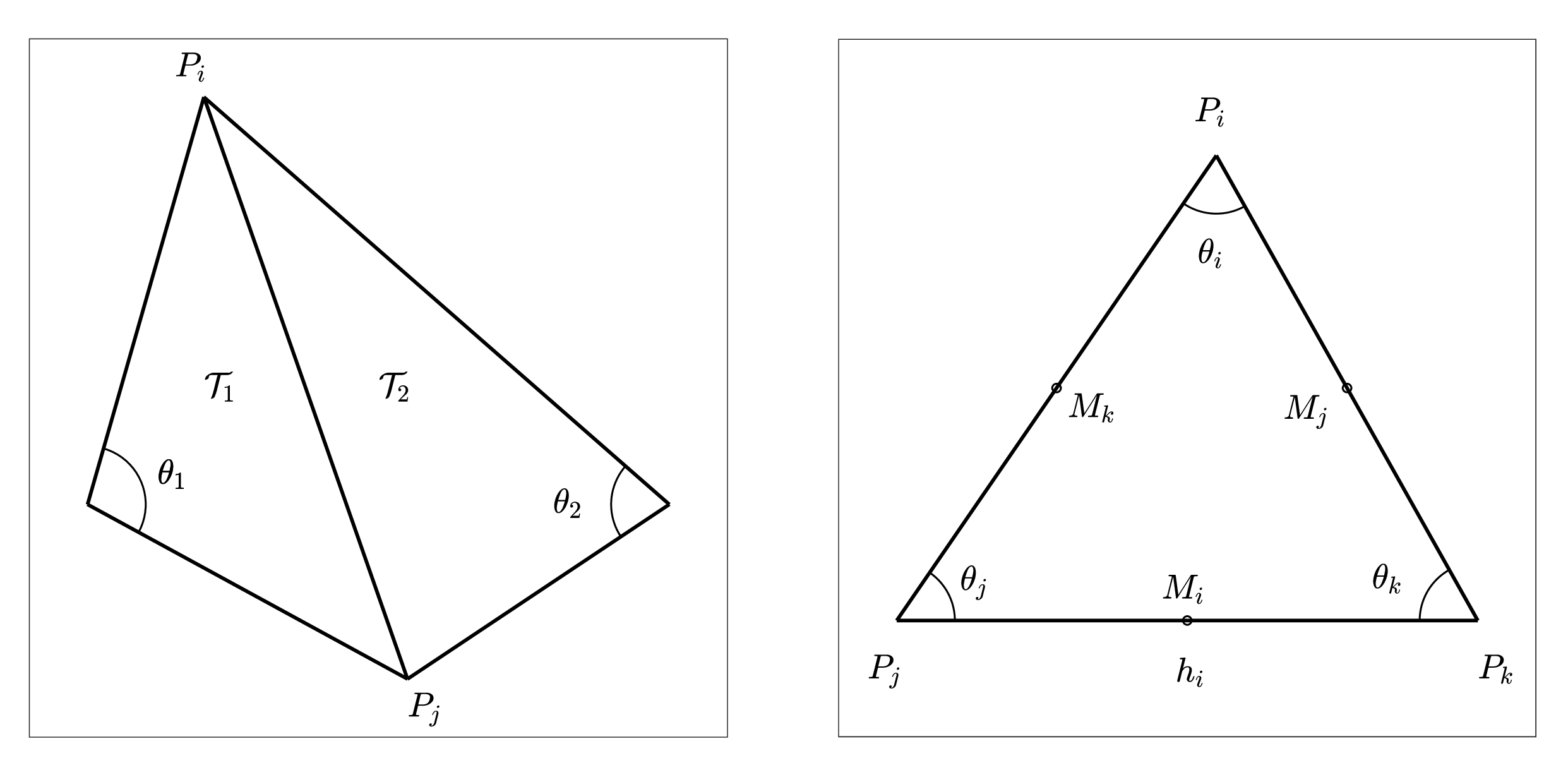
Figure 2: Triangle elements entering the formulas for stiffness and mass matrices..
We also recall from (see [17]) the formulas for the diagonal entries of the stiffness matrix \({\mathbf{A}}\). Consider a mesh triangle \({\mathcal{T}}\) with vertices \(P_i, P_j, P_k\) and angles \(\theta_i, \theta_j, \theta_k\) (refer to Fig. 2, right), and let \(\varphi_i\) be the basis function associated with \(P_i\). The contribution to \({\mathbf{A}}_{ii}\) from \({\mathcal{T}}\) is given by \[\label{eq:formula1triangle} \int_{{\mathcal{T}}}|\nabla \varphi_i|^2 = \frac{\sin \theta_i}{2 \sin \theta_j \sin \theta_k}.\tag{47}\] Fo the mass matrix we use the the fact that the cubature rule \[\begin{align} Q(f) = \frac{\mu({\mathcal{T}})}{3} \sum_{\ell\in\{i,j,k\}} f(M_{\ell}) \end{align}\] is exact for quadratics, where \(M_i, M_j, M_k\) are the edge midpoints (see Fig. 2, right), and \(\mu({\mathcal{T}})\) denotes the area of \({\mathcal{T}}\). The contributions of \({\mathcal{T}}\) to the \(i^{\mathrm{th}}\) row of the mass matrix are \[\begin{align} \tag{48} \int_{{\mathcal{T}}}\varphi_i^2 &=& \frac{\mu({\mathcal{T}})}{3} \sum_{\ell\in\{i,j,k\}}\varphi^2_i(M_{\ell}) = \frac{\mu({\mathcal{T}})}{6} = \frac{h_i^2}{12(\cot \theta_j + \cot \theta_k)},\\ \tag{49} \int_{{\mathcal{T}}}\varphi_i \varphi_j &=& \frac{\mu({\mathcal{T}})}{3} \sum_{\ell\in\{i,j,k\}} \varphi_i(M_{\ell})\varphi_j(M_{\ell}) = \frac{\mu({\mathcal{T}})}{12} = \frac{h_k^2}{24(\cot \theta_i + \cot \theta_j)}, \end{align}\] where we use the area formula (and permutations) \[\mu({\mathcal{T}}) = \frac{h_i^2}{2(\cot \theta_j + \cot \theta_k)}.\]
Note that there are standard meshes of interest containing edges \(\overline{P_i P_j}\) for which \({\mathbf{A}}_{ij} = 0\), where wDMP-A is known to hold. In Example 1 we analyze such a mesh which can be regarded as a limiting case of a mesh that satisfies sDMP-A (and sDMP-B).
4.3 Defects related to boundary mesh properties↩︎
We first consider defects associated to mesh properties at the boundary of the domain. To begin with, consider a mesh with a triangle \(T\) having two edges on the boundary, which meet at the boundary vertex \(P\). Let \(V_0^h(\overline{D})\) denote all piecewise linear functions that vanish on \(\partial D\). A function in \(\psi\in V^h(\overline{D})\) that satisfies \[a_D(\psi,v)+(c(\cdot,\psi),v)_D=0\] for all \(v\in V_0^h(\overline{D})\) is often referred to as a discrete harmonic function [18], [27].
Lemma 5. Let \(\phi\) denote the Lagrange basis function that is 1 at \(P\) and zero at all other vertices. Consider the variational problem defined in 12 . Then \[a_D(\phi,v)+(c(\cdot,\phi),v)_D=0\] for all \(v\in V_0^h(\overline{D})\). Thus \(\phi\) is discrete harmonic but supported in \(T\), and \(u_0\) defined by 14 is identically zero when \(f\equiv 0\).
Proof. For \(v\in V_0^h(\overline{D})\), the supports of \(v\) and \(\phi\) intersect in a set of measure zero, the third edge of \(T\). ◻
Example 1. Let the two-dimensional vectors be \({\mathbf{v}}_{\theta}=[\cos \theta, \sin \theta]^T\), so that \({\mathbf{v}}_0=[1, 0]^T\). For \(\pi/2
\le \theta< \pi\), define the rhombus \(D(\theta) = \{ s\: {\mathbf{v}}_0 + t\: {\mathbf{v}}_{\theta}\;:\;0 < s, t\;<1\}\). We consider the Poisson equation on \(D(\theta)\)
(\(a_{ji} = \delta_{ij}\) and \(c \equiv 0\) in 1 ). To obtain a triangular mesh we partition \(D(\theta)\) in \(n\times n\) identical rhombuses, which we further divide into triangles along their short diagonal, as pictured in Fig. 3 – right. Consider a standard lexicographic numbering of the
vertices, numbered from \(1\) to \(N=(n+1)\times (n+1)\). The case \(\theta = \pi/2\) leads to \(D(\theta) = [0,1]\times
[0,1]\) with the classical three-line mesh discretization, as shown in Fig. 3 – left.
Case 1: \(\theta >\pi/2\) (Fig. 3 – right). We first note that the boundary values imposed at the vertices \(P_{n+1} = (1,0)\) and
\(P_k = (\cos \theta,\sin\theta)\), with \(k = 1+ n (n+1)\), do not influence the solution in the interior; that is, \(u^0_h\) is the same regardless of the
values \(u^b_h(P_{n+1})\) and \(u^b_h(P_k)\). This shows \(S^D_h\) does not satisfy sDMP-A, since attaining a minimum for \(u_h^0\) in the interior does not imply \(u_h=u^0_h+u^b_h\) is constant. However, if \({\tilde{D}}\) denotes the domain \(D\)
from which we remove the triangles containing the vertices \(P_{n+1}\) and \(P_k\) (shaded in Fig. 3 – right), then \(S^{\tilde{D}}_h\) satisfies sDMP-A, since all the angles are acute, and every boundary node is connected to an internal node. Furthermore, if we now add back the triangles to the domain, then for any nonnegative \(f\) and discrete boundary function \(u^b_h\in V^h(\partial D)\), the interior part of the solution \(u^0_h\) satisfies
\[\begin{align}
\label{eq:wDMPrhombus}
\min_{P\in Int(D)} u^0_h(P) & =& \min_{P\in Int(\tilde{D})} u^0_h(P) \ge \min_{P\in \partial\tilde{D}} u^b_h(P)\\
& \ge& \min
\{\min_{P\in \partial\tilde{D}} u^b_h(P), u^b_h(P_{n+1}), u^b_h(P_k)\} = \min_{P\in \partial {D}} u^b_h(P).
\end{align}\tag{50}\] This shows that \(S^{{D}}_h\) satisfies wDMP-A. We will show in Section 6 that \(S^{\tilde{D}}_h\) also satisfies
sDMP-B when \(c\) is non-zero.
Case 2: \(\theta = \pi/2\) (Fig. 3 – left). In this case 45 implies that \({\mathbf{A}}_{ij}=0\)
for every edge \(\overline{P_i P_j}\) parallel to the line \(y=x\). This shows that the boundary values at all the four corners of \(D\) do not influence the
computed (interior) solution \(u^0_h\), so \(S^{{D}}_h\) does not satisfy sDMP-A. In this case even \(S^{\tilde{D}}_h\) does not satisfy sDMP-A due to the
values at \(P_1\) and \(P_N\) not influencing \(u^0_h\). This does not change by removing the triangles containing \(P_1\)
and \(P_N\), as doing so will give rise to new “disconnected” boundary vertices. However, Theorem 6 implies that \(S^{\tilde{D}}_h\) satisfies wDMP-A, as we choose for each interior point \(P_i\) the star \(E_i\) as in the proof of Theorem 7. Note that the hypotheses of Theorem 6 are satisfied, because we have
\[\label{eq:nonposent}
{\color{black}{\mathbf{A}}_{ij}\le 0},\;\;\mathrm{for\; all}\;\; i\ne j.\tag{51}\] The same calculation as in Case 1 shows that also \(S^{{D}}_h\) satisfies wDMP-A.
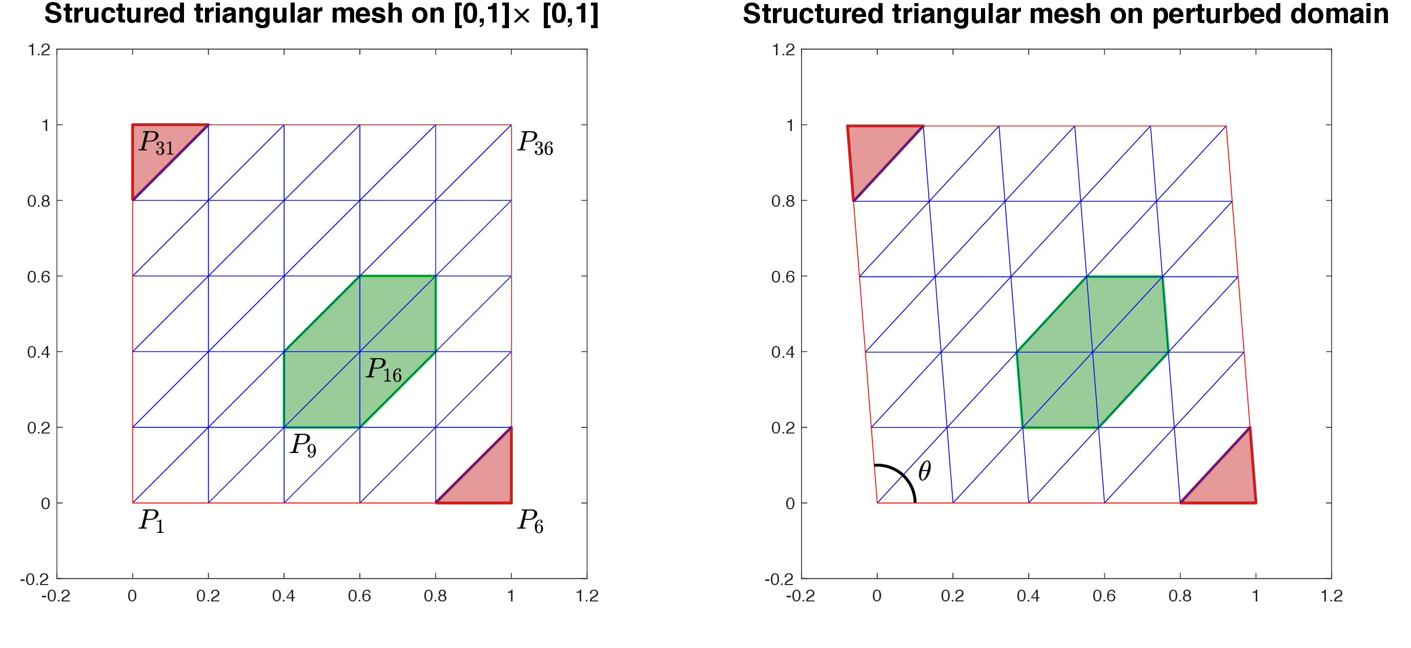
Figure 3: Left: The Poisson solution operator \(S^D_h\) satisfies wDMP-A on the classical three-line mesh on \(D = [0,1]\times[0,1]\) (here \(n=5\)), but does not satisfy sDMP-A; entries in the stiffness matrix corresponding to edges like \(\overline{P_9, P_{16}}\) are zero. Right: If \(\tilde{D}\) is obtained by removing from \(D\) the triangles containing \(P_6\) and \(P_{31}\), then sDMP-A holds on \(\tilde{D}\), and wDMP-A holds on \({D}\)..
5 Defects related to interior mesh properties↩︎
In this section we focus on the Poisson equation with a constant reaction rate \(\tilde{c}\); thus, the reaction matrix has the form \({\mathbf{C}} = \tilde{c}\: {\mathbf{M}}\). We present a set of examples where the angle condition 46 (which still refers to the stiffness matrix) fails for certain edges, and yet we can prove that the sDMP-A and sDMP-B hold, under appropriate assumptions.
5.1 A class of meshes with defects↩︎
For the purpose of this section we call edges where 46 fails “defects”. The domain is related to that in Example 1 via a 90 degree rotation, namely we consider a rhombus \(D(\theta)\) centered at the origin, with the long diagonal lying on the \(x\)-axis, and \(0<\theta < \pi/2\) representing the acute angle of the rhombus. We partition \(D(\theta)\) into \(n\times n\) identical rhombuses, which we further divide either along the short or the long diagonal, according to a set of rules described below. First, all the rhombuses that contain a boundary edge are divided along their short diagonal, as in Example 1. Second, we eliminate the two corner triangles that cross the \(x\)-axis (see Figures 4–9), and we denote by \(\tilde{D}(\theta)\) the remaining domain; note that \(\tilde{D}(\theta)\) changes as the mesh is refined. Third, the defects are selected from a finite library described below, and they need to be separated by triangles in which all the edges satisfy the angle condition 46 . Our presentation does not aim to exhaust all the possible patterns; instead, we want to showcase the usage our results on some nontrivial examples.
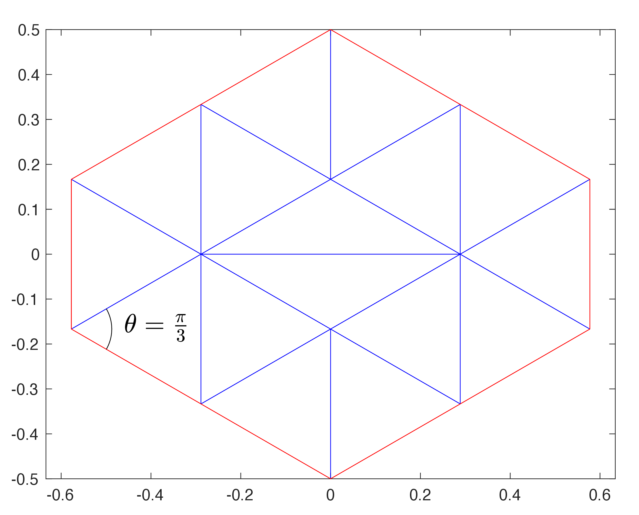
Figure 4: The mesh \(G_1(\pi/3)\) contains 1 edge violating the angle condition, but \({\mathbf{A}}^{-1}_1 >{\mathbf 0}\) (verified numerically – see also Fig. 7)..
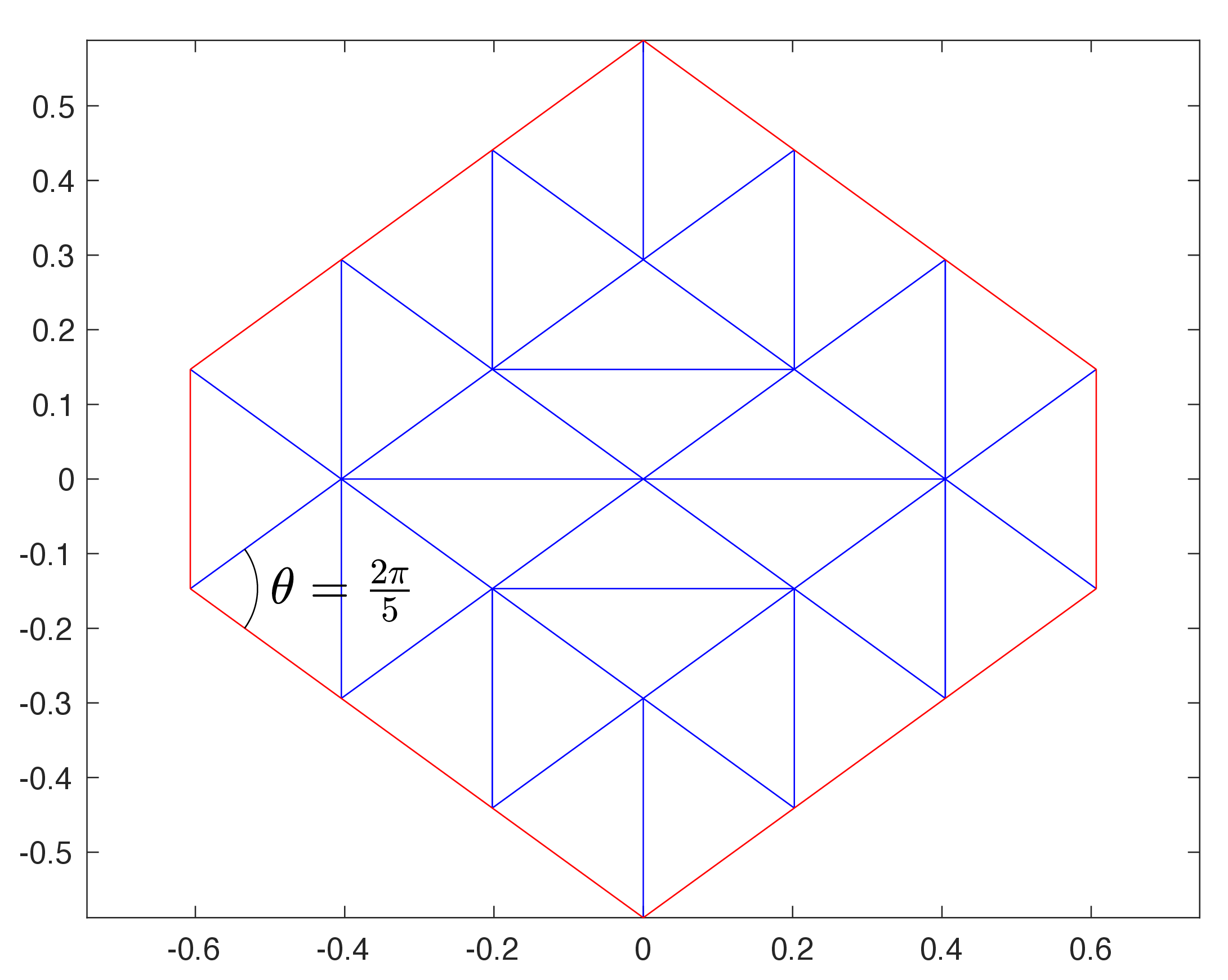
Figure 5: The mesh \(G_2(2\pi/5)\) contains 4 edges violating the angle condition, but \({\mathbf{A}}^{-1}_2 >{\mathbf 0}\) (verified numerically – see also Fig. 7)..
Example 2.
This example originates in [28]; in the context of homogeneous Dirichlet boundary conditions, it is shown that for a certain \(\varepsilon>0\) and \(\pi/2-\varepsilon <\theta < \pi/2\), the discrete Green’s function for \(D(\theta)\) cut into \(n\times n\) rhombuses and along their long diagonal is positive, independent of the number of subdivisions \(n\). Because in this setup the edges connecting to the boundary vertices are defects, the wDMP is not satisfied. Variations on this example are further discussed in [17], [29].
In our case, the defects are grouped into “mini” versions of the domain \({D}(\theta)\), namely, they are rhombuses made of \(k\times k\) elemental (smallest) rhombuses, all of which are divided along their long diagonal. Furthermore, we add to these domains a one-layer lining of elemental rhombuses that are divided along their short diagonal, and we eliminate the two extremal (on the \(x\)-axis) corner triangles. We call this mesh \(G_k(\theta)\), and we omit \(\theta\) when not necessary. In Fig. 4 we show \(G_1(\pi/3)\), and in Fig. 5 we show \(G_2(2\pi/5)\). Note that \(G_k\) contains \(k^2\) defective edges. We should point out that defects of these types may arise naturally in mesh refinement, e.g., when adding a midpoint to an edge and cutting the triangles adjacent along the medians – see Fig. 6. One can spot several such localized defects by carefully examining the refined meshes in Figure 6 from [30].
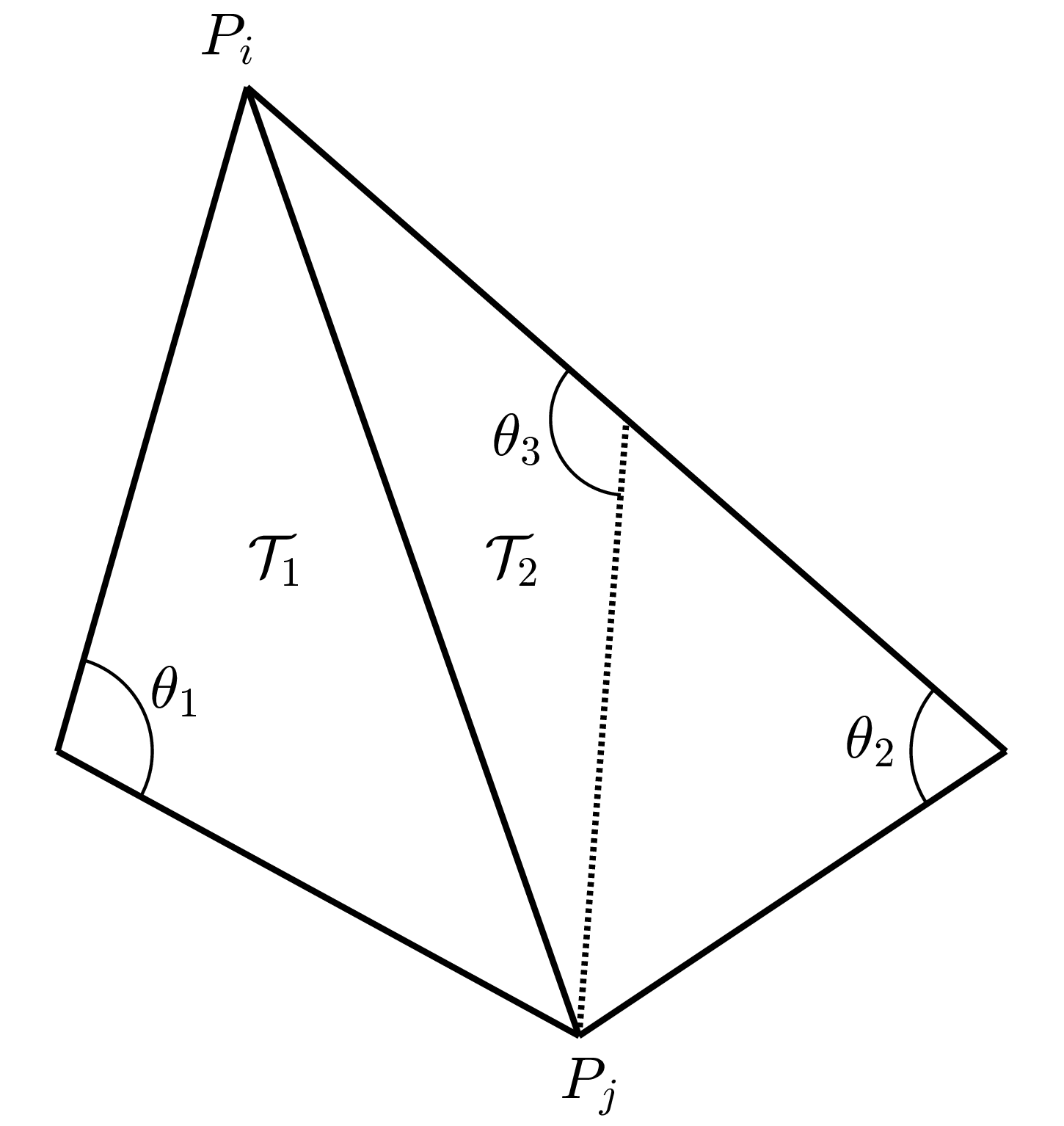
Figure 6: The angle condition holds for the original partition \({{\mathcal{T}}}_1\cup {{\mathcal{T}}}_2\), because \(\theta_1 + \theta_2 < \pi\). However, the bisection of an edge leads to \(\theta_1 + \theta_3 > \pi\), implying that the angle condition is violated, as this causes \(A_{ij}>0\) for the edge connecting \(P_i\) and \(P_j\)..
We now discuss the positivity of the discrete Green’s function, i.e., the inverse of the stiffness matrix \({\mathbf{A}}_k(\theta)\) associated with the interior nodes of the mesh \(G_k(\theta)\).
Lemma 6. Denote by \({\mathbf{A}}_k(\theta)\) the stiffness matrix associated with the interior nodes of the mesh \(G_k(\theta)\). Then for each \(k\in \mathbb{N}\) there exists \(0<\theta_k <\pi/2\) so that \[\label{eq:invGreenposGk} {\mathbf{A}}^{-1}_k(\theta) > {\mathbf{0}},\;\;\forall \;\;\theta_k < \theta \le \pi/2.\tag{52}\]
Proof. The argument lies in the analysis of the limit case, \(\theta=\pi/2\). A simple calculation using 45 and 47 shows that \({\mathbf{A}} = {\mathbf{A}}_k(\pi/2)\) is a scaled version of the matrix resulted from the standard five-point stencil (finite difference) discretization of the Laplacian on the unit square with zero-boundary conditions: \[\begin{align} {\mathbf{A}}_{ij} = \left\{ \begin{array}{cll} 4, 3,\; \mathrm{or}\;2&\;\mathrm{if}\;i=j&\;\mathrm{and}\;P_i\;\;\mathrm{interior, \;side,\;or\;corner\;vertex,\;resp.;}\\ -1,&\;\mathrm{if}\;i\ne j&\;\mathrm{and}\;\overline{P_i P_j}\;\;\mathrm{is\;an\;edge\;with\;slope\;}\pm 1. \end{array} \right . \end{align}\] Essentially, all the edges \(\overline{P_i P_j}\) in \(G_k(\pi/2)\) that are parallel to the \(x\)- or the \(y\)-axis (the diagonals of the small squares) yield \({\mathbf{A}}_{ij}=0\). It can easily be seen that \({\mathbf{A}}_k(\pi/2)\) is a Stieltjes matrix, meaning it is symmetric positive definite, satisfies 51 , and is irreducible. Cf. [16], \[\begin{align} {\mathbf{A}}^{-1}_k(\pi/2) > {\mathbf{0}}. \end{align}\] The result follows simply by continuity of the map \(\theta \mapsto {\mathbf{A}}^{-1}_k(\theta)\), namely we have \[\begin{align} \lim_{\theta \to \pi/2} {\mathbf{A}}^{-1}_k(\theta) = {\mathbf{A}}^{-1}_k(\pi/2) > {\mathbf{0}}, \end{align}\] which then implies 52 for some \(\theta_k<\pi/2\). ◻
In Fig 7 we plot the smallest value for \({\mathbf{A}}^{-1}_k(\theta)\) (computed numerically), for \(k = 1, 2, 3, 4\), and we see that is turns positive as \(\theta\to \pi/2\), thus supporting Lemma 6. It appears that \(\theta_1 < \theta_2 < \theta_3 < \theta_4\), although this is not essential for our arguments.
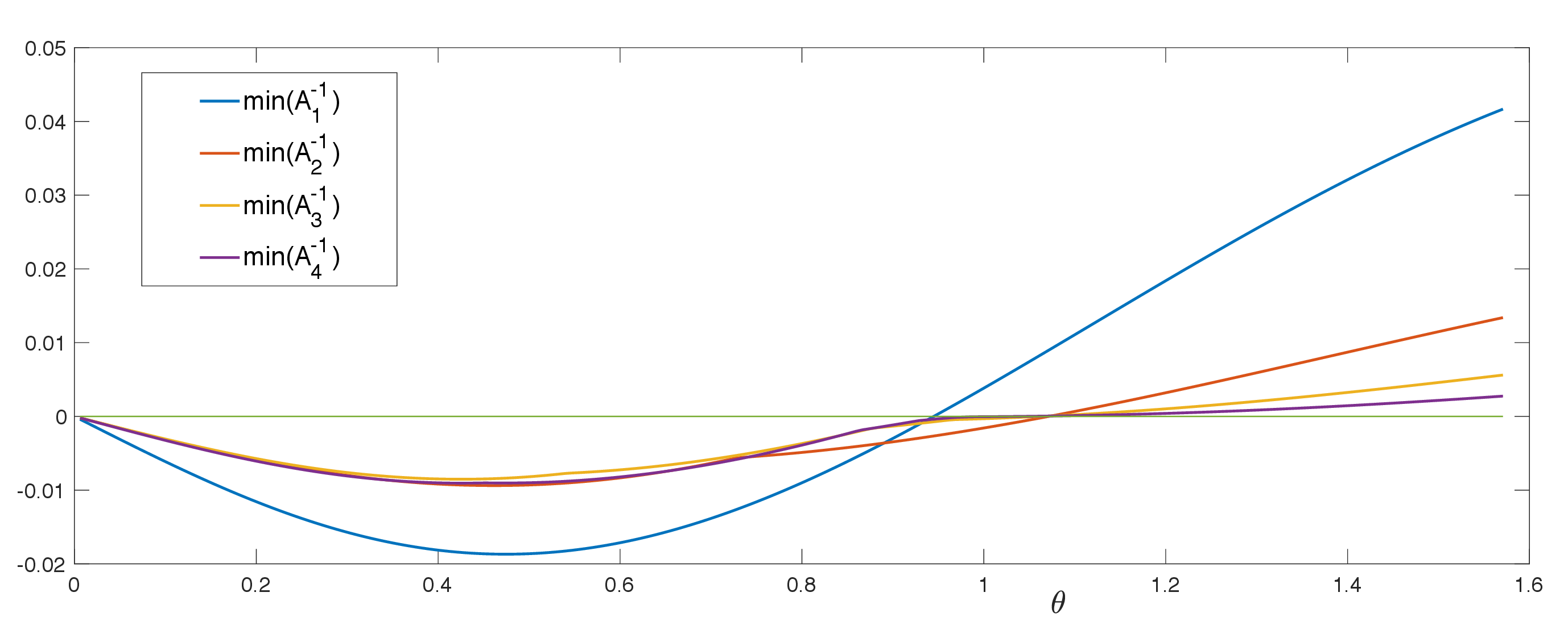
Figure 7: The smallest values of \({\mathbf{A}}^{-1}_1(\theta),\dots,{\mathbf{A}}^{-1}_4(\theta)\) are shown as functions of \(\theta\) (on the \(x\)-axis). Note that each of the four functions has a root \(\theta_k <\pi/2\) so that it is positive for \(\theta_k< \theta < \pi/2\)..
5.2 More complicated meshes↩︎
The next result describes a set of meshes on \({D}(\theta)\) for which various DMPs hold as \(h\to 0\).
Theorem 8. Let \(k\in \mathbb{N}\) and \(\theta\) so that \(\max_{\ell=1}^k\theta_{\ell} < \theta <\frac{\pi}{2}\). Consider a uniform
partition of \(D=D(\theta)\) in \(n\times n\) rhombuses, with each small rhombus being divided along either its long diagonal or its short diagonal, and let \(h\) be the mesh size. We assume that each interior vertex \(P\) lies in the interior of a mesh that is a scaled version of \(G_{\ell}(\theta)\) for some \(1\le \ell\le k\), or the star around \(P\) has only acute angles. (Examples of such meshes are given in Figures 8-9). Let
\(({\mathcal{S}}^E_h)_{E\subseteq D}\) be the consistent family of solution operators associated with the discrete linear variational problem 14 . Then the following hold:
(i) If \(\tilde{c}\equiv 0\), then the global solution operator \({\mathcal{S}}^{\tilde{D}}_h\) satisfies sDMP-A, and \({\mathcal{S}}^{{D}}_h\) satisfies wDMP-A.
(ii) If \(0\le \tilde{c}\le \tilde{c}_{\max}\), with \(\tilde{c}_{\max}\) a constant, then there exists \(h_{\max}>0\) depending on \(\theta\) and \(\tilde{c}_{\max}\) so that for \(0< h< h_{\max}\) the global solution operator \({\mathcal{S}}^{\tilde{D}}_h\) satisfies sDMP-B, and \({\mathcal{S}}^{D}_h\) satisfies wDMP-B.
Proof. For (i), the hypothesis implies that each interior vertex \(P\) lies either in the interior of a patch \(F_P\) that is a rescaled version of \(G_{\ell}(\theta)\), or in a star \(E_P\) (the union of the triangles having \(P\) as vertex) that has only acute angles. In the former case, since the stiffness
matrix in 2D is independent of the scale, Lemma 6 shows \({\mathbf{A}}^{-1}_{\ell} = {\mathbf{A}}^{-1}_{\ell}(\theta) >
{\mathbf{0}}\), hence the same holds for the stiffness matrix \({\mathbf{A}}_P\) associated with the interior vertices of \(F_P\), because \({\mathbf{A}}_P\) is identical to \({\mathbf{A}}_{\ell}\). Now let \({\mathbf{A}}^b_{\ell}={\mathbf{A}}^b_{\ell}(\theta)\) be the stiffness
matrix connecting interior and boundary entries in \(G_{\ell}(\theta)\), and \({\mathbf{A}}^b_P\) be its analogue on \(F_P\). Since the boundary layer of
\(F_P\) contains only edges that satisfy 46 , we have \(({\mathbf{A}}^b_P)_{ij}<0\) for every edge \(\overline{P_i P_j}\)
with \(P_i\in Int(F_P)\) and \(P_j\in \partial F_P\). This shows that \({\mathbf{A}}_P^{-1} {\mathbf{A}}^b_P < {\mathbf{0}}\), that is, 32 is verified for \(F_P\). For the latter case, when the patch is the star \(E_P\), the same argument as in Theorem 7 shows that 32 is verified on \(E_P\) as well. Corollary 2(i) shows that \({\mathcal{S}}^{\tilde{D}}_h\) satisfies sDMP-A. As in Example 1, adding the two corner triangles leads to \({\mathcal{S}}^{{D}}_h\) satisfying wDMP-A.
The argument for (ii) lies in the scaling of the mass matrix compared to that of the stiffness matrix. Assume a point \(P\) lies in the interior of a patch \(F_P\) that is a
rescaled version of \(G_{\ell}(\theta)\), as above. Denote by \({\mathbf{M}}_{\ell}={\mathbf{M}}_{\ell}(\theta)\) the mass matrix associated with the interior vertices of the reference mesh
\(G_{\ell}(\theta)\). Due to scaling (see 49 ), the associated mass matrix for \(F_P\) is \(K h^2{\mathbf{M}}_{\ell}\),
with \(K\) a dimensionless constant depending on \(\theta\) and \(\ell\). Similarly, if \({\mathbf{M}}^b_{\ell}={\mathbf{M}}^b_{\ell}(\theta)\) is the mass matrix connecting interior and boundary entries on \(G_{\ell}(\theta)\), then the analogous matrix on \(F_P\) is \(K h^2{\mathbf{M}}^b_{\ell}\). Hence, the interior and boundary reaction matrices \({\mathbf{C}}_P\) and \({\mathbf{C}}^b_P\), respectively, associated with \(F_P\) (see 22 ) satisfy \[\label{eq:masstozero}
{\mathbf{0}}\le {\mathbf{C}}_P \le K \tilde{c}_{\max} h^2{\mathbf{M}}_{\ell},\;\;\;{\mathbf{0}}\le {\mathbf{C}}^b_P \le K \tilde{c}_{\max} h^2{\mathbf{M}}^b_{\ell}.\tag{53}\] Consequently \[\begin{align}
\lim_{h\to 0} ({\mathbf{A}}_P + {\mathbf{C}}_P)^{-1} = {\mathbf{A}}_P^{-1} > {\mathbf{0}},
\end{align}\] and\[\begin{align}
\lim_{h\to 0} ({\mathbf{A}}_P + {\mathbf{C}}_P)^{-1}({\mathbf{A}}^b_P + {\mathbf{C}}^b_P) = {\mathbf{A}}_P^{-1}{\mathbf{A}}^b_P < {\mathbf{0}}.
\end{align}\] Hence, there exists \(h_{\max}>0\) depending on \(\tilde{c}_{\max}\) and \(K\) (which depends on \(\theta\) and \(k\) - the largest index of the defects), so that for \(0<h<h_{\max}\) we have \[\begin{align}
\label{eq:Cconditionsex1}
({\mathbf{A}}_P + {\mathbf{C}}_P)^{-1} > {\mathbf{0}},\;\;\mathrm{and}\;\;
({\mathbf{A}}_P + {\mathbf{C}}_P)^{-1}({\mathbf{A}}^b_P + {\mathbf{C}}^b_P) < {\mathbf{0}}.
\end{align}\tag{54}\] If, instead, the star \(E_P\) around \(P\) has only acute angles, similar inequalities hold if we replace \(F_P\) with
\(E_P\). By Corollary 2(ii), satisfies \({\mathcal{S}}^{\tilde{D}}_h\) satisfies
sDMP-B. The argument shown in Example 1 can be replicated to show that when adding back the two triangles at the horizontal extremes of \(\tilde{D}\), the global solution operator \({\mathcal{S}}^{{D}}_h\) satisfies wDMP-B. ◻
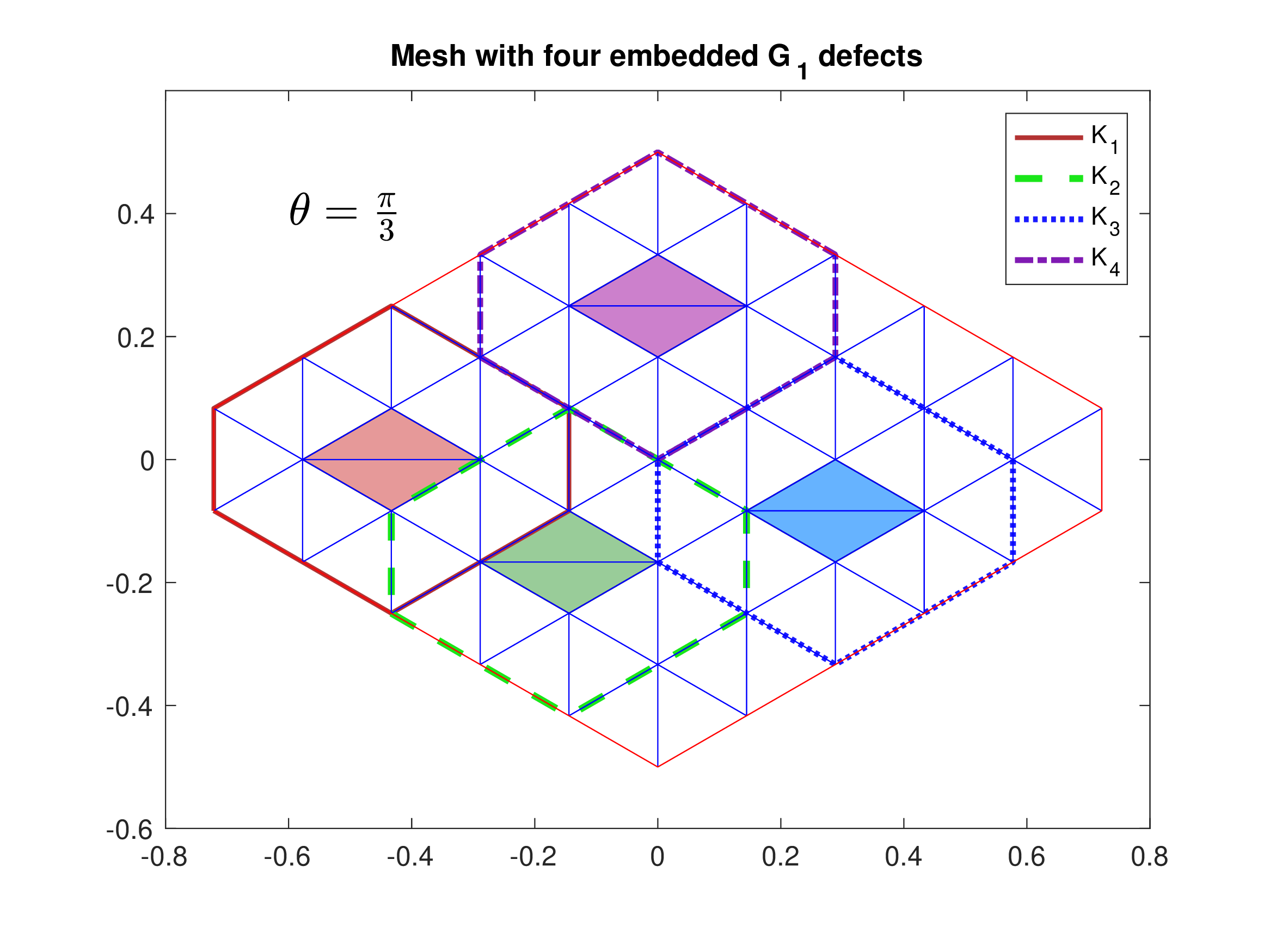
Figure 8: Mesh on \(\tilde{D}(\pi/3)\) with embedded \(G_1\) defects (\(k=1\) in reference to Theorem 8). The four domains which are similar to \(G_1\) are marked as \(K_1, \dots, K_4\)..
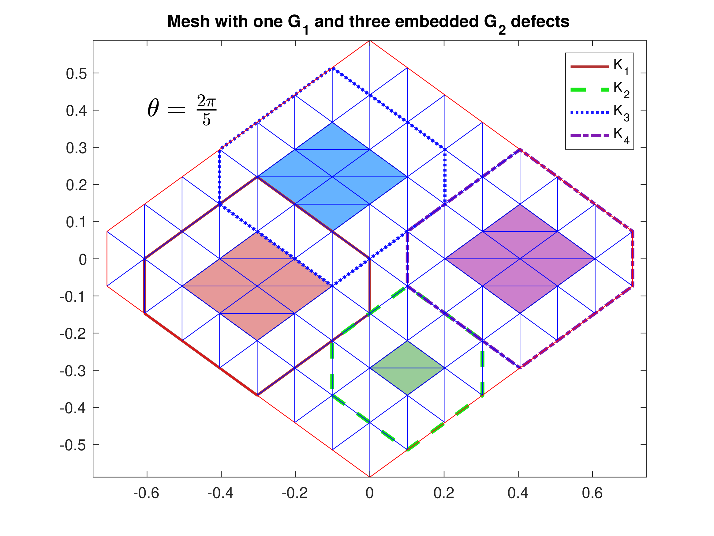
Figure 9: Mesh on \(\tilde{D}(2\pi/5)\) with embedded \(G_1\) and \(G_2\) defects (\(k=2\) in reference to Theorem 8). The four domains which are similar to \(G_1\) or \(G_2\) are marked as \(K_1, \dots, K_4\)..
5.3 wDMP-A for meshes with embedded nearly degenerate triangles↩︎
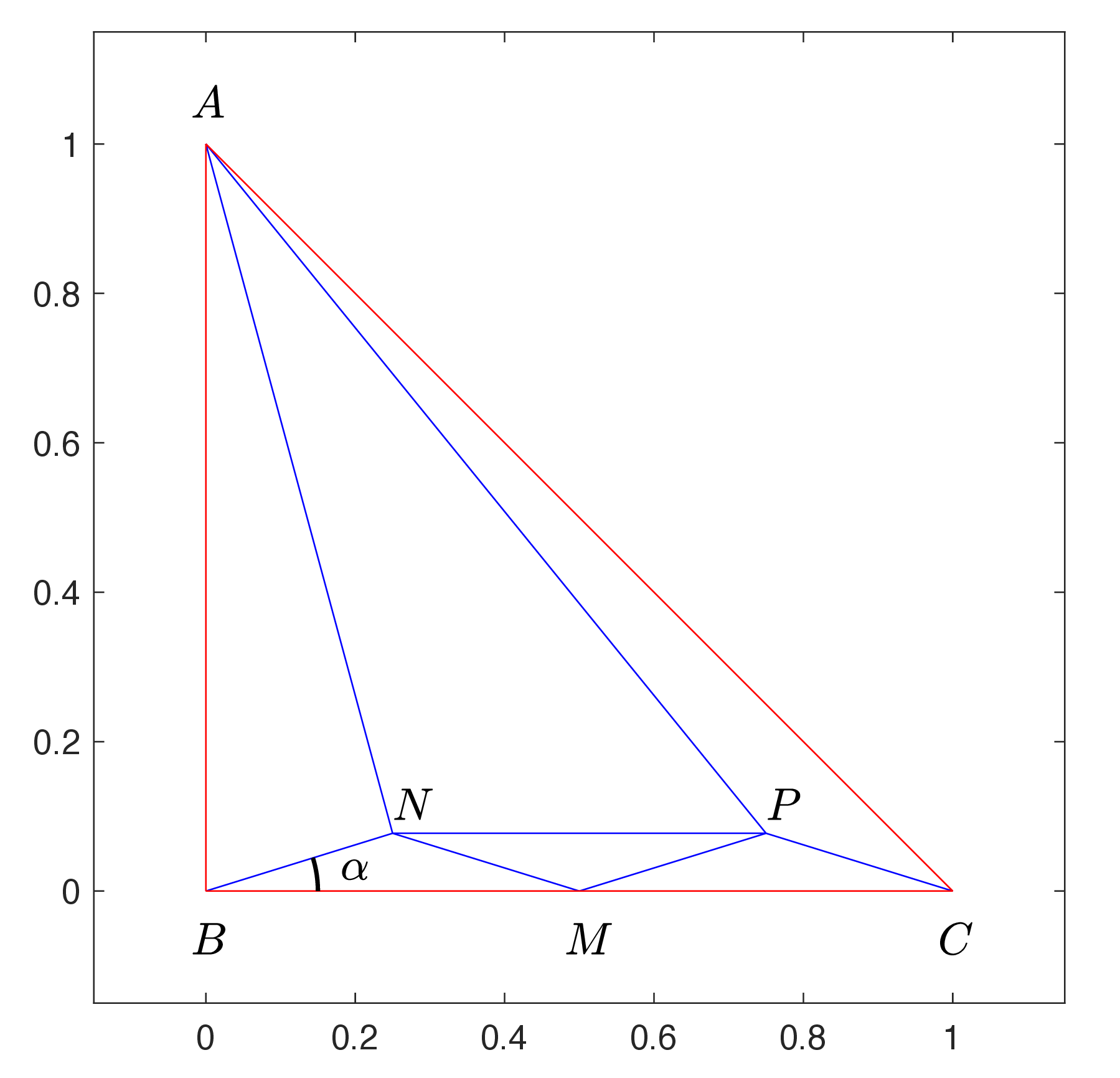
Figure 10: Triangle with nearly degenerate internal triangulation..
In this section we prove that the finite element solution operator for the Poisson equation satisfies the wDMP-A for a nearly degenerate mesh. This mesh is closely related to the example given in Section 5 in [17], in which a quasi-uniform triangulation is shown to violate the DMP as the mesh size \(h\to 0\), in the sense that the discrete Green’s function has provably negative values for all \(h>0\). The key element in both situations is the reference triangle \(\Delta A B C\), with \(A=(0,0), B=(0,1), C=(1,0)\), to which the following three points are added: \[\begin{align} &&M=\left(\frac{1}{2}, 0\right),\;\; N=\left(\frac{1}{4}, \frac{\tan \alpha}{4}\right),\;\; P=\left(\frac{3}{4}, \frac{\tan \alpha}{4}\right). \end{align}\] Together they give rise to the mesh shown in Fig. 10. The mesh on \(\Delta A B C\) violates the angle condition due to the fact that \(a(\phi_M, \phi_P)>0\) for a small enough angle \(\alpha>0\). In [17] \(\Delta A B C\) is placed at the boundary of a uniform three-line mesh similar to the one in Example 1 with \(\theta=\pi/2\), and it is shown that for a fixed, sufficiently small angle \(\alpha\) (refer to Fig. 10), the discrete Green’s function satisfies \(g_h^P(N)<0\) for all \(h>0\). By contrast, here we show that by placing \(\Delta A B C\) in the same type of mesh, just one element away from the boundary as in Fig. 11, the wDMP-A is satisfied for any \(0< \alpha < \alpha_0\) for a certain \(\alpha_0>0\). In fact, it can be placed anywhere inside the mesh, as long as it is surrounded by a layer of “good” triangles. It is instructive to compare the discrete Green’s functions between the cases when \(\Delta A B C\) is one layer inside a domain Fig. 12 (left) vs. right at the boundary Fig. 12 (right). We see in the bottom left corner of Fig. 12 that \(g^P_h >0\) inside the domain, and it has the expected shape of a Green’s function, while in the bottom right we have that \(g^P_h(N)<0\) (note the difference in the scales as well).
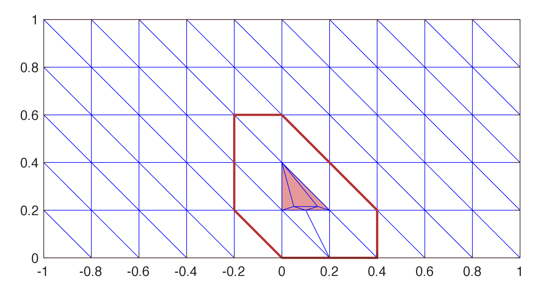
Figure 11: Uniform three-line mesh with an embedded, irregularly divided triangle one layer away from the boundary. The finite element solver for the Poisson equation satisfies the wDMP-A on this mesh, but fails to do so if the triangle is placed at the boundary..
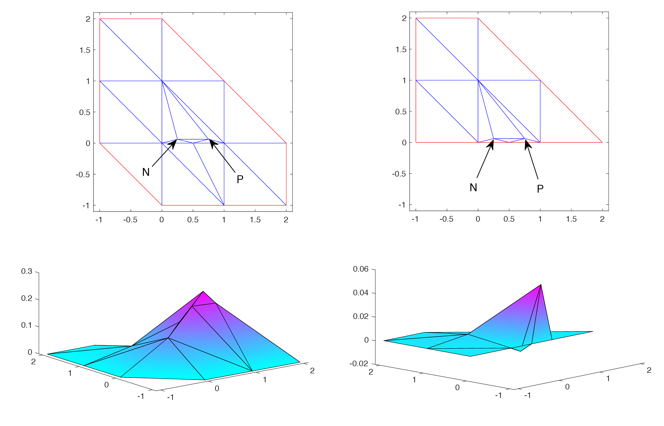
Figure 12: Green’s function for a mesh with near-degenerate elements near the boundary (left) vs. at the boundary (right); in the first case we have \(g_h^P(V)>0\) for any internal vertex \(V\), while in the second case \(g_h^P(N)<0\)..
The main argument is rooted in the analysis of the stiffness matrix for the subdomain \(E\) pictured in the top left corner of Fig. 12 (also in Figure 14), representing the union of the supports of the nodal basis functions associated with the vertices \(B, C, A, M, N, P\), in this order. Thus the ordered basis in the finite element space \({\mathcal{V}}\) of this subdomain is \({\mathcal{B}} = \{\varphi_B, \varphi_C, \varphi_A, \varphi_M, \varphi_N, \varphi_P\}\); we define \({\mathcal{V}} = \mathrm{span}({\mathcal{B}})\). The associated stiffness matrix is denoted by \({\mathbf{S}}={\mathbf{S}}(\alpha)\) (e.g., \({\mathbf{S}}_{11} = a_E(\varphi_B, \varphi_B)\), \({\mathbf{S}}_{35} = a_E(\varphi_A, \varphi_N)\), etc). The key result is the following.
Theorem 9. There exists a singular, rank-3 deficient matrix \({{\mathbf{T}}_0}>{\mathbf 0}\) so that \[\label{eq:limstiffex2} \lim_{\alpha\to 0} {\mathbf{S}}^{-1}(\alpha) = {\mathbf{T}}_0.\tag{55}\]
The proof of Theorem 9 is technical, but elementary; it is given in Appendix 8, where also the precise value for \({\mathbf{T}}_0\) is also shown. The theoretical result above was validated numerically. With regards to DMPs, the most remarkable part of Theorem 55 is the positivity of \({\mathbf{T}}_0\) as \(\alpha \to 0\). The existence of the limit as a bounded and singular matrix is related to the behavior of discrete Green’s functions on degenerate meshes. In order to better illustrate this behavior we provide a simpler case in Appendix 9, which emerged from an example discussed in [17] where the DMP holds on certain meshes violating the angle condition.
Corollary 3. There exists \(\alpha_0>0\) so that for \(\alpha\in (0,\alpha_0)\) we have \({\mathbf{S}}^{-1} > {\mathbf{0}}\).
Remark 10. Numerical results show that \({\mathbf{S}}^{-1} > {\mathbf{0}}\) for all \(\alpha>0\) for which the mesh is non-degenerate (see Figure 13).
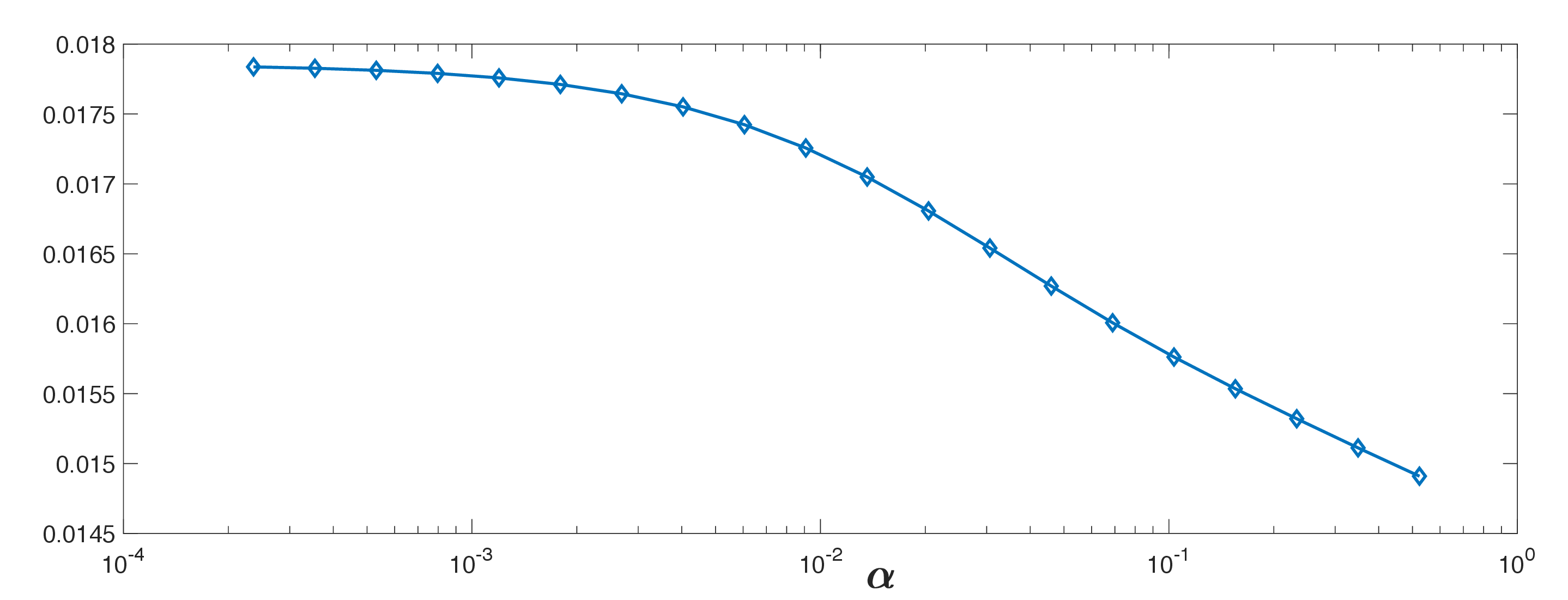
Figure 13: Smallest entry in \({\mathbf{S}}(\alpha)^{-1}\) for \(2.36 \times 10^{-4} < \alpha \le \pi/6\)..
Corollary 4. Consider the three-line mesh shown in Fig. 11 on a rectangle. We further partition any number of triangles so that the local mesh on each triangle is a scaled version of the mesh on \(\Delta ABC\) with \(0<\alpha<\alpha_0\). Moreover, assume any two such triangles are separated from each other and from the boundary by one layer of unpartitioned triangles. Then the finite element solution operator of the Poisson equation satisfies the wDMP-A on this mesh.
Proof. The statement follows from Corollary 3 and Theorem 6. The hypotheses ensure that every vertex \(V\) lies in the interior of a patch similar to \(E\) in the top left corner of Fig. 12, or the star around \(V\) is similar to a standard star in Example 1; in either case, the inequalities 36 are satisfied. ◻
6 The semilinear problem↩︎
In this section we prove a result for semilinear elliptic problems equations which is similar to Theorem 7. While results of this type can be found in a number of articles [5]–[7], [11]–[13], [31], [32], we will show that our technique is also applicable to prove sDMPs for semilinear elliptic equations. However, in this case we do assume off-diagonal entries of the stiffness matrix to be negative.
Theorem 11. Consider the discrete semilinear elliptic equation under the formulation 15 , and let \({c}\) satisfy 4 –6 . Furthermore, assume there is a constant \(C_A>0\) independent of \(h\) so that whenever vertices \(P_i\) and \(P_j\) are adjacent with at least one of them lying in the interior (that is, \(\overline{P_i P_j}\) is not a boundary edge), we have \({\mathbf{A}}_{ij}<0\) and \[\label{eq:stiffmatrixlimitsrat} {\mathbf{M}}_{ij}\le C_A h^2 |{\mathbf{A}}_{ij}|.\tag{56}\] Then there exists \(h_{\max}>0\) so that for all \(0<h<h_{\max}\), the discrete solution operator \({\mathcal{S}}^E_h\) of 15 satisfies sDMP-B for every connected discrete subdomain \(E\subseteq D\).
Proof. The argument follows the same path as in Theorem 7, namely we prove that \({\mathcal{S}}^E_h\) satisfies the sDMP-B for any star \(E_P\) around a vertex \(P\). The conclusion will follow from Corollary 1.
Thus, it is sufficient to prove the prove sDMP-B assuming the mesh has only one interior point \(P_1\) and boundary points \(P_2, \dots P_N\), i.e., \(D=E_{P_1}\). In this case \(h \le \mathrm{diam}(D) \le 2 h\); note that the mesh size plays a role in the estimation. Let \(u_h={\mathcal{S}}_h^D(f,u_h^b)\), and
denote \({\mathbf{F}}_i = f(P_i)\), \({\mathbf{U}}_i = u_h(P_i)\), for \(1\le i\le N\). In matrix terms, 15 is
represented by the nonlinear scalar equation: find \({\mathbf{U}}_1 \in \mathbb{R}\) so that \[\begin{align}
\label{eq:sldiscmat}
{\mathbf{A}}_{11} {\mathbf{U}}_1 + \sum_{i=2}^N {\mathbf{A}}_{i1}{\mathbf{U}}_i + {\mathbf{M}}_{11} \:c(P_1, {\mathbf{U}}_1) + \sum_{i=2}^N {\mathbf{M}}_{i1}\:c(P_i, {\mathbf{U}}_i)
= \sum_{i=1}^N {\mathbf{M}}_{i1} {\mathbf{F}}_i.
\end{align}\tag{57}\] Since \(f\ge 0\), we have \[\begin{align}
\label{eq:sldiscmatineq}
{\mathbf{A}}_{11} {\mathbf{U}}_1 + \sum_{i=2}^N {\mathbf{A}}_{i1}{\mathbf{U}}_i + {\mathbf{M}}_{11} \:c(P_1, {\mathbf{U}}_1) + \sum_{i=2}^N {\mathbf{M}}_{i1}\:c(P_i, {\mathbf{U}}_i) \ge 0.
\end{align}\tag{58}\] Note that \({\mathbf{A}}_{11}>0\), and \({\mathbf{M}}_{i1}>0\) for \(1\le i \le N\). We consider two cases:
Case 1: First assume that \({\mathbf{U}}_i\ge 0\) for \(2\le i\le N\), which implies that \[\label{eq:posClip}
0\le c(P_i, {\mathbf{U}}_i)\le L_c\: {\mathbf{U}}_i,\;\;2\le i\le N.\tag{59}\] In this case we have \[-\max_{\partial D}{u^-_h} = -\max_{2\le i\le N} {\mathbf{U}}_i^- = 0.\] If we had \({\mathbf{U}}_1<0\), then \(c(P_1, {\mathbf{U}}_1)\le 0\). Hence, \[\begin{align}
\nonumber
&&0<{\mathbf A}_{11} (-{\mathbf{U}}_1) - {\mathbf{M}}_{11} \:c(P_1, {\mathbf{U}}_1) \stackrel{\eqref{eq:sldiscmatineq}}{\le}
\sum_{i=2}^N {\mathbf{A}}_{i1}{\mathbf{U}}_i + \sum_{i=2}^N {\mathbf{M}}_{i1}\:c(P_i, {\mathbf{U}}_i)\\
\nonumber
&&\stackrel{\eqref{eq:posClip}}{\le} \sum_{i=2}^N ({\mathbf{A}}_{i1} + L_c{\mathbf{M}}_{i1}){\mathbf{U}}_i
=\sum_{i=2}^N (-{\mathbf{A}}_{i1})(-1 + L_c{\mathbf{M}}_{i1}/(-{\mathbf{A}}_{i1})){\mathbf{U}}_i\\
\label{eq:case1ineq}
&&\stackrel{\eqref{eq:stiffmatrixlimitsrat}}{\le}
\sum_{i=2}^N (-{\mathbf{A}}_{i1})(-1 + L_c C_A h^2){\mathbf{U}}_i.
\end{align}\tag{60}\] This is not possible if \(h<h_0 = \sqrt{(L_c C_A)^{-1}}\), for in that case we have \[\label{eq:case1ineq2}
(-{\mathbf{A}}_{i1})(-1 + L_c C_A h^2) < 0,\;\;\forall i=2,\dots,N.\tag{61}\] Together with \({\mathbf{U}}_i\ge 0\) for \(2\le i\le N\), this renders the sum in 60 to be nonpositive, contradicting our assumption on \({\mathbf{U}}_1\). It remains that \({\mathbf{U}}_1\ge 0\). For the strong part, assume \({\mathbf{U}}_1 = 0\); then we also have \(c(P_1, {\mathbf{U}}_1) = 0\). Using the same line of arguments as above, it follows that the sum from 60 is nonnegative.
However, since all the terms in 60 are nonpositive, they all must be zero, forcing \({\mathbf{U}}_i = 0\) for \(i=2,\dots,N\).
Case 2: We assume that at least one of the values \({\mathbf{U}}_i\), \(i=2, \dots N\) is negative. We partition \(I_N = \{2,\dots,N\} =
{\mathcal{N}}_{-}\cup {\mathcal{N}}_{+}\), with \[\begin{align}
{\mathcal{N}}_{-} = \{i\in I_N :\;{\mathbf{U}}_i< 0\},\;\;{\mathcal{N}}_{+} = \{i\in I_N :\;{\mathbf{U}}_i\ge 0\}.
\end{align}\] This implies \(c(P_i, {\mathbf{U}}_i)\le 0\) for \(i\in {\mathcal{N}}_{-}\), and \(c(P_i, {\mathbf{U}}_i)\ge 0\) for \(i\in {\mathcal{N}}_{+}\). Note that \[\begin{align}
\label{eq:acoeffineq}
-{\mathbf{A}}_{11} - \sum_{i\in {\mathcal{N}}_{-}} {\mathbf{A}}_{i1} = \sum_{i\in {\mathcal{N}}_{+}} {\mathbf{A}}_{i1} \le 0,
\end{align}\tag{62}\] because \(\sum_{i = 1}^N{\mathbf{A}}_{1i}=0\). Note that all the arguments still hold if \({\mathcal{N}}_+=\varnothing\). If \({\mathbf{U}}_1 < \min_{i\in {\mathcal{N}}_{-}} {\mathbf{U}}_i<0\), then cf. 58 we have \[\begin{align}
& \sum_{i\in {\mathcal{N}}_{+}} {\mathbf{A}}_{i1}{\mathbf{U}}_i + {\mathbf{M}}_{11} \:c(P_1, {\mathbf{U}}_1) + \sum_{i=2}^N {\mathbf{M}}_{i1}\:c(P_i, {\mathbf{U}}_i) \ge
-{\mathbf{A}}_{11} {\mathbf{U}}_1 + \sum_{i\in {\mathcal{N}}_{-}} (-{\mathbf{A}}_{i1}){\mathbf{U}}_i\\
& =
\underbrace{(-{\mathbf{A}}_{11} -\sum_{i\in {\mathcal{N}}_{-}} {\mathbf{A}}_{i1}) {\mathbf{U}}_1}_{\ge 0} + \sum_{i\in {\mathcal{N}}_{-}} (-{\mathbf{A}}_{i1})({\mathbf{U}}_i-{\mathbf{U}}_1)\ge
\sum_{i\in {\mathcal{N}}_{-}} (-{\mathbf{A}}_{i1})({\mathbf{U}}_i-{\mathbf{U}}_1) >0.
\end{align}\] Therefore, \[\begin{align}
\nonumber
&0< {\mathbf{M}}_{11} \:c(P_1, {\mathbf{U}}_1) + \sum_{i\in {\mathcal{N}}_{+}} \left({\mathbf{A}}_{i1}{\mathbf{U}}_i+{\mathbf{M}}_{i1}\:c(P_i, {\mathbf{U}}_i) \right) +
\sum_{i\in {\mathcal{N}}_{-}} {\mathbf{M}}_{i1}\:c(P_i, {\mathbf{U}}_i)\\
\label{eq:sldiscmatineqcase3}
&\stackrel{\eqref{eq:stiffmatrixlimitsrat}}{\le}
{\mathbf{M}}_{11} \:c(P_1, {\mathbf{U}}_1) +
\sum_{i\in {\mathcal{N}}_{+}} (-{\mathbf{A}}_{i1})(-1 + L_c C_A h^2){\mathbf{U}}_i +
\sum_{i\in {\mathcal{N}}_{-}} {\mathbf{M}}_{i1}\:c(P_i, {\mathbf{U}}_i).
\end{align}\tag{63}\] Following 61 , all the terms in the sum of 63 are nonpositive for \(h<h_0\), thus contradicting the assumption
on \({\mathbf{U}}_1\). Hence, \[\label{eq:minu0}
{\mathbf{U}}_1 \ge \min_{i\in {\mathcal{N}}_{-}} {\mathbf{U}}_i = -\max_{\partial E_{P_1}} u_h^-.\tag{64}\] If equality holds in 64 , then we have \({\mathbf{U}}_i-{\mathbf{U}}_1 \ge
0\), \(c(P_i, {\mathbf{U}}_i)-c(P_i, {\mathbf{U}}_1) \ge 0\), and \(c(P_i, {\mathbf{U}}_1)\le 0\) for \(1\le i \le N\). Consequently,
\[\begin{align}
\label{eq:sldiscmatineq4}
&0\le {\mathbf{A}}_{11}{\mathbf{U}}_1 + \sum_{i=2}^N {\mathbf{A}}_{i1}{\mathbf{U}}_i + \sum_{i=1}^N{\mathbf{M}}_{i1}\:c(P_i,{\mathbf{U}}_i) \\
&= \sum_{i=2}^N {\mathbf{A}}_{i1}({\mathbf{U}}_i-{\mathbf{U}}_1) + \sum_{i=1}^N{\mathbf{M}}_{i1}\:c(P_i,{\mathbf{U}}_1) +
\sum_{i=2}^N{\mathbf{M}}_{i1}\:\left(c(P_i,{\mathbf{U}}_i) - c(P_i, {\mathbf{U}}_1)\right)\\
&\le \sum_{i=2}^N ({\mathbf{A}}_{i1}+ L_c {\mathbf{M}}_{i1})({\mathbf{U}}_i-{\mathbf{U}}_1) + \sum_{i=1}^N{\mathbf{M}}_{i1}\:c(P_i,{\mathbf{U}}_1)\\
&\le \sum_{i=2}^N (-{\mathbf{A}}_{i1})(-1 + L_c C_A h^2 )({\mathbf{U}}_i-{\mathbf{U}}_1) + \sum_{i=1}^N{\mathbf{M}}_{i1}\:c(P_i,{\mathbf{U}}_1).
\end{align}\tag{65}\] Since all the terms in the sum above are nonpositive for \(h<h_0\), it follows that they are all zero, showing that \({\mathbf{U}}\) is constant and
that \(c(P_i,{\mathbf{U}}_1) = 0\) for \(1\le i\le N\). ◻
Remark 12. Condition 56 is related to the scaling of the mass matrix entries vs. those of the stiffness matrix: when scaling an element in \(\mathbb{R}^d\) by a factor \(h\), the mass matrix scales by \(h^d\), and the stiffness matrix by \(h^{d-2}\). Therefore 56 holds on the all uniform meshes \(G_k(\theta)\) in Section 5, with \(C_A\) depending on the angle \(\theta\), but not on \(k\). In general, condition 56 is related to the regularity of the mesh.
For the two-dimensional Laplacian on non-uniform meshes we can show that 56 is satisfied provided there exists \(\alpha_0>0\) so that \[\label{eq:accute95angle95lim} \alpha_0\le \alpha \le \frac{\pi}{2}-\alpha_0.\tag{66}\] Indeed, given an interior edge \(\overline{P_i P_j}\) in the notation from Section 4.1 and referring to Fig. 2 (right) we have cf. 49 \[\int_{\Delta P_i P_j P_k}\varphi_i \varphi_j = \frac{h_k^2}{24(\cot \theta_i + \cot \theta_j)} \le \frac{h_k^2}{48 \cot\left(\frac{\pi}{2}-\alpha_0\right)} = \frac{h_k^2}{48\tan \alpha_0},\] where \(h_k = |\overline{P_i P_j}|\). Since two adjacent triangles contribute to \({\mathbf{M}}_{ij}\), we have \[{\mathbf{M}}_{ij} \le \frac{h_k^2}{24\tan \alpha_0}.\] Using 45 and the notation in Figure 2 (left), we have \[-{\mathbf{A}}_{ij} = \frac{\sin (\theta_1+\theta_2)}{2 \sin \theta_1 \sin \theta_2} = \frac{1}{2}(\cot \theta_1+\cot \theta_2) \ge \cot \left(\frac{\pi}{2}-\alpha_0\right) = \tan \alpha_0.\] It follows that \[{\mathbf{M}}_{ij} \le \frac{h_k^2\tan\alpha_0}{24 \tan^2\alpha_0} \le \frac{h_k^2}{24 \tan^2\alpha_0}\:|{\mathbf{A}}_{ij}|.\] Hence, \(C_A = (24 \tan^2\alpha_0)^{-1}\).
7 Conclusions↩︎
We have introduced a novel technique for proving the global sDMP for elliptic equations; this can take two forms, depending on the presence or absence of the zeroth order term. This method does not assume that all the off-diagonal entries of the stiffness matrix are nonpositive. We applied this technique to the \({\mathcal{P}}_1\) discretization of elliptic equations, and showed that the global sDMP can hold even in the absence of the local sDMP is being satisfied everywhere. The method is also applied to prove – in a fairly natural fashion – that the sDMP holds for semilinear elliptic equations as well. As formulated, we believe the new method can be applied to other classes of nonlinear elliptic equations, as well as \(P_2\) and \(Q_1\) discretizations. The idea of local to global extension of DMPs via graph connectivity can be applied to other classes of problems, such as finite element discretizations of parabolic equations, and perhaps other types of discretizations of elliptic equations as well.
8 The proof of Theorem 9↩︎
Following a strategy similar to the one in [17], we use a hierarchical basis to compute an approximation to the matrix \({\mathbf{S}}={\mathbf{S}}(\alpha)\), which will lead to showing that \({\mathbf{S}}^{-1}>{\mathbf 0}\) for sufficiently small \(\alpha>0\). More precisely, we consider the coarse mesh on the domain \(E\) resulted from removing the points \(M, N, P\) (refer to Figure 14); the coarse basis functions we use are \(\widetilde{\varphi}_B, \widetilde{\varphi}_C, \widetilde{\varphi}_A\), all of which are linear on the entire triangle \(\Delta ABC\). The alternative basis in \({\mathcal{V}}\) is \(\widetilde{{\mathcal{B}}} = \{\widetilde{\varphi}_B, \widetilde{\varphi}_C, \widetilde{\varphi}_A, \varphi_M, \varphi_N, \varphi_P\}\), and we denote by \(\widetilde{{\mathbf{S}}}\) the stiffness matrix computed in the basis \(\widetilde{{\mathcal{B}}}\).
If \({\mathbf{A}}={\mathbf{A}}(\alpha), {\mathbf{B}}={\mathbf{B}}(\alpha)\) are nonsingular square matrices of the same size, we use the notation \({\mathbf{A}} \approx {\mathbf{B}}\) if \({\mathbf{A}} = {\mathbf{B}}({\mathbf{I}} + {\mathbf{O}}(\alpha))\) for sufficiently small \(\alpha\), where \({\mathbf{O}}(\alpha)\) is a matrix with entries of size \(O(\alpha)\). It is a simple exercise to see that this an equivalence relation which is closed to matrix product and inversion, in the sense that \[\begin{align} &&{\mathbf{A}}_1\approx {\mathbf{A}}_2\;\;\mathrm{and}\;\;{\mathbf{B}}_1\approx {\mathbf{B}}_2\;\;\mathrm{implies}\;\; {\mathbf{A}}_1{\mathbf{B}}_1\approx {\mathbf{A}}_2{\mathbf{B}}_2,\\ &&{\mathbf{A}}_1\approx {\mathbf{A}}_2\;\;\mathrm{implies}\;\;{\mathbf{A}}^{-1}_1\approx {\mathbf{A}}^{-1}_2. \end{align}\] If \({\mathbf{B}}\) is independent of \(\alpha\) and invertible, then \({\mathbf{A}} = {\mathbf{B}}+{\mathbf{O}}(\alpha)\) implies \({\mathbf{A}} \approx {\mathbf{B}}\), because \[{\mathbf{A}} = {\mathbf{B}}+{\mathbf{O}}(\alpha) = {\mathbf{B}}\left({\mathbf{I}}+{\mathbf{B}}^{-1}{\mathbf{O}}(\alpha)\right) = {\mathbf{B}}\left({\mathbf{I}}+{\mathbf{O}}(\alpha)\right).\]
Lemma 7. The matrix \(\widetilde{{\mathbf{S}}}\) has the block form \[\label{eq:smallstiffnessmatblock} \widetilde{{\mathbf{S}}} = \begin{bmatrix} {\mathbf{A}} & {\mathbf{B}} \\ {\mathbf{B}}^T & {\mathbf{C}}\end{bmatrix},\tag{67}\] with the individual blocks given by \[\label{eq:smallstiffnessmatdetails1} {{\mathbf{A}}} = \begin{bmatrix} 4& -1& -1\\-1& 4& 0\\-1& 0& 4 \end{bmatrix},\;\; {{\mathbf{B}}} = \begin{bmatrix} {1}/{2}& 0& 0\\{1}/{2}& 0& 0\\-{1}/{2}& 0& 0 \end{bmatrix},\;\; {{\mathbf{C}}_0} = \begin{bmatrix} 3/2& -1& -1\\-1& 5/4& 1/4\\-1& 1/4& 5/4 \end{bmatrix}\tag{68}\] and \[\label{eq:Cform} {\mathbf{C}} = \frac{1}{\alpha}({\mathbf{C}}_0+{\mathbf{O}}(\alpha)).\tag{69}\]
We postpone the technical proof of Lemma 7 to the end of the section.
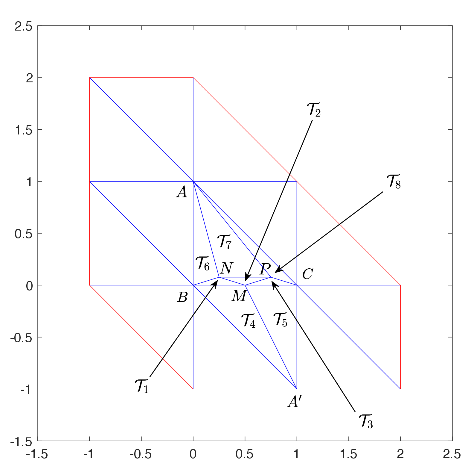
Figure 14: Patch \(E\) around triangle with degenerate mesh.
Lemma 8. The matrix \({{\mathbf{S}}}\) has the form \[\label{eq:smallstiffnessmat} {\mathbf{S}} = {\mathbf{E}}\widetilde{{\mathbf{S}}}{\mathbf{E}}^T,\tag{70}\] where \[\label{eq:smallstiffnessmatBR} {\mathbf{E}} = \begin{bmatrix}{\mathbf{I}}& -{\mathbf{R}}\\{\mathbf{0}}& {\mathbf{I}}\end{bmatrix},\;\mathrm{with}\; {\mathbf{R}} = {\mathbf{R}}_0 + {\mathbf{O}}(\alpha)\;\;\mathrm{and}\;\; {\mathbf{R}}_0 =\begin{bmatrix}1/2& 3/4& 1/4\\1/2& 1/4 & 3/4\\ 0& 0 & 0\end{bmatrix}.\tag{71}\]
Proof. Referring to Figures 10 and 14, note that \[\begin{align} \widetilde{\varphi}_B& =& {\varphi}_B + \widetilde{\varphi}_B(M) {\varphi}_M + \widetilde{\varphi}_B(N) {\varphi}_N + \widetilde{\varphi}_B(P) {\varphi}_P\\ & =& {\varphi}_B + \frac{1}{2} {\varphi}_M + \left(\frac{3}{4}+O(\alpha)\right) {\varphi}_N + \left(\frac{1}{4}+O(\alpha)\right) {\varphi}_P, \end{align}\] where we used the fact that \(N=N(\alpha) \to (1/4,0)\) as \(\alpha\to 0\), showing that \(\lim_{\alpha\to 0} \widetilde{\varphi}_B(N) = 3/4\). Due to the smoothness of the function \(\alpha\mapsto \widetilde{\varphi}_B(N(\alpha))\), we conclude that \(\widetilde{\varphi}_B(N) = 3/4 + O(\alpha)\). Similarly, \(\widetilde{\varphi}_B(P) = 1/4 + O(\alpha)\). Following the same line of arguments we have \[\begin{align} \widetilde{\varphi}_C& =& {\varphi}_C + \widetilde{\varphi}_C(M) {\varphi}_M + \widetilde{\varphi}_C(N) {\varphi}_N + \widetilde{\varphi}_C(P) {\varphi}_P\\ & =& {\varphi}_C + \frac{1}{2} {\varphi}_M + \left(\frac{1}{4}+O(\alpha)\right) {\varphi}_N + \left(\frac{3}{4}+O(\alpha)\right) {\varphi}_P, \end{align}\] and \[\begin{align} \widetilde{\varphi}_A& =& {\varphi}_A + \widetilde{\varphi}_A(M) {\varphi}_M + \widetilde{\varphi}_A(N) {\varphi}_N + \widetilde{\varphi}_A(P) {\varphi}_P\\ & =& {\varphi}_A + O(\alpha) {\varphi}_N + O(\alpha) {\varphi}_P. \end{align}\] If we redenote the basis functions (for the purpose of temporarily replacing the letter indices with numbers) \({{\mathcal{B}}} = \{{\psi}_i\}_{i=1,\dots,6}\) and \(\widetilde{{\mathcal{B}}} = \{\widetilde{\psi}_i\}_{i=1,\dots,6}\), then \[\begin{align} \psi_i = \sum_{j=1}^6 {\mathbf{E}}_{ij} \widetilde{\psi}_j,\;\;i=1,\dots,6,\;\;\mathrm{with} \end{align}\] \[\begin{align} {\mathbf{E}} = \begin{bmatrix} {}1{}& {}0{}& {}0{}& -\varphi_B(M)& -\varphi_B(N)& -\varphi_B(P)\\ 0& 1& 0& -\varphi_C(M)& -\varphi_C(N)& -\varphi_C(P)\\ 0& 0& 1& -\varphi_A(M)& -\varphi_A(N)& -\varphi_A(P)\\ 0& 0& 0& 1& 0& 0\\ 0& 0& 0& 0& 1& 0\\ 0& 0& 0& 0& 0& 1 \end{bmatrix} \end{align}\]
Therefore, \[\begin{align} {\mathbf{S}}_{ij} & =& a_E(\psi_j,\psi_i) = a_E\left(\sum_{k=1}^6{\mathbf{E}}_{jk}\widetilde{\psi}_k,\sum_{k=1}^6{\mathbf{E}}_{il}\widetilde{\psi}_l\right) =\sum_{k,l=1}^6{\mathbf{E}}_{jk} {\mathbf{E}}_{il}\: a_E\left(\widetilde{\psi}_k,\widetilde{\psi}_l\right)\\ & = & \sum_{k,l=1}^6{\mathbf{E}}_{jk} {\mathbf{E}}_{il} \widetilde{{\mathbf{S}}}_{lk} = \left({\mathbf{E}} \widetilde{{\mathbf{S}}}{\mathbf{E}}^T\right)_{ij}, \end{align}\] showing 70 . ◻
We can now proceed to prove of Theorem 9.
Proof. Using 70 we get \[\label{eq:smallstiffnessmatinv} {\mathbf{S}}^{-1} = {\mathbf{E}}^{-T}\widetilde{{\mathbf{S}}}^{-1}{\mathbf{E}}^{-1}.\tag{72}\] For computing \(\widetilde{{\mathbf{S}}}^{-1}\) we use the block inversion formula \[\label{eq:blockinverse} \widetilde{{\mathbf{S}}}^{-1} = \begin{bmatrix} {\mathbf{I}} & {\mathbf{0}} \\ {\mathbf{D}}^T & {\mathbf{I}} \end{bmatrix}\; \begin{bmatrix} {\widehat{{\mathbf{S}}}}^{-1} & {\mathbf{0}} \\ {\mathbf{0}} & {{\mathbf{C}}}^{-1} \end{bmatrix}\; \begin{bmatrix} {\mathbf{I}} & {\mathbf{D}} \\ {\mathbf{0}} & {\mathbf{I}} \end{bmatrix}\tag{73}\] with \(\widehat{{\mathbf{S}}} = {{\mathbf{A}}} - {{\mathbf{B}}} {{\mathbf{C}}}^{-1}{{\mathbf{B}}}^T\) being the Schur complement of \({{\mathbf{C}}}\), and \({\mathbf{D}} = -{{\mathbf{B}}}{{\mathbf{C}}}^{-1}\). Note that \(\alpha {\mathbf{C}} \approx {\mathbf{C}_0}\), hence \(\alpha^{-1}{\mathbf{C}}^{-1} \approx {\mathbf{C}_0}^{-1}\), showing that \[\begin{align} {\mathbf{C}}^{-1} = \alpha\left({\mathbf{C}_0}^{-1}+{\mathbf{O}}(\alpha)\right) = \alpha \left( \begin{bmatrix} 6 & 4 & 4\\ 4 & 7/2 & 5/2\\ 4 & 5/2 & 7/2 \end{bmatrix} +{\mathbf{O}}(\alpha)\right) . \end{align}\] Since \({\mathbf{B}} = {\mathbf{O}}(1)\) and \({\mathbf{C}}^{-1} = {\mathbf{O}}(\alpha)\), it follows that \[\begin{align} \widehat{{\mathbf{S}}} = {{\mathbf{A}}} - {{\mathbf{B}}} {{\mathbf{C}}}^{-1}{{\mathbf{B}}}^T = {{\mathbf{A}}} + {\mathbf{O}}(\alpha), \end{align}\] showing that \(\widehat{{\mathbf{S}}} \approx {{\mathbf{A}}}\). Hence, \[\begin{align} \label{eq:Ainv} \widehat{{\mathbf{S}}}^{-1} \approx {\mathbf{A}}^{-1} = \begin{bmatrix} 2/7 & 1/14 & 1/14\\ 1/14 & 15/56 & 1/56\\ 1/14 & 1/56 & 15/56 \end{bmatrix} > {\mathbf{0}}. \end{align}\tag{74}\] Therefore, using 73 we get \[\begin{align} \label{eq:blockinverseeplicit} &&\widetilde{{\mathbf{S}}}^{-1} = \begin{bmatrix} {\mathbf{I}} & {\mathbf{0}} \\ {\mathbf{D}}^T & {\mathbf{I}} \end{bmatrix}\; \begin{bmatrix} {\widehat{{\mathbf{S}}}}^{-1} & {\mathbf{0}} \\ {\mathbf{0}} & {{\mathbf{C}}}^{-1} \end{bmatrix}\; \begin{bmatrix} {\mathbf{I}} & {\mathbf{D}} \\ {\mathbf{0}} & {\mathbf{I}} \end{bmatrix} = \begin{bmatrix} {\widehat{{\mathbf{S}}}}^{-1} & {\widehat{{\mathbf{S}}}}^{-1}{\mathbf{D}} \\ {\mathbf{D}}^T {\widehat{{\mathbf{S}}}}^{-1} & {{\mathbf{C}}}^{-1} + {\mathbf{D}}^T {\widehat{{\mathbf{S}}}}^{-1}{\mathbf{D}} \end{bmatrix} \end{align}\tag{75}\] Note that \[\begin{align} {\mathbf{D}} &=& -{{\mathbf{B}}}{{\mathbf{C}}}^{-1} = -\alpha\begin{bmatrix} {1}/{2}& 0& 0\\{1}/{2}& 0& 0\\-{1}/{2}& 0& 0 \end{bmatrix} \left(\begin{bmatrix} 6 & 4 & 4\\ 4 & 7/2 & 5/2\\ 4 & 5/2 & 7/2 \end{bmatrix} +{\mathbf{O}}(\alpha)\right)\\ &=& \alpha \left(\begin{bmatrix} -3& -2& -2\\-3& -2& -2\\3& 2& 2 \end{bmatrix}+{\mathbf{O}}(\alpha)\right) = \alpha \left({\mathbf{D}}_0 + {\mathbf{O}}(\alpha)\right). \end{align}\] Therefore \[\begin{align} {{\mathbf{C}}}^{-1} + {\mathbf{D}}^T {\widehat{{\mathbf{S}}}}^{-1}{\mathbf{D}} = {\alpha}({\mathbf{C}}^{-1}_0+{\mathbf{O}}(\alpha)) + {\mathbf{O}}(\alpha^2) ={\alpha}({\mathbf{C}}^{-1}_0+{\mathbf{O}}(\alpha)). \end{align}\] Hence \[\begin{align} \label{eq:blockinverseeplicit2} &&\widetilde{{\mathbf{S}}}^{-1} = \begin{bmatrix} {{{\mathbf{A}}}}^{-1} + {\mathbf{O}}(\alpha) & \alpha {{{\mathbf{A}}}}^{-1}\left({\mathbf{D}}_0 + {\mathbf{O}}(\alpha)\right) \\ \alpha \left({\mathbf{D}}^T_0 + {\mathbf{O}}(\alpha)\right) {{{\mathbf{A}}}}^{-1} & {\alpha}({\mathbf{C}}^{-1}_0+{\mathbf{O}}(\alpha)) \end{bmatrix} \end{align}\tag{76}\] Putting together 71 , 72 , and 76 we get \[\begin{align} {\mathbf{S}}^{-1} &=& \begin{bmatrix} {{{\mathbf{A}}}}^{-1} & {{{\mathbf{A}}}}^{-1} {\mathbf{R}}_0\\ {\mathbf{R}}^T_0 {{\mathbf{A}}}^{-1}& {\mathbf{R}}^T_0 {{\mathbf{A}}}^{-1} {\mathbf{R}}_0 \end{bmatrix} +{\mathbf{O}}(\alpha) = {\mathbf{T}}_0 + {\mathbf{O}}(\alpha). \end{align}\] A direct computation shows that \[\begin{align} {\mathbf{A}}^{-1} {\mathbf{R}}_0 = \begin{bmatrix} 5/28 & 13/56 & 1/8\\ 19/112 & 27/224 & 7/32\\ 5/112& 13/224 & 1/32 \end{bmatrix} \end{align}\] and \[\begin{align} {\mathbf{R}}^T_0{\mathbf{A}}^{-1} {\mathbf{R}}_0 = \begin{bmatrix} 39/224 & 79/448 & 11/64\\ 79/448 & 183/896 & 19/128\\ 11/64 & 19/128 & 25/128 \end{bmatrix}, \end{align}\] showing, together with 74 , that \({\mathbf{T}}_0 >{\mathbf 0}\). Since \({\mathbf{S}}^{-1} = {\mathbf{T}}_0 +{\mathbf{O}}(\alpha)\), we have \[\lim_{\alpha\to 0} {\mathbf{S}}^{-1} = {\mathbf{T}}_0.\] Note that \({\mathbf{T}}_0\) is singular, and has rank 3, hence is rank-3 deficient. The computation has been validated numerically against stiffness matrix computations using standard finite element codes. ◻
We return to the proof of Lemma 7.
Proof. The fact that the \({{\mathbf{A}}}\) block has the form 68 is a simple consequence of the formulas 45 and 47 , and are well known for a uniform grid. Due to the fact \(\widetilde{\varphi}_A\), \(\widetilde{\varphi}_B\), \(\widetilde{\varphi}_C\) are linear on \(\Delta ABC\), and \(\varphi_N, \varphi_P\) vanish on \(\partial (\Delta ABC)\), we have \[\begin{align} a_E(\widetilde{\varphi}_X, \varphi_Y) = 0,\;\;\forall X \in \{A, B, C\},\;\; Y \in \{N, P\}. \end{align}\] (see also Lemma 5.5 in [17]), thus justifying all the six zero-entries in the matrix \({{\mathbf{B}}}\). The remaining non-trivial entries are associated with the set \(\{\varphi_M, \varphi_N, \varphi_P\}\).
Entries related to \({\varphi}_N, {\varphi}_P\): This case has been discussed in Lemma 5.6 in [17]; for completeness we review the computation, which is simplified because we are interested primarily in the case when \(0< \alpha \ll 1\). Refer to Figure 14 for notation. We have \[\begin{align} a_E(\varphi_N, \varphi_N) &= &\int_{{\mathcal{T}}_1\cup {\mathcal{T}}_2\cup {\mathcal{T}}_6\cup{\mathcal{T}}_7} |\nabla\varphi_N|^2 \\ &= &\frac{\sin(\pi-2 \alpha)}{2 \sin^2\alpha} + \frac{\sin\alpha}{2 \sin(\pi-2 \alpha) \sin\alpha} + \int_{{\mathcal{T}}_6\cup{\mathcal{T}}_7} |\nabla \varphi_N|^2\\ & = & \frac{\cos \alpha}{\sin\alpha} + \frac{1}{2 \sin(2 \alpha)} + O(1) = \frac{1}{\alpha}\left(\frac{5}{4} + O(\alpha) \right). \end{align}\] Similarly, \[\begin{align} a_E(\varphi_P, \varphi_P) &= & \frac{1}{\alpha}\left(\frac{5}{4} + O(\alpha) \right). \end{align}\] Furthermore, if \(\gamma\) denotes the angle \(\sphericalangle NAP\), then \[\begin{align} a_E(\varphi_N, \varphi_P)& = & -\frac{\sin(\gamma+\pi-2\alpha)}{2 \sin \gamma \sin(\pi-2\alpha)} = -\frac{\sin(2\alpha-\gamma)}{2 \sin \gamma \sin(2\alpha)} \\ &= & -\frac{\cos \gamma}{2 \sin \gamma} +\frac{\cos(2\alpha)}{2 \sin(2\alpha)} = \frac{1}{\alpha}\left(\frac{1}{4} + O(\alpha) \right) \end{align}\] because \(\lim_{\alpha\to 0} \gamma(\alpha) = \gamma_0\in (0,\pi/4)\), showing that the expression involving \(\gamma\) is bounded as \(\alpha\to 0\).
Entries related to \({\varphi}_M\): The quantities \(a_E(\varphi_M, \widetilde{\varphi}_X)\) with \(X \in \{A, B, C\}\) cannot be computed using 45 , because the latter are not nodal basis functions with respect to the finer mesh. First note that \(\nabla \widetilde{\varphi}_A = e_2\), showing that \[\begin{align} a_E(\varphi_M, \widetilde{\varphi}_A)& = & \int_{{\mathcal{T}}_1\cup {\mathcal{T}}_2\cup {\mathcal{T}}_3} \partial_y\varphi_M. \end{align}\] Let \(g:[0,1]\to E\) be the piecewise linear function whose graph is represented by the contour \(BNPC\). Using Fubini’s theorem and the fact that \(\varphi_M(g(x)) = 0\), we obtain \[\begin{align} \int_{{\mathcal{T}}_1\cup {\mathcal{T}}_2\cup {\mathcal{T}}_3} \partial_y\varphi_M & = & \int_0^1 dx \int_0^{g(x)}\partial_y\varphi_M(x,y) = - \int_0^1 \varphi_M(x,0) dx = -\frac{1}{2}, \end{align}\] because \(\varphi_M(x,0)\) is a one-dimensional, piecewise linear nodal basis function on \(\overline{BC}\). Therefore \(\widetilde{{S}}_{34} = \widetilde{{S}}_{43}=-1/2\). For similar reasons, if \(A'=(1,-1)\) denotes the vertex on \(\partial E\) directly below \(C\) (see Figure 14), and \(\widetilde{\varphi}_{A'}\) is the coarse nodal basis function associated with \(A'\), then \[\begin{align} a_E(\varphi_M, \widetilde{\varphi}_{A'}) &=& \int_{{\mathcal{T}}_4\cup {\mathcal{T}}_5} \nabla {\varphi}_{M} \cdot \nabla \widetilde{\varphi}_{A'} = -\frac{1}{2}. \end{align}\]
Since \(\mathrm{supp}(\varphi_M) = \bigcup_{i=1}^5 {\mathcal{T}}_i \subseteq\mathrm{supp}(\widetilde{\varphi}_B)\cap \mathrm{supp}(\widetilde{\varphi}_C)\), we have \[\begin{align} a_E(\varphi_M, \widetilde{\varphi}_X)& = & \int_{{\mathcal{T}}_1\cup\dots\cup {\mathcal{T}}_5} \nabla \varphi_M\cdot \nabla \widetilde{\varphi}_X,\;\;X\in \{B,C\}. \end{align}\] Note that on \(D_M^{(1)} = {\mathcal{T}}_1\cup {\mathcal{T}}_2 \cup {\mathcal{T}}_3\) we have \(\nabla \widetilde{\varphi}_C = e_1\), while on \(D_M^{(2)} = {\mathcal{T}}_4\cup {\mathcal{T}}_5\) we have \(\nabla \widetilde{\varphi}_B = -e_1\). Hence, after using Fubini’s theorem \[\begin{align} \label{eq:Dm1} &&\int_{D_M^{(1)}} \nabla \varphi_M \cdot \nabla \widetilde{\varphi}_C = \int_{D_M^{(1)}} \partial_x \varphi_M = \int_0^{\frac{1}{4}\tan \alpha } dy \int_{D_{M,y}^{(1)}} \partial_x \varphi_M \;dx = 0, \end{align}\tag{77}\] where \(D_{M,y}^{(1)}\) is the horizontal section of \(D_{M}^{(1)}\) at level \(y\), and we use the fact that \(\varphi_M\) is zero at the end points of each horizontal section of \(D_{M}^{(1)}\). Similarly, \[\begin{align} \label{eq:Dm2} && \int_{D_M^{(2)}} \nabla \varphi_M \cdot \nabla \widetilde{\varphi}_B = -\int_{D_M^{(2)}} \partial_x \varphi_M = -\int_{-1}^{0} dy \int_{D_{M,y}^{(2)}} \partial_x \varphi_M \; dx = 0, \end{align}\tag{78}\] for the same reason. It remains that \[\begin{align} \label{eq:MBC} && a_E(\varphi_M, \widetilde{\varphi}_B) = \int_{D_M^{(1)}} \nabla \varphi_M\cdot \nabla \widetilde{\varphi}_B,\;\;\; a_E(\varphi_M, \widetilde{\varphi}_C) = \int_{D_M^{(2)}} \nabla \varphi_M\cdot \nabla \widetilde{\varphi}_C. \end{align}\tag{79}\]
On \(\Delta ABC\) we have \(\widetilde{\varphi}_B + \widetilde{\varphi}_C + \widetilde{\varphi}_A \equiv 1\), thus (implicitly) this holds on \(D_M^{(1)}\). So \[\begin{align} 0 &= & \int_{D_M^{(1)}} \nabla \varphi_M \cdot \nabla (\widetilde{\varphi}_B + \widetilde{\varphi}_C + \widetilde{\varphi}_A) \stackrel{\eqref{eq:Dm1}}{=} \int_{D_M^{(1)}} \nabla \varphi_M \cdot \nabla \widetilde{\varphi}_B + \int_{D_M^{(1)}} \nabla \varphi_M \cdot \nabla \widetilde{\varphi}_A\\ & \stackrel{\eqref{eq:MBC}}{=} & a_E(\varphi_M, \widetilde{\varphi}_B) + a_E(\varphi_M, \widetilde{\varphi}_A), \end{align}\] showing that \[\begin{align} a_E(\varphi_M, \widetilde{\varphi}_B) = \frac{1}{2}. \end{align}\] On \(\Delta A'BC\) we have \(\widetilde{\varphi}_B + \widetilde{\varphi}_C + \widetilde{\varphi}_{A'} \equiv 1\), thus (implicitly) this holds on \(D_M^{(2)}\). So \[\begin{align} 0 &= & \int_{D_M^{(2)}} \nabla \varphi_M \cdot \nabla (\widetilde{\varphi}_B + \widetilde{\varphi}_C + \widetilde{\varphi}_{A'}) \stackrel{\eqref{eq:Dm2}}{=} \int_{D_M^{(2)}} \nabla \varphi_M \cdot \nabla \widetilde{\varphi}_C + \int_{D_M^{(2)}} \nabla \varphi_M \cdot \nabla \widetilde{\varphi}_{A'}\\ & \stackrel{\eqref{eq:MBC}}{=} & a_E(\varphi_M, \widetilde{\varphi}_C) + a_E(\varphi_M, \widetilde{\varphi}_{A'}), \end{align}\] showing that \[\begin{align} a_E(\varphi_M, \widetilde{\varphi}_C) = \frac{1}{2}, \end{align}\] as well. Therefore, \[\begin{align} && \widetilde{S}_{14} = \widetilde{{S}}_{41}= \widetilde{{S}}_{24} = \widetilde{{S}}_{42}=1/2, \end{align}\] which concludes the computation of the block \({{\mathbf{B}}}\) (recall that the other entries are \(0\)). All these results can also be obtained by classical trigonometric arguments. Furthermore, using the formulas 45 and 47 we obtain \[\begin{align} &&a_E(\varphi_M, \varphi_N) = a_E(\varphi_M, \varphi_P) = -\frac{\sin (2 \alpha)}{2 \sin^2\alpha}= -\frac{\cos \alpha }{ \sin\alpha} =-\frac{1}{\alpha} (1 + O(\alpha)). \end{align}\] The last entry needed is \[\begin{align} a_E(\varphi_M, \varphi_M) &=& \int_{{\mathcal{T}}_1\cup \dots \cup {\mathcal{T}}_5}|\nabla \varphi_M|^2 \\ &= & \frac{1}{\sin(\pi-2\alpha)} + \frac{\sin(\pi-2\alpha)}{2\sin^2 \alpha} + \overbrace{\int_{{\mathcal{T}}_4\cup {\mathcal{T}}_5}|\nabla \varphi_M|^2}^{O(1)}\\ &=& \frac{3}{2\alpha} (1+O(\alpha)), \end{align}\] which concludes the computation of \(\widetilde{{\mathbf{S}}}\). ◻
9 Limits of discrete Green’s functions on some degenerate meshes↩︎
In this section we revisit a class of two-dimensional, triangular meshes analyzed in Section 6 of [17], for which the \({\mathcal{P}}_1\)-finite element solution of the Poisson equation with homogeneous Dirichlet boundary conditions satisfies the DMP, while potentially violating the angle condition in many places. The main purpose here is to expose the behavior of the discrete Green’s function as the mesh becomes degenerate. The examples in this section are easier to analyze than the one in Theorem 9.
9.0.0.1 The case of a single interior node.
The simplest nontrivial example of a finite element mesh is that of a triangular domain \(D = \Delta ABC\) with a single vertex \(P\) in the interior. We choose \(P\) so that the triangle \(\Delta PBC\) is isosceles with base angles equal to \(\theta\), as shown in Fig. 15 (left), although this is not essential. With only one interior mesh vertex, the stiffness matrix is just the real number \[{\mathbf{A}}(\theta) = a_D(\varphi_P,\varphi_P) = \int_{D} |\nabla \varphi_P|^2,\] where \(\varphi_P\) is the nodal basis function associated with \(P\).
We are interested in the behavior of the discrete Green’s function as \(\theta\to 0\). Cf 47 , \[{\mathbf{A}}(\theta) \ge \int_{{\mathcal{T}}_1} |\nabla \varphi_P|^2 = \frac{\sin(\pi-2\theta)}{2\sin^2 \theta} = \frac{2\sin\theta\cos\theta}{2\sin^2 \theta} = \cot \theta.\] Hence, \[\label{eq:convAPzero} \lim_{\theta\to 0}({\mathbf{A}}(\theta))^{-1} \le \lim_{\theta\to 0}\tan \theta = 0.\tag{80}\] This shows that the discrete Green’s function, which is represented by a number, converges to the only singular \(1\times 1\) matrix, namely the number 0. Also note that the mass matrix of the mesh stays bounded as \(\theta\to 0\). Therefore, given a fixed right hand side \(f\) for the Poisson equation on \(D\) with the mesh described above, the finite element solution \(u(\theta)\) will converge to \(0\) as \(\theta \to 0\). We remark that the limiting mesh, shown Fig. 15 (right), is a valid triangulation of \(D\) with no interior nodes. Note that the Poisson problem with homogeneous Dirichlet boundary conditions can also be formulated on the associated finite element space, which contains only the function 0. Hence, the solution will be zero, which is consistent with the limit of the solutions \(u(\theta)\).
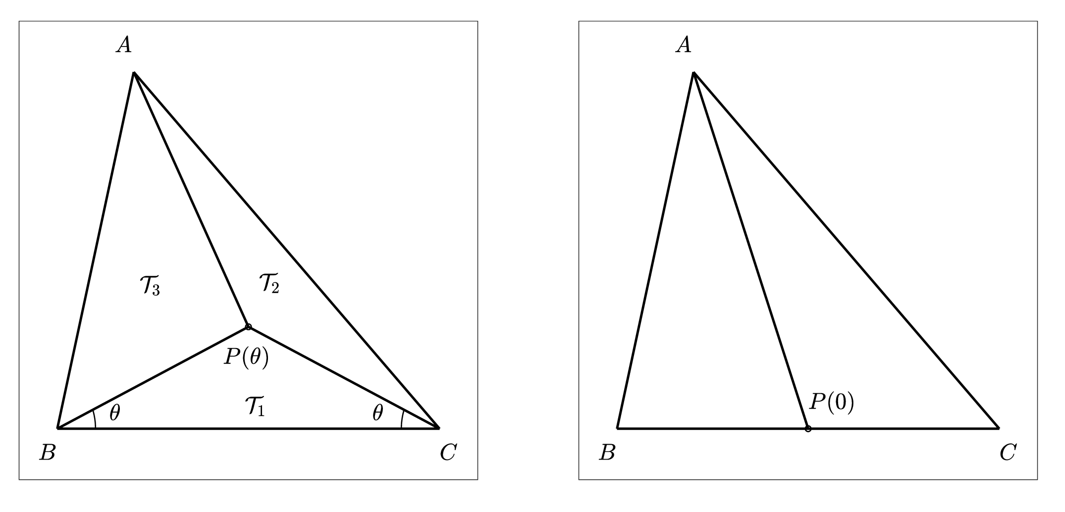
Figure 15: As \(\theta \to 0\) the mesh on the left converges to the mesh in the right image. When \(\Delta A B C\) is an interior triangle of another triangular mesh, the partition on the right will not be a valid mesh, since the triangle below \(\Delta A B C\) – not pictured – is not divided..
9.0.0.2 An embedded divided triangle.
For the second example consider a triangular mesh \({\mathcal{T}}_h\) on a polygonal domain \(D\), and we subdivide one interior triangle as in Fig. 15 (left), which results in a refined mesh \(\tilde{{\mathcal{T}}}_h = \tilde{{\mathcal{T}}}_h(\theta)\). If the discrete Green’s function is positive (or just nonnegative) on \({\mathcal{T}}_h\), it is shown in Section 6 of [17] that the same holds for \(\tilde{{\mathcal{T}}}_h\), regardless of the value of \(\theta>0\). For \(\theta = 0\), the subdivided triangle is shown in Fig. 15 (right). The resulting partition of \(D\) corresponding to \(\theta = 0\), with \(P(0)\) being the midpoint between \(B\) and \(C\), is not a valid triangulation, because the triangle in \({\mathcal{T}}_h\) below \(\Delta A B C\) is not subdivided. A similar invalid partition is depicted in [33], Fig. 3.12 (right), page 80.
The question we answer here is what happens to the discrete Green’s function on \(\tilde{{\mathcal{T}}}_h(\theta)\) as \(\theta\to 0\). We will describe this limit in terms of the discrete Green’s function on \({{\mathcal{T}}}_h\), and we show it is represented by a rank-1 deficient matrix. We denote by \({\mathcal{B}} = \{\varphi_1,\dots,\varphi_n\}\) the nodal basis associated with the interior vertices of \({\mathcal{T}}_h\), and let \({V}_0^h = \mathrm{span}({\mathcal{B}})\). Assume that \(\varphi_{n+1}\) is the nodal basis function in \(\tilde{{\mathcal{T}}}_h\) associated with \(P = P(\theta)\) (this was called \(\varphi_P\) from the previous example), and \(\varphi_{n-1}, \varphi_{n}\) correspond to \(B\) and \(C\), respectively. The set \(\tilde{{\mathcal{B}}} = {\mathcal{B}} \cup \{\varphi_{n+1}\}\) forms a hierarchical basis for the finite element space \(\tilde{V}_0^h\) on \(\tilde{{\mathcal{T}}}_h\). Cf. [17], we have \(a_D(\varphi_i,\varphi_{n+1}) = 0\) for \(i=1, \dots, n\), which leads to a decoupling of the linear system representing the Poisson equation when formulated in the hierarchical basis \(\tilde{{\mathcal{B}}}\). For \(f\in (\tilde{V}_0^h)^*\), the system reads: \[\label{eq:matpoisson} \begin{bmatrix} {\mathbf{A}} & 0\\ 0 & \alpha \end{bmatrix} \begin{bmatrix} {\mathbf{x}}\\ x_{n+1} \end{bmatrix} = \begin{bmatrix} {\mathbf{b}}\\ b_{n+1} \end{bmatrix},\tag{81}\] where \({\mathbf{A}}\) is the stiffness matrix of the problem in the basis \({\mathcal{B}}\) (hence on \(V_0^h\)), \(\alpha = a_D(\varphi_{n+1},\varphi_{n+1})\), with \({{\mathbf{b}}}\in \mathbb{R}^n\) given by \({{\mathbf{b}}}_i = \left< \varphi_{i} , f \right>\) for \(1\le i \le n\), and \(b_{n+1} = \left< \varphi_{n+1} , f \right>\). The solution of 81 is given by \[\label{eq:solpoisson} u = u(\theta) = \sum_{i=1}^{n+1} x_i \varphi_i,\;\;{\mathbf{x}} = {\mathbf{A}}^{-1} {\mathbf{b}},\;\;x_{n+1} = {b}_{n+1}/\alpha.\tag{82}\] If \(f\) is fixed and \(\theta \to 0\), it follows from 80 that \(x_{n+1} \to 0\). Hence, \[\label{eq:u0} u_0 = \lim_{\theta\to 0} u(\theta) = \sum_{i=1}^{n} x_i \varphi_i \in V_h^0.\tag{83}\] It follows that \[\label{eq:u0mean} u_0(P(0)) = \frac{1}{2}(u_0(B) + u_0(C)),\tag{84}\] showing that the limit as \(\theta\to 0\) of all the finite element solutions on \(\tilde{{\mathcal{T}}}\) lie in a subspace of co-dimension 1. In other words, the degenerate partition can be considered “harmless”, as the limiting solution \(u_0\) is simply the solution on the original mesh \({\mathcal{T}}_h\).
In order to describe the matrix representation \(\tilde{{\mathbf{G}}}(\theta)\) of the discrete Green’s function on \(\tilde{{\mathcal{T}}}\) and its limit as \(\theta\to 0\), we let \(f^{(i)}\) be the Dirac impulse forcing at the \(i^{\mathrm{th}}\) node, for \(i\le n\). Then in 82 we have \({\mathbf{b}}={\mathbf{e}}_i\) (\(i^{\mathrm{th}}\) unit vector), and \(b_{n+1} = 0\). Cf. 83 the limiting solution \(u_0^{(i)}\) lies in \(V_h^0\), and satisfies the same equation as the discrete Green’s function on \({\mathcal{T}}_h\). Hence, 84 implies that the vector representation of \(u_0^{(i)}\) in the basis \(\tilde{{\mathcal{B}}}\) is \[(\tilde{{\mathbf{g}}}^{(i)})^T = [({\mathbf{g}}^{(i)})^T, \frac{1}{2}({\mathbf{g}}^{(i)}_{n-1}+{\mathbf{g}}^{(i)}_{n})],\] where \({\mathbf{g}}^{(i)}\) is the \(i^{\mathrm{th}}\) column of the discrete Green’s function on \({\mathcal{T}}_h\).
If \(f^{(n+1)}\) is the Dirac impulse forcing at \(P(\theta)\), then the corresponding right-hand side in 82 satisfies, as \(\theta\to 0\) \[{\mathbf{b}}=\frac{1}{2}\left({\mathbf{e}}_{n-1} + {\mathbf{e}}_{n}\right),\;\;b_{n+1} = 1.\] By 83 , its vector representation is \[(\tilde{{\mathbf{g}}}^{(n+1)})^T = [\frac{1}{2}({\mathbf{g}}^{(n-1)}+{\mathbf{g}}^{(n)})^T, \frac{1}{2}({\mathbf{g}}^{(n)}_{n-1}+{\mathbf{g}}^{(n-1)}_{n})].\] Hence, if we denote by the matrix representation in \(\tilde{{\mathcal{B}}}\) of the limit of the discrete function as \(\theta\to 0\) is \[\tilde{{\mathbf{G}}}_0 = \lim_{\theta\to 0} \tilde{{\mathbf{G}}}(\theta) = \begin{bmatrix} {\mathbf{G}}& \overline{g}\\ \overline{{\mathbf{g}}}^T& \tilde{g}, \end{bmatrix} \in \mathbb{R}^{(n+1)\times (n+1)}.\] where \({\mathbf{G}}\) is the representation of the discrete Green’s function on the original mesh \({\mathcal{T}}_h\), and \[\overline{{\mathbf{g}}} = \frac{1}{2}({\mathbf{g}}^{(n-1)}+{\mathbf{g}}^{(n)}),\;\;\tilde{g} = \frac{1}{2}({\mathbf{g}}^{(n-1)}_{n-1}+{\mathbf{g}}^{(n)}_{n}).\] We used the equality \({\mathbf{g}}^{(n-1)}_{n} = {\mathbf{g}}^{(n)}_{n-1}\) to compute the last diagonal entry \(\tilde{g}\), which follows from the symmetry of the discrete Green’s function \({\mathbf{G}}\). Hence, the last column of \(\tilde{{\mathbf{G}}}_0\) is the average of the previous two, showing \(\tilde{{\mathbf{G}}}_0\) has rank \(n\). By contrast, the matrix \({\mathbf{T}}_0\) in Theorem 9 has rank-3 deficiency.
Acknowledgement↩︎
The authors sincerely thank the anonymous reviewers for their careful reading of the manuscript and for their valuable comments and constructive suggestions, which helped improve the quality of this work.
References↩︎
The first author was supported in part by NSF Award 2409951.↩︎