Uncertainty-Aware Ankle Exoskeleton Control
August 28, 2025
Abstract
Lower limb exoskeletons show promise to assist human movement, but their utility is limited by controllers designed for discrete, predefined actions in controlled environments, restricting their real-world applicability. We present an uncertainty-aware control framework that enables ankle exoskeletons to operate safely across diverse scenarios by automatically disengaging when encountering unfamiliar movements. Our approach uses an uncertainty estimator to classify movements as similar (in-distribution) or different (out-of-distribution) relative to actions in the training set. We evaluated three architectures (model ensembles, autoencoders, and generative adversarial networks) on an offline dataset and tested the strongest performing architecture (ensemble of gait phase estimators) online. The online test demonstrated the ability of our uncertainty estimator to turn assistance on and off as the user transitioned between in-distribution and out-of-distribution tasks (F1: 89.3). This new framework provides a path for exoskeletons to safely and autonomously support human movement in unstructured, everyday environments.
Exoskeletons, uncertainty-awareness, deep learning, rehabilitation robotics, anomaly detection.
1 Introduction↩︎
Lower limb exoskeletons are used in a variety of applications to increase human mobility, from assistance to rehabilitation [1]–[3]. Recent results from human-in-the-loop optimization experiment have highlighted their potential to augment energy economy or user preferences during walking, running, and stair climbing, among many other tasks [4]–[9]. These results, however, can be contrasted with the continuing rarity of lower limb exoskeletons in the real world, particularly for populations who could most use assistance across a broad range of activities of daily living, but for whom safety is a necessity. For these potential users, the control laws that define when and how much assistance the exoskeleton provides must be predictable and robust.
Most exoskeleton controllers are designed and optimized for a few cyclic actions such as steady-state walking and jogging, climbing stairs, and other repetitive movements [10]. This does not encompass the wide array of motions that people can perform in their daily lives. To address the limitations of steady-state controllers, data-driven controllers, especially deep learning-based controllers that handle temporal data, have shown promise in adjusting to various speeds and actions with adaptable torque control [11]–[20]. Recently, deep learning biological torque controllers have represented a major step towards task-agnostic control [21]. However, these learned controllers have the major problem of faulty actuation based on out-of-distribution data; that is, if the model receives data that is faulty (e.g., dropped sensor) or outside of its training distribution, it will still make a prediction and the exoskeleton will act, without knowing whether the prediction was accurate. Critically, if the user is performing an action that the model was never trained on (whether gait phase, biological torque, or anything else), the prediction is very likely to be poor.
When exoskeletons actuate in the wrong direction or at the wrong time, the consequences can be disastrous for safety and trust in the exoskeleton. This may be most important at the ankle when the foot is suspended above the ground, as actuating during these times may cause tripping. If assistance is unexpectedly removed from 2-5% of steps, user trust in the system has been shown to decrease [22]. Measures of exoskeleton trust are still being defined by the research community, but the harmful effect of failed assistance on trust, biomechanics, and safety can be assumed to be exacerbated in the presence of a wider variety of walking speeds, additional tasks, and transitions between task-specific controllers. There may also be more detriment to false positives than false negatives, in which the exoskeleton mistakenly actuates instead of turning off [23].

A naive solution to the issue of unknown actions is to collect a training dataset consisting of all possible actions and label whether each task is assistable; however, due to the vastness of possible human actions, this is unlikely to be achievable. Another proposed solution is to develop machine learning controllers that can generalize well enough beyond the training set to provide useful assistance in new actions. There has been limited success in this endeavor. Phase-based controllers can extrapolate to different speeds of walking and different inclines, but have not been shown to generalize to new activities. The biological torque control approach taken by Molinaro, Scherpereel et al. demonstrates some ability to generalize to unseen activities [21], largely maintaining the correct direction of torque, but accuracy dropped as low as \(R^{2}\)=0.24 for extremely dynamic tasks outside of its training set.
Without an all-encompassing training set or a perfectly generalizing controller, the safest thing for an exoskeleton to do when encountering an unknown movement or a movement the controller is not trained for may be to turn off. To do this, however, the controller must be aware of whether the movement is unknown or novel to the controller. We propose running an uncertainty estimator – in parallel with existing exoskeleton controllers – to determine whether an action is known (in-distribution) or unknown (out-of-distribution), and ultimately to decide whether to activate the exoskeleton controller or to turn off (Fig. 1).
Contrary to the task classification strategies used in exoskeletons to date, our proposed uncertainty-aware control approach employs a one-class classifier; it is designed only using examples from the in-distribution class and must determine if the new samples are significantly different. Due to the high dimensionality of the input data, which consists of both sensor and time dimensions, deep learning-based methods are necessary. Deep learning-based uncertainty awareness (similarly novelty detection or anomaly detection) has been widely studied in recent years across a variety of fields, including healthcare monitoring, manufacturing processes, and detecting fraud and fault, among others [24], [25]. For these purposes, deep learning is commonly used, especially for multivariate data [26]–[28]. In estimating the uncertainty of neural networks specifically, state-of-the-art applications used methods like reinforcement learning and Bayesian belief networks [29], [30]. This uncertainty awareness has been expanded to robot navigation and collision avoidance for reinforcement learning-based policies that can be used in real time [31]. In addition to mathematical models, autoencoders, GANs, and ensembles of models have been proposed and found some success as architectures for anomaly detection [26], [32]–[34]. Within biomechanics and assistive devices, Zhu et al. used deep learning-based anomaly detection to monitor the performance of wearable sensors in a prosthetic socket [35]. Hobbs et al. used a PCA based method to identify outliers in synthetic gait data based on EMG sensors and kinematic data, but it is not a real-time method and is not generalizable to actions beyond walking [36]. To our knowledge, our method is the first deep learning uncertainty estimator to make real-time decisions about wearable robotic assistance.
The primary contributions of this work include 1) a foundational exploration of estimating uncertainty across tasks in human movement, 2) comparison of three methods with high potential in this domain, and 3) the first real-time validation of an uncertainty-aware safety framework on an actuated lower limb exoskeleton in outdoor environments. Each uncertainty-aware model was trained on an n=9 training set of exoskeleton sensor data consisting of people walking and jogging on a treadmill (various inclines). The models were tuned on an n=3 offline validation set, and tested on a new set of in- and out-of-distribution data. The best performing model was then tested online on an outdoor circuit with n=3 new users. Our results demonstrate the feasibility of an uncertainty-aware exoskeleton controller for improved safety on unknown tasks. This approach offers a practical alternative to developing task-specific controllers for every possible movement—a currently intractable challenge that has hindered the real-world implementation of exoskeletons.
2 Human Movement Data for Model Training and Development↩︎
Two different datasets were used for the development of the models: 1) a training dataset \(D_{\text{train}}^{\text{ID}}\), which is in-distribution by definition, and 2) an offline validation dataset \(D_{\text{val}}^{\text{ID, OOD}}\)consisting of both in-distribution and out-of-distribution actions. All subjects provided informed consent, and this study was approved by the Northeastern Institutional Review Board.
The training dataset \(D_{\text{train}}^{\text{ID}}\)included 9 participants wearing ankle exoskeletons (EB60; Dephy Inc, Boxborough, MA) walking at various speeds and jogging at different inclines, previously presented in Shetty et al. [37]. Each task was performed under two conditions: actuated (using a simple Time-Based Estimator controller) and unactuated. Sensors include IMUs and ankle encoders on each boot. Ankle velocity was also calculated from ankle angle via finite differencing and included as a channel. Data were post-processed into overlapping time windows consisting of 175 samples, or approximately 1 s (using every tenth window). It was previously found that the gait phase model accuracy did not substantially improve when using more windows [37].
All actions were performed on a Force-Instrumented Treadmill (Bertec), which allowed us to calculate ground truth values for gait phase. Gait phase is used in our base controller: it is converted to a commanded exoskeleton torque via a spline, with spline parameters dependent on the predicted walking/jogging speed and ramp incline [37]. During the online validation (section V), this phase-based controller serves as a base controller for in-distribution movements.
The offline validation data \(D_{\text{val}}^{\text{ID, OOD}}\)was collected in the Northeastern motion capture laboratory with 3 subjects (1 subject from the training set, 2 new participants). It consists of a range of both in-distribution and out-of-distribution activities. Activities included:
In-distribution: overground and treadmill walking and jogging (actuated and unactuated)
Out-of-distribution: stationary postures, chair-based movements, standing exercises, jumping, backward walking, etc).
\(D_{\text{val}}^{\text{ID, OOD}}\)was prepared in the same manner as \(D_{\text{train}}^{\text{ID}}\). \(D_{\text{val}}^{\text{ID, OOD}}\)was not used in model training, though it was used to evaluate the models as we developed them. A separate offline test dataset \(D_{\text{test (offline)}}^{\text{ID, OOD}}\)was collected similarly to \(D_{\text{val}}^{\text{ID, OOD}}\)on 3 new participants, with some new tasks added, including incline and decline walking, lying down, new sitting activities, standing poses, etc. This dataset was completely withheld from the model development process, and was only used for our final offline evaluation of the models.
3 Uncertainty Estimation Models↩︎
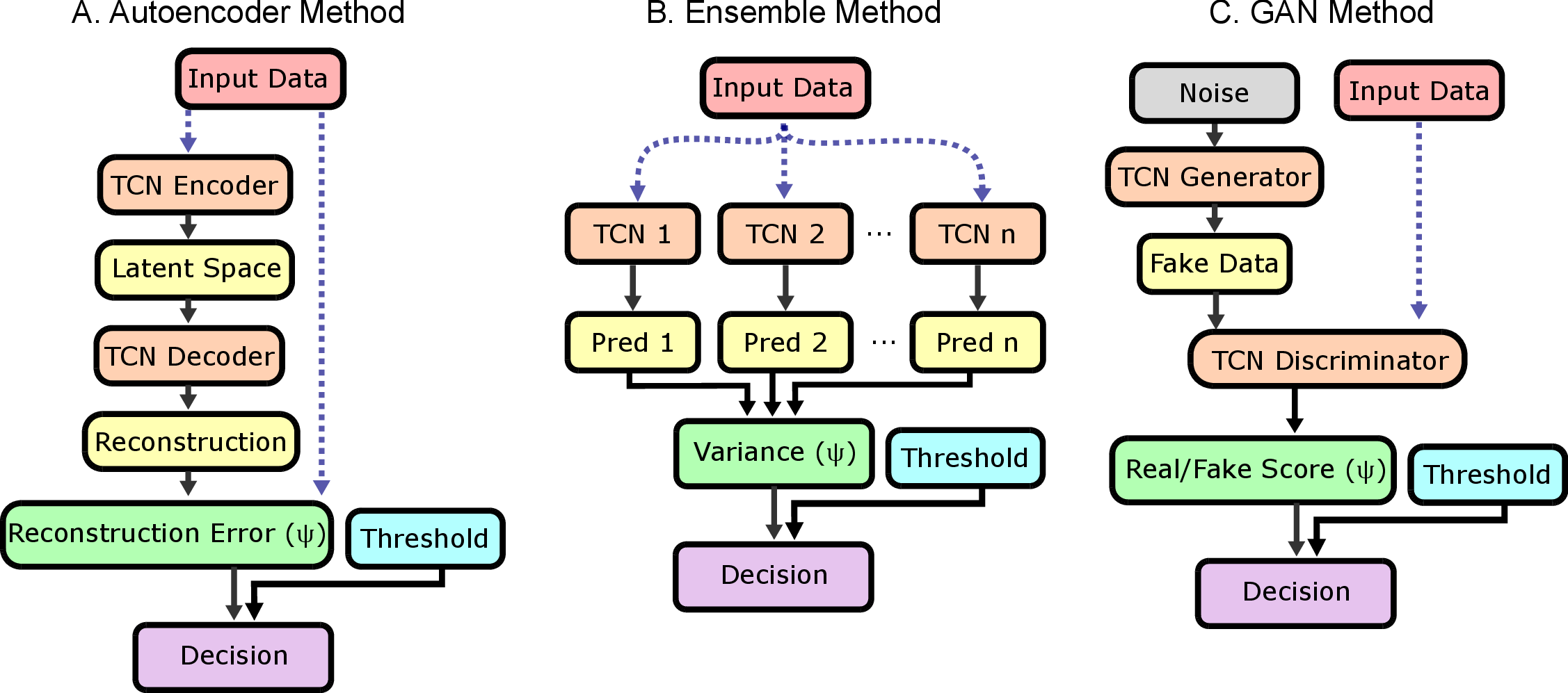
For uncertainty estimation, we focused on deep learning techniques, since our data is high-dimensional, multivariate, and temporal. All models used Temporal Convolutional Networks (TCNs) in their first layers due to their effectiveness in previous exoskeleton research [37]–[39]. TCNs use dilated causal convolutions that can be expressed as: \[F(s) = (x *_d f)(s) = \sum_{i=0}^{k-1} f(i) \cdot x(s-d \cdot i),\] where \(x\) is the input sequence, \(f\) is the filter, \(k\) is the filter size, and \(d\) is the dilation factor. Fig. 2 illustrates the three uncertainty classifier architectures implemented in this study, all of which employed TCNs.
3.1 Ensemble Method↩︎
Model ensembling is an established anomaly detection technique that leverages the differences between multiple similar models to detect anomalies in data [34]. We hypothesized that if multiple TCN models were trained on in-distribution data (e.g., starting from different initializations or training on different subsets of the data), their predictions would agree when presented with new sensor data that is similar to the training set but diverge when encountering unfamiliar sensor data. Thus, increased variance between model outputs would indicate out-of-distribution actions.
Our ensemble approach consists of 7 TCN models, each predicting the sine of gait phase for both the left and right leg [15]. We found that including more than 7 models did not further improve performance. To avoid the discontinuity at heel strike when gait phase switches from 100 percent to 0 percent, we predict the sine of gait phase similar to Kang et al. [40]. Each model \(i\) in the ensemble had two heads: one head predicts the sine of the gait phase for the left leg, \(l_i\), and the other head predicts that for the right leg, \(r_i\). At each timestep, for input data \(\mathbf{x}\), the uncertainty estimate \(\Psi\) is computed as the average of the variance of predictions across the left, \(l_1,\ldots, l_7\) and right legs, \(r_1,\ldots, r_7\), \[\Psi(\mathbf{x}) = (Var(l_1,\ldots, l_7) + Var(r_1,\ldots, r_7))/2.\] The hyperparameters of the TCN were taken from the gait phase model in previous work [37]. The models were trained with one subject withheld as the early stopping subject. This subject was rotated through the 9 subjects to find the average number of epochs before the models overfit. The final model was then trained for this number of epochs with all subjects included.
The ensemble method as described so far has a disadvantage of requiring a ground truth label for its prediction variable–in this case gait phase, which already existed in our previously collected training data. Similar to other possible labels used in exoskeleton control, such as biological joint torque, gait phase can be costly to collect and process (and may require extra sensing). Furthermore, gait phase is not well-defined for non-cyclic tasks, meaning that in-distribution training data can only be cyclic actions like walking and running. This makes it less generalizable to future implementations that include a non-cyclic action in their in-distribution set.
An alternate strategy could be to create a synthetic target that generalizes to a broader set of actions in the in-distribution test set. We explored several simple targets (e.g., means of channels, weighted polynomial combinations of channel means, etc). We found positive results for a synthetic target consisting of the sum of all correlations between all sensor channels across the window of input data. Thus, we similarly tested TCNs trained to predict these correlations (instead of sine of gait phase), and our results will distinguish between “Ensemble Method (Gait Phase)” and “Ensemble Method (Synthetic Target).”
3.2 Autoencoder↩︎
To eliminate the dependence on labels, we explored autoencoder architectures, which are widely used for anomaly detection on time series data and require only unlabeled data [24], [28], [41]–[43]. Our autoencoder architecture employs a TCN-based encoder and decoder, and attempts to reconstruct the input data itself:
\[\mathbf{z} = f_{\text{enc}}(\mathbf{x}), \quad \hat{\mathbf{x}} = f_{\text{dec}}(\mathbf{z})\]
Autoencoders create a bottleneck in an intermediate layer, forcing the network to learn a compressed representation of the training data. Typically, reconstruction error (\(x - \hat{x}\)) is used as the uncertainty score, since out-of-distribution data is less likely to reconstruct well. However, as described in the offline results (Section 4.3), reconstruction error did not work well as an uncertainty score for our application, likely because \(D_{\text{val}}^{\text{OOD}}\)contains a significant amount of low-complexity stationary data, such as standing, which is particularly easy for the model to reconstruct.
Instead, we focus on the latent representation, which captures essential features of the training data. We hypothesized that in-distribution data will cluster in the latent space, with anomalous data falling outside these regions. Therefore, we used Local Outlier Factor (LOF) on the latent space. LOF is an unsupervised anomaly-detection technique that works well in low-dimensional problems; it evaluates the local density of each sample relative to its neighbors:
\[\Psi(\mathbf{x}) = -\text{LOF}_k(\mathbf{z})\] The initial parameters chosen for the autoencoder were drawn from TCNs used in previous work, with the dominant hyperparameters associated with latent space size explored further in Section 4.3 [37].
3.3 Generative Adversarial Network (GAN)↩︎
The final architecture we explored as a plausible approach to our uncertainty detection problem is Generative Adversarial Networks (GANs). GANs are an adversarial training approach consisting of a generator \(G\) and a discriminator \(D\). The advantage that GANs provide comes from their ability to model data distributions. Namely, GANs attempt to directly model the data distribution of all in-distribution tasks, as well as directly classify them as in-distribution or out-of-distribution (on a continuous scale from 0 - 1), instead of using reconstruction variability and accuracy as an intermediary.
Specifically, the generator model within the GAN learns to turn noisy inputs into outputs that mimic our in-distribution data. The discriminator learns to determine when it receives real in-distribution data and when it receives fabricated data from the discriminator. By directly modeling in-distribution data and utilizing noise, GANs offer the possibility to capture more complex patterns and directly make a decision boundary between in-distribution and out-of-distribution data while only training on in-distribution data.
Our GAN’s generator utilizes a TCN-based decoder and the discriminator utilizes a TCN-based encoder. Together, the GAN trains with the standard adversarial loss: \[\min_G \max_D \mathcal{L}_{\text{GAN}}(G, D) = \mathbb{E}_{\mathbf{x}}[\log D(\mathbf{x})] + \mathbb{E}_{\mathbf{z}}[\log(1 - D(G(\mathbf{z})))]\] After training, the generator should successfully mock in-distribution data and the discriminator works as a binary classifier for in-distribution and out-of-distribution. For our uncertainty measure, we directly use the discriminator output. This output is a value between 0 and 1 on how confident the discriminator is about classifying the input. We use this as an uncertainty measure so that we can provide a threshold that is more tailored to our dataset.
\[\Psi(\mathbf{x}) = 1 - D(\mathbf{x})\]
This approach has the advantage of being able to learn complex patterns but is often unstable in training [44]. This approach was the most difficult to tune due to the interactive nature between the generator and the discriminator in the GAN. Adversarial models do not use a downward trending loss as a measure of improvement over training epochs, as a decrease in generator loss is often paired with an increase in discriminator loss, and vice versa. Additionally, it is vital that the generator and discriminator both improve at a rate in which neither overpower the other, as an overpowered discriminator will yield poor gradients to the discriminator and an overpowered generator will lead to mode collapse, as this typically means the generator is learning to output certain specific styles of output, rather than model the in-distribution data distribution.
There exist a variety of approaches to help improve and stabilize GANs. Certain approaches that we tried include gradient clipping, utilizing the generator to produce our uncertainty measure, or incorporating a reconstruction metric to evaluate the extent to which the generator would modify in-distribution data. The parameters chosen for the GAN were mostly determined by testing and monitoring the relative strength between the generator and the discriminator. As the discriminator is classifying rather than creating realistic data, it often overpowered the generator. To account for this, we weaken the discriminator by utilizing the spectral norm, updating it fewer times and with a smaller learning rate than the generator.
4 Offline Testing↩︎
4.1 Training↩︎
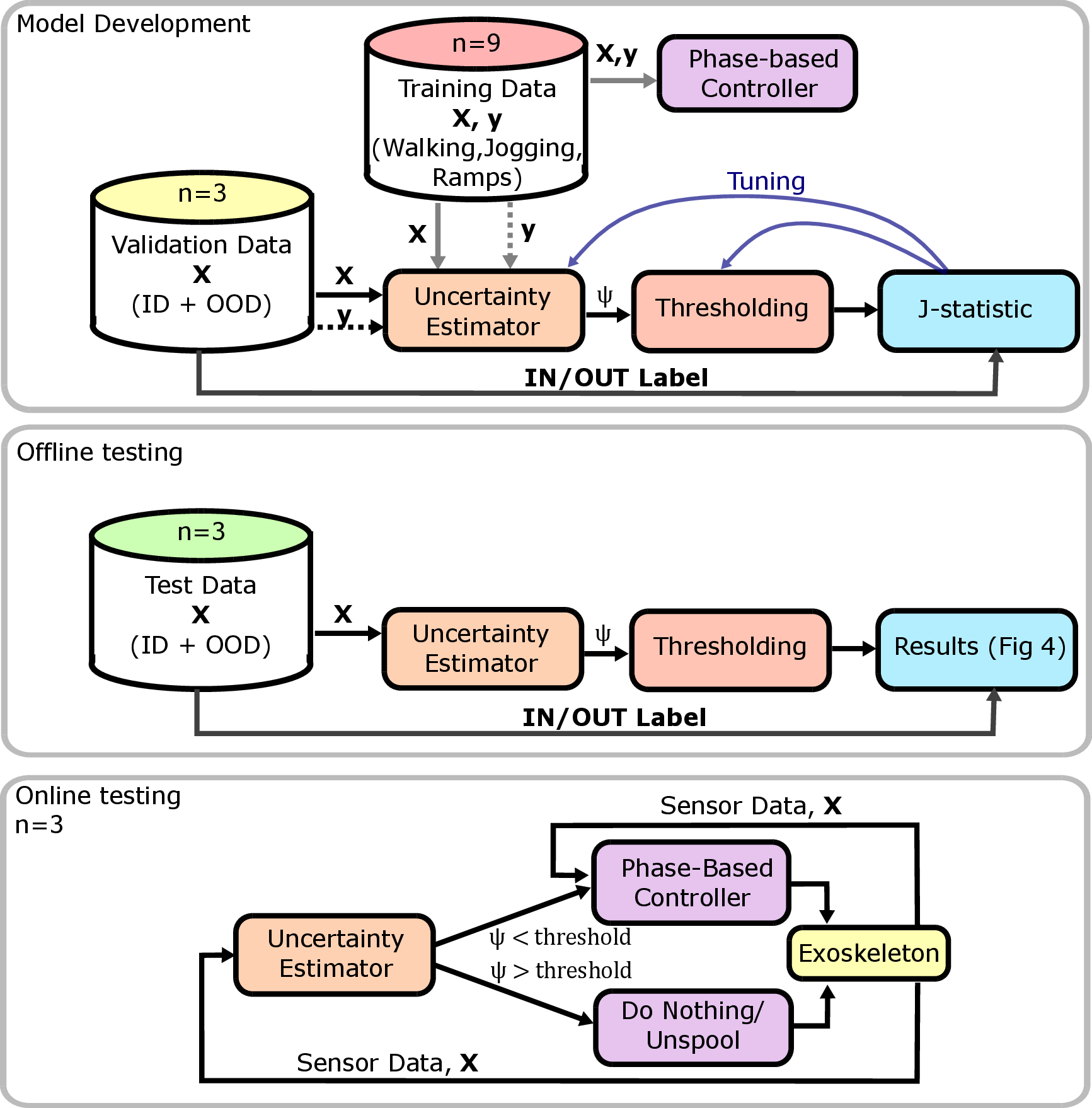
All the models tested were trained only on the in-distribution training set \(D_{\text{train}}^{\text{ID}}\). This is crucial for our end objective of creating a framework that future researchers can use for their desired in-distribution tasks, and which does not require additional collection of out-of-distribution tasks since they can never be entirely representative of human movement. However, preliminary model development required us to use a validation set consisting of both in-distribution and out-of-distribution data (\(D_{\text{val}}^{\text{ID, OOD}}\))
Compared to typical data-driven techniques in exoskeleton control, there are increased difficulties in designing and testing uncertainty-detection models without overfitting. First, model development and hyperparameter tuning requires testing on an offline dataset that consists of both in-distribution and out-of-distribution data. Ideally, the out-of-distribution task set is long enough to allow for a subset of tasks to be withheld for final testing, such that the model is not overfit to the specific tasks chosen in the validation set. To achieve this, we collected two offline datasets, a validation set (\(D_{\text{val}}^{\text{ID, OOD}}\)) and a test set (\(D_{\text{test (offline)}}^{\text{ID, OOD}}\)). \(D_{\text{val}}^{\text{ID, OOD}}\)included 3 subjects, 1 of which was in the training dataset \(D_{\text{train}}^{\text{ID}}\), while 2 were novel. It consisted of a set of in- and out-of-distribution tasks. \(D_{\text{test (offline)}}^{\text{ID, OOD}}\)consisted of an additional 3 novel subjects, and included tasks from \(D_{\text{val}}^{\text{ID, OOD}}\)in addition to new in- and out-of-distribution tasks.
For model development, models were trained on \(D_{\text{train}}^{\text{ID}}\)and then run on \(D_{\text{val}}^{\text{ID, OOD}}\), where their performance and J-statistic was observed to make decisions about architecture changes and hyperparameter tuning, and threshold heuristic selection. \(D_{\text{test (offline)}}^{\text{ID, OOD}}\)was completely withheld from this process. Once the models had achieved satisfactory performance on \(D_{\text{val}}^{\text{ID, OOD}}\), they were run on \(D_{\text{test (offline)}}^{\text{ID, OOD}}\)to obtain the offline results detailed in Section 4.3. The best performing model was also run on \(D_{\text{test (online)}}^{\text{ID, OOD}}\), which consisted of an additional 3 novel subjects on a continuous outdoor course detailed in Section 5. This training, model development, and testing process is shown in Fig 3.
In addition to hyperparameter tuning, the performance of uncertainty classification is highly sensitive to the uncertainty threshold, which controls the balance between the false positive and false negative rates. A threshold could be derived from \(D_{\text{test (offline)}}^{\text{ID, OOD}}\)to optimally balance these false positive and negatives; however, we considered our findings to be more powerful if we fixed the threshold using only training data \(D_{\text{train}}^{\text{ID}}\). In the best case scenario, this would enable other researchers to implement our methods without needing to collect out-of-distribution samples, and expect the method to work out-of-the-box. We set the threshold as the value that contained 99.5 percent of the uncertainty scores when using only \(D_{\text{train}}^{\text{ID}}\), which we considered to represent a reasonable (0.5%) fixed false negative rate. Notably, fixing the threshold in this manner may cause the threshold to be highly dependent on a few outlier movements in the training set.
For all models, an 88 point (\(\sim\)0.5s) causal median filter was applied to the uncertainty scores. The vast majority of the frequency content of human movements is below \(\sim\)10 Hz [45]; filtering the output removes spikes in the predictions that do not represent true transitions between in- and out-of-distribution tasks. However, increasing the filter strength comes with added delay, causing poor performance during task transitions. We assume our 0.5 s median filter to add 0.25 s delay during transitions.
4.2 Evaluation↩︎
Performance was assessed using standard metrics: accuracy, recall, precision, F1-score, and J-statistic [46]. Youden’s J-statistic (0-100%) is defined as: \[\text{J-statistic} = \text{Recall} + \text{Specificity} - 1,\] where recall represents the proportion of actual out-of-distribution instances correctly identified, and specificity represents the proportion of in-distribution instances correctly identified. We used the J-statistic in addition to the other standard metrics because it is more robust to heavy class imbalances, which are common in anomaly detection tasks and in our test sets [47]. \(D_{\text{test (offline)}}^{\text{ID, OOD}}\)consisted of 80.1% out-of-distribution windows, while \(D_{\text{test (online)}}^{\text{ID, OOD}}\)consisted of 57.1% out-of-distribution windows. Fig 4 demonstrates the model performance on various task groups in \(D_{\text{test (offline)}}^{\text{ID, OOD}}\)to further clarify the model’s performance on this dataset.
To assess the quality of probabilistic predictions, we also evaluated calibration using Expected Calibration Error (ECE) and Brier score. ECE measures the average absolute difference between predicted probabilities and actual frequencies across confidence bins [48], with lower values indicating better calibration. Brier score quantifies the mean squared difference between predicted probabilities and true outcomes [49], where a score of 0 represents perfect calibration and 0.25 is equivalent to always predicting 0.5. For models that output unbounded anomaly scores (ensemble variance and LOF scores), we converted these to calibrated probabilities using sigmoid transformation [50]: \(p = 1/(1 + \exp(-s(\text{score} - \text{threshold})))\), where \(s\) is a steepness parameter and the threshold centers the sigmoid at \(p=0.5\). The steepness parameter was optimized using leave-one-subject-out cross-validation to minimize Brier score, ensuring no subject-level data leakage in calibration parameter selection. For the GAN discriminator, which already outputs probabilities via its sigmoid activation, we used the discriminator output directly without recalibration. We report calibration metrics using the pre-set training-based threshold (99.5th percentile of training uncertainty scores) in Table 1.
To compare the effect of threshold choice, we also calculated the ECE and Brier score using using a threshold post-hoc optimized from \(D_{\text{test (offline)}}^{\text{ID, OOD}}\). Threshold choice showed varying impact on calibration across architectures: minimal effect for the gait phase ensemble (\(<\)6% change in both metrics), substantial improvement for the synthetic target ensemble (39% and 32% reductions in Brier and ECE, respectively), moderate improvement for the LOF autoencoder (16% and 5% reductions), and no change for the GAN discriminator as expected from its direct probability outputs. To further evaluate the model robustness to threshold choice, we calculated the area under the ROC curve as well as the J-statistic of the model using both thresholds, reported in Fig. 4 [51].
To evaluate our proposed uncertainty classification approaches, we conducted offline testing across all architectures using \(D_{\text{test (offline)}}^{\text{ID, OOD}}\). The models are run in the following steps:
Pass a window (175 samples, or \(\sim\)1 second) of scaled data into the pre-trained model and get the uncertainty score for this window.
Filter the output with an 88 point (\(\sim\)0.5s) causal median filter.
Label the window as in or out-of-distribution based on whether the filtered uncertainty score is above or below the threshold.
Mark the window as correct if the label of the window is the same as the ground truth label of the window.
Calculate the overall accuracy, precision, recall, F1 score, J-statistic, ECE, and Brier score.
4.3 Offline Results↩︎
| Method | Accuracy (%) | Precision (%) | Recall (%) | F1-Score (%) | J-Statistic (%) | ECE | Brier |
|---|---|---|---|---|---|---|---|
| Ensemble Method (Gait Phase) | 96.1 \(\pm\) 1.3 | 93.0 \(\pm\) 5.6 | 96.2 \(\pm\) 2.8 | 90.3 \(\pm\) 3.8 | 92.3 \(\pm\) 3.5 | 0.03 | 0.03 |
| Ensemble Method (Synthetic Target) | 76.9 \(\pm\) 2.6 | 45.7 \(\pm\) 4.7 | 99.4 \(\pm\) 0.8 | 62.5 \(\pm\) 4.6 | 70.9 \(\pm\) 3.3 | 0.22 | 0.13 |
| Autoencoder | 69.8 \(\pm\) 10.9 | 40.0 \(\pm\) 12.2 | 94.7 \(\pm\) 6.1 | 55.7 \(\pm\) 12.8 | 58.5 \(\pm\) 16.9 | 0.26 | 0.18 |
| GAN | 89.4 \(\pm\) 2.7 | 74.9 \(\pm\) 13.0 | 68.7 \(\pm\) 3.8 | 71.5 \(\pm\) 7.8 | 63.0 \(\pm\) 6.5 | 0.06 | 0.09 |
Values are reported as mean \(\pm\) standard deviation across three subjects in the offline test set.
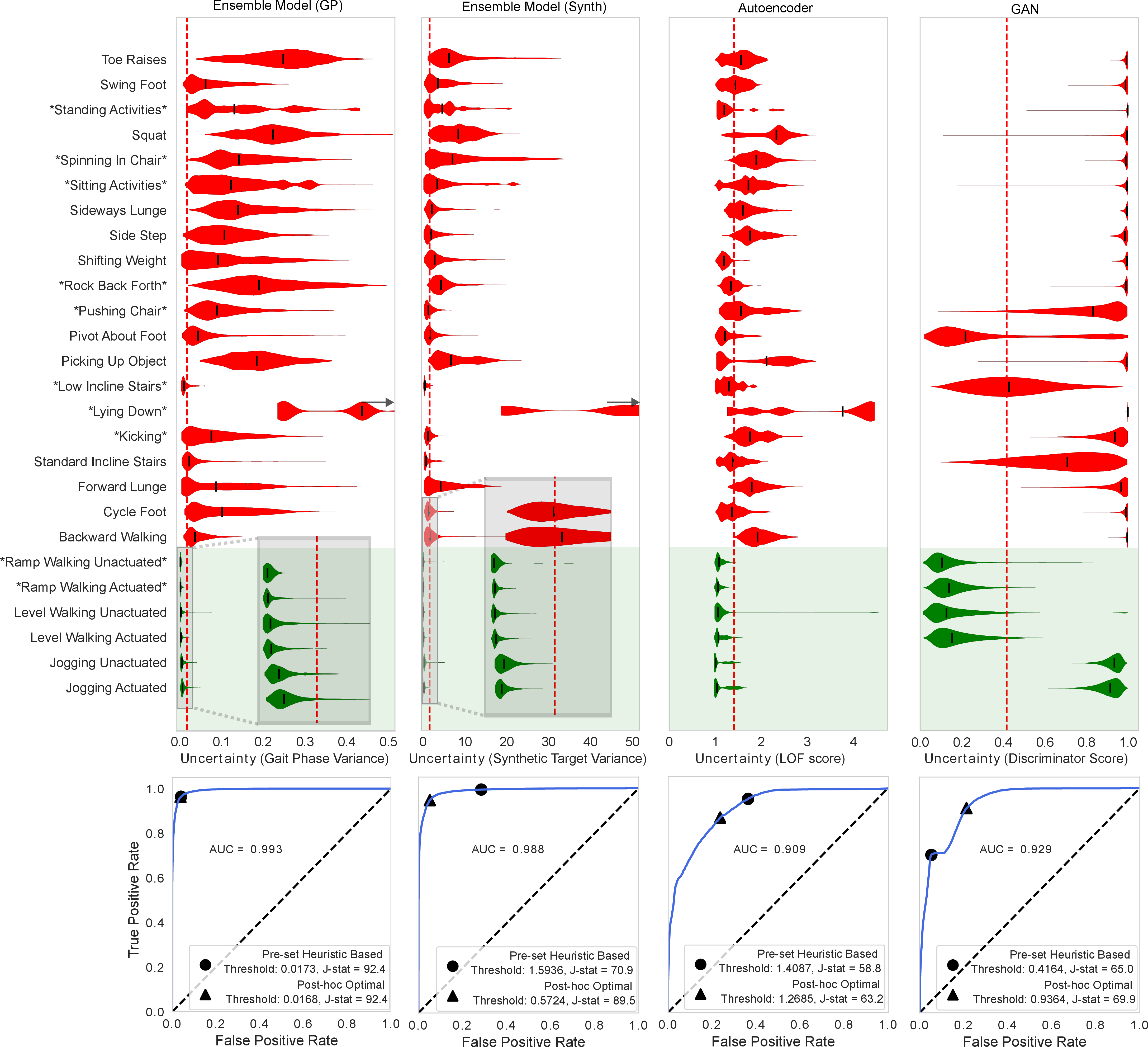
The gait phase ensemble method demonstrated strong performance on \(D_{\text{test (offline)}}^{\text{ID, OOD}}\)(J: 92.3, AUROC: 0.993). The gait phase ensemble sometimes misidentified stair ascent and descent (both cyclic tasks), especially on low incline stairs, as well as forward lunge, kicking, and shifting weight. Table 1 presents the performance metrics for each method, and Fig 4 shows each model’s performance by task.
The synthetic target ensemble model performed poorly compared to the gait phase ensemble model in our evaluation framework (J: 70.9). However, the in-distribution and out-of-distribution predictions did maintain good separability, obtaining a J-statistic of 89.5 when using a threshold post-hoc optimized from \(D_{\text{test (offline)}}^{\text{ID, OOD}}\), and the AUROC was 0.988. This method demonstrates a promising direction for future research to allow ensemble methods to move away from gait phase labels.
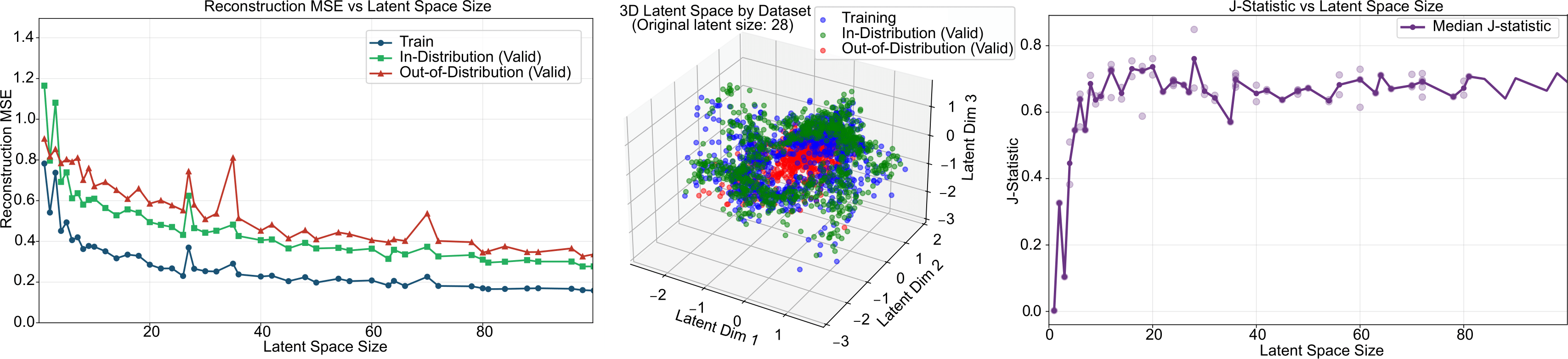
The autoencoder is not reliant on a gait phase label, but performed worse than both ensemble methods (J: 58.5, AUROC: 0.909). We performed a brute-force sweep of latent space dimensions to better understand the effect of latent space size (Fig. 5). We hypothesized that for a small latent space, the model would poorly reconstruct both in- and out-of-distribution data, leading to poor separability. For large latent spaces, the autoencoder would learn to pass the input sequence through with minimal compression leading to easy reconstruction for both in- and out-of-distribution data. At an optimally sized latent space, we hypothesized that the autoencoder would compress input data enough that the model would be able to reconstruct in-distribution data well but not out-of-distribution data, leading to a separable uncertainty score of reconstruction error. However, after observing the performance of models across our latent space size sweep, the \(D_{\text{val}}^{\text{OOD}}\)reconstruction was not significantly separated from \(D_{\text{val}}^{\text{ID}}\)at any latent space size, and \(D_{\text{val}}^{\text{ID}}\)consistently reconstructed worse than \(D_{\text{train}}^{\text{ID}}\)(Fig. 5). We hypothesize that the good reconstruction of \(D_{\text{val}}^{\text{OOD}}\)is due to many of our out-of-distribution actions being stationary—i.e., sitting, standing, performing exercises in place, etc. This is easy for an autoencoder to reconstruct, even without prior data, as little to no movement can be approximated as a 0 for each channel.
The latent representations for \(D_{\text{val}}^{\text{ID}}\)and \(D_{\text{val}}^{\text{OOD}}\)were more separable, with in-distribution data exhibiting a ring-like structure often seen in cyclic data (Fig. 5). To take advantage of this better separation in the latent space than in the reconstruction error, we used Local Outlier Factor on the latent space as our uncertainty score, so a new window would be evaluated on how far its latent space representation fell outside of the distribution of the latent space of the training data. Using this method, we were able to obtain a model with a J-statistic of 84.9 on \(D_{\text{val}}^{\text{ID, OOD}}\). However, these results were not generalizable to \(D_{\text{test (offline)}}^{\text{ID, OOD}}\), with the model obtaining a J-statistic of 58.5.
The GAN-based approach is not reliant on a gait phase label, and demonstrated good performance in labeling many out-of-distribution actions correctly. However, it labeled jogging as out-of-distribution despite it being well-represented in \(D_{\text{train}}^{\text{ID}}\), hurting its overall performance (J: 63.0, AUROC: 0.929). In addition, its performance was highly sensitive to the hyperparameters chosen; thus the GAN may have been more likely than the other architectures to be overfit to \(D_{\text{val}}^{\text{ID, OOD}}\), and its performance may not be generalizable to other actions. This hypothesis is somewhat supported by the GAN’s worst performing out-of-distribution tasks in \(D_{\text{test (offline)}}^{\text{ID, OOD}}\), many of which are tasks that were not included in \(D_{\text{val}}^{\text{ID, OOD}}\).
The ensemble of gait phase models performed the highest on \(D_{\text{test (offline)}}^{\text{ID, OOD}}\), was the least sensitive to hyperparameters, and had the lowest and least variable ECE and Brier score, therefore we selected it for online implementation and further testing.
5 Online Model Testing↩︎
Testing models online is critical to demonstrating control approaches are viable. Because the exoskeleton is actuated (or sometimes unactuated), and the user’s biomechanics are altered by assistance, the incoming sensor readings depend on the controller output. This feedback loop typically causes degraded performance relative to offline testing, and can even cause instabilities if implementation is poor. In addition, our online test consisted of three novel subjects and a range of new tasks that were not included in \(D_{\text{val}}^{\text{OOD}}\)or \(D_{\text{test (offline)}}^{\text{OOD}}\), providing an unbiased estimate of model performance across unseen tasks.
5.1 Online Implementation↩︎
For online and real-time evaluation, our implementation architecture consisted of three components implemented similarly to previous work, with the addition of our uncertainty estimator running in parallel with the gait phase estimator [37]:
Dephy ExoBoot Hardware: Ankle exoskeleton equipped with IMUs and encoders that provide raw sensor data and execute torque commands.
Jetson Orin Nano: Executes the model inference of both Uncertainty Estimator (Gait Phase Ensemble Model) and Gait Phase predictor.
Raspberry Pi: Receives sensor data from the Exoboots, performs basic processing and communications, and sends torque commands. It serves as the intermediary between the Jetson and the exoskeleton hardware.
The model developed and tested offline was converted from a pytorch model to a TRT for more efficient online performance on the Jetson. The end-to-end system operates at 105 Hz.
5.2 Online Experiment Methods↩︎
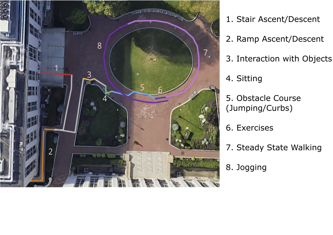
We designed a test route around Northeastern University campus (Fig. 6) that included various terrains and actions to validate the system’s performance in real-world conditions:
Stair station: Ascending and descending stairs.
Ramps and suspension station: Ascending and descending a ramp, and hanging with participant’s feet off of the ground.
Object interaction station: Picking up and throwing away an item in a trashcan that opens with a foot pedal, and picking up objects off the ground.
Sitting station: Transitioning between sitting and standing, sitting on a bench, tapping feet while sitting, and moving positions while sitting.
Obstacle course station: Jumping and walking on and off of the curb, and skipping.
Plyometrics station: Squats, lunges, toe raises, jumping jacks (subject 1 only).
Steady state walking: Walking around the course at a brisk pace.
Jogging: Jogging around the course at a slow pace.
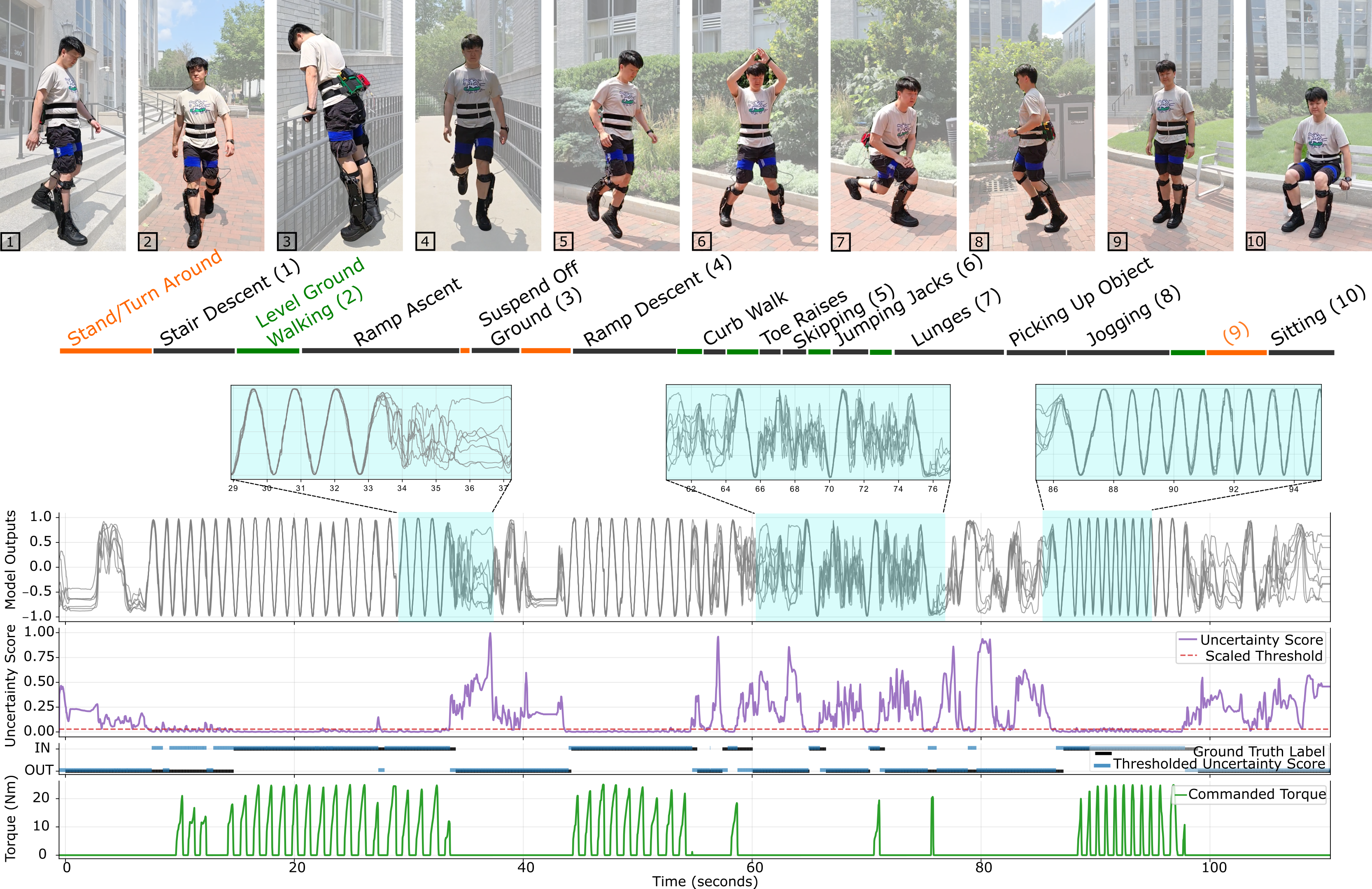
Three novel subjects performed this circuit with the ensemble of gait phase estimators providing real-time uncertainty estimates (Fig. 7). When the uncertainty score was below the threshold (predicting in-distribution), the phase-based exoskeleton controller was active and providing torque. When out-of-distribution, the exoboot actuators unspooled, providing zero impedance. The model outputs and applied torque were recorded, as well as video footage of the participant traversing the obstacle course, which was time-synced to the model outputs for later evaluation. For subjects 2 and 3, jumping jacks were removed from the circuit due to hardware issues on high impact tasks. To generate ground truth labels for evaluation, we employed three external observers (not on the research team) to mark timestamps in the video recordings where they would judge an activity to be in-distribution (\(D_{\text{test (online)}}^{\text{ID}}\)) or out-of-distribution (\(D_{\text{test (online)}}^{\text{OOD}}\)). Labelers were instructed to label a timestamp as in-distribution if the subject was walking or jogging for two or more steps, and label everything else as out-of-distribution. The ground truth label (as a function of time) was then defined by majority voting from the labelers. The online evaluation metrics were calculated by comparing model classifications against these ground truth labels.
5.3 Online Results↩︎
| Dataset | Accuracy (%) | Precision (%) | Recall (%) | F1-Score | J-Statistic |
|---|---|---|---|---|---|
| Transitions vs Steady State | |||||
| Transition (entire dataset) | 65.5 \(\pm\) 7.8 | 69.4 \(\pm\) 5.4 | 49.4 \(\pm\) 21.6 | 55.8 \(\pm\) 17.0 | 30.1 \(\pm\) 15.6 |
| Steady State (entire dataset) | 89.1 \(\pm\) 1.8 | 89.4 \(\pm\) 3.6 | 92.3 \(\pm\) 2.1 | 90.8 \(\pm\) 1.2 | 77.0 \(\pm\) 4.7 |
| Transition (No stair section) | 62.7 \(\pm\) 8.9 | 71.4 \(\pm\) 6.6 | 48.1 \(\pm\) 24.4 | 54.4 \(\pm\) 19.8 | 26.6 \(\pm\) 16.4 |
| Steady State (No stair section) | 92.4 \(\pm\) 1.8 | 96.3 \(\pm\) 1.0 | 92.3 \(\pm\) 2.1 | 94.2 \(\pm\) 1.2 | 84.7 \(\pm\) 3.8 |
| Overall | |||||
| All Actions Total | 87.6 \(\pm\) 1.6 | 88.6 \(\pm\) 3.1 | 90.1 \(\pm\) 2.6 | 89.3 \(\pm\) 1.0 | 74.4 \(\pm\) 4.0 |
| All Actions Except Stairs Total | 90.4 \(\pm\) 1.9 | 95.2 \(\pm\) 0.3 | 90.1 \(\pm\) 2.6 | 92.5 \(\pm\) 1.4 | 81.0 \(\pm\) 3.3 |
Values are reported as mean \(\pm\) standard deviation across three subjects in the outdoor test set.
The time-course of the uncertainty score and individual model outputs are shown in Fig. 7. The overall F-1 score and J-statistics for the online model in the novel circuit were 89.3% and 74.4%, a decrease from the performance on the offline dataset where the F-1 score was 90.3% and the J-statistic was 92.3% (Table 2). The overall AUROC for the online testing was 0.818 \(\pm\) 0.20, also a decrease from the offline AUROC of 0.993. All sections had accuracies above 85% except for the stair section which had an accuracy of 71.1% (Table 3–Note that we report model performance by action group as accuracy, since each group is either fully in- or fully out-of-distribution). With the stair section removed, the model F-1 score and J-statistic improved to 92.5% and 81.0%, respectively.
After observing that the first subject’s performance on the stairs was significantly worse than the rest of the sections, we collected online data of the remaining subjects ascending and descending a separate set of stairs. The stairs on the outdoor course had a lower incline than standard stairs, with a rise of 15 cm and a run of 41 cm. The separate set of stairs we collected fell within the standard dimensions of indoor stairs, with a rise of 18 cm and a run of 28.5 cm. The model’s average online accuracy on these standard stairs was 88.9%. Similar results can be seen in the model performance offline, as shown in Fig. 4 where the model misclassified the low incline stairs much more than the standard stairs.
To further characterize the model’s online performance, we defined transition regions as the reviewer-labeled timestamps for transitions between in/out-of-distribution \(\pm\) 0.5s. These regions do not have an easy definition of in- vs out-of-distribution. We observed that the transition regions performed significantly worse than the non-transition regions; removing the transitions increased the F-1 score and J-statistic to 90.8% and 77.0% including stairs, and 94.2% and 84.7% without stairs.
6 Discussion↩︎
This study demonstrates a novel uncertainty estimator for use in lower limb exoskeletons, allowing differentiation between in-distribution and out-of-distribution actions. Our test of the uncertainty estimator running in parallel with an ML-based gait phase estimator demonstrates how the uncertainty estimator can be implemented online in tandem with other actuation control algorithms that are designed for specific actions, but fail for others. The uncertainty estimator is shown to work online with actuation on novel subjects in a diverse outdoor environment on a multitude of different actions including but not limited to plyometrics, sitting, walking on ramps, interacting with objects, and walking on and off multi-level surfaces like curbs. The model achieved an F1 score of 94.2% and a J-stat of 84.7% (not counting transitions and stairs) on novel subjects.
| Section/Action Group | Accuracy (%) |
|---|---|
| Level Ground Walking | 89.4 \(\pm\) 3.1 |
| Incline and Decline Walking | 96.7 \(\pm\) 2.9 |
| Jogging | 86.5 \(\pm\) 6.0 |
| Stairs | 71.1 \(\pm\) 13.3 |
| Slow Out of Distribution Tasks | 90.7 \(\pm\) 1.6 |
| Fast Out of Distribution Tasks | 86.7 \(\pm\) 5.4 |
Values are reported as mean \(\pm\) standard deviation across three subjects in the outdoor test set.
The largest decreases in performance came from the stair incline and decline portion of the course. As demonstrated in Fig 4 and the online performance on the separate set of standard stairs, the model performed much better on standard stairs both online and offline than it did on the low incline stairs. The flatter, wider steps that were a part of our course likely provided less of a distinction from ramps, causing the model to falsely label much of the stair ascent and descent as in-distribution and hurting the overall accuracy of the model. We suggest including both stairs and ramps with similar inclines into the same grouping in future implementations.
The offline test set did not include any transitions between in- and out-of-distribution actions, so some decrease in performance can be attributed to the addition of these transitions. Transitions can be difficult or impossible to define categorically, as they may be somewhere between in and out-of-distribution and there is no definitive moment of transition. In addition, the TCN has a window of 1 second of previous data that it uses to make its prediction for the current sample, so when a user has just transitioned to an out-of-distribution action, some of that window is still from the time when they were conducting an in-distribution action (and vice versa). Future implementations of this algorithm should include a gradual and smooth scaling of torque when transitioning between in-distribution and out-of-distribution movements.
Even with some shortcomings in our current uncertainty estimator, it adds safety to the base controller, since the actions that are most distinct from the training data (e.g., jumping) have the fewest false positives (Fig. 4). For tasks that are clearly out-of-distribution, like standing still or jumping in the air, the uncertainty estimator performs very well. This can have the effect of preventing actuation at especially consequential moments like when the foot is off the ground, as demonstrated during the jumping tasks and during a task where the participant suspended their feet off the ground by leaning on a railing. Moreover, falsely actuating on tasks that are out of distribution but biomechanically similar to those in the training dataset is less likely to be safety critical, as the exoskeleton controller may still provide useful assistance. Future work should improve uncertainty estimator performance to better handle out-of-distribution tasks that are close to in-distribution tasks.
The model was only trained on \(D_{\text{train}}^{\text{ID}}\), which was collected with IMUs, encoders, and force plates (only needed for the ensemble of gait phase estimators). Our offline validation set \(D_{\text{val}}^{\text{ID, OOD}}\)was used for model development and hyperparameter tuning, with the ensemble of gait phase estimators being the only model to achieve high enough performance on \(D_{\text{test (offline)}}^{\text{ID, OOD}}\)to try online. The online implementation only requires the onboard exoskeleton IMUs and encoders, allowing it to be implemented in any location or environment. Future work could see attempting this same method on other exoskeletons to see how much or little this method needs to be changed to achieve similar results with other datasets. In addition, for the ensemble of gait phase TCNs, the validation set was only used for evaluating the model before testing it offline and online, not in the construction of the model or its parameters (that is, it worked well “out of the box"). If others were to implement a similar method for their own exoskeletons using cyclic data, a validation set may not be needed.
Our approach allows for wider use of existing exoskeleton controllers in different environments and on different actions. Many exoskeleton controllers have been designed specifically for a discrete set of tasks. Researchers have largely ignored how their controllers will perform outside of these tasks; for instance, time-based estimator and even gait-phase estimators are likely to provide unhelpful “assistance” when the user is doing non-cyclic tasks, or even cyclic tasks that are far from the intended use case such as skipping or walking backwards. Similarly, controllers based on neuromechanical models often rely on the user performing tasks where reflexes are active, or ignore antagonist muscles that may co-contract during highly dynamic movements [52], [53]. Our concept of a high-level “actuate” vs. “do-not-actuate” classifier, designed via uncertainty estimation, can be layered on top of these controllers, with the goal of enabling the devices to be used safely outside of their designed task set. We anticipate that this will open up possibilities for many researchers to safely take their exoskeletons out of the lab and facilitate real-world implementation.
Future directions include pursuing a version of this estimator that is not reliant on gait phase, as this limits the in-distribution action set to those with a definable gait phase. The ensemble of models trained to predict the synthetic target can generalize to different training sets, and in the semi-supervised case with the tuned threshold, the performance was nearly equivalent; it is possible that future work in designing a synthetic target and/or defining the threshold could match the gait phase ensemble’s performance. The autoencoder and GAN approaches were difficult to tune, and the GAN was particularly sensitive to the chosen hyperparameters. Future work can continue to refine these approaches. While there are many potential avenues of continued development and refinement, this study overall represents a promising first step into the use of real-time uncertainty estimators for exoskeleton control in unknown situations, enabling the safe use of deep learning based task-agnostic control strategies.
7 Conclusion↩︎
This study successfully developed and validated an uncertainty-aware control framework enabling ankle exoskeletons to safely operate beyond controlled laboratory settings. Our ensemble of gait phase estimators achieved robust real-time uncertainty estimation, allowing seamless switching between specialized controllers and safe operational modes during diverse real-world activities. This framework represents a significant advancement toward practically implementable exoskeletons that can provide context-aware assistance across everyday environments while maintaining critical safety standards during unanticipated movements.
| Parameter | Value/Description |
|---|---|
| Common Data Preparation (All Models) | |
| Subjects | S02-S10 (9 subjects) |
| Trials | T01, T02, T04-T12 (11 trials) |
| Window size | 175 samples (1 second at 175 Hz) |
| Input channels | 16 (bilateral sensor data) |
| Input features | accel_[x,y,z], gyro_[x,y,z], ankle_angle, ankle_velocity \(\times\) 2 |
| Scaling | StandardScaler (pre-trained) |
| Smoothing | SMA (88 samples, 0.5 second window) |
| Ensemble Models | |
| Architecture | Multi-branch convolutional predictor, 7 branches, 3 layers/branch |
| Filters/Kernel | 30 filters/layer, kernel size 20 |
| Activation/Norm | ReLU, BatchNorm1d after each convolution |
| Training params | Step: 10, Batch: 1024, LR: 0.001, Optimizer: Adam |
| Loss function | MSE |
| Early stopping | 10 epochs patience during LOSO; final model uses LOSO-determined epochs |
| Anomaly scoring | Variance across 7 branch predictions, 99.5th percentile threshold |
| Ensemble: Gait Phase Model | |
| Target | Physiological gait phase signals, dual outputs (left/right) |
| Output/Loss | Tanh activation (range \([-1, 1]\)), MSE loss, Final epochs: 13\(^1\) |
| Ensemble: Synthetic Target Model | |
| Target | Correlation-based: \(\sum_{i>j} \text{corr}(x_i, x_j)\), single output |
| Output/Loss | Linear activation, MSE loss, Final epochs: 34\(^1\) |
| Autoencoder Model | |
| Architecture | Conv. autoencoder with temporal compression |
| Encoder/Decoder | Conv1d(16→19→24→bottleneck), kernel sizes: 15, 17, 19; Mirror decoder |
| Compression | Time dimension of latent space: 7, Filter dimension of latent space: 4, Latent space size: 28 |
| Activation/Norm | ReLU, BatchNorm1d after each layer, No dropout |
| Training params | Step: 10, Batch: 1024, LR: 0.001*(1024/16), Optimizer: Adam |
| Loss function | MSE |
| Early stopping | 80/20 train/valid split, patience=5 |
| Anomaly scoring | LOF(latent space), 99.5th percentile threshold |
| GAN Model | |
| Generator | ConvTranspose1d(10→10→12→16), kernel: 3, LeakyReLU(0.2) |
| Discriminator | Conv1d(16→30→30) w/ spectral norm, kernel: 5, ReLU, dropout: 0.2 |
| Output/Latent | Sigmoid (discriminator), Latent: 10 channels \(\times\) 35 time steps |
| Training params | Step: 20, Batch: 256, LR: G=2e-4, D=5e-5, Exp. decay (\(\gamma\)=0.99) |
| Optimizer/Loss | Adam (\(\beta\)=(0.5, 0.999)), Binary Cross-Entropy |
| Training | 500 epochs (fixed), 80/20 split, 5 G updates per 1 D update |
| Checkpointing | Every 5 epochs |
| Anomaly scoring | Discriminator output D(x), 99.5th percentile threshold |
| Training Strategy Comparison | |
| Ensemble | Stage 1: LOSO validation, Stage 2: Train on all subjects |
| AE/GAN | Single stage: Train on all subjects with validation split |
VIII. Appendix
References↩︎
*These authors contributed equally to this work.↩︎
This work was supported in part by U.S. National Science Foundation FRR Award under Grant 2328050 and Grant 2328051 and in part by Northeastern University’s Research Computing team. (Corresponding author: Fatima Mumtaza Tourk.) This work involved human subjects or animals in its research. Approval of all ethical and experimental procedures and protocols was granted by Northeastern Institutional Review Board, #22-11-29, and performed in line with the Declaration of Helsinki.
F. M. Tourk is with the Department of Mechanical Engineering, Northeastern University, Boston, MA 02115 USA (e-mail: tourk.f@northeastern.edu).
B. Galoaa is with the College of Engineering, Northeastern University, Boston, MA 02115 USA.
S. Shajan is with the Khoury College of Computer Sciences, Northeastern University, Boston, MA 02115 USA.
M. Everett is with the Department of Electrical & Computer Engineering, Khoury College of Computer Sciences, and the Institute for Experiential Robotics, Northeastern University, Boston, MA 02115 USA.
A. J. Young is with the Woodruff School of Mechanical Engineering and the Institute for Robotics and Intelligent Machines, Georgia Institute of Technology, Atlanta, GA 30332-0405 USA.
M. K. Shepherd is with the Department of Mechanical Engineering, the Department of Physical Therapy, Movement, and Rehabilitation Science, and the Institute for Experiential Robotics, Northeastern University, Boston, MA 02115 USA.↩︎