Stability of the Active Flux Method in the Framework of Summation-by-Parts Operators
July 15, 2025
Abstract
The Active Flux method is a numerical method for conservation laws using a combination of cell averages and point values, based on ideas from finite volumes and finite differences. This unusual mix has been shown to work well in many situations. We expand the theoretical justifications of the Active Flux method by analyzing it from the point of view of summation-by-parts (SBP) operators, which are routinely used to analyze finite difference, finite volume, and finite element schemes. We show that the Active Flux method can be formulated using degenerate SBP operators, yielding a first and novel approach for showing the energy stability of the Active Flux method.
Active Flux method, summation-by-parts operators, conservation laws, finite difference methods, finite volume methods
AMS subject classification. 65M06, 65M20, 65M70
1 Introduction↩︎
The Active Flux schemes are a recently developed class of methods introduced to solve systems of hyperbolic conservation laws (see [1]–[3]). They combine two types of degrees of freedom: cell averages and shared point values at the cell interfaces. The Active Flux method uses a globally continuous approximation, which is conceptually different to other finite volume methods. Yet, the conservative updates of the cell averages resemble a finite volume method and are given by the fluxes through the boundary of the cell. The Active Flux method approximates these fluxes by quadratures directly using the point values. This is in contrast to many finite volume schemes that use Riemann solvers to define the fluxes.
Two ways how the point values can be updated in time have emerged. Initially (e.g., in [3], [4]), it was proposed to use a short-time (approximate) solution of the initial-value problem (IVP) of the conservation law. Such an approach is appropriate for many equations (see [2], [5] for scalar conservation laws and for hyperbolic systems of conservation laws in one spatial dimension) and the resulting method is a one-stage method. The solution of the IVP naturally includes upwinding which is helpful for stability upon explicit integration in time. Since it is quite challenging to find short-time (approximate) third-order accurate solutions for multi-dimensional systems of conservation laws, it was proposed in [6], [7] to complement a semi-discrete version of the cell average update with an ordinary differential equation (ODE) for the point value and to integrate both in time using a standard Runge-Kutta method [8]–[10]. The aim of this paper is to provide the first stability analysis of a semi-discrete Active Flux scheme using the framework of summation-by-parts (SBP) operators. SBP operators are used to mimic the integration-by-parts rule on the discrete level. For a good grasp on this concept, we recommend the review papers [11], [12]. By the SBP property, the continuous energy stability analysis for a given partial differential equation can be transferred to a (semi-)discrete energy stability analysis of the numerical scheme. Thus, energy stability may be ensured for a variety of PDEs when augmented with appropriate numerical boundary conditions, e.g., via simultaneous approximation terms (SATs) first introduced in [13].
Discrete derivative operators with a SBP property have originally been considered and developed in the context of finite difference schemes for hyperbolic and parabolic problems, see, e.g., [13]–[18], with the aim to construct high-order accurate, conservative and stable numerical methods for hyperbolic and parabolic PDEs including variable coefficient equations and nonlinear hyperbolic conservation laws. More recent investigations also focus on SBP operators within various popular classes of numerical schemes, e.g., finite volume schemes [19], [20], continuous finite element [21]–[23], discontinous Galerkin (DG) schemes [24]–[27], flux reconstruction (FR) schemes [28]–[30], as well as meshless methods [31]. In addition, SBP operators based on general function spaces have been constructed in [32]–[35].
The classical SBP framework considers central difference operators, whereas the Active Flux method uses upwinding. The concept of upwinding was introduced directly in the SBP framework in [36] as a special case of dual-pair derivative operators [37]. Upwind SBP operators can be interpreted as classical central SBP operators plus artificial dissipation [38], [39] resulting in one-sided difference stencils. Furthermore, they arise when coupling multiple SBP operators on subdomains of the complete spatial domain either by interface SATs [40] or by numerical fluxes [41]. In fact, one may conjecture that some form of SBP property must be involved in any type of provably energy stable numerical method.
This work investigates the SBP properties of the semi-discrete Active Flux method for linear advection with periodic boundary conditions and analyzes its energy stability. To the best of our knowledge, this is the first attempt to prove energy stability for this method in the SBP framework. We start by introducing the Active Flux method and defining periodic SBP operators in 2. Section 3 analyzes the Active Flux method in the SBP framework. First, a central version of Active Flux is considered, which fits the more classical central SBP framework. Then, the semi-discrete upwind Active Flux method is analyzed using the insight gained from the analysis of the central scheme. The stability results are summarized in 4 and verified in 5 by numerical experiments. As an additional property, nullspace consistency of the Active Flux difference operators is proven in 6. In order to increase readability, 8 collects some detailed technical aspects employed to study the SBP properties and 9 provides a relation to the von Neumann stability concept.
2 General aspects of Active Flux and SBP operators↩︎
We begin by introducing the Active Flux method for conservation laws, originally proposed in [3], [4]. Even though this method shows its real strength in two and three space dimensions, we restrict ourselves to one space dimension. Consider the scalar conservation law \[\begin{align} \partial_t u(x,t) + \partial_x f(u(x,t)) = 0 \label{eq:conservation95law} \end{align}\tag{1}\] on domain \(\Omega=[x_{\min}, x_{\max}]\subset \mathbb{R}\) with \(u: \Omega \times [0, \infty) \rightarrow \mathbb{R}\), \(f: \mathbb{R} \rightarrow \mathbb{R}\) and periodic boundary conditions. Later, 1 will be simplified to the linear advection equation (\(a\in\mathbb{R}\)) \[\begin{align} \label{eq:linad} \partial_t u + a \partial_x u = 0. \end{align}\tag{2}\]
2.1 The Active Flux method↩︎
Consider a computational grid with \(n\) cells \([x_{i-\frac{1}{2}}, x_{i+\frac{1}{2}}]\) and cell centers \(x_i = \frac{x_{i+\frac{1}{2}} + x_{i-\frac{1}{2}}}{2}\), \(i = 0, \ldots, n-1\). For simplicity, all cells have the same size \(\Delta x := x_{i+\frac{1}{2}} - x_{i-\frac{1}{2}}\).
The Active Flux method uses cell averages \(u_i\) and point values \(u_{i+\frac{1}{2}}\) as degrees of freedom, see Figure 1. The point values are placed at the cell interfaces and shared by adjacent cells.
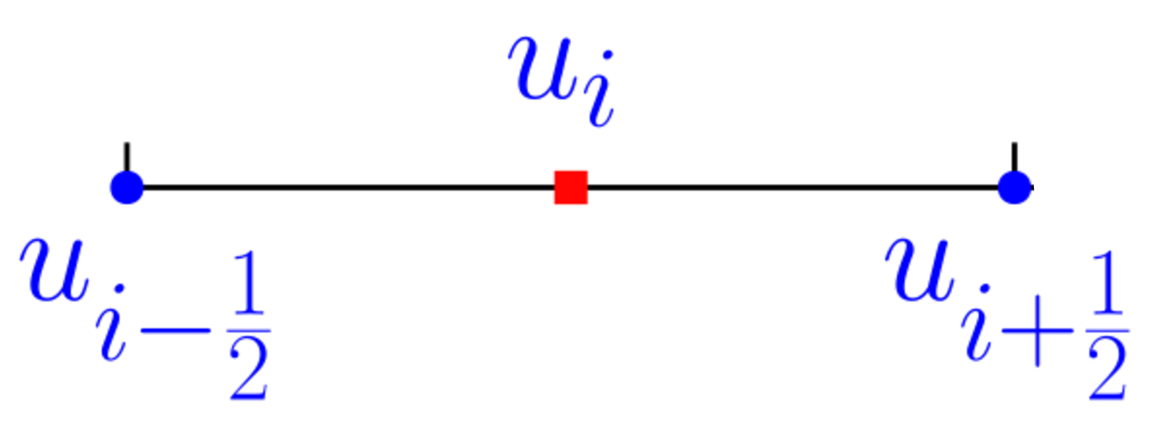
The three pieces of information accessible to each cell (two point values and the cell average) allow for a parabolic reconstruction \(u_{\text{recon},i} \colon \left[-\frac{\Delta x}{2}, \frac{\Delta x}{2} \right ]\), which fulfills \[\begin{align} u_{\text{recon},i}\left(\pm\frac{\Delta x}{2}\right) &= u_{i\pm\frac{1}{2}}, \qquad \frac{1}{\Delta x} \int_{-\frac{\Delta x}{2}}^{\frac{\Delta x}{2}} u_{\text{recon},i}(x) \,\mathrm{d}x = u_i. \end{align}\] One finds \(u_{\text{recon},i} = \frac{6 u_i - u_{i+\frac{1}{2}} - u_{i-\frac{1}{2}}}{4} + \frac{u_{i+\frac{1}{2}} - u_{i-\frac{1}{2}}}{\Delta x} x + 3\frac{u_{i+\frac{1}{2}} + u_{i-\frac{1}{2}} - 2 u_i}{\Delta x^2} x^2\). The global reconstruction \(u_\text{recon} (x) \colon \mathbb{R} \to \mathbb{R}\) is piecewise parabolic and continuous: \[\begin{align} u_\text{recon}(x) = u_{\text{recon},j}(x - x_j) \quad \text{if} \quad x \in [x_{j-\frac{1}{2}}, x_{j+\frac{1}{2}}], \quad j \in \mathbb{N}. \end{align}\]
When integrating the conservation law \[\begin{align} \partial_t u + \partial_x f(u) = 0 \label{eq:conslaw} \end{align}\tag{3}\] over the cell, Gauss’ law allows you to couple the cell averages and the point values: \[\begin{align} \frac{\mathrm{d}}{\mathrm{d}t} u_i + \frac{f(u_{i+\frac{1}{2}}) - f(u_{i-\frac{1}{2}})}{\Delta x} &= 0.\label{eq:avgupdategeneral} \end{align}\tag{4}\] Next, we need to determine the point value updates. In this paper, we restrict ourselves to one upwind and one central point update.
The semi-discrete upwind point update is given by \[\begin{align} \frac{\mathrm{d}}{\mathrm{d}t}u_{i+\frac{1}{2}} + f'(u_{i+\frac{1}{2}})(d^\text{upw}_x u)_{i+\frac{1}{2}} &= 0 \label{eq:pointvalueupdategeneral} \end{align}\tag{5}\] combined with an upwind finite difference formula \((d^\text{upw}_x u)_{i+\frac{1}{2}}\): \[\begin{align} (d^\text{upw}_x u)_{i+\frac{1}{2}} := \begin{cases} \frac{\mathrm{d}}{\mathrm{d}x} u_\text{recon}(x_{i+\frac{1}{2}} - 0), & f'(u_{i+\frac{1}{2}}) > 0, \\\frac{\mathrm{d}}{\mathrm{d}x} u_\text{recon}(x_{i+\frac{1}{2}} + 0), & \text{else}, \end{cases} = \begin{cases} \frac{\mathrm{d}}{\mathrm{d}x} u_{\text{recon},i}\left(\frac{\Delta x}{2} \right), & if \quad f'(u_{i+\frac{1}{2}}) > 0, \\\frac{\mathrm{d}}{\mathrm{d}x} u_{\text{recon},i+1}\left(-\frac{\Delta x}{2} \right), & \text{else}. \end{cases} \label{eq:findiffgeneralupwind} \end{align}\tag{6}\] By construction, the finite differences are thus exact for parabolae. The discontinuity in the derivative of \(u_\text{recon}\) at \(x_{i+\frac{1}{2}}\) allows one to include upwinding. In [6], the scheme 4 6 has been found to be \(L^2\)-stable with RK3 up to a CFL number of about 0.4 using Fourier analysis.
For a positive advection velocity, we have \[\label{eq:upwind-AF-Dm} \frac{\dif}{\dif t} u_{i+1/2} + \frac{2 u_{i-1/2} - 6 u_{i} + 4 u_{i+1/2}}{\Delta x} = 0.\tag{7}\] For a negative advection velocity, we have \[\label{eq:upwind-AF-Dp} \frac{\dif}{\dif t} u_{i+1/2} - \frac{-4 u_{i+1/2} + 6 u_{i+1} - 2 u_{i+3/2}}{\Delta x} = 0.\tag{8}\] More about point updates in the Active Flux method can be found in [6] and papers therein. The semi-discrete Active Flux method can be extended to multiple dimensions and to higher orders of accuracy, see [42].
The point value update employing a central discretization will be used in the theoretical analysis below. A central derivative is obtained by taking the average of the two options 7 and 8 \[\begin{align} (d^\text{central}_x u)_{i+\frac{1}{2}} := \frac{1}{2} \left( \frac{\mathrm{d}}{\mathrm{d}x} u_{\text{recon},i}\left(\frac{\Delta x}{2} \right) + \frac{\mathrm{d}}{\mathrm{d}x} u_{\text{recon},i+1}\left(-\frac{\Delta x}{2} \right) \right ),\label{eq:findiffgeneralcentral} \end{align}\tag{9}\] which leads to the following update formula \[\label{eq:central95AF95point95values} \frac{\dif}{\dif t} u_{i+1/2} + \frac{u_{i-1/2} - 3 u_i + 3 u_{i+1} - u_{i+3/2}}{\Delta x} = 0.\tag{10}\]
The Active Flux method described above is conservative, since summing up the cell-averages 4 leads to conservation. The fact that the point updates inserted into this formula may themselves be found using a non-conservative update, does not change that 4 is conservative. Indeed 4 will guarantee by the Lax-Wendroff theorem that if the solution converges, it converges to a weak solution.
2.2 The summation-by-parts approach for showing energy stability↩︎
In the following, one-dimensional periodic first-derivative SBP operators are introduced. Consider a semi-discretization of the linear advection equation 2 with \(a=1\) supplemented by periodic
boundary conditions \[\frac{\dif}{\dif t} \pmb{u} + D \pmb{u} = \pmb{0},\] where \(\pmb{u}\) is the vector of unknowns and \(D\) the corresponding
difference operator. A SBP operator on the interval \(\Omega = [x_\mathrm{min}, x_\mathrm{max}]\) is associated to a vector \(\pmb{x}\) of discrete grid nodes within \(\Omega\) corresponding to the unknowns. Due to the matrix-vector formulation of SBP schemes, we use the notation \(\pmb{1} = (1, \dots, 1)^T\), \(\pmb{0} = (0, \dots,
0)^T\) for the values of these constant functions on the given grid.
A SBP operator \(D\) mimics the continuous integration-by-parts property on \(\Omega\) \[\begin{align}
\label{eq:ibp} \int_{x_{\min}}^{x_{\max}} v u_x \mathrm{d}x + \int_{x_{\min}}^{x_{\max}} v_x u \mathrm{d}x = vu\vert_{x_{\min}}^{x_{\max}}
\end{align}\tag{11}\] on the discrete level. Here, we restrict ourselves to periodic boundary conditions, i.e. 11 \(= 0\). Then, the periodic SBP property is given as
\[\begin{align} &(\mathbf{v}, D\mathbf{u})_M + (D\mathbf{v}, \mathbf{u})_M = 0,\label{eq:sbp}
\end{align}\tag{12}\] where \(M\) is the symmetric and positive definite norm matrix of the given SBP operator \(D\) with the inner product \((u,v)_M=\mathbf{u}^T M \mathbf{v}\).
Considering 2 with \(a=1\) and the periodicity of the problem we find \[\begin{align} \frac{\mathrm{d}}{\mathrm{d}t}\Vert u \Vert_{L^2(\Omega)}^2 &= 2 \int_{x_\mathrm{min}}^{x_\mathrm{max}} u \partial_t u \mathrm{d}x = -2 \int_{x_\mathrm{min}}^{x_\mathrm{max}} u \partial_x u \mathrm{d}x = -u^2(x_\mathrm{max}, t)+u^2(x_\mathrm{min}, t) = 0\label{eq:intro95continous95energy} \end{align}\tag{13}\] from 11 . Using the SBP operator \(D\) with 12 , the corresponding semi-discrete operation yields \[\begin{align} \frac{\dif}{\dif t} \| \pmb{u} \|_M^2 &= 2 \pmb{u}^T M \frac{\dif}{\dif t} \pmb{u} = -2 \pmb{u}^T M D \pmb{u} = - \pmb{u}^T M D \pmb{u} + \pmb{u}^T D^T M \pmb{u} = 0,\label{eq:intro95discrete95energy} \end{align}\tag{14}\] and energy stability is ensured. A periodic SBP operator approximating \(\partial_x\) is classically defined as follows:
Definition 1. A periodic SBP operator* on the interval \([x_\mathrm{min}, x_\mathrm{max}]\) consists of a grid \(\pmb{x}\), a consistent derivative matrix \(D\) (with \(D\pmb{1}=\pmb{0}\) and \(D\pmb{x}=\pmb{1}\)), and a symmetric and positive definite mass matrix \(M\) (also denoted as norm matrix) such that the periodic SBP property \[\label{eq:SBPproperty} M D + D^T M = 0\tag{15}\] holds. Since \(\int_{x_\mathrm{min}}^{x_\mathrm{max}}\mathrm{d}x=x_\mathrm{max}- x_\mathrm{min}\), \(M\) is scaled such that \(\pmb{1}^T M \pmb{1} = x_\mathrm{max}- x_\mathrm{min}\). We call this SBP operator a diagonal-norm SBP operator if \(M\) is diagonal.*
As seen from Definition 1, the periodic SBP property means skew-symmetry of \(D\) with respect to \(M\).
A classical first-derivative SBP operator \(D\) results from central differences and fulfills 15 in the periodic case, where the norm matrix \(M\) assumes a role similar to quadrature rules in finite element discretizations. Upwind SBP operators are a special case of dual-pair operators. For periodic boundary conditions, dual-pair upwind SBP operators \(D_+,D_-\) discretizing the first derivative fulfill a similar property: \(MD_+ +(D_-)^T M = 0\). However, each of the operators \(D_+\) and \(D_-\) regarded separately is based on upwind differencing which leads to a built-in artificial dissipation when combined with flux splitting [43]–[45]. This approach stabilizes both linear and nonlinear problems while retaining the stability properties associated with SBP schemes. Here, we use the following definition:
Definition 2. A periodic upwind SBP operator* on the interval \([x_\mathrm{min}, x_\mathrm{max}]\) consists of a grid \(\pmb{x}\), a pair of consistent derivative matrices \(D_-\) and \(D_+\), and a symmetric and positive definite mass matrix \(M\) such that the periodic upwind SBP properties \[M D_+ + D_-^T M = 0, \qquad M (D_+ - D_-) \text{ is negative semidefinite}\] hold. Again, \(M\) is scaled to fulfill \(\pmb{1}^T M \pmb{1} = x_\mathrm{max}- x_\mathrm{min}\). If \(M\) is diagonal, we speak of a diagonal-norm upwind SBP operator.*
Using periodic upwind SBP operators, a semi-discretization of the linear advection equation 2 with \(a=1\) is \[\frac{\dif}{\dif t} \pmb{u} + D_- \pmb{u} = \pmb{0}.\] This method is stable since \[\label{eq:upwind-SBP-stability} \begin{align} \frac{\dif}{\dif t} \| \pmb{u} \|_M^2 &= 2 \pmb{u}^T M \frac{\dif}{\dif t} \pmb{u} = -2 \pmb{u}^T M D_- \pmb{u} = - \pmb{u}^T M D_- \pmb{u} + \pmb{u}^T D_+^T M \pmb{u} = \pmb{u}^T M (D_+ - D_-) \pmb{u} \le 0. \end{align}\tag{16}\] The energy stability of the scheme \(\frac{\dif}{\dif t} \pmb{u} - D_+ \pmb{u} = \pmb{0}\) for \(a = -1\) is shown similarly.
3 Matrix analysis of the Active Flux method↩︎
The following section is dedicated to the analysis of the semi-discrete Active Flux method in the framework of SBP operators. The difficult part consists in finding a suitable mass matrix \(M\) whereas the discrete derivative operator \(D\) corresponding to the Active Flux method can be constructed in a straightforward fashion. For this purpose, the Active Flux scheme 4 and the point update 5 for the linear scalar advection equation \(\partial_t u + \partial_x u = 0\) needs to be rewritten in matrix-vector form. Since periodic boundary conditions are considered, we identify \(u_{n-\frac{1}{2}} := u_{-\frac{1}{2}}\). In order to prove SBP properties, we will start with a central version of the Active Flux method since its SBP properties are easier to detect. Afterwards, in the subsequent section, we will turn to the standard upwind version of the Active Flux method.
3.1 Central Active Flux discretization↩︎
As motivated before, we aim at formulating the central version of the semi-discrete Active Flux method (given by 4 and 9 ) within the framework of SBP operators which immediately yields stability. The first step to reach this goal consists in establishing a matrix-vector formulation.
We begin by recalling that for the cell averages, the semi-discrete Active Flux method yields the update \[\frac{\dif}{\dif t} u_i + \frac{u_{i+1/2} - u_{i-1/2}}{\Delta x} = 0\,.\] We also recall that the point values are updated using a central discretization according to 9 , which yields \[\frac{\dif}{\dif t} u_{i+1/2} + \frac{u_{i-1/2} - 3 u_i + 3 u_{i+1} - u_{i+3/2}}{\Delta x} = 0.\] Collecting the cell averages \(u_{i}\) and the point values \(u_{i+1/2}\) in a single vector \(\pmb{u} \in \mathbb{R}^{2n}\), we can write the semi-discrete system in matrix-vector form as \[\label{eq:central-AF} \frac{\dif}{\dif t} \underbrace{\left(\begin{array}{c} \vdots \\ u_{i-1} \\\hline u_{i-1/2} \\ u_{i} \\\hline u_{i+1/2} \\ u_{i+1} \\\hline \vdots \end{array}\right)}_{=:\, \pmb{u}} + \underbrace{\frac{1}{\Delta x} \left(\begin{array}{cc|cc|cc|c} \ddots &&&\\ -1 & 0 & 1 &&\\\cline{1-6} 1 & -3 & 0 & 3 & -1 &&\\ && -1 & 0 & 1 &&\\\hline && 1 & -3 & 0 & 3 & -1 \\ &&&& -1 & 0 & 1 \\\cline{3-7} \multicolumn{4}{l|}{}&&& \ddots \end{array}\right)}_{=: \, D} \pmb{u} = \pmb{0}\tag{17}\] and directly obtain the discrete derivative operator \(D\). Here and below, we add guiding lines to the matrices to make it easier to see which entries belong to point values and cell averages.
We observe that \(D\) is skew-symmetric with respect to the diagonal mass matrix \[\label{eq:central-AF-diagonal-mass} M = \frac{\Delta x}{4} \left(\begin{array}{cc|cc|cc|c} \ddots &&\\ & 3 & \\\cline{1-4} & & 1 & & \\ && & 3 & \\\cline{3-6} \multicolumn{4}{l|}{} & 1 & & \\ \multicolumn{4}{l|}{} && 3 & \\\cline{5-7} \multicolumn{6}{l|}{}& \ddots \end{array}\right)\tag{18}\] since \[M D = -D^T M.\] Therefore, since \(M\) is diagonal with positive entries, the discretization of \(\partial_x\) via the Active Flux method yields a periodic SBP operator according to Definition 1. Hence, we have proved the following theorem.
Theorem 1. The central version 9 of the semi-discrete Active Flux method can be formulated using SBP operators with derivative matrix \(D\) 17 and diagonal norm/mass matrix \(M\) 18 , satisfying \(\pmb{1}^T M \pmb{1} = x_\mathrm{max}- x_\mathrm{min}\).
The diagonal mass matrix \(M\) in 18 can be interpreted as a chained trapezoidal rule in each cell. Using the transformation of the cell averages \(u_i = \frac{1}{6} u_{i - \frac{1}{2}} + \frac{2}{3} u_{i,p} + \frac{1}{6} u_{i + \frac{1}{2}}\) to the cell midpoints \(u_{i,p}\) derived from the reconstruction \(u_{\text{recon},i}\) and inserting this for the terms \(\frac{3}{4} u_i\) shows \[\begin{align} \pmb{1}^T M \pmb{u} &= \Delta x \left(\dots + \frac{1}{4} u_{i - \frac{1}{2}} + \left(\frac{1}{8} u_{i - \frac{1}{2}} + \frac{1}{2} u_{i,p} + \frac{1}{8} u_{i + \frac{1}{2}}\right) + \frac{1}{4}u_{i+1/2} + \left(\frac{1}{8} u_{i + \frac{1}{2}} + \frac{1}{2} u_{i+1,p} + \frac{1}{8} u_{i + \frac{3}{2}}\right) + \dots\right). \end{align}\]
Summing up the point values at cell interfaces and midpoints, we obtain the two variants \[\begin{align} \pmb{1}^T M \pmb{u} &= \frac{\Delta x}{2} \left(\dots + u_{i - \frac{1}{2}} + u_{i,p} + u_{i + \frac{1}{2}} + u_{i+1,p} + \dots\right)\\ &= \frac{\Delta x}{2} \left(\dots + \left(\frac{1}{2} u_{i - \frac{1}{2}} + u_{i,p} + \frac{1}{2} u_{i + \frac{1}{2}}\right)+ \left(\frac{1}{2} u_{i + \frac{1}{2}} + u_{i+1,p} + \frac{1}{2} u_{i + \frac{3}{2}}\right) \dots\right). \end{align}\] Thus, the quadrature induced by the diagonal mass matrix \(M\) defined by 18 can be considered either as the chained trapezoidal rule on the complete computational domain or in each individual cell. In fact, transferred to the interface and midpoint nodes \(u_i, u_{i,p}\) this quadrature rule directly corresponds to the diagonal mass matrix of the classical second-order SBP operator on equidistant nodes with grid spacing \(\frac{\Delta x}{2}\).
If we only focused on the central Active Flux method, we might stop here since diagonal norm/mass matrices offer the best structure for many types of equations. However, we are interested in the upwind version of the Active Flux method, as this version is more commonly used in practice. It will become clear in the following sections that we cannot use the diagonal mass matrix \(M\) 18 for the upwind case. Therefore, here, we continue to explore a more general class of mass matrices.
Among diagonal matrices, 18 is unique up to a scalar factor. Allowing for non-diagonal \(M\), a mass matrix which induces the SBP property is not unique, as we can see in the following discussion. The additional parameters introduced here will be required for the upwind Active Flux method. Firstly, the following lemma shows the non-uniqueness of a symmetric mass matrix satisfying \(M D = -D^T M\).
Lemma 1. All the symmetric, pentadiagonal matrices (up to boundary terms) which ensure that the derivative operator \(D\) of the central semi-discrete Active Flux method 17 is skew-symmetric with respect to \(M\), are of the form \[\label{eq:central-AF-banded-mass} M = \Delta x \left(\begin{array}{cc|cc|cc|cc|c} & & \text{\rotatebox{10}{\ddots}} & && \\ & m_{vv} & \frac{m_v-3 m_p}{2} & m_v & \frac{m_v-3 m_p}{2} & m_{vv} \\\cline{1-8} && \frac{3 m_p - m_v+2m_{vv}}{6}& \frac{m_v-3 m_p}{2} & m_p & \frac{m_v-3 m_p}{2} & \frac{3 m_p - m_v+2m_{vv}}{6} & \\ &&& m_{vv} & \frac{m_v-3 m_p}{2} & m_v & \frac{m_v-3 m_p}{2} & m_{vv} \\\cline{3-9} \multicolumn{4}{l|}{} &&& \text{\rotatebox{10}{\ddots}} & & \\ \end{array}\right)\qquad{(1)}\] with \(m_p, m_v, m_{vv} \in \mathbb{R}\).
Proof. Due to the alternate setting of point values and cell averages in the Active Flux method, we use the ansatz \[M = \Delta x \left(\begin{array}{cc|cc|cc|cc|c} & & \ddots & && \\ & m_{vv} & m_{vp} & m_v & m_{vp}' & m_{vv} \\\cline{1-8} && m_{pp} & m_{vp}' & m_p & m_{vp} & m_{pp} &\\ &&& m_{vv} & m_{vp} & m_v & m_{vp}' & m_{vv} \\\cline{3-9} \multicolumn{4}{l|}{}&& & \ddots & & \\ \end{array}\right),\] where \(m_v\) and \(m_p\) are on the diagonal of \(M\) corresponding to the cell average (volume) and the point values, respectively. The skew symmetry \(M D + D^T M = 0\) requires \[\begin{align} m_{vp}' - m_{vp} &= 0,\\ 3 m_{pp} + m_{vp} - m_{vv} &= 0, \tag{19} \\ 3 m_p - 3 m_{pp} + m_{vp}' - m_v + m_{vv} &= 0, \tag{20} \end{align}\] from which we directly obtain \(m_{vp}' = m_{vp}\). Using this and adding the last two equations 19 , 20 we can solve for \(m_{vp}\) and then for \(m_{pp}\). Thus, we obtain \[\begin{align} \label{eq:mpp95mvp} m_{pp} &= \frac{3 m_p - m_v+2m_{vv}}{6}, \quad m_{vp} = \frac{m_v - 3 m_p}{2}\,, \end{align}\tag{21}\] which leaves us with the structure of \(M\) as presented in ?? . ◻
The banded mass matrix ?? reduces to the diagonal mass matrix in 18 for \(m_{vv} = 0\), \(m_p = m_v / 3\), and \(m_v = \frac{3}{4}\).
Secondly, for the matrix \(M\) in ?? to qualify as a mass matrix of an SBP operator, we require \(M\) to be positive definite. In the following, we restrict the investigation to \(m_{vv} = 0\), since this will be required later for the upwind version of Active Flux. Moreover, setting \(m_{vv} \ne 0\) would result in a bigger stencil of \(M\) in comparison to the stencil of the derivative operators. The following lemma determines a range of parameters for which \(M\) is positive definite and gives one case of a positive semidefinite \(M\) with multiplicity one of the corresponding zero eigenvalue.
Lemma 2. For \(m_{vv} = 0\), the matrix \(M\) in ?? has the following properties.
If \(2 m_v / 9 < m_p < 2 m_v / 3\) and \(m_v > 0\), then \(M\) is positive definite.
If \(m_p = 2 m_v / 9\) and \(m_v > 0\) then \(M\) is positive semidefinite with an eigenvalue \(0\) of multiplicity \(1\).
The technical proof of Lemma 2 involving properties of circulant matrices can be found in Appendix 8.
For \(m_{vv} = 0\) and \(m_p \ne 2 m_v / 3\), it is possible to rescale the matrix \(M\) in ?? to satisfy the classical constraint \(\pmb{1}^T M \pmb{1} = x_\mathrm{max}- x_\mathrm{min}\). Thus, we obtain
Theorem 2. The central version 9 of the semi-discrete Active Flux method can be formulated using SBP operators with derivative matrix \[D = \frac{1}{\Delta x} \left(\begin{array}{cc|cc|cc|c} \ddots &&&\\ -1 & 0 & 1 &&\\\cline{1-6} 1 & -3 & 0 & 3 & -1 &&\\ && -1 & 0 & 1 &&\\\hline && 1 & -3 & 0 & 3 & -1 \\ &&&& -1 & 0 & 1 \\\cline{3-7} \multicolumn{4}{l|}{}&&& \ddots \end{array}\right), \label{eq:D-central-AF}\qquad{(2)}\] and positive definite mass matrix \[M = \frac{3 \Delta x}{8 m_v - 12 m_p} \left(\begin{array}{cc|cc|cc|cc|c} & & \text{\rotatebox{10}{\ddots}} & && \\ & & \frac{m_v-3 m_p}{2} & m_v & \frac{m_v-3 m_p}{2} & \\\cline{1-8} && \frac{3 m_p - m_v}{6}& \frac{m_v-3 m_p}{2} & m_p & \frac{m_v-3 m_p}{2} & \frac{3 m_p - m_v}{6} & \\ &&& & \frac{m_v-3 m_p}{2} & m_v & \frac{m_v-3 m_p}{2} & \\\cline{3-9} \multicolumn{4}{l|}{} && & \text{\rotatebox{10}{\ddots}} & & \\ \end{array}\right),\] for \(m_v>0\) and \(2 m_v / 9 < m_p < 2 m_v / 3\), satisfying \(\pmb{1}^T M \pmb{1} = x_\mathrm{max}- x_\mathrm{min}\).
Next, we will use the additional degrees of freedom introduced by the banded structure of the mass matrix \(M\) in Theorem 2 to generalize the results to the upwind version of the Active Flux method.
3.2 Upwind version of Active Flux↩︎
We first collect the formulas for the upwind semi-discrete Active Flux method. The cell average update is \[\label{eq:upwind-AF-average} \frac{\dif}{\dif t} u_i + \frac{u_{i+1/2} - u_{i-1/2}}{\Delta x} = 0,\tag{22}\] the upwind point value update for positive advection velocity (see 7 ) is \[\frac{\dif}{\dif t} u_{i+1/2} + \frac{2 u_{i-1/2} - 6 u_{i} + 4 u_{i+1/2}}{\Delta x} = 0,\] and for negative advection velocity (see 8 ), we have \[\frac{\dif}{\dif t} u_{i+1/2} - \frac{-4 u_{i+1/2} + 6 u_{i+1} - 2 u_{i+3/2}}{\Delta x} = 0.\]
The upwind versions of the Active Flux method correspond to the derivative operators \[\label{eq:upwind-AF} D_+ = \frac{1}{\Delta x} \left(\begin{array}{cc|cc|cc|c} \ddots &&&\\ -1 & 0 & 1 &&\\\cline{1-6} && -4 & 6 & -2 && \\ && -1 & 0 & 1 &&\\\cline{3-7} \multicolumn{4}{l|}{} & -4 & 6 & -2 \\ \multicolumn{4}{l|}{} & -1 & 0 & 1 \\\cline{5-7} \multicolumn{6}{l|}{} & \ddots \end{array}\right), \quad D_- = \frac{1}{\Delta x}\left(\begin{array}{cc|cc|cc|c} \ddots &&& \\ -1 & 0 & 1 &&\\\cline{1-6} 2 & -6 & 4 &&&&\\ && -1 & 0 & 1 &&\\\hline && 2 & -6 & 4 &&\\ &&&& -1 & 0 & 1 \\\cline{3-7} \multicolumn{6}{l|}{}& \ddots \end{array}\right).\tag{23}\] Unfortunately these operators are not upwind SBP operators with the diagonal mass matrix 18 . However we can still achieve this property using a banded mass matrix as for the central approximation above. In addition, restricting the band width of the mass matrix to the band width of the derivative operators results in uniqueness of the admissible mass matrix \(M\) up to a scalar factor.
Lemma 3. The symmetric matrix \[\label{eq:upwind-AF-banded-mass} M = \Delta x \left(\begin{array}{cc|cc|cc|cc|c} & & \text{\rotatebox{10}{\ddots}} & & & \\ & 0 & -m_v / 2 & m_v & -m_v / 2 & 0 \\\cline{1-8} && m_v / 6 & -m_v / 2 & 2 m_v / 3 & -m_v / 2 & m_v / 6 & \\ &&& 0 & -m_v / 2 & m_v & -m_v / 2 & 0 \\\cline{3-9} \multicolumn{4}{l|}{} && & \text{\rotatebox{10}{\ddots}} & & \\ \end{array}\right)\qquad{(3)}\] is — up to a scalar factor \(m_v \in \mathbb{R}\) — the only symmetric matrix which is pentadiagonal (up to boundary terms) and ensures that the derivative operators \(D_\pm\) of the upwind semi-discrete Active Flux method 23 are adjoint to each other with respect to \(M\).
Proof. We use the same ansatz as for the proof of Lemma 1. Then, the mutual adjointness \(M D_+ + D_-^T M = 0\) requires \(m_{vv}=0\) and \[\begin{align} m_{vp} - m_{vp}' &= 0 &6 m_{pp} + 4 m_{vp}' + m_v &= 0 \\ 6 m_p + 4 m_{vp} - m_v +2 m_{vp}'&= 0 &6 m_{pp} + 2 m_{vp} &= 0 \end{align}\] This yields \(m_{vp}=m_{vp}'=-m_v/2,\;m_p=2m_v/3,\;m_{pp}=m_v/6\) and hence ?? . ◻
Note that the matrix \(M\) in ?? is a special case of the matrix in ?? with \(m_p = 2 m_v / 3\). In this case, \(M\) is positive semidefinite as shown in the following lemma.
Lemma 4. The matrix \(M\) in ?? is positive semidefinite for \(m_v > 0\) with an eigenvalue \(0\) of multiplicity \(1\) and eigenvector \(\pmb{1}\).
Proof. A simple calculation shows that the rows of \(M\) sum up to zero. Thus, \(\pmb{1}\) is an eigenvector of \(M\) with eigenvalue \(0\). It is sufficient to consider the case \(m_v=1\) to study its multiplicity and to determine the sign of the other eigenvalues. Using Lemma 8, the matrix \(B_k\) associated with \(M\) for \(m_v=1\) is given by (with \(\theta = \frac{2\pi k}{n}\), \(k=0, \dots, n-1\)) \[\begin{align} B_k=\begin{pmatrix} 1 & -(1+e^{-i\theta})/2\\ -(1+e^{i\theta})/2 & (2+\cos{\theta})/3 \end{pmatrix} \end{align}\] and its characteristic polynomial is \[\begin{align} z^2 - \frac{z}{3} (5 + \cos \theta) + \frac{1}{6} (1 -\cos \theta). \end{align}\] Its value at \(z=0\) can only vanish if \(\theta = 0\). Thus, this eigenvalue only appears once. Furthermore, for \(\theta\in(0,2\pi)\), the eigenvalues are positive since the roots of the characteristic polynomial are given by \(z_{1,2}=\frac{1}{6}\left(\cos\theta+5\pm\sqrt{(\cos\theta+5)^2 -6(1-\cos\theta)}\right)>0\). ◻
Classical finite difference SBP operators have the scaling \(D \propto \Delta x^{-1}\) and \(M \propto \Delta x\). Remark [rem:trapezoidalinterpretation] demonstrates that this expected scaling of the mass matrix \(M\) also holds for the central Active Flux method. However, we cannot obtain the scaling \(M \propto \Delta x\) by imposing \(\pmb{1}^T M \pmb{1} = x_\mathrm{max}- x_\mathrm{min}\) since \(M \pmb{1} = \pmb{0}\) for the upwind Active Flux method. Thus, we need to consider another way to fix the free parameter \(m_v\) in ?? . To do so, we introduce the vector \(\pmb{1}_\text{avg} = (\dots, 0, 1, 0, 1, \dots)^T\) which has a value unity for all averages and zero for all point values. Then, we compute \[\begin{align} \frac{\pmb{1}_\text{avg}^T M \pmb{u}}{\Delta x \, m_v} = & \dots +\,\, u_{i-2} \,\,-\,\, u_{i-\frac{3}{2}} \,\,+\,\, u_{i-1} \,\,-\,\, u_{i-\frac{1}{2}} \,\,+\,\, u_i \,\,-\,\,u_{i+\frac{1}{2}} \,\,+\,\, u_{i+1} \,\, - \dots \end{align}\] In particular, we can choose \(\pmb{u} = \pmb{1}_\text{avg}\), resulting in \[\begin{align} \frac{\pmb{1}_\text{avg}^T M \pmb{1}_\text{avg}}{\Delta x \, m_v} = & \dots +\,\, u_{i-2} \,\,+\,\, u_{i-1} \,\,+\,\, u_i \,\,+\,\, u_{i+1} \,\, + \dots = \frac{x_\mathrm{max}- x_\mathrm{min}}{\Delta x}. \end{align}\] This shows that choosing \(m_v = 1\) yields \(\pmb{1}_\text{avg}^T M \pmb{1}_\text{avg} = x_\mathrm{max}- x_\mathrm{min}\), i.e., the expected scaling of the mass matrix \(M \propto \Delta x\) (when focusing only on the volume contributions).
Relaxing the definiteness condition to allow for a positive semidefinite mass matrix \(M\) still enables a stability proof for the Active Flux method via SBP properties as we will show in 4. At this point however, we still need to prove the upwind SBP property requiring that \(M (D_+ - D_-)\) is negative semidefinite. This is the subject of the following lemma.
Lemma 5. For \(M\) in ?? and the upwind operators \(D_\pm\) in 23 , the matrix \(M (D_+ - D_-)\) is symmetric and negative semidefinite for \(m_v > 0\).
Proof. Concerning the symmetry, we have \[\setcounter{MaxMatrixCols}{20} \frac{M (D_+ - D_-)}{m_v} = \left(\begin{array}{c|cc|cc|cc|cc|cc|cc|c} &&\text{\rotatebox{10}{\ddots}}& & & & & \\\cline{1-9} \dots & -8/3 & 5 & -6 & 5 & -8/3 & 1 & -1/3 &\\ \dots & 1 & -3 & 5 & -6 & 5 & -3 & 1 & 0 &\\\cline{1-11} & -1/3 & 1 & -8/3 & 5 & -6 & 5 & -8/3 & 1 & -1/3 &\\ &&0 & 1 & -3 & 5 & -6 & 5 & -3 & 1 & 0 &\\\cline{2-13} \multicolumn{3}{l|}{} & -1/3 & 1 & -8/3 & 5 & -6 & 5 & -8/3 & 1 & -1/3 &\\ \multicolumn{3}{l|}{}&& 0 & 1 & -3 & 5 & -6 & 5 & -3 & 1 & 0& \\\cline{4-13} \multicolumn{5}{l|}{}&&&&& \text{\rotatebox{7}{\ddots}}& & & & \\ \end{array}\right).\]
Finally, using Lemma 8, one finds the eigenvalues to be 0 (\(n\) times) and (calling \(\theta := \frac{2\pi k}{n}\), \(k=0,\dots,n-1\)) \[\begin{align} -\frac{2}{3} \left(18 + 17 \cos \theta + \cos\left(2\theta \right)\right) < 0, \qquad \forall \theta. \end{align}\] ◻
Following the nomenclature introduced in [31] for central SBP operators, we combine the previous results (3, 4, and 5) and say that the semi-discrete Active Flux upwind operators \(D_\pm\) are degenerate upwind SBP operators when combined with the semidefinite mass matrix \(M\) ?? .
4 Stability of the Active Flux method via SBP properties↩︎
Since the central version of the Active Flux method can be formulated using SBP operators, we directly obtain stability.
Corollary 1. The central version 9 of the semi-discrete Active Flux method is stable for the linear advection 2 with periodic boundary conditions.
Proof. This follows immediately from Theorem 2 and classical stability properties of SBP operators. ◻
Unfortunately, the matrix \(M\) for which the upwind Active Flux operators \(D_\pm\) are mutually adjoint is only positive semidefinite. Thus, the classical energy stability proof does not guarantee stability immediately. However, based on 4, we can still obtain a stability result for the Active Flux method using the framework of SBP operators.
The idea is as follows. We show below that the states associated to zero energy are uniform (in space) constants. Thus, if the energy is decaying, it is generally speaking possible that a uniform constant could grow although its energy is zero. However, the time evolution of uniform constants is easy to check separately, and we find that uniform constants do not grow in time but are stationary.
Theorem 3. The upwind Active Flux semi-discretization \[\frac{\dif}{\dif t} \pmb{u} + D_- \pmb{u} = \pmb{0}\] using 22 and 7 of the linear advection equation \[\partial_t u + \partial_x u = 0\] with periodic boundary conditions is stable.
Proof. Using 4, we decompose the vector \(\pmb{u} = \pmb{u}_0 + \pmb{u}_\perp\) into the components \(\pmb{u}_0 \propto \pmb{1}\) in the kernel of \(M\) and \(\pmb{u}_\perp \perp \pmb{1}\) in its orthogonal complement. Following the usual upwind SBP argumentation 16 , we obtain \[\begin{align} \frac{\dif}{\dif t} \| \pmb{u} \|_M^2 &= 2 \pmb{u}^T M \frac{\dif}{\dif t} \pmb{u} = -2 \pmb{u}^T M D_- \pmb{u} = - \pmb{u}^T M D_- \pmb{u} + \pmb{u}^T D_+^T M \pmb{u} \le 0, \end{align}\] where we have used 5. Since \(M \pmb{1} = \pmb{0}\), \(\| \pmb{u} \|_M = \| \pmb{u}_\perp \|_M\) and the component in the orthogonal complement is stable. The component in the kernel of \(M\) is constant in time and thus also stable, since \[\frac{\dif}{\dif t} \pmb{u}_0 = -D_- \pmb{u}_0 = \pmb{0}.\] Thus, the method is stable. ◻
5 Numerical experiment↩︎
To exemplify the theoretical stability results, we perform a numerical experiment based on the linear advection equation \(\partial_t u + \partial_x u = 0\) with periodic boundary conditions in the interval \([0, 2\pi]\) and the initial condition \(u(0, x) = \exp(\sin(x))\). We use the central and upwind semi-discrete Active Flux methods with 50 volumes and integrate the resulting ODE system in time using the five-stage, third-order explicit Runge-Kutta method RK3(2)5F[3S*+] of [46] with time step size \(\Delta t = \Delta x / 2\). We chose this method since it has been optimized for hyperbolic problems and includes an interval on the imaginary axis in its stability interval as required for stability of central operators.
The energy analysis presented in the previous sections concentrates on the effect of the spatial semi-discretization. When integrating the resulting ODE in time, the energy behavior also depends on the time integration scheme. While many explicit Runge-Kutta methods can be shown to cause additional dissipation for linear problems [47]–[50], the analysis of nonlinear problems is more complex [51]–[53]. Since we are interested in a quadratic energy, we could use a symplectic Runge-Kutta method such as the implicit midpoint rule to preserve the energy evolution caused by the semi-discretization in space, cf.sections IV.2.1 and IV.4.1 of [54]. However, we would like to avoid introducing fully implicit methods for hyperbolic problems. Thus, we apply the relaxation approach discussed and analyzed in [55]–[57] to modify an explicit Runge-Kutta method slightly so that the fully discrete energy evolution is purely caused by the spatial semi-discretization without additional influence of the time integration method.
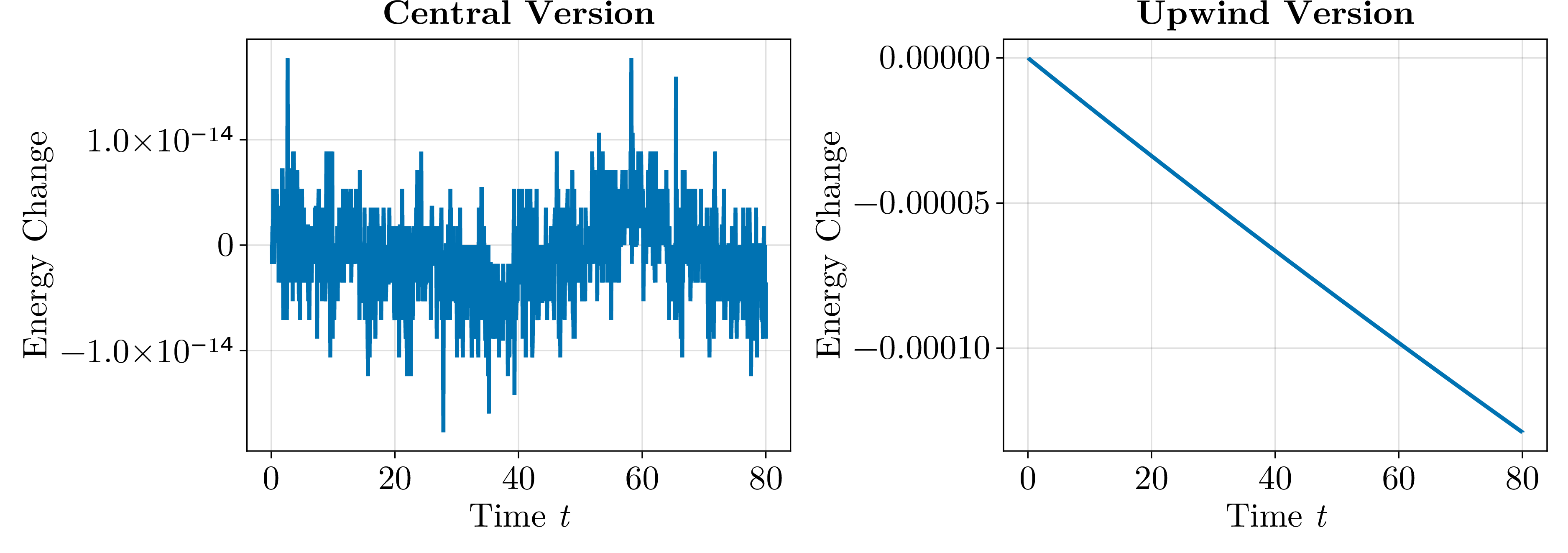
The results are shown in Figure 2. In accordance with the theory, the energy is conserved up to roundoff errors for the central version while the upwind version results in energy dissipation. All Julia [58] code and instructions required to reproduce these numerical experiments are available in our reproducibility repository [59]. We used CairoMakie.jl [60] to create the figures.
6 Nullspace consistency of the Active Flux upwind SBP operator↩︎
An additional property of the Active Flux difference operators which is not directly related to their upwind SBP property is nullspace consistency. This property is interesting on its own merit since it transfers an additional algebraic property from the continuous to the discrete setting. Nullspace consistency is a rather recently studied mimetic property in the context of derivative operators and numerical methods for PDEs. It signifies that the nullspace of the continuous operator is correctly transferred to its discrete counterpart. In the context of SBP schemes, this concept was first introduced in [61], connected to the investigation of convergence rates of FD schemes. According to the definition of nullspace consistency, for a nullspace-consistent finite difference operator \(D_k\) approximating the continuous operator \(\partial_x^k\), the kernel of \(D_k\) can be mapped one-to-one to the kernel of \(\partial_x^k\). In the context of periodic problems such as those studied in this work, nullspace consistency means that the creation of spurious modes within the discrete solution is prevented. The following lemma shows that upwind Active Flux difference operators are nullspace consistent.
Lemma 6. The Active Flux difference operators \(D_-\) and \(D_+\) are nullspace-consistent, i.e., \(D_\pm \pmb{u} = \pmb{0} \iff \pmb{u} \propto \pmb{1}\).
Proof. Due to symmetry, it is sufficient to consider \(D_-\) as the proof for \(D_+\) follows analogously. The nullspace of the linear continuous operator \(\partial_x\) consists of the functions constant in \(x\). Thus, we require that the only vectors \(\pmb{u}\) satisfying \(D_- \pmb{u} = \pmb{0}\) are the constants \(\pmb{u} = c \pmb{1}\).
Obviously, all vectors of the form \(\pmb{u} = c \pmb{1}\) satisfy \(D_- \pmb{u} = \pmb{0}\). It remains to show that all the vectors \(\pmb{u}\) with \(D_- \pmb{u} = \pmb{0}\) are of the form \(\pmb{u} = c \pmb{1}\). Then, all vectors in the nullspace of \(D_-\) have a counterpart in the nullspace of \(\partial_x\). The linear difference scheme resulting from the condition \(D_- \pmb{u} = \pmb{0}\) is \[\begin{align} \forall i&\colon& -u_{i-\frac{1}{2}}+u_{i+\frac{1}{2}} &=0,\\ \forall i&\colon& 2u_{i-\frac{1}{2}} - 6 u_i+4u_{i+\frac{1}{2}} &=0. \end{align}\] From the first equation, we obtain the existence of a constant \(c\in\mathbb{R}\) such that \(u_{i+\frac{1}{2}} = c\) is constant for all \(i\). Inserting this into the second equation then yields \(u_i = c\) for all \(i\), i.e., \(\pmb{u} = c \pmb{1}\). ◻
The central version of the Active Flux method is not nullspace consistent. This goes in line with the lack of nullspace consistency for periodic problems of the classical central second-order finite difference operator approximating the first derivative based on the approximation \(\partial_x u(x_i) \approx \frac{u_{i+1}-u_{i-1}}{2\Delta x}\).
Lemma 7. The central Active Flux difference operator \(D\) in 17 has a two-dimensional nullspace spanned by the vectors \(\pmb{1}\) and \((1,-1,1,-1,\ldots,1,-1)^T\). Therefore, the central version 9 of the Active Flux method is not nullspace-consistent.
Proof. As before, all vectors of the form \(\pmb{u} = c \pmb{1}\) obviously satisfy \(D \pmb{u} = \pmb{0}\). Furthermore, the linear difference scheme resulting from the condition \(D \pmb{u} = \pmb{0}\) is given by \[\begin{align} \forall i&\colon& -u_{i-\frac{1}{2}}+u_{i+\frac{1}{2}} &=0,\\ \forall i&\colon& u_{i-\frac{1}{2}} - 3 u_i + 3u_{i+1} - u_{i+\frac{3}{2}} &=0. \end{align}\] From the first equation, we again obtain that \(u_{i+\frac{1}{2}} = c\) is constant for all \(i\). Inserting this into the second equation now yields \(u_{i+1} = u_{i}=d\) for all \(i\), for a potentially different constant \(d\). Setting \(c=1\) and \(d=\pm1\) we obtain the two linearly independent vectors \(\pmb{1}\) and \((1,-1,1,-1,\ldots,1,-1)^T\) which span the nullspace of \(D\). ◻
On finite non-periodic domains, nullspace consistency for central difference approximations can be restored by suitable boundary closures [61].
7 Summary↩︎
To the best of our knowledge, we have proven stability using the summation-by-parts technique for an Active Flux method for the first time. To this end, we considered the linear advection equation on an interval with periodic boundary conditions. The Active Flux method, a finite volume method based on a globally continuous approach, has a cell average update plus point updates at the cell edges. We have studied two ways of updating the point values. First the point value updates using a central discretization 10 are chosen for purposes of theoretical analysis in 3.1. In 3.2 the commonly used upwind (see 7 and 8 ) version of the point value update is considered. Stability is shown for both cases in 4. In Section 5, we provide numerical examples illustrating stability, consistent with the theoretical results in this paper. In Section 6, we showed that the upwind Active Flux method is nullspace-consistent while the central one is not. As an additional bonus, the relation between energy stability via summation by parts and von Neumann stabiliy is shown in 9 for our PDE at hand.
Acknowledgments↩︎
The authors acknowledge funding by the Deutsche Forschungsgemeinschaft (DFG, German Research Foundation) within SPP 2410 Hyperbolic Balance Laws in Fluid Mechanics: Complexity, Scales, Randomness (CoScaRa), project numbers 525941602 (W.B., C.K., L.L.), 526073189 (S.O.) and 526031774 (H.R.). H.R. additionally acknowledges the DFG individual research grant 513301895. J.N. was supported by Vetenskapsrådet, Sweden [no. 2021-05484 VR] and University of Johannesburg Global Excellence and Stature Initiative Funding.
8 Properties of block circulant matrices and Proof of Lemma 2↩︎
Block circulant matrices [62], [63] are an extension of circulant matrices and possess the general form \[\label{eq:blockcirc} A = \begin{pmatrix} A_0 & A_1 & & & A_{n-1}\\ A_{n-1} & A_0 & A_1 & & \\ & A_{n-1} & A_0 & A_1 & &\\ & & & \ddots & &\\ A_1 & & &A_{n-1} & A_0 \end{pmatrix}\in \mathbb{R}^{nm\times nm},\tag{24}\] with \(A_k\in\mathbb{R}^{m\times m}\) for \(k=0,\ldots,n-1\).
The semi-discrete Active Flux method in one space dimension on a periodic domain yields block circulant matrices \(D_+,D_-\) and \(M\) and consequently also \(M(D_+-D_-)\) has a block circulant structure. Due to the alternating difference formulas for point values and for cell averages, the involved matrices hereby possess a specific structure of \(2\times2\) subblocks \[A_k=\begin{pmatrix} a_k & a_{k+1}\\ b_k & b_{k+1}\end{pmatrix},\quad k=0,\ldots,n-1.\] We may thus exploit the theory of block circulant matrices to obtain eigenvalues and eigenvectors of the given matrices.
Lemma 8 (Eigenvalues of block circulant matrices). The eigenvalues of the \(nm \times nm\) matrix 24 are the eigenvalues of all matrices \[\label{eq:Bk} B_k = A_0+r^k A_1+ \ldots r^{k(n-1)}A_{n-1}, \qquad k=0,1,\ldots,n-1,\qquad{(4)}\] with \(r=\mathrm{e}^{2\pi \mathrm{i}/n}\) the roots of unity. If \(\lambda\) is an eigenvalue of \(B_k\) with corresponding eigenvector \(v\), then \(\lambda\) is also an eigenvalue of \(A\) with eigenvector \((v^\mathrm{T}, r^k v^\mathrm{T}, r^{2k} v^\mathrm{T}, \ldots, r^{(n-1)j} v^\mathrm{T} )^\mathrm{T}\).
Proof. Consider the following ansatz for an eigenvector of \(A\) \[\begin{align} e_k = (v^\mathrm{T}, r^k v^\mathrm{T}, r^{2k} v^\mathrm{T}, \ldots, r^{(n-1)j} v^\mathrm{T} )^\mathrm{T}, \qquad k = 0, 1, \ldots, n-1, \end{align}\] for some yet to be determined \(v \in \mathbb{C}^m\). Then, \(A e_k = \lambda_k e_k\) if \[\begin{align} A e_k &= \begin{pmatrix} A_0 v + r^k A_1 v + \ldots + r^{(n-2)k}A_{n-2} v + r^{(n-1)k} A_{n-1} v \\ A_{n-1} v + r^k A_0 v + r^{2k} A_1 v + \ldots + r^{(n-1)k} A_{n-2} v\\ \vdots \\ A_1 v + \ldots + r^{(n-3)k} A_{n-2} v + r^{(n-2)k} A_{n-1} v + r^{(n-1)k} A_0 v \end{pmatrix} = \lambda_k \begin{pmatrix} v \\ r^k v \\ \vdots \\ r^{(n-1)k} v \end{pmatrix}. \end{align}\] The \(i\)-th component of this equation is (\(i = 0, \ldots, n-1\)) \[\begin{align} \sum_{j = n-i}^{n-1} r^{(j-n+i)k} A_j v + r^{ik} \sum_{j=0}^{n-1 - i} r^{jk} A_j v &= \lambda_k r^{ik} v, \label{eq:singlelinecirculant} \end{align}\tag{25}\] which reduces to just one equation for all \(i\) upon the choice \(r = \exp\left( \frac{2\pi \mathrm{i}}{n} \right )\). Then, the eigenvalue problem reduces to \[\begin{align} \sum_{j=0}^{n-1} r^{jk} A_j v = B_k v &= \lambda_k v. \end{align}\] ◻
As shown in [62], all eigenvalues and eigenvectors of \(A\) can be obtained in this manner. In addition, while all circulant matrices can be diagonalized, block circulant matrices allow for block diagonalization. A block circulant matrix does not necessarily possess a complete set of linearly independent eigenvectors; however, it does so if the matrices \(B_k\) can all be diagonalized. In this case, the block circulant matrix can be diagonalized as well.
Lemma 9. Let \(F\in\mathbb{C}^{n\times n}\) be the unitary matrix with entries \(F_{jk}=\frac{1}{\sqrt{n}}r^{(j-1)(k-1)},\;r=e^{2\pi \mathrm{i}/n}\), and \(I_m=\operatorname{diag}(1,\ldots,1)\in \mathbb{R}^{m\times m}\). For a block circulant matrix \(A\in\mathbb{R}^{mn\times mn}\) as in 24 , we have \[\label{eq:blockdiag} (F^\ast\otimes I_m) A (F\otimes I_m) = \operatorname{diag}(B_0,\ldots,B_{n-1}),\qquad{(5)}\] with \(B_k,\;k=0,\ldots,n-1\) given in ?? .
Proof. Using \[F\otimes I_m=\frac{1}{\sqrt{n}}\begin{pmatrix}I_m & I_m & I_m &\cdots & I_m\\ I_m & rI_m & r^2I_m & \cdots & r^{n-1}I_m\\ I_m & r^2I_m & r^4I_m & \cdots & r^{2(n-1)}I_m\\ \vdots & & \vdots\\ I_m & r^{n-1}I_m & r^{2(n-1)}I_m & \cdots & r^{(n-1)^2}I_m\end{pmatrix}\] and \(r^n=1\), we first obtain \[A (F\otimes I_m) = \frac{1}{\sqrt{n}}\begin{pmatrix} B_0 & B_1 & B_2 & \cdots & B_{n-1}\\ B_0 & B_1r & B_2r^2 & \cdots & B_{n-1}r^{n-1}\\ \vdots & &&&\vdots\\B_0 & B_1r^{n-1} & B_2r^{2(n-1)} & \ldots & B_{n-1}r^{(n-1)^2} \end{pmatrix}\] with \(B_k\) given in ?? . Using \(F^\ast_{jk}=\frac{1}{\sqrt{n}}\bar{r}^{(j-1)(k-1)}\) with \(\bar{r}=e^{-2\pi \mathrm{i}/n}\), i.e., \[F^\ast\otimes I_m=\frac{1}{\sqrt{n}}\begin{pmatrix}I_m & I_m & I_m &\cdots & I_m\\ I_m & \bar{r}I_m & \bar{r}^2I_m & \cdots & \bar{r}^{n-1}I_m\\ I_m & \bar{r}^2I_m & \bar{r}^4I_m & \cdots & \bar{r}^{2(n-1)}I_m\\ \vdots & & \vdots\\ I_m & \bar{r}^{n-1}I_m & \bar{r}^{2(n-1)}I_m & \cdots & \bar{r}^{(n-1)^2}I_m\end{pmatrix},\] we have \[(F^\ast\otimes I_m) A (F\otimes I_m)=\frac{1}{n}\begin{pmatrix} nB_0 & p(r)B_1 & p(r^2)B_2 & \cdots & p(r^{n-1})B_{n-1}\\ p(r^{n-1})B_0 & nB_1 & p(r)B_2 & \cdots& p(r^{n-2})B_{n-1}\\ \vdots & & & \ldots & \vdots\\ p(r)B_0 & p(r^2)B_1 & p(r^3)B_2 &\cdots & nB_{n-1} \end{pmatrix},\] with \(p(z)=1+z+z^2+\ldots+z^{n-1}\), where we exploit \(\bar{r}^k=r^{n-k}\). Finally, for \(z=r^k\) with \(k\not=0\) we have \(p(z)=0\), since the values \(r^k,\;k=1,\ldots,n-1\) are the roots of \(z^n=1\) which differ from \(z=1\) and we may factorize \(z^n-1=(z-1)(1+z+z^2+\ldots +z^{n-1})\). Thus, the block-diagonal form ?? is proven. ◻
Proof of Lemma 2. We use Lemma 8 and the notation described there. The eigenvalues of \(M\) can then be determined by the eigenvalues of the matrices \(B_k\) which in this case are given by \[\begin{align} B_k = \left(\begin{array}{cc}m_p + 2m_{pp}\cos\theta & m_{vp}\left(1+e^{-\mathrm{i}\theta}\right)\\m_{vp}\left(1+e^{\mathrm{i}\theta}\right)&m_v\end{array}\right), \quad \theta := \frac{2\pi k}{n}, \end{align}\] with \(m_{pp}\) and \(m_{vp}\) determined by 21 . The characteristic polynomial \(p\) of \(B_k\) is given by \[\begin{align} p(z)= z^2-tz+d \end{align}\] with \(t\) and \(d\) the trace and determinant of \(B_k\), respectively, \[\begin{align} t &= \mathrm{trace}(B_k) = \frac{1}{3} \left(3(m_p + m_v) + (3m_p-m_v) \cos\theta\right),\\ d &= \det{B_k} = \frac{1}{6} \left( -3(9 m_p^2 - 8 m_p m_v+m_v^2) - (9 m_p - 5 m_v)(3 m_p-m_v)\cos\theta \right). \end{align}\] We are now interested in a range of parameters \(m_v,m_p\) for which \(B_k\) has only positive eigenvalues for any value of \(\theta\). From the solution formula of quadratic equations it is clear that for positive solutions one requires \(t>0\) and \(d>0\) which yields the following inequalities regarding the coefficients of the characteristic polynomial: \[\begin{align} 3(m_p + m_v) + (3m_p-m_v) \cos\theta &>0, \tag{26}\\ -3(9 m_p^2 - 8 m_p m_v+m_v^2) - (9 m_p - 5 m_v)(3 m_p-m_v)\cos\theta &>0. \tag{27} \end{align}\] The latter inequality can be rewritten as \[\begin{align} m_v^2 -(9 m_p - 2 m_v)(3m_p - 2m_v) - \left( (9 m_p - 2 m_v)(3 m_p-2m_v) + m_v^2\right ) \cos\theta &>0 \label{eq:quadraticintermed} \end{align}\tag{28}\] i.e. \[\begin{align} m_v^2 -s- \left( s + m_v^2\right ) \cos\theta &>0 \end{align}\] with \(s:= (9 m_p - 2 m_v)(3 m_p-2m_v)\). For \(m_v > 0\), we obtain \(s<0\) precisely for \(2 m_v / 9 < m_p < 2 m_v / 3\). In that case, by the strict triangle inequality, we have \[\begin{align} |s + m_v^2| < |s| + m_v^2 = m_v^2 - s. \end{align}\] Since the condition \(a + b \cos \theta > 0\) for all \(\theta\) is equivalent to \(|b| < a\), one thus has proven 27 for the range of parameters considered in the first statement of the Lemma. Furthermore, simply with \(m_p, m_v > 0\) one obtains \[\begin{align} |3m_p - m_v| \leq 3|m_p| + |m_v| < 3 (m_p + m_v) \end{align}\] and thus 26 by the same argument. Thereby, we have proven the assertion that \(M\) possesses only positive eigenvalues if \(m_v>0\) and \(2 m_v / 9 < m_p < 2 m_v / 3\).
Finally considering the case of positive semidefinite matrices \(M\), we note that the characteristic polynomial \(p\) may have a zero eigenvalue, which is the case if and only if \(d=\det{B_k}=0\). For instance, this happens if
\(\theta = 0\) and either \(m_p = \frac{2 m_v}{9}\) or \(m_p = \frac{2 m_v}{3}\),
\(\theta = \pm \frac{\pi}{2}\) and \(m_p = \frac{4 \pm \sqrt{7}}{9} m_v = \begin{cases} 0.738... m_v > \frac{2}{3} m_v\,, \\ 0.150... m_v < \frac{2}{9} m_v\,. \end{cases}\)
Analogously, other values of \(\theta\) will likewise yield parameter values with \(B_k\) possessing a zero eigenvalue but will not be further studied here.
Considering the case \(m_p = \frac{2 m_v}{9}\), we have \(\det B_k = \frac{1}{6} m_v^2(1 - \cos \theta)\), which only vanishes for \(\theta=0\), and since we have \(\mathrm{trace}(B_k) \not=0\) for \(\theta=0,\;m_p = \frac{2 m_v}{9}\), the eigenvalue 0 has multiplicity 1. This proves the second statement of this lemma. The case \(m_p = \frac{2 m_v}{3}\) is treated in Lemma 3. ◻
9 Relation to von Neumann stability↩︎
Von Neumann stability uses the Fourier transform to make statements about the behavior in time of the \(L^2\) norm of the solution. In its restricted setting of linear problems on periodic domains it can also be used to derive a mass matrix that satisfies the periodic SBP property, as will be shown now.
9.1 General theory↩︎
Since averages and point values are independent, and since their nature and their update equations differ, when performing von Neumann stability analysis they need to be associated to independent Fourier modes. We thus write \[\begin{align} u_j &= \sum_{\omega} \hat{u}^\text{avg}(\omega) \exp(\mathrm{i}\omega j \Delta x) & u_{j-\frac{1}{2}} &= \sum_{\omega} \hat{u}^\text{point}(\omega) \exp(\mathrm{i}\omega j \Delta x) \end{align}\] The summation is over all wave numbers \(\omega\) that are compatible with the boundary conditions, i.e., \[\begin{align} q_{j+n} = \sum_{\omega} \hat{q}^\text{avg}(\omega) \exp(\mathrm{i}\omega (j+n) \Delta x) \equiv \sum_{\omega} \hat{q}^\text{avg}(\omega) \exp(\mathrm{i}\omega j \Delta x) = q_j \end{align}\] such that \[\begin{align} \omega \Delta x = 2 \pi \frac{k}{n} \qquad k = 0, \ldots, n-1. \end{align}\]
Since the method is linear, Fourier modes do not mix. From now on, we thus perform all calculations for just one of them and \(\omega\) is treated as a parameter. It is useful to introduce the translation operator \[\begin{align} \tau := \exp(\mathrm{i}\omega \Delta x) = \exp\left(2 \pi \frac{k}{n}\mathrm{i}\right). \end{align}\] Indeed, for a single Fourier mode, \[\begin{align} u_{j+1} &= \hat{u}^\text{avg}(\omega) \exp(\mathrm{i}\omega (j+1) \Delta x) = \tau u_j & \text{and similarly \quad } u_{j+\frac{1}{2}} &= \tau u_{j-\frac{1}{2}}. \end{align}\] The dependence of \(\tau\) on \(k\) shall not be made explicit in the notation.
In fact, \(\tau = r^k\) that has appeared previously in Lemma 8. The circulant matrices discussed in 8 have \(2\times 2\) blocks associated with one point value and one average. With \(A\) defined in 24 , inserting into \(A \pmb{u}\) a Fourier mode yields \[\begin{align} (A \pmb{u})_i = \sum_{j = n-i}^{n-1} A_{j} \hat{u} \tau^{j-n+i} + \sum_{j = 0}^{n-i-1} A_j \hat{u} \tau^{i+j} \overset{\tau^n = 1}{=} \tau^i \sum_{j = 0}^{n-1} A_j \hat{u} \tau^{j} = \tau^i B_k \hat{u} \end{align}\] where \(\hat{u} = \left( \begin{array}{c} \hat{u}^\text{point}\\\hat{u}^\text{avg} \end{array} \right)\). The parallel to Equation 25 is obvious. While the matrices \(B_k\) have been so far only used to determine the eigenvalues of \(A\), in fact it makes sense to call \(B_k\) the Fourier symbol \(\hat{A}\) of \(A\) that will be henceforth denoted by a hat.
Consider a generic numerical method \[\begin{align} \frac{\dif}{\dif t} \pmb{u} + A \pmb{u} = 0. \end{align}\] Von Neumann stability analysis amounts to studying the eigenvalues of \(\hat{A}\). Using the diagonalization \(\hat{R}^{-1} \hat{\Lambda} \hat{R}\) of \(\hat{A}\) in \[\begin{align} \frac{\dif}{\dif t} \hat{R} \hat{u} + \hat{\Lambda} \hat{R} \hat{u} = 0 \end{align}\] and calling \(\hat{U} := \hat{R} \hat{u}\), each component \(\hat{U}_\ell\) of \(\hat{U}\) fulfills the ODE \[\begin{align} \frac{\dif}{\dif t} \hat{U}_\ell + \lambda_\ell \hat{U}_\ell = 0 \end{align}\] solved by \(\hat{U}_{\ell,0} \exp(-\lambda t)\). We have preservation of the norm of \(\hat{U}_\ell\) if \(\lambda\) is purely imaginary. Its norm decays if \(\lambda\) has positive real part.
9.2 Preservation of energy↩︎
Consider now a situation in which all eigenvalues of \(\hat{A}\) are purely imaginary. Then1 \[\begin{align} \hat{U}^\dagger \hat{U} = \hat{U}_{0}^\dagger \hat{U}_{0}, \end{align}\] i.e., the \(L^2\) norm of \(\hat{U}\) is preserved. The \(L^2\) norm of \(\hat{u}\) is not preserved, but it needs to be weighted: \[\begin{align} \hat{U}^\dagger \hat{U} = \hat{u}^\dagger \hat{R}^\dagger \hat{R} \hat{u}. \end{align}\] Call \(\hat{M} := \hat{R}^\dagger \hat{R}\). One observes both the symmetry \(\hat{M}^\dagger = \hat{M}\) and the skew-symmetry of \(\hat{M} \hat{A}\): \[\begin{align} \hat{M} \hat{A} = \hat{R}^\dagger \hat{R} \hat{A} \underbrace{\hat{R}^{-1} \hat{R}}_{=\text{id}} = \hat{R}^\dagger \hat{\Lambda} \hat{R} = -(\hat{R}^\dagger \hat{\Lambda} \hat{R})^\dagger= -(\hat{R}^\dagger \hat{R} \hat{A})^\dagger = -(\hat{M} \hat{A})^\dagger, \end{align}\] where we have used \(\Lambda^\dagger = -\Lambda\). Thus, the Fourier symbol of the matrix \(M\) is simply \(\hat{R}^\dagger \hat{R}\), with as many free parameters as the dimension of the space on which \(\hat{M}\) acts, one for each free scaling parameter of the eigenvector.
Consider now \(A = D\), the space discretization of central Active Flux. \(\hat{D}\) reads \[\begin{align} \left( \begin{array}{cc} \frac{1}{\tau} - \tau & 3 - \frac{3}{\tau} \\ \tau - 1 & 0 \end{array} \right) \end{align}\] and its eigenvalues are \[\begin{align} \lambda^{\hat{D}}_\pm = \frac{\tau-1}{2\tau}\left(-\tau-1 \pm \sqrt{1 + 14 \tau + \tau^2}\right). \end{align}\] They are indeed imaginary, since upon the transformation \(\tau \mapsto \frac{1}{\tau}\) (complex conjugation) they map into their negative \[\begin{align} \frac{\frac{1}{\tau}-1}{2}\tau\left(-\frac{1}{\tau}-1 \pm \sqrt{1 + 14 \frac{1}{\tau} + \frac{1}{\tau^2}}\right) = -\frac{\tau-1}{2\tau}\left(-1-\tau \pm \sqrt{\tau^2 + 14 \tau + 1}\right) = - \lambda^{\hat{D}}_\pm. \end{align}\] An ingenious choice of normalization for the eigenvectors gives rise to the following Fourier symbol of the mass matrix: \[\begin{align} \hat{M} = \left( \begin{array}{cc} \alpha & \beta \\ \beta \tau & 3 \alpha + \beta (1+\tau) \end{array} \right ). \end{align}\] Here, \(\alpha\) and \(\beta\) are any Laurent polynomials in \(\tau\) under the condition that the matrix remains Hermitian. This is equivalent to \[\begin{align} \bar \beta &= \beta \tau, \label{eq:conditionbeta}\\ \bar \alpha &= \alpha. \end{align}\tag{29}\] If \(\beta = \sum_{\ell = -s}^s \beta_\ell \tau^\ell\), then condition 29 reads \[\begin{align} \bar \beta = \sum_{\ell = -s}^s \beta_\ell \tau^{-\ell} = \sum_{\ell = -s}^s \beta_{-\ell} \tau^{\ell} &= \sum_{\ell = -s+1}^{s+1} \beta_{\ell-1} \tau^{\ell} = \sum_{\ell = -s}^s \beta_\ell \tau^{\ell+1} = \beta \tau. \end{align}\] The first polynomials for \(s = 0, 1, 2, \dots\) that fulfill this are, up to scaling and linear combinations, \[\begin{align} 0, 1 + \frac{1}{\tau}, \tau + \frac{1}{\tau^2}, \ldots \end{align}\]
Similarly, \(\alpha\) must be symmetric upon the transformation \(\tau \mapsto \frac{1}{\tau}\), i.e. the first few polynomials (up to scaling and linear combinations) are \[\begin{align} 1, \tau + \frac{1}{\tau}, \tau^2 + \frac{1}{\tau^2}, \dots \end{align}\]
One choice is \(\beta = 0, \alpha = 1\), yielding matrix 18 , another is \[\begin{align} \alpha &= m_p + \frac{3 m_p - m_v + 2 m_{vv}}{6}\left( \tau + \frac{1}{\tau} \right) \in \mathrm{span}\left(1, \tau + \frac{1}{\tau}\right), \\ \beta &= -(3 m_p - m_v)\frac{1+\tau}{2 \tau} \in \mathrm{span}\left( 1 + \frac{1}{\tau} \right). \end{align}\] yielding ?? . Further choices can thus be systematically derived, for instance using \[\begin{align} \alpha &= m_p + y\left( \tau + \frac{1}{\tau} \right) + \frac{m_{vvv} - m_{vvp}}{3} \left( \tau^2 + \frac{1}{\tau^2} \right ) \in \mathrm{span}\left(1, \tau + \frac{1}{\tau}, \tau^2 + \frac{1}{\tau^2}\right), \\ \beta &= \frac{-3 m_p + m_v}{2}\left( 1 + \frac{1}{\tau}\right ) + m_{vvp} \left( \tau + \frac{1}{\tau^2} \right ) \in \mathrm{span}\left( 1 + \frac{1}{\tau}, \tau + \frac{1}{\tau^2} \right). \end{align}\] with \(y := \frac{3 m_p - m_v + 2 m_{vv} - 2 m_{vvp}}{6}\) one obtains \[\begin{align} {\text{\normalsize M =}} \left( \begin{array}{c|cc|cc|cc|cc|cc|cc|c} & &&& \text{\rotatebox{20}{\ddots}} &&&& \\\cline{1-11} &\frac{m_{vvv} - m_{vvp}}{3} & m_{vvp} & y & \frac{m_v-3m_p}{2} & m_p & \frac{m_v-3m_p}{2} & y & m_{vvp} & \frac{m_{vvv} - m_{vvp}}{3} & \\ & & m_{vvv} & m_{vvp} & m_{vv} & \frac{m_v-3m_p}{2} & m_v &\frac{m_v-3m_p}{2} & m_{vv} & m_{vvp} & m_{vvv} \\\cline{2-13} \multicolumn{3}{l|}{}&\frac{m_{vvv} - m_{vvp}}{3} & m_{vvp} & y & \frac{m_v-3m_p}{2} & m_p & \frac{m_v-3m_p}{2} & y & m_{vvp} & \frac{m_{vvv} - m_{vvp}}{3} & \\ \multicolumn{3}{l|}{}& & m_{vvv} & m_{vvp} & m_{vv} & \frac{m_v-3m_p}{2} & m_v &\frac{m_v-3m_p}{2} & m_{vv} & m_{vvp} & m_{vvv} \\ \cline{4-14} \multicolumn{5}{l|}{}&&&&& \text{\rotatebox{20}{\ddots}} &&&& \end{array} \right) \end{align}\]
References↩︎
The dagger denotes the Hermitian (conjugate) transpose.↩︎