On Conservative Matrix Fields: Continuous Asymptotics and Arithmetic
July 10, 2025
Abstract
Ratios of D-finite sequences and their limits – known as Apéry limits – have driven much of the work on irrationality proofs since Apéry’s 1979 breakthrough proof of the irrationality of \(\zeta(3)\). We extend ratios of D-finite sequences to a high-dimensional setting by introducing the Conservative Matrix Field (CMF). We demonstrate how classical Apéry limits are included by this object as special cases. A useful construction of CMFs is provided, drawing a connection to gauge transformations and to representations of shift operators in finite dimensional modules of Ore algebras. Finally, numerical experiments on these objects reveal surprising arithmetic and dynamical phenomena, which are formulated into conjectures. If established, these conjectures would extend Poincaré–Perron asymptotics to higher dimensions, potentially opening the door to optimization-based searches for new irrationality proofs.
1 Introduction↩︎
D-finite sequences, also known as P-recursive, or holonomic sequences, are fundamental to many areas of mathematics, such as combinatorics [1], [2], transcendence [3], [4], identity proofs [5], and the theory of D-modules [6]. In 1979, Roger Apéry found that a ratio of two such sequences converged to \(\zeta(3)\) in such a way as to prove its irrationality [7]. His proof sparked a flurry of activity [8]–[13] and motivated deeper analysis of such ratios of D-finite sequences, as well as experimental analysis of such sequences [14]–[18].
Here we present Conservative Matrix Fields (CMFs) – a multi-dimensional framework extending classical ratios of D-finite sequences. Using CMFs, we define a generalization of such sequences that inherit their desirable properties regarding convergence and irrationality measures, while also exhibiting new properties such as continuous arithmetic and asymptotic expansions.
Early limited cases of CMFs appeared in a pioneering work by Bill Gosper for identity proofs and other applications [19]. Families of CMFs were later found to generalize rational approximations of fundamental constants [16], and construct a structured proof of the irrationality of Apéry’s constant [20]. A recent work used CMFs for unifying hundreds of formulas for \(\pi\) [21]. CMFs also generalize concepts such as WZ-pairs [5], and multivariate hypergeometric terms [22], [23].
The framework presented in this paper provides a systematic perspective on previous methods in the field: To find non-trivial irrationality measures of a desired constant \(c\), researchers evaluated multivariate D-finite functions \(f(\boldsymbol{x}),g(\boldsymbol{x}):\mathbb{Q}^d\to\mathbb{Q}\) at a linear sequence of points \(x+nv, x\in\mathbb{Q}^d,v\in\mathbb{Z}^d,n\in\mathbb{N}\) in some space of high dimension \(d\), generating a specific ratio of D-finite sequences \(\frac{f(x+nv)}{g(x+nv)}\) that converges to that desired constant (often expressed as \(f(x+nv)-c\cdot g(x+nv)\to 0\)). This method is most commonly implemented on multivariate integrals [9], [10], [18], as first presented by Beukers as an alternative proof for the irrationality of \(\zeta(3)\) [8]. Such multivariate D-finite functions yielded promising results and non-trivial irrationality measures. However, many aspects of these sequences remain to be explored, such as the dependence of the ratios on \(v\) – the direction of the sequence of evaluation points. Specifically, to the knowledge of the authors, no such analysis has been done on the asymptotic and arithmetic properties of the ratio of D-finite sequences \(\frac{f(x+nv)}{g(x+nv)}\), such as the ratio’s convergence rate and irrationality measure.
In this work, we provide a novel way of generating CMFs from multivariate D-finite functions. This construction relies on calculating representations of the shift operators in the image of the Ore Algebra as an action on the D-finite function. Next, we derive from CMFs a high-dimensional generalization of the ratios of D-finite sequences considered by Apéry and by following works. We analyze this object, which we term a ‘Conservative Matrix Field Ratio’. Employing computational experiments of CMF ratios, we show that they possess useful and surprising properties, like a continuity in the irrationality measure of the CMF ratios, as function of the direction \(v\) in \(\mathbb{Z}^d\). These apparent properties are formulated into concrete conjectures.
Looking forward, the proof of these conjectures could provide a new and useful perspective on D-finite functions, and their asymptotic and arithmetic properties. In addition, these properties suggest the application of optimization algorithms in the search for irrationality proofs.
The remainder of this paper is structured as follows. In Section 2 we include an accessible review of preliminary results. Ore algebras, D-finite functions, Poincaré Perron asymptotics, irrationality measures, Apéry limits, and finally conservative matrix fields. In Section 3 we introduce the construction of conservative matrix fields from multivariate D-finite functions, and some of its properties. In Section 4 we introduce the CMF ratio, and CMF limit, and demonstrate their relation to ratios of D-finite sequences, and to Apéry limits. Finally, in Section 5 we demonstrate the results of experimental analysis of some CMF ratios, discuss some observations, formalize them into conjectures, and discuss some special cases, applications, and corollaries. Many examples are provided throughout the paper.
2 Preliminaries↩︎
While there are plenty other more comprehensive sources regarding Ore algebras and D-finite functions [24], [25], Poincaré Perron asymptotics [2], [26], [27], and Apéry limits [17], [18], [28], the following sub-sections detail definitions, theorems, and notations that will be used later in this paper. The final sub-section regarding conservative matrix fields contains similarly core definitions and results.
2.1 Ore Algebra↩︎
Recall the definition of Ore algebras, as defined in [24]:
Definition 1. Let \(A\) be an integral domain, with \(\sigma\) endomorphism, and \(\delta\) a \(\sigma\)-derivation. Meaning \(\delta:A\to A\) is linear, and satisfies: \[\delta(ab) =\delta(a)b+\sigma(a)\delta(b)\] for all \(a,b\in A\)
Define \(A[\partial]\) as the ring of polynomials in \(\partial\), with non-commutative multiplication, satisfying for \(a\in A\): \[\partial a = \sigma(a)\partial + \delta(a)\] Then, \(\mathbb{A}\mathrel{\vcenter{:}}= (A[\partial],\sigma,\delta)\) is an Ore algebra* over \(A\).*
Example 1. While the generality of Definition 1 is useful, this work deals with two main Ore algebras. Let \(K\) be a field of characteristic \(0\). We consider two main Ore algebras:
\((K(z)[\theta_z],\text{Id},z\frac{d}{dz})\) - the algebra of Euler differential operators
\((K(x)[S],\sigma,0)\), where \(\sigma(x) = x+1\) - the algebra of recurrence operators. Satisfying \(Sf(x) = f(x+1)S\)
Ore algebras can be considered in the multivariate case, under further conditions.
Definition 2. For \(1\leq i\leq d\), let \(\mathbb{A}_i \mathrel{\vcenter{:}}= (A[\partial_i],\sigma_i,\delta_i)\) be Ore algebras, where the \(\sigma_i\)’s and \(\delta_i\)’s commute. One can define the non-commutative ring \(A[\partial_1,\dots, \partial_d]\) with each \(\partial_i\) satisfying the same commutation with field elements as in \(\mathbb{A}_i\), and also satisfying \(\partial_i\partial_j =
\partial_j\partial_i\).
Then, \(\mathbb{A}\mathrel{\vcenter{:}}=(A[\partial_1,\dots, \partial_d],\sigma_1,\dots,\sigma_d,\delta_1,\dots,\delta_d)\) is a (multivariate) Ore algebra* over \(A\).*
Example 2. an example of such extension is that of Ore Laurent polynomials. For example, for \(K\) field of characteristic 0, consider: \[\mathbb{A}' \mathrel{\vcenter{:}}=(K(x)[S,S^{-1}],\sigma,\sigma^{-1},0,0)\] Note that as \(\sigma\) commutes with its inverse, and as both derivations are the zero function, the conditions in Definition 2 hold.
Let us detail the multivariate Ore algebras that will be core to the theory of conservative matrix fields.
Remark 1. We will be interested in the following multivariate Ore algebras: \[\text{for } \boldsymbol{x} =(x_1,\dots,x_d),\boldsymbol{z} =(z_1,\dots,z_l),\quad \mathbb{A}=
K(\boldsymbol{x},\boldsymbol{z})[S_{x_1},\dots,S_{x_d},\theta_{z_1},\dots,\theta_{z_l}]\] \[\mathbb{A}' =
K(\boldsymbol{x},\boldsymbol{z})[S_{x_1},S_{x_1}^{-1},\dots,S_{x_d},S_{x_d}^{-1},\theta_{z_1},\dots,\theta_{z_l}]\] with \(S_{x_i}\) the shift operator of \(x_i\), and \(\theta_{z_i}\) the Euler differential of \(z_i\).
We will notate a shift in direction \(v\) for \(v = (v_1,\dots,v_d)\) (with \(v\in\mathbb{N}^d\) in \(\mathbb{A}\) and \(v\in\mathbb{Z}^d\) in \(\mathbb{A}'\)) as \(S_v\mathrel{\vcenter{:}}=\prod_{i=1}^dS^{v_i}_{x_i}\) and \(\sigma_v\) as the
appropriate composition of \(\sigma_i\)’s. Meaning, for \(f\in K(\boldsymbol{x},\boldsymbol{z})\): \[S_vf(x,z) = \sigma_v(f(x,z))S_v = f(x+v,z)S_v\] Note
\(S_vS_w = S_{v+w}\).
2.2 D-finite Functions↩︎
The ring of functions \(f\in F\mathrel{\vcenter{:}}= K(\boldsymbol{x})[[\boldsymbol{z}]]\) form a left module of the Ore algebras in Remark 1. We shall notate the action using a bottom dot: meaning for \(L\in\mathbb{A}\), its action on \(f\in F\) is notated as \(L.f\). Some such functions vanish under operators in an Ore algebra (\(L.f \equiv 0\)). This set of operators is called the annihilator ideal:
Definition 3. the Annihilator* of a function \(f(\boldsymbol{x},\boldsymbol{z})\in F\) in the Ore algebra \(\mathbb{A}= K(\boldsymbol{x},\boldsymbol{z})[S_{x_1},\dots,S_{x_d},\theta_{z_1},\dots,\theta_{z_l}]\) is the following set: \[\text{ann}(f) = \left\{ L\in \mathbb{A}: L.f = 0 \right\}\]*
Remark 2. \(\text{ann}(f)\subset \mathbb{A}\) is a left ideal of the Ore algebra \(\mathbb{A}\).
Often, the image of a function under a set of operators is also considered:
Definition 4. the image of a function \(f\in F\) under an Ore algebra \(\mathbb{A}\) is the following set: \[\mathbb{A}.f \mathrel{\vcenter{:}}= \left\{ L.f:L\in\mathbb{A} \right\}\]
Definition 5. A D-finite function* \(f\) is a function for which: \[\dim \mathbb{A}/\text{ann}(f) = \dim \mathbb{A}.f < \infty\] As vector spaces over \(K(\boldsymbol{x},\boldsymbol{z})\).*
Remark 3. \({}\)
The condition in Definition 5 is equivalent (and sometimes replaced by) either \(\dim \text{span}\left\{ \partial_i^k.f:k\in\mathbb{N} \right\}<\infty\) for all \(i\), or \(K[\partial_i]\cap \text{ann}(f)\neq\emptyset\) for all \(i\).
Note that for any \(f\in F\), \(S_{x_i}.f\equiv 0\iff f\equiv 0\). Thus implying, for \(f\in F\) D-finite, the minimal degree operator in \(K[S_{x_i}]\cap \text{ann}(f)\), \(\sum_{j=0}^r p_j S_{x_i}^j\) satisfies \(p_j\in K(\boldsymbol{x},\boldsymbol{z})\quad p_0,p_r\not\equiv0\)
Given that minimal operator \(\sum_{j=0}^r p_j S_{x_i}^j\), Note that: \[\left(\sum_{j=0}^r p_jS_{x_i}^j\right).f = 0\implies \left(-\sum_{j=1}^r \frac{p_j}{p_0}S_{x_i}^{j}\right).f = f\] \[\implies \left( -\sum_{j=1}^r \sigma_i^{-1}\left(\frac{p_j}{p_0}\right)S_{x_i}^{j-1}\right).f = \sigma_i^{-1}(f) = S_{x_i}^{-1}.f\]
The point above means that for \(f\in F\) D-finite over \(\mathbb{A}\), \(\mathbb{A}.f = \mathbb{A}'.f\)
Example 3. Examples of D-finite functions include:
The binomial \(f(n,k) = \binom{n}{k}\) is D-finite in \(\mathbb{A}= \mathbb{Q}(n,k)[S_{n},S_{k}]\)
Bessel Functions (such as \(J_n(z),I_n(z)\dots\)) are D-finite in \(\mathbb{A}= \mathbb{Q}(n,z)[S_n,\theta_z]\)
Generalized hypergeometric functions \(\begingroup \pFqmuskip=8mu\relax \mathcode`\,=\string"8000 \begingroup\lccode`\~=`\, \lowercase{\endgroup\let~}\mskip\pFqmuskip {}_{p}F_{q}{\left[\genfrac..{0pt}{}{x_1,\dots,x_p}{y_{1},\dots,y_{q}};z\right]} \endgroup\) are D-finite in \(\mathbb{A}= \mathbb{Q}(\boldsymbol{x},\boldsymbol{y},z)[S_{x_1},\dots,S_{y_q},\theta_z]\)
For the special case of a univariate Ore algebra \(K(n)[S_n]\) (recurrence operator algebra), D-finite functions are called D-finite Sequences or sometimes Holonomic or P-recursive sequences.
2.3 Poincaré Perron Asymptotics↩︎
The two landmark papers by Poincaré and Perron [26], [27], establish the asymptotic analysis of D-finite sequences. First, let us define the asymptotic of a function:
Definition 6. A function \(g(n)\) is an asymptotic* of \(f(n)\) if \(\lim_{n\to\infty}\frac{f(n)}{g(n)}=1\), and that is denoted as \(f(n)\sim g(n)\)*
Theorem 1. (Poincaré 1885, Perron 1921)3. Let \(L\in \mathbb{Q}(n)[S_n]\) satisfy: \[L =
\sum_{i=0}^r a_i(n)S_n^i\quad \text{s.t}\quad a_r = 1\;, \;\lim_{n\to\infty}a_i(n) = a_i\] Suppose further the roots (\(\lambda_1,\dots,\lambda_r\)) of the characteristic polynomial* \(\sum_{i=0}^r a_it^i\) satisfy: \[\left| \lambda_1 \right|>\left| \lambda_2 \right|>\cdots >\left| \lambda_r \right|\] Then, for any solution \(u(n)\)
of \(L\) (meaning \(L.u(n) = 0\)), either \(\exists_N :\forall_{n>N}\;u(n) =0\), or \(\lim_{n\to\infty}\frac{u(n+1)}{u(n)} =
\lambda_i\) for some \(i\).
If also \(\forall_n\;a_1(n)\neq 0\), then for each \(\lambda_i\) there exists a solution \(u(n)\) of \(L\) such that \(\lim_{n\to\infty}\frac{u(n+1)}{u(n)} = \lambda_i\).*
Remark 4. The roots (\(\lambda_1,\dots,\lambda_r\)) of the characteristic polynomial of \(L\in \mathbb{Q}(n)[S_n]\) will be referred to as the eigenvalues* of
the recurrence.
This, as when \(L\) is encoded as a companion matrix, the characteristic polynomial of the matrix is exactly the characteristic polynomial of the recurrence. Thus, the eigenvalues of the limit of the companion matrix as
\(n\to \infty\), are exactly the roots (\(\lambda_1,\dots,\lambda_r\))*
A well known corollary of the theorem of Poincaré and Perron is the following:
Corollary 1. If the conditions in Theorem 1 are satisfied, then each solution \(u(n)\) satisfies:
\[u(n)= \sum_{i=1}^r c_i\lambda_i^nf_i(n)\] where each \(\lambda_i^nf_i(n)\) is a solution to \(L\), the functions \(f_i(n)\) are independent of initial conditions, and satisfy \(\frac{f_i(n+1)}{f_i(n)}\to 1\).
The values of \(c_i\) depend linearly on the initial conditions, and will be referred to as multiplicative constants.
Corollary 2. If the conditions in Theorem 1 are achieved, then each non-zero solution \(u(n)\) satisfies: \[u(n)\sim c_j\lambda_j^nf_j(n)\] Where \(j\) is the index of the first non zero multiplicative constant. (\(j = \min\left\{ 1\leq i\leq r:c_i\neq 0 \right\}\))
Remark 5. Finding closed forms for \(c_i\) as functions of the initial conditions is not solved in the general case and is of general interest. [29], [30]
Corollaries 1,2 are highly useful for the theory of Apéry limits, which is discussed in the following sub-section.
2.4 Apéry Limits and the Irrationality Measure↩︎
Definition 7. Let \(L\in \mathbb{Q}(n)[S_n]\) be a recurrence operator of order at least \(2\). Furthermore, let \(u_1(n),u_2(n)\in\mathbb{Q}^{\mathbb{N}}\) be two solutions of \(L\). Then, if their ratio \(\frac{u_1(n)}{u_2(n)}\) converges, the limit of the ratio is called an Apéry limit. and the sequence itself will be referred to in this paper as a D-finite Ratio.
These D-finite ratios are at the core of many irrationality results [8]–[10], [12], [13] , and Apéry limits include \(\pi,\gamma,e,\) Catalan’s constant \(G\), and many more. In his seminal 1979 work, Roger Apéry proved the irrationality of \(\zeta(3)\)[7], by constructing a D-finite ratio that converges to it, and that satisfies Dirichlet’s criterion:
Theorem 2. (Dirichlet 1834) for \(l\in\mathbb{R}, p_n,q_n\in\mathbb{Z}\setminus\left\{ 0 \right\}\), if \(\left| \left\{ \frac{p_n}{q_n}:n\in\mathbb{N} \right\} \right| = \infty\), and \[\exists_{C,\delta>0}:\left| \frac{p_n}{q_n}-l \right|<\frac{C}{\left| q_n \right|^{1+\delta}}\] then \(L\notin\mathbb{Q}\).
Remark 6. Notice, for \(l\neq 0\) that this is equally true when comparing with the numerators: \[\exists_{C,\delta>0}:\left| \frac{p_n}{q_n}-l \right|<\frac{C}{\left| p_n \right|^{1+\delta}}\]
Proving irrationality in this manner requires sequences that balance rapid convergence with slow growth in their numerators and denominators. These notions require definitions:
Definition 8. For a sequence \(s_n\in\mathbb{Q}\), such that \(s_n\to l\), its irrationality measure sequence* is the sequence of real numbers \(\delta_n\) satisfying: \[\left| s_n-l \right| = \frac{1}{H(s_n)^{1+\delta_n}},\] where \(H(s_n)\) is the classical/naive height, meaning the maximum of the absolute value of the reduced numerator and denominator: \[H(c) \mathrel{\vcenter{:}}= \max\left\{ \left| a \right|,\left| b \right| \right\} \text{ s.t } a,b\in\mathbb{Z}, (a,b) = 1, \frac{a}{b} = c.\] The limit of \(\delta_n\), if it exists, will be called the irrationality measure of the sequence (\(\delta = \lim_{n\to\infty}\delta_n\)). A sequence is said to have trivial irrationality measure if \(\delta = -1\)*
Remark 7. This is related to the Dirichlet criterion, as \(\lim\sup \delta_n>0\implies l\notin\mathbb{Q}\) (assuming also \(s_n\) does not repeat any element infinitely many times).
Definition 9. For a sequence \(s_n\in\mathbb{Q}\), such that \(s_n\to l\), its convergence rate sequence* is defined as: \[\rho_n = \frac{\log\left| s_n-l \right|}{n}\] The limit of \(\rho_n\), if it exists, will be called the convergence rate of the sequence (\(\rho = \lim_{n\to\infty}\rho_n\)). A sequence is said to have trivial convergence rate if \(\rho = 0\).*
Definition 10. For a sequence \(s_n\in\mathbb{Q}\), such that \(s_n\to l\), its height sequence* is defined as: \[\eta_n = \frac{\log\left| H(s_n) \right|}{n}\] The limit of \(\eta_n\), if it exists, will be called the height of the sequence (\(\eta = \lim_{n\to\infty}\eta_n\)). A sequence is said to have trivial height if \(\eta = 0\)*
Remark 8. These 3 quantities are linked, as: \[\delta_n = -1-\frac{\rho_n}{\eta_n}\] Thus:
If any two of the sequences \(\left\{ \delta_n, \rho_n,\eta_n \right\}\) have finite non trivial limits, then the third one converges as well
If for \(s_n\) all three converge, then the sub-sequence \(s'_n \mathrel{\vcenter{:}}= s_{kn}\) (for \(k\in\mathbb{N}\setminus\left\{ 0 \right\}\)), has the same limit \(l\) and irrationality measure \(\delta\), and \(\rho' = k\rho, \eta' = k\eta\)
if the sequence \(s_n\) has non trivial convergence rate, and \(\liminf\eta_n<-\rho\), then by Remark 7 \(l\notin\mathbb{Q}\)
The final point in Remark 8 is the key for Apéry’s proof of the irrationality of \(\zeta(3)\)
Theorem 3. Consider the following D-finite equation: \[(n+2)^3u(n+2)-(2n+3)(17n^2+51n+39)u(n+1) +(n+1)^3 u(n) = 0\] and two solutions, \(u_1(n), u_2(n)\) satisfying the following initial conditions: \[u_1(0) = 0, u_1(1) = 6, u_2(0) = 1, u_2(1) = 5\] Then, the sequence \(s_n = \frac{u_1(n)}{u_2(n)}\) converges to \(\zeta(3)\), with convergence rate \(\rho = -8\log(\sqrt{2}+1)\) and height satisfying \(\limsup\eta_n\leq 4\log(\sqrt{2}+1)+3\) and thus satisfying \(\liminf\delta_n\geq\frac{4\log(\sqrt{2}+1)-3}{4\log(\sqrt{2}+1)+3}\approx0.08\dots\) proving \(\zeta(3)\notin\mathbb{Q}\)
Proof. Full proofs can be found in [7], [8], [20]. Here we demonstrate that \(\rho = -8\log(\sqrt{2}+1)\) , and outline the method for showing \(\limsup\eta_n\leq 4\log(\sqrt{2}+1)+3\).
Analyzing the D-finite equation, one can see the characteristic polynomial of the recurrence is \(t^2-34t+1\), and \(\lambda_1 = (\sqrt{2}+1)^4,\lambda_2 = (\sqrt{2}-1)^4\). Thus Theorem 1 applies, and we can write: \[u_1(n) = c_1\lambda_1^nf_1(n)+c_2\lambda_2^nf_2(n),u_2(n) =
\tilde{c_1}\lambda_1^nf_1(n)+\tilde{c_2}\lambda_2^nf_2(n)\] Also notice that as the initial conditions are linearly independent, and hence so are \((c_1,c_2),(\tilde{c_1},\tilde{c_2})\). Thus: \[\frac{u_1(n)}{u_2(n)} = \frac{c_1\lambda_1^nf_1(n)+c_2\lambda_2^nf_2(n)}{\tilde{c_1}\lambda_1^nf_1(n)+\tilde{c_2}\lambda_2^nf_2(n)}\] As we assume \(\frac{u_1(n)}{u_2(n)}\to\zeta(3)\), we get
\(\frac{c_1}{\tilde{c_1}} = \zeta(3)\). And the convergence rate sequence satisfies: \[\rho_n = \frac{1}{n}\log\left| \frac{u_1(n)}{u_2(n)}-\frac{c_1}{\tilde{c_1}} \right| = \frac{\log\left|
\tilde{c_1}c_2-c_1\tilde{c_2} \right|+\log\left| f_2(n) \right|-\log\left| \tilde{c_1} \right|}{n}+\log\left| \lambda_2 \right|-\frac{1}{n}\log\left| u_2(n) \right|\] \[\implies \rho = \lim_{n\to\infty}\rho_n = \log\left|
\lambda_2 \right|-\log\left| \lambda_1 \right| = -8\log(\sqrt{2}+1)\] Also, It is possible to show that \(u_2(n),u_1(n)\cdot\text{lcm}(1,\dots,n)^3\in\mathbb{Z}\). Thus: \[\frac{u_1(n)}{u_2(n)} = \frac{u_1(n)\text{lcm}(1,\dots,n)^3}{u_2(n)\text{lcm}(1,\dots,n)^3}\implies \eta_n\leq\frac{\log\left| u_2(n)\text{lcm}(1,\dots,n)^3 \right|}{n}\to 4\log(\sqrt{2}+1)+3\] giving the result \(\limsup\eta_n\leq 4\log(\sqrt{2}+1)+3\). ◻
This flow regarding the convergence rate can be generalized. The following proposition essentially shows that for some D-finite ratios, their Apéry limits are ratios of coefficients of the asymptotic expansion, and their convergence rate is of the form \(\log\left| \frac{\lambda_k}{\lambda_j} \right|\), for some \(k>j\).
Proposition 4. Let \(L\) be a D-finite recurrence \(L\in \mathbb{Q}(n)[S_n]\) which satisfies the Poincaré-Perron conditions in Theorem 1. Furthermore, let \(u_1(n),u_2(n)\) be two linearly independent solutions of \(L\).
Then they result in a non-zero Apéry limit (\(\lim_{n\to\infty}\frac{u_1(n)}{u_2(n)}\in\mathbb{R}\setminus\left\{ 0 \right\}\)) if and only if the index of the first non-zero multiplicative constant is equal for both \(u_1(n),u_2(n)\). Namely: \[\min\left\{ 1\leq i\leq r:c_i\neq 0 \right\}=\min\left\{ 1\leq i\leq r:\tilde{c_i}\neq 0 \right\}\] Where \(u_1(n) =
\sum_{i=1}^rc_i\lambda_i^nf_i(n),u_2(n) = \sum_{i=1}^r\tilde{c_i}\lambda_i^nf_i(n)\).
In addition: \[\lim_{n\to\infty}\frac{u_1(n)}{u_2(n)} = \frac{c_j}{\tilde{c_j}}\quad \rho = \log\left| \frac{\lambda_k}{\lambda_j} \right|\] Where \(j\) is the index of the first non-zero
multiplicative constant of \(u_1(n)\) and \(u_2(n)\), and \(k\) is the index of the first non-zero multiplicative constant of \(\tilde{c_j}u_1(n)-c_ju_2(n)\). More concretely: \[j = \min\left\{ 1\leq i\leq r:c_i\neq 0 \right\},k = \min\left\{ 1\leq i\leq r:\tilde{c_j}c_i-c_j\tilde{c_i}\neq 0 \right\}\]
Proof. The index of the first non-zero coefficient is important (see Corollary 2). Specifically: \[u_1(n)\sim c_{j_1}\lambda_{j_1}^nf_{j_1}(n), u_2(n)\sim \tilde{c_{j_2}}\lambda_{j_2}^nf_{j_2}(n)\] with \(j_1 = \min\left\{ 1\leq i\leq r:c_i\neq 0 \right\},j_2 =\min\left\{ 1\leq i\leq r:\tilde{c_i}\neq 0 \right\}\). Thus the ratio will converge to a non-zero number iff \(j_1 = j_2\). Furthermore: \[\frac{u_1(n)}{u_2(n)}\sim \frac{c_j\lambda_j^nf_j(n)}{\tilde{c_j}\lambda_j^nf_j(n)} =\frac{c_j}{\tilde{c_j}}\implies\lim_{n\to \infty}\frac{u_1(n)}{u_2(n)} =\frac{c_j}{\tilde{c_j}} .\] Also, if \(j_1 = j = j_2\), and \(k = \min\left\{ 1\leq i\leq r:\tilde{c_j}c_i-c_j\tilde{c_i}\neq 0 \right\}\), then we will have: \[u_2(n)\sim\tilde{c_j}\lambda_j^nf_j(n)\implies\log\left| u_2(n) \right|\sim n\log\left| \lambda_j \right|\] And similarly: \[\tilde{c_j}u_1(n)-c_ju_2(n)\sim C\lambda_k^nf_k(n)\implies\log\left| \tilde{c_j}u_1(n)-c_ju_2(n) \right|\sim n\log\left| \lambda_k \right|\] Using these, we have: \[\rho_n = \frac{1}{n}\log\left| \frac{u_1(n)}{u_2(n)} -\frac{c_j}{\tilde{c_j}} \right| =\frac{1}{n}\log\left| \frac{\tilde{c_j}u_1(n)-c_ju_2(n)}{\tilde{c_j}u_2(n)} \right| =\frac{1}{n}\left(\log\left| \tilde{c_j}u_1(n)-c_ju_2(n) \right| -\log\left| u_2(n) \right|\right)\] \[\implies \rho = \lim_{n\to\infty}\rho_n =\log\left| \frac{\lambda_k}{\lambda_j} \right|\] ◻
2.5 The Conservative Matrix Field (CMF)↩︎
In this and following sections, we will use our definition of \(S_v,\sigma_v\) from Remark 1, for \(v\in\mathbb{Z}^d\). We will also extend the Ore algebra to matrices of rational functions, working entrywise. Meaning, for \(M\in M_{r\times r}(K(\boldsymbol{x},\boldsymbol{z})), M = (p_{i,j})\) We have: \[\sigma(M) \mathrel{\vcenter{:}}= (\sigma(p_{i,j})),\delta(M) = (\delta(p_{i,j})), \partial M = \sigma(M)\partial+\delta(M).\] Let us begin with the definition of a conservative matrix field:
Definition 11. A Conservative Matrix Field* (abbr. CMF) of dimension \(d\), rank \(r\), over field \(K\), is a map \[\mathcal{M}: \mathbb{Z}^d \to \text{GL}_r(K(\mathbf{x})), \quad v \mapsto \mathcal{M}_v\] with the property that \[\label{eq:cocycle} \mathcal{M}_{v+w} = \mathcal{M}_v \cdot \sigma_v(\mathcal{M}_w)\tag{1}\] or equivalently, as matrices of Ore operators: \[\label{eq:Ore95cocycle} \mathcal{M}_{v+w}S_{v+w} = \mathcal{M}_v S_v \mathcal{M}_wS_w\tag{2}\] for any \(v,w \in \mathbb{Z}^d\). We denote the set of all such conservative matrix fields by \(\mathcal{Z}^1(\mathbb{Z}^d,\text{GL}_r(K(\mathbf{x})))\).*
Equation 1 is known as the cocycle equation4. For any conservative matrix field \(\mathcal{M}\) and any \(v\in \mathbb{Z}^d\), we have \(\mathcal{M}_0 = \text{Id}_r\) and \(\mathcal{M}_{-v} = (\sigma_{-v}(\mathcal{M}_v))^{-1}\). Now, let \(e_1,\ldots,e_d\) be the standard \(\mathbb{Z}\)-basis of \(\mathbb{Z}^d\). If \(\mathcal{M}\) is a conservative matrix field, then, by virtue of the cocycle equation 1 , we have the equality \[\mathcal{M}_{e_i} \cdot \sigma_i(\mathcal{M}_{e_j}) = \mathcal{M}_{e_i+e_j} = \mathcal{M}_{e_j} \cdot \sigma_j(\mathcal{M}_{e_i})\] for every \(i,j \in \left\{ 1,\ldots,d \right\}\). This feature gives rise to a more operative, equivalent definition of conservative matrix fields, stated in the following proposition.
Proposition 5. Let \(M_1,\ldots,M_d \in \text{GL}_r(K(\mathbf{x}))\) be \(d\) matrices that satisfy the equations \[\label{eq:cond95generators} M_i \cdot \sigma_i(M_j )= M_j \cdot \sigma_j(M_i) \quad for alli,j \in \left\{ 1,\ldots,d \right\}.\qquad{(1)}\] Then there exists a unique \(d\)-dimensional conservative matrix field \(\mathcal{M}:\mathbb{Z}^d \to \text{GL}_r(K(\mathbf{x}))\) such that \(\mathcal{M}_{e_i} = M_i\) for every \(i \in \left\{ 1,\ldots,d \right\}\).
Proof. One can uniquely define a CMF \(\mathcal{M}\) satisfying the above, using 1 : \[\mathcal{M}_v= \mathcal{M}_{\sum a_i e_i} = \mathcal{M}_{a_1 e_1}\cdot \sigma_{a_1e_1}(\mathcal{M}_{a_2 e_2}\cdot \sigma_{a_2e_2}(\cdots\mathcal{M}_{a_r e_r})\dots)\] This is well defined as we can use ?? inductively, to get that 1 holds in general. ◻
A few examples are in order:
Example 4. Consider the following matrices \(M_1,M_2 \in \text{GL}_2(\mathbb{Q}(\mathbf{x}))\): \[M_{1} = \begin{pmatrix}0 & -1\\\frac{\left(x_{1} + 1\right)^{3}}{x_{1}^{3}} & \frac{x_{1}^{3} + 2 x_{2} \left(2 x_{1} + 1\right) \left(x_{2} - 1\right) + \left(x_{1} + 1\right)^{3}}{x_{1}^{3}}\end{pmatrix} \quad M_{2}= \begin{pmatrix}\frac{- x_{1}^{3} + 2 x_{1}^{2} x_{2} - 2 x_{1} x_{2}^{2} + x_{2}^{3}}{x_{2}^{3}} & - \frac{x_{1}^{3}}{x_{2}^{3}}\\\frac{x_{1}^{3}}{x_{2}^{3}} & \frac{x_{1}^{3} + 2 x_{1}^{2} x_{2} + 2 x_{1} x_{2}^{2} + x_{2}^{3}}{x_{2}^{3}}\end{pmatrix}\] These matrices satisfy \(M_1\sigma_{1}(M_2) = M_2\sigma_{2}(M_1)\), and thus from Proposition 5 they generate a conservative matrix field \(\mathcal{M}\), of dimension \(2\), rank \(2\), over field \(\mathbb{Q}\). For example: \[\mathcal{M}_{(2,0)} = M_1\sigma_{1}(M_1) = \begin{pmatrix} -\frac{\left(x_1+2\right){}^3}{\left(x_1+1\right){}^3} & -\frac{\left(2 x_1+3\right) \left(x_1 \left(x_1+3\right)+2 \left(x_2-1\right) x_2+3\right)}{\left(x_1+1\right){}^3} \\ \frac{\left(x_1+2\right){}^3 \left(2 x_1+1\right) \left(x_1^2+x_1+2 \left(x_2-1\right) x_2+1\right)}{x_1^3 \left(x_1+1\right){}^3} & \frac{\left(2 x_1+1\right) \left(2 x_1+3\right) \left(x_1^2+x_1+2 \left(x_2-1\right) x_2+1\right) \left(x_1 \left(x_1+3\right)+2 \left(x_2-1\right) x_2+3\right)-\left(x_1+1\right){}^6}{x_1^3 \left(x_1+1\right){}^3} \\ \end{pmatrix}\] \[\mathcal{M}_{(0,-1)} = \sigma_{(0,-1)}(M_2)^{-1} = \begin{pmatrix} \frac{\left(x_1^2+\left(x_2-1\right) x_1+\left(x_2-1\right){}^2\right) \left(x_1+x_2-1\right)}{\left(x_2-1\right){}^3} & \frac{x_1^3}{\left(x_2-1\right){}^3} \\ -\frac{x_1^3}{\left(x_2-1\right){}^3} & -\frac{\left(x_1^2-\left(x_2-1\right) x_1+\left(x_2-1\right){}^2\right) \left(x_1-x_2+1\right)}{\left(x_2-1\right){}^3} \\ \end{pmatrix}\]
Example 5. Consider the following matrices \(M_1,M_2,M_3 \in \text{GL}_2(\mathbb{Q}(z)(\mathbf{x}))\): \[M_1 = \begin{pmatrix} 1 & \frac{x_2 z}{1-z} \\ \frac{1}{x_1} & \frac{x_1+x_2 z-x_3+1}{x_1(1-z)} \\ \end{pmatrix}\quad M_2 = \begin{pmatrix} 1 & \frac{x_1 z}{1-z} \\ \frac{1}{x_2} & \frac{x_1 z+x_2-x_3+1}{x_2(1-z)} \\ \end{pmatrix}\]\[M_3 = \frac{x_3}{(x_1-x_3)(x_2-x_3)}\begin{pmatrix} -x_1-x_2+x_3 & x_1 x_2 \\ \frac{1}{z}-1 & \frac{x_3 (z-1)}{z} \\ \end{pmatrix}\] These satisfy the condition in Equation ?? , and hence generate a conservative matrix field \(\mathcal{M}\) of dimension \(3\), rank \(2\), over field \(\mathbb{Q}(z)\). In addition, for any value \(z_0\in\mathbb{C}\setminus\left\{ 0,1 \right\}\), substituting \(z=z_0\) in \(M_1,M_2,M_3\) yields a CMF of dimension \(3\), rank \(2\), over \(\mathbb{C}\).
Example 6. Any matrix \(M_1\in\text{GL}_r(K(x))\) generates a conservative matrix field of dimension \(1\), rank \(r\), as it immediately satisfies the condition in Equation ?? .
Example 7. Consider the following matrices \(M_1,M_2\in \text{GL}_3(\mathbb{Q}(\mathbf{x}))\): \[M_{1} =\begin{pmatrix}-9 & 2 & 2\\-38 & 11 & 4\\-24 & 4 & 7\end{pmatrix}\quad M_{2} = \begin{pmatrix}\frac{119}{6} & - \frac{7}{6} & - \frac{37}{6}\\\frac{343}{6} & - \frac{11}{6} & - \frac{119}{6}\\39 & - \frac{7}{3} & -12\end{pmatrix}\] These matrices are members of the subset \(\text{GL}_3(\mathbb{Q})\), and they commute. This implies: \[M_1 \sigma_{1}(M_2) = M_1M_2 = M_2M_1 =M_2\sigma_{2}(M_1)\] Hence the condition in ?? is satisfied, and these matrices generate a CMF \(\mathcal{M}\) of dimension \(2\) and rank \(3\) over \(\mathbb{Q}\). In this case, it is easy to calculate the closed form of \(\mathcal{M}\): \[\mathcal{M}_{(a,b)} = M_1^aM_2^b\]
Remark 9. \({}\)
Two more useful notions are of an evaluation of a CMF, and of a trajectory matrix:
Definition 12. For a CMF \(\mathcal{M}\), consider the composition with the evaluation map (where it is defined). for \(x\in K^d\;, \;v\in\mathbb{Z}^d\) \[\text{ev}_x\circ \mathcal{M}:\mathbb{Z}^d\to \text{M}_{r\times r}(K)\;,\;v\mapsto \mathcal{M}_v(x)\] Notice that \(\mathcal{M}_v(x)\) can be singular, or not defined, if one of the entries of \(\mathcal{M}_v\) is not defined at \(x\), or in case \(\det \mathcal{M}_v(x)=0\).
Notice that from 1 we have that this is a multiplicative function: \(\sigma_v(\mathcal{M}_w)(x) = \mathcal{M}_w(x+v)\) giving: \[\label{eq:path95indep} \mathcal{M}_{v+w}(x) = \mathcal{M}_v(x)\cdot\mathcal{M}_w(x+v)\tag{3}\] Geometrically, this map (\(\mathcal{M}_v(x)\)) associates a matrix with the translation from point \(x\) to point \(x+v\). This, as demonstrated in 3 , in a path-independent manner (See Figure 1). Hence, the resemblance to conservative vector fields, and a justification for the used terminology.
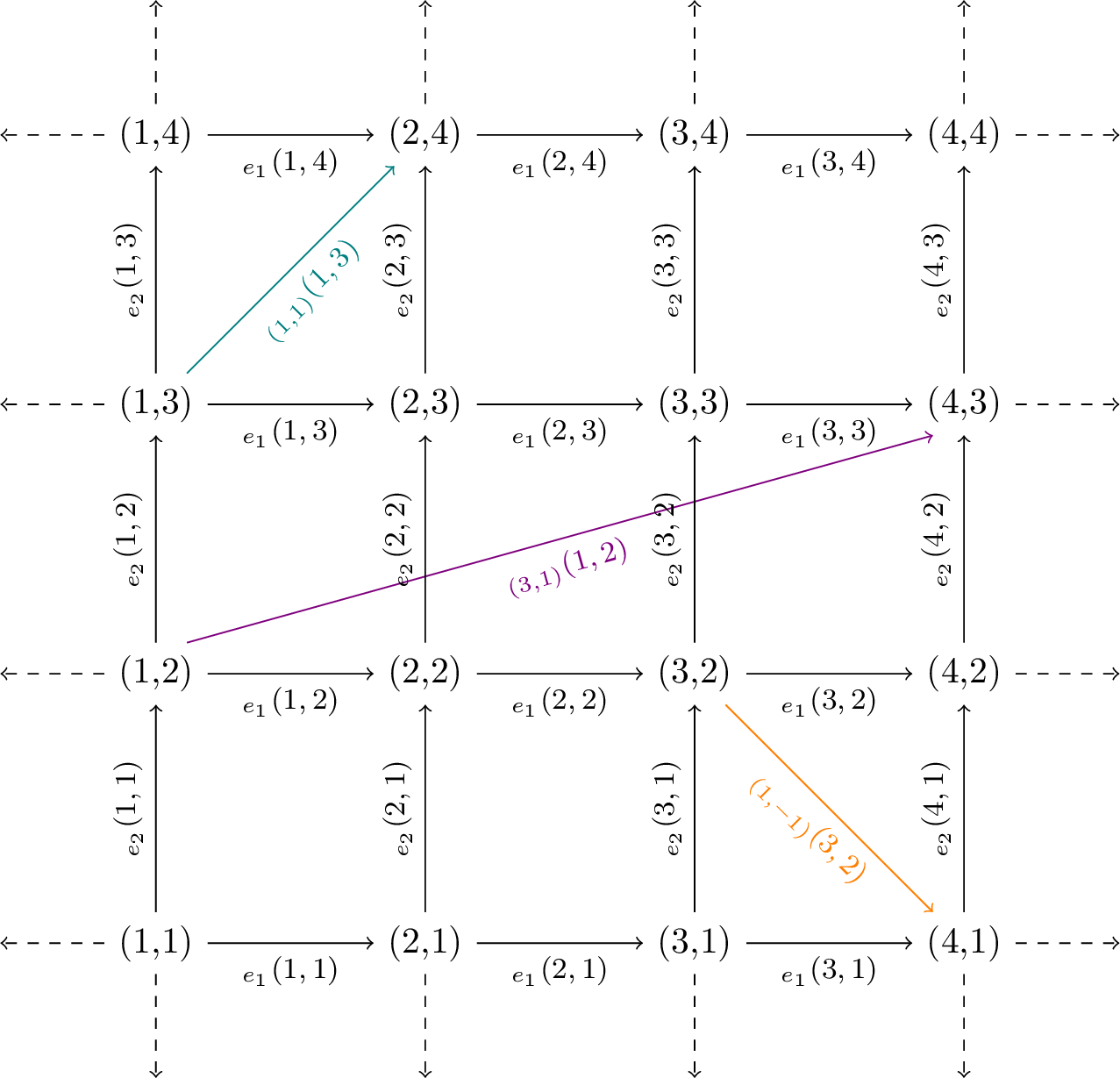
Example 8. Using the CMF defined in Example 4, We note that: \[\mathcal{M}_{(2,0)}(1,1) = \begin{pmatrix} -\frac{27}{8} & -\frac{35}{8} \\ \frac{243}{8} & \frac{251}{8} \\ \end{pmatrix}\quad \mathcal{M}_{(2,0)}(-2,0) = \begin{pmatrix} 0 & -1 \\ 0 & 1\\ \end{pmatrix}\notin\text{GL}_2(\mathbb{Q})\] However, \(\mathcal{M}_{(0,-1)}(1,1)\) is not defined.
It is useful to examine the matrices associated with straight paths in \(x+\mathbb{Z}^d\). We call such paths (starting at point \(x\) and moving by \(v\) at each step) trajectories, and the associated sequence of matrices trajectory matrices. A definition:
Definition 13. In a CMF \(\mathcal{M}\) of dimension \(d\) and rank \(r\) over \(K\), we define a trajectory matrix* \(T_{x,v}(n)\) as the matrix that is associated with the \(n\)th step (starting at 0) in the trajectory \(x+nv\) \[T_{x,v}(n) \mathrel{\vcenter{:}}= \mathcal{M}_v(x+nv)\in \text{GL}_r(K(n))\]*
Using 3 we have the following:
Remark 10. Defining \(\prod\) notation for matrices thusly: \[\prod_{k=0}^n M_k = M_0\cdot M_1\cdots M_n\] results in: \[\label{eq:prod95of95traj} \mathcal{M}_{nv}(x) = \prod_{k=0}^{n-1} T_{x,v}(k)\qquad{(2)}\]
Example 9. Using the CMF defined in Example 4, we see that: \[T_{(1,1),(1,0)}(n) = \begin{pmatrix}0 & -1\\\frac{\left(n + 2\right)^{3}}{\left(n + 1\right)^{3}} & \frac{\left(2 n + 3\right) \left(n^{2} + 3 n + 3\right)}{\left(n + 1\right)^{3}}\end{pmatrix}\] \[T_{(1,1),(1,1)}(n) = \begin{pmatrix}- \frac{\left(n + 2\right)^{3}}{\left(n + 1\right)^{3}} & \frac{\left(- 2 n - 3\right) \left(3 n^{2} + 9 n + 7\right)}{\left(n + 1\right)^{3}}\\\frac{6 \left(n + 2\right)^{3}}{\left(n + 1\right)^{3}} & \frac{35 n^{3} + 159 n^{2} + 243 n + 125}{\left(n + 1\right)^{3}}\end{pmatrix}\]
Remark 11. Note that from Example 6, trajectory matrices generate a 1-dimensional CMF. In fact, as 1-dimensional CMFs are very well studied (under the guise of D-finite systems), CMFs can be considered higher dimensional generalizations of D-finite systems.
A final preliminary notion that requires a definition is that of a coboundary transformation:
Definition 14. Two CMFs \(\mathcal{M}^1,\mathcal{M}^2\) of dimension \(d\) and rank \(r\) over \(K\), are coboundary equivalent* (which we notate as \(\mathcal{M}^1 \sim \mathcal{M}^2\)) if there exists a matrix \(A \in \text{GL}_r(K(\mathbf{x}))\) such
that \[A \cdot \mathcal{M}^1_v = \mathcal{M}^2_v \cdot \sigma_v(A)\] or equivalently: \[A \mathcal{M}^1_v S_v = \mathcal{M}^2_v S_v A\] for every \(v \in
\mathbb{Z}^d\).
The matrix \(A\) will be referred to as the *coboundary matrix**
It is a good exercise to verify that in fact a coboundary transformation \(\mathcal{M}_v\mapsto A^{-1}\cdot\mathcal{M}_v\cdot \sigma_v(A)\) satisfies the cocycle condition 1 . A few examples:
Example 10. The CMF from Example 4 is coboundary equivalent to the CMF generated by: \[\overline{M}_1 = \begin{pmatrix} \frac{x_{2} \left(2 x_{1} + 1\right) \left(x_{2} - 1\right) + \left(x_{1} + 1\right)^{3}}{x_{1}^{3}} & \frac{x_{2}^{2} \left(2 x_{1} + 1\right) \left(x_{2} - 1\right)}{x_{1}^{3}}\\\frac{x_{1}^{3} + x_{2} \left(2 x_{1} + 1\right) \left(x_{2} - 1\right) + \left(x_{1} + 1\right)^{3}}{x_{1}^{3} x_{2}} & \frac{x_{1}^{3} + x_{2} \left(2 x_{1} + 1\right) \left(x_{2} - 1\right)}{x_{1}^{3}} \end{pmatrix}\quad \overline{M}_2 = \begin{pmatrix} \frac{2 x_{1}^{2}}{x_{2}^{2}} + 1 & \frac{2 x_{1} \left(x_{2} + 1\right)}{x_{2}}\\\frac{2 x_{1} \left(x_{1}^{2} + x_{2}^{2}\right)}{x_{2}^{4}} & \frac{\left(2 x_{1}^{2} + x_{2}^{2}\right) \left(x_{2} + 1\right)}{x_{2}^{3}} \end{pmatrix}\] Via the coboundary matrix \(A = \begin{pmatrix} 1&-y\\ 1&y \end{pmatrix}\). This as: \[\overline{M}_1 = A^{-1}M_1\sigma_{1}(A)\quad\overline{M}_2 = A^{-1}M_2\sigma_{2}(A)\]
Example 11. If we define \(\overline{\mathcal{M}} \mathrel{\vcenter{:}}= \sigma_w(\mathcal{M})\), then \(\overline{\mathcal{M}} \sim \mathcal{M}\). This as for \(A = \mathcal{M}_w\): \[A\overline{\mathcal{M}}_v = \mathcal{M}_w \sigma_w(\mathcal{M}_v) = \mathcal{M}_{v+w} = \mathcal{M}_v\sigma_v(\mathcal{M}_w) =\mathcal{M}_v\sigma_v(A)\]
Example 12. Note how coboundary transforms effect trajectory matrices. Recall the trajectory matrices calculated in Example 9 Using the coboundary matrix \(A = \begin{pmatrix} \frac{1}{x_{1}^{3}} & - \frac{1}{x_{2}^{3}}\\0 & \frac{x_{1}^{3} + 2 x_{1}^{2} x_{2} + 2 x_{1} x_{2}^{2} + x_{2}^{3}}{x_{1}^{3} x_{2}^{3}} \end{pmatrix}\) on the CMF from Example 4 , one gets that the trajectory matrix of the coboundary CMF \(\overline{\mathcal{M}}\) is: \[\overline{T}_{(1,1),(1,1)}(n) = \begin{pmatrix} 0 & - \frac{\left(n + 1\right)^{3}}{\left(n + 2\right)^{3}}\\1 & \frac{\left(2 n + 3\right) \left(17 n^{2} + 51 n + 39\right)}{\left(n + 2\right)^{3}} \end{pmatrix}\] Note that this matrix is in companion form, and encodes the recurrence: \[(n+2)^3u(n+2)-(2n+3)(17n^2+51n+39)u(n+1) +(n+1)^3 u(n) = 0\] The recurrence used in Apérys proof of the irrationality of \(\zeta(3)\) (see Theorem 3).
Finally, there are the notions of Dual CMFs, and Sub-CMFs. These are described in Appendix 6
3 CMF construction using D-finite functions↩︎
Other discussions of conservative matrix fields [[20]][16][[21]][19] highlight their utility in unifying approximations of constants, combinatorial identity proofs, and irrationality proofs. However, save the last reference, these only discuss CMFs of rank \(r=2\). In this section, we will demonstrate a construction of non-trivial conservative matrix fields of general dimension and rank, using D-finite functions. Consider a D-finite function \(f(\boldsymbol{x},\boldsymbol{z})\in F\). As discussed in Remark 3, the image of \(f\) under the Ore algebra \(\mathbb{A}'\) will be finite dimensional. Say \(\dim_{K(\boldsymbol{x},\boldsymbol{z})} \mathbb{A}'.f = r\). Then given a basis \(B = (b_1.f,\dots,b_r.f),b_i\in\mathbb{A}'\) of \(\mathbb{A}'.f\) over \(K(\boldsymbol{x},\boldsymbol{z})\), any element of the image is a \(K(\boldsymbol{x},\boldsymbol{z})\) - linear combination of \((b_1.f,\dots,b_r.f)\).
Remark 12. \({}\)
For \(L\in \mathbb{A}'\), the coordinates of \(L.f\) in the basis \(B\) can be calculated using an appropriate Gröbner basis.
\(\sigma_v(B)\) is also a basis for \(\mathbb{A}'.f\), from the invertibility of \(\sigma_v\) as action on \(F\)
Definition 15. Consider a D-finite function \(f(\boldsymbol{x},\boldsymbol{z})\in F\), and a basis \(B = (b_1.f,\dots,b_r.f),b_i\in\mathbb{A}'\) for \(\mathbb{A}'.f\).
Then, the basis change matrix* \(\mathcal{M}^f_{v}\) is the matrix that maps \(B\mapsto S_{v}. B\). Meaning the unique matrix \(\mathcal{M}^f_v\in
\text{GL}_r(K(\boldsymbol{x},\boldsymbol{z}))\), satisfying: \[\label{eq:Dfin32Basis32Change} (b_1.f,\dots,b_r.f)\cdot \mathcal{M}^f_v =(S_{v}b_1.f,\dots,S_{v}b_r.f) =
\sigma_v((b_1.f,\dots,b_r.f))\tag{4}\] *
Theorem 6. Given a D-finite function \(f(\boldsymbol{x},\boldsymbol{z})\in F\) , with an image of dimension \(\dim(\mathbb{A}.f) = r\), and some basis \(B\) of the image, the basis changing matrices \(\mathcal{M}^f_v\) constitute a CMF of dimension \(d\), rank \(r\), over the field \(K(\boldsymbol{z})\).
Proof. Let us show that \(\mathcal{M}^f_v\) satisfy the cocycle condition 1 . It suffices to demonstrate that \[\sigma_{v+w}(B) = B\cdot \mathcal{M}^f_{v+w} = B\cdot \mathcal{M}^f_{v}\cdot \sigma_v(\mathcal{M}^f_{w})\] From \(B\) being a basis. And indeed: \[B\cdot \mathcal{M}^f_{v}\cdot \sigma_v(\mathcal{M}^f_{w}) = \sigma_v(B)\cdot \sigma_v(\mathcal{M}^f_{w})= \sigma_v(B\cdot \mathcal{M}^f_{w}) = \sigma_{v+w}(B)\] ◻
This construction is fundamental to understanding CMFs and reveals them to be natural mathematical objects. Note for example how coboundary equivalence translates to a change of basis \(B\):
Proposition 7. a CMF \(\mathcal{M}\) is coboundary to a CMF generated by a D-finite function \(f\) (i.e. \(\mathcal{M}\sim\mathcal{M}^f\)) if and only if \(\mathcal{M}\) can also be generated by \(f\).
Proof. First, it is demonstrated that the choice of the basis \(B\) of \(\mathbb{A}'.f\) gives coboundary CMFs. Say both \(B,B'\) are
bases of \(\mathbb{A}'.f\), and their appropriate CMFs are \(\mathcal{M}^{f} , {\mathcal{M}^{f}}{}'\). Then if \(A\) is the basis change matrix:
\[(b_1.f,\dots,b_r.f)\cdot A = (b_1'.f,\dots,b_r'.f)\] then we have: \[(b_1.f,\dots,b_r.f)\cdot A \cdot {\mathcal{M}_v^{f}}{}'= (b_1'.f,\dots,b_r'.f)\cdot
{\mathcal{M}_v^{f}}{}' =\sigma_v(B') =\] \[=\sigma_v(BA^{-1}) = (b_1.f,\dots,b_r.f)\cdot\mathcal{M}_v^f\cdot \sigma_v(A^{-1})\] Thus: \[A \cdot
{\mathcal{M}_v^{f}}{}'=\mathcal{M}_v^f\cdot \sigma_v(A^{-1})\iff \mathcal{M}^{f}\sim{\mathcal{M}^{f}}{}'\] This implies CMFs generated by the same function are coboundary.
The converse is true by defining \(B'\mathrel{\vcenter{:}}= B\cdot A\), with \(A\) the coboundary matrix of the equivalence \(\mathcal{M}\sim\mathcal{M}^f\). ◻
CMFs can also be thought of as gauge transformations:
Definition 16. For \(f(\boldsymbol{x},\boldsymbol{z})\) D-finite and \(B\) basis of \(\mathbb{A}'.f\), we shall define \(\mathcal{M}_{\theta_{z_i}}^f\in M_{r\times r}(K(\boldsymbol{x},\boldsymbol{z}))\) as the matrix satisfying: \[(b_1.f,\dots,b_r.f)\mathcal{M}_{\theta_{z_i}}^f = (\theta_{z_i}b_1.f,\dots,\theta_{z_i}b_r.f)\]
Lemma 1. For all \(v\in\mathbb{Z}^d\), \(\mathcal{M}_v^f\) is a gauge transformation matrix of the system \(\theta_{z_i}.g = g\cdot\mathcal{M}_{\theta_{z_i}}^f\) to the system \(\theta_{z_i}.g=g\cdot \sigma_v(\mathcal{M}_{\theta_{z_i}}^f)\)
Proof. We must show that \(\mathcal{M}_v^f\sigma_v(\mathcal{M}^f_{\theta_{z_i}}) = \theta_{z_i}.\mathcal{M}^f_v+\mathcal{M}^f_{\theta_{z_i}}\mathcal{M}^f_v\). That can be verified by checking how both sides act on \(B\): \[(b_1.f,\dots,b_r.f)\cdot\mathcal{M}_v^f\sigma_v(\mathcal{M}^f_{\theta_{z_i}}) = \sigma_v((b_1.f,\dots,b_r.f)\cdot\mathcal{M}^f_{\theta_{z_i}} )= (S_v\theta_{z_i}b_1.f,\dots,S_v\theta_{z_i}b_r.f)\] \[(b_1.f,\dots,b_r.f)\cdot (\theta_{z_i}.\mathcal{M}^f_v+\mathcal{M}^f_{\theta_{z_i}}\mathcal{M}^f_v) = (b_1.f,\dots,b_r.f)\cdot \theta_{z_i}.\mathcal{M}^f_v+(\theta_{z_i}b_1.f,\dots,\theta_{z_i}b_r.f)\cdot\mathcal{M}^f_v=\] \[=\theta_{z_i}.\left((b_1.f,\dots,b_r.f)\cdot \mathcal{M}^f_v\right) = (S_v\theta_{z_i}b_1.f,\dots,S_v\theta_{z_i}b_r.f)\] Giving the desired equality. ◻
Example 13. Consider Tricomi’s function \(U(x_1,x_2,z)\), which is often used in physics [31]. It is D-finite, and in \(\mathbb{A}= \mathbb{Q}(x_1,x_2,z)[S_{x_1},S_{x_2}]\), its annihilator is: \[\text{ann} (U) = \langle z S_{x_2}+\left(x_1^2-x_2 x_1+x_1\right) S_{x_1}+\left(-x_1-z\right),z S_{x_2}^2+S_{x_2} \left(-x_2-z\right)+\left(x_2-x_1\right)\rangle\]
Thus, if we select \(B = (U,S_{x_2}.U)\), we can calculate the generators of \(\mathcal{M}^U\): \[S_{x_2}.B = (S_{x_2}.U,S_{x_2}^2.U)=
(U,S_{x_2}.U)\begin{pmatrix} 0&\frac{x_1-x_2}{z}\\ 1&\frac{x_2+z}{z}
\end{pmatrix} = B\cdot \mathcal{M}^U_{(0,1)}\] \[S_{x_1}.B = (S_{x_1}.U,S_{x_1}S_{x_2}.U)= (U,S_{x_2}.U)\begin{pmatrix} \frac{x_1+z}{x_1^2-x_2 x_1+x_1}&-\frac{1}{x_1}\\ \frac{-z}{x_1^2-x_2 x_1+x_1}&\frac{1}{x_1}
\end{pmatrix} = B\cdot \mathcal{M}^U_{(1,0)}\] Hence, \(\mathcal{M}^U\) is a conservative matrix field of dimension \(2\), rank \(2\), over field
\(\mathbb{Q}(z)\).
Furthermore, \(U\) satisfies: \[\theta_z.U(x_1,x_2,z) = z(U(x_1,x_2,z)-U(x_1,x_2+1,z))\] Implying that for the extended algebra \(\mathbb{A}=
\mathbb{Q}(x_1,x_2,z)[S_{x_1},S_{x_2},\theta_z]\) we have: \[\theta_z\equiv z-zS_{x_2} \mod \text{ann}(U)\quad\text{or}\quad\theta_z.U = (z-zS_{x_2}).U\] Hence, from linearity, the matrix \(\mathcal{M}^U_{\theta_z}\) is: \[\mathcal{M}^U_{\theta_z} = zI-z\mathcal{M}^U_{(0,1)} = \begin{pmatrix} z&x_2-x_1\\ -z&-x_2
\end{pmatrix}\]
Example 14. Consider the binomial function: \(f(x_1,x_2) =\binom{x_1}{x_2}\). This is a D-finite function, with the following annihilator: \[\text{ann}(f) = \langle(1+x_1-x_2)S_{x_1}-(1+x_1),(1+x_2)S_{x_2}-(x_1-x_2)\rangle\] The dimension \(\dim \mathbb{A}'.f = 1\), thus with \(B = (f)\), we have: \(\mathcal{M}^f_{(1,0)} = 1+\frac{x_2}{1+x_1-x_2},\mathcal{M}^f_{(0,1)} = \frac{x_1-x_2}{1+x_2}\). Thus \(\mathcal{M}^f\) is a conservative matrix field of dimension \(2\), rank \(1\), over field \(\mathbb{Q}\) (Also known as a multivariate hypergeometric term, see Remark 9).
A highly useful such CMF is generated by the generalized hypergeometric function \(_pF_q\).
In the case \(z\notin\left\{ 0,1 \right\}\), the annihilator of \(\begingroup \pFqmuskip=8mu\relax \mathcode`\,=\string"8000 \begingroup\lccode`\~=`\,
\lowercase{\endgroup\let~}\mskip\pFqmuskip {}_{p}F_{q}{\left[\genfrac..{0pt}{}{x_1,\dots,x_p}{x_{p+1},\dots,x_{p+q}};z\right]} \endgroup\) is generated by its ODE, and its contiguous relations: \[\label{eq:Cont32Rel} \text{ann}\left( \begingroup \pFqmuskip=8mu\relax \mathcode`\,=\string"8000 \begingroup\lccode`\~=`\, \lowercase{\endgroup\let~}\mskip\pFqmuskip
{}_{p}F_{q}{\left[\genfrac..{0pt}{}{x_1,\dots,x_p}{x_{p+1},\dots,x_{p+q}};z\right]} \endgroup
\right) = \langle\sum_{k=0}^{r}t_k(\boldsymbol{x},z)\theta_z^k,\frac{\theta_z}{x_i}+1-S_{e_i},\frac{\theta_z}{y_j-1}+1-S_{-e_{p+j}}\rangle\tag{5}\] with \(r = \max(p,q+1)\) the order of the differential
equation, and \(t_k\in\mathbb{Q}(\boldsymbol{x},z),t_{r} = 1\). If we select our basis \(B\) to be \(({}_pF_q,\theta_z
.{}_pF_q,\theta_z^2.{}_pF_q,\dots,\theta_z^{r-1}.{}_pF_q)\) then \(\mathcal{M}^{{}_pF_q}_{\theta_z}\) is in companion form: \[\mathcal{M}^{{}_pF_q}_{\theta_z} = \begin{pmatrix}
0 & 0 & \cdots & 0 & -t_0(\mathbf{x}, z) \\
1 & 0 & \cdots & 0 & -t_1(\mathbf{x}, z) \\
0 & 1 & \cdots & 0 & -t_2(\mathbf{x}, z) \\
\vdots & \vdots & \ddots & \vdots & \vdots \\
0 & 0 & \cdots & 1 & -t_{r-1}(\mathbf{x}, z)
\end{pmatrix}\] and directly from the contiguous relations in 5 , one gets: \[\label{eq:pFq32CMF} \forall_{1\leq i\leq p}\mathcal{M}^{{}_pF_q}_{e_i}
=\frac{1}{x_i}\mathcal{M}^{{}_pF_q}_{\theta_z}+I\;, \;\forall_{p+1\leq j\leq p+q}\mathcal{M}^{{}_pF_q}_{-e_j}=\frac{1}{x_j-1}\mathcal{M}^{{}_pF_q}_{\theta_z}+I.\tag{6}\]
Example 15. Let us construct the CMF for \(\begingroup \pFqmuskip=8mu\relax \mathcode`\,=\string"8000 \begingroup\lccode`\~=`\, \lowercase{\endgroup\let~}\mskip\pFqmuskip {}_{2}F_{1}{\left[\genfrac..{0pt}{}{x_1,x_2}{x_3};z\right]} \endgroup\). First, note \(r = 2\). The differential equation is: \[(1-z)\theta_z^2 . \begingroup \pFqmuskip=8mu\relax \mathcode`\,=\string"8000 \begingroup\lccode`\~=`\, \lowercase{\endgroup\let~}\mskip\pFqmuskip {}_{2}F_{1}{\left[\genfrac..{0pt}{}{x_1,x_2}{x_3};z\right]} \endgroup = x_1x_2z \begingroup \pFqmuskip=8mu\relax \mathcode`\,=\string"8000 \begingroup\lccode`\~=`\, \lowercase{\endgroup\let~}\mskip\pFqmuskip {}_{2}F_{1}{\left[\genfrac..{0pt}{}{x_1,x_2}{x_3};z\right]} \endgroup +((x_1+x_2)z+1-x_3)\theta_z. \begingroup \pFqmuskip=8mu\relax \mathcode`\,=\string"8000 \begingroup\lccode`\~=`\, \lowercase{\endgroup\let~}\mskip\pFqmuskip {}_{2}F_{1}{\left[\genfrac..{0pt}{}{x_1,x_2}{x_3};z\right]} \endgroup\] Meaning, setting \(B = ({}_2F_1,\theta_z.{}_2F_1)\), we get: \[\mathcal{M}^{{}_2F_1}_{\theta_z} = \begin{pmatrix} 0 & \frac{x_1 x_2 z}{1-z} \\ 1 & \frac{x_1 z+x_2 z-x_3+1}{1-z} \\ \end{pmatrix}\] Giving the generators of \(\mathcal{M}^{{}_2F_1}\) using 6 : \[\mathcal{M}^{{}_2F_1}_{e_1} = \begin{pmatrix} 1 & \frac{x_2 z}{1-z} \\ \frac{1}{x_1} & \frac{x_1+x_2 z-x_3+1}{x_1(1-z)} \\ \end{pmatrix}\quad \mathcal{M}^{{}_2F_1}_{e_2} = \begin{pmatrix} 1 & \frac{x_1 z}{1-z} \\ \frac{1}{x_2} & \frac{x_1 z+x_2-x_3+1}{x_2(1-z)} \\ \end{pmatrix}\]\[\mathcal{M}^{{}_2F_1}_{e_3} = \sigma_3(\mathcal{M}^{{}_2F_1}_{-e_3})^{-1} = \sigma_3\left(\frac{1}{x_3-1}\mathcal{M}^{{}_pF_q}_{\theta_z}+I \right)^{-1}= \frac{x_3}{(x_1-x_3)(x_2-x_3)}\begin{pmatrix} -x_1-x_2+x_3 & x_1 x_2 \\ \frac{1}{z}-1 & \frac{x_3 (z-1)}{z} \\ \end{pmatrix}.\] Note that this is the CMF from Example 5
4 CMF Ratios, and CMF Limits↩︎
This section will define CMF limits, and CMF ratios, which are generalizations of Apéry limits and D-finite ratios. The remainder of this document will discuss, both phenomenologically and rigorously, the properties and relations of CMF ratios.
Definition 17. Let \(\mathcal{M}\) be a CMF of dimension \(d\) rank \(r\) over \(\mathbb{Q}\).
Select a trajectory \(x+nv\) such that \(v\in\mathbb{Z}^d,x\in\mathbb{Q}^d\), and four vectors \(p,p',q,q'\in \mathbb{Q}^r\).
Then, the CMF Ratio* is defined as the following sequence: \[\label{eq:CMF95limit95def} \mathcal{L}_{x,v}^{p,p',q,q'}(n) \mathrel{\vcenter{:}}= \frac{p^t\cdot
\mathcal{M}_{nv}(x)\cdot p'}{q^t\cdot \mathcal{M}_{nv}(x)\cdot q'}.\tag{7}\] For brevity, denote \(\mathcal{L}_{x,v}^{p,q}\mathrel{\vcenter{:}}=\mathcal{L}_{x,v}^{p,e_r,q,e_r}\). The ratio \(\mathcal{L}_{x,v}^{p,q}\) can also be thought of as a ratio of the inner products of \(p\) and \(q\) with the last column of \(\mathcal{M}_{nv}(x)\). Finally, the limit of \(\mathcal{L}_{x,v}^{p,p',q,q'}(n)\) is called a CMF Limit.*
Example 16. Consider the CMF generated by \(\begingroup \pFqmuskip=8mu\relax \mathcode`\,=\string"8000 \begingroup\lccode`\~=`\, \lowercase{\endgroup\let~}\mskip\pFqmuskip
{}_{2}F_{1}{\left[\genfrac..{0pt}{}{x_1,x_2}{x_3};-1\right]} \endgroup\). This CMF can be obtained from the CMF detailed in Examples 5,15, if one substitutes \(z=-1\). Let us calculate and graph a few of its CMF ratios:
First: \(\mathcal{L}_{x,v}^{p,q}(n)\) for \(x = v = (1,1,2),p = (0,1),q = (-2,2)\). Let us first calculate \(\mathcal{M}_{nv}(x)\) for a few values of \(n\): \[\mathcal{M}_0(x) = I, \mathcal{M}_v(x) = \begin{pmatrix} -6&18\\-24&66
\end{pmatrix},\mathcal{M}_{2v}(x) = \begin{pmatrix} -150&660\\-540&2370
\end{pmatrix}, \mathcal{M}_{3v}(x) =\begin{pmatrix} - \frac{10220}{3} & \frac{62300}{3}\\- \frac{36680}{3} & \frac{223580}{3}
\end{pmatrix}.\] Hence: \[\mathcal{L}_{x,v}^{p,q}(0) = \frac{1}{2},\mathcal{L}_{x,v}^{p,q}(1) = \frac{11}{16},\mathcal{L}_{x,v}^{p,q}(2) = \frac{79}{114},\mathcal{L}_{x,v}^{p,q}(3) = \frac{1597}{2304}.\] Or in
decimal form: \[\mathcal{L}_{x,v}^{p,q}(n) = (0.5,0.6875,0.6930\dots,0.69314\dots,\dots)\] The sequence appears to converge to \(\log(2)\approx0.693147\dots\). Moreover, it has a
non-trivial convergence rate \(\rho = -3.53\dots\) and seems to have a non trivial and positive (!) irrationality measure \(\delta \approx 0.31\).
In contrast, consider the CMF ratio \(\mathcal{L}_{x,v}^{p,q}(n)\) for \(x = v = (-1,-1,2),p = (0,1),q = (-2,2)\). The first few values are: \[\mathcal{L}_{x,v}^{p,q}(n) = (\frac{1}{2},\frac{19}{60}, \frac{1109}{5460},\frac{713}{13860},- \frac{327713}{540540},\dots)\] This sequence does not seem to converge. The first 300 values of this sequence are plotted in Figure
2

It is useful to consider \(\mathcal{L}_{x,v}^{p,q}(n)\) where \(T_{x,v}(n)\) is in companion form, and later, to compare CMF ratios of coboundary equivalent CMFs.
Proposition 8. If \(T_{x,v}(n)\) is in companion form and the CMF Ratio \(\mathcal{L}_{x,v}^{p,q}(n)\) converges, then it is a D-finite ratio (implying the CMF limit is an Apéry limit).
Proof. Given ?? , for a trajectory matrix in companion form, the last column of \(\mathcal{M}_{nv}(x)\) contains the solutions to the recursion contained in \(T_{x,v}(n)\), with initial conditions \(e_1,\dots,e_r\). Thus, \(p^t\cdot \mathcal{M}_{nv}(x)\cdot e_r\) is the solution with initial condition \(p\in \mathbb{Q}^r\), making \(\mathcal{L}_{x,v}^{p,q}\) a D-finite ratio. ◻
Corollary 3. Any D-finite ratio is a CMF ratio (i.e., any Apéry limit is a CMF limit)
Proof. Let \(u_p(n)\) and \(u_q(n)\) be solutions to a minimal recursion \(L\in \mathbb{Q}(n)[S_n]\) of order \(r\), with initial conditions \(p\) and \(q\) respectively. Then, we can calculate the companion matrix \(M(n)\in\text{GL}_r(\mathbb{Q}(n))\) encoding \(L\). The matrix \(M(n)\) generates a CMF of dimension \(1\) and rank \(r\) (see Example 6), such that the trajectory matrix \(T_{0,1}(n) = M(n)\). Thus, the generated CMF has a CMF ratio \(\mathcal{L}^{p,q}_{0,1}(n)\) which is equal to the desired D-finite ratio. ◻
Proposition 9. Suppose for a CMF \(\mathcal{M}\), the trajectory matrix \(T_{x,v}(n)\) is in companion form. Suppose further, that the recurrence operator \(L\) encoded by \(T_{x,v}(n)\) satisfies the conditions of Poincaré and Perron, and is irreducible (in the sense of definition 2 in [32]).
Then, for any \(a(n)\in\mathbb{Q}(n)^r\), and any \(p,q\) such that \(\mathcal{L}_{x,v}^{p,q}(n)\) converges, \(\lim_{n\to\infty}
\mathcal{L}_{x,v}^{p,a(n),q,a(n)}(n) = \lim_{n\to\infty} \mathcal{L}_{x,v}^{p,q}(n)\). Furthermore, both have the same convergence rate.
Proof. This case is similar to the proof above of Proposition 8, but instead of a simple ratio of solutions \(\mathcal{L}_{x,v}^{p,q}(n) = \frac{u_p(n)}{u_q(n)}\), we have \(\mathcal{L}_{x,v}^{p,a(n),q,a(n)}(n) = \frac{\sum_{i=1}^{r} a_i(n)u_p(n-(i-1))}{\sum_{i=1}^{r} a_i(n)u_q(n-(i-1))}\). From Poincaré–Perron, we have: \[\sum_{i=1}^{r} a_i(n)u_p(n-(i-1)) = \sum_{j=1}^r c_j \sum_{i=1}^{r} a_i(n)\lambda_j^{n-(i-1)}f_j(n-(i-1)).\] Notice that the irreducibility of \(L\) implies \(\sum_{i=1}^{r} a_i(n)\lambda_j^{n-(i-1)}f_j(n-(i-1))\neq0\), as that would imply the solution \(\lambda_j^nf_j(n)\) has a smaller annihilator. This implies that if we define: \[g_j(n) \mathrel{\vcenter{:}}= \sum_{i=1}^{r} a_i(n)\lambda_j^{-(i-1)}f_j(n-(i-1))\] then \(\frac{f_j(n+1)}{f_j(n)}\to1\implies\frac{g_j(n+1)}{g_j(n)}\to1\). This along with: \[\sum_{i=1}^{r} a_i(n)u_p(n-(i-1)) = \sum_{i=1}^{r} c_i\lambda_i^ng_i(n)\] gives exactly the same setup for the proof of Proposition 4. Thus giving that: \[\lim_{n\to\infty} \mathcal{L}_{x,v}^{p,a(n),q,a(n)}(n) = \frac{c_j}{\tilde{c_j}} = \lim_{n\to\infty} \frac{u_p(n)}{u_q(n)}=\lim_{n\to\infty} \mathcal{L}_{x,v}^{p,q}(n)\] \[\rho = \log\left| \frac{\lambda_k}{\lambda_j} \right|\] with \(j,k\) defined as in Proposition 4 ◻
In most cases, trajectory matrices are not in companion form. Thus, let us examine the effect of coboundary equivalence on CMF ratios and limits:
Proposition 10. For two coboundary CMFs \(\mathcal{M}\sim \overline{\mathcal{M}}\;, \;\mathcal{M}_v =A\overline{\mathcal{M}_v}\sigma_v(A^{-1})\), with resulting ratios \(\mathcal{L},\overline{\mathcal{L}}\) respectively, then: \[\mathcal{L}_{x,v}^{p,p',q,q'}(n) =\overline{\mathcal{L}}_{x,v}^{A^t(x)p,A^{-1}(x+nv)p',A^t(x)q,A^{-1}(x+nv)q'}(n)\]
Proof. \[\mathcal{L}_{x,v}^{p,p',q,q'}(n) = \frac{p^t\cdot \mathcal{M}_{nv}(x)\cdot p'}{q^t\cdot \mathcal{M}_{nv}(x)\cdot q'} = \frac{p^t\cdot [A\overline{\mathcal{M}}_{nv}\sigma_{nv}(A^{-1})](x)\cdot p'}{q^t\cdot [A\overline{\mathcal{M}}_{nv}\sigma_{nv}(A^{-1})](x)\cdot q'} =\] \[=\frac{p^t\cdot A(x)\overline{\mathcal{M}}_{nv}(x)A^{-1}(x+nv)\cdot p'}{q^t\cdot A(x)\overline{\mathcal{M}}_{nv}(x)A^{-1}(x+nv)\cdot q'} =\overline{\mathcal{L}}_{x,v}^{A^t(x)p,A^{-1}(x+nv)p',A^t(x)q,A^{-1}(x+nv)q'}(n)\] ◻
Corollary 4. for a CMF \(\mathcal{M}\), and its ratio \(\mathcal{L}\), if, for certain \(x,v\), there exists \(A\in\text{GL}_r(\mathbb{Q}(\boldsymbol{x}))\) s.t \(C(n)\mathrel{\vcenter{:}}= A(x+(n-1)v)T_{x,v}(n)A^{-1}(x+nv)\) is in companion form, and encodes an irreducible Poincaré-Perron recurrence \(L\), then \(\mathcal{L}_{x,v}^{p,q}(n)\) has the same limit, and the same convergence rate, as the D-finite ratio of \(L\), with initial values \(A^t(x)p,A^t(x)q\)
Proof. The coboundary transform \(A\) connecting \(C(n)\) and \(T_{x,v}(n)\) implies that for \(\mathcal{M}\sim \overline{\mathcal{M}}\;, \;\mathcal{M}_v =A\overline{\mathcal{M}_v}\sigma_v(A^{-1})\), we have that the trajectory matrix \(\overline{T}_{x,v}(n) = C(n)\), as required in Proposition 9. Thus, from Proposition 10 \[\mathcal{L}_{x,v}^{p,q}(n) =\overline{\mathcal{L}}_{x,v}^{A^t(x)p,A^{-1}(x+nv)e_r,A^t(x)q,A^{-1}(x+nv)e_r}(n)\] Which has the same limit and convergence rate as \(\frac{u_{A^t(x)p}(n)}{u_{A^t(x)q}(n)}\) ◻
Example 17. Recall Example 12. There, a coboundary matrix is provided, that connects the companion matrix of Apéry’s recurrence \(L\), with the trajectory matrix \(T_{(1,1),(1,1)}(n)\) and satisfies Corollary 4. Thus, we know that \(\mathcal{L}_{(1,1),(1,1)}^{(0,1),(1,1)}(n)\) converges to and has the same convergence rate as the D-finite ratio of \(L\), with initial values \(A^t(x)p,A^t(x)q\). As \(A^t(1,1) = \begin{pmatrix}1 & 0\\-1 & 6\end{pmatrix}\) we have the initial conditions: \[u_1(0) = 0, u_1(1) = 6, u_2(0) = 1, u_2(1) = 5\] Exactly as in Theorem 3. Thus \(\mathcal{L}_{(1,1),(1,1)}^{(0,1),(1,1)}(n)\) converges to \(\zeta(3)\), with convergence rate \(\rho = -8\log(\sqrt{2}+1)\). In fact, it can also be shown it is similarly bounded in height. This exemplifies an empirical observation: the irrationality measure \(\delta\) for the CMF ratio in Corollary 4 is identical to that of the corresponding D-finite ratio. This phenomena is used extensively in [21].
Summarizing, the above demonstrates that CMF ratios and limits, a higher dimensional generalization of D-finite ratios and Apéry limits, inherit their useful properties in Proposition 4, at least under some reasonable assumptions. The following section will demonstrate some phenomenological properties of specific CMFs and CMF limits, formulate them into conjectures, prove some special cases, and suggest some applications and corollaries.
5 Experimental Analysis of Conservative Matrix Fields↩︎
The previous section demonstrates how to construct a sequence \(\mathcal{L}^{p,q}_{x,v}(n)\), with similar properties to D-finite ratios. One can analyze the behavior of the limit and the convergence of these sequences when changing the parameters \(x,v,p,q\). This section will focus on variations in the direction \(v\). First, one can note how they are effected by scaling: \(v\to kv\) for \(k\in\mathbb{N}\setminus\left\{ 0 \right\}\):
Remark 13. For a CMF ratio \(\mathcal{L}^{p,q}_{x,v}(n)\) that converges to \(l\) with non-trivial convergence rate \(\rho<0\),
the CMF ratio \(\mathcal{L}^{p,q}_{x,kv}(n),k\in\mathbb{N}\setminus\left\{ 0 \right\}\) has the same limit \(l\), and a convergence rate of \(k\rho\). If
furthermore \(\mathcal{L}^{p,q}_{x,v}(n)\) has a non-trivial irrationality measure \(\delta>-1\), then \(\mathcal{L}^{p,q}_{x,kv}(n)\) has the same
irrationality measure.
Suppose additionally \(T_{x,v}(n)\) is coboundary equivalent to an irreducible Poincaré-Perron recurrence \(L\), with eigenvalues \((\lambda_1,\dots,\lambda_r)\). then \(T_{kx,v}(n)\) is coboundary equivalent to a Poincaré-Perron recurrence \(L'\), with eigenvalues \((\lambda_1^k,\dots,\lambda_r^k)\).
Proof. As \(\mathcal{L}^{p,q}_{x,kv}(n)\) is a sub-sequence of \(\mathcal{L}^{p,q}_{x,v}(n)\), the first two points are an immediate corollary of Remark 8. The final point is clear as the conditions on \(L\) imply \(\exists \sum_{i=0}^r a_i(n)S_n^{ki}\in\langle L\rangle\). Defining \(L' \mathrel{\vcenter{:}}= \sum_{i=0}^r a_i(n)S_n^{i}\), implies for any solution \(u(n)\) of \(L\), that \(u(kn)\) is a solution of \(L'\). This demonstrates that \(L'\) has the desired eigenvalues. One can construct a basis changing matrix from \((u(n),u(n+1),\dots,u(n+r-1))\) to \((u(n),u(n+k),\dots,u(n+k(r-1)))\), which will provide a coboundary transform between \(T_{x,kv}(n)\) and the companion matrix of \(L'\). ◻
Hence, under some assumptions of existence, the limit, \(\delta\), \(\rho\), \(\eta\) and \(\log\left| \lambda_i \right|\) of \(\mathcal{L}^{p,q}_{x,v}(n)\) are homogeneous as functions of \(v\). The limit and irrationality measures are 0-homogeneous, and the convergence rate, height and \(\log\left| \lambda_i \right|\) are 1-homogeneous. This implies these quantities depend mostly on direction in \(\mathbb{Z}^d\). This observation suggests the analysis of the quantities \(l,\delta,\frac{\rho}{\left| v \right|},\frac{\log\left| \lambda_i \right|}{\left| v \right|}\) as functions of the direction of \(v\). We will select specific CMFs and parameters \(x,p,q\), and graph empirical evaluations of these quantities. We will sample \(v\) from a set of lattice points in \(\mathbb{Z}^d\cap B(0,R)\), for which \(\forall_{n\in\mathbb{N}}\;\mathcal{M}_{nv}(x)\in\text{GL}_r(\mathbb{Q})\). While \(\frac{\log\left| \lambda_i \right|}{\left| v \right|}\) can be calculated in closed form, the other parameters must be approximated. This will be done by evaluating late elements in the sequence, \(\mathcal{L}^{p,q}_{x,v}(n)\). for \(N \gg 1\): \[\hat{l} = \mathcal{L}^{p,q}_{x,v}(N)\approx\lim_{n\to\infty}\mathcal{L}^{p,q}_{x,v}(n)=l\quad \hat{\rho} =\frac{\log\left| \mathcal{L}^{p,q}_{x,v}(N)-\mathcal{L}^{p,q}_{x,v}(2N) \right|}{N} \approx\rho\] \[\hat{\delta} = -1-\frac{\log\left| \mathcal{L}^{p,q}_{x,v}(N)-\mathcal{L}^{p,q}_{x,v}(2N) \right|}{\log\left| H(\mathcal{L}^{p,q}_{x,v}(N)) \right|}\approx \delta\] These approximations are appropriate as \(\mathcal{L}^{p,q}_{x,v}(N) \approx l\pm e^{N\rho}\), implying:
\[\frac{\log\left| \mathcal{L}^{p,q}_{x,v}(N)-\mathcal{L}^{p,q}_{x,v}(2N) \right|}{N}\approx\frac{1}{N} \log\left| e^{N\rho}\pm e^{2N\rho} \right| =\] \[=\log\left| e^\rho \right|+\frac{1}{N}\log\left| 1\pm e^{N\rho} \right|\approx \rho\pm \frac{e^{N\rho}}{N}\approx \rho\] and the rest follow.
First, we will examine the CMF detailed in Example 4. It is generated by: \[M_{1} = \begin{pmatrix}0 & -1\\\frac{\left(x_{1} +
1\right)^{3}}{x_{1}^{3}} & \frac{x_{1}^{3} + 2 x_{2} \left(2 x_{1} + 1\right) \left(x_{2} - 1\right) + \left(x_{1} + 1\right)^{3}}{x_{1}^{3}}\end{pmatrix} \quad M_{2}= \begin{pmatrix}\frac{- x_{1}^{3} + 2 x_{1}^{2} x_{2} - 2 x_{1} x_{2}^{2} +
x_{2}^{3}}{x_{2}^{3}} & - \frac{x_{1}^{3}}{x_{2}^{3}}\\\frac{x_{1}^{3}}{x_{2}^{3}} & \frac{x_{1}^{3} + 2 x_{1}^{2} x_{2} + 2 x_{1} x_{2}^{2} + x_{2}^{3}}{x_{2}^{3}}\end{pmatrix}\] We will examine the ratio \(\mathcal{L}_{x,v}^{p,q}(n)\) of this CMF for \(x = (1,1), p = (0,1),q = (1,1)\), and varying on \(v\in \left\{ (a,b)\in\mathbb{N}^2,\gcd(a,b) = 1,\left| (a,b)
\right|<14 \right\}\). For each of the \(97\) trajectories, we calculated \(\hat{l},\hat{\delta},\frac{\hat{\rho}}{\left| v \right|},\frac{\log\left| \lambda_i \right|}{\left| v
\right|}\) with \(N = 1000\). We have plotted these quantities as function of the angle of \(v\) with the \(x_1\) axis in Figure 3.
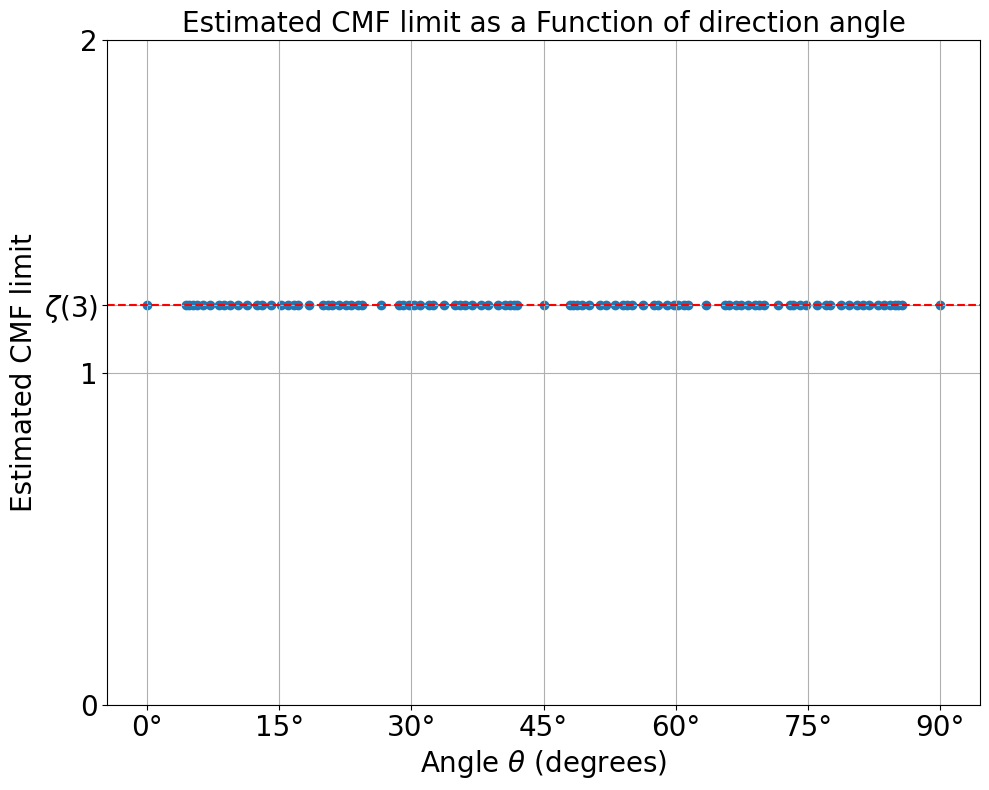
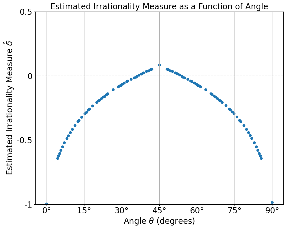
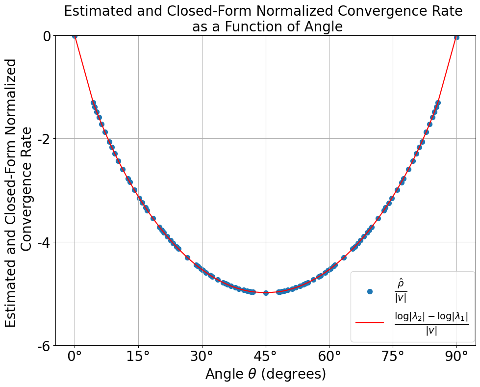
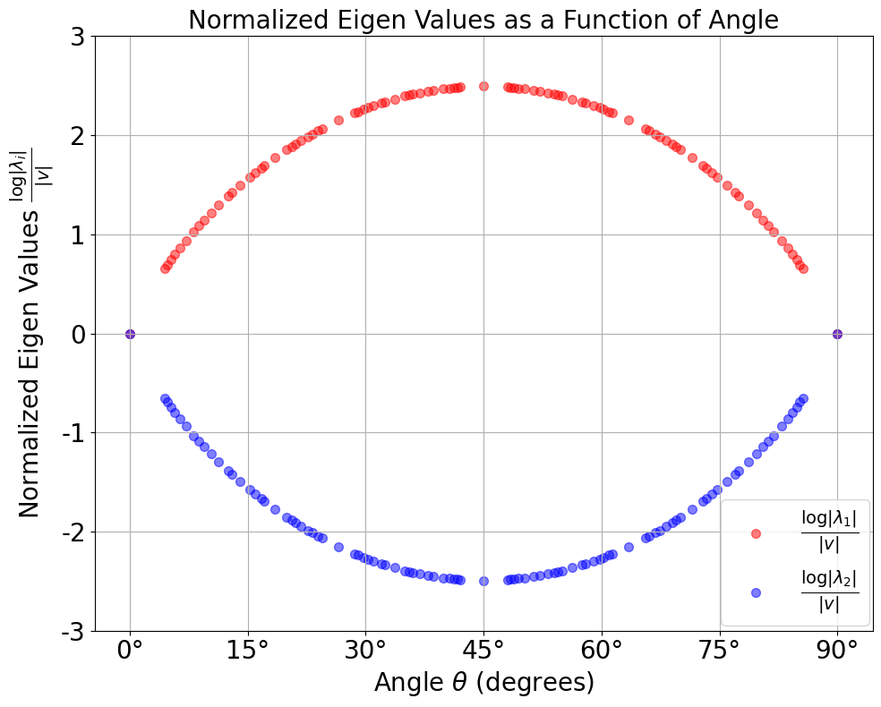
Figure 3: Asymptotic and arithmetic properties of the CMF from Example 4, VS the direction of \(v\in\mathbb{N}^2\). In all the figures above, the parameters are plotted as function of the angle of \(v\) with the \(x_1\) axis. Top Left: The estimated limit \(\hat{l} = \mathcal{L}_{x,v}^{p,q}(1000)\). In red – the value of \(\zeta(3)\). Top Right: The estimated irrationality measure \(\hat{\delta}\). in black – the cutoff for irrationality \(\delta = 0\). Note the span of directions for which \(\mathcal{L}_{x,v}^{p,q}(n)\) seems to prove the irrationality of \(\zeta(3)\). Bottom Left: The normalized convergence rate. In blue dots – the estimated value \(\frac{\hat{\rho}}{\left| v \right|}\), In red line – the closed-form value: \(\frac{\log\left| \lambda_2 \right|-\log\left| \lambda_1 \right|}{\left| v \right|}\). Bottom Right: The normalized eigenvalues \(\frac{\log\left| \lambda_i \right|}{\left| v \right|}\)..
Next, we will examine the CMF generated by the D-finite function \(\begingroup \pFqmuskip=8mu\relax \mathcode`\,=\string"8000 \begingroup\lccode`\~=`\, \lowercase{\endgroup\let~}\mskip\pFqmuskip
{}_{2}F_{1}{\left[\genfrac..{0pt}{}{2(x_1-x_2),2x_1+x_2}{x_1+2x_2};-1\right]} \endgroup\). The generators of this CMF are available in the Appendix 7. It can also be thought of as an evaluation of a sub CMF of
\(\mathcal{M}^{{}_2F_1}\) (see Appendix 6 for the definition of sub CMF). We will examine the sequences \(\mathcal{L}_{x,v}^{p,q}\) of this CMF for
\(x = (\frac{1}{3},-\frac{1}{3}), p = (1,0),q = (0,1)\), and varying on \(v\in \left\{ (a,b)\in\mathbb{Z}^2,\gcd(a,b) = 1,\left| (a,b) \right|<12 \right\}\). For each of the \(264\) trajectories, we calculated \(\hat{l},\hat{\delta},\frac{\hat{\rho}}{\left| v \right|},\frac{\log\left| \lambda_i \right|}{\left| v \right|}\) with \(N =
100\). We have plotted these quantities as function of the angle of \(v\) with the \(x_1\) axis in Figure 4.
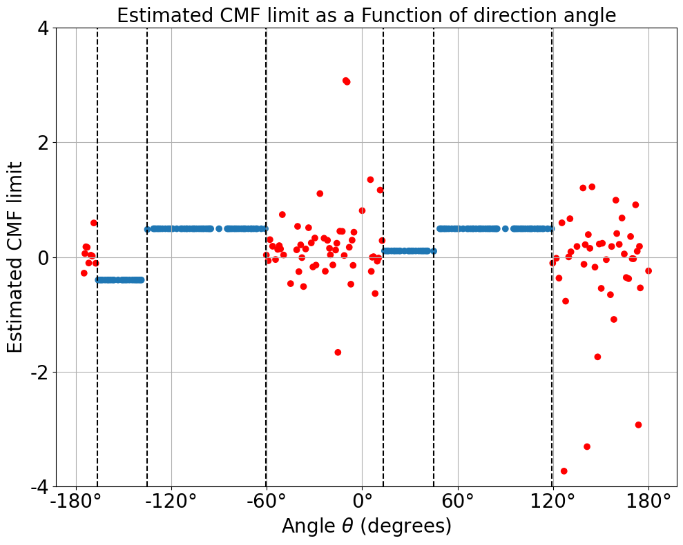
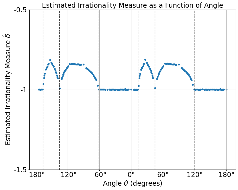
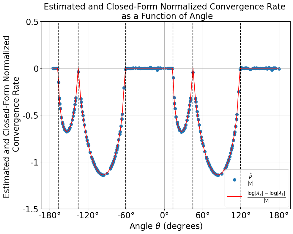
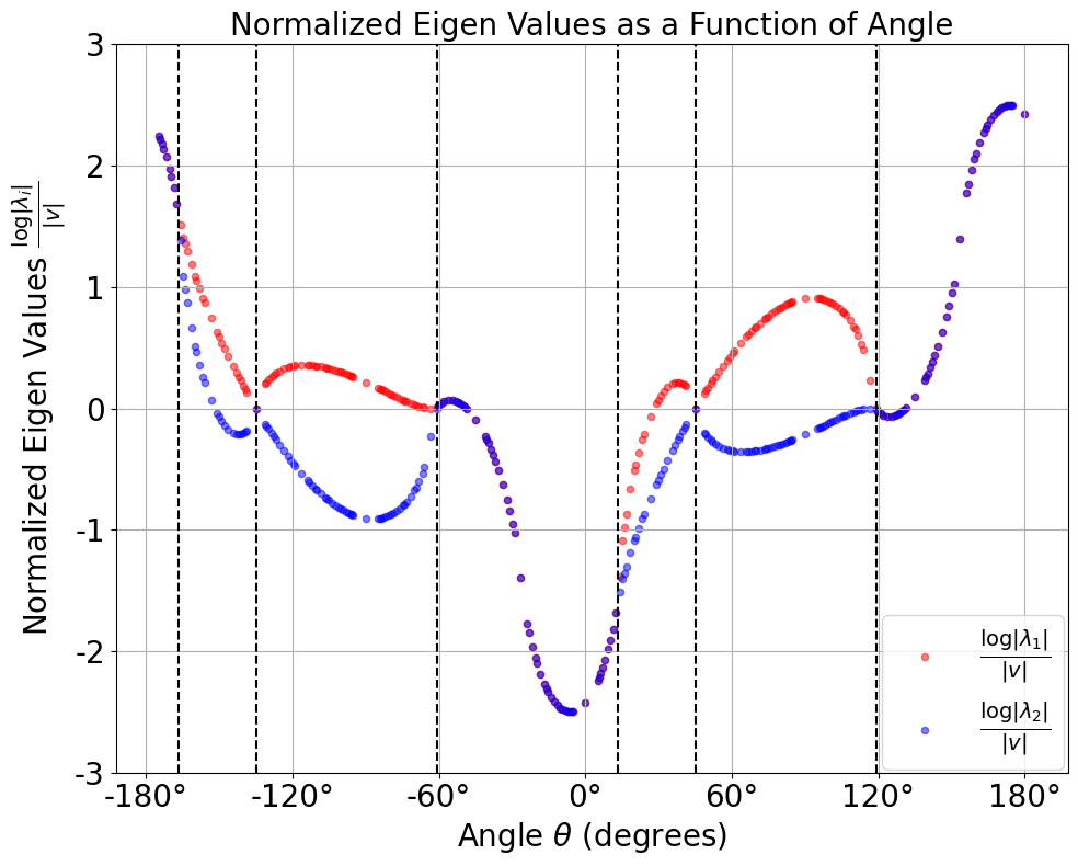
Figure 4: Asymptotic and arithmetic properties of the CMF in Appendix 7, VS the direction of \(v\in\mathbb{Z}^2\). In all the figures above, the parameters are plotted as function of the angle of \(v\) with the \(x_1\) axis, and critical angles are marked by black dashed lines. Top Left: The estimated limit \(\hat{l} = \mathcal{L}_{x,v}^{p,q}(100)\). In red – values for which the CMF ratio \(\mathcal{L}_{x,v}^{p,q}(n)\) does not converge (for an example of such a CMF ratio, see Figure 2) . Top Right: The estimated irrationality measure \(\hat{\delta}\). Bottom Left: The normalized convergence rate. In blue dots – the estimated value \(\frac{\hat{\rho}}{\left| v \right|}\), In red line – the closed-form value: \(\frac{\log\left| \lambda_2 \right|-\log\left| \lambda_1 \right|}{\left| v \right|}\). Bottom Right: The normalized eigenvalues \(\frac{\log\left| \lambda_i \right|}{\left| v \right|}\). Note: The intervals where \(\mathcal{L}_{x,v}^{p,q}(n)\) does not converge, and the points where the limits \(\hat{l}\) jump, are the points where the estimated convergence rate \(\hat{\rho}\) is \(0\), the estimated irrationality measure \(\hat{\delta}\) is \(-1\), and the eigenvalues have the same absolute value..
Finally, let us examine the CMF detailed in Example 7, generated by: \[M_{1} =\begin{pmatrix}-9 & 2 & 2\\-38 & 11 & 4\\-24 & 4 & 7\end{pmatrix}\quad M_{2} = \begin{pmatrix}\frac{119}{6} & - \frac{7}{6} & - \frac{37}{6}\\\frac{343}{6} & - \frac{11}{6} & - \frac{119}{6}\\39 & - \frac{7}{3} & -12\end{pmatrix}\] We will examine the sequences \(\mathcal{L}_{x,v}^{p_1,q_1}\) and \(\mathcal{L}_{x,v}^{p_2,q_2}\) of this CMF for \(x = (0,0,0), p_1 = (1,0,0),q_1 = (0,1,0), p_2 = (-1,-1,2),q_2 = (3,-1,0)\), and varying on \(v\in \left\{ (a,b)\in\mathbb{Z}^2,\gcd(a,b) = 1,\left| (a,b) \right|<12 \right\}\). For each of the \(264\) trajectories, we calculated \(\hat{l},\hat{\delta},\hat{\rho}\) separately for each CMF ratio, with \(N = 200\). Denoting \(\hat{l}_1,\hat{\delta}_1,\hat{\rho}_1\) for \(\mathcal{L}_{x,v}^{p_1,q_1}\), and \(\hat{l}_2,\hat{\delta}_2,\hat{\rho}_2\) for \(\mathcal{L}_{x,v}^{p_2,q_2}\). We have plotted these quantities as function of the angle of \(v\) with the \(x_1\) axis in Figure 5.


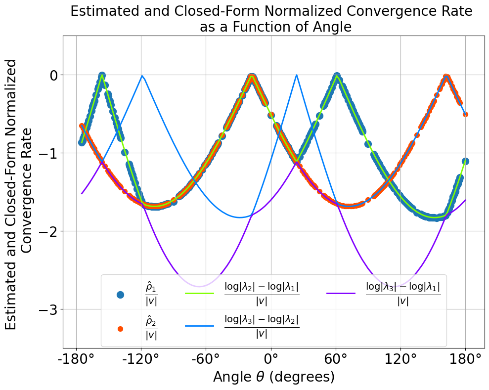
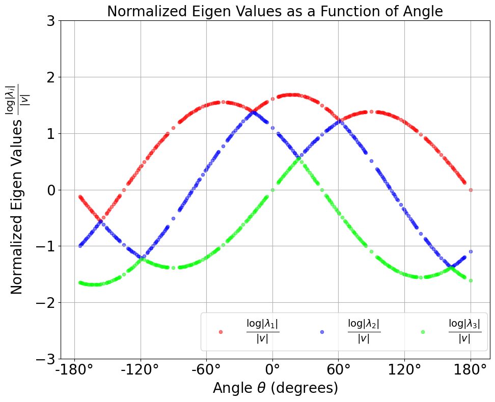
Figure 5: Asymptotic and arithmetic properties of the constant CMF in Example 7, VS the direction of \(v\in\mathbb{Z}^2\). In all the figures above, the parameters are plotted as function of the angle of \(v\) with the \(x_1\) axis, where the parameters of \(\mathcal{L}_{x,v}^{p_1,q_1}(n)\) are in blue, and the parameters of \(\mathcal{L}_{x,v}^{p_2,q_2}(n)\) are in orange. (the eigenvalues and closed-form convergence rates are independent of the choice of \(p,q\)) Top Left: The estimated limits \(\hat{l}_1,\hat{l}_2\). Top Right: The estimated irrationality measures \(\hat{\delta}_1,\hat{\delta}_2\). Bottom Left: The normalized convergence rates. In dots – the estimated values \(\frac{\hat{\rho}_i}{\left| v \right|}\), In lines – the closed-form values: \(\frac{\log\left| \lambda_j \right|-\log\left| \lambda_i \right|}{\left| v \right|}\) Note: there are 3 possible closed-form values, depending on which eigenvalues are part of the asymptotic expansion of the sequence. Bottom Right: The normalized eigenvalues \(\frac{\log\left| \lambda_i \right|}{\left| v \right|}\). Note that the set of eigenvalues \(\left\{ \log\left| \lambda_i \right|:i\in[3] \right\}\) is 3 sine waves..
5.1 Observations and Conjectures↩︎
This subsection details some observations arising from the simulations graphed in Figures 3-5. Based on these observations, we propose several conjectures to motivate future research.
Upon examining Figures 3-5, one observes that where it is defined, the CMF limit \(\lim_{n\to\infty}\mathcal{L}_{x,v}^{p,q}(n)\) appears to be constant as function of the direction of \(v\), except for finite number of discontinuities. Moreover, in domains where the convergence rate is not trivial, the limit is defined and seems constant. This observation is formalized in the following conjecture:
Conjecture 1. Let \(v_0\in\mathbb{Z}^d\setminus\left\{ 0 \right\}\), and suppose \(\mathcal{L}^{p,q}_{x,v_0}(n)\) converges to \(l\in\mathbb{R}\), with non-trivial convergence rate. Then there exists an angular domain \(D_{v_0}\in\mathbb{S}^{d-1}\) around \(\frac{v_0}{\left| v_0 \right|}\) such that for all \(v\) in that angular domain (meaning \(v\in\left\{ v\in\mathbb{Z}^d\setminus\left\{ 0 \right\}:\frac{v}{\left| v \right|}\in D_{v_0} \right\}\)) , \(\mathcal{L}^{p,q}_{x,v}(n)\to l\).
Upon examining Figures 3-5, one observes that \(\delta,\frac{\rho}{\left| v \right|},\frac{\log\left| \lambda_i \right|}{\left| v \right|}\) are all continuous with respect to the direction of \(v\) (at least where these are defined). These observations are formalized in the following conjectures:
Conjecture 2. Let \(v_0\in\mathbb{Z}^d\setminus\left\{ 0 \right\}\), and suppose \(\mathcal{L}^{p,q}_{x,v_0}(n)\) converges to \(l\in\mathbb{R}\), with non-trivial convergence rate \(\rho<0\) and irrationality measure \(\delta>-1\). Then, for any \(\varepsilon>0\), there exists an angular domain \(D_{v_0}\in\mathbb{S}^{d-1}\) around \(\frac{v_0}{\left| v_0 \right|}\) such that for all \(v\in D_{v_0}\), the irrationality measure of \(\mathcal{L}^{p,q}_{x,v}\) is in \((\delta-\varepsilon,\delta+\varepsilon)\)
Either verifying, or disproving Conjecture 2 seems challenging, due to the difficulty of establishing the irrationality measure of any particular sequence.
Conjecture 3. Let \(v_0\in\mathbb{Z}^d\setminus\left\{ 0 \right\}\), and suppose \(\mathcal{L}^{p,q}_{x,v_0}(n)\) converges to \(l\in\mathbb{R}\), with non-trivial convergence rate \(\rho<0\). Then, for any \(\varepsilon>0\), there exists an angular domain \(D_{v_0}\in\mathbb{S}^{d-1}\) around \(\frac{v_0}{\left| v_0 \right|}\) such that for all \(v\in D_{v_0}\), the normalized convergence rate of \(\mathcal{L}^{p,q}_{x,v}\) is in \((\frac{\rho}{\left| v_0 \right|}-\varepsilon,\frac{\rho}{\left| v_0 \right|}+\varepsilon)\)
Conjecture 4. Let \(v_0\in\mathbb{Z}^d\setminus\left\{ 0 \right\}\), and suppose \(T_{x,v_0}(n)\) is coboundary equivalent to a companion matrix whose recurrence \(L\) satisfies the Poincaré Perron conditions, with eigenvalues \((\lambda_1,\dots,\lambda_r)\). Then, for any \(\varepsilon>0\), there exists an angular domain \(D_{v_0}\in\mathbb{S}^{d-1}\) around \(\frac{v_0}{\left| v_0 \right|}\) such that for all \(v\in D_{v_0}\), \(T_{x,v}(n)\) is coboundary equivalent to a companion matrix who satisfies the Poincaré Perron conditions, and the \(i\)-th normalized eigenvalue of \(T_{x,v}(n)\) is in \((\frac{\log\left| \lambda_i \right|}{\left| v_0 \right|}-\varepsilon,\frac{\log\left| \lambda_i \right|}{\left| v_0 \right|}+\varepsilon)\)
Remark 14. Notice that as detailed in Remark 8, the height of a sequence can be directly ascertained from its convergence rate and irrationality measure (if both are non trivial). Specifically: \[\eta = -\frac{\rho}{\delta+1}\] Thus, if Conjectures 2,3 hold, we have that the normalized height \(\frac{\eta}{\left| v \right|}\) is also continuous. Furthermore, if any two of \(\delta, \frac{\rho}{\left| v \right|},\frac{\eta}{\left| v \right|}\) are continuous in the direction of \(v\), then they all are.
It is straight forward to prove Conjectures 1,3 and 4 for the constant CMF described in Example 7. This, by noting that as \(M_{x_1},M_{x_2}\) commute, they share eigen spaces. And as they are both diagonalizeable, they are simultaneously diagonalizeable. As similarity over \(\text{GL}_r(\mathbb{C})\) is a special case of coboundary equivalence, our CMF is coboundary equivalent to one generated by: \[\overline{M}_{x_1} = \begin{pmatrix} 5&0&0\\ 0&3&0\\ 0&0&1 \end{pmatrix},\overline{M}_{x_2} = \begin{pmatrix} \frac{5}{3}&0&0\\ 0&\frac{1}{3}&0\\ 0&0&4 \end{pmatrix}\] and using Proposition 10, the rest falls out naturally. The differences in \(\rho,\delta\) between the two ratios \(\mathcal{L}_{x,v}^{p_1,q_1}(n),\mathcal{L}_{x,v}^{p_2,q_2}(n)\) can be explained by \(p_2,q_2\) being spanned by only two of the eigen vectors of \(M_{x_1},M_{x_2}\). It is not hard to generalize these arguments and justify Conjectures 1,3, and 4 for any conservative matrix field with constant matrices.
5.2 Applications and Corollaries↩︎
Conjectures 1,2, if true, imply interesting properties, and motivate algorithms for the search and analysis of good approximations for constants.
Corollary 5. Assuming Conjectures 1,2 hold for a
CMF \(\mathcal{M}\) of dimension \(d\) and rank \(r\), and suppose further \(\mathcal{L}_{x,v_0}^{p,q}(n)\) converges to
\(l\in\mathbb{R}\) with irrationality measure \(\delta>0\). Then there exists an angular domain \(D_{v_0}\in\mathbb{S}^{d-1}\) around \(\frac{v_0}{\left| v_0 \right|}\) such that for all \(v\) in that angular domain (meaning \(v\in\left\{ v\in\mathbb{Z}^d\setminus\left\{ 0 \right\}:\frac{v}{\left| v
\right|}\in D_{v_0} \right\}\)) , \(\mathcal{L}^{p,q}_{x,v_0}(n)\to l\) with positive irrationality measure.
Put simply - one irrationality proving sequence in a CMF, implies infinitely many (essentially different) irrationality proving sequences.
Remark 15. Assuming Conjectures 1,2 hold for a CMF \(\mathcal{M}\) of dimension \(d\) and rank \(r\), and suppose that \(\mathcal{L}_{x,v_0}^{p,q}(n)\) converges to \(l\in\mathbb{R}\) with irrationality measure \(\delta>-1\). Then, it is possible to use an optimization algorithm to search for \(v\) such that \(\mathcal{L}_{x,v}^{p,q}(n)\) converges to \(l\) with higher irrationality measure.
Let us expand on Remark 15. Often, when D-finite ratios appear in the literature, they are generated as a sequence of values from some D-finite function,
usually of several variables. like hypergeometric functions, integrals in several variables, binomial sums, etc. Thus, one can examine record results for \(\zeta(5),\pi,G,\dots\), generate a CMF from the multivariate
D-finite function used in their construction, and associate the D-finite ratio with a CMF ratio \(\mathcal{L}_{x,v}^{p,q}(n)\). Then, the usage of optimization algorithms as described in Remark 15 might result in an improvement to the record result.
This, we hope, should not only generate interest in CMF ratios, but also in proving the suggested conjectures.
Acknowledgments↩︎
This research received support through Schmidt Sciences, LLC.
The authors also wish to acknowledge the use of the HolonomicFunctions package developed by Christoph Koutschan [33] and the Asymptotics package by Manuel Kauers [34]. The first author is grateful to Frédéric Chyzak and Tali Monderer for their insightful discussions.
6 Dual CMF, and Sub CMF↩︎
Definition 18. Let \(\mathcal{M}\) be a CMF of dimension \(d\) rank \(r\) over \(K\). Then, the Dual CMF* of \(\mathcal{M}\), \(\mathcal{M}^*\) is a CMF of dimension \(d\) rank \(r\) over \(K\) satisfying: \[\forall_{v\in\mathbb{Z}^d}\;\mathcal{M}^*_v = (\mathcal{M}_v^{-1})^t\]*
Definition 19. Let \(\mathcal{M}\) be a CMF of dimension \(d\) rank \(r\) over \(K\). Let \(\Lambda\) be a sub lattice of \(\mathbb{Z}^d\), and let \((l_1,\dots,l_s)\) be a basis of \(\Lambda\), and \((l_1,\dots,l_s,l_{s+1},\dots,l_{d})\) be a basis of \(\mathbb{Z}^d\).
Then, the matrices \(\mathcal{M}_{l_1},\dots,\mathcal{M}_{l_s}\) can be rewritten as members of \(\text{GL}_r(K(l_1,\dots,l_d))\), and in that form they generate a CMF of dimension \(s\) rank \(r\) over \(K(l_{s+1},\dots,l_d)\). Such a CMF is called a Sub-CMF* of \(\mathcal{M}\).*
Remark 16. Trajectory matrices \(T_{x,v}(n)\) are evaluations of the sub-CMF associated with \(\Lambda = \left\{ kv:k\in\mathbb{Z} \right\}\)
7 CMF generated by \(\begingroup \pFqmuskip=8mu\relax \mathcode`\,=\string"8000 \begingroup\lccode`\~=`\, \lowercase{\endgroup\let~}\mskip\pFqmuskip {}_{2}F_{1}{\left[\genfrac..{0pt}{}{2(x_1-x_2),2x_1+x_2}{x_1+2x_2};-1\right]} \endgroup\)↩︎
The CMF analyzed in Figure 4 is a CMF of dimension \(2\) and rank \(2\), generated by the following matrices: \[M_1 = \begin{pmatrix} \frac{\left(x_{1} + 2 x_{2}\right) \left(3 x_{1} - 3 x_{2} + 2\right)}{\left(2 x_{1} + x_{2} + 1\right) \left(8 x_{1} - 8 x_{2} + 4\right)} & - \frac{\left(x_{1} + 2 x_{2}\right) \left(7 x_{1}^{2} + x_{1} \left(11 - 8 x_{2}\right) + x_{2}^{2} - 5 x_{2} + 4\right)}{\left(2 x_{1} + x_{2} + 1\right) \left(16 x_{1} - 16 x_{2} + 8\right)}\\\frac{\left(x_{1} + 2 x_{2}\right) \left(7 x_{1}^{2} - 8 x_{1} x_{2} + 5 x_{1} + x_{2}^{2} + x_{2}\right)}{\left(x_{1} - x_{2}\right) \left(2 x_{1} + x_{2}\right) \left(2 x_{1} + x_{2} + 1\right) \left(16 x_{1} - 16 x_{2} + 8\right)} & - \frac{\left(x_{1} + 2 x_{2}\right) \left(11 x_{1}^{3} + x_{1}^{2} \left(3 x_{2} + 14\right) + x_{1} \left(- 3 x_{2}^{2} + 20 x_{2} + 1\right) - 11 x_{2}^{3} + 2 x_{2}^{2} + 11 x_{2} - 2\right)}{\left(x_{1} - x_{2}\right) \left(2 x_{1} + x_{2}\right) \left(2 x_{1} + x_{2} + 1\right) \left(32 x_{1} - 32 x_{2} + 16\right)} \end{pmatrix}\] \[M_2 = \begin{pmatrix} P_{1,1} & P_{1,2}\\ P_{2,1} & P_{2,2} \end{pmatrix}\] Where: \[P_{1,1} = \frac{\left(x_{1} + 2 x_{2}\right) \left(x_{1} + 2 x_{2} + 1\right) \left(7 x_{1}^{2} - x_{1} \left(50 x_{2} + 19\right) + 79 x_{2}^{2} + 67 x_{2} + 10\right)}{\left(x_{1} - 4 x_{2}\right) \left(x_{1} - 4 x_{2} - 1\right) \left(x_{1}^{2} - x_{1} \left(8 x_{2} + 5\right) + 16 x_{2}^{2} + 20 x_{2} + 6\right)}\] \[P_{1,2} = - \frac{\left(2 x_{1} + 4 x_{2}\right) \left(x_{1} + 2 x_{2} + 1\right) \left(6 x_{1}^{3} - 3 x_{1}^{2} \left(15 x_{2} + 7\right) + x_{1} \left(90 x_{2}^{2} + 96 x_{2} + 22\right) - 51 x_{2}^{3} - 93 x_{2}^{2} - 49 x_{2} - 7\right)}{\left(x_{1} - 4 x_{2}\right) \left(x_{1} - 4 x_{2} - 1\right) \left(x_{1}^{2} - x_{1} \left(8 x_{2} + 5\right) + 16 x_{2}^{2} + 20 x_{2} + 6\right)}\] \[P_{2,1} = \frac{\left(6 x_{1} + 12 x_{2}\right) \left(x_{1} + 2 x_{2} + 1\right) \left(2 x_{1}^{3} - 3 x_{1}^{2} \left(5 x_{2} + 2\right) + x_{1} \left(30 x_{2}^{2} + 27 x_{2} + 4\right) - x_{2} \left(17 x_{2}^{2} + 21 x_{2} + 6\right)\right)}{\left(x_{1} - 4 x_{2}\right) \left(x_{1} - x_{2}\right) \left(2 x_{1} + x_{2}\right) \left(x_{1} - 4 x_{2} - 1\right) \left(x_{1}^{2} - x_{1} \left(8 x_{2} + 5\right) + 16 x_{2}^{2} + 20 x_{2} + 6\right)}\] \[P_{2,2} = - \frac{4 \left(x_{1} + 2 x_{2}\right) \left(- x_{1} + x_{2} + 1\right)^{2} \left(x_{1} + 2 x_{2} + 1\right) \left(4 x_{1}^{2} - 2 x_{1} \left(10 x_{2} + 3\right) + x_{2} \left(7 x_{2} + 3\right)\right)}{\left(x_{1} - 4 x_{2}\right) \left(x_{1} - x_{2}\right) \left(2 x_{1} + x_{2}\right) \left(x_{1} - 4 x_{2} - 1\right) \left(x_{1}^{2} - x_{1} \left(8 x_{2} + 5\right) + 16 x_{2}^{2} + 20 x_{2} + 6\right)}\]
References↩︎
Corresponding author: shacharwein@gmail.com↩︎
Corresponding author: kaminer@technion.ac.il↩︎
Our formulation is not as general as the original, as we are interested only in D-finite sequences.↩︎
As a matter of fact, a conservative matrix field is an Eilenberg–MacLane 1-cocycle of \(\mathbb{Z}^d\) with non-abelian coefficients \(\text{GL}_r(K(\mathbf{x}))\).↩︎