1 Introduction↩︎

The simulation of transport phenomena involving chemically reactive species plays a key role in many environmental and engineering applications, such as groundwater contamination, and the modeling of water and air quality. These processes are governed by advection–diffusion–reaction systems, where the advective term is associated with a flow model satisfying a continuity equation, i.e., the conservation of mass.

A wide variety of numerical methods have been proposed to solve these kinds of problems; see, e.g., [1], [2] and [3] for a comprehensive review. In general, these approaches can be divided into two main families. The first ones are the Streamline Diffusion (SD) methods, which rely on a continuous Galerkin formulation [4]. The second ones include Discontinuous Galerkin (DG) methods [5], [6].

When the exact velocity field is used, both SD and DG methods are known to be stable, accurate, and globally conservative. However, when an approximate velocity field is employed, these schemes may lose two essential properties: zeroth-order accuracy and/or global conservation.

The first property refers to the ability to preserve constant solutions. In an advection–diffusion–reaction problem with constant initial, boundary, and source data, the exact solution remains constant in time. A method which is zeroth-order accurate is able to numerically reproduce this behavior. If it is not, spurious sources or sinks may appear. The second property, global conservation, ensures that the total mass varies only due to fluxes across the domain boundary.

Interestingly, SD and DG schemes exhibit complementary behavior in this regard. SD schemes preserve zeroth-order accuracy, but ensure global conservation only under restrictive conditions on the velocity field [3]. Conversely, DG schemes guarantee global conservation regardless of the velocity approximation, but may fail to preserve constant solutions unless additional compatibility conditions are imposed.

In this work, we consider the coupling between an advection—diffusion–reaction system and a velocity field obtained from a Darcy problem. The Darcy equation is discretized by the Mixed Virtual Element Method [7], [8], while the time–dependent advection–diffusion–reaction equation is solved using the Virtual Element Method (VEM) for spatial discretization [7], [9] combined with a Discontinuous Galerkin time-stepping scheme [10], following the approach proposed in [11]. For the time discretization, we adopt a Gauss–Radau quadrature formula with respect to the temporal variable [10]. This choice leads to high–order, fully discrete time–integration schemes well suited for adaptive temporal refinement. As a consequence, while the proposed continuous VEM formulation is exact for zeroth-order polynomial solutions, unlike DG schemes it does not inherently guarantee the global mass conservation of the scalar concentrations. The main contributions of this paper are:

• the proof of existence and uniqueness of the proposed semi-discrete and fully discrete VE–DG schemes within this kind of problem;

• the derivation of error estimates in suitable discrete norms;

• the extension of the analysis to the case of multiple species coupled through a first-order reaction network.

The remainder of the paper is organized as follows. In Section 2, we introduce the governing equations for both the Darcy and the transport problems, along with the underlying model assumptions and the well-posedness of the continuous formulation. In Section 3, we briefly describe the Virtual Element spaces employed for the discretization, focusing on the projection operators and the properties essential for the subsequent analysis. Section 4 represents the core of the work; here, we define the semi-discrete and fully discrete formulations, establishing their well-posedness and deriving the corresponding error estimates. Finally, in Section 5, we present several numerical experiments to validate the proposed approach, including one applicative test case involving the interaction of two species.

1.0.0.1 Notation.

Throughout this article we adopt the standard notation for function spaces and operators [12]–[16]. Specifically, we denote by \(\partial_t\) the derivative with respect to time, and by \(\nabla\) and \(\Delta\) the spatial gradient and Laplace operator, respectively. Given an open and bounded domain \(\mathcal{D} \subset \mathbb{R}^2\), \(p\in [1,\infty]\) and \(s\ge 0\), we denote by \(L^p(\mathcal{D})\) the standard Lebesgue space with norm \[\|u\|_{0,p,\mathcal{D}} = \begin{cases} \left( \displaystyle\int_{\mathcal{D}} |u(\boldsymbol{x})|^p\,d\boldsymbol{x}\right)^{1/p}, & 1 \le p < \infty, \\[0.6em] \operatorname*{ess\,sup}_{\boldsymbol{x}\in \mathcal{D}} |u(\boldsymbol{x})|, & p = \infty, \end{cases}\] and by \(W^{m,p}(\mathcal{D})\) the standard Sobolev space \[W^{m,p}(\mathcal{D}) = \{ u \in L^p(\mathcal{D}) : D^\alpha u \in L^p(\mathcal{D}),\;\text{ for all }|\alpha| \le m \},\] endowed with the usual seminorm and norm, denoted by \(|\cdot|_{m,p,\mathcal{D}}\) and \(\|\cdot\|_{m,p,\mathcal{D}}\), respectively. The space \(L^2(\mathcal{D})\) is a Hilbert space endowed with the usual inner product \((u,v)_{\mathcal{D}}\). When \(p=2\), we use the shorter notation \(H^s(\mathcal{D}):=W^{s, 2}(\mathcal{D})\). As before, its seminorm and norm are denoted by \(|\cdot|_{s,\mathcal{D}}\) and \(\|\cdot\|_{s,\mathcal{D}}\), respectively. Let \(H_0^1(\mathcal{D})\) denote the subspace of \(H^1(\mathcal{D})\) consisting of functions with zero trace on \(\partial\mathcal{D}\). We denote by \(W^{-m,\frac{p}{p-1}}(\mathcal{D})\) the dual of the space \(W^{m,p}(\mathcal{D})\) with the usual convention \(H^{-m}(\mathcal{D})\) for the case \(p=2\).

Furthermore, given \(p\in [1,\infty]\),  \(s \geq 1\), a Banach space \((X, \|\cdot\|_X)\), and a time interval \((a,b)\), the corresponding Lebesgue-Bochner space is defined by \[L^p(a,b;X) = \{ u : (a,b) \to X \text{ strongly measurable},\;\|u\|_{L^p(a,b;X)} < \infty \},\] with \[\|u\|_{L^p(a,b;X)} = \begin{cases} \left( \displaystyle\int_a^b \|u(t)\|_X^p\,dt \right)^{1/p}, & 1 \le p < \infty, \\[0.6em] \operatorname*{ess\,sup}_{t \in (a,b)} \|u(t)\|_X, & p = \infty, \end{cases}\] and by \[W^{s,p}(a,b;X) = \{ u \in L^p(a,b;X) : \partial_t^j u \in L^p(a,b;X),\text{ for all }1 \le j \le s \},\] equipped with the norm \[\|u\|_{W^{s,p}(a,b;X)} = \left( \sum_{j=0}^{k} \| \partial_t^j u \|_{L^p(a,b;X)}^p \right)^{1/p}.\] When \(p=2\), we use the Hilbertian notation \(H^s(a,b;X) := W^{s,2}(a,b;X)\).

To facilitate the reader’s navigation through the complex structure of the problem, we adopt a consistent typographical convention for the different types of variables involved. Throughout this work, standard italic letters (e.g., \(u, w\)) denote scalar-valued functions defined in \(\mathbb{R}\). Boldface letters (e.g., \(\mathbf{u}, \mathbf{n}\)) are reserved for vector fields in the physical space \(\mathbb{R}^d\). Finally, to distinguish the multi–component nature of certain variables, specifically the presence of \(n_c\) species, Fraktur symbols (e.g., \(\mathfrak{v}, \mathfrak{w}\)) are employed for vectors belonging to the generalized space \(\mathbb{R}^{n_c}\). This distinction is systematically maintained to ensure clarity across the different mathematical dimensions of the model.

Regarding functional spaces, we extend the previously defined notations to the multi–component framework. For instance, the space of functions whose components are in \(H^1(\Omega)\) for each of the \(n_c\) components is denoted by \([H^1(\Omega)]^{n_c}\). Similarly, an element \(\mathfrak{v} \in [H^1(\Omega)]^{n_c}\) represents the vector \((v_1, \dots, v_{n_c})\), where each \(v_i \in H^1(\Omega)\).

Finally, we use the notation \(a\lesssim b\) to indicate the existence of a positive constant \(C\), independent of the mesh size, the element diameters, and the edge lengths, such that \(a \leq C\,b\). Furthermore, we use the notation \(a\approx b\) to indicate that \(a\lesssim b\) and \(b\lesssim a\).

2 Model problem↩︎

In this section, we describe the multi-species model problem considered in this article. In Sections 2.1 and 2.2, we introduce the strong formulations of the Darcy and transport equations, respectively. Then, in Section 2.3, we analyze in more detail how these two equations are coupled in this class of problems and describe the simplifications adopted in this work. Based on these assumptions, we define the weak formulation of the problem in Section 2.4. Finally, Section 2.5 is devoted to establishing the theoretical framework and to proving the existence and uniqueness of the solution.

2.1 Darcy equations↩︎

We consider the classical Darcy equation in mixed form that describes the flow of a fluid through a porous medium. In this model, the velocity field, \(\boldsymbol{u}:\Omega \rightarrow \mathbb{R}^2\), satisfies the conservation of mass equation of the form \[\label{continuityeq} \text{div}(\boldsymbol{u}) =f,\tag{1}\] where \(\boldsymbol{u}\) is the velocity field, and \(f\) is an external source or sink term. Specifically, sources are characterized by positive values of \(f\), while sinks correspond to negative ones.

Darcy’s law for the flow of a viscous fluid in a permeable medium is expressed as follows: \[\label{darcyslaw} \boldsymbol{u}=\dfrac{K}{\mu (c_1,...,c_{n_c})}\nabla p, \text{ in }\Omega,\tag{2}\] where \(p:\Omega \rightarrow \mathbb{R}\) denotes the pressure, \(K\) is the permeability coefficient, and \(\mu\) is the viscosity of the fluid which generally depends on the species concentrations. The boundary of \(\Omega\), denoted by \(\Gamma\), is partitioned into two parts \(\overline{\Gamma_N}\cup\overline{\Gamma_D}\) with \(\Gamma_N\cap \Gamma_D=\emptyset\). We impose the following boundary conditions: \[\begin{align} \tag{3} p&=g_D, \quad\text{on }\Gamma_D,\\ \tag{4} \boldsymbol{u}\cdot \boldsymbol{n}&=g_N, \quad \text{on } \Gamma_N, \end{align}\] here \(\boldsymbol{n}\) denotes the outward pointing unit normal to \(\Gamma\), \(g_D\in \mathrm{H}_{00}^{1/2}(\Gamma_D)\) and \(g_N\in \mathrm{H}_{00}^{-1/2}(\Gamma_N)\) are the Dirichlet and Neumann boundary data, respectively.

2.2 Transport equations↩︎

Given a set of \(n_c\) species, whose initial distribution in the domain \(\Omega\) is a known function \(c_i^0\) for \(i=1,\dots,n_c\), we consider the following transport equations for each species \[\partial_t {c}_i+\text{div}(\boldsymbol{u}\,{c_i}-D_i(\boldsymbol{u})\nabla c_i)=f c_i^{\ast}+R_i(c_1,\dots,c_{n_c})\quad\text{for }i=1,\dots,n_c. \label{Mtransport}\tag{5}\] Here \(c_i\) denotes the concentration of the \(i\)-th species, and the symmetric positive semi-definite tensor \(D_i(\boldsymbol{u})\) represents the diffusion-dispersion of the \(i\)-th species which, in general, depends on the Darcy flow \(\boldsymbol{u}\). The function \(c_i^\ast\) represents the prescribed concentration of the \(i\)-th species at sources or sinks. Specifically, it is defined according to the sign of the Darcy force term \(f\): for sources \(f>0\), \(c_i^\ast\) is a given function \(\tilde{c}_i\), whereas for sinks \(f<0\) it coincides with the concentration, i.e., \(c_i^\ast=c_i\). Finally, \(R_i\) is the reaction term which may depend on all species, including the \(i\)-th one.

The boundary \(\Gamma\) for the transport system is split into two disjoint parts: \[\label{binoutflow} \Gamma_{I}:=\{ \boldsymbol{x}\in \Gamma:\, \boldsymbol{u}\cdot\boldsymbol{n}<0\}\quad\text{and}\quad\Gamma_{O}:=\{ \boldsymbol{x}\in \Gamma:\, \boldsymbol{u}\cdot\boldsymbol{n}\geq 0\},\tag{6}\] representing the inflow and the outflow boundary, respectively. On these boundaries, we impose the following boundary conditions \[\begin{equation}\tag{7} (c_i\boldsymbol{u}-D_i(\boldsymbol{u})\nabla c_i)\cdot \boldsymbol{n}=c_i^I\boldsymbol{u}\cdot \boldsymbol{n}, \qquad \text{on }\Gamma_{I}\times (0,T], \end{equation} \begin{equation}\tag{8} \qquad \qquad D_i(\boldsymbol{u})\,\nabla c_i \cdot \boldsymbol{n}=0, \, \qquad \qquad \text{on }\Gamma_{O}\times (0,T]. \end{equation}\] Here \(c_i^I\) is the inflow concentration of the \(i\)-th species which may depend on both space and time.

2.3 Simplified model and assumptions↩︎

This class of problems presents several challenges due to the nonlinear relations, the time dependency and strong coupling of these two problems. Given an initial distribution of species concentrations, since the porosity \(\mu\) generally depends on the species distributions, one can compute the Darcy flow at the initial time. Then, using this velocity field \(\boldsymbol{u}\), the new concentration distribution can be obtained by solving the nonlinear time-dependent problem 5 . However, since the species concentrations evolve in time, the Darcy problem must be solved again to update the velocity field, and then the transport problem must be resolved accordingly. In summary, to obtain the concentration distribution over time, one must repeatedly alternate between solving the Darcy problem and the nonlinear time-dependent transport problem until the end of the simulation.

Dealing with such system, with all these difficulties, is extremely demanding both from a theoretical and the practical viewpoint. For this reason, in this preliminary work we introduce a series of simplifications in order to establish a foundation for future studies, where some of these complexities will be progressively reintroduced.

Specifically, the model is analyzed under the assumptions of a multi-species transport system with a first-order reaction network, the particularities of which, relative to the general model, are grounded in references [17]–[21]. In accordance with the cited literature, the assumptions governing the proposed model are as follows:

(i) more than one species may be present, i.e., \(n_c>1\);

(ii) the coefficient \(\mu\) of the Darcy flow is constant throughout the domain \(\Omega\) and is not species dependent;

(iii) the diffusion tensors \(D_i(\boldsymbol{u})\) are constant and isotropic, i.e., they can be reduced to scalar coefficients \(D_i\);

(iv) the transport of the \(n_c\) species undergoes a first-order reaction network with liquid-phase degradation; in other words, the reaction terms take the form \[R_i(c_1,\dots,c_{n_c}) = -\gamma_i c_i + \sum_{\substack{j=1\\ j\neq i}}^{n_c} y_{i/j}\,\gamma_j\,c_j, \label{reactionterm}\tag{9}\] where \(\gamma_j\) denotes the first-order degradation (or decay) rate constant of the \(j\)-th species, and \(y_{i/j}\) is the effective yield coefficient representing the mass of \(i\)-th species produced from the degradation of \(j\)-th species.

2.4 Weak formulations↩︎

In this section, we introduce the weak formulations of both the Darcy and the transport equations (see Sections 3.2 and 2.2). Let us consider the Darcy problem. First, we define the following functional spaces \[\begin{align} \mathbf{H}(\text{div},\Omega)&:=&\left\{\boldsymbol{v}\in [L^2(\Omega)]^2:\, \text{div}\,\boldsymbol{v}\in L^2(\Omega)\right\},\\[0.3em] \mathbf{H}_{N,g_N}(\text{div},\Omega)&:=&\left\{\boldsymbol{v}\in \mathbf{H}(\text{div},\Omega):\, \boldsymbol{v}\cdot \boldsymbol{n}=g_N \, \text{on} \, \Gamma_N \right\}, \end{align}\] and \[\mathbf{H}_{N,0}(\text{div},\Omega):=\left\{\boldsymbol{v}\in \mathbf{H}(\text{div},\Omega):\, \boldsymbol{v}\cdot \boldsymbol{n}=0 \, \text{on} \, \Gamma_D \right\}.\] We equip these spaces with the usual norm defined as \[\Vert \boldsymbol{v}\Vert_{\mathop{\mathrm{div}}\nolimits}^2:=\Vert \boldsymbol{v}\Vert_{0,\Omega}^2+\Vert \text{div}\, \boldsymbol{v}\Vert_{0,\Omega}^2.\] Starting from these functional spaces, to get the variational formulation of the Darcy problem, we proceed as usual. We multiply equations 1 and 2 by suitable test functions. Then, integrating by parts over \(\Omega\), we get the variational form of Darcy’s problem: find \((\boldsymbol{u},p)\in \mathbf{H}_{N,g_N}(\text{div},\Omega)\times \mathrm{L}^2(\Omega)\), such that \[\begin{align} \mathcal{M}(\boldsymbol{u},\boldsymbol{v})+ \mathcal{N}(\boldsymbol{v},p)&=\mathcal{G}_N(\boldsymbol{v}), &\forall\boldsymbol{v}\in \mathbf{H}_{N,0}(\text{div},\Omega), \tag{10}\\ \mathcal{N}(\boldsymbol{u},q)&=\mathcal{G}_D(q), &\forall q\in \mathrm{L}^2(\Omega),\tag{11} \end{align}\] where we have defined the following bilinear and linear forms \[\begin{align} \mathcal{M}(\boldsymbol{u},\boldsymbol{v})&:=\mu K^{-1}\int_{\Omega} \boldsymbol{u}\cdot \boldsymbol{v}\, d\boldsymbol{x}, \\ \mathcal{N}(\boldsymbol{v},q)&:=\int_{\Omega}q\,\text{div}\boldsymbol{v}\, d\boldsymbol{x},\\ \mathcal{G}_N(\boldsymbol{v})&:=\int_{\Gamma_N}g_N(\boldsymbol{v}\cdot \boldsymbol{n})\, dS\\ \mathcal{G}_D(q)&:=\int_{\Omega} f\,q\, d\boldsymbol{x}. \end{align}\]

We move now to the transport equations. In this case, we adopt as the functional space for the solution the Hilbert space \(\mathrm{H}^1(0, T;\mathrm{H}^1(\,\Omega))\). We now turn our attention to the transport equations. For simplicity, let us focus on the \(i\)-th species. Multiplying 5 by a test function \(w_i\in \mathrm{H}^1(\Omega)\) and integrating by parts over \(\Omega\), we obtain

\[\label{eq1} \int_{\Omega} \partial_t \,c_i\, w_i \,d\boldsymbol{x}-\int_{\Omega}(\boldsymbol{u}c_i-D_i\nabla c_i )\cdot \nabla w_i \, d\boldsymbol{x}+\int_{\Gamma}(\boldsymbol{u}c_i-D_i\nabla c_i )\cdot\boldsymbol{n}\, w_i\, dS =\int_{\Omega}(f c_i^{\ast}+R_i(\mathfrak{c}))w_i\,d\boldsymbol{x}\tag{12}\]

Here, we introduce the vector \(\mathfrak{c}\) which collects all the species so that we have a more compact notation of the reaction term \(R_i(\mathfrak{c})\) instead of \(R_i(c_1,\dots,c_{n_c})\).

Starting from this variational formulation, we manipulate these integrals in such a way that both boundary conditions and the source term of the Darcy problem appear. To do this, let \(\xi,\eta\in \mathrm{H}^1(\Omega)\) and \(\boldsymbol{g}\in \mathbf{H}(\text{div},\Omega)\cap \mathrm{\boldsymbol{L}}^4(\Omega)\cap \gamma_{\boldsymbol{n}}^{-1}(\mathrm{L}^2(\Gamma))\), exploiting by parts integration, the following identity holds \[\int_{\Omega}\text{div}(\xi\,\boldsymbol{g})\,\eta\,d\boldsymbol{x}=-\int_{\Omega}\xi\,(\boldsymbol{g}\cdot \nabla \eta)\,d\boldsymbol{x}+\int_{\Gamma}\xi\,\eta \,(\boldsymbol{g}\cdot \boldsymbol{n})\, dS\,. \label{eqn:byPart1}\tag{13}\] Then, if we compute the divergence of the left-hand side, Equation 13 becomes \[\int_{\Omega}(\xi\, \text{div}\,\boldsymbol{g}+\boldsymbol{g}\cdot \nabla \xi)\,\eta\,d\boldsymbol{x}=-\int_{\Omega}\xi\,(\boldsymbol{g}\cdot \nabla \eta)\,d\boldsymbol{x}+\int_{\Gamma}\xi\,\eta \,(\boldsymbol{g}\cdot \boldsymbol{n})\, dS,\] that gives the following identity; \[\int_{\Omega}(\boldsymbol{g}\cdot \nabla \xi)\,\eta\,d\boldsymbol{x}=\int_{\Omega}\xi\,\eta\, \text{div}\,\boldsymbol{g}\,\, d\boldsymbol{x}-\int_{\Omega}\xi\,(\boldsymbol{g}\cdot \nabla \eta)\,d\boldsymbol{x}+\int_{\Gamma}\xi\,\eta \,(\boldsymbol{g}\cdot \boldsymbol{n})\, dS.\] Assuming that \(\boldsymbol{u}\) has sufficient regularity, and setting \(\boldsymbol{g}=\boldsymbol{u}\), \(\eta=c_i\) and \(\xi=w_i\) in the previous identity, we obtain \[\begin{align} \nonumber \int_{\Omega}c_i\,(\boldsymbol{u}\cdot \nabla w_i)\,d\boldsymbol{x}&=\frac{1}{2}\left( \int_{\Omega}c_i\,(\boldsymbol{u}\cdot \nabla w_i)\,d\boldsymbol{x}+\int_{\Omega}c_i\,(\boldsymbol{u}\cdot \nabla w_i)\,d\boldsymbol{x}\right)\\ &=\frac{1}{2}\left( \int_{\Omega}c_i\,(\boldsymbol{u}\cdot \nabla w_i)\,d\boldsymbol{x}-\int_{\Omega}w_i\,(\boldsymbol{u}\cdot \nabla c_i)\,d\boldsymbol{x}-\int_{\Omega}w_i\,c_i\, \text{div}\,\boldsymbol{u}\,d\boldsymbol{x}+\int_{\Gamma}w_i\,c_i\,(\boldsymbol{u}\cdot \boldsymbol{n})\, dS \right). \label{identityf} \end{align}\tag{14}\]

Recalling that \(\text{div}\,\boldsymbol{u}=f\), since \(\boldsymbol{u}\) satisfies 1 , and substituting Equation 14 into 12 , we obtain \[\begin{align} \int_{\Omega}(f c_i^{\ast}+R_i(\mathfrak{c}))w_i\,d\boldsymbol{x}&= \int_{\Omega} \partial_t \,c_i\, w_i \,d\boldsymbol{x}-\int_{\Omega}(\boldsymbol{u}c_i-D_i\nabla c_i )\cdot \nabla w_i \, d\boldsymbol{x}+\int_{\Gamma}(\boldsymbol{u}c_i-D_i\nabla c_i )\cdot\boldsymbol{n}\, w_i\, dS\\ &= \int_{\Omega} (\partial_t \,c_i\, w_i+D_i\nabla c_i \cdot \nabla w_i) \, d\boldsymbol{x}+\int_{\Gamma}(\boldsymbol{u}c_i-D_i\nabla c_i )\cdot\boldsymbol{n}\, w_i\, dS - \int_\Omega c_i(\boldsymbol{u}\cdot \nabla w_i)\,d\boldsymbol{x}\\ &= \int_{\Omega} (\partial_t \,c_i\, w_i+D_i\nabla c_i \cdot \nabla w_i) \, d\boldsymbol{x}+\int_{\Gamma}(\boldsymbol{u}c_i-D_i\nabla c_i )\cdot\boldsymbol{n}\,w_i\, dS\\ &\qquad -\frac{1}{2}\left( \int_{\Omega}c_i\,(\boldsymbol{u}\cdot \nabla w_i)\,d\boldsymbol{x}-\int_{\Omega}w_i\,(\boldsymbol{u}\cdot \nabla c_i)\,d\boldsymbol{x}-\int_{\Omega}f\,w_i\,c_i\,d\boldsymbol{x}+\int_{\Gamma}w_i\,c_i \,(\boldsymbol{u}\cdot \boldsymbol{n})\, dS \right)\\ &= \mathcal{A}_i(c_i,\, w_i) + \underbrace{\int_{\Gamma}(\boldsymbol{u}c_i-D_i\nabla c_i )\cdot\boldsymbol{n}\,w_i\, dS-\frac{1}{2}\int_{\Gamma}c_i \,w_i\,(\boldsymbol{u}\cdot \boldsymbol{n})\,dS}_{(a)} + {\underbrace{\frac{1}{2}\int_{\Omega}f\,w_i\,c_i\,d\boldsymbol{x},}_{(b)}}\\ \end{align}\] where, to have a more readable expression, we have defined the following bilinear form \[\mathcal{A}_i(c_i,\, w_i):= \int_{\Omega} (\partial_t \,c_i\, w_i+D_i\nabla c_i \cdot \nabla w_i) \, d\boldsymbol{x}+ \frac{1}{2}\int_{\Omega}(\boldsymbol{u}\cdot \nabla c_i)\,w_i\,d\boldsymbol{x}-\frac{1}{2}\int_{\Omega}c_i\,(\boldsymbol{u}\cdot \nabla w_i)\,d\boldsymbol{x}. \label{eqn:aForm}\tag{15}\] In the weak formulation of the problem, the integrals \((a)\) and \((b)\) are modified by incorporating the boundary conditions and accounting for the behavior of the function \(c_i^*\). Regarding the term \((a)\), we proceed by applying the inflow and outflow boundary conditions 7 –8 \[\begin{align} (a)&=\int_{\Gamma_I}(\boldsymbol{u}c_i-D_i\nabla c_i )\cdot\boldsymbol{n}\,w_i\, dS +\int_{\Gamma_O}(\boldsymbol{u}c_i-D_i\nabla c_i )\cdot\boldsymbol{n}\,w_i\, dS-\frac{1}{2}\int_{\Gamma}c_i \,(\boldsymbol{u}\cdot \boldsymbol{n})\,w_i\,dS\\ &=\int_{\Gamma_I}\,c_i^{I}(\boldsymbol{u}\cdot \boldsymbol{n})\,w_i\,dS+\int_{\Gamma_O}(\boldsymbol{u}\cdot \boldsymbol{n})\,c_i\,w_i\,dS -\frac{1}{2}\int_{\Gamma_I}(\boldsymbol{u}\cdot \boldsymbol{n})\,c_i\,w_i\, dS -\frac{1}{2}\int_{\Gamma_O}(\boldsymbol{u}\cdot \boldsymbol{n})\,c_i\,w_i\, dS\\ &=\int_{\Gamma_I}\,c_i^{I}(\boldsymbol{u}\cdot \boldsymbol{n})\,w_i\,dS \underbrace{-\frac{1}{2}\int_{\Gamma_I}(\boldsymbol{u}\cdot \boldsymbol{n})\,c_i\,w_i\, dS +\frac{1}{2}\int_{\Gamma_O}(\boldsymbol{u}\cdot \boldsymbol{n})\,c_i\,w_i\, dS}_{(c)}\\ \end{align}\] According to the sign of \(\boldsymbol{u}\cdot\boldsymbol{n}\) on \(\Gamma_I\) and \(\Gamma_O\), it is possible to rewrite (c) in a more compact form as \[\frac{1}{2}\int_{\Gamma}|\boldsymbol{u}\cdot \boldsymbol{n}|\,c_i\,w_i\, dS.\] Then, since \(c_i^{I}\) is a data, we can move its integral to the right hand side and the variational formulation of the problem becomes \[\mathcal{A}_i(c_i,\, w_i) + \mathcal{B}(\boldsymbol{u}; c_i,\, w_i) + \frac{1}{2} \int_\Omega f\,w_i\,c_i\,d\boldsymbol{x}= \int_{\Omega}(f c_i^{\ast}+R_i(\mathfrak{c}))w_i\,d\boldsymbol{x}-\int_{\Gamma_I}\,c_i^{I}(\boldsymbol{u}\cdot \boldsymbol{n})\,w_i\,dS,\] where we defined the following bilinear form \[\mathcal{B}(\boldsymbol{u};c_i,\, w_i) := \frac{1}{2}\int_{\Gamma}|\boldsymbol{u}\cdot \boldsymbol{n}|\,c_i\,w_i\, dS\,. \label{eqn:bForm}\tag{16}\]

Finally, for the behavior of the function \(c_i^*\), let \(\Omega^+\) and \(\Omega^-\) denote the subdomains where \(f\) is positive or negative, respectively. Recalling the definition of \(c^\ast_i\), we split the integral at the right hand side as follows \[\mathcal{A}_i(c_i,\, w_i) + \mathcal{B}(\boldsymbol{u};c_i,\, w_i) + \frac{1}{2} \int_\Omega f\,w_i\,c_i\,d\boldsymbol{x}= \int_{\Omega^+} f\,\tilde{c}_i\,w_i\,d\boldsymbol{x}+ \underbrace{\int_{\Omega^-} f\,c_i\,w_i\,d\boldsymbol{x}}_{(d)} + \int_\Omega R_i(\mathfrak{c})\,w_i\,d\boldsymbol{x}- \int_{\Gamma_I}\,c_i^{I}(\boldsymbol{u}\cdot \boldsymbol{n})\,w_i\,dS.\] We move the integral \((d)\) at the left hand side since it depends on both the trial and test functions, \(c_i\) and \(w_i\), and obtain the final variational formulation of the problem \[\sum_{i=1}^{n_c}\left(\mathcal{A}_i(c_i,\, w_i) + \mathcal{B}(\boldsymbol{u};c_i,\, w_i) + \mathcal{C}_i(\mathfrak{c},\, w_i) \right) = \sum_{i=1}^{n_c}\mathcal{F}_i(w_i),\quad\forall w_i\in H^1(\Omega), \label{eqn:varForm}\tag{17}\] where we have defined the bilinear and linear form \[\begin{align} \mathcal{C}_i(\mathfrak{c},\, w_i) &:= \frac{1}{2}\int_\Omega |f|\,c_i\,w_i\,d\boldsymbol{x}-\int_\Omega R_i(\mathfrak{c})\,w_i\,d\boldsymbol{x}, \tag{18}\\ \mathcal{F}_i(w_i) &:=\int_{\Omega^+} f\,\tilde{c}_i\,w_i\,d\boldsymbol{x}-\int_{\Gamma_I}\,c_i^{I}(\boldsymbol{u}\cdot \boldsymbol{n})\,w_i\,dS.\tag{19} \end{align}\]

2.5 Functional Analysis Framework and Well-posedness↩︎

In this section we introduce the functional framework needed for the analysis of the Darcy equations coupled with multi-species transport involving a first-order reaction network. We first recall the abstract setting for linear parabolic problems and the inequalities that will be used throughout the manuscript. We then apply these tools to establish the well-posedness of the Darcy problem.

Abstract setting. We consider the Hilbert spaces \(\mathscr{V}\) and \(\mathscr{H}\), \(\mathscr{V}\subseteq \mathscr{H}\), \(\mathscr{V}\) dense in \(\mathscr{H}\). We identify \(\mathscr{H}\) with its dual space \(\mathscr{H}'\). Let \(a:\mathscr{V}\times \mathscr{V}\rightarrow \mathbb{R}\) be a continuous bilinear form satisfying the following coercivity condition: there exist \(\alpha>0\) and \(\mu \geq 0\) such that \[a(w,w)+ \mu \Vert w \Vert_{\mathscr{H}}^2\geq \alpha \Vert w\Vert_{\mathscr{V}}^2\qquad\forall w\in \mathscr{V}.\]

Variational formulation and abstract existence result. The variational formulation of the parabolic problem (where \((\cdot,\cdot)\) denotes the scalar product in \(\mathscr{H}\)) is given by the following.

Let \(T>0\), \(f:(0,T)\rightarrow \mathscr{V}'\), and \(c_0\in \mathscr{H}\). For almost every \(t\in (0,T)\) find \(c(t)\in \mathscr{V}\) such that \[\label{abstractpe} \partial_t (c(t),w)+a(c(t),w)=_{\mathscr{V}'}\langle f(t),w\rangle_{\mathscr{V}}, \text{ }\forall w\in \mathscr{V}; \text{ }c(0)=c_0.\tag{20}\] The following existence and uniqueness result for problem 20 is well known (see, e.g., [22]).

Auxiliary inequalities. The inequalities below will be used in several sections of the manuscript. Proofs of these results can be found in [13], [14], [23], [24].

Well-posedness of the Darcy problem. For the mixed formulation 10 –11 , the following result, adapted from [25], ensures the well-posedness of the problem.

Well-posedness of the transport problem. For the well-posedness of equations 17 , we assume the velocity \(\boldsymbol{u}\) in the equations 10 11 possesses a normal trace in the space \(\mathrm{L}^2(\Gamma)\) and satisfies \[\label{velocitycond} \int_{\Gamma}|\boldsymbol{u}\cdot \boldsymbol{n}|^{1/2}\,d\boldsymbol{x}\geq c_0>0.\tag{21}\]

The preceding assumption allows us to establish the following equivalence of the norms.

In what follows, we shall employ the norm \(\Vert \cdot \Vert_{\boldsymbol{u}}\) in the space \([\mathrm{H}^1(\Omega)]^{n_c}\), defined as \[\Vert \mathfrak{w}\Vert_{\boldsymbol{u}}^2:= \sum_{j=1}^{n_c}\Vert w_j\Vert_{d},\] where \(\mathfrak{w}:=(w_1,\dots,w_{n_c})\). Henceforth, vectors in \(\mathbb{R}^{n_c}\) will be denoted using Fraktur letters. By Lemma 5, this norm is equivalent to the standard product norm in \([\mathrm{H}^1(\Omega)]^{n_c}\).

3 Virtual element method↩︎

In this section, we introduce the VE spaces used to discretize both the Darcy equations, Section 3.2, and the species transport equations, Section 3.3. The theory underlying these spaces is well established in the literature. In the following subsections, we focus on describing the local and global spaces as well as the projection operators required for the definition of the VEM. We refer to [27] for the Darcy flow discretization, and to [8] for the species transport discretization. Finally, in Section 3.4, we recall some results which will be used in the theoretical analysis.

3.1 Space-time Discretization↩︎

Given a polygon \(K\), we denote by \(h_K\) and \(|K|\) its diameter and area, respectively. Let \(\partial K\) be the boundary of \(K\) and let \(e\) be a generic edge of \(\partial K\). We denote by \(\mathbf{n}_K^e\) the unit outward normal to \(K\) and by \(h_e\) the length of the edge \(e\).

We consider a spatial mesh \(\Omega_h\) composed by polygonal elements, with mesh size defined as \(h:=\max_{K\in\Omega_h} h_K\). Let \(\mathcal{E}_h(\Omega_h)\) be the set of all edges of the polygons. We denote the boundary edges by \(\mathcal{E}_h\), the outflow edges by \(\mathcal{E}_h^{\mathcal{O}}\), and the set of inflow edges by \(\mathcal{E}_h^{\mathcal{I}}\).

For the time discretization, let \(\mathcal{T}_\tau\) be a uniform partition of the time interval \((0, T)\) into \(N\) subintervals, given by \[0 = t_0 < t_1 < \dots < t_N = T,\] where \(t_i-t_{i-1}=\tau\) for all \(i = 1, 2,\dots N\). We denote by \(I_n:=(t_{n-1}, t_n)\) the \(n\)-th interval of this time discretization.

A key aspect in the construction of the VEM are local polynomial projection operators. They play a fundamental role both in the definition of the discrete VE spaces and, more importantly, in the assembly of the linear system.

Given a mesh element \(K\) and a positive integer \(k\), we define the following polynomial projection operators:

• the \(\nabla\)-projection, \(\Pi^\nabla_k:H^1(K)\to\mathbb{P}_k(K)\) defined for all \(v\in H^1(K)\) \[\left\{ \begin{array}{rrl} \mathlarger{\int_K} \nabla \Pi_k^\nabla v\cdot\nabla q_k~\text{d}K &=& \mathlarger{\int_K} \nabla v\cdot\nabla q_k~\text{d}K\qquad \forall q_k\in\mathbb{P}_k(K),\\[1em] \mathlarger{\int_{\partial K}} \Pi_k^\nabla v~\text{d}e &=& \mathlarger{\int_{\partial K}} v~\text{d}e, \end{array} \right.\]

• the \(L^2\)-scalar projection, \(\Pi^{0}_k:L^2(K)\to\mathbb{P}_k(K)\) defined for all \(v\in L^2(K)\) \[\int_K \Pi_k^0 v\, q_k~\text{d}K = \int_K v\, q_k~\text{d}K\qquad \forall q_k\in\mathbb{P}_k(K)\,,\]

• the \(L^2\)-vector projection, \(\boldsymbol{\Pi}^0_k:[L^2(K)]^2\to[\mathbb{P}_k(K)]^2\) defined for all \(\boldsymbol{v}\in [L^2(K)]^2\) \[\int_K \boldsymbol{\Pi}_k^0 \boldsymbol{v}\cdot\mathbf{q}_k~\text{d}K = \int_K \boldsymbol{v}\, \mathbf{q}_k~\text{d}K\qquad \forall \mathbf{q}_k\in[\mathbb{P}_k(K)]^2\,.\]

3.2 Spaces for Darcy equations↩︎

In this section, we briefly introduce the local and global spaces used in the VEM disretization of the Darcy problem. Let \(k\) be a positive integer. For any element \(K\in\Omega_h\), we define the following space \[\mathbf{U}_h^k(K) := \left\{\boldsymbol{v}_h\in H(\text{div},\Omega)\cap H(\mathop{\mathrm{rot}},\Omega) : \text{div}(\boldsymbol{v}_h)\in\mathbb{P}_k(K),\; \mathop{\mathrm{rot}}(\boldsymbol{v}_h)\in\mathbb{P}_{k-1}(K),\;\boldsymbol{v}_h\cdot\boldsymbol{n}_K^e\in\mathbb{P}_k(e)\;\forall e\in\partial K\right\}\,. \label{eqn:darcyFlow}\tag{33}\] It is worth noting that \(\mathbf{U}_h^k(K)\) is a typical example of virtual element space. Indeed, it contains polynomial vector fields of degree \(k\) as well as non-polynomial functions. However, all these functions can be uniquely determined by a suitable set of degrees of freedom. Among the possible choices, in this work we consider the following:

• edge moments of the vector normal components \[\frac{1}{|e|}\int_e \boldsymbol{v}_h\cdot\boldsymbol{n}_e\,q_k\,\text{d}e\qquad\forall q_k\in\mathbb{P}_k(e);\]

• face moments associated with the divergence of the vector field \(\boldsymbol{v}_h\) \[\frac{h_K}{|K|}\int_K \text{div}(\boldsymbol{v}_h)\,p_k\,\text{d}K\qquad\forall p_k\in\mathbb{P}_k(K)\backslash\mathbb{P}_0(K);\]

• moments of the vector field \[\frac{1}{|K|}\int_K \boldsymbol{v}_h\cdot \boldsymbol{p}_k\,\text{d}K\qquad\forall \boldsymbol{p}_k\in\mathcal{G}_k^\perp(K),\] where \(\mathcal{G}_k^\perp(K)\) is the \(L^2\) orthogonal space of \(\nabla\mathbb{P}_{k+1}(K)\) in \([\mathbb{P}_k(K)]^2\).

The global velocity space is then defined by assembling the local spaces across all elements: \[\mathbf{U}_h^k(\Omega) := \left\{\boldsymbol{v}_h\in H(\text{div},\Omega) : \boldsymbol{v}_h|_K\in\mathbf{U}_h^k(K)\;\forall K\in\Omega_h\right\}.\] From the properties of the local spaces \(\mathbf{U}_h^k(K)\), it follows that the global space \(\mathbf{U}_h^k(\Omega)\) consists of vector fields in \(H(\text{div},\Omega)\) whose normal component is continuous across internal mesh edges.

For the pressure, the virtual element space is not required. As in the standard finite element setting, we consider the polynomial space \[Q_h^k(\Omega) := \left\{q_h\in L^2(\Omega) : p_h|_K\in\mathbb{P}_{k}(K)\;\forall K\in\Omega_h\right\}.\]

Among the possible choices for the degrees of freedom of \(Q_h^k(\Omega)\), in this work we simply use the coefficients of the polynomials.

3.3 Spaces for transport equations↩︎

For the transport equations, we employ the enhanced VE spaces introduced in [27]. Given a positive integer \(k\), and a polygon \(K\in\Omega_h\), we define the local space \[\begin{array}{lrl} V_h^k(K):=\Bigg\{v_h\in H^1(K)\cap C^0(\partial K)&:&\Delta v_h\in\mathbb{P}_k(K),\;v_h|_e\in\mathbb{P}_k(e)\;\forall e\in\partial K,\\[-0.7em] &&\mathlarger{\int_K} \Pi_k^\nabla v_h\,p_k~\text{d}K= \mathlarger{\int_K} v_h\,p_k~\text{d}K\;\forall p_k\in\mathbb{P}_k(K)\backslash\mathbb{P}_{k-2}(K) \Bigg\}. \nonumber \end{array}\] Notice that, differently from standard VE spaces [9], the Laplacian of the virtual function belongs to \(\mathbb{P}_k(K)\). This is the key feature of the enhanced VE spaces, as it allows the exact construction of an \(L^2\)-projection onto the polynomial space of degree \(k\).

Similarly as the space \(\mathbf{U}_h^k(K)\), \(V_h^k(K)\) contains polynomials of degree \(k\) as well as virtual functions, which are uniquely determined by a set of degrees of freedom. A possible set of degrees of freedom for \(V_h^k(K)\) is

• vertex values, the values of the virtual function \(v_h\) at each element vertex;

• internal node values, values of the virtual function at \(k-1\) points along each edge (in this work we use the \(k-1\) internal Gauss-Lobatto points associated with a quadrature that exactly integrate polynomials of degree \(2k-3\));

• internal moments, \[\frac{1}{|K|}\int_K v_h\,p_k\,\text{d}K\qquad\forall p_k\in\mathbb{P}_{k-2}(K).\]

The global space is obtained by gluing the local spaces along the mesh edges with \(C^0\) continuity: \[V_h^k(\Omega) := \left\{v_h\in H^1(\Omega) : v_h|_K\in V_k^h(K)\;\forall K\in\Omega_h\right\}.\]

3.4 Auxiliary results on projection operators↩︎

In this subsection we collect several technical results concerning polynomial and virtual element projection operators. These estimates will be used throughout the error analysis.

The following lemma is essential for certain parts of the analysis and corresponds to Lemma 4.5.3 of [25].

The following inequality for Virtual Element spaces can be found in [11].

The following lemma is a local version of the standard trace inequality, which can be found in [25].

The following lemma establishes a fundamental estimate required for our subsequent analysis. While related results have been discussed in the literature (see, e.g., [28], [29]), we provide an alternative proof specifically adapted to the hypotheses of our current framework.

The following approximation result for polynomials, taken from [9], will also be needed during the error analysis of the problem here proposed.

We conclude with an approximation property of the virtual element space from [9].

4 The discrete problem↩︎

In the following, we derive the discrete scheme associated with our problem. To this end, we introduce the corresponding discrete bilinear and linear forms, establish the existence and uniqueness of the discrete solutions, and finally provide the convergence orders for the error estimates in each case.

We now introduce the discrete bilinear forms employed in the method. Since much of the analysis is conducted on a generic element \(K\), we denote by \(\mathcal{M}^{K}(\cdot,\cdot)\), \(\mathcal{N}^{K}(\cdot,\cdot)\), \(\mathcal{A}_i^{K}(\cdot,\cdot)\), \(\mathcal{B}^{K}(\cdot,\cdot)\), \(\mathcal{C}_i^{K}(\cdot,\cdot)\), \(\mathcal{G}_N^{K}(\cdot)\), \(\mathcal{G}_D^{K}(\cdot)\), and \(\mathcal{F}_i^{K}(\cdot)\) the restriction of the corresponding forms to \(K\). Furthermore, let \(S^{K}(\cdot,\cdot)\), \(S_{\mathcal{M}}^{K}(\cdot,\cdot)\), and \(S_{\mathcal{A}_i}^{K}(\cdot,\cdot)\) be symmetric bilinear forms that scale as \((\cdot,\cdot)_{0,K}\), \(\mathcal{M}^K\), and \(\mathcal{A}_i^K\) on the kernels of \(\Pi_k^{0}\), \(\boldsymbol{\Pi}_k^{0}\), and \(\Pi_k^{\nabla}\), respectively; these will serve as stabilization terms. Specifically, we define the following discrete bilinear and linear forms:

\[\label{stabilitation} \begin{align} (c_h,c_h)_{0,K} &\approx S^{K}(c_h,c_h), && \forall c_h \in \mathrm{V}_h^k(K) \quad \text{with } \Pi_k^{0}c_h=0, \\ \mathcal{M}^{K}(\boldsymbol{v}_h,\boldsymbol{v}_h) &\approx S_{\mathcal{M}}^{K}(\boldsymbol{v}_h,\boldsymbol{v}_h), && \forall \boldsymbol{v}_h \in \boldsymbol{\mathrm{U}}_h^k(K) \quad \text{with } \boldsymbol{\Pi}_k^{0}\boldsymbol{v}_h=0, \\ \mathcal{A}_i^{K}(c_h,c_h) &\approx S_{\mathcal{A}_i}^{K}(c_h,c_h), && \forall c_h \in \mathrm{V}_h^k(K) \quad \text{with } \Pi_k^{\nabla}c_h=0. \end{align}\tag{34}\]

We refer the reader to [9], [27] for a more detailed construction of these stabilization terms. In the numerical experiments of Section 5, we employ the standard dofi-dofi stabilization for each \(S^{K}_*\), where the subscript \(*\) stands for any of the labels introduced above.

We now have all the ingredients to define the local bilinear forms as well as the local loading terms on each element \(K\) to establish the discrete formulation of the problem: \[\begin{align} m_h^{K}(c_h, w_h) &:= (\Pi_k^{0}c_h, \Pi_k^{0}w_h)_{0,K} + S^{K}(c_h - \Pi_k^{0}c_h, w_h - \Pi_k^{0}w_h), \\ \mathcal{M}_h^{K}(\boldsymbol{u}_h, \boldsymbol{v}_h) &:= \mathcal{M}^{K}(\boldsymbol{\Pi}_k^{0}\boldsymbol{u}_h, \boldsymbol{\Pi}_k^{0}\boldsymbol{v}_h) + S_{\mathcal{M}}^{K}(\boldsymbol{u}_h - \boldsymbol{\Pi}_k^{0}\boldsymbol{u}_h, \boldsymbol{v}_h - \boldsymbol{\Pi}_k^{0}\boldsymbol{v}_h), \\ \mathcal{A}_{i,h}^{K}(\phi_h, \psi_h) &:= D_i(\nabla \Pi_k^{\nabla}\phi_h, \nabla \Pi_k^{\nabla}\psi_h)_{0,K} + S_{\mathcal{A}_{i}}^{K}(\phi_h - \Pi_k^{\nabla}\phi_h, \psi_h - \Pi_k^{\nabla}\psi_h), \\ \mathcal{K}_h^{K}(\boldsymbol{u}_h; \phi_h, \psi_h) &:= (\boldsymbol{\Pi}_k^{0}\boldsymbol{u}_h \cdot \boldsymbol{\Pi}_k^{0}\nabla \phi_h, \Pi_k^{0}\psi_h)_{0,K}, \\ \mathcal{K}_h^{\ast,K}(\boldsymbol{u}_h; \phi_h, \psi_h) &:= \dfrac{1}{2}\mathcal{K}_h^{K}(\boldsymbol{u}_h; \phi_h, \psi_h) - \dfrac{1}{2}\mathcal{K}_h^{K}(\boldsymbol{u}_h; \psi_h, \phi_h), \\ \mathcal{N}_h^{K}(\boldsymbol{v}_h, q_h) &:= \mathcal{N}^{K}(\boldsymbol{v}_h, q_h), \\ \mathcal{C}_{i,h}^{K}(\Phi, \psi) &:= \mathcal{C}_{i}^{K}(\boldsymbol{\Pi}_k^{0}\Phi, \Pi_k^{0}\psi), \\ \mathcal{B}_h^{e}(\boldsymbol{u}_h; \phi_h, \psi_h) &:= \frac{1}{2}(|\boldsymbol{u}_h|\phi_h, \psi_h)_{0,e}, \\ \mathcal{G}_{h,N}^{K}(\boldsymbol{v}_h) &:= \mathcal{G}_{N}^{K}(\boldsymbol{v}_h), \\ \mathcal{G}_{h,D}^{K}(q_h) &:= \mathcal{G}_{D}^{K}(q_h), \\ \mathcal{F}_{i,h}^{K}(\phi_h) &:= (\max\{0,f\} \tilde{c}_i, \Pi_k^{0}\phi_h)_{0,K}, \\ \mathcal{F}_{i,h}^{e}(\boldsymbol{u}_h; \phi_h) &:= -(\min\{0, \boldsymbol{u}_h \cdot \boldsymbol{n}_e\} \tilde{c}_i^{I}, \phi_h)_{0,e}. \end{align}\]

Finally, the global forms, denoted by omitting the superscript \(K\) or \(e\), are obtained by assembling the local contributions over the mesh \(\mathcal{T}_h\). For instance, we define \[m_h(\cdot, \cdot) := \sum_{K \in \mathcal{T}_h} m_h^K(\cdot, \cdot), \quad \mathcal{A}_{i,h}(\cdot, \cdot) := \sum_{K \in \mathcal{T}_h} \mathcal{A}_{i,h}^K(\cdot, \cdot),\] with an analogous summation convention for all other bilinear forms. However, since the data of the problem may involve either the entire domain \(\Omega\) or the boundary \(\Gamma\), we define the global linear forms as the sum of their local contributions: \[\mathcal{F}_{i,h}^{\Omega}(\phi_h) := \sum_{K \in \mathcal{T}_h}\mathcal{F}_{i,h}^{K}(\phi_h)\quad\text{and}\quad \mathcal{F}_{i,h}^{\Gamma}(\phi_h) := \sum_{e \in \Gamma} \mathcal{F}_{i,h}^{e} (\boldsymbol{u}_h; \phi_h).\]

The remainder of this section is organized as follows. First, we address the discretization of the Darcy equations. Second, we focus on the transport equations, for which the analysis is further split into two levels: the semi-discrete and the fully discrete formulations.

4.1 Discrete formulation for Darcy equations↩︎

Based on the continuous variational formulation and the bilinear and linear forms introduced before, we define the following discrete variational formulation for the Darcy problem: find \((\boldsymbol{u}_h,p_h)\in \mathbf{\mathrm{U}}_h^k(\Omega)\times Q_h^k(\Omega)\), such that \[\begin{align} \mathcal{M}_h(\boldsymbol{u}_h,\boldsymbol{v}_h)+ \mathcal{N}_h(\boldsymbol{v}_h,p_h)&=\mathcal{G}_{h,N}^{\Gamma}(\boldsymbol{v}_h), &\forall\boldsymbol{v}_h\in \mathbf{\mathrm{U}}_h^k(\Omega), \tag{35}\\ \mathcal{N}_h(\boldsymbol{u}_h,q_h)&=\mathcal{G}_{h,D}^{\Gamma}(q_h), &\forall q_h\in Q_h^k(\Omega).\tag{36} \end{align}\] From [9], [27], we report two fundamental results concerning the well–posedness of the discrete problem and the corresponding error estimates.

4.2 Semi-discrete formulation for the transport equations↩︎

Similarly, based on the continuous analogues, we define the following semi-discrete variational formulation for the transport problem: find \(\mathfrak{c}_h := (c_{1,h}, \dots, c_{n_c,h}) \in \mathrm{H}^1(0,T; V_{h}^{k}(\Omega)^{n_c})\) such that, for all \(t \in (0,T]\) and for all \(w_{i,h}\in V_h^k(\Omega)\), it holds: \[\label{eqn:varFormsemi} \begin{align} \sum_{i=1}^{n_c} \left[ m_h(\partial_t c_{i,h}, w_{i,h}) + \mathcal{D}_{i,h}(\boldsymbol{u}_h; \mathfrak{c}_h, w_{i,h}) \right] &= \sum_{i=1}^{n_c} \left[ \mathcal{F}_{i,h}^{\Omega}(w_{i,h}) + \mathcal{F}_{i,h}^{\Gamma}(w_{i,h}) \right], \\ c_{i,h}(0) &= \Pi_{k}^{0}c_{i}^0, s \end{align}\tag{37}\] where the operator \(\mathcal{D}_{i,h}\) is defined as: \[\mathcal{D}_{i,h}(\boldsymbol{u}_h; \mathfrak{c}_h, w_{i,h}) := \mathcal{A}_{i,h}(c_{i,h}, w_{i,h}) + \mathcal{K}_h^{\ast}(\boldsymbol{u}_h; c_{i,h}, w_{i,h}) + \mathcal{B}_h(\boldsymbol{u}_h; c_{i,h}, w_{i,h}) + \mathcal{C}_{i,h}(\mathfrak{c}_h, w_{i,h}).\] We observe that, although not explicitly indicated in the notation, the boundary source term \(\mathcal{F}_{i,h}^{\Gamma}(\cdot)\) also depends on the velocity field \(\boldsymbol{u}_h\) through the inflow boundary conditions, as defined in the local contributions. For the sake of simplicity in the notation, we will omit this explicit dependence in the remainder of this section. Moreover, with a slight abuse of notation, we denote the species–wise mass term as \(m_h(\mathfrak{c},\mathfrak{w})\) to provide a more compact representation, omitting the explicit summation for brevity.

4.2.1 Existence, uniqueness and error estimates↩︎

Before addressing the well-posedness and the convergence of the semi–discrete formulation for the transport equations, we introduce two lemmas that play a key role in the subsequent analysis.

To state the following result, we employ the norm \(\Vert \cdot \Vert_{h}\) in the space \([V_h^k(\Omega)]^{n_c}\), defined for any vector \(\mathfrak{v}_h:= (v_{1,h}, \dots, v_{n_c,h})\) as \[\Vert \mathfrak{v}_h \Vert_{h}^2 := \sum_{j=1}^{n_c} \Vert v_{j,h} \Vert_{h,d}^2,\] in order to have a more compact notation that takes into account the presence of multiple species.

We are now ready to establish the existence and uniqueness of the semi-discrete solution and, subsequently, to derive the associated convergence rates. In particular, by leveraging Theorem 1 and the properties established in Lemma 15, we obtain the existence and uniqueness of the solution to Problem 37 , as stated in the following theorem.

The main result regarding the convergence of the semi–discrete problem is summarized in the following theorem, which provides an upper bound on the discretization error.

4.3 Fully discrete problem↩︎

In this subsection, we present the fully discrete formulation of the proposed problem. Since we employ a Time-DG discretization based on Gauss–Radau quadrature points, we first briefly introduce the necessary notation and the key properties of this temporal scheme. Then, in Section 4.3.3, we establish the existence and uniqueness of the solution and derive the corresponding error estimates for the fully discrete system.

4.3.1 Gauss–Radau quadrature and space–time discretization↩︎

Given an interval \(J\subset \mathbb{R}\), we denote by \(\mathbb{P}_q(J)\) the space of polynomials of degree at most \(q\). We consider the following Gauss–Radau quadrature formula on the reference interval \(I_{-1}:=(0,1]\): \[\label{GR01} GR_{I_{-1}}(\varphi):= \sum_{i=1}^{q+1}\omega_i \varphi(\xi_i),\tag{48}\] where \(0<\xi_1<\cdots<\xi_{q+1}=1\) are the Radau integration points and \(\omega_i>0\) are the Radau weights. Using the isomorphism of \((0,1]\) with \(I_n = (t_{n-1},t_n]\), the formula 48 can be rewritten as \[\label{GR} GR_{I_n}(\varphi):=\tau_n \sum_{i=1}^{q+1}\omega_i \varphi(t_{n,i}),\tag{49}\] where \(t_{n,i}:=t_{n-1}+\tau_{n}\xi_i\). It is worth noticing that the quadrature rules provided in Equations 48 and, consequently, 49 integrate exactly all polynomials of degree at most \(2q\); that is, \[GR_{I_n}(\varphi)=\int_{I_n} \varphi\, dt, \qquad \forall \varphi \in \mathrm{P}_{2q}(I_n).\] Starting from this time discretization, we define the time-discrete spaces \[V_{\tau}^q(I):=\left\{ v_{\tau}\in L^2(I): v_{\tau}|_{I_n}\in \mathbb{P}_q(I_n)\, \forall n=1,...,N\right\},\]

and the global space-time VE–DG space \[V_{\tau,h}^{q,k}(I\times \Omega):=\left\{ v_{\tau,h}=\sum_{i=0}^{r}\theta_{i,\tau}\beta_{i,h}:I\times \Omega \rightarrow \mathbb{R}: r\in \mathbb{N},\,(\theta_{i,\tau},\beta_{i,h}) \in V_h^{k}(\Omega)\times V_{\tau}^q(I),\,\, i=1,\dots,l\right\}.\]

Denote by \(v^n\) the restriction of \(v\) to the time slab \(I_n \times \Omega\). Note that these functions may be discontinuous from one slab to the next. Therefore, we denote the limits by \(v^{\mp,n}=\lim_{s\to 0^{\mp}}v({\boldsymbol{x}},t_n+s)\) and the jump by \(\{ v\}^{n}=v^{+,n}-v^{-,n}\).

The following results and notations for the Time-DG scheme are essential for the subsequent analysis; for the proofs, we refer the reader to [31].

By exploiting the aforementioned properties of the Gauss—Radau quadrature, we establish the norm equivalence presented in the following lemma, which will be fundamental for the subsequent analysis of the fully discrete problem.

4.3.2 Space–time projection and commutation properties↩︎

For \(v\in C^{0}((t_{n-1},t_n])\), we define the projector \(\Pi_{n}^{\tau}\) in the following way:

(i) \(\Pi_{n}^{\tau}v \in \mathbb{P}_{q}(I_n)\),

(ii) \(\int_{I_n}(\Pi_{n}^{\tau}v-v)w\, dt=0\), for all \(w\in \mathbb{P}_{q-1}(I_n)\),

(iii) \(\left( \Pi_{n}^{\tau}v\right)^{-,n}=v^{-,n}\).

Let \(v\in \cap_{n=1}^{N} C^0((t_{n-1},t_{n}]; L^2(\Omega))\) be given. The operator \(\Pi^{\tau}\) is then defined as \(\Pi^{\tau} v(t,\boldsymbol{x})=\Pi_{n}^{\tau}v(t,\boldsymbol{x})\) in \(I_n\times \Omega\).

Given a function \(v_h:=\sum_{j=1}^l \theta_{j} \varphi_j\in \cap_{n=1}^{N} C^0((t_{n-1},t_{n}];V_h^k(\Omega))\) (\(\theta_j\in \cap_{n=1}^{N} C^0((t_{n-1},t_{n}])\), \(j=1,\dots,l\)), we have that \[m_h(\Pi^{\tau}v_{h}-v_{h},w_h)=\sum_{j=1}^l (\Pi^{\tau}\theta_{j}-\theta_{j})m_h(\varphi_j,w_h),\] for all \(w_h\in V_h^k(\Omega)\).

Consequently, we obtain \[\label{idmhint} \int_{I_n}m_h(\Pi^{\tau}v_{h}-v_{h},w_h)\theta_{\tau}^{\ast}\,dt=0,\tag{54}\] for all \(v_h\in \cap_{n=1}^{N} C^0((t_{n-1},t_{n}];V_h^k(\Omega))\), \(w_h\in V_h^k(\Omega)\), \(\theta_{\tau}^{\ast}\in \mathbb{P}_{q-1}(I_n)\) and \(n=1,...,N\).

Let \(v_h\in \cap_{n=1}^{N} C^0((t_{n-1},t_{n}]; L^2(\Omega))\) and \(w_{\tau,h}\in V_{\tau,h}^{q,k}(I\times\Omega)\) be given by their respective representations in the basis \(\{\varphi_j\}_{j=1}^l\) of \(V_h^k(\Omega)\), namely \[v_h = \sum_{j=1}^l \theta_j \varphi_j \quad \text{and} \quad w_{\tau,h} = \sum_{j=1}^l \theta_{j,\tau}^{\ast} \varphi_j,\] Using integration by parts, we can deduce that \[\begin{align} \nonumber \int_{I_n}m_h(\partial_t v_h,w_{\tau,h})\, dt&=\int_{I_n}\sum_{i,j=1}^l \partial_t \theta_j \theta_{j,\tau}^{\ast}m_h(\varphi_i,\varphi_j)\,dt=\sum_{i,j=1}^l \int_{I_n}\partial_t \theta_j \theta_{j,\tau}^{\ast}\, dt\; m_h(\varphi_i,\varphi_j)\\ \nonumber &=\sum_{i,j=1}^l m_h(\varphi_i,\varphi_j)\left[ \theta_j^{-,n} (\theta_{j,\tau}^{\ast})^{-,n}-\theta_j^{+,n-1} (\theta_{j,\tau}^{\ast})^{+,n-1}-\int_{I_n} \theta_j \partial_t \theta_{j,\tau}^{\ast}\, dt \right]\\ \nonumber &=\sum_{i,j=1}^l\left[ \theta_j^{-,n} (\theta_{j,\tau}^{\ast})^{-,n} m_h(\varphi_i,\varphi_j)-\theta_j^{+,n-1} (\theta_{j,\tau}^{\ast})^{+,n-1} m_h(\varphi_i,\varphi_j)-\int_{I_n} \theta_j \partial_t \theta_{j,\tau}^{\ast} m_h(\varphi_i,\varphi_j)\, dt \right]\\ \label{identityDt} &=m_h({v_{h}}^{-,n},{w_{\tau,h}}^{-,n})-m_h({v_{h}}^{+,n-1},{w_{\tau,h}}^{+,n-1})-\int_{I_n} m_h({v_{h}}, \partial_t {w_{\tau,h}})\, dt, \end{align}\tag{55}\]

By combining 54 , 55 and property (iii) of \(\Pi^{\tau}\) \[\begin{align} \nonumber \int_{I_n}m_h(\partial_t\Pi^{\tau}v_{h},w_{\tau,h})\,dt&=m_h((\Pi^{\tau}v_{h})^{-,n},w_{\tau,h}^{-,n})-m_h((\Pi^{\tau}v_{h})^{+,n-1},w_{\tau,h}^{+,n-1})-\int_{I_n}m_h(\Pi^{\tau}v_{h},\partial_t w_{\tau,h})\,dt \\ \nonumber &=m_h((\Pi^{\tau}v_{h})^{-,n},w_{\tau,h}^{-,n})-m_h((\Pi^{\tau}v_{h})^{+,n-1},w_{\tau,h}^{+,n-1})-\int_{I_n}m_h(v_{h},\partial_t w_{\tau,h})\,dt \\ \label{intbyparts} &=m_h((v_{h})^{+,n-1},(w_{\tau,h})^{+,n-1})-m_h((\Pi^{\tau}v_h)^{+,n-1},(w_{\tau,h})^{+,n-1})+\int_{I_n}m_h(\partial_t v_{h}, w_{\tau,h})\,dt. \end{align}\tag{56}\]

Furthermore, the projector satisfies the following approximation property and commutation results with spatial derivatives.

For \(v \in L^2((0,T);H^k(\tilde{\Omega}))\), we also have: \[\partial_{x_j}^{k} \Pi^{\tau} v=\Pi^{\tau} \partial_{x_j}^{k} v, \text{ a.e. in }\tilde{\Omega}.\]

4.3.3 Fully discrete formulation↩︎

Given the continuity of the exact solution, the identity can be deduced from 27 \[\int_{I_n}[(\partial_t \mathfrak{c},\mathfrak{w})_{\Omega}+\mathcal{D}(\mathfrak{c},\mathfrak{w})]+(\mathfrak{c}^{+,n-1}-\mathfrak{c}^{-,n-1},\mathfrak{w}^{+,n-1})_{\Omega}=\int_{I_n}\mathcal{H}(\mathfrak{w}),\] By employing a VEM spatial discretization, as in the semidiscrete case, and a Gauss-Radau quadrature rule for the time integral, we can obtain the following variational formulation:

find \(\mathfrak{c}_{\tau,h}:=(c_1^{\tau,h},\dots,c_{n_c}^{\tau,h})\in V_{\tau,h}^{q,k}(I\times \Omega)^{n_c}\) such that, for \(n=1,...,N\): \[\begin{align} m_h(\mathfrak{c}_{\tau,h}^{+,n-1},\mathfrak{w}_{\tau,h}^{+,n-1})+\mathcal{D}_{\tau_{n},h}(\mathfrak{c}_{\tau,h},\mathfrak{w}_{\tau,h})&=\mathcal{F}_{\tau_n,h}^{\Omega}(\mathfrak{w}_{\tau,h})+\mathcal{F}_{\tau_n,h}^{\Gamma}(\mathfrak{w}_{\tau,h})+m_h(\mathfrak{c}_{\tau,h}^{-,n-1},\mathfrak{w}_{\tau,h}^{+,n-1}), \label{fullyproblem}\\ \mathfrak{c}_{\tau,h}^{-,0} &=\boldsymbol{\Pi}_{\tau,h}\mathfrak{c}_0, \nonumber \end{align}\tag{57}\] for all \(\mathfrak{w}_{\tau,h} \in V_{\tau,h}^{q,k}(I\times \Omega)^{n_c}\), where the operators are defined via Gauss–Radau quadrature: \[\begin{align} \mathcal{D}_{\tau_{n},h}(\mathfrak{c}_{\tau,h},\mathfrak{w}_{\tau,h})&:=\tau_n \sum_{i=1}^{q+1}\omega_i({m_h(\partial_t \mathfrak{c}_{\tau,h}(t_{n,i}),\mathfrak{w}_{\tau,h}(t_{n,i}))}+\mathcal{D}_{h}(\mathfrak{c}_{\tau,h}(t_{n,i}),\mathfrak{w}_{\tau,h}(t_{n,i}))\\ \mathcal{F}_{\tau_n,h}^{\Omega}(\mathfrak{w}_{\tau,h})&:=\tau_n \sum_{i=1}^{q+1}\omega_i \mathcal{F}_{h}^{\Omega}(\mathfrak{w}_{\tau,h}(t_{n,i})) \quad \text{and}\\ \mathcal{F}_{\tau_n,h}^{\Gamma}(\mathfrak{w}_{\tau,h})&:=\tau_n \sum_{i=1}^{q+1}\omega_i \mathcal{F}_{h}^{\Gamma}(\mathfrak{w}_{\tau,h}(t_{n,i})). \end{align}\]

4.3.3.1 Existence and uniqueness.

To carry out the existence and uniqueness analysis, we define the following norm: \[\Vert \mathfrak{w}_{\tau,h}\Vert_{n,h}^2:=\tau_n \sum_{i=1}^{q+1}\omega_i \Vert \mathfrak{w}_{\tau,h}(t_{n,i})\Vert_h^2.\]

4.3.3.2 Error estimates.

5 Numerical Experiment↩︎

In this section we present numerical evidence that supports the theoretical results of the previous sections. Specifically, in Section 5.1 we perform a convergence analysis of the proposed method, while Section 5.2 presents a more application-oriented example. Finally, in Section 5.2, we consider a more applicative example. In all these experiments, we have used the C++ library vem++ [32].

5.1 Convergence Analysis↩︎

In this section, we consider the following model problem. Let \(\Omega=(0,\,1)^2\) be the domain. We set \(K=D=\mathbb{I}\) and \(\mu=1\). We choose the Darcy forcing term \(f\) and the functions \(\tilde{c}\) and \(c_I\) so that the exact solution is \[c(x,\,y,\,t) = \sin(t)\,e^{(x-1)^2(y-1)^2}\,,\] subjected to the following flow field \[\mathbf{u}(x,\,y) = \begin{bmatrix} e^x\\ e^y \end{bmatrix}\,.\] According to this vector field, we have that the inflow and outflow boundaries are \[\begin{align} \Gamma_{\mathrm{I}}=\left\{ (x,\,y) \in \partial\Omega:\, x=0 \text{ or } y=0 \right\}\quad\text{and}\quad \Gamma_{\mathrm{O}}=\left\{ (x,\,y) \in \partial\Omega:\, x=1 \text{ or } y=1 \right\}. \end{align}\]

Starting from this problem, we aim to numerically verify the behavior of the error estimator defined in Equation ?? : \[\texttt{err}^2 := \Vert e^{-,m}\Vert_{L^2(\Omega)}^2+\sum_{n=1}^m\int_{I_n}\Vert e\Vert_{H^1(\Omega)}^2 \, dt\] To achieve this goal, we consider a sequence of four space–time discretizations with decreasing mesh size and time step. In order to check the robustness of the proposed method with respect to the elements’ shape, we use the following types of space discretizations:

• quad: structured uniform square elements, see Figure 1 (a);

• hexa: distorted hexagonal elements, see Figure 1 (b);

• voro: Voronoi cells optimized using the Lloyd algorithm [33], see Figure 1 (c);

• rand: Voronoi cells with seed points randomly distributed within the domain \(\Omega\), see Figure 1 (d).

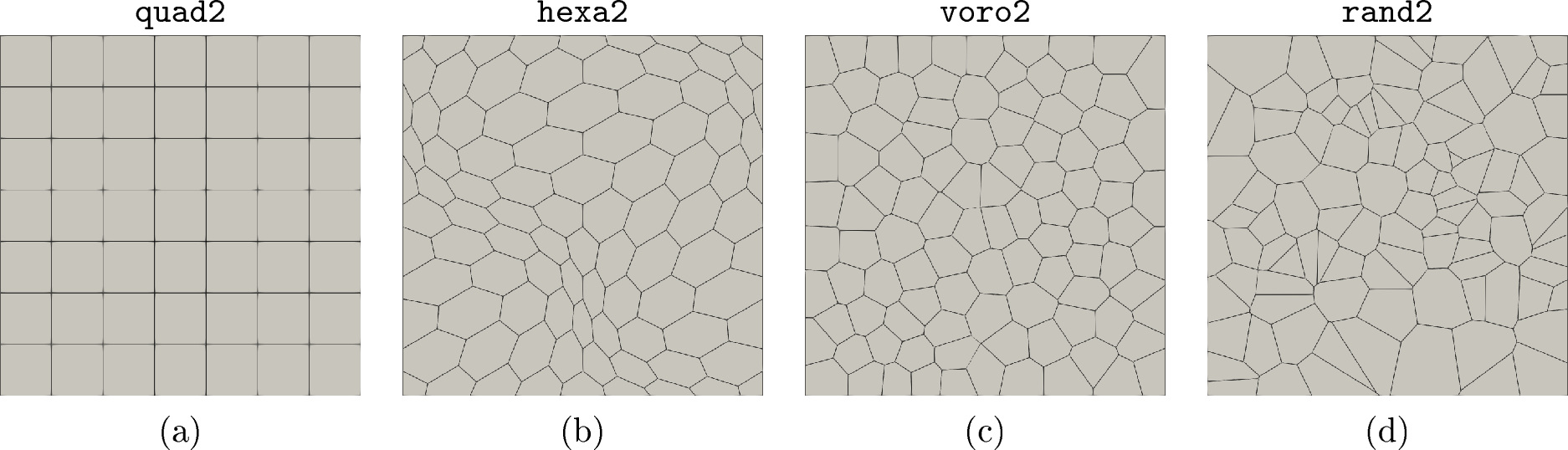
These four types of meshes have an increasing distortion level. The quad one is the most regular. The hexa mesh type has distorted elements but a mostly uniform topology, consisting mainly of hexagons. The voro meshes consist of general polygons with both short and long edges, but they have a regular shape due to the Lloyd optimization. Finally, the rand mesh is the most challenging one, as it contains highly distorted elements and very short edges.

Then, to show the convergence of the errors indicators, we construct four decompositions the unit square \(\Omega=(0,\,1)^2\) with decreasing mesh size \(h\) for each of them. We label these discretizations with the numbers from 1 to 4, 1 will be the coarsest and 4 the finest. For instance voro1 refers to the coarser mesh of the voro type.

For the time discretization, we always consider the time interval \([0,\,1]\) and use uniform time steps. More precisely, we define four temporal partitions, inter1, inter2, inter3, and inter4, corresponding to time steps \(\Delta t = 1/3\), \(1/6\), \(1/12\), and \(1/24\), respectively. For all the simulations we keep the ratio between \(\Delta t\) and \(h\) constant. We set the same approximation degree for both space and time, denoted by \(k\). We compute the errors using the following space–time discretizations: \[(\texttt{mesh1},\texttt{inter1}),\qquad(\texttt{mesh2},\texttt{inter2}),\qquad (\texttt{mesh3},\texttt{inter3}),\qquad\text{and}\qquad(\texttt{mesh4},\texttt{inter4}),\] where mesh* refer to one type of mesh.

In Figure 2, we report the convergence curves corresponding to each mesh type for polynomial degrees 1, 2, and 3. For all space–time approximation degrees, the convergence rates are as expected. Moreover, the curves remain close to each other across different mesh geometries, highlighting the robustness of the proposed method with respect to the element shape. Although the theoretical estimate is not explicitly provided in this paper, we also compute the \(H^1\) seminorm of the error at the final time. This error indicator exhibits the expected convergence rate and, as further evidence of the robustness with respect to the element shape, the convergence curves corresponding to the same approximation degree are very close to each other.

5.1.1 \(k\)-convergence↩︎

In this numerical experiment, we analyze the convergence of the proposed scheme with respect to the space–time approximation degree. To this end, we consider the coarsest space–time discretization, (mesh1, inter1), for each mesh type, and compute both the error indicator err and the \(H^1\) seminorm error at the final time.

In Figure 3, we report the convergence curves. At each refinement in the polynomial degree \(k\), we observe an improvement of approximately one order of magnitude in the error, which is in agreement with the estimate given in Equation ?? .

5.1.2 Robustness with respect to the coefficient \(D\)↩︎

In this section, we analyze the robustness of the proposed method with respect to the diffusion coefficient \(D\). We consider the same setting as before, but we now solve the model problem for different values of \(D\): \[D = [10^{0},\,10^{-1},\,10^{-2},\,10^{-3},\,10^{-4},\,10^{-5},\,10^{-6},\,10^{-7}]\,,\] modifying the data \(\tilde{c}\) and \(c_I\) accordingly. For each value of \(D\), we solve the problem using all mesh types at the second refinement level in both space and time, i.e., (mesh2, inter2).

In Figure 4, we observe that, while keeping the space–time discretization fixed and varying \(D\), the error remains nearly constant. This provides numerical evidence that the proposed method is robust with respect to the diffusion coefficient.

5.2 Multi–species example↩︎

In this section, we apply the proposed method to a multi–species transport problem. The test case is inspired by the Porous Catalytic Reactor with Injection Needle model, available in the open-source COMSOL Multiphysics [34] software and described in detail in [35].

The reactor is a tubular structure, illustrated in Figure 5. The lengths of its parts are proportional to a unit length denoted by . The first species, \(c_1\), is injected from the left side of the tunnel, while the second species, \(c_2\), enters through a tubular inlet positioned on the top. The reactor exhibits a homogeneous distribution of porosity, we set \(\mu K^{-1} = \mathbb{I}\), The diffusion coefficients are set to \(D_1 = D_2 = 0.01\), and the final simulation time is \(T = 20\). For the Darcy problem, we prescribe a constant unit flux at both the inflow and outflow sections of the tube, as illustrated in Figure 5, and impose a zero normal flux condition on the remaining boundaries. For the transport equations, the inflow concentrations of \(c_1\) and \(c_2\) are defined as \[c_1^I(x,y) = y(y-4), \qquad c_2^I(x,y) = (x-2)(4-x)\,,\] respectively.

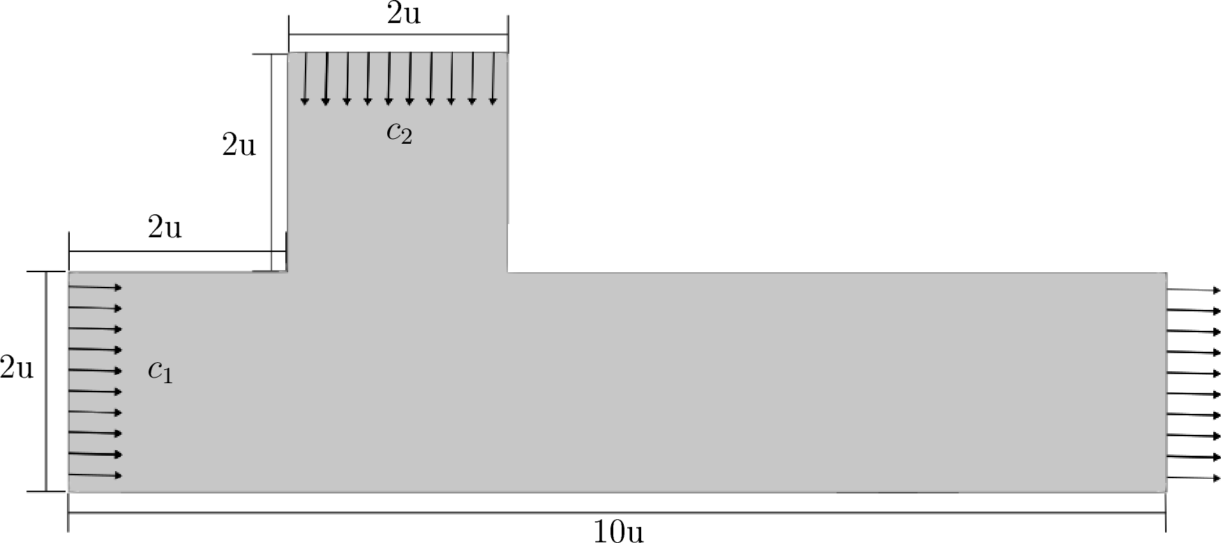
The computational domain is discretized using a Delaunay triangulation, and the time interval is divided into 100 equally spaced sub-intervals. Both the spatial and temporal polynomial degrees are set to one.

Figure 6 shows the flow field obtained from the solution of the Darcy problem, which is consistent with the expected behavior based on the problem data.

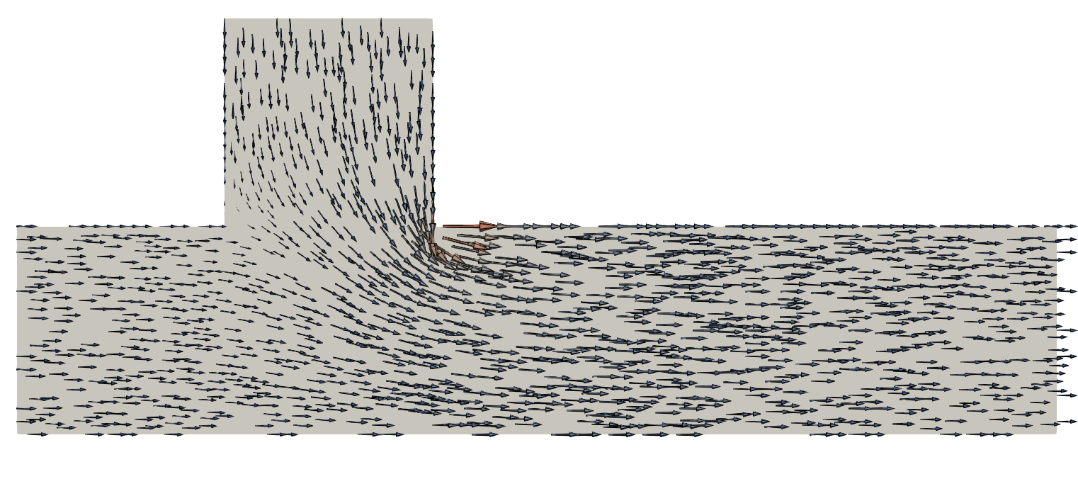
To analyze the impact of the parameters in the first-order reaction term, we fix the degradation rates of the two species to \(\gamma_1 = \gamma_2 = 0.2\). We then consider three different reaction scenarios:

• noReaction: in this case, the two species evolve independently, and the degradation of one species does not generate the other. This behavior is obtained by setting \(y_{1/2} = y_{2/1} = 0.0\);

• lowReaction: in this case, a small amount of \(c_2\) is produced from the degradation of \(c_1\), and vice versa, by setting \(y_{1/2} = y_{2/1} = 0.1\);

• highReaction: here, we consider a non-symmetric case, with a high production of \(c_2\) from \(c_1\), and a low production of \(c_1\) from the degradation of \(c_2\); specifically, \(y_{1/2} = 1.0\) and \(y_{2/1} = 0.1\).

Figures 7 and 8 show selected time steps of the simulations for the three considered scenarios. The results are consistent with the chosen values of the parameters \(y_{*/\circ}\). In both the lowReaction and highReaction cases, a noticeable presence of \(c_2\) is observed along the flow path of \(c_1\), and vice versa. In the lowReaction case, this interaction is roughly symmetric, whereas in the highReaction case the degradation of \(c_1\) produces a significantly higher concentration of \(c_2\). As expected, in the noReaction case no such production is observed for either species.

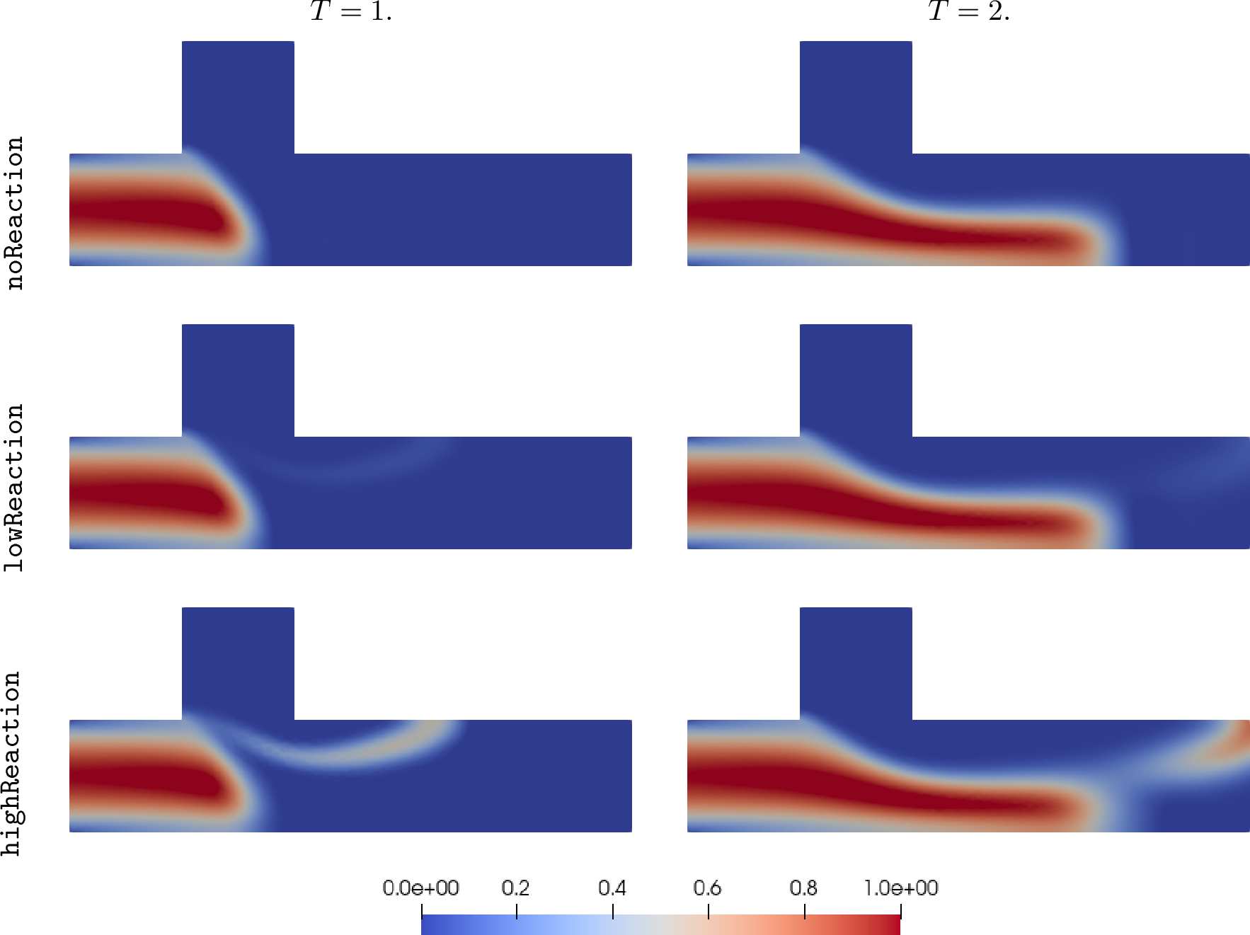
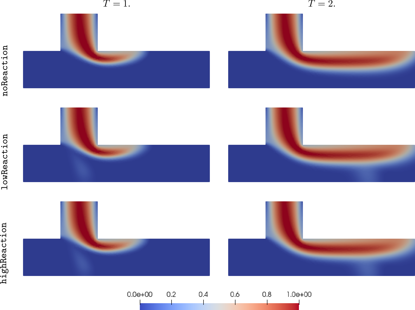
Acknowledgments↩︎

All authors were partially supported by the European Union (ERC Synergy, NEMESIS, project number 101115663) and the Italian Ministry of University and Research (MUR) through the PRIN 2022 project . Views and opinions expressed are, however, those of the authors only and do not necessarily reflect those of the EU or the ERC Executive Agency. The authors would also like to thank Prof. L. Beirão da Veiga and the anonymous referees for their valuable comments and suggestions on the manuscript. FD is also a member of the INdAM-GNCS group.

References↩︎