ELBO-T2IAlign: A Generic ELBO-Based Method for Calibrating Pixel-level Text-Image Alignment in Diffusion Models
June 11, 2025
Abstract
Diffusion models excel at image generation. Recent studies have shown that these models not only generate high-quality images but also encode text-image alignment information through attention maps or loss functions. This information is valuable for various downstream tasks, including segmentation, text-guided image editing, and compositional image generation. However, current methods heavily rely on the assumption of perfect text-image alignment in diffusion models, which is not the case. In this paper, we propose using zero-shot referring image segmentation as a proxy task to evaluate the pixel-level image and class-level text alignment of popular diffusion models. We conduct an in-depth analysis of pixel-text misalignment in diffusion models from the perspective of training data bias. We find that misalignment occurs in images with small-sized, occluded, or rare object classes. Therefore, we propose ELBO-T2IAlign—a simple yet effective method to calibrate pixel-text alignment in diffusion models based on the evidence lower bound (ELBO) of likelihood. ELBO-T2IAlign is training-free and generic: it requires no additional annotations, model retraining, or architectural modifications, and it can be directly applied to different diffusion backbones. Extensive experiments on zero-shot referring image segmentation, text-guided image editing, and compositional image generation verify that the proposed calibration improves pixel-text alignment across complementary downstream tasks.
Diffusion models, text-image alignment, evidence lower bound, referring image segmentation.
1 Introduction↩︎
The rapid advancement of text-to-image (T2I) diffusion models has enabled them to generate unprecedented results from given texts. Recent studies have shown that text-conditional diffusion models can not only generate high-quality images but also encode text-image alignment information [@quangtruong2023dd; @wu2023datasetdm; @wu_diffumask_2023]. This information can be used for various downstream computer vision tasks, including image classification [@li_your_2023; @clark_text--image_2023], object detection [@chen2023diffusiondet], image segmentation [@noauthor_diffusion_2024; @xu_open-vocabulary_2023], and image editing [@hertz_prompt--prompt_2022; @cao_2023_masactrl; @orgad2023editing]. For instance, some research reveals that attention maps in the denoising network encode object semantics [@wang_diffusion_2024; @tang_what_2023]. By effectively reusing these attention maps, diffusion models can be applied to semantic segmentation [@wang_diffusion_2024] and panoptic narrative grounding [@li2024dynamic]. Other studies analyze the diffusion model’s loss function and utilize the loss value for image classification [@li_your_2023; @clark_text--image_2023]. Additionally, text-image alignment information can also be applied to text-guided image editing [@hertz_prompt--prompt_2022; @tumanyan_plug-and-play_2023] and compositional generation [@chefer2023attend; @feng2023training; @rassin2023linguistic]. These downstream applications implicitly assume reliable text-image alignment in the frozen diffusion model, which often fails in practice. Calibrating such misalignment is therefore important for alignment-dependent tasks rather than only for image generation.
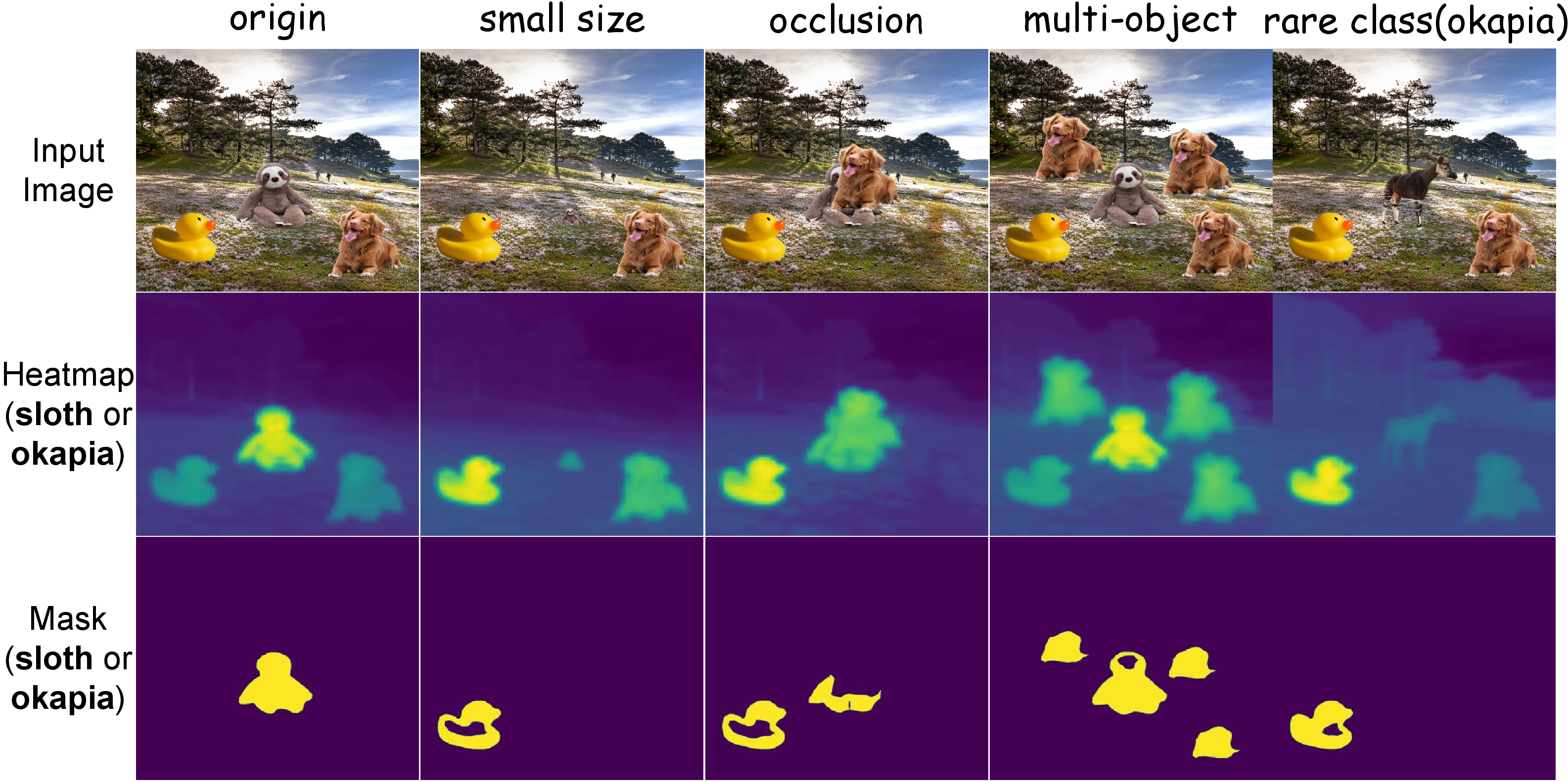
In this paper, we examine the pixel-level image and class-level text alignment using zero-shot referring image segmentation as a proxy task, which can be effectively and quantitatively examined based on off-the-shelf semantic segmentation datasets. We find that one of the key reasons for the imperfect alignment between image pixels and textual classes stems from the biased dataset used for training the diffusion model. In the LAION dataset [@schuhmann2021laion], images are crawled from the internet. However, these internet images are naturally long-tailed due to Zipf’s law of nature [@reed2001pareto], and they mostly contain common object classes rather than rare ones. The long-tailed issue in the LAION dataset has been validated by [@parashar2024neglected; @wen2024generalization].Additionally, each image typically contains only a small number of classes. As a result, the text-image alignment is poorly established when multiple classes are present in a single image. We observe that when multiple classes appear in one image, the misalignment occurs with small-sized, occluded, or rare object classes. Figure 1 illustrates how different data issues affect pixel-text alignment in diffusion models using toy data (please see details in Section 5.1). The poor alignment will lead to inaccurate semantic heatmaps and masks.
To address these issues, we propose ELBO-T2IAlign, a simple yet effective training-free bias correction method to calibrate the pixel-text alignment. This generic approach works without needing to know the exact cause of misalignment, and works well across various diffusion model architectures. Specifically, we define an alignment score based on variational lower bound (ELBO) of the likelihood \(p_{\theta}(x|c)\). Considering an image containing two object classes \(c_1\) and \(c_2\), we claim that \(c_1\) has stronger semantics if \(p_{\theta}(x|c_1)>p_{\theta}(x|c_2)\). We find that diffusion models always focus on classes that have stronger semantics, leading to higher activation values in cross-attention maps. In an image with multiple classes, most classes will have low activation values in cross-attention maps. To obtain ELBO of the log-likelihood, we simply use the diffusion loss functions, which are proved to be written as functions of ELBO [@song_maximum_2021; @kingma_understanding_2023]. Thus, we define the alignment score based on relative conditional diffusion loss values that encode information of ELBO of the log-likelihood. The alignment score corrects the cross-attention maps, ensuring that pixels of all object classes in an image have appropriate cross-attention activation values.
We conduct extensive experiments on three complementary tasks: zero-shot referring image segmentation for pixel-level localization, text-guided image editing for local controllability, and compositional generation for object-level text-image correspondence. The results demonstrate that our ELBO-T2IAlign approach consistently improves pixel-text alignment across different diffusion model architectures.
The contributions of this paper are three-fold:
We propose using zero-shot referring image segmentation as a proxy task to quantitatively evaluate the pixel-level image and class-level text alignment of popular diffusion models.
We conduct an in-depth analysis of pixel-text misalignment in diffusion models from the perspective of training data bias.
We propose ELBO-T2IAlign, a simple yet effective training-free generic method to correct pixel-text misalignment of diffusion models based on the ELBO of likelihood. Extensive experiments verify the effectiveness of our proposed correction approach on segmentation, image editing, and compositional generation.
2 Related Work↩︎
2.1 Diffusion Models↩︎
Diffusion models have emerged as a new state-of-the-art (SOTA) in image and video generation, surpassing the Generative Adversarial Networks (GANs) [@goodfellow2020generative]. These models generate samples by simulating a forward process that transforms data into noise and a reverse process that reconstructs data from noise. The foundational work, DDPM [@ho_denoising_2020], established the framework for diffusion models, while DDIM [@song_denoising_2020] introduced a non-Markovian forward process that accelerates sampling. Latent Diffusion [@rombach_high-resolution_2022] integrates diffusion models with latent variables, improving computational efficiency. Classifier-Free Diffusion Guidance [@ho_classifier-free_2021] provides a conditional classifier that directs models to generate specific categories. ControlNet [@zhang2023adding] introduces control signals for precise image editing. Flow Matching [@papamakarios_normalizing_2021; @lipman_flow_2022] uses optimal transport displacement interpolation to define the conditional probability paths, leading to better performance. Besides, research into diffusion models continues to explore new architectures, such as DiT [@peebles_scalable_2023], which uses Transformers instead of U-Net structures to enhance scalability and efficiency.
2.2 Pixel-text Alignment Using Diffusion Models↩︎
With the exploration and utilization of the attention mechanisms in diffusion models, recent research has focused on exploiting pixel-text alignment of the diffusion models through attention mechanism and applies the alignment nature to downstream tasks like semantic segmentation and image editing. For example, DiffSegmenter [@wang_diffusion_2024] extracts cross-attention maps and self-attention maps, and combines them to achieve zero-shot semantic segmentation. OVAM [@marcos-manchon_open-vocabulary_nodate] and DiffuMask [@wu_diffumask_2023] utilize information from attentions to achieve pixel-level annotation of synthesized images. OVDiff [@noauthor_diffusion_2024] leverages generated data to extract prototype features, thereby utilizing the perception capabilities of diffusion models. DiffSeg [@tian_diffuse_2024] aggregates multi-layer self-attention maps to enable unsupervised segmentation with diffusion models. DiffPNG [@yang_exploring_2024] uses the attention maps from diffusion as a basis, combined with the SAM [@kirillov_segment_2023] model, to generate detailed masks. InvSeg [@yang_exploring_2024] utilizes attention information to extract anchor points, optimizing the latent space and enhancing segmentation accuracy. Differently, PTP [@hertz_prompt--prompt_2022], Shape-Guided Diffusion [@park2024shape], CDS [@nam_contrastive_2024], and SAG [@hong2023improving] utilize attention maps for controllable image editing. However, these methods overlook the training data bias inherent in diffusion models, resulting in suboptimal performance in pixel-image alignment.
3 Preliminary↩︎
3.1 Conditional Diffusion Models↩︎
A conditional diffusion model is a conditional generative model \(p_\theta(x|c)\) that approximates real conditional data distribution \(q(x|c)\). In addition to observed data \(x\), we have a series of latent variables \(z_t\) for timesteps \(t\in[0,1]\). Modern diffusion models process input in latent space. A condition encoder maps condition \(c\) to text embeddings \(\Gamma(c)\in\mathbb{R}^{L\times D_c}\), and an image encoder maps observed data \(x\) to latent \(x_0\in\mathbb{R}^{H_z\times W_z\times D_z}\). The model consists of a forward process and a reverse process. The forward process gradually adds noise to latent \(x_0\), which is a Gaussian diffusion process with marginal distribution \(q(z_t|x_0,c)\): \[z_t = \alpha_{t}x_0+\sigma_{t}\epsilon \;\;\text{where}\;\; t\in[0,1], \epsilon\sim\mathcal{N}(0,I), \label{eq:forward}\tag{1}\] where \(\alpha_{t}\) and \(\sigma_{t}\) are functions of \(t\). The noise schedule (log signal-to-noise ratio) is given by \(\lambda(t)=2\ln(\alpha_{t}/\sigma_{t})\). \(\lambda(t)\) is strictly monotonically decreasing, thus gradually transforming the original \(x_0\) into pure Gaussian noise \(z_1\) in the forward process. The reverse process is given by inverting the forward process using a neural network \(\epsilon_\theta(z_{t},t,c)\).
3.2 ELBO Training Objective↩︎
The ELBO training objective is widely used in early diffusion models [@ho_denoising_2020; @song_denoising_2020], which is equivalent to using KL divergence to directly compare the Gaussian distribution of the reverse process against forward process posteriors. The ELBO training objective of diffusion models is given by [@kingma_variational_2021; @song_maximum_2021]: \[ELB_\lambda(x,c)=\frac{1}{2}\mathbb{E}_{t,\epsilon}[-\frac{\mathrm{d}\lambda}{\mathrm{d}t}\left\|\epsilon_\theta(z_{t},t,c)-\epsilon\right\|_2^2], \label{eq:elbo95formula}\tag{2}\] where \(\lambda\) is the noise schedule given previously. Besides the ELBO objective, recent diffusion models also use different objectives or mixed objectives [@songscore; @lipman_flow_2022; @ho_denoising_2020] instead of the exact ELBO. However, recent work [@kingma_understanding_2023; @esser_scaling_2024] showed that all diffusion training objectives can be formulated as weighted ELBO objectives, which establishes a bridge between recent diffusion losses and the earliest loss function of diffusion models.
4 Method↩︎
In this section, we first define our task setting, analyze the misalignment issues, and outline our motivations. We then present our ELBO-T2IAlign method in detail.
4.0.0.1 Task definition
Given an image \(x\in \mathbb{R}^{H\times W\times C}\) and candidate classes \(\{c_1, \ldots, c_{N}\}\) in caption \(c\), pixel-level image and class-level text alignment can be characterized by \(p_{\theta}(c_i|x_k)\). Here, \(c_i\) indicates the \(i^{th}\) phrase that defines an object class, \(x_k\) represents the \(k^{th}\) pixel in image \(x\), and \(N\) is the number of classes. In an ideal alignment, if the class label of pixel \(x_k\) is \(c_i\), then \(p_{\theta}(c_i|x_k)>p_{\theta}(c_{j\neq i}|x_k)\). We can generate segmentation masks directly using the approximated \(p_{\theta}(c_i|x_k)\). To examine the pixel-text alignment, we employ zero-shot referring image segmentation as a proxy task. Zero-shot RIS aims to segment reference objects \(c_i\) in image \(x\) based on image caption \(c\) without any training data, which can effectively reflect pixel-text alignment.
4.0.0.2 Analyses of misalignment
The misalignment between image pixels and textual classes could be caused by several reasons. We take two classes as an example. According to likelihood and Bayes’ theorem, the posterior is,
\[p_{\theta}(c_1|x_k)=\frac{p(c_1)p_{\theta}(x_k|c_1)}{p(c_1)p_{\theta}(x_k|c_1)+p(c_2)p_{\theta}(x_k|c_2)}.\] Suppose that the class label of \(x_k\) is \(c_1\), an ideal alignment means \(p(c_1)p_{\theta}(x_k|c_1)>p(c_2)p_{\theta}(x_k|c_2)\). However, misalignment happens in at least three cases in practice:
\(p(c_1)\ll p(c_2)\), and \(p_{\theta}(x_k|c_1)>p_{\theta}(x_k|c_2)\)
\(p(c_1)\approx p(c_2)\), and \(p_{\theta}(x_k|c_1)<p_{\theta}(x_k|c_2)\)
\(p(c_1)<p(c_2)\), and \(p_{\theta}(x_k|c_1)<p_{\theta}(x_k|c_2)\)
The first case stems from class imbalance with insufficient training data of \(c_1\) (e.g., rare object classes or small objects present in an image). The second case indicates that even when different classes are approximately balanced, the wrong prediction could still happen due to class confusion between \(c_1\) and \(c_2\), which can occur due to similar visual appearances between \(c_1\) and \(c_2\), or when \(x\) is an out-of-training-distribution sample for class \(c_1\). The third case combines both class imbalance and confusion. In practice, the first case rarely occurs, since the model tends to assign higher likelihoods to classes that appear more frequently in the training data. Therefore, we mainly focus on the second and third cases.
4.0.0.3 Motivation
If the training set is balanced, the likelihoods of different classes \(p_\theta(x|c_i)\) for a given image \(x\) tend to be equal. Introducing two assumptions can ensure reasonably accurate segmentation results: (1) pixels are independent, implying that the image-level likelihood can be factorized into pixel-level likelihoods \(p_\theta(x_k|c_i)\); and (2) the pixel-level likelihood within the target class region is larger than that in the background, enabling object localization. Leveraging the balanced data assumption, Bayes’ rule implies \(p_\theta(c_i|x_k) \propto p_\theta(x_k|c_i)\), which underpins the high-quality segmentation results of diffusion models. However, real-world scenarios suffer from previously discussed issues: imbalanced training sets, out-of-training-distribution (OOD) problems, and class confusion. These issues cause the likelihood of specific classes to dominate, leading to abnormally large pixel-level likelihoods and subsequent missegmentation. Since diffusion models approximate pixel-level likelihoods via cross-attention maps and learn model likelihood via the ELBO objective, we propose leveraging ELBO as a measure of semantic strength. This allows us to calibrate cross-attention maps by heuristically enhancing responses for classes with lower likelihoods, thereby effectively mitigating misalignment.
4.0.0.4 Overview
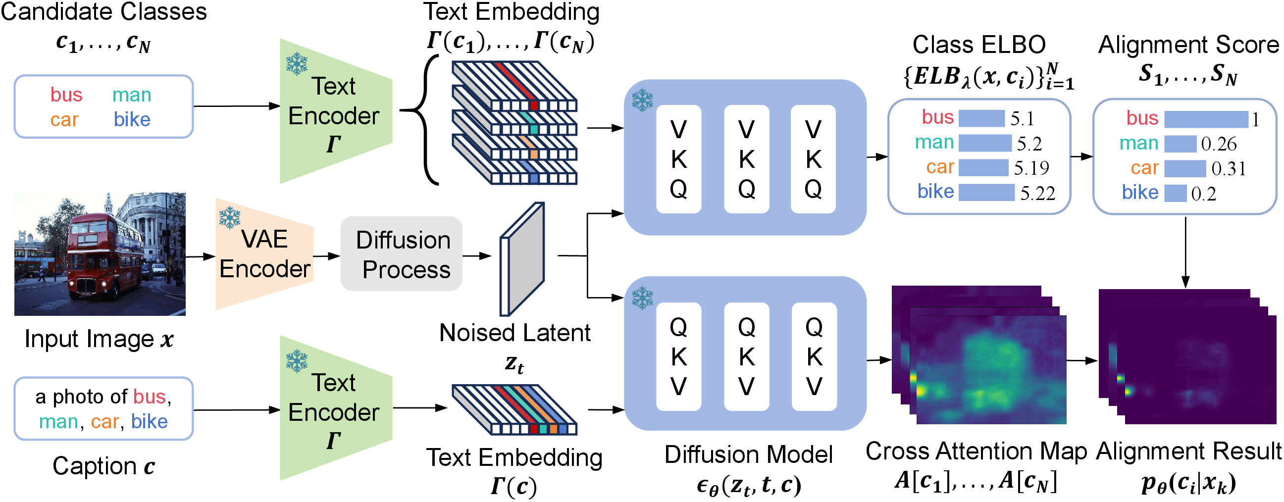
An overview of our method is illustrated in Figure 2. Given a pre-trained frozen diffusion model, we encode the input image \(x\) and caption \(c\) using visual and text encoders, respectively. The visual features undergo noising through the diffusion process. Subsequently, we feed the textual features and noised visual features into the pre-trained denoising model. We approximate the rough pixel-text alignment using the cross-attention map. Then, we compute the ELBO of likelihood \(p_\theta(x|c_i)\) for each class \(c_i\) by passing individual classes as conditions. Based on the ELBO, we define an alignment score, which we use to calibrate the posterior approximated by cross-attention maps.
4.1 Attention-Based Pixel-Text Alignment↩︎
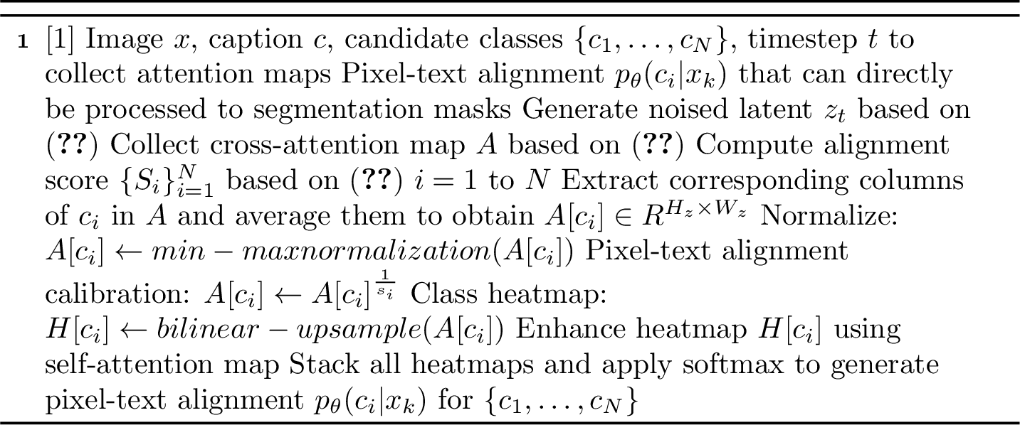
In diffusion models, obtaining the exact \(p_{\theta}(c_i|x_k)\) is intractable. Previous methods approximate it either by the estimated likelihood [@li_your_2023; @clark_text--image_2023] or by using the cross-attention map [@wang_diffusion_2024; @tang_what_2023]. In this paper, we approximate the rough pixel-text alignment \(p_{\theta}(c_i|x_k)\) using the cross-attention map. Our method is applicable to all mainstream diffusion models since they all use attention mechanisms [@NIPS2017_3f5ee243] to condition \(x\) on \(c\) [@hertz_prompt--prompt_2022; @tumanyan_plug-and-play_2023; @rassin2023linguistic]. For transformer-only diffusion models that rely on multi-modal self-attention (SD3, SD3.5, etc.), we split the whole attention map and categorize it into two groups: the text-image cross-attention map and the image-image self-attention map. We collect cross-attention map \(A\) through one forward propagation of \(\epsilon_\theta(z_{t},t,c)\): \[A=softmax(\frac{Q(z_t)K(c)^T}{\sqrt{d}})\in\mathbb{R}^{(H_z\times W_z) \times L}, \label{eq:attention95map}\tag{3}\] where \(d\) is a scaling factor, and \(Q(z_t)\) and \(K(c)\) are visual query and textual key matrices, respectively. Notice that (3 ) only represents one cross-attention layer. In practice, since diffusion models may have multiple cross-attention layers with different resolutions, we resize all cross-attention maps to the same resolution and average them to produce the final \(A\). Interaction between modalities primarily happens in cross-attention [@rombach_high-resolution_2022; @podell_sdxl_2023; @peebles_scalable_2023; @chen2023pixartalpha; @esser_scaling_2024], which computes the similarity between visual query and textual key matrices. Higher cross-attention scores yield larger activation values in \(A\), signifying a stronger relationship between the image pixel and the text label. Therefore, we can approximate \(p_\theta(c_i|x_k)\) by post-processing \(A\). For each candidate class \(c_i\), we first extract the corresponding columns in cross-attention map \(A\) and average these columns to obtain \(A[c_i]\in\mathbb{R}^{H_z\times W_z}\). Then, we apply min-max normalization and bilinear upsampling to \(A[c_i]\), producing heatmap \(H[c_i]\in\mathbb{R}^{H\times W}\). Next, we follow [@wang_diffusion_2024; @xu_mctformer_2023] to further enhance the heatmap \(H[c_i]\) based on the self-attention map that encodes correlations between different pixels. Finally, we generate pixel-text alignment \(p_\theta(c_i|x_k)\) using softmax. The algorithm is the same as Algorithm 3 without Lines 3 and 7.
4.2 Pixel-Text Alignment Calibration with ELBO↩︎
Based on previous discussions, we know pixel-text alignment \(p_\theta(c_i|x_k)\) from cross-attention is inaccurate. One straightforward method to improve the result is explicitly modeling pixel-text alignment, but this approach involves redesigning training objective and training from scratch, which is costly. We propose to leverage ELBO of \(p_\theta(x|c)\) from the pre-trained diffusion models to enhance \(p_\theta(c_i|x_k)\) prediction. As mentioned in the motivation of our method, if an image contains two object classes, we claim that \(c_1\) has stronger semantics if \(p_{\theta}(x|c_1)>p_{\theta}(x|c_2)\). The relative magnitude of ELBO training objective reflects the semantic strengths, and can be used as a signal to instruct the calibration of the attention maps as well as the corresponding approximated \(p_{\theta}(c_i|x_k)\). We introduce an alignment score \(S=\{S_i\}_{i=1}^{N}\) based on ELBO of \(p_{\theta}(x|c_i)\) to identify the semantic strengths of each class in image \(x\): \[S=\gamma^{norm(ELB_\lambda(x,c_1),\ldots,ELB_\lambda(x,c_{N}))}\in\mathbb{R}^{N}, \label{eq:edp95core}\tag{4}\] where \(\gamma \in (0,1]\) is a hyper-parameter. We transform ELBO objective into alignment score \(S_i \in [\gamma,1]\) by applying simple min-max normalization and point-wise exponent, while smaller \(\gamma\) implies larger difference of alignment scores \(\{S_i\}_{i=1}^{N}\). Intuitively, a higher alignment score \(S_i\) indicates that \(c_i\) has stronger semantic relevance, and also suggests that the model tends to misclassify pixels from other classes into this class. With the alignment score, we correct each \(A[c_i]\) by applying an element-wise square root operation with a radical exponent \(S_i\). Our calibration operation can be viewed as heuristically increasing the effective likelihood of classes with lower semantic strength, thus leading to a more reliable approximation of \(p_\theta(c_i\mid x_k)\). The full algorithm is illustrated in Algorithm 3. Because all diffusion training objectives can be formulated as weighted ELBO, we can still estimate the ELBO of \(p_\theta(x|c)\) by “unweighting" different training objectives if we assume \(\theta\) is well learned: \[ELB_{\lambda}(x,c)\approx\frac{1}{2}\mathbb{E}_{t,\epsilon}[\frac{1}{\omega(t)}\mathcal{L}_{\omega,\lambda}(x,t,c)], \label{eq:weight95ELBO}\tag{5}\] where \(\mathcal{L}_{\omega,\lambda}(x,t,c)\) is the single-timestep training objective of diffusion models. We list \(\omega(t)\) of popular training objectives in Table 1, and give the full derivation in the supplementary material. Furthermore, if we assume relative \(\left\|\epsilon_\theta(z_{t},t,c_i)-\epsilon\right\|_2^2\) is stable among candidate classes across all timesteps, then the relative relationship of alignment scores will stay the same when using other objectives to replace \(ELB_\lambda(x,c_i)\).
| Objective | Estimated Function | \(\omega(t)\) | |
|---|---|---|---|
| Score [@songscore] | \(\nabla_{z_t}\text{ln}q(z_{t}|x)\) | \(-1/({\sigma_t^{2}}\cdot\lambda^{'}(t))\) | |
| Flow [@lipman_flow_2022] | \(u(z_{t}|\epsilon)\) | \(-(\sigma_t^{2}\cdot\lambda^{'}(t))/4\) | |
| X [@sohl-dickstein_deep_2015] | \(x\) | \(-1/(\lambda^{'}(t)\cdot e^{\lambda(t)})\) | |
| Epsilon [@ho_denoising_2020] | \(\epsilon\) | \(-1/\lambda^{'}(t)\) | |
| Velocity [@salimans_progressive_2021] | \(\alpha_{t}\epsilon-\sigma_{t}x\) | \(-(\alpha^2_{t}+\sigma^2_{t})^2/(\alpha^2_{t}\cdot\lambda^{'}(t))\) |
5 Experimental Results↩︎
In this section, we use zero-shot referring image segmentation as the primary quantitative proxy for pixel-level localization, and further examine text-guided image editing and compositional generation as complementary tests of local controllability and object-level text-image correspondence.
5.1 Pixel-text Alignment Results↩︎
5.1.0.1 Datasets
We evaluate our approach on the following five datasets. PASCAL VOC 2012 [@everingham2010pascal] contains 20 classes with 1,449 validation images. The PASCAL Context [@mottaghi2014role] dataset includes 5,104 images for validation. We use the 59 most frequent classes, while the others are labeled as background. COCO 2017 [@lin2014microsoft] contains 5,000 images for validation. We use the 80 object classes and set other classes to background. Ade20K [@zhou2019semantic] contains 2,000 images for validation across 150 object and stuff classes. To further verify our method on Attribute-Enriched Prompts, we synthesize a dataset named AEP. AEP contains 38 classes with attribute-enriched image captions (e.g. “three baby rabbits and a pink modern wooden suitcase"). We collect 741 captions from DVMP [@rassin2023linguistic], generating and annotating images with FLUX [@flux2024] and Grounded SAM [@ren2024grounded].
5.1.0.2 Implementation Details
For datasets that do not contain image captions, we concatenate all candidate classes \(\{c_i\}_{i=1}^N\) to produce caption \(c\). For example, if an image contains cat and hot dog classes, the image caption will be “a photo of cat, hot dog". Each candidate class is a noun phrase in the caption, and we generate pixel-text alignment \(p_\theta(c_i|x_k)\) following Algorithm 3. To evaluate the result, we threshold \(p_\theta(c_i|x_k)\), generate a background mask, and label other pixels with the highest probability class. Then, we compare the mask produced by our method with ground truth. We mainly use mean Intersection over Union (mIoU) as the evaluation metric. We use FP16 as default data type to reduce memory usage and accelerate inference. By default, we sample 20 timesteps to compute ELBO and set \(\gamma=1/3\). As observed by DiffSegmenter [@wang_diffusion_2024], different cross-attention layers contain varying degrees of semantic information. Stronger semantic information is captured by lower-resolution cross-attention. We apply a weighted sum to all cross-attention layers, but assign different weights for different resolutions. We empirically use weights \(15,10,1,1\) from the lowest to highest resolution. SDXL has 2 different resolutions, and SD3 has 1 resolution. We use weights \(15,1\) for SDXL and simply average all layers for SD3. More details can be found in supplementary material.
5.1.0.3 Baselines
To verify the effectiveness of the pixel-text alignment enhancement by our method, we compare our method with the state-of-the-art diffusion-based segmentation methods, including DAAM [@tang_what_2023], OVAM [@marcos-manchon_open-vocabulary_nodate], DiffPNG [@yang_exploring_2024], Semantic DiffSeg [@tian_diffuse_2024], and DiffSegmenter [@wang_diffusion_2024]. These methods can be easily adapted to our zero-shot referring image segmentation setting with few or no modifications. To ensure a fair comparison, the seed and text prompt are kept the same across different methods and other parameters are kept at their default values as provided. More details of baselines are in the supplemental material.
5.1.0.4 Quantitative Comparisons with Baseline Methods
Table 2 presents a quantitative comparison of zero-shot referring image segmentation results between our method and other state-of-the-art diffusion-based methods. We evaluate mIoU on four benchmark datasets. Compared to baseline methods, our approach shows significant improvements across different datasets, which demonstrates its strong alignment capability. Our method only performs poorer than DiffSegmenter [@wang_diffusion_2024] on the VOC dataset. We argue that since our method is designed to handle images that have multiple candidate classes, its effectiveness is less pronounced on the VOC dataset with fewer classes in an image.
| Method | mIoU \(\uparrow\) | |||
| VOC | Context | COCO | Ade20K | |
| DAAM [@tang_what_2023] | 48.11 | 26.13 | 29.16 | 15.02 |
| OVAM [@marcos-manchon_open-vocabulary_nodate] | 47.45 | 25.17 | 25.72 | 11.68 |
| DiffPNG [@yang_exploring_2024] | 53.18 | 35.49 | 28.98 | 18.59 |
| DiffSegmenter [@wang_diffusion_2024] | 68.68 | 39.47 | 38.88 | 22.88 |
| Semantic DiffSeg [@tian_diffuse_2024] | 44.34 | 24.29 | 20.34 | 9.80 |
| ELBO-T2IAlign | 68.15 | 43.61 | 42.15 | 26.17 |
5.1.0.5 Qualitative Comparisons with Baseline Methods
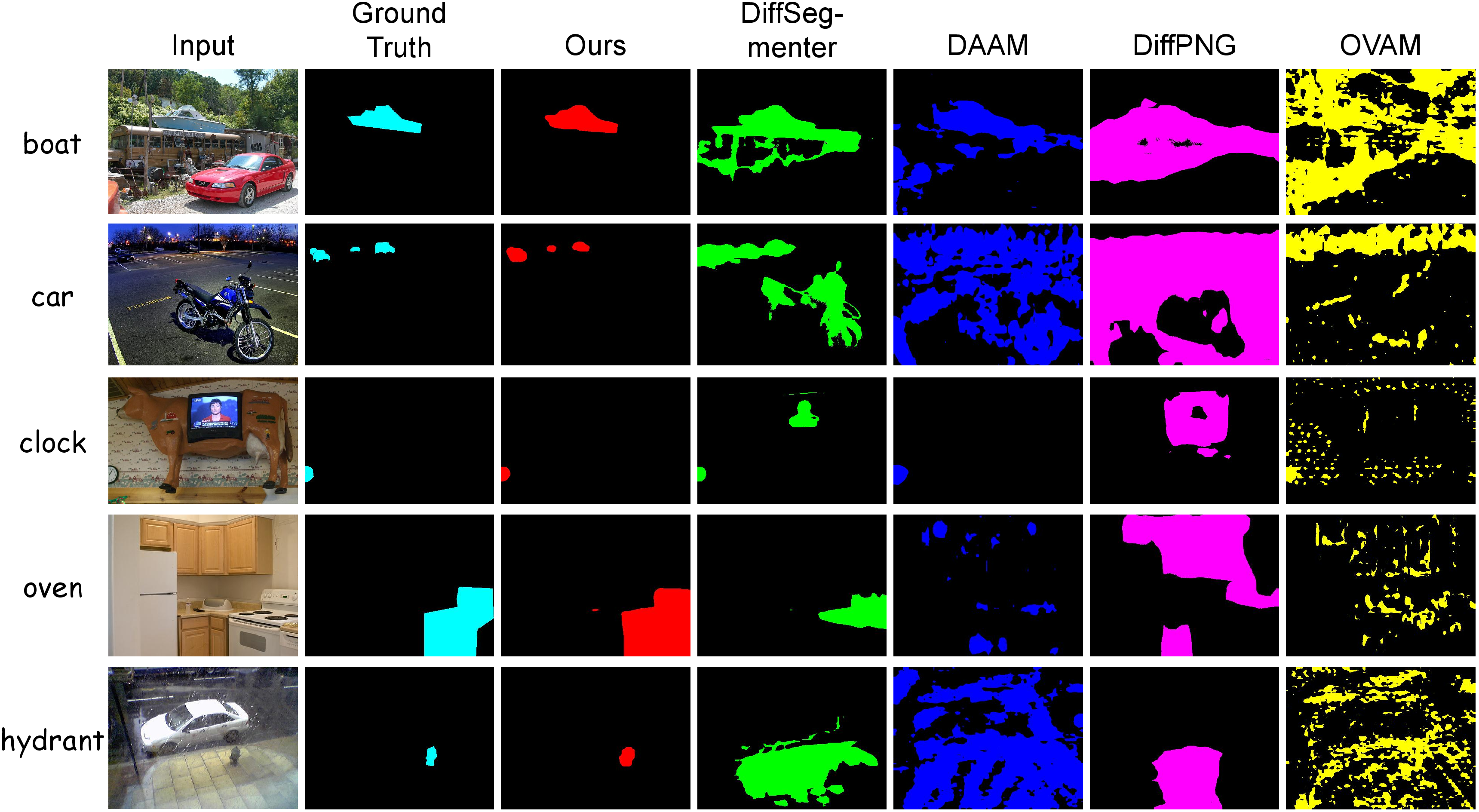
Figure 4 illustrates the qualitative heatmap results comparing our method with other diffusion-based approaches. In the “monitor" case, the monitor appears at the edge of the image and is only partially visible. In the”sink" case, the sink occupies a very small portion of the image. In the “water" case, water is a background element that is not easily recognizable compared to other objects, making intentional localization challenging. In the”chair" case, the chair is obstructed by people and only the backrest is visible. The results indicate that our method achieves more precise localization and object contour capture for small objects like the sink, incomplete or obstructed objects like the monitor and chair, and less recognizable objects like water, compared to other methods. This demonstrates that our approach can better capture the semantic information of small or less prominent objects in multi-object scenes, reducing semantic confusion between different classes. We also present some segmentation masks generated by our method and other diffusion-based approaches in Figure 5.

5.1.0.6 Pixel-text Alignment Examination on Toy Data
We conduct several toy experiments to examine how the semantic strength in an image affects the pixel-text alignment from pre-trained diffusion models. We observe at least four types of operations that reduce the semantic strength: small size, occlusion, multi-object, and rare class. Small size refers to proportionally scaling down an object, occlusion indicates occluding part of the object, multi-object refers to creating multiple copies of background objects, and rare class means replacing an object with a rarely seen object. We produce heatmaps and masks using Algorithm 3 without Lines 3 and 7. As shown in Figure 1, compared to the “original" image, the pixel-text alignment of the targeted sloth plushie is weakened when its size is reduced, when occlusion occurs, or when multiple irrelevant objects are present. If we replace the target sloth plushie with a rare object (okapia), which has limited training data, the pixel-text alignment is also poor.
5.1.0.7 ELBO-T2IAlign Results of Various Diffusion Models
| Model | ELB | mIoU \(\uparrow\) | |||
| VOC | Context | COCO | Ade20K | ||
| SD1.4 | 67.79 | 40.80 | 38.74 | 23.42 | |
| SD1.4 | \(✔\) | 68.22 | 43.59 | 41.80 | 26.85 |
| SD1.5 | 67.57 | 40.61 | 39.19 | 22.66 | |
| SD1.5 | \(✔\) | 68.15 | 43.61 | 42.15 | 26.17 |
| SD2 | 63.71 | 37.39 | 39.60 | 22.65 | |
| SD2 | \(✔\) | 64.96 | 39.31 | 43.64 | 26.04 |
| SD2.1 | 67.6 | 40.70 | 41.37 | 23.41 | |
| SD2.1 | \(✔\) | 69.04 | 42.41 | 44.53 | 26.32 |
| SDXL | 57.72 | 33.28 | 34.89 | 17.87 | |
| SDXL | \(✔\) | 58.40 | 35.70 | 36.43 | 19.28 |
| SD3.5 | 51.17 | 36.23 | 35.25 | 22.54 | |
| SD3.5 | \(✔\) | 51.74 | 37.27 | 37.31 | 25.01 |
To demonstrate the generic nature of our method, we conduct experiments on diffusion models with different training objectives and architectures. The results are shown in Table 3. It is evident that across all tested models whose training objectives are different, ELBO-T2IAlign consistently improves performance. This consistent improvement suggests that our refined strategy contributes significantly to the model alignment capability, regardless of the specific training objective and architecture of the model.
5.1.0.8 ELBO-T2IAlign Results on Datasets with Attribute-enriched Prompts
Since alignment score \(S\) is the core of our method, we conduct experiments on generating \(S\) with different strategies. Specifically, we are interested in whether using a whole noun phrase (e.g. “a golden dog") is better than using a single noun (e.g. ”dog") in (4 ). When computing alignment score \(S\), does more accurate textual input lead to better results? We show the results on our AEP dataset in Table 4. The results show that using the whole noun phrase as a candidate class is better than using a single noun. Using more accurate textual input is beneficial, which is consistent with recent methods that use a prompt enhancement module before generation.
| Model | Setting | mIoU \(\uparrow\) | Prec \(\uparrow\) | F1 Score \(\uparrow\) |
|---|---|---|---|---|
| SD1.5 | w/o ELB | 58.70 | 68.77 | 72.62 |
| SD1.5 | ELB | 60.11 | 71.38 | 73.89 |
| SD1.5 | ELB with AE | 60.58 | 71.66 | 74.18 |
| SDXL | w/o ELB | 52.55 | 64.29 | 67.53 |
| SDXL | ELB | 53.81 | 66.33 | 68.95 |
| SDXL | ELB with AE | 53.82 | 66.96 | 68.86 |
| SD3.5 | w/o ELB | 52.63 | 64.05 | 67.76 |
| SD3.5 | ELB | 52.46 | 65.31 | 67.77 |
| SD3.5 | ELB with AE | 52.90 | 65.13 | 68.16 |
5.2 Results on Image Generation and Editing↩︎
5.2.0.1 Compositional Image Generation
| Method | Model | CLIP score \(\uparrow\) | ||
| A&E | DVMP | ABC-6K | ||
| Baseline | SD1.5 | 31.45 | 32.33 | 32.73 |
| A&E [@chefer2023attend] | SD1.5 | 33.09 | 32.24 | 32.48 |
| SynGen [@rassin2023linguistic] | SD1.5 | 31.83 | 32.18 | 32.45 |
| ELBO-T2IAlign | SD1.5 | 32.70 | 33.43 | 33.27 |
| Baseline | SD2.1 | 32.51 | 32.83 | 32.98 |
| A&E [@chefer2023attend] | SD2.1 | 33.62 | 33.16 | 32.86 |
| SynGen [@rassin2023linguistic] | SD2.1 | 32.20 | 32.34 | 32.70 |
| ELBO-T2IAlign | SD2.1 | 33.24 | 33.49 | 33.30 |
| Baseline | SDXL | 33.61 | 34.27 | 33.22 |
| ELBO-T2IAlign | SDXL | 33.72 | 34.45 | 33.37 |
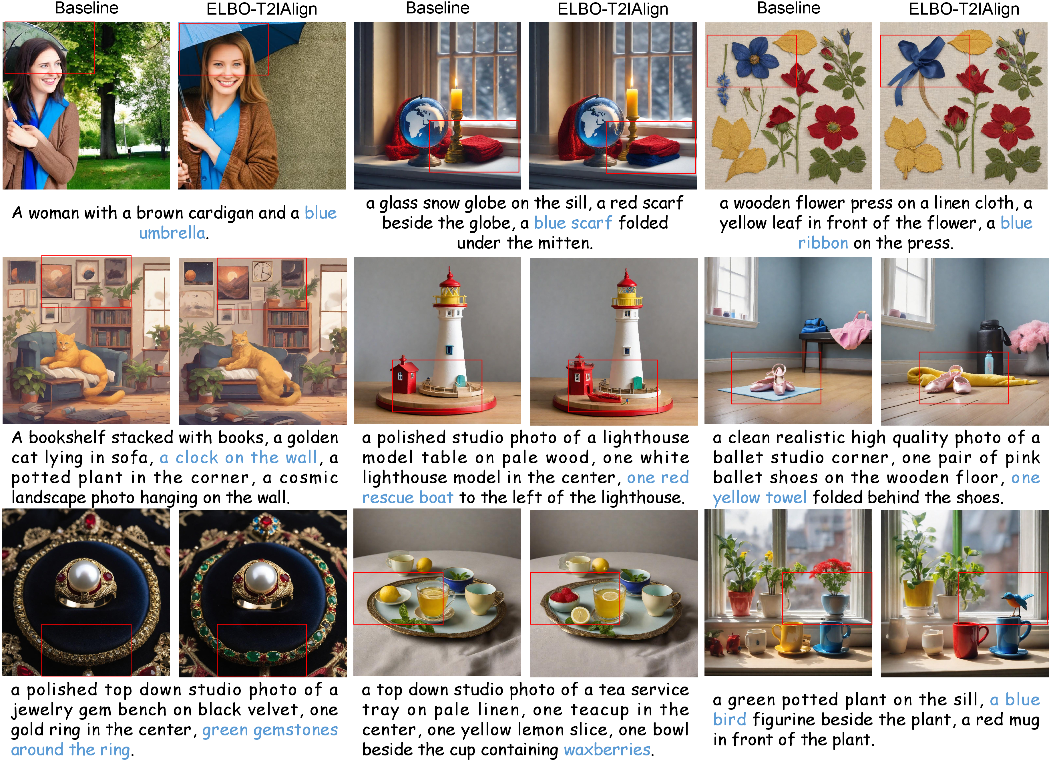
Our method can improve compositional generation using the proposed alignment score \(S\). Given caption \(c\), we extract entities and their visual attributes to obtain \(\{c_i\}_{i=1}^N\). For each denoising step, we first estimate \(\epsilon\) using \(\epsilon_\theta(z_t,t,c)\). Then, we follow (2 ) and (4 ) to estimate \(S\). Finally, we use \(S\) for prompt reweighting [@damian0815_compel; @wang_diffusion_2024] to balance the semantics of \(\{c_i\}_{i=1}^N\) and estimate \(\epsilon\) with the reweighted prompt to denoise the latent. Specifically, when alignment score \(S_{i}\) is low, we increase the weight of class \(c_i\). Balanced semantics allow the generated image to better represent extracted entities, thus improving text-image alignment. Following a recent method [@rassin2023linguistic], we evaluate our method on the A&E [@chefer2023attend], DVMP [@rassin2023linguistic], and ABC-6K [@feng2023training] datasets using CLIP score. Compositional generation methods have two input settings: text-only input (A&E [@chefer2023attend], SynGen [@rassin2023linguistic]) and additional layout input (BeYourself [@0Be]). Our method is designed for text-only input. We compare our method with text-only input methods in Table 5 and visualize some images in Figure 6. A&E and SynGen are coupled with the model architecture, so we do not implement them for the SDXL series or tune their hyper-parameters. The results show that our ELBO-T2IAlign method consistently improves text-image alignment over the baselines. We provide full details and more experimental results in the supplementary material.
5.2.0.2 Text Guided Image Editing
Various diffusion-based image editing methods are based on cross-attention manipulation. Because ELBO-T2IAlign calibrates these maps, it can also improve local text-guided editing control. Specifically, we use PTP [@hertz_prompt--prompt_2022] as baseline, which injects source text cross-attention to target text cross-attention to achieve editing. Given source text \(c\), we extract entities and their visual attributes to obtain \(\{c_i\}_{i=1}^N\). Then, we generate heatmaps of source text following Algorithm 3. Next, we scale these heatmaps based on source text cross-attention and use the scaled heatmaps to replace target text cross-attention. The visualization results are shown in Figure 7. Our method can achieve editing more accurately with the scaled heatmaps. We give more results in the supplementary.
![Figure 7: Comparison results of image editing based on PTP [@hertz_prompt--prompt_2022] before and after calibration using our ELBO-T2IAlign.](/article/2506.09740/img/edit_maintex_compare.png "fig:")
5.3 Further Analyses↩︎
5.3.0.1 Analysis of Computational Resources Cost
We primarily employ Python 3.11.9, PyTorch 2.5.1, transformers 4.51.3 [@wolf-etal-2020-transformers], and diffusers 0.33.1 [@von-platen-etal-2022-diffusers] to implement our method on a single Ubuntu 20.04.3 LTS server with NVIDIA RTX 4090 graphics cards. Memory usage of our method is very close to model forward propagation, because we only perform forward propagation when computing ELBO and collecting attention maps. Our method uses approximately 7 GB of memory for Stable Diffusion v1/v2 and approximately 13 GB of memory for Stable Diffusion XL. For an image with 10 classes, our method takes around 4 seconds to generate all final masks on a single NVIDIA RTX 4090 graphics card with Stable Diffusion v1.5. The additional cost mainly comes from forward-only denoiser evaluations for estimating class-wise ELBO scores; no gradient computation, optimization, retraining, extra annotations, or architectural modifications are required. The timestep ablations show that the cost can be controlled by reducing the number of sampled timesteps when a faster setting is needed. If more GPU memory is available, our method can compute ELBO for all classes in a single batch to accelerate inference.
5.3.0.2 Effect of the Number of Timesteps to Compute ELBO
To calculate ELBO, we sample timesteps evenly in the range \([0,1]\). In Table 6, we demonstrate the impact of sampled timesteps by varying \(\text{ELBO Timesteps} \in \{1,5,20\}\) while keeping other hyperparameters unchanged. We find that as the number of sampling points increases, the mIoU on each dataset shows an upward trend. However, this increase is gradual, and inference time rises with more sampling points. Therefore, we balance these factors and choose \(\text{ELBO Timesteps}=20\) as the default number of sampling steps for ELBO computation in our main experiment. We give more results in supplementary material.
| Method | Steps | mIoU \(\uparrow\) | |||
| VOC | Context | COCO | Ade20K | ||
| SD1.5 | 1 | 67.35 | 40.58 | 39.80 | 24.58 |
| SD1.5 | 5 | 68.15 | 42.28 | 41.36 | 24.93 |
| SD1.5 | 20 | 68.15 | 43.61 | 42.15 | 26.17 |
| SD2 | 1 | 63.00 | 35.63 | 40.32 | 23.57 |
| SD2 | 5 | 63.50 | 38.21 | 42.57 | 24.65 |
| SD2 | 20 | 64.96 | 39.31 | 43.64 | 26.04 |
| SDXL | 1 | 56.58 | 33.05 | 34.75 | 17.94 |
| SDXL | 5 | 58.14 | 34.43 | 36.01 | 18.73 |
| SDXL | 20 | 58.40 | 35.70 | 36.43 | 19.28 |
| SD3 | 1 | 54.56 | 38.99 | 37.26 | 27.04 |
| SD3 | 5 | 54.03 | 39.64 | 37.37 | 28.05 |
| SD3 | 20 | 55.14 | 40.02 | 37.76 | 27.52 |
| SD3.5 | 1 | 51.36 | 36.11 | 36.02 | 22.99 |
| SD3.5 | 5 | 51.55 | 36.62 | 35.98 | 23.90 |
| SD3.5 | 20 | 52.04 | 36.51 | 36.44 | 23.77 |
5.3.0.3 Effect of Sampling Strategy to Compute ELBO
The definition of ELBO suggests that timesteps should be sampled uniformly for ELBO computation. We investigated whether alternative sampling strategies could yield better results. We present the results of different sampling strategies for ELBO computation in Table 7. For the “Small",”Middle", and “Large" strategies, we sample timesteps evenly from \([0, 0.2]\), \([0.4, 0.6]\), and \([0.7, 0.9]\), respectively. For the”Random" strategy, we sample timesteps randomly from \([0,1]\). For the “Even" strategy, we sample timesteps evenly from \([0,1]\). We use 10 timesteps for all sampling strategies to ensure a fair comparison. The results align with our theoretical predictions. The”Random" strategy is the best for computing alignment score, followed by the “Even" strategy. Since these two strategies yield similar results, we adopt the”Even" strategy as default to reduce the randomness of our method. Comparing the results of the “Small",”Middle", and “Large" strategies reveals that larger timesteps experimentally improve ELBO computation, which may be related to the noise schedule \(\lambda(t)\).
| Model | Strategy | mIoU \(\uparrow\) | |||
| VOC | Context | COCO | Ade20K | ||
| SD1.5 | Small | 67.07 | 40.93 | 39.55 | 23.27 |
| SD1.5 | Middle | 68.16 | 42.68 | 41.34 | 25.84 |
| SD1.5 | Large | 68.80 | 42.97 | 41.46 | 25.79 |
| SD1.5 | Random | 68.34 | 43.21 | 41.86 | 26.15 |
| SD1.5 | Even | 68.18 | 43.21 | 41.62 | 26.08 |
| SD2 | Small | 62.67 | 34.69 | 39.93 | 22.25 |
| SD2 | Middle | 62.57 | 35.54 | 41.48 | 25.06 |
| SD2 | Large | 62.74 | 36.94 | 41.91 | 25.59 |
| SD2 | Random | 63.54 | 37.18 | 42.61 | 25.91 |
| SD2 | Even | 63.38 | 37.35 | 42.10 | 25.61 |
| SDXL | Small | 51.70 | 19.70 | 24.87 | 8.78 |
| SDXL | Middle | 52.19 | 20.21 | 25.40 | 9.97 |
| SDXL | Large | 52.76 | 20.37 | 25.33 | 9.85 |
| SDXL | Random | 52.77 | 21.09 | 25.43 | 9.96 |
| SDXL | Even | 52.87 | 20.77 | 25.63 | 9.88 |
| SD3 | Small | 53.36 | 38.39 | 37.61 | 26.14 |
| SD3 | Middle | 54.57 | 39.86 | 38.17 | 26.90 |
| SD3 | Large | 54.55 | 40.27 | 37.52 | 28.47 |
| SD3 | Random | 54.53 | 39.98 | 37.59 | 26.68 |
| SD3 | Even | 54.58 | 39.99 | 37.47 | 27.71 |
5.3.0.4 Evaluations of Different \(\gamma\)
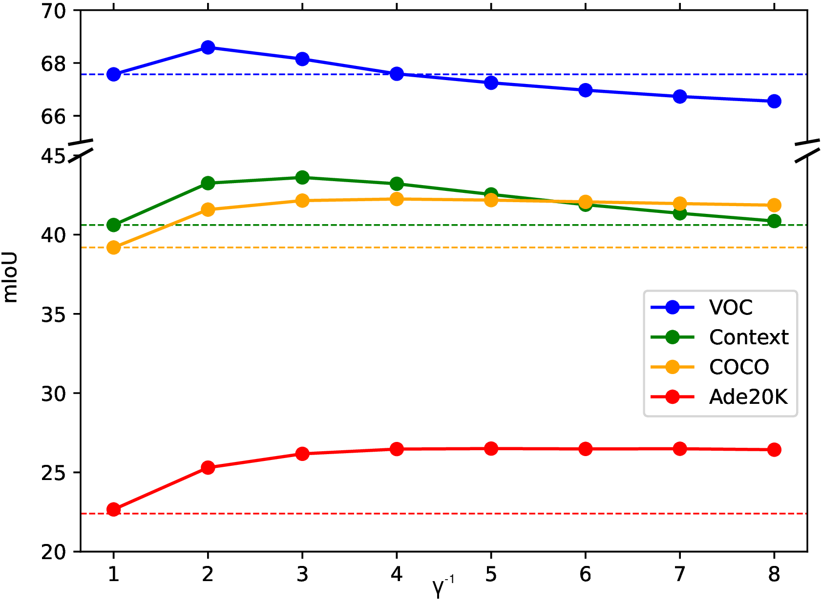
In our method, \(\gamma\) in (4 ) is a critical hyperparameter that directly affects the ability of the ELBO to calibrate pixel-text alignment. An inappropriate value of \(\gamma\) can even worsen pixel-text alignment. Therefore, we varied \(\gamma^{-1} \in \{1,2,3,4,5,6,7,8\}\) to observe its impact on mIoU. Our results show that the performance generally improves as \(\gamma\) decreases from \(1\) to around \(1/2\) or \(1/3\), but further decreases in \(\gamma\) tend to either plateau or result in a slight decline. This suggests that \(\gamma=1/2\) or \(\gamma=1/3\) will be the best choice. In our main experiment, we choose \(\gamma=1/3\) as the default value. We show the pixel-text alignment results on four benchmark datasets in Figure 8. To demonstrate that the effect is not due to the sqrt function itself, we fix alignment score \(\{S_i\}_{i=1}^N\) on line 7 of Algorithm 3. We set alignment score of each class to the same constant. As Table 8 shows, the results are better when ELBO is in effect.
| Method | Alignment Score \(S\) | mIoU \(\uparrow\) | |||
| VOC | Context | COCO | Ade20K | ||
| SD1.5 | \(S=\bm{1/2}\) | 66.61 | 40.29 | 40.13 | 22.90 |
| SD1.5 | \(S=\bm{1/3}\) | 65.11 | 39.72 | 40.09 | 23.04 |
| SD1.5 | \(S=\bm{1/4}\) | 63.28 | 38.69 | 39.58 | 22.87 |
| SD1.5 | ELB based \(S\) | 68.15 | 43.61 | 42.15 | 26.17 |
| SD2 | \(S=\bm{1/2}\) | 61.09 | 35.50 | 39.43 | 21.83 |
| SD2 | \(S=\bm{1/3}\) | 58.45 | 33.22 | 38.97 | 21.24 |
| SD2 | \(S=\bm{1/4}\) | 55.64 | 31.09 | 38.32 | 20.38 |
| SD2 | ELB based \(S\) | 64.96 | 39.31 | 43.64 | 26.04 |
| SDXL | \(S=\bm{1/2}\) | 57.21 | 33.05 | 35.70 | 18.30 |
| SDXL | \(S=\bm{1/3}\) | 55.99 | 32.78 | 35.82 | 18.55 |
| SDXL | \(S=\bm{1/4}\) | 54.39 | 32.49 | 35.58 | 18.75 |
| SDXL | ELB based \(S\) | 58.40 | 35.70 | 36.43 | 19.28 |
5.3.0.5 Effect of Different Attention Collecting Timesteps
| Model | Steps | Strategy | mIoU \(\uparrow\) | |||
| VOC | Context | COCO | Ade20K | |||
| SD1.5 | 1 | Small | 67.97 | 42.38 | 41.41 | 25.92 |
| SD1.5 | 10 | Small | 68.18 | 43.21 | 41.62 | 26.08 |
| SD1.5 | 10 | Middle | 57.77 | 40.61 | 30.78 | 22.42 |
| SD1.5 | 10 | Large | 37.69 | 27.47 | 18.72 | 14.27 |
| SD1.5 | 10 | Random | 51.95 | 35.95 | 27.17 | 19.62 |
| SD2 | 1 | Small | 62.52 | 39.56 | 37.37 | 23.27 |
| SD2 | 10 | Small | 64.62 | 39.06 | 43.09 | 25.43 |
| SD2 | 10 | Middle | 63.50 | 40.29 | 37.38 | 23.51 |
| SD2 | 10 | Large | 44.25 | 31.32 | 23.43 | 16.89 |
| SD2 | 10 | Random | 56.49 | 37.65 | 32.13 | 21.94 |
| SD3 | 1 | Small | 54.60 | 39.04 | 37.62 | 26.14 |
| SD3 | 10 | Small | 54.55 | 39.98 | 37.47 | 26.90 |
| SD3 | 10 | Middle | 53.38 | 42.49 | 35.00 | 30.17 |
| SD3 | 10 | Large | 39.32 | 32.37 | 22.54 | 20.42 |
| SD3 | 10 | Random | 46.41 | 38.14 | 29.46 | 26.18 |
| SD3 | 10 | Even | 49.43 | 40.13 | 32.81 | 27.68 |
For simplicity, we only select one timestep \(t\) in Algorithm 3 to demonstrate our calibration process. In practice, we select multiple timesteps to generate pixel-text alignment results and average them. Different timesteps represent different stages in the diffusion process, with each timestep value affecting the data generated during inference. Both cross-attention and self-attention maps—which are fundamental to obtaining the final mask—are significantly influenced by timesteps, which in turn affect pixel-text alignment. To examine how timesteps influence pixel-text alignment during mask generation, we experiment with different timestep values while maintaining all other hyperparameters constant. To obtain attention maps, we sample timesteps evenly within specific ranges. The parameter “Steps" in Table 9 indicates the number of sampling timesteps and the”Strategy" defines the specific sampling range: “Small" corresponds to \([0,0.2]\),”Middle" corresponds to \([0.4,0.6]\), “Large" corresponds to \([0.7,0.9]\), and”Random" means random sampling from the range \([0,1]\). Table 9 demonstrates that the sampling range of timesteps significantly affects pixel-text alignment. Larger timesteps introduce more noise, which disrupts the original image information and leads to poorer alignment performance. Small timesteps barely alter the visual information contained in the image. Based on these findings, we set Steps=\(10\) and use the range \([0,0.2]\) as our default values in the main experiment.
5.3.0.6 Analysis of Class Imbalance Effects
To assess the impact of training data distribution, we estimate the occurrence probability of object categories by counting their frequencies within a random 16-million sample of the LAION dataset [@schuhmann2021laion] via regular expression matching. Unlike VOC or Context, COCO and Ade20K exhibit significant long-tail distributions, making them suitable for analyzing data bias. We stratify categories into Rare, Common, and Frequent groups based on frequency tertiles (33rd and 66th percentiles). As shown in Table 10, the baseline model (SD1.5 without ELB) exhibits a significant performance disparity between “Common" and”Rare" categories. This confirms that data bias leads to text-image misalignment, particularly for underrepresented objects. After applying ELBO-T2IAlign, we observe consistent improvements across all frequency groups on both benchmarks, showing that the proposed calibration is effective in most cases where the frozen model still provides usable but biased alignment responses. This indicates that our method effectively mitigates the text-image misalignment stemming from data bias.
| Dataset | ELB | mIoU \(\uparrow\) | ||
| Rare | Common | Frequent | ||
| COCO | 31.39 | 46.09 | 40.34 | |
| \(✔\) | 33.63 | 50.25 | 43.07 | |
| Ade20k | 18.93 | 23.15 | 25.60 | |
| \(✔\) | 23.64 | 27.62 | 28.47 | |
5.4 Limitation↩︎
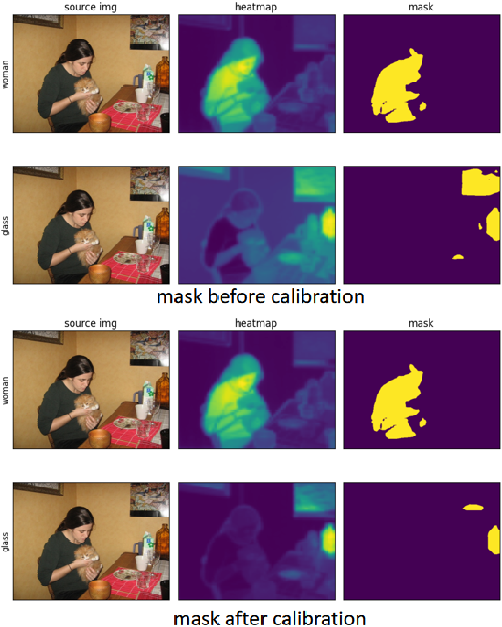
Most evaluated cases fall into the common setting where the frozen model provides weak or biased but usable attention responses, which ELBO-T2IAlign can calibrate effectively. While our ELBO-T2IAlign demonstrates effectiveness in calibrating pixel-text alignment, our method relies on the intrinsic recognition capability of the frozen diffusion model. As a calibration approach, it re-weights existing cross-attention signals rather than generating new ones. Consequently, if the base model completely fails to activate the attention map for a specific object (e.g., failing to recognize “glass", resulting in zero activation, information mix-up [@chen2024cat]), our method cannot recover the missing mask. A concrete example is illustrated in Figure 9. The model successfully segments the”woman" based on valid attention signals. Conversely, the “glass" on the table lacks any initial activation, resulting in a failure to generate a correct mask in both the baseline and our calibrated results. Exploring this limitation represents an interesting direction for future work.
6 Conclusions↩︎
Our research introduces a novel training-free and generic approach called ELBO-T2IAlign, which leverages the evidence lower bound (ELBO) of likelihood to correct pixel-text misalignment in pre-trained diffusion models. We evaluated the alignment capabilities of popular diffusion models and uncovered the training data biases that lead to misalignment, particularly in images with small, occluded, or rare class objects. Our proposed method offers an effective alignment calibration solution that is agnostic to the underlying cause of misalignment and compatible with diverse diffusion model architectures. The results indicate that ELBO-T2IAlign calibrates a shared pixel-text alignment signal rather than targeting only a single downstream behavior. Its training-free and architecture-agnostic nature makes it practically applicable to different frozen diffusion backbones without additional annotations, retraining, or model modifications. This work paves the way for more effective downstream tasks in image segmentation, image editing, and controllable generation. This work relies on the accuracy of the ELBO likelihood estimated by pre-trained diffusion models. Nevertheless, despite this imperfect estimation, our method consistently improves performance.
Acknowledgments↩︎
This work was supported in part by National Natural Science Foundation of China (No.62461160331, No.62132001, No.62572039), in part by Huawei-BUAA Joint Lab, in part by the NSFC/RGC Collaborative Research Scheme (CRS_HKU703/24). Dr. Xu’s research work described in this paper was conducted in the JC STEM Lab of Multimedia and Machine Learning funded by The Hong Kong Jockey Club Charities Trust.
*Corresponding author↩︎
Qin Zhou, Zhiyang Zhang, Jinglong Wang, Jing Zhang, Qian Yu, Lu Sheng are with the School of Software, Beihang University, Beijing 100191, China (e-mail: zhouqin2023@buaa.edu.cn, 20377279@buaa.edu.cn, wjlzy@buaa.edu.cn, zhang_jing@buaa.edu.cn).↩︎
Xiaobin Li is with the College of Computer and Cyber Security, Hebei Normal University, Hebei 050024, China (e-mail: lixiaobin@buaa.edu.cn).↩︎
Dong Xu is with the Department of Computer Science, The University of Hong Kong, Hong Kong (e-mail: dongxu@hku.hk).↩︎
Manuscript received April 19, 2021; revised August 16, 2021.↩︎