Generalized Fisher-Weighted SVD: Scalable Kronecker-Factored Fisher Approximation for Compressing Large Language Models
May 23, 2025
Abstract
The Fisher information is a fundamental concept for characterizing the sensitivity of parameters in neural networks. However, leveraging the full observed Fisher information is too expensive for large models, so most methods rely on simple diagonal approximations. While efficient, this approach ignores parameter correlations, often resulting in reduced performance on downstream tasks. In this work, we mitigate these limitations and propose Generalized Fisher-Weighted SVD (GFWSVD) — a post-training LLM compression technique that accounts for both diagonal and off-diagonal elements of the Fisher information matrix, providing a more accurate reflection of parameter importance. To make the method tractable, we introduce a scalable adaptation of the Kronecker-factored approximation algorithm for the observed Fisher information. We demonstrate the effectiveness of our method on LLM compression, showing improvements over existing compression baselines.
1 Introduction↩︎
The Fisher information Fisher Information Matrix (FIM) [1] is widely employed in neural networks to enhance the efficiency of models, particularly in the context of training and inference. However, computing and leveraging the full Fisher information is computationally prohibitive for deep networks. To make the problem tractable, existing methods adopt simplified approximations – most commonly, assuming that the Fisher matrix is diagonal [2]–[4]. While efficient, this assumption discards valuable information about parameter correlations.
One key application of FIM is low-rank compression of large language models (LLMs). However, the standard low-rank approach — Singular Value Decomposition (SVD) — often leads to suboptimal performance. To mitigate this, weighted SVD methods aim to align the optimization objective with the target task [5], [6]. Fisher-Weighted SVD (FWSVD) [6] uses Fisher information to assign importance to parameters. However, FWSVD utilizes only the diagonal part of FIM and treats each row as independent, which can lead to poor retention of task-critical components.
In contrast, we propose a more accurate weighted SVD method: Generalized Fisher-Weighted SVD (GFWSVD). Our approach leverages a Kronecker factorization of the full FIM to derive two sensitivity matrices, which are integrated into a generalized SVD framework. To overcome the high computational cost of factorizing the full Fisher matrix, we introduce a scalable adaptation of the Kronecker decomposition algorithm. We reduce the core operations of the standard algorithm to matrix multiplications shaped by the dimensions of the network’s weight matrices. Thus, our method lowers the computational complexity from quartic to cubic in the weight matrix size — while preserving the full Fisher information, including off-diagonal elements. We compare our method with various low-rank compression approaches for large models — those using Fisher information (Fisher-Weighted SVD), and those leveraging activation statistics (ASVD [5], SVD-LLM [7]) — and observe consistent improvements in downstream task performance.
To summarize, our main contributions are as follows:
We introduce Generalized Fisher-Weighted SVD (GFWSVD), a new weighted SVD-based method for compressing large language models, which leverages the Kronecker-decomposed Fisher information that encodes both row-wise and column-wise parameter correlations. We prove that GFWSVD is a generalization of FWSVD [6].
We propose a computationally effective adaptation of the Kronecker decomposition algorithm for the Fisher information matrix (FIM) that captures its full structure without relying on diagonal or other simplifying approximations.
We empirically show that our method preserves model performance under compression while maintaining computational efficiency, outperforming existing low-rank factorization techniques on most of the considered tasks.
2 Related Work↩︎
Fisher information is a fundamental tool for estimating parameter importance in neural networks. It has been used in continual learning to prevent catastrophic forgetting [8], in federated learning to guide local update strategies [9], and more recently for merging fine-tuned models at the parameter level [10]. Due to the computational complexity of the FIM, many methods introduce structural assumptions to enable efficient approximations. A prominent approach is Kronecker product factorization, which decomposes FIM into tractable components. KFAC [11] pioneered this idea for convolutional layers, showing that structural constraints can preserve key curvature information while reducing cost. Later work [12] improved training efficiency through faster Kronecker-factored approximations, while KPSVD [13] applied singular value constraints to enable memory-efficient FIM approximations in large-scale models. These efforts primarily focus on improving optimization and training. In contrast, our work leverages Kronecker-product FIM approximation for post-training model compression, aiming to preserve task sensitivity while significantly reducing model size. These methods commonly assume layer independence, reducing the full-network FIM to a block-diagonal form and enabling per-layer analysis. We adopt the same assumption in this work, focusing on improving compression at the single-layer level.
Structural approximations have shown promise in post-training model compression. For instance, SparseGPT [14] ranks weights using curvature estimates for pruning, while FWSVD [6] applies diagonal FIM approximations to guide task-aware SVD compression. As we later demonstrate, FWSVD emerges as a special case of our more general framework, underscoring the flexibility of our approach. Notably, many of these methods assume independent parameter contributions, which can limit task sensitivity. In contrast, our Kronecker-factored approximation of the full observed FIM captures both row- and column-wise dependencies within weight matrices, yielding more accurate importance estimates.
Separately, task-unaware low-rank methods focus on minimizing truncation error without leveraging global structure. AdaSVD [15] distributes compression strength across layers via adaptive compensation, while ASVD [5], NSVD [16], and SVD-LLM variants [7], [17] use activation statistics to refine truncation. These methods modulate projections using layer-specific signals like activation norms, distributions, or covariances.
Although our method is task-aware and structure-driven, it is potentially compatible with these activation-based refinements. Integrating such signals, as in KFAC-like schemes, is a promising direction we leave for future work. In this paper, we focus on a clean evaluation setting to isolate and highlight the core contributions of GFWSVD.
We note that our approach can be potentially integrated with these improved task-unaware compression methods. For example, incorporating activations is possible through mechanisms similar to those of KFAC-based approaches. We leave such extensions beyond the current scope and focus on the performance analysis in a purer setting to better contrast the intrinsic properties of our approach.
3 Background and Problem Formulation↩︎
In this section, we establish the connection between Fisher information over matrix variables drawn from Matrix-Variate Normal (MVN) distribution and our approach to approximating the Fisher matrix via a Kronecker product decomposition. We then leverage this decomposition to develop an improved compression algorithm based on the generalized SVD formulation.
3.1 Layer Compression and Hessian Approximation↩︎
Consider post-training weight compression as a perturbation of a model parameters \(\theta\in\mathbb{R}^d\). The perturbation affects the deviation of the model’s loss function \(\mathcal{L}(\theta)\) in the proximity of an optimal point \(\theta^\star\). Sensitivity to such perturbation can be naturally captured by the second-order expansion of the loss determined by the quadratic term involving the Hessian \(H=H\left(\theta^\star\right)\) of the problem: \[\label{eq:loss95dev} \nabla{\mathcal{L}}=\mathcal{L}(\theta) -\mathcal{L}\left(\theta^*\right) \approx \frac{1}{2}\left(\theta-\theta^\star\right)^{\top} H \left(\theta-\theta^\star\right)\tag{1}\] Compression optimization thus corresponds to minimizing the deviation \(\nabla{\mathcal{L}}\) with respect to a compression \(\theta=\mathcal{C}(\theta^\star)\) while considering the structured curvature encoded in \(H\): \[\label{eq:compression95opt} \underset{\mathcal{C}}{\min}\;\left(\theta^\star - \mathcal{C}\left(\theta^\star\right)\right)^\top H \left(\theta^\star - \mathcal{C}\left(\theta^\star\right)\right),\tag{2}\] where the optimization task in considered over a functional family of compression methods \(\mathcal{C}\).
In real-world settings, working directly with \(H\) is often intractable due to its size and complex structure. Hence, solving the task in Eq. 2 also requires finding good enough approximations of \(H\) that ideally capture the most important properties of the Hessian. As we show next, there is a certain class of approximations that align particularly well with our task.
3.2 Matrix-Variate Normal Distribution and Fisher Information↩︎
The Matrix-Variate Normal (MVN) distribution [18] extends the classical multivariate normal distribution to matrix-valued random variables, providing a structured approach to modeling dependencies within rows and columns. Formally, a matrix \(\mathbf{X}\in\mathbb{R}^{n \times m}\) follows an MVN distribution if its entries exhibit Gaussian properties with covariance structured across both dimensions. The distribution is defined as \[\mathbf{X} \sim \mathcal{MN}(\mathbf{M}, \mathbf{\Sigma}_1, \mathbf{\Sigma}_2),\] where \(\mathbf{M}\) is the mean matrix, and the (non-degenerate) covariance is expressed as a Kronecker product \(\mathbf{\Sigma}_2\otimes \mathbf{\Sigma}_1\). Here, \(\mathbf{\Sigma}_1\) captures dependencies between rows, while \(\mathbf{\Sigma}_2\) encodes dependencies across columns. This structure ensures that each row and column follows a well-defined correlated Gaussian distribution.
A crucial property of MVN is that its likelihood function inherently incorporates the inverse Kronecker-factored covariance, leading to an efficient representation of second-order dependencies. The log-probability density function of \(\mathbf{X}\) has the form: \[\begin{align} \label{eq:mv} \log(p(\mathbf{X})) & \propto -\frac{1}{2}\left( \mathrm{vec}\left(\mathbf{X} - \mathbf{M}\right)^\top (\mathbf{\Sigma}_2 \otimes \mathbf{\Sigma}_1)^{-1} \mathrm{vec}\left(\mathbf{X} - \mathbf{M}\right) \right) \nonumber=\\ &= -\frac{1}{2} \operatorname{tr}\left( \mathbf{\Sigma}_1^{-1}\left(\mathbf{X} - \mathbf{M}\right) \mathbf{\Sigma}_2^{-1} \left(\mathbf{X} - \mathbf{M}\right)^\top \right) \end{align}\tag{3}\]
Maximization of log-likelihood leads to minimization of trace in Eq. 3 , which yields the Generalized Least Squares Matrix Decomposition problem [19]: \[\underset{\text{rank}\left(\mathbf{X}\right)\leq r}{\min} \left\| \mathbf{\Sigma}_1^{-\frac{1}{2}} (\mathbf{X} - \mathbf{M}) \mathbf{\Sigma}_2^{-\frac{1}{2}} \right\|_{\operatorname F}^2,\] directly connected to the Generalized Singular Value Decomposition (GSVD) [20]. This problem can be straightforwardly solved by means of standard SVD [21]: \[\mathbf{X} = \mathbf{\Sigma}_1^{\frac{1}{2}} \mathbf{\hat{U}} \mathbf{\hat{S}} \mathbf{\hat{V}}^\top \mathbf{\Sigma}_2^{\frac{1}{2}}\] where \(\mathbf{\hat{U}} \mathbf{\hat{S}} \mathbf{\hat{V}}^\top = \operatorname{SVD}_r (\mathbf{\Sigma}_1^{-\frac{1}{2}} \mathbf{M} \mathbf{\Sigma}_2^{-\frac{1}{2}})\). We note that the result also holds in the case when matrix square roots are replaced with the corresponding Cholesky factors, which are typically easier to find.
Under regular conditions (e.g., smooth differentiability and proper statistical properties), Fisher Information \(\mathcal{I}_F\) serves as an expectation of the local curvature (second derivative) of the likelihood function. Importantly, by taking derivatives of the MVN likelihood function with respect to \(\mathbf{M}\), it is easy to show that the corresponding Hessian directly coincides with Fisher Information at the MLE solution, e.i., \(\mathcal{I}_F=H(\mathbf{M})=\mathbf{\Sigma}^{-1}_2\otimes \mathbf{\Sigma}^{-1}_1\). This formulation provides a natural bridge between the selection of an optimal compression algorithm \(\mathcal{C}\) from Eq. 2 and Fisher Information, which we establish next.
3.3 Fisher-Weighted Linear Layer Compression↩︎
Building on the established connection between MVN distributions and Fisher Information, we are now ready to formulate the rank-\(r\) linear layer compression theorem.
Theorem 1. Let \(\mathbf{W} \in \mathbb{R}^{n \times m}\) represent some parameter weights matrix of a single-layer linear neural network. Suppose that the following conditions hold.
The task loss function is derived from an MLE problem.
The (non-degenerate) empirical Fisher Information has a Kronecker product structure \(\mathcal{I}_F = \mathbf{A} \otimes \mathbf{B}\).
The weights \(\mathbf{W}\) are drawn from the MVN distribution \(\mathcal{MN}(\mathbf{W}^\star, \mathbf{B}^{-1}, \mathbf{A}^{-1})\), where \(\mathbf{W}^\star\) is the optimal weights matrix.
Under these conditions, the best rank-\(r\) approximation that minimizes the expected increase in the loss after low-rank decomposition of \(\mathbf{W}^{\star}\) is given by: \[\label{eq:gfwsvd95dec} \widehat{\mathbf{W}}_r = \mathbf{L}_\mathbf{B}^{-\top} \, \widetilde{\mathbf{W}}_r \, \mathbf{L}_\mathbf{A}^{-1},\qquad{(1)}\] where \(\mathbf{A} = \mathbf{L}_\mathbf{A}^{} \mathbf{L}_\mathbf{A}^\top\) and \(\mathbf{B} = \mathbf{L}_\mathbf{B}^{} \mathbf{L}_\mathbf{B}^\top\) are Cholesky factorizations, \(\widetilde{\mathbf{W}} = \mathbf{L}_\mathbf{B}^\top \mathbf{W}^{\star}\, \mathbf{L}_\mathbf{A}^{}\) is an auxiliary matrix, \(\widetilde{\mathbf{W}}_r\) is the truncated SVD of \(\widetilde{\mathbf{W}}\) of rank \(r\).
Proof. Under the assumption that the loss function originates from MLE, the Hessian coincides with Fisher Information at the optimal point, ensuring structured sensitivity encoding. Hence, one can replace Eq. 2 with a surrogate problem \[\label{eq:fisher95compression} \underset{\mathcal{C}}{\min}\;\left(\theta^\star - \mathcal{C}\left(\theta^\star\right)\right)^\top \mathcal{I}_F \left(\theta^\star - \mathcal{C}\left(\theta^\star\right)\right)\tag{4}\] for \(\text{vec}(\mathbf{W}^\star)=\theta^\star\) and \(\text{vec}(\mathbf{W})=\mathcal{C}(\theta^\star)\).
Substituting \(\mathcal{I}_F\) with \(\mathbf{A} \otimes \mathbf{B}\) and applying Cholesky decomposition to factors \(\mathbf{A}\) and \(\mathbf{B}\) yields: \[\begin{gather} \mathrm{vec}(\mathbf{W^{\star}} - \mathbf{W})^\top (\mathbf{L_A} \mathbf{L_A}^\top \otimes \mathbf{L_B} \mathbf{L_B}^\top) \mathrm{vec}(\mathbf{W^{\star}} - \mathbf{W}) \nonumber\\ = \mathrm{vec}(\mathbf{W^{\star}} - \mathbf{W})^\top (\mathbf{L_A} \otimes \mathbf{L_B}) (\mathbf{L_A}^\top \otimes \mathbf{L_B}^\top) \mathrm{vec}(\mathbf{W^{\star}} - \mathbf{W}) \nonumber\\ = \mathrm{vec} (\mathbf{L_B}^\top (\mathbf{W^{\star}} - \mathbf{W}) \mathbf{L_A})^\top \mathrm{vec} (\mathbf{L_B}^\top (\mathbf{W^{\star}} - \mathbf{W}) \mathbf{L_A}) \nonumber\\ = \left\| \mathbf{L_B}^\top \left(\mathbf{W}^{\star} - \mathbf{W}\right)\mathbf{L_A} \right\|_{\operatorname{F}}^2 \label{eq:mvn95norm} \end{gather}\tag{5}\]
In Section 3.2, we established that the optimal solution to this problem can be obtained via the standard SVD of the auxiliary matrix \(\widetilde{\mathbf{W}}\). The final solution is found in two steps: 1) finding an optimal rank-\(r\) solution to the auxiliary problem \(\widetilde{\mathbf{W}}_r=\mathrm{SVD}_r(\mathbf{L_B}^\top \mathbf{W}^{\star}\mathbf{L_A})\), and 2) recovering the optimal solution to the original problem through the inverse transformation \(\widehat{\mathbf{W}}_r=\mathbf{L}_\mathbf{B}^{-\top} \, \widetilde{\mathbf{W}}_r \, \mathbf{L}_\mathbf{A}^{-1}\), which yields the best rank-\(r\) minimizer for Eq. 5 . Consequently, the decomposition \(\widehat{\mathbf{W}}_r\) presents an optimal compression \(\mathcal{C}\) for Eq. 4 , which in turn yields the minimal error increase in Eq. 1 for the given task defined by Eq. 2 . ◻
Linear layer factorization in this case can be computed with the following expressions: \[\label{eq:gfwsvd95factors} \mathbf{W}_1 = \sqrt{\mathbf{\hat{S}}_r} \mathbf{\hat{V}}^{\top}_r \mathbf{L}_\mathbf{A}^{-1}\in \mathbb{R}^{r \times m}, \mathbf{W}_2 = \mathbf{L}_\mathbf{B}^{-\top} \mathbf{\hat{U}}_r \sqrt{\mathbf{\hat{S}}_r} \in \mathbb{R}^{n \times r},\tag{6}\] where \(\mathbf{\hat{S}}_r\) is the diagonal matrix of the \(r\) leading singular values of the auxiliary problem.
3.4 Relationship to Prior Works↩︎
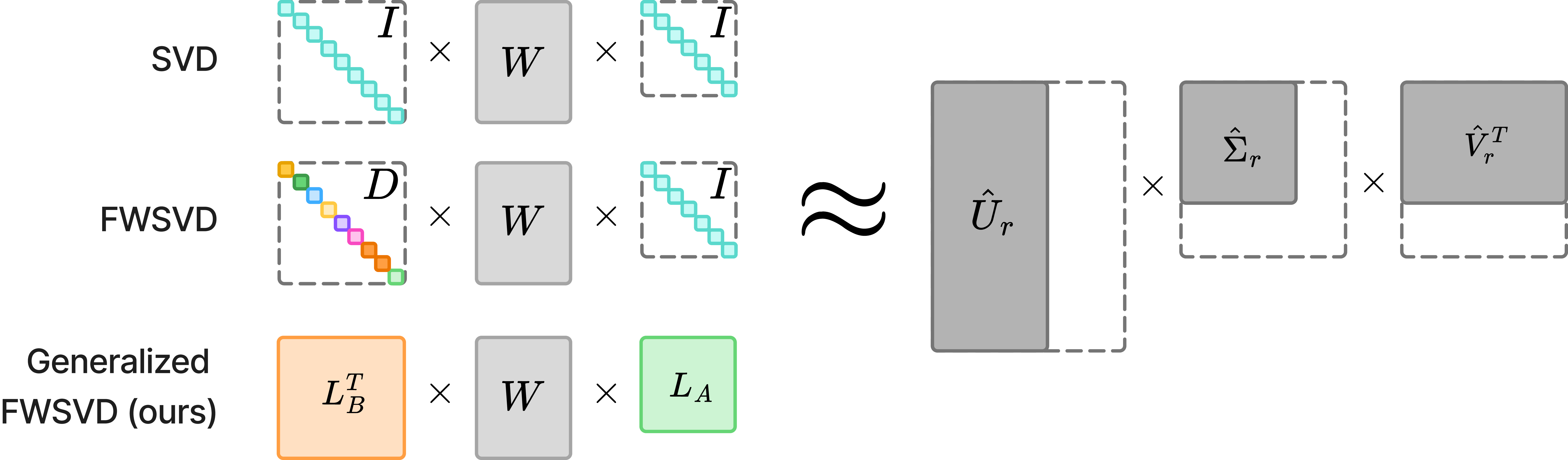
We show that FWSVD, presented in [6], is a special case of our generalized framework. The full justification is given in Appendix 9. In FWSVD, the objective minimizes a weighted reconstruction error using a diagonal matrix \(\mathbf{D}\) derived from a row-wise sum of the Fisher Information. We show that this setup corresponds to a diagonal Kronecker-factored approximation of the FIM, where \(\mathbf{D}\) arises naturally from minimizing the Kronecker approximation error. The resulting solution for the low-rank factors \(\mathbf{W}_2, \mathbf{W}_1\) matches that of FWSVD (up to a constant), which shows that their method is a special case of our more general framework.
The connection between our generalized approach, the classical SVD and FWSVD is depicted in Figure 1. Weighted SVD approaches can be interpreted as transforming the decomposed object—here, the weight matrix—into a new space where the low-rank approximation better aligns with the target task. In this formulation, the sensitivity matrices serve as transformation matrices that reweight the importance of different directions. Under this view, vanilla SVD corresponds to using identity transformations; FWSVD applies a diagonal (but non-identity) transformation on one side while keeping the other side as identity. In contrast, our method employs full, non-diagonal transformations on both sides, capturing richer structure in the parameter space.
4 Kronecker Factorization Algorithm via Rank-1 SVD↩︎
Suppose that we have a linear layer of a network with a weight matrix \(\mathbf{W}\) and define \(\mathbf{G}_i\in \mathbb{R}^{n \times m}\) as a weight gradients \(\mathcal{L}(\theta)|_{\theta= \mathbf{W}}\) on the \(i\)-th batch, and \(g_i = \mathop{\mathrm{vec}}({\mathbf{G}_i}) \in \mathbb{R}^{n \cdot m}\) - its flattening version. Then, Fisher Information \(\mathcal{I}_F(\theta)\) can be defined as an empirical mean over all batches in a dataset \(D\): \[\mathcal{I}_F(\theta^{\star}) = \mathbb{E}\left[g g^\top\right] = \frac{1}{|D|}\sum_{i=1}^{|D|}{g}_{i}^{}{g}_{i}^\top. \label{eq:J}\tag{7}\]
Kronecker product approximation is obtained by solving minimization problem: \[\min \left\| \mathcal{I}_F - \mathbf{A} \otimes \mathbf{B} \right\|_{\operatorname{F}} \label{eq:min95probles}\tag{8}\]
Kronecker product decomposition of \(\mathcal{I}_F\) is computed from a rank-1 approximation of permuted matrix \(\tilde{\mathcal{I}}_F = \mathcal{R} \mathcal{I}_F \in \mathbb{R}^{m^2\times n^2}\), as it is described in [22]. The pseudocode of the method is in Algorithm 2.

4.1 Efficient Rank-1 Computation↩︎
The primary computational bottleneck of Algorithm arises in performing SVD on the matrix \(\mathcal{\tilde{I}}_F\).
Standard SVD is computationally intractable for large matrices, so we employ truncated SVD using the Lanczos [23] method, which avoids explicit matrix construction and requires only the ability to multiply the matrix with a vector from the left or right. Even in this setting, aggregating the full second-moment gradient information across all batch samples is computationally expensive.
We can show (see Appendix 10) that permuted \(\mathcal{I}_F\) for \(i\)-th batch can be defined as the Kronecker product of the corresponding gradient matrices:
\[\label{eq:permuted95fisher} \tilde{\mathcal{I}}_F = \frac{1}{|D|}\sum_{i=1}^{|D|} \mathbf{G}_i \otimes \mathbf{G}_i,\tag{9}\] then multiplication of this matrix \(\mathcal{\tilde{I}}_F\) to a vector \(z\) from left will be: \[\mathcal{\tilde{I}}_F z = \frac{1}{k}\left(\sum_{i=1}^{k} \mathbf{G}_i \otimes \mathbf{G}_i\right) z = \frac{1}{|D|}\left(\sum_{i=1}^{|D|} \mathbf{G}_i \otimes \mathbf{G}_i\right)\mathbf{Z} = z, \text{ where } z = \mathop{\mathrm{vec}}(\mathbf{Z}), \mathbf{Z} \in \mathbb{R}^{n\times n}\]
Using property of the Kronecker product \((\mathbf{K}\otimes \mathbf{L}) \mathop{\mathrm{vec}}\left(\mathbf{C}) = \mathop{\mathrm{vec}}(\mathbf{K^\top} \mathbf{C} \mathbf{L}\right)\) we reduce the matrix-vector multiplication to a sequence of matrix multiplications. \[\tilde{\mathcal{I}}_F z = \frac{1}{|D|}\sum_{i=1}^{|D|} \mathop{\mathrm{vec}}(\mathbf{G}_i^\top \mathbf{Z} \mathbf{G}_i) \label{eq:matvec}\tag{10}\]
The derivation for right-side multiplication is analogous (see Appendix 11). Using these operations, we can obtain an approximation of the Fisher information for layers of LLMs and batch sizes used in practice within a reasonable time.
4.2 Time Complexity of the proposed Rank-1 Computation↩︎
The time complexity of computing the truncated SVD of the matrix \(\mathbf{\tilde{J}} \in \mathbb{R}^{m^2 \times n^2}\) consists of the cost of matrix-vector multiplications and the orthogonalization step. In the standard matrix-vector multiplication case, multiplying the Fisher matrix \(\mathbf{\tilde{J}}\) by a vector has a cost of \(\boldsymbol{\mathcal{O}}\left(m^2 n^2\right)\), while orthogonalization costs \(\boldsymbol{\mathcal{O}}((m^2 + n^2) \cdot r^2)\), where \(r\) is the rank of the decomposition and can typically be neglected.
However, using the structured formulation from Eq. 10 , where left matrix-vector products are implemented via multiplications with matrices \(\mathbf{G}_i^\top \in \mathbb{R}^{m \times n}\), \(\mathbf{Z} \in \mathbb{R}^{n \times n}\), and \(\mathbf{G}_i \in \mathbb{R}^{n \times m}\), the overall complexity is reduced to \(\boldsymbol{\mathcal{O}}\left(m n^2 + m^2 n\right)\). Applying analogous reasoning to the right matrix-vector products (see Eq. 15 ) one can yield the same complexity.
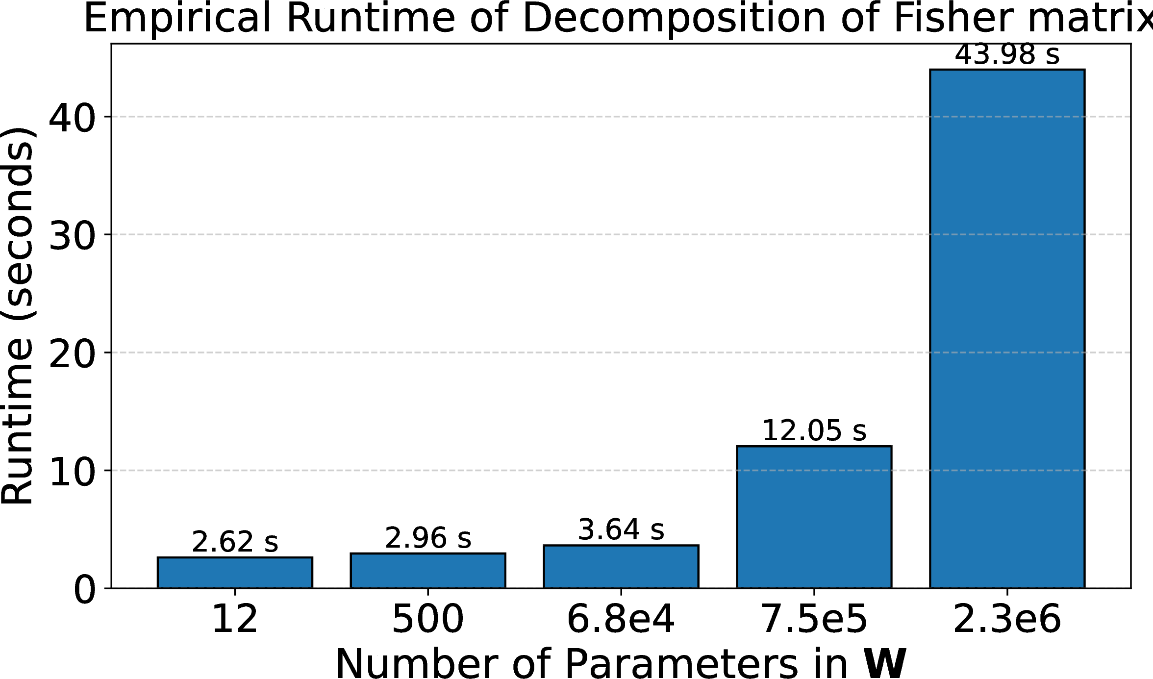
Although the proposed method exhibits cubic complexity with respect to the dimensions of the linear layer’s weight matrix, its empirical runtime grows more slowly than that of the standard matrix-vector product, which scales quartically. In large language models, where \(m\) and \(n\) are typically on the order of \(10^3\), this reduction yields a practically significant speedup. Table 3 reports the empirical decomposition times for \(\mathcal{\tilde{I}}_F\), corresponding for matrices \(\mathbf{W}\) with different sizes.
5 Numerical Experiments↩︎
To validate our theoretical contributions, we conduct extensive numerical experiments on several transformer architectures: the encoder-only BERT model [24] and the decoder-only LLM LLaMA 2 [25]. Our goal is to demonstrate the practical benefits of GFWSVD in low-rank compression under fine-tuning and evaluation protocols. We conduct all experiments on a single NVIDIA A100 GPU with latest CUDA drivers using Python 3.12. The code is available on GitHub: link.
5.1 Compressing the Transformer Encoder↩︎
In our experiments, we follow the “fine-tune then compress” pipeline, similar to FWSVD [6]. We begin by fine-tuning a pre-trained checkpoint1 of the BERT-base model on a specific downstream GLUE task. Optimal fine-tuning hyperparameters (e.g., learning rate, batch size) are selected for each task using the Optuna framework [26]. During this stage, we also collect gradients to construct the FIM \(\mathcal{I}_F\) and compute its Kronecker decomposition as described in Section 4.
Using the resulting Cholesky factors \(\mathbf{L}_\mathbf{A}\) and \(\mathbf{L}_\mathbf{B}\), we uniformly compress the fully connected layers of BERT by factorizing them into two smaller layers, following the method detailed in Section 3.1. The chosen layer-wise ranks and the resulting overall compression rate of the model are summarized in Table [tbl:tab:bert95ranks]. We reproduce the ASVD method using the original authors’ code. For FWSVD, we incorporate the newly constructed FIM into the compression process.
| Rank | C.Rate | Rank | C.Rate |
|---|---|---|---|
| 1 | \(\sim 40\%\) | 100 | \(\sim 33\%\) |
| 5 | \(\sim 40\%\) | 250 | \(\sim 23\%\) |
| 10 | \(\sim 39\%\) | 500 | \(\sim 8\%\) |
| 50 | \(\sim 36\%\) | 600 | \(\sim 1\%\) |
| Method / Rank | 600 | 500 | 250 | 100 | 50 | 10 | 1 |
|---|---|---|---|---|---|---|---|
| SVD | 0.77 | 0.76 | 0.65 | 0.47 | 0.41 | 0.42 | 0.37 |
| ASVD [5] | 0.75 | 0.71 | 0.51 | 0.46 | 0.45 | 0.36 | 0.36 |
| FWSVD [6] | 0.74 | 0.74 | 0.68 | 0.56 | 0.46 | 0.43 | 0.38 |
| GFWSVD (Ours) | 0.77 | 0.77 | 0.75 | 0.66 | 0.59 | 0.53 | 0.51 |
2pt
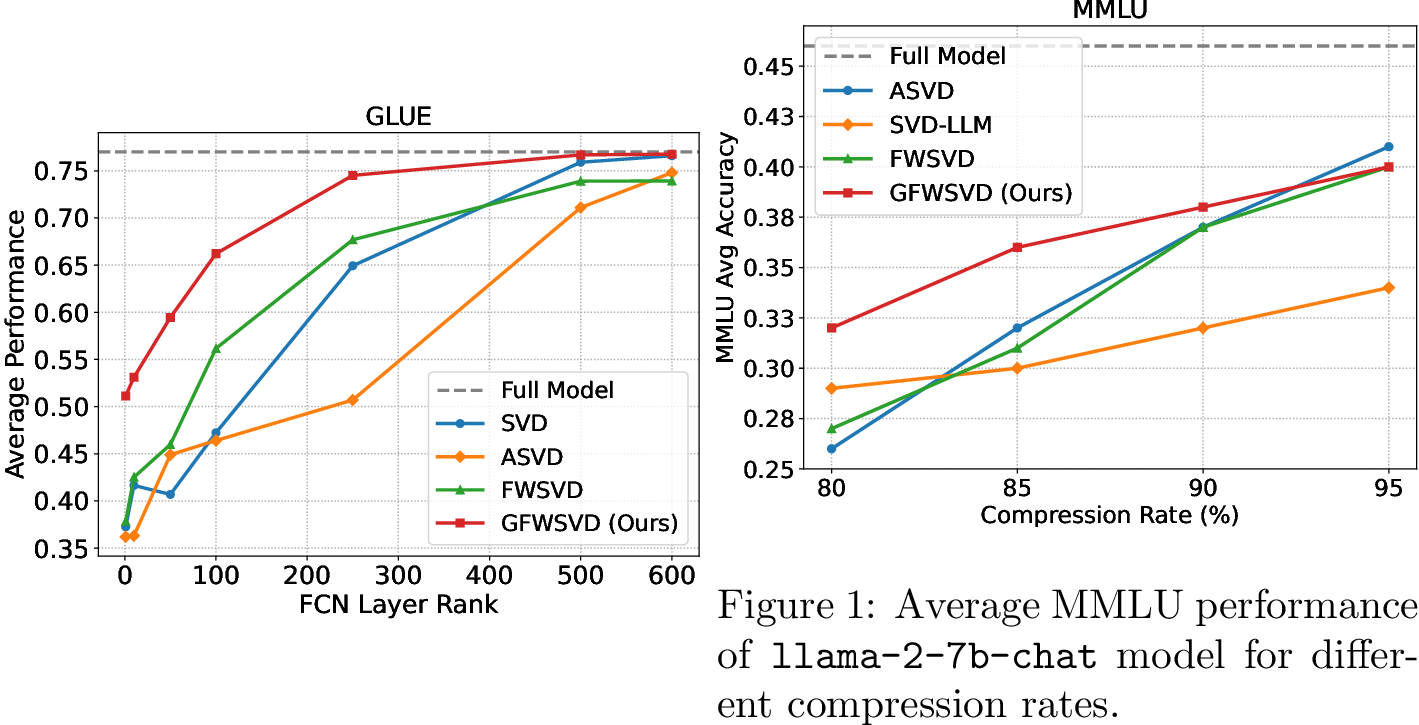
We show average compression results in Table 2 and Figure 4, extended results are in Appendix 12 in Table 4. On most of the GLUE tasks and considered compression ranks, our proposed GFWSVD approach consistently outperforms both FWSVD and SVD, with particularly strong gains at lower ranks. While ASVD exhibits relatively poor performance on several tasks (QQP, QNLI), it occasionally surpasses GFWSVD — notably on SST2 under aggressive compression.
5.2 Compressing the Transformer Decoder↩︎
We evaluate our approach on the decoder-only LLama 2 7B model2 against several competitive baselines: diagonal FI-based low-rank approximation method FWSVD [6], and two activation-based methods – ASVD [5] and SVD-LLM[7]. Notably, ASVD and SVD-LLM both rely on activation-based weighting to gauge parameter importance, while FWSVD and ours GFWSVD derive importance scores solely from gradient information.
We measure perplexity on WikiText 2 [27] and PTB [28] datasets, and 5-shot reasoning performance on the MMLU benchmark [29]. Following prior works on low-rank approximation of LLMs [5], [7], we test several compression setups, removing from 5% to 20% of original parameters.
Following standard practice in post-training LLM compression methods [5], [7], we use a randomly sampled set of sentences as calibration data to generate gradients for further obtaining the factor matrices. For calibration data, we choose the FineWeb dataset [30] due to its high quality and diversity, and collect gradients on a random subsample of size 1024. These gradients are then used to obtain \(\mathbf{L}_\mathbf{A}\) and \(\mathbf{L}_\mathbf{B}\), as well as the data needed for FWSVD. As in LLMs, uniform layer compression can disproportionately degrade performance by over-compressing critical layers and under-utilizing redundancy in less sensitive ones, so it is essential for each method to use a compression configuration that accounts for layer sensitivity. For both ASVD and SVD-LLM, we used the corresponding code released by the authors and re-ran the necessary compression pipelines for our checkpoint with all hyperparameters set to default values. For our approach, we adopted the method of per-layer importance scores as described in the ASVD work.
| Method | WikiText-2\(\downarrow\) | PTB\(\downarrow\) | Compr. | MMLU Avg\(\uparrow\) | Humanities\(\uparrow\) | Other\(\uparrow\) | Social Sciences\(\uparrow\) | STEM\(\uparrow\) |
|---|---|---|---|---|---|---|---|---|
| Full model | 6.94 | 25.75 | \(100\%\) | 0.46 \(\pm\) 0.003 | 0.43 \(\pm\) 0.01 | 0.55 \(\pm\) 0.01 | 0.53 \(\pm\) 0.01 | 0.36 \(\pm\) 0.01 |
| FWSVD [6] | 7.52 | 45.25 | \(95\%\) | 0.40 \(\pm\) 0.003 | 0.36 \(\pm\) 0.01 | 0.45 \(\pm\) 0.01 | 0.45 \(\pm\) 0.01 | 0.35 \(\pm\) 0.01 |
| ASVD [5] | 7.60 | 26.29 | 0.41 \(\pm\) 0.004 | 0.37 \(\pm\) 0.01 | 0.48 \(\pm\) 0.01 | 0.46 \(\pm\) 0.01 | 0.35 \(\pm\) 0.01 | |
| SVD-LLM [7] | 8.80 | 51.28 | 0.34 \(\pm\) 0.004 | 0.31 \(\pm\) 0.01 | 0.38 \(\pm\) 0.01 | 0.35 \(\pm\) 0.01 | 0.31 \(\pm\) 0.01 | |
| GFWSVD (Ours) | 7.16 | 28.55 | 0.40 \(\pm\) 0.003 | 0.38 \(\pm\) 0.01 | 0.47 \(\pm\) 0.01 | 0.44 \(\pm\) 0.01 | 0.33 \(\pm\) 0.01 | |
| FWSVD [6] | 11.53 | 96.62 | \(90\%\) | 0.37 \(\pm\) 0.004 | 0.34 \(\pm\) 0.01 | 0.43 \(\pm\) 0.01 | 0.42 \(\pm\) 0.01 | 0.33 \(\pm\) 0.01 |
| ASVD [5] | 8.97 | 40.12 | 0.37 \(\pm\) 0.004 | 0.33 \(\pm\) 0.01 | 0.42 \(\pm\) 0.01 | 0.40 \(\pm\) 0.01 | 0.33 \(\pm\) 0.01 | |
| SVD-LLM [7] | 9.69 | 60.82 | 0.32 \(\pm\) 0.004 | 0.30 \(\pm\) 0.01 | 0.35 \(\pm\) 0.01 | 0.32 \(\pm\) 0.01 | 0.30 \(\pm\) 0.01 | |
| GFWSVD (Ours) | 8.77 | 36.44 | 0.38 \(\pm\) 0.002 | 0.35 \(\pm\) 0.01 | 0.44 \(\pm\) 0.01 | 0.42 \(\pm\) 0.01 | 0.33 \(\pm\) 0.01 | |
| FWSVD [6] | 22.06 | 411.50 | \(85\%\) | 0.31 \(\pm\) 0.009 | 0.29 \(\pm\) 0.01 | 0.34 \(\pm\) 0.01 | 0.33 \(\pm\) 0.01 | 0.30 \(\pm\) 0.01 |
| ASVD [5] | 10.91 | 83.49 | 0.32 \(\pm\) 0.003 | 0.30 \(\pm\) 0.01 | 0.33 \(\pm\) 0.01 | 0.32 \(\pm\) 0.01 | 0.30 \(\pm\) 0.01 | |
| SVD-LLM [7] | 10.36 | 72.58 | 0.30 \(\pm\) 0.004 | 0.29 \(\pm\) 0.01 | 0.34 \(\pm\) 0.01 | 0.31 \(\pm\) 0.01 | 0.30 \(\pm\) 0.01 | |
| GFWSVD (Ours) | 10.06 | 42.19 | 0.36 \(\pm\) 0.004 | 0.33 \(\pm\) 0.01 | 0.41 \(\pm\) 0.01 | 0.38 \(\pm\) 0.01 | 0.32 \(\pm\) 0.01 | |
| FWSVD [6] | 66.37 | 1523.00 | \(80\%\) | 0.27 \(\pm\) 0.004 | 0.25 \(\pm\) 0.01 | 0.30 \(\pm\) 0.01 | 0.28 \(\pm\) 0.01 | 0.28 \(\pm\) 0.01 |
| ASVD [5] | 27.73 | 241.57 | 0.26 \(\pm\) 0.004 | 0.25 \(\pm\) 0.01 | 0.27 \(\pm\) 0.01 | 0.24 \(\pm\) 0.01 | 0.28 \(\pm\) 0.01 | |
| SVD-LLM [7] | 11.23 | 98.91 | 0.29 \(\pm\) 0.004 | 0.27 \(\pm\) 0.01 | 0.32 \(\pm\) 0.01 | 0.29 \(\pm\) 0.01 | 0.29 \(\pm\) 0.01 | |
| GFWSVD (Ours) | 11.13 | 50.50 | 0.32 \(\pm\) 0.003 | 0.30 \(\pm\) 0.01 | 0.35 \(\pm\) 0.01 | 0.34 \(\pm\) 0.01 | 0.30 \(\pm\) 0.01 |
1pt
Table 3 and Figure [fig:mmlu95avg] shows that GFWSVD consistently outperforms both simple and strong baselines across all compression rates. In particular, at the most aggressive settings (15–20% of the original parameters), our method matches or exceeds the accuracy of activation-based methods and shows substantially lower perplexities on both WikiText-2 and PTB.
6 Limitations↩︎
Our method decomposes the observed Fisher information matrix \(\mathcal{I}_F\) into a Kronecker product of two smaller matrices, \(\mathbf{Y}\) and \(\mathbf{X}\) (Eq. 8 ). While effective, this assumes exact factorization, which may not hold in practice and can limit approximation quality and task sensitivity. In LLM experiments, we also observed cases where the estimated Kronecker factors were singular, requiring regularization (e.g., \(\mathbf{Y} \leftarrow \mathbf{Y} + \alpha \operatorname{diag}{\mathbf{Y}}\)) to ensure positive definiteness and numerical stability. Although this resolves instability, it introduces additional computational overhead.
We observed that compression effectiveness varies significantly across layers, making preliminary layer selection necessary to achieve favorable trade-offs. A key limitation of our current approach is the lack of coordination across layers during compression. For effective multi – layer compression—especially in large-scale models like LLMs – it is important to account for cross-layer dependencies. Future work could focus on modeling these interactions to enable joint compression strategies.
7 Broader impacts↩︎
Our method, GFWSVD, enables more efficient compression of large language models, which can significantly reduce computational costs and energy consumption. This may help democratize access to powerful NLP tools and promote more sustainable AI deployment. However, as with any compression method, there is a risk of preserving harmful biases or weakening safety mechanisms. We advocate for responsible evaluation and deployment of compressed models, especially in sensitive applications.
8 Conclusion and Future Work↩︎
In this work we propose Generalized Fisher-Weighted SVD (GFWSVD), a gradient-based low-rank approximation method that accurately incorporates parameter importance via the full FIM. Unlike the diagonal approximation of the FIM [6], GFWSVD considers parameter correlations by leveraging a scalable Kronecker decomposition algorithm, and provides an optimal trade-off between downstream accuracy and computational efficiency. We thoroughly evaluate GFWSVD with encoder-only model BERT on GLUE benchmark and decoder only LLM LLaMa 2 on MMLU reasoning benchmark. We demonstrate GFWSVD’s superiority over diagonal Fisher- and activation-based SVD methods, particularly at extremely low ranks.
GFWSVD highlights the critical role of accurate FIM computation in compression. While our approach performs well empirically, its reliance on a rank-1 Kronecker approximation of the Fisher matrix may oversimplify important structure. Future work could explore higher-rank Kronecker series to capture richer task-relevant information, and extend the method to model cross-layer dependencies, potentially improving performance by leveraging transitive correlations across the network.
9 Appendix A: Special case of diagonal Fisher Information Matrix↩︎
In this section, we show that FWSVD, presented in [6], is a special case of our generalized approach.
In the work of [6], authors propose to minimize the following objective: \[\label{eq:fwsvd} \underset{\mathbf{W_1,W_2}}{\min} \left\| \mathbf{D}\mathbf{W}^{\star} - \mathbf{D}\mathbf{W_2}\mathbf{W_1} \right\| _F^2\tag{11}\] where \(\mathbf{D}\) is the diagonal matrix \(\sqrt {\operatorname{diag}\left(\mathbb{E} [\mathbf{G} \mathbf{G}^\top] \right)}\). Specifically, \(\mathbf{D}_{i,i} = \sqrt{\sum_{j=1}^m \mathbb{E} (\mathbf{G}_{i,j})^2 }\).
Similarly to 8 , we approximate the Fisher Information with a Kronecker product of identity matrix \(\mathbf{I}_m\) and some diagonal matrix \(\mathbf{\tilde{D}}\). As described further in Section 4 and Appendix 10, under the permutation \(\mathcal{R}\), the problem \[\label{eq:diagonal95kronecker95approx} \underset{\mathbf{D}}{\min} \left\| \mathbf{I}_F - \mathbf{I}_m \otimes \mathbf{\tilde{D}} \right\|_{\operatorname{F}}\tag{12}\] reduces to minimization of the expression \[\label{eq:diagonal95kronecker95approx95reshaped} \underset{\mathbf{d}}{\min} \left\| \mathbb{E} [\mathbf{G} \otimes \mathbf{G}] - (\mathbf{I}_n \odot \mathbf{I}_n) d \cdot \mathrm{vec} (\mathbf{I}_m)^\top \right\|_{\operatorname{F}}\tag{13}\] where \(\odot\) is a Khatri-Rao product (column-wise Kronecher product) and \(\cdot\) is a vector outer product; \(d\) is a vector diagonal of \(\mathbf{\tilde{D}}\); \(\mathbb{E} [\mathbf{G} \otimes \mathbf{G}]\) is a permuted Fisher Information matrix \(\mathbf{\tilde{I}_F}\), defined in Eq 9 .
For simplicity, we will use a shorter notation. Let \(\mathbf{E} = \mathbb{E} [\mathbf{G} \otimes \mathbf{G}]\), \(\mathbf{Z} = \mathbf{I}_n \odot \mathbf{I}_n\), \(v = \mathrm{vec} (\mathbf{I}_m)\). Then, the problem 13 is equivalent to \[\underset{\mathbf{d}}{\min} \left\| \mathbf{Z} d \cdot v^\top - \mathbf{E} \right\|_{\operatorname{F}}\] Applying first-order optimality conditions yields: \[\begin{gather} \langle \mathbf{Z} \delta d \cdot v^\top, \mathbf{Z} d \cdot v^\top - \mathbf{E} \rangle = 0 \\ \langle \delta d \cdot v^\top, \mathbf{Z}^\top \mathbf{Z} d \cdot v^\top - \mathbf{Z}^\top\mathbf{E} \rangle = 0 \\ \langle \delta d , \mathbf{Z}^\top \mathbf{Z} d \cdot v^\top v - \mathbf{Z}^\top\mathbf{E}v \rangle = 0 \\ \end{gather}\]
Since \(\mathbf{Z}^\top \mathbf{Z} = \mathbf{I}_n\), \(v^\top v = \left\| v \right\|^2_2 = \left\| \mathrm{vec}(\mathbf{I}_m) \right\|^2_2 = m\) , we have:
\[d = \frac{1}{m} (\mathbf{I}_n \odot \mathbf{I}_n)^\top \mathbb{E} [\mathbf{G} \otimes \mathbf{G}] \mathrm{vec}(\mathbf{I}_m) = \frac{1}{m} (\mathbf{I}_n \odot \mathbf{I}_n)^\top \mathrm{vec}(\mathbb{E} [G G^\top] ) = \frac{1}{m} \operatorname{diag} (\mathbb{E} [G G^\top] )\]
Thus, diagonal matrix \(\mathbf{\tilde{D}}\) from Kronecker product approximation problem 12 equals square of matrix \(\mathbf{D}\) from the FWSVD formulation 11 up to the constant \(\frac{1}{m}\).
We apply Theorem 1 to find factors \(\mathbf{W}_2\), \(\mathbf{W}_1\) for the obtained approximation \(\mathbf{I}_F = \mathbf{I}_m \otimes \mathbf{\tilde{D}}\): \[\mathbf{W}_2 = \sqrt{\mathbf{\tilde{D}}}^{-1} \mathbf{\hat{U}}_r \sqrt{\mathbf{\hat{S}}_r} = \mathbf{D}^{-1} \mathbf{\hat{U}}_r \sqrt{\mathbf{\hat{S}}_r}, \mathbf{W}_1 = \sqrt{\mathbf{\hat{S}}_r} \mathbf{\hat{V}}^\top_r\] where \(\mathbf{\hat{U}}_r \mathbf{\hat{S}}_r \mathbf{\hat{V}}^\top_r\) is r-rank SVD of \(\mathbf{\sqrt{\tilde{D}}W}^\star = \mathbf{DW}^\star\). This is the same solution that minimizes the problem 11 from FWSVD paper [6]. Consequently, FWSVD approach is a special case of diagonal Kronecker product approximation of Fisher Information.
10 Appendix B: Additional Explanations for Kronecker decomposition adaptation↩︎
Let’s show that the permuted \(\mathcal{I}_F\) in the Kronecker decomposition algorithm can be expressed as the Kronecker product of the corresponding gradient matrices.
We start with the empirical Fisher information matrix defined as:
\[\mathcal{I}_F = \frac{1}{|D|}\sum_{i=1}^{|D|}{g}_{i}^{}{g}_{i}^\top.\]
and its reordered version:
\[\label{eq:reordered95IF} \tilde{\mathcal{I}}_F = \mathcal{R} \mathcal{I}_F\tag{14}\]
Using the identity \[\operatorname{vec}(\boldsymbol{g}_i \boldsymbol{g}_i^\top) = \boldsymbol{g}_i \otimes \boldsymbol{g}_i,\] we obtain:
\[\operatorname{vec}(\mathcal{I}_F) = \frac{1}{|D|} \sum_{i=1}^{|D|} \operatorname{vec}(\boldsymbol{g}_i \boldsymbol{g}_i^\top) = \frac{1}{|D|} \sum_{i=1}^{|D|} (\boldsymbol{g}_i \otimes \boldsymbol{g}_i).\]
Let \(\mathcal{P} \in \mathbb{R}^{(ab)^2 \times (ab)^2}\) be the unique permutation matrix such that for any matrices \(\mathbf{A}, \mathbf{B} \in \mathbb{R}^{a \times b}\):
\[\mathcal{P} \cdot \operatorname{vec}(\mathbf{A} \otimes \mathbf{B}) = (\operatorname{vec}(\mathbf{A}) \otimes \operatorname{vec}(\mathbf{B})).\]
Using this definition, we can write:
\[\mathcal{P} \cdot \operatorname{vec}(\mathbf{G}_i \otimes \mathbf{G}_i) = \operatorname{vec}(\mathbf{G}_i) \otimes \operatorname{vec}(\mathbf{G}_i).\]
Therefore, the vectorized Fisher information becomes:
\[\operatorname{vec}(\mathcal{I}_F) = \frac{1}{|D|} \sum_{i=1}^{|D|} \mathcal{P} \cdot \operatorname{vec}(\mathbf{G}_i \otimes \mathbf{G}_i) = \mathcal{P} \cdot \operatorname{vec} \left( \frac{1}{|D|} \sum_{i=1}^{|D|}(\mathbf{G}_i \otimes \mathbf{G}_i) \right) = \mathcal{P} \mathop{\mathrm{vec}}(\tilde{\mathcal{I}}_F) .\]
So, \(\tilde{\mathcal{I}}_F\) can be defined as \(\frac{1}{|D|} \sum_{i=1}^{|D|}(\mathbf{G}_i \otimes \mathbf{G}_i)\). This fact is used in the accelerated adaptation of the Kronecker Factorization algorithm.
Now, suppose a \(\mathcal{I}_F\) and \(\tilde{\mathcal{I}}_F\) are connected with \(\mathcal{R} \in \mathbb{R}^{n \times n}\) (see Eq. 14 ):
\[\operatorname{vec}(\widetilde{\mathcal{I}}_F) = (I \otimes \mathcal{R}) \cdot \operatorname{vec}(\mathcal{I}_F), \mathcal{P} = I \otimes \mathcal{R}\]
11 Appendix C: Right vector-matrix multiplication↩︎
We can define right vector-matrix multiplication as follows: \[\mathcal{I}_F^\top z = (\sum_{i=1}^{|D|} \mathbf{G}_i \otimes \mathbf{G}_i)^\top z\]
Using property of the Kronecker product \((\mathbf{K}\otimes \mathbf{L}) \mathop{\mathrm{vec}}(\mathbf{C}) = \mathop{\mathrm{vec}}(\mathbf{K^\top} \mathbf{C} \mathbf{L})\): \[\label{eq:rmatvec} \mathcal{I}_F^\top z = \sum_{i=1}^{|D|} \mathop{\mathrm{vec}}(\mathbf{G}_i \mathbf{Z} \mathbf{G}_i^\top) \text{, where } z = \mathop{\mathrm{vec}}(\mathbf{Z}), \mathbf{Z} \in \mathbb{R}^{m\times m}\tag{15}\]
12 Appendix D: Extended GLUE results↩︎
We report extended compression results on tasks of GLUE benchmark in Table 4.
| Method / Dataset | MRPC\(\uparrow\) | STSB\(\uparrow\) | QQP\(\uparrow\) | MNLI\(\uparrow\) | QNLI\(\uparrow\) | RTE\(\uparrow\) | COLA\(\downarrow\) | SST2\(\uparrow\) | |
|---|---|---|---|---|---|---|---|---|---|
| Full model | 0.77 | 0.87 | 0.90 | 0.83 | 0.90 | 0.56 | 0.41 | 0.91 | |
| Compression Rate \(99\%\) (\(r=600\)) | |||||||||
| SVD | 0.67 | 0.84 | 0.90 | 0.67 | 0.90 | 0.56 | 0.58 | 0.91 | |
| ASVD [5] | 0.72 | 0.73 | 0.89 | 0.83 | 0.90 | 0.56 | 0.41 | 0.91 | |
| FWSVD [6] | 0.72 | 0.87 | 0.90 | 0.72 | 0.90 | 0.55 | 0.36 | 0.91 | |
| GFWSVD (Ours) | 0.73 | 0.87 | 0.90 | 0.73 | 0.90 | 0.56 | 0.55 | 0.92 | |
| Compression Rate \(92\%\) (\(r=500\)) | |||||||||
| SVD | 0.53 | 0.82 | 0.89 | 0.53 | 0.90 | 0.54 | 0.53 | 0.89 | |
| ASVD [5] | 0.71 | 0.56 | 0.86 | 0.81 | 0.89 | 0.53 | 0.44 | 0.88 | |
| FWSVD [6] | 0.71 | 0.87 | 0.90 | 0.71 | 0.89 | 0.56 | 0.34 | 0.91 | |
| GFWSVD (Ours) | 0.73 | 0.87 | 0.90 | 0.73 | 0.90 | 0.56 | 0.49 | 0.92 | |
| Compression Rate \(77\%\) (\(r=250\)) | |||||||||
| SVD | 0.49 | 0.68 | 0.81 | 0.49 | 0.85 | 0.50 | 0.17 | 0.57 | |
| ASVD [5] | 0.69 | 0.08 | 0.76 | 0.50 | 0.58 | 0.47 | 0.11 | 0.75 | |
| FWSVD [6] | 0.69 | 0.86 | 0.89 | 0.69 | 0.89 | 0.61 | 0.23 | 0.80 | |
| GFWSVD (Ours) | 0.71 | 0.86 | 0.89 | 0.71 | 0.89 | 0.61 | 0.38 | 0.88 | |
| Compression Rate \(67\%\) (\(r=100\)) | |||||||||
| SVD | 0.32 | 0.08 | 0.64 | 0.32 | 0.80 | 0.51 | 0.01 | 0.49 | |
| ASVD [5] | 0.58 | 0.07 | 0.74 | 0.39 | 0.50 | 0.47 | 0.05 | 0.82 | |
| FWSVD [6] | 0.69 | 0.58 | 0.87 | 0.71 | 0.86 | 0.55 | 0.21 | 0.72 | |
| GFWSVD (Ours) | 0.71 | 0.70 | 0.87 | 0.71 | 0.86 | 0.55 | 0.21 | 0.72 | |
| Compression Rate \(64\%\) (\(r=50\)) | |||||||||
| SVD | 0.32 | 0.19 | 0.57 | 0.32 | 0.78 | 0.48 | 0.02 | 0.49 | |
| ASVD [5] | 0.68 | -0.03 | 0.73 | 0.49 | 0.76 | 0.51 | -0.03 | 0.80 | |
| FWSVD [6] | 0.69 | 0.65 | 0.84 | 0.69 | 0.72 | 0.46 | 0.03 | 0.77 | |
| GFWSVD (Ours) | 0.69 | 0.65 | 0.84 | 0.69 | 0.72 | 0.46 | 0.05 | 0.77 | |
| Compression Rate \(61\%\) (\(r=10\)) | |||||||||
| SVD | 0.32 | 0.32 | 0.67 | 0.32 | 0.61 | 0.51 | 0.00 | 0.49 | |
| ASVD [5] | 0.61 | -0.14 | 0.64 | 0.40 | 0.57 | 0.49 | -0.04 | 0.76 | |
| FWSVD [6] | 0.37 | 0.32 | 0.79 | 0.37 | 0.57 | 0.49 | 0.00 | 0.49 | |
| GFWSVD (Ours) | 0.53 | 0.60 | 0.79 | 0.53 | 0.62 | 0.47 | 0.05 | 0.65 | |
| Compression Rate \(60\%\) (\(r=1\)) | |||||||||
| SVD | 0.32 | 0.04 | 0.69 | 0.31 | 0.55 | 0.53 | 0.00 | 0.49 | |
| ASVD [5] | 0.62 | -0.10 | 0.64 | 0.42 | 0.50 | 0.49 | -0.03 | 0.70 | |
| FWSVD [6] | 0.32 | 0.18 | 0.72 | 0.32 | 0.51 | 0.50 | 0.00 | 0.49 | |
| GFWSVD (Ours) | 0.42 | 0.70 | 0.74 | 0.42 | 0.65 | 0.52 | 0.05 | 0.49 | |