Keywords: oracle; information dominance; experiments; common knowledge component, information loops.

1 Introduction↩︎

Public information in strategic environments does more than reveal facts: it changes how privately informed agents reason about one another. As a result, forecasts, ratings, disclosures, and recommendations may alter equilibrium behavior even when the intermediary itself has only partial information. This raises a fundamental comparative question: when is one information intermediary more informative than another? The question is central to environments involving rating agencies, media outlets, central banks, prediction markets, and online platforms, all of which shape strategic behavior by selectively revealing information to heterogeneously informed agents.

This paper examines incomplete-information games where players are partially informed, both privately and publicly, about the realized state. The private information is provided to every player by their specific partition, and the public information is disclosed by an external source, namely, an oracle.

Formally, an oracle holds a partition of the state space and communicates through a signaling function that is measurable with respect to the oracle’s partition. Any such signaling scheme is a Blackwell experiment (see [1]), so an oracle can be viewed as a generator of experiments compatible with its information. Each experiment, combined with the players’ private partitions, induces a “guided game" with its own set of equilibria. Notably, the oracle need not know what is common knowledge among the players.

The primary objective is to compare two oracles in terms of their ability to induce equilibria across all games. Oracle 1 is said to dominate Oracle 2 if, for every game and every experiment available to Oracle 2, Oracle 1 can generate an experiment that induces exactly the same set of equilibrium distributions over state-action profile pairs.

Throughout the paper, we keep the players’ private information fixed and vary only the oracles’ signaling strategies; we also adopt a stringent notion of dominance of matching the set of equilibrium outcome distributions induced by the other oracle. This makes the comparison independent of any equilibrium-selection rule or objective the oracle might pursue, and contrasts with alternative notions that require the comparison to hold for every configuration of the players’ private information. Further discussion of these modeling assumptions and the challenges they create is given in Section 3.

Dominance has two complementary components: a local component and a global one. The local part is governed by the players’ common knowledge components (CKCs), the minimal commonly known events (see [2]). The global part is governed by a new structure, referred to as information loops: closed paths that link different CKCs through atoms of the oracle’s partition. Figure 1 illustrates an \(F_i\)-loop, induced by the partition \(F_i\) of Oracle \(i\), and consisting of three ordered pairs \(((\omega_1, \overline{\omega}_1), (\omega_2, \overline{\omega}_2), (\omega_3, \overline{\omega}_3))\). The presence of two distinct states in every CKC throughout the loop is fundamental: information transmission relies on controlling likelihood ratios across such pairs, and the loops are defined precisely because they constrain this ability.

Information loops capture a layer of structure beyond common knowledge. They arise only through interactions with an external agent who is not part of the common-knowledge structure, and they determine whether the local mimicking constructions inside each CKC can be glued into a single oracle-measurable experiment. As a consequence, refinement of partitions within every CKC is not sufficient for dominance: the more informative oracle may still face global compatibility constraints, namely, trade-offs in information transmission across CKCs.

Our analysis begins with the study of loop geometry. We identify several essential properties of information loops, the central one being the existence of an order-preserving cover. An \(F_1\)-loop admits an order-preserving \(F_2\)-cover if its pairs, excluding those that \(F_2\) does not distinguish, can be partitioned into \(F_2\)-sub-loops, each preserving the cyclic order inherited from the original \(F_1\)-loop. This property, along with several others studied in Section 4, underlies our two main results.

The first main result, Theorem 1, characterizes equivalent oracles, defined through mutual dominance. The equivalence problem is the cleanest benchmark: mutual dominance forces both oracles to agree locally within every CKC and globally on their loop structure. Specifically, Oracles 1 and 2, with partitions \(F_1\) and \(F_2\) respectively, are equivalent if and only if \(F_1\) and \(F_2\) refine each other within every CKC and every \(F_i\)-loop admits an order-preserving \(F_{-i}\)-cover, for \(i=1,2\).

We then turn to one-sided dominance, Theorem 2, our second main result and a loop-cover theorem. If Oracle 1 dominates Oracle 2, then \(F_1\) refines \(F_2\) inside every CKC, every \(F_1\)-loop is covered by \(F_2\)-loops, and whenever the cover is unique it must preserve the cyclic order of the original loop. Conversely, if \(F_1\) refines \(F_2\) inside every CKC, every \(F_1\)-loop has an order-preserving \(F_2\)-cover, and the \(F_1\)-loops are separated, then Oracle 1 dominates Oracle 2. Thus, dominance is governed by local refinement together with global loop compatibility.

These results immediately yield several benchmark cases. If the state space consists of a single CKC, or if there are no \(F_1\)-loops at all, the global loop condition is vacuous and dominance collapses to refinement within every CKC (Corollary 1).

Finally, we focus on deterministic experiments. A deterministic experiment assigns a signal to each atom of the oracle’s partition, and in this restricted setting dominance collapses to a jointly more informative (JMI) condition: Oracle 1 dominates Oracle 2 if and only if, for every deterministic experiment of Oracle 2, Oracle 1 can match the players’ joint posterior beliefs once their private information is taken into account (Proposition 3). The refinement condition in the stochastic results does not follow from the deterministic JMI criterion (Example 1), so the stochastic theory is not simply a stochastic recasting of the deterministic one.

1.1 Motivation and applications↩︎

Although Section 2 develops a complete motivating example, it is useful to discuss how our model applies more broadly, starting from the opening example in [3]. Recall that a fully informed prosecutor seeks to persuade an uninformed judge to convict a defendant. To achieve this, the prosecutor commits to a signaling structure designed to induce conviction with some probability.

Taking this example a step further, in many judicial systems the prosecutor must persuade not only a judge but also a jury.⁵ Moreover, the prosecutor is typically not fully informed, while neither the judge nor the jury is completely uninformed. Each holds personal intuitions, prior beliefs, and subjective perspectives. In practice, the prosecutor faces informational constraints analogous to those encountered by the oracle in our framework. In this analogy, the prosecutor is the oracle, the judge and jury are the players, and their private intuitions and priors correspond to the players’ private information. Our partial order ranks prosecutorial information systems (e.g., evidence-disclosure regimes) by the sets of equilibrium verdicts they can induce across all such games. The same logic applies to the problem of belief polarization in our Section 2 example: different “oracles" (fact checkers) can be ranked by the equilibrium depolarization patterns they can implement.

This perspective highlights why the partial ordering of oracles is a central comparative notion in such environments: standard tools (e.g., concavification) may fail under partial and asymmetric information. In a similar set-up, [4] show that the feasible set of joint posterior beliefs is typically non-convex given a non-binary state space, when both the oracle and the players possess private and partial information. Consequently, a partial ordering of “experiment generators’’ becomes a powerful methodological tool for analyzing these problems. Practically, this means that in settings with partially informed judges/juries or central banks/markets, one can compare alternative information systems (transparency regimes, disclosure formats, types of forecasts) by asking which oracle dominates another, without solving a fully-fledged information‑design problem.

1.2 Relation to literature↩︎

[1], [5] provides the classic comparison of experiments for a single decision maker: one information structure dominates another if it yields weakly higher expected utility in every decision problem. We extend this framework along two dimensions. First, we move from decision problems to incomplete‑information games, where the objects being compared are equilibria of “guided games" induced by an oracle’s signals. Second, instead of a fixed experiment, an oracle is a generator of experiments compatible with its partition. Our dominance notion is therefore about the ability of one oracle to replicate the equilibrium outcome distributions that another oracle can induce, rather than optimizing a particular decision maker’s payoff.

[6] strengthen Blackwell by requiring robustness to arbitrary auxiliary signals and decision problems and characterize strong Blackwell dominance between two signals. Their analysis compares two information sources (signals) that are robust to any external information source and decision problem. In contrast, we fix the players’ private information structures and the prior, and compare oracles that can implement any experiment measurable with respect to their partitions. Our dominance relation is specific to a given configuration of players’ information and to strategic interaction, not to a universal set of decision problems.

A related literature compares information structures in games and establishes partial orders. [7] analyzed zero-sum games, offering an analogous result to Blackwell’s by characterizing when one information structure is more advantageous for the maximizer. [8], [9] analyze signaling and mediation in common‑interest games and show how variants of Blackwell garbling characterize outcome equivalence. Likewise, [10] characterize dominance among two information structures through the concept of individual sufficiency, an extension of Blackwell’s notion of garbling to \(n\)-player games. A common feature of these papers is that they compare fixed information structures (typically private signals) and use versions of Blackwell’s garbling to capture dominance. We instead hold players’ private information fixed and compare oracles that provide public signals, subject to an oracle-measurability constraint (the oracle cannot condition on players’ private signals). For this reason, oracle dominance is not meant to coincide with, or simply specialize, [10] to public signals: even under a “public-signal-only” restriction, their order is a pairwise comparison of two fixed information structures, whereas our is a comparison over the menus of feasible public experiments generated by different oracle partitions. Dominance in our setting is driven by the implementable joint posterior beliefs, constrained by CKCs and information loops.

Another strand studies mediators in incomplete‑information games who correlate players’ actions through private recommendations, often without adding information about the realized state; see [11] and [12] among others. In these models, the mediator’s role is to coordinate actions so as to implement correlated equilibria. Our oracles differ in two respects: they provide public signals rather than private recommendations, and their role is not to coordinate actions but to change beliefs. As a result, dominance in our setting cannot be reduced to the richness of the correlated‑equilibrium correspondence.

Our departure from existing dominance notions (see, e.g., [12] and [10]) lies in restricting information provision to public disclosure, given players’ private information and the Oracle’s information. This restriction imposes global measurability and consistency constraints that are absent in other frameworks. If players’ private information is trivial, if the Oracle is allowed to issue private recommendations, or if the Oracle is agnostic about players’ information and the comparison ranges over all possible information structures, these measurability constraints vanish, and our notion of dominance collapses to standard refinement or Blackwell-type comparisons. The conceptual contribution of this paper is to isolate and clarify the role of public disclosure in shaping the interaction between fixed players’ private information and the Oracle’s information, and to show how this interaction fundamentally alters the set of attainable equilibrium outcomes.

Our use of common knowledge components is rooted in the epistemic foundations of games. [2] defines common knowledge and the induced partition into common knowledge components. [13], [14], and [15] clarify how hierarchies of beliefs and type spaces encode such information. Our model builds on these studies by fixing the partition structures while varying only the oracle’s public experiment. The novel constraints we study arise from global measurability across CKCs (via loops), not from additional complexity in private belief hierarchies. Information loops then formalize how public measurability links different CKCs and constrains the set of posterior profiles that an oracle can generate.

The dominance problem, and in particular the analysis of order-preserving covers, can be partially translated into the study of Eulerian directed multigraphs. We employ the main results and techniques of [16] to show that the unique-cover condition corresponds to the case in which distinct loops intersect in at most one atom. To the best of our knowledge, however, no general theory currently exists for the order-preservation property.

1.3 The structure of the paper↩︎

The paper is organized as follows. In Section 2, we provide a simple example to illustrate the key concepts of the paper. Section 3 presents the model, the dominance relation, and the posterior-mimicry perspective used throughout the analysis. Section 4 introduces common knowledge components, local refinement, information loops, covers, and order preservation. Section 5 gives the complete characterization of equivalent oracles. Section 6 studies one-sided stochastic dominance and states the loop-cover dominance theorem. Section 7 collects the benchmark cases: unique CKC, acyclic/no-loop stochastic structures, non-informative loops, the two-CKC case, and deterministic dominance. Section 8 concludes.

2 Fact checking and belief depolarization: an example↩︎

The problem of polarization, whether affective, ideological, or identity-driven, has received substantial attention in both public discourse and academic research (e.g., [17]; [18], and [19]). Technological progress has not mitigated this problem. Selective exposure to information and the ease of coordinated disinformation may instead amplify disagreement, making fact checking and depolarization particularly challenging. The following stylized example illustrates how our framework captures these forces.

Consider two individuals (or populations) who receive information from different sources about an unknown state \(\omega\in\Omega=\{\omega_1,\omega_2,\omega_3,\omega_4\}\) with common prior \(\mu=(\tfrac{1}{16},\tfrac{4}{16},\tfrac{5}{16},\tfrac{6}{16})\). Their private information is represented by the partitions \(\Pi_1=\{\{\omega_1,\omega_3,\omega_4\},\{\omega_2\}\}\) and \(\Pi_2=\{\{\omega_1\},\{\omega_2,\omega_3,\omega_4\}\}\). To abstract from actions and payoffs, polarization is measured by the expected \(\ell^1\)-disagreement \(D(\tau)=\mathbb{E}[\|\mu^1_{\tau}-\mu^2_{\tau}\|_1]\), where \(\mu^i_{\tau}\) denotes player \(i\)’s posterior given her private information and the public signal generated by \(\tau\).⁶ If no public information is provided, that is, if the public signal is constant, each player conditions only on her private information. A direct computation yields \(D(\tau^{\mathrm{Const}})=\tfrac{407}{480}\approx0.848\).

Now consider a fact checker, referred to as Oracle \(1\), who seeks to reduce disagreement. Oracle \(1\) observes the public partition \(F_1=\{\{\omega_1,\omega_3\},\{\omega_2,\omega_4\}\}\). While a perfectly informed oracle could eliminate disagreement, in practice verifiable evidence is often limited. In this example, \(F_1\) represents the informational constraint faced by the fact checker. If Oracle \(1\) fully reveals the realized \(F_1\)-cell, then \(D(\tau_1^{\mathrm{Full}}) = \tfrac{97}{120}\approx0.808\), so revealing \(F_1\) reduces disagreement relative to having no oracle.

Next, define an \(F_1\)-measurable experiment with two public signals \(s_1,s_2\) by \[\tau_1^{\mathrm{Noisy}}(s_1\mid \omega)= \begin{cases} 0, & \text{if } \omega\in\{\omega_1,\omega_3\},\\[2pt] \tfrac{3}{4}, & \text{if } \omega\in\{\omega_2,\omega_4\}, \end{cases} \qquad \tau_1^{\mathrm{Noisy}}(s_2\mid \omega)=1-\tau_1^{\mathrm{Noisy}}(s_1\mid \omega).\] This \(F_1\)-measurable experiment is a garbling of \(\tau_1^{\mathrm{Full}}\) and hence Blackwell-inferior to full revelation of \(F_1\).⁷ Nevertheless, a direct computation gives \(D(\tau_1^{\mathrm{Noisy}})=\tfrac{31}{40}=0.775<D(\tau_1^{\mathrm{Full}})\), so full revelation is strictly dominated for the purpose of minimizing expected disagreement.

Consider instead Oracle \(2\), endowed with the public partition \(F_2=\{\{\omega_1,\omega_2\},\{\omega_3,\omega_4\}\}\). Notice that \(F_2\) neither refines \(F_1\) nor is refined by it, so neither oracle Blackwell-dominates the other. If Oracle \(2\) fully reveals the realized \(F_2\)-cell, then for every \(\omega\in\Omega\), we get \(\Pi_1(\omega)\cap F_2(\omega)=\Pi_2(\omega)\cap F_2(\omega)\). Thus the players condition on the same event at every state and therefore hold identical posterior beliefs, implying \(D(\tau_2^{\mathrm{Full}})=0\). In summary, \[D(\tau^{\mathrm{Const}})>D(\tau_1^{\mathrm{Full}})>D(\tau_1^{\mathrm{Noisy}})>D(\tau_2^{\mathrm{Full}})=0.\]

This example highlights several themes that recur throughout our analysis. First, players’ private information substantially complicates the analysis, and the problem of polarization more generally, to the extent that even garbling need not be “inferior" to full revelation. Second, the oracle’s objective in this example, and more generally in any strategic environment we consider, is to control the distribution of joint posterior beliefs, which encodes the entire hierarchy of beliefs. This objective is distinct from, and typically more restrictive than, coordination via correlated equilibrium in the sense of [11]. Third, this example also motivates the general question: given players’ partitions (possibly with multiple CKCs), when does Oracle 1 dominate Oracle 2 in the sense that for every experiment \(\tau_2\) there exists an experiment \(\tau_1\) inducing the same joint distribution of posterior beliefs (same polarization)?

3 The model and posterior mimicry↩︎

A guided game comprises a Bayesian game and an oracle. The oracle’s role is to provide information that enables a different, and preferably broader, range of equilibria. It does so through public signaling, and our analysis seeks to characterize the extent to which oracles can expand the set of equilibrium payoffs.

We begin by defining the underlying Bayesian game. Let \(N = \{1, 2, \dots, n\}\) be a finite set of \(n \geq 2\) players, and let \(\Omega\) denote a non-empty, finite state space. Each player \(i \in N\) has a non-empty set of actions \(A_i\) and a partition \(\Pi_i\) over \(\Omega\), representing the information available to player \(i\). Denote the set of action profiles by \(A = \times_{i \in N} A_i\). The utility function for each player \(i \in N\) is \(u_i: \Omega \times A \to \mathbb{R}\), which maps states and action profiles to real-valued payoffs.⁸

To extend the basic game into a guided game, we introduce an oracle who provides public information before players choose their actions. The oracle is endowed with a partition \(F\) of the state space \(\Omega\), and a countable set \(S\) of possible signals. A signaling strategy of the oracle is an \(F\)-measurable experiment \(\tau : \Omega \to \Delta(S)\), where \(\Delta(S)\) is the set of probability distributions on \(S\) with finite support. We denote by \(\tau(s|\omega)\) the probability that the oracle sends signal \(s\) when the realized state is \(\omega\).

The guided game evolves as follows. First, the oracle publicly announces an experiment \(\tau\). Then, a state \(\omega \in \Omega\) is drawn according to a common prior \(\mu \in \Delta (\Omega)\) with full support. Each player \(i\) is privately informed of \(\Pi_i(\omega)\), which is a set of states containing \(\omega\) and also an atom of player \(i\)’s private partition. Finally, a signal \(s\in S\) is drawn according to \(\tau(\omega)\) and is publicly announced.

Let the join⁹ \(\Pi_i \vee F'\) denote the updated information (i.e., partition) of player \(i\) given \(\Pi_i\) and some partition \(F'\). Let \(\mu^i_{\tau|{\omega},s} = \mu(\cdot|\Pi_i({\omega}),\tau,s) \in \Delta(\Omega)\) denote player \(i\)’s posterior belief after observing \(\Pi_i(\omega)\) and a realized signal \(s\) according to \(\tau(\omega)\), and let \(\mu_{\tau,s} = \bigl\{ (\mu^i_{\tau|{\omega},s})_{i\in N}:\omega\in\Omega \; { \rm s.t.} \;\tau(s|\omega)>0 \bigr\}\) be the set of joint posteriors associated with \(\tau\) and a signal \(s\), across all relevant states. The joint posteriors capture each player’s belief about the realized state and their beliefs about others’ beliefs, as well as higher-order beliefs. We use \(\mu_{\tau}\) to denote the distribution over all joint posteriors induced by \(\tau\) across all signals, and use \({\rm Post}(\tau) = {\rm Supp}(\mu_{\tau})\) to denote its support. Thus, every experiment \(\tau\) yields an incomplete-information game \(G(\tau) = (N,(A_i)_{i\in N},\mu_{\tau}, (u_i)_{i\in N})\). When there is no risk of ambiguity, we denote the incomplete-information game without \(\tau\) by \(G\).

3.1 Partial ordering of oracles↩︎

To discuss the role of the oracle in the current framework, we define a relevant solution concept, referred to as a Guided equilibrium, which incorporates the oracle’s strategy. Formally, let \(\sigma_i: \Pi_i\times S\rightarrow \Delta (A_i)\) be a strategy of player \(i\). A tuple \((\tau,\sigma_1,\dots,\sigma_n)\) is a Guided equilibrium if \((\sigma_1,\dots,\sigma_n)\) is a Nash equilibrium in the incomplete-information game \(G(\tau)\).

The notion of a Guided equilibrium defines a partial ordering of oracles, i.e., a partial relation over their partitions according to the sets of equilibria. To define this relation, let \(\rm{NED}(G(\tau)) \subseteq \Delta(\Omega \times A)\) be the set of distributions over \(\Omega \times A\) induced by Nash equilibria given \(G\) and \(\tau\).¹⁰ Now consider two oracles, Oracle \(1\) and Oracle \(2\), and denote the generic partition and experiment of Oracle \(j\) by \(F_j\) and \(\tau_j\), respectively.

Intuitively, Oracle 1 dominates Oracle 2 if, whatever experiment Oracle 2 uses and whatever game is played, Oracle 1 can choose an experiment that yields exactly the same set of equilibrium outcome distributions. Note that a direct comparison of the games’ equilibria is problematic because the players’ strategies depend on the oracles’ experiments.

Three points are worth noting here. First, one could consider defining dominance between oracles in a more robust manner by allowing players’ information structures to vary over a set of possible partitions. If dominance were required to hold uniformly over all such partitions, the comparison problem would become rather simple. In particular, the set of admissible information structures would include the case of trivial private information. In that case, the common-knowledge structure admits no loops and, by our results, oracle dominance reduces to partition refinement. The substantive challenge in our framework arises precisely because players’ information partitions are fixed and predetermined, so that dominance must be assessed under binding measurability and common-knowledge constraints.

Second, Definition 1 compares oracles via equality of equilibrium distributions rather than inclusion. Analogously, one can define dominance in terms of equilibrium payoff sets, either via equality or inclusion. Outcome–based dominance implies the corresponding payoff–based notions, but the former is more natural when the objective is to control actions and aggregate outcomes, whereas payoff–based notions suit environments that focus on agents’ utilities. We adopt this stronger notion to avoid imposing a specific equilibrium-selection rule (which may diverge from the Pareto frontier), and to keep the dominance relation independent of any objective functions that might be assigned to the oracles in a parallel setup.

Third, another way to compare oracles is to treat them as strategic players in some sender–receiver game, assign payoff functions, and say that Oracle 1 is more informative than Oracle 2 if it obtains (weakly) higher equilibrium payoffs in every such game. This approach faces several difficulties: (i) equilibria are typically multiple (so oracle payoffs depend on an arbitrary selection rule); (ii) it presumes that the oracle knows the players’ private information partitions (and more generally their type structure); and (iii) it ties the comparison of information structures to particular oracle objectives. By contrast, our dominance notion compares oracles through the equilibrium outcome distributions they induce for a fixed configuration of players’ information, which is common knowledge among the players but not necessarily to the oracle. This lets us analyze the oracles’ information partitions, and the associated notions, independently of any objectives they may have.

The analysis below repeatedly uses the following posterior-mimicry perspective. For any experiment \(\tau\), the induced guided game depends on \(\tau\) only through the distribution \(\mu_{\tau}\) over joint posterior profiles. Thus, to prove that one oracle dominates another, we construct an experiment that reproduces that distribution. Conversely, when such posterior mimicry fails, proper-scoring-rule games separate the two oracles, and the induced equilibrium distributions cannot coincide in every game.¹¹ This is summarizes in the following lemma (all proofs are deferred to Appendix 9).

4 Information loops↩︎

Our characterization of dominance has two components: a local one, comparing the oracles’ partitions within each CKC, and a global one, capturing how the two partitions link different CKCs. To analyze the global component, we develop a theory of information loops, presented below.

4.1 Common knowledge components and local refinement↩︎

To define the local part of stochastic dominance, recall the notion of a common knowledge component. Following [2], an event \(E\) is a common knowledge component (CKC) of the partitions \(\Pi_1,\Pi_2, \dots, \Pi_n\) if it is an element in the meet \(\bigwedge_{i=1}^n \Pi_i\), which is the finest common coarsening of all the partitions. That is, a CKC is a minimal event (inclusion-wise) that is common knowledge among the players. Within each CKC, all posteriors and hence equilibrium payoffs are determined solely by the information available inside that component, so players’ expected payoffs and the oracle’s impact can be analyzed CKC-by-CKC.

For a partition \(F\) and a CKC \(C\), write \(F|_C\) for the restriction of \(F\) to \(C\), namely the collection of non-empty sets \(A\cap C\) with \(A\in F\). We say that \(F_1\) refines \(F_2\) in the CKC \(C\) if \(F_1|_C\) refines \(F_2|_C\), and we say that \(F_1\) refines \(F_2\) in every CKC if this condition holds for every common knowledge component. This local refinement condition is the within-component part of dominance. The remaining difficulty is global: a single \(F_1\)-measurable experiment must be chosen across all CKCs, and this creates additional measurability constraints.

When there is a single CKC, dominance is essentially local: refinement inside that component is enough to reproduce the relevant posterior distributions. With several CKCs, this local argument no longer settles the problem. Atoms of the oracle partition may connect different CKCs, and the mimicking experiment must be measurable across all these links simultaneously. The compatibility constraints generated by such cross-component links are the source of the loop restrictions below. Appendix 10.1 gives examples showing that, with several CKCs, a mimicking oracle may need to use a different signal space than the oracle it mimics, even when the two oracles have the same information inside each CKC.

4.2 Information loops and covers↩︎

We now define the loop objects that create global constraints across CKCs. Assume that \(C_1,\dots,C_l\) are mutually exclusive CKCs such that \(\Omega=\bigcup_{j=1}^l C_j\). A key aspect of our analysis is that atoms of an oracle partition may connect different CKCs. A sequence of such connections can form a closed path, which we call an information loop, or simply a loop.

To understand information loops, one can view the CKCs as the vertices of a multigraph. An edge connects two CKCs if there exist \(\omega_{j+1}\) and \(\overline{\omega}_{j}\) that belong to the same \(F_i\)-partition element (this corresponds to the second requirement). An information loop then parallels an Eulerian graph, where there is a walk that includes every edge exactly once (the last requirement in the definition) and ends back at the initial vertex (hence the requirement \(m+1\equiv 1\)). The restriction \(C_{r_j}\neq C_{r_{j+1}}\) focuses attention on the genuinely cross-CKC links, because those are the links that create global compatibility constraints. An illustrative loop is given in Figure 1 above.

The reason loops matter is immediate from measurability. If \(\tau_i\) is \(F_i\)-measurable and \((\omega_1,\overline{\omega}_1,\dots,\omega_m,\overline{\omega}_m)\) is an \(F_i\)-loop, then for every fully supported signal \(s\), \[\label{eq:32loop-product-constraint} \prod_{j=1}^m \frac{\tau_i(s\mid \omega_j)}{\tau_i(s\mid \overline{\omega}_j)}=1.\tag{1}\] Indeed, \(\overline{\omega}_j\) and \(\omega_{j+1}\) belong to the same \(F_i\)-atom, so the denominator at one step equals the numerator at the next step. Thus an \(F_1\)-loop imposes a product restriction that every \(F_1\)-measurable experiment must satisfy. The central question is when every \(F_2\)-measurable experiment that is locally mimicked (within every CKC) also respects these loop restrictions. We express the answer through the following notion of covers.

In simple terms, an \(F_{-i}\)-cover decomposes the \(F_i\)-loop into \(F_{-i}\)-loops, together with pairs for which Oracle \(-i\) cannot provide additional information. Figure 2 illustrates the definition. Panel (a) shows an \(F_1\)-loop (consisting of \((({\omega}_j,\overline{{\omega}}_j))_{j=1,\dots,4}\)) covered by two order-preserving \(F_2\)-loops. Panel (b) shows a case in which a candidate \(F_2\)-loop does not cover the original \(F_1\)-loop, because it does not use the same ordered CKC-pairs (\(\overline{\omega}_1\) is linked to \(\overline{\omega}_3\) instead of \(\omega_3\)). Panel (c) shows a cover that is not order-preserving (the pair \((\omega_3,\overline{\omega}_3)\) appears before \((\omega_2,\overline{\omega}_2)\)). Our main dominance result (Theorem 2) states that order-preservation is necessary for dominance whenever the cover is unique, and that order-preserving covers are sufficient under separated loops.

4.3 Irreducible and informative loops↩︎

The ability to classify covers, and specifically order-preserving covers, is rather difficult. It appears that there is currently no relevant theory for this classification. To face this challenges, we decompose loops and covers into smaller objects, referred to as irreducible loops, and use these objects as building blocks in our main results. Formally, an \(F_i\)-loop is irreducible if it does not contain a smaller \(F_i\)-loop using only states from the original loop.

We also distinguish loops according to whether another oracle separates the two states that lie in the same CKC-pair. The non-informative case will be used in Corollary 2 as a sufficient condition for dominance.

If an \(F_1\)-loop is \(F_2\)-non-informative, then the loop does not pose a mimicking challenge for Oracle 1, as Oracle 2 cannot provide any relevant information in any of the pairs. Algebraically, every \(F_2\)-measurable likelihood ratio \(\tfrac{\tau_2(s\mid\omega_j)}{\tau_2(s\mid\overline{\omega}_j)}\) equals one. Thus the \(F_1\)-loop product restriction in Eq. 1 is automatically satisfied. More generally, the next proposition records the elementary loop facts that allow us to reduce the analysis to irreducible and fully informative loops.

We use Proposition 1, together with Proposition 4, which establishes additional properties of loops and is proved in Appendix 9.2, in the next two sections: first to characterize equivalent oracles, and then to establish necessary and sufficient conditions for one-sided dominance.

5 Equivalent oracles↩︎

We begin the substantive comparison of oracles with the two-sided problem, characterizing necessary and sufficient conditions for each oracle to dominate the other. Formally, Oracle \(1\) is equivalent to Oracle \(2\), written \(F_1 \sim F_2\), if \(F_i \succeq_{\mathrm{NE}} F_{-i}\) for \(i = 1, 2\).

The loop geometry developed above is sharpest in this setting. Equivalence requires that the two partitions agree within every CKC and satisfy the global loop constraints jointly generated by the two partitions. In particular, every irreducible \(F_i\)-loop must be covered by \(F_{-i}\)-loops. This condition is necessary but not sufficient: equivalence further requires that every irreducible \(F_i\)-loop with at least six states is itself an irreducible \(F_{-i}\)-loop, which implies order-preservation. (The minimum number of states in a loop is four, and every such loop is automatically order-preserving, so the six-state threshold is the first at which the condition becomes non-vacuous.) Theorem 1 provides this characterization.

The equivalence loop condition reflects a symmetry requirement on measurability: if one oracle is constrained by an information loop, the other must be constrained by a corresponding loop. The proof of the theorem leans heavily on irreducibility, through the final statement of Proposition 1: every reducible loop either intersects some CKC more than once or contains at least four states within a single partition element of \(F_i\). Under equivalence, \(F_1\) and \(F_2\) coincide within every CKC, so neither case generates an asymmetric constraint. In the first case, the loop decomposes into disjoint sub-loops, and the associated constraints apply identically on both sides. In the second case, the four states in a common \(F_i\)-atom either generate a new loop, which is then covered (with a decomposition matching that on the other oracle’s side), or fail to generate any loop at all, so no binding constraint arises.

The proof of Theorem 1 also uses a refinement of this idea. An \(F_i\)-loop is type-2 irreducible if no four of its states lie in the same partition element of \(F_i\). This condition is strictly weaker than irreducibility, since a type-2 irreducible loop may still intersect the same CKC multiple times and hence admit a decomposition into sub-loops. Even so, we show that \(F_1\) and \(F_2\) coincide along every type-2 irreducible loop.

From type-2 irreducible loops we construct the basic building blocks of the analysis, called clusters. Two type-2 irreducible loops are said to be connected if they intersect a common CKC, and the transitive closure of this relation partitions the loops into disjoint families. Each such family determines a cluster, namely, the set of CKCs collectively intersected by its loops. We prove that the oracles’ partitions agree within every cluster. Clusters therefore form the basic structure on which equivalence is established, after which the analysis extends to simpler inter-cluster connections involving only a single partition element of \(F_i\).

6 One-sided dominance↩︎

We can now state the main one-sided dominance result. The theorem has two parts: the first gives necessary conditions for dominance in general, and the second gives a sufficient condition when the \(F_1\)-loops are separated. We say that the \(F_1\)-loops are separated if no two of them share either a CKC or an \(F_1\)-atom. Together, the two parts isolate the two forces underlying dominance: local refinement within CKCs and global compatibility of loop constraints.

(i) *$F_1$ refines $F_2$ in every *CKC*;*

(ii) *every $F_1$-loop has a cover by $F_2$-loops; and*

(iii) *if an $F_1$-loop has a unique $F_2$-cover, then the cover is
      order-preserving.*

The necessity part shows that a dominant oracle must satisfy both local and global constraints. The local constraint is that \(F_1\) refines \(F_2\) within every CKC. The global constraint is that every \(F_1\)-loop is covered by \(F_2\)-loops. In particular, when an \(F_1\)-loop admits a unique cover, that cover must preserve the cyclic order, since otherwise the likelihood ratios that must be matched around the loop would become inconsistent with \(F_1\)-measurability. Building on [16] on Eulerian directed multigraphs, we show that the unique-cover condition corresponds to the case in which distinct loops intersect in at most one atom.

The sufficiency part shows that local refinement together with order-preserving covers implies dominance whenever the \(F_1\)-loops are separated. Order-preserving covers ensure consistency of the cyclic likelihood-ratio constraints along each loop, while the separation condition allows the resulting local mimicking constructions to be glued across loops. The proof also relies on a tree-mimicry argument: informative paths create no compatibility obstruction, and the only obstruction arises from closing cycles.

7 Acyclic benchmarks and deterministic experiments↩︎

The preceding sections characterize the two ingredients of oracle comparisons: local refinement within each CKC and the global loop geometry. We conclude the body of the paper with two benchmark environments in which the general constraints simplify. In unique-CKC and acyclic stochastic structures, the global ingredient is vacuous and dominance reduces to local refinement. Under deterministic signaling, the loop geometry simplifies into a joint-partition condition.

7.1 Benchmark cases↩︎

Theorem 2 turns into a full characterization in two benchmark cases: a unique CKC and no information loops. In both cases, dominance collapses to local refinement. (The proof follows directly from Theorem 2, thus omitted.)

(i) *$F_1$ refines $F_2$;*

(ii) *$F_1 \succeq_{\rm{NE}} F_2$;*

(iii) *For every $\tau_2$, there exists $\tau_1$, so that
      ${\rm Post}(\tau_1) \subseteq {\rm Post}(\tau_2)$;*

(iv) *For every $\tau_2$, there exists $\tau_1$, so that
     ${\rm Post}(\tau_1) = {\rm Post}(\tau_2)$;*

(v) *For every $\tau_2$, there exists $\tau_1$, so that
    $\mu_{\tau_1} = \mu_{\tau_2}$.*

The first part is the unique-CKC characterization. The second part is the acyclic benchmark. The proof of the acyclic benchmark constructs a graph whose vertices are CKCs and whose edges connect CKCs intersected by a common atom of \(F_1\). The no-loop assumption makes each connected component of this graph a tree. On a tree, one can assign one independent signal coordinate to each edge and then glue the local mimicking strategies without generating any cyclic compatibility condition.

Next, we record two useful special cases. The first is the case of non-informative loops, in which the loop constraints imposed by \(F_1\) are already respected by \(F_2\). The second is the two-CKC case, where the balance/cover condition is both necessary and sufficient.

The two-CKC case is especially tractable. Every loop consists of two CKC-pairs, and a cover leaves only two possibilities: either the loop is \(F_2\)-non-informative, or it is itself an \(F_2\)-loop. The first case is covered by Corollary 2; the second allows Oracle 1 to satisfy the same loop constraint as Oracle 2. In both cases, the order-preservation requirement is vacuous.

7.2 Deterministic experiments↩︎

This section focuses on dominance when oracles are restricted to deterministic experiments. Throughout the section, we consider only deterministic experiments, namely maps \(\tau_i:F_i\to S\) for each Oracle \(i\). We identify each such experiment with the partition of \(\Omega\) that it induces. Equivalently, a deterministic experiment of Oracle \(i\) is a coarsening of \(F_i\).

The characterization is based on the ability of one oracle to match the players’ joint posterior beliefs, for any given deterministic experiment of the other oracle. More formally, we say that Oracle 1 is jointly more informative (JMI) than Oracle 2 if, for every deterministic experiment of Oracle 2, there exists a deterministic experiment of Oracle 1 that induces the same posterior partition for every player.

Evidently, dominance does not require an oracle to possess information that every player has, even if that information is available to the other oracle. The same relation can also be expressed directly in terms of the oracles’ coarse partitions.

The partial order generated by the JMI notion need not coincide with the usual refinement order. For example, consider the trivial case in which the players have perfect information. Then every oracle is jointly more informative than every other oracle, independently of their partitions. Nevertheless, in Section 7.3.1, we show that, when there is a unique CKC and every oracle is JMI than the other, then their partitions coincide.

One can also bridge the gap between JMI and refinement by allowing the players’ partitions to vary.¹⁵ If JMI is required to hold for every profile of players’ partitions, then, in particular, it must hold when all players have the trivial partition. In that case, Oracle \(1\) must be able to match every deterministic experiment \(\tau_2\), so \(F_1\) must refine \(F_2\).

7.2.1 Dominance and JMI↩︎

The main result of this subsection shows that, when oracles use deterministic experiments, dominance is equivalent to being jointly more informative.

Intuitively, the “if" direction is immediate: if Oracle 1 can replicate the information of Oracle 2 for every deterministic experiment, the induced incomplete‑information games have the same joint posteriors and hence the same equilibrium outcome distributions. For the reverse direction, the proof constructs a game, based on proper scoring rules employing the Kullback–Leibler divergence, with a unique equilibrium which maps to the players’ joint posterior belief. Thus, any failure of JMI for Oracle 1 relative to Oracle 2 generates an equilibrium distribution that Oracle 1 cannot mimic.¹⁶

7.3 JMI and refinement inside CKCs↩︎

The stochastic results above are based on refinement inside CKCs. The deterministic benchmark is based on JMI. The following example clarifies that these two notions are distinct, even though they coincide in special cases.

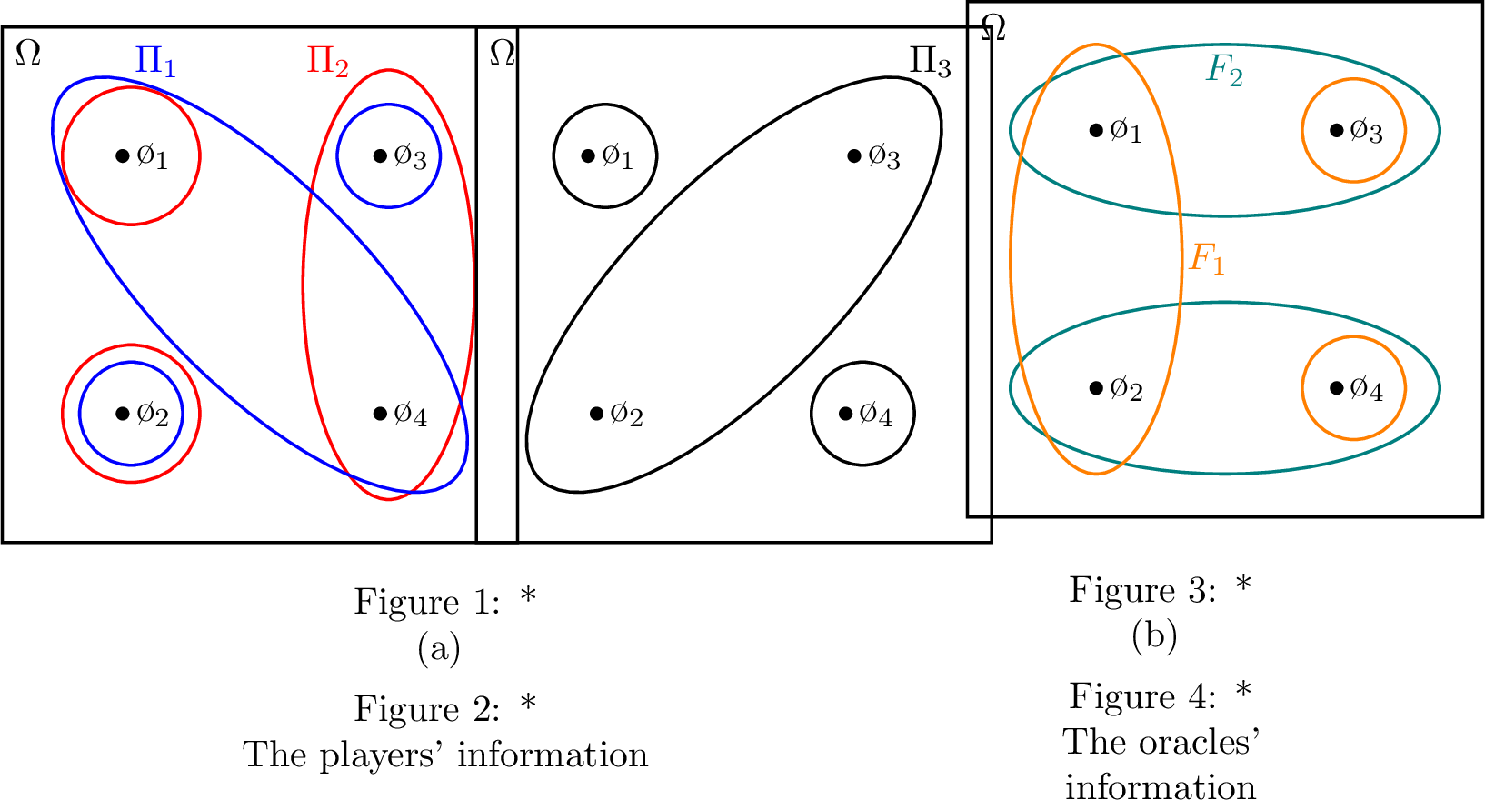
To see that JMI does not imply refinement in every CKC, consider the information structure described in Figure 3. Both oracles can either withhold all information or fully disclose their information, thereby ensuring that all players become fully informed of the realized state. In fact, these are all the possible experiments of Oracle \(2\). On the other hand, Oracle \(1\) can also signal the partition \(F_1'=\{\{{\omega}_1,{\omega}_2,{\omega}_3\},\{{\omega}_4\}\}\), which provides complete information to players \(1\) and \(2\) but provides no information to player \(3\). Thus, Oracle \(1\) is JMI than Oracle \(2\), while neither of the two partitions is finer than the other.

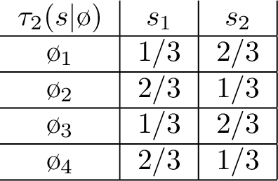
Another aspect of this example, which resonates with the key insight of the general analysis, is that there exists a stochastic experiment \(\tau_2\) that Oracle \(1\) cannot imitate. Specifically, consider the stochastic experiment \(\tau_2\) given in Figure 4. One can verify that there exists no \(\tau_1\) that yields the same profiles of posteriors as the stated experiment \(\tau_2\), and this hinges on the fact that \(F_1\) does not refine \(F_2\).

The key issue is that in the deterministic case each state is associated with a unique public signal, so JMI guarantees coincidence of the entire profile of posteriors and hence of the induced Bayesian game. Under stochastic experiment, however, each state can generate multiple signals with different weights, so the same partitions can induce different joint posteriors. This richer structure is not fully captured by players’ interim partitions (i.e., given any deterministic information conveyed by the oracles), and creates both within‑CKC and across‑CKC difficulties that require stronger conditions than JMI.

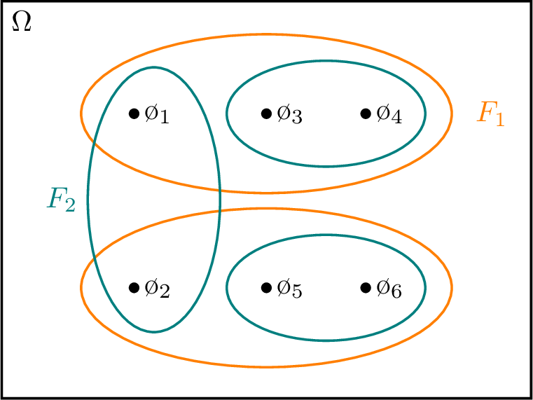
To demonstrate that refinement in every CKC does not imply JMI, consider the following example with two players whose partitions are \(\Pi_1=\{\{\omega_1,\omega_2\}, \{\omega_4, \omega_5\}, \{\omega_3, \omega_6\}\}\) and \(\Pi_2=\{\{\omega_1,\omega_2\}, \{\omega_3, \omega_4\}, \{\omega_5, \omega_6\}\}\). In this case, there are two CKCs, \(\{\omega_1,\omega_2\}\) and \(\{\omega_3,\omega_4,\omega_5,\omega_6\}\). Next, assume the two oracles have the following partitions, \(F_1=\{\{\omega_1,\omega_3,\omega_4\}, \{\omega_2,\omega_5,\omega_6\}\}\), \(F_2=\{\{\omega_1,\omega_2\}, \{\omega_3,\omega_4\}, \{\omega_5,\omega_6\}\}\), as illustrated in Figure 5. Observe that in every CKC, \(F_1\) refines \(F_2\).

Now consider a completely revealing, deterministic experiment \(\tau_2\) that maps the three different partition elements of \(F_2\) to three different signals: \(\tau_2(s_1|\omega_1)=\tau_2(s_1|\omega_2)=1\), \(\tau_2(s_2|\omega_3)=\tau_2(s_2|\omega_4)=1\), and \(\tau_2(s_3|\omega_5)=\tau_2(s_3|\omega_6)=1\). Can Oracle \(1\) produce an experiment \(\tau_1\) such that \(\Pi_i\vee \tau_1\) = \(\Pi_i\vee \tau_2\) for every player \(i\)?

Note that under \(\tau_2\), neither player can distinguish \(\omega_1\) from \(\omega_2\). Therefore, in order for \(\tau_1\) to satisfy \(\Pi_i\vee \tau_1\) = \(\Pi_i\vee \tau_2\) for every \(i\), the experiment \(\tau_1\) must map all \(F_1\) partition elements to the same signal. Consequently, under \(\tau_1\), Player 1 cannot distinguish \(\omega_4\) from \(\omega_5\), which is achievable given \(\tau_2\). We therefore conclude that Oracle 1 is not JMI than Oracle 2, even though \(F_1\) refines \(F_2\) in every CKC. However, in the special case where \(\Omega\) consists of a single CKC, refinement does imply JMI.

7.3.1 Two-sided JMI implies equivalence in every CKC↩︎

Though we substantiated that an JMI oracle need not have a finer partition in every CKC, this does hold in case both oracles dominate one another, under deterministic signaling strategies. The following corollary provides this equivalence by stating that, given a specific CKC, both oracles dominate each other if and only if their partitions coincide.

By applying the result within each CKC, the corollary asserts that the partitions \(F_1\) and \(F_2\) are equivalent in every CKC if and only if they are mutually JMI within that CKC, given any fixed set of players’ partitions. As a result, the issue of CKCs arises naturally in the context of deterministic oracles and becomes even more significant when studying stochastic ones, as examined in the stochastic analysis above.

8 Conclusion↩︎

This paper develops a comparative theory of generators of public information in incomplete-information games. We study an external oracle endowed with a partition of the state space who provides public signals to players holding heterogeneous private information. Signals must be measurable with respect to the oracle’s partition, so each signaling scheme induces a Blackwell experiment. Fixing players’ information structures and the prior, we introduce a dominance relation over oracles based on their ability to replicate each other’s sets of equilibrium outcome distributions across all games. This extends [1] from decision problems to incomplete-information games and from single experiments to generators of experiments. Oracle dominance further connects to Aumann’s theory of common knowledge through the central roles of CKCs and information loops.

The main conceptual object is the information loop. Local refinement inside each CKC is necessary for stochastic dominance, but it is not sufficient once the oracle’s partition connects several CKCs. Loops create global measurability constraints: the local experiments that mimic another oracle inside different CKCs must be glued into a single oracle-measurable public experiment. Covers and order-preserving covers describe when these loop constraints can be reproduced by the other oracle.

Using this geometry, we characterize oracle equivalence (mutual dominance) via two-sided refinement and order-preserving covers (Theorem 1). For one-sided stochastic dominance, we prove that dominance implies refinement within each CKC and that every loop of the dominating oracle must be covered by loops of the dominated one; when the relevant cover is unique, it must preserve cyclic order (Theorem 2). Conversely, refinement together with order-preserving covers is sufficient under separated-loop structures. The benchmark cases then follow naturally: with a unique CKC, or with no \(F_1\)-loops, dominance reduces to refinement inside CKCs (Corollary 1); non-informative loops and the two-CKC case provide additional tractable environments.

For deterministic experiments, dominance is equivalent to being jointly more informative: Oracle 1 can match every player’s posterior partition induced by any deterministic signaling scheme of Oracle 2 (Proposition 3). This deterministic result is a useful boundary case, but the stochastic analysis shows that public information in strategic environments cannot be ranked solely by local informativeness. Global measurability constraints across CKCs, captured by information loops, determine which joint beliefs and hence equilibrium outcomes are implementable.

9 Proofs↩︎

Appendix 9 is organized as follows. We first isolate three primitive tools: posterior mimicry, local refinement inside a single CKC, and the graph-theoretic form of loop compatibility. The proofs of the main results then cite these primitive tools when needed.

9.1 Posterior mimicry and local refinement↩︎

The following separation device is used only for necessity statements. It is a compact version of the proportionality argument used throughout the text.

The last supporting lemma states that refinement within every CKC is a necessary condition for dominance.

9.2 Loop algebra↩︎

The cover condition has a useful algebraic characterization. The next definition is mainly a test for coverability: it asks whether every binary \(F_{-i}\)-measurable split of the loop has the same number of transitions in the two directions.

Figure 6 (a) depicts an \(F_1\)-loop with three CKCs. Panel (b) shows a binary \(F_2\)-measurable split of this loop into \(A=\{\omega_1, \omega_2, \omega_3\}\) and \(B=\{\overline{\omega}_1, \overline{\omega}_2, \overline{\omega}_3\}\). Since \(\#(A\to B)=3\) and \(\#(B\to A)=0\), the loop is not \(F_2\)-balanced and therefore, by Proposition 4, not \(F_2\)-covered.

The third part of Proposition 4, combined with Eq. 1 , shows that covers are exactly the configurations under which every \(F_2\)-measurable likelihood-ratio product is neutral around the loop, and are therefore necessary for dominance.

9.3 Proof of Proposition 1↩︎

9.4 Necessity of loop covers↩︎

9.5 Constructive sufficiency tools↩︎

9.6 Proof of Theorem 1↩︎

9.7 Proof of Theorem 2↩︎

9.8 Proof of Corollary 2↩︎

9.9 Proof of Proposition 2↩︎

9.10 Proof of Proposition 3↩︎

9.11 Proof of Corollary 3↩︎

10 Online appendix↩︎

10.1 More than one CKC↩︎

As the benchmark corollaries below show, under a unique CKC, the partition-refinement condition ensures that Oracle \(1\) can produce the exact same experiment as Oracle \(2\). This conclusion, however, hinges on the existence of a unique CKC. In case there are several CKCs, Oracle \(1\) may need to follow a different experiment in order to match the distribution on posteriors generated by \(\tau_2\). Namely, \(\tau_1\) may require more signals than \(\tau_2\), even if both oracles have the same (complete) information in every CKC. Let us provide a concrete example for this.

Consider a uniformly distributed state space \(\Omega =\{{\omega}_1,{\omega}_2,{\omega}_3,{\omega}_4\}\), with two players whose private information is \(\Pi_1=\{\{{\omega}_1,{\omega}_2\},\{{\omega}_3\},\{{\omega}_4\}\}\) and \(\Pi_2=\{\{{\omega}_1\},\{{\omega}_2\},\{{\omega}_3,{\omega}_4\}\}\). The oracles have the following partitions \(F_1 = \{\{{\omega}_1,{\omega}_3\}, \{{\omega}_2\},\{{\omega}_4\}\}\) and \(F_2 = \{\{{\omega}_1\},\{{\omega}_3\}, \{{\omega}_2,{\omega}_4\}\}\). Notice that there are two CKCs, \(\{{\omega}_1,{\omega}_2\}\) and \(\{{\omega}_3,{\omega}_4\}\), and both oracles have complete information in each of these components. That is, \(F_1\) refines \(F_2\) in every CKC, and vice versa.

Consider the experiment \(\tau_2\) given in Figure 7. Notice it is \(F_2\)-measurable, as \(\tau_2(s|{\omega}_2)=\tau_2(s|{\omega}_4)\) for every signal \(s\), but not \(F_1\)-measurable.

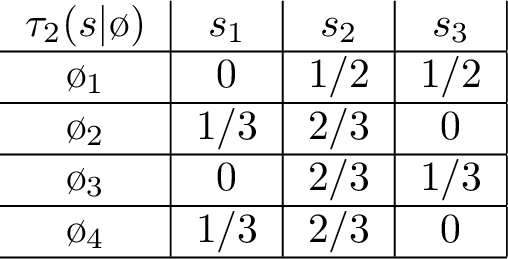
The set of \(\tau_2\)-posteriors \({\rm Post}(\tau_2)\) is \[{\rm Post}(\tau_2) = \left\{\!\begin{align} &(e_i, e_i), && \forall \;1 \leq i \leq 4, \\[1ex] &\left(\left(\tfrac{3}{7}, \tfrac{4}{7}, 0, 0\right), e_j\right), && j = 1, 2, \\[1ex] &\left(e_k, (0, 0, \tfrac{1}{2}, \tfrac{1}{2})\right), && k = 3, 4 \end{align}\right\},\] where the \(i^{\rm{th}}\) coordinate of \(e_i\) is \(1\), and we can now try to mimic \(\tau_2\) using an \(F_1\)-measurable experiment. First, this requires at least two signals to distinguish between \({\omega}_1\) and \({\omega}_2\), as well as \({\omega}_3\) and \({\omega}_4\). Second, the posterior \(\left(\left(\tfrac{3}{7}, \tfrac{4}{7}, 0, 0\right), e_1\right)\) requires another signal \(s\) so that \(\tau(s|{\omega}_1)=\alpha >0\) and \(\tau(s|{\omega}_3)=\tfrac{4}{3}\alpha >0\). However, the \(F_1\)-measurability requirement implies that \(\tau(s|{\omega}_3)=\alpha\), and the \(\tau_2\)-posterior \(\left(e_3, (0, 0, \tfrac{1}{2}, \tfrac{1}{2})\right)\) necessitates that \(\tau(s|{\omega}_4)=\alpha\) as well. These conditions are given in Table \((a)\) within Figure 8.

Evidently, it must be that \(\alpha,\beta,\gamma >0\) in order to mimic \(\tau_2\), but the second and fourth rows in Table (a) cannot jointly sum to \(1\) unless \(\alpha=0\), which eliminates the possibility of a well-defined mimicking experiment. Thus, in order to mimic the stated experiment \(\tau_2\), Oracle \(1\) requires an additional signal as presented in Table \((b)\), in Figure 8. To conclude, though the oracles’ partitions refine one another in every CKC, they cannot always produce the exact same experiment when trying to mimic each other.

10.2 Balancedness and the likelihood-ratio obstruction↩︎

This subsection contains the longer motivation for the cover criterion used in Section 4.2. Consider a non-balanced \(F_1\)-loop as in Figure 6 (b), and suppose that \(A\) and \(B\) are \(F_2\)-measurable sets with \(\#(A\to B)\neq \#(B\to A)\). For example, if \(A=\{\omega_1,\omega_2,\omega_3\}\) and \(B=\{\overline{\omega}_1,\overline{\omega}_2,\overline{\omega}_3\}\), then \(\#(A\to B)=3\) and \(\#(B\to A)=0\). Let \(s\) be a signal and define an \(F_2\)-measurable experiment by \[\tau_2(s\mid\omega)=\frac{1}{2}-\frac{1}{4}\mathbf{1}_{\{\omega\in A\}}.\] Then each transition from \(A\) to \(B\) contributes the likelihood ratio \(1/2\), and each transition from \(B\) to \(A\) contributes the likelihood ratio \(2\). Hence the product of likelihood ratios around the loop is \[\prod_j \frac{\tau_2(s\mid\omega_j)}{\tau_2(s\mid\overline{\omega}_j)} =2^{\#(B\to A)-\#(A\to B)},\] which is not equal to one whenever the loop is not balanced.

By contrast, any \(F_1\)-measurable experiment \(\tau_1\) must satisfy \[\prod_j \frac{\tau_1(s\mid\omega_j)}{\tau_1(s\mid\overline{\omega}_j)}=1,\] because \(\overline{\omega}_j\) and \(\omega_{j+1}\) are in the same \(F_1\)-atom. Thus Oracle 1 cannot match the likelihood-ratio restrictions generated by such a \(\tau_2\). This is the likelihood-ratio obstruction behind Proposition 4: balancedness is exactly the algebraic condition that rules out this obstruction, and the proposition shows that it is equivalent to the geometric condition of being covered by \(F_2\)-loops.

References↩︎