Sigma-Delta Neural Network Conversion on Loihi 2
May 09, 2025
Abstract
Neuromorphic computing aims to improve the efficiency of artificial neural networks by taking inspiration from biological neurons and leveraging temporal sparsity, spatial sparsity, and compute near/in memory. Although these approaches have shown efficiency gains, training these spiking neural networks (SNN) remains difficult. The original attempts at converting trained conventional analog neural networks (ANN) to SNNs used the rate of binary spikes to represent neuron activations. This required many simulation time steps per inference, which degraded efficiency. Intel’s Loihi 2 is a neuromorphic platform that supports graded spikes which can be used to represent changes in neuron activation. In this work, we use Loihi 2’s graded spikes to develop a method for converting ANN networks to spiking networks, which exploits temporal and spatial sparsity. We evaluated the performance of this network on Loihi 2 and compared it to NVIDIA’s Jetson Xavier edge AI platform. The results show that neuromorphic approaches achieve significant improvements in efficiency and latency (energy-delay product) over existing solutions.
<ccs2012> <concept> <concept_id>10010147.10010257.10010293</concept_id> <concept_desc>Computing methodologies Neural networks</concept_desc> <concept_significance>500</concept_significance> </concept>
<concept> <concept_id>10010147.10010257.10010321</concept_id> <concept_desc>Computing methodologies Machine learning</concept_desc> <concept_significance>300</concept_significance> </concept> </ccs2012>
1 Introduction↩︎
The increasing demand for more energy-efficient artificial intelligence systems has spurred the development of neuromorphic computing, an approach inspired by the structure and function of biological neurons. This field aims to enhance computational efficiency by leveraging principles such as temporal sparsity, spatial sparsity, and integrating compute capabilities near or within memory units. Unlike conventional AI computing architectures, which use globally accessible memory to perform dense matrix operations, neuromorphic systems keep compute near memory and process inputs as a stream of sparse, discrete spikes routed between neurons. These spiking neural networks (SNN) can reduce unnecessary computations by only transmitting spikes when there are significant changes to their input. SNNs also minimize energy use by only communicating between neurons selectively and by keeping memory close to computation units, reducing data movement and latency.
One notable hardware realization of these principles is Loihi[1], Intel’s neuromorphic processor for low-power, event-driven computations. The Loihi 2 [2] chip used in this work comprises 120 neuromorphic cores with each core supporting \(\sim\)8k neurons. Each neuromorphic core holds its associated neuron’s weights and internal state in local SRAM, enabling low-latency data storage. Loihi chips can be networked on a board to pass spikes between them and execute larger networks. Loihi 2’s neurons can execute custom microcode, allowing researchers to implement specialized neuron types tailored to specific applications. Each Loihi 2 chip is 31 mm² and is deployed on either the single-chip “Oheo Gulch" board, the 8-chip”Kapoho Point" board or the 16-chip VPX board which is used in these experiments. Built on the Intel 4 process, Loihi 2 use much less than 1 Watt per chip.
Training SNNs with binary spikes to accuracies comparable to conventional deep analog neural networks (ANN) has proven challenging, in part because the loss must be back-propagated over time [3]. In our experiments, training a spiking network takes \(\sim10\times\) the time as an ANN with the same architecture (Section 4.2). Attempts to convert trained ANNs to SNNs have largely used the rate of spikes to represent activation values [4]. This approach requires many timesteps per input to accurately estimate output spike rates. Loihi 2’s support for quantized graded spikes enables converting an ANN to a quantized
graded-spike SNN that takes advantage of temporal and spatial sparsity while being easy to train. Loihi’s graded spikes can hold up to 16 bit signed integer payloads which can represent quantized activations. This approach was inspired by the sigma-delta
neural network (SDNN) [5]. SDNNs accept incoming spikes representing changes in the activation of the previous layer, apply learned
weights, update their internal state, and then pass the change in their state to the next layer if it is larger than a given threshold. Their operation closely mirrors that of a conventional ANN neuron (Fig. 1). By
updating their state only when the input changes, SDNNs naturally exhibit temporal sparsity. Additionally, their selective activation of a limited subset of neurons ensures spatial sparsity, reducing power consumption, and improving resource efficiency.
Our contributions are summarized as follows:
\(\bullet\) We propose a novel method to convert trained artificial neural networks (ANNs) into Sigma-Delta Neural Networks (SDNNs).
\(\bullet\) We deploy the converted network on Loihi 2 in the field demonstrating the feasibility of running converted SDNNs on neuromorphic hardware.
\(\bullet\) We benchmark the converted network running on Loihi 2 against the original ANN network running on a Jetson Xavier edge AI accelerator and show that neuromorphic approaches achieve substantial improvements in
energy-delay product.

2 Related Works↩︎
O’Connor and Welling introduced SDNNs to reduce redundant computations by transmitting only changes in activation [5]. This temporal difference encoding allows for computational savings while maintaining network performance. Shrestha et al. [6] implemented an SDNN on Intel’s Loihi 2 and benchmarked its performance against an NVIDIA Jetson platform. Their work demonstrated the potential advantages of neuromorphic hardware for SDNNs by taking advantage of Loihi 2’s event-driven processing. However, their approach relied on SLAYER [7], a training framework designed for binary spiking networks. SLAYER requires the entire time series to be stored in memory during training. We found that this makes SDNN training more difficult and slower than conventional ANN training. Yousefzadeh et al. developed a method for converting ANNs to SDNNs [8], but this method still relied on binary spikes and was not compatible with modern model quantization approaches. In contrast, our approach can convert ANN networks trained and quantized with conventional pytorch tools to SDNNs capable of being deployed on Intel’s Loihi 2 neuromorphic hardware.
3 Methodology↩︎
3.1 Conversion and Implementation on Loihi 2↩︎
Loihi 2’s neurocores are only capable of integer arithmetic, so the network needs to be quantized. Instead of developing our own quantization approach, we aimed to make our ANN-SDNN conversion method compatible with standard quantization schemes. We started with PyTorch’s post-training static quantization [9] which converts the weights (\(w\)) and activations (\(x\)) from floating-point (FP32) to 8-bit integer (\(w_q\), \(x_q\)), while biases (\(b\)) were maintained in FP32. The quantization used an affine mapping defined by a floating-point scale (\(s\)) and an integer zero-point (\(z\)) for each tensor \(x_{float}=s\times(x_q-z)\) for activations and similarly for weights \(w_{float}=w\times(w_q-z)\). In PyTorch, the matrix multiplication is performed in integer arithmetic and the resulting integer accumulator is rescaled and combined with the FP32 bias before being re-quantized for processing by the next layer. The effective floating-point computation performed is: \(y_{float i,k}=k\sum (x_{q,ik}-z_x)\times(w_{q,jk}-z_w))\times(s_x \times s_w)+b_{float,j}\).
For deployment on Loihi 2, direct application of the floating-point scales is not possible. The version of the sigma-delta neuron microcode developed by Intel only allows rescaling by powers of two (bit-shifts). To maintain compatibility with the PyTorch quantization scales, we needed to modify the sigma-delta neuron microcode. We extracted the per-layer input scale (\(s_x\)), weight scale (\(s_w\)), and output scale (\(s_y\)) from the quantized PyTorch model using custom python code. The necessary rescaling factor for a layer, \(R=s_y \times s_x \times s_w\), was then implemented in the Loihi 2 microcode using fixed-point arithmetic. Specifically, the 24-bit accumulated pre-activation value within the neuron was multiplied by a pre-computed 24-bit integer scaling factor (\(scale\)) derived from \(R\), and subsequently right-shifted by a pre-computed exponent (\(scale_{exp}\)) to approximate the division by \(s_y\). The Loihi 2 microcode then implemented \(y=(accumulator \times scale)>>scale_{exp}\) to ensure the result remained within an 8-bit range for the next layer’s input, preventing overflow in the next layer’s 24-bit accumulator. The bias was similarly rescaled during conversion and added to the accumulator before scaling. This method was inspired by Jacob et al. [10]. The full redesigned microcode is shown in pseudocode in Algorithm 2. Our method deploys the converted model on Loihi 2 using an initial delta layer executing on the CPU to produce graded delta spikes from a sequence of RBG frames [0, 255] where \(spike_i = frame_i - frame_{i-1}\). The spikes are passed to Loihi 2 which performed the convolution operation and the sigma-delta neurons. The resulting spikes are received from Loihi 2 and added to a running sum to calculate output activations. These output activation frames were then dequantized using the final layer scaling factor from the quantized PyTorch model. These floating point outputs are interpreted as a YOLOv3-style grid of \(14\times14\) cells each with associated x-y locations and probability scores for each of the 3 bounding boxes (Fig. 1C). In our work, we leveraged nxkernel (v0.3.0) to deploy the model on Loihi 2, enabling more efficient mapping of our architecture to the hardware and better utilization of its event-driven computation capabilities. Inference was run in fall-through mode which runs 16 SNN simulation timesteps for each input and thereby allowing spikes to propagate through the network and corresponding output. This contrasts with nxkernel’s pipelined mode in which a new frame enters the network at each timestep and each layer of the network processes a different frame each step. Selecting fall-through mode gives us a dramatic advantage in latency for a small cost in throughput.

3.2 Dataset↩︎
We chose drone-detection in ground-based video as our first test application for our ANN-SDNN conversion pipeline because these videos have high temporal sparsity, with few moving objects. Drone detection is also a highly relevant application for this context because low-power video inference could enable low-power persistent sensors to watch the sky for enemy drones. We used the multi-sensor drone detection dataset [11] which includes 285 RGB videos, which have a resolution of 640\(\times\)512. We resized all input frames to fit the network input size of 448\(\times\)448. The dataset features four manually labeled classes of flying objects: drones, airplanes, helicopters, and birds. The sensor-to-target distance for drones ranged from 20 to 200 meters, and all video acquisitions were performed under daylight conditions. The videos were divided into training and test sets with 20\(\%\) reserved for testing.
In order to directly compare ANN-SDNN converted networks with SDNNs that had been directly trained with SLAYER, we used the Driving dataset [12], [13] which was used by Intel as a demonstration of SLAYER and Loihi 2’s ability to run efficient SDNNs [6]. This dataset is used to predict the steering angle of a vehicle based on the input from a dashboard RGB camera. It consists of images from a front-facing camera in a data collection vehicle coupled with the time-synchronized steering angle recorded from a human driver. All input frames were resized to match the PilotNet network’s required input resolution of 66\(\times\)200\(\times\)3.
| PilotNet | YOLO-KP | |
|---|---|---|
| Type | Conv/FC | Conv |
| Application | Angle Pred. | Obj. Detection |
| Parameters | 0.35M | 3.4M |
| Neurons | 12K | 2M |
| Loihi Chips | 1 | 5 |
4pt
3.3 Model and Training↩︎
The model architecture used for drone detection (YOLO-KP) was developed by Intel and based on the YOLO v3-Tiny architecture [14]. It was adapted to accommodate the memory and architectural constraints of Loihi 2. The most important consideration for Loihi 2 is minimizing the number of neurons. Each Loihi 2 core can hold only a fixed number of neurons as each requires designated dendrite and axon resources. Therefore, higher resolution and deeper networks require more Loihi 2 chips which in turn consume more power. For this reason, max-pooling layers were replaced by strided convolutions for spatial down-sampling. Residual layers were similarly removed to reduce memory requirements and eliminate the need to synchronize spikes arriving from different layers. These removals greatly simplified the implementation. The model in the lava-nc/lava-dl github repository [15] has been used as the basis for other works benchmarking video object detection on Loihi [16]. The PilotNet model used for the Driving dataset had an identical architecture to Intel’s SLAYER trained model [6] and was small enough that it was able to run on a single Loihi chip. Model summaries are shown in Table 1.
In order to demonstrate the flexibility of our ANN-SDNN conversion approach, we trained the ANN model using student-teacher distillation. We first trained a MobileNetV2 [17] based teacher model on the same dataset. We then employed a masked L2 feature matching loss to align the penultimate layer representations between the teacher (MobileNetV2) and student (YOLO-KP) models. This feature distillation loss was combined with the standard detection loss using a weighting coefficient \(\alpha\) = 0.069, allowing the student network to simultaneously optimize for detection performance while mimicking the richer feature representations learned by the teacher model. The model hyper-parameters were tuned with Optuna. We used the albumentations package for data augmentation, Adam optimizer, Reduce-on-plateau learning rate scheduler and trained for 30 epochs. The model was quantized to 8-bit per-tensor using PyTorch with HistogramObserver (activations) and MinMaxObserver (weights).
3.4 Accuracy-Sparsity Tradeoff Exploration↩︎
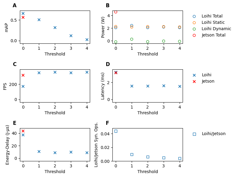
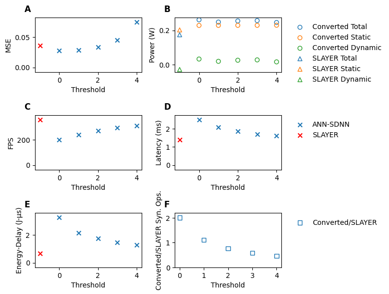
SDNNs control sparsity by tuning the threshold for propagating changes to the next layer. When the thresholds are set to zero, the cumulative output exactly matches the quantized network. When thresholds are increased, only larger changes are passed through the network. This decreases the number of spikes and the number of synaptic operations needed to execute the network while sacrificing accuracy that exists in the original quantized ANN. In order to explore this tradeoff, we raised the threshold from 0 to 4 for the converted YOLO-KP and PilotNet networks starting from the initial delta layer and the results are shown in Fig. 3 and Fig. 4 respectively. This gave us a spectrum from the minimum sparsity and highest accuracy to higher sparsity and lower accuracy.
3.5 Benchmarking Loihi 2↩︎
Our experiments were run on an in-house Loihi VPX development board containing 16 Loihi 2 chips and associated IO electronics and connected by 1 and 10 Gigabit Ethernet for control and data respectively. In order to measure the power and latency of the Loihi 2 board, we used the nxkernel API’s built in profiling probes that report the power usage, timing, and core-level activity measurements. These probes measured static and total power. Following the format of Shrestha et al.[6], we report static, dynamic, and total power. Static power is calculated only from the chips that were used by the network. The dynamic power was calculated as the measured total power minus measured static power. The reported total power is the sum of the adjusted static power and the dynamic power.
Since integrated circuit design can generally trade speed for energy-efficiency, the energy-delay product (EDP) is used as a measure of overall efficiency of an integrated circuit [18]. The EDP reported here is calculated as \(power \times timestep \times latency\). Measurements of the accuracy of Loihi 2 were performed separately by running the entire test set through the Loihi 2 board, saving the output spikes, and then evaluating the accuracy after the run. In order to better understand how IO impacts the execution speed of Loihi 2 in our applications, we loaded 100 frames into on-chip memory and replayed these 10,000 times in order to measure power and latency in the absence of any IO bottlenecks (Fig. 5). This approach for reporting power, latency, and EDP is consistent with Intel’s recommended reporting structure for Loihi benchmarks [6].
3.6 Benchmarking NVIDIA Jetson↩︎
To compare our results on Loihi with conventional approaches, we ran the same network as an 16-bit floating point ANN on an NVIDIA Jetson Xavier edge AI board using the TensorRT library. The tegrastats tool provided by NVIDIA was used for power measurement and the VDD_CPU_GPU_CV and VDD_SOC power channels were combined to estimate the total power used for network execution. It should be noted that tegrastats on Xavier was not capable of measuring the power used solely by the GPU. Therefore, the comparison between the Xavier and Loihi 2 is not an identical comparison since we report only the power used by the Loihi 2 chip but must report the power used by the whole system-on-chip (SOC) in the case of the Xavier. This choice was made to be consistent with Intel’s comparisons to a similar Jetson device[6]. To separate GPU execution from CPU preprocessing, initialization and preprocessing were performed first, then execution was paused and resumed using TensorRT. The network was run with a batch size of 1 inside a python for-loop without the system GUI running.
4 Results↩︎
4.1 Model Accuracy↩︎
The MobileNetV2 teacher model achieved a mean-average precision (mAP) of 0.72, while our knowledge-distilled student model (YOLO-KP) reached a higher mAP of 0.74. This performance improvement is notable considering that YOLO-KP without knowledge distillation never exceeded 0.6 mAP in our experiments. The comparable parameter count between YOLO-KP and MobileNetV2 likely contributed to the student model’s ability to effectively leverage the teacher’s representations. After quantization, the accuracy decreased modestly to 0.62 mAP. These results were calculated across our complete test set of 58 videos containing 18,214 frames. For context, the authors of the multi-sensor drone dataset reported mAP values ranging from 0.58 to 0.84 depending on target distance when using a larger, full-precision model [11]. For PilotNet, performance is evaluated using mean squared error (MSE) and the configuration with threshold 0 achieves the lowest MSE of 0.0278.

4.2 SLAYER Training Comparisons↩︎
In order to compare the our ANN-SDNN conversion approach with Intel’s SLAYER training algorithm, we trained the YOLO-KP SDNN network with the same architecture on the same Multi-Sensor Drone Detection Dataset. Training was conducted for 50 epochs with a batch size of 16, a starting learning rate of \(2\times10^{-5}\) was used with a learning rate scheduler of factor 0.1. The results (Table 2) highlight significant improvements in both training efficiency and performance of our conversion approach. Our quantized model achieves higher mAP (0.62 vs 0.37) demonstrating better detection accuracy than SLAYER. Additionally, ANN training only took 5 minutes per epoch compared to 55 minutes for SLAYER on our NVIDIA GTX 4090. The conversion process only added 30 seconds for post-training quantization.
| Model | Time per Epoch (min) | Completion Time (hrs) | Memory | mAP |
|---|---|---|---|---|
| SLAYER | 55 | 45.80 | 9.4G | 0.37 |
| Our Approach | 5 | 3.40 | 8.6G | 0.62 |
3pt
| Model | Platform | Energy/frame (mJ \(\downarrow\)) | Latency (ms \(\downarrow\)) | Throughput (FPS \(\uparrow\)) | EDP (\(\mu Js\downarrow\)) |
|---|---|---|---|---|---|
| YOLO-KP SDNN | Loihi | 11.73 | 3.20 | 175.6 | 37.59 |
| YOLO-KP SDNN | Loihi no IO | 19.89 | 2.86 | 196.5 | 56.93 |
| YOLO-KP ANN | Jetson Xavier | 14.10 | 3.11 | 321.9 | 43.80 |
| PilotNet SDNN | Loihi | 1.31 | 2.50 | 200.2 | 3.26 |
| PilotNet SDNN | Loihi no IO | 1.06 | 1.13 | 442.9 | 1.20 |
| PilotNet ANN [6] | Jetson Nano | 21.94 | 5.77 | 173.2 | 126.20 |
| Energy Ratio(\(\downarrow\)) | Latency Ratio(\(\downarrow\)) | Throughput Ratio(\(\uparrow\)) | EDP Ratio (\(\downarrow\)) | ||
| YOLO-KP | 0.832 | 1.031 | 0.545 | 0.858 | |
| YOLO-KP (no IO) | 1.410 | 0.922 | 0.610 | 1.300 | |
| PilotNet | 0.060 | 0.433 | 1.156 | 0.026 | |
| PilotNet (no IO) | 0.0483 | 0.196 | 2.56 | 0.00948 |
4.3 Power, Latency, and Throughput↩︎
The results in Fig. 3, obtained from Loihi 2 activity probes show that the YOLO-KP SDNN had 0.056 of the synaptic operations as the ANN network and that, as expected, this ratio decreased as the threshold increased. Increasing the sigma-delta threshold from 0 to 4 increased the sparsity from 18\(\times\) to 250\(\times\) which improved the throughput from 176 FPS to 362 FPS. The total power usage was lower for Loihi 2 compared to the Jetson and remained relatively consistent for all experiments as it is dominated by static draw. The model running on Loihi 2 executes a single time step in 3.20 ms and uses 11.73 mJ of energy. The IO-constrained YOLO-KP SDNN on Loihi 2 achieves over 1.2\(\times\) lower EDP. The throughput and latency are somewhat worse than the Jetson Xavier which processes an entire frame in 3.1 ms and uses 14.1 mJ of energy (Fig. 3). For the unbottlenecked trials that avoided using IO, the speed increased to 2.86 ms per timestep and used 19.89 mJ of energy per inference (Fig. 5). For PilotNet, the SDNN implementation on Loihi 2 demonstrates substantial efficiency improvements over the ANN baseline on Jetson Nano. The Loihi-based PilotNet SDNN model achieves significantly lower energy per frame (1.31 mJ vs. 21.94 mJ) and reduced latency (2.50 ms vs. 5.77 ms), resulting in a much lower energy-delay product (3.26 \(\mu\)Js vs. 126.20 \(\mu\)Js). When I/O overhead is removed, performance improves further, with energy dropping to 1.06 mJ, latency to 1.13 ms, and throughput increasing to 442.9 FPS, yielding an EDP of just 1.20 \(\mu\)Js. A detailed performance comparison of Loihi 2 and Jetson for YOLO-KP and PilotNet at zero threshold is provided in Table 3. Overall, these results highlight the strong energy efficiency and latency advantages of the SDNN approach on Loihi 2 for PilotNet compared to conventional ANN deployment on edge GPUs.
4.4 Comparison with Intel’s published work↩︎
Intel has previously published work comparing PilotNet SDNN run on Loihi 2 with the same network run on an NVIDA Jetson Orin Nano accelerator[6]. In this study we re-ran Intel’s trained PilotNet SDNN using the recently released nxkernel API and found that the execution time was substantially improved. In our study, the SDNN implementation achieves lower energy per frame (1.31 mJ) and latency (2.50 ms) which further improves in the no-I/O configuration to 1.06 mJ and 1.13 ms, yielding a strong reduction in energy-delay product (EDP) from 3.26 \(\mu\)Js to 1.20 \(\mu\)Js. Intel’s results show a comparable energy figure under standard operation (1.26 mJ)[6], but significantly higher end-to-end latency (65.4 ms)[6], suggesting substantial I/O or system overheads in their pipeline. These results demonstrate the efficiency benefits of Loihi-based SDNNs, while highlighting that system integration and I/O overheads play a critical role in determining end-to-end performance.
4.5 Field Deployment at Silent Swarm 2025↩︎
To validate the feasibility of deploying the converted SDNN in an operational setting, the YOLO-KP network was deployed on the Loihi 2 VPX board at the US Navy’s Silent Swarm 2025 (SS25) experimentation event (Fig. 6). While the YOLO-KP architecture has previously been demonstrated on Loihi 2 for object detection from an airborne platform [16], a stationary ground-based sensor is a more natural fit for neuromorphic processing, as only the target moves within the field of view. The network was trained as an ANN on the IR video subset of the MSDD dataset and run on Loihi 2 in fall-through mode. The deployed system operated in real time, achieving 112 FPS with a latency of 5.0 ms and an energy consumption of 20 mJ per frame. These results demonstrate that ANN-to-SDNN conversion produces systems capable of sustained, real-time neuromorphic inference under field conditions; a non-trivial result given the added complexity of live data ingestion, hardware integration, and environmental variability absent from controlled benchmarks. Detection performance reflected the substantial domain gap between MSDD and SS25: a model trained on MSDD achieved 0.03 mAP on SS25 data, improving 10× to 0.30 mAP with minimal fine-tuning on a small SS25 subset. This rapid adaptation highlights the transferability of the ANN-to-SDNN conversion approach. The remaining performance gap reflects the presence of novel drone types, including vertical-takeoff-and-landing platforms, and greater background complexity not represented in the MSDD training set. The field conditions also introduced higher camera motion, resulting in reduced temporal sparsity (13% average sparsity after delta encoding versus 2% for MSDD), which accounts for the difference in efficiency metrics relative to the controlled benchmarks in Section 4.3

5 Discussion↩︎
We were successfully able to train ANN-based models for video understanding and control tasks, quantize them, and deploy them as SDNNs on Loihi 2. Across both YOLO-KP and PilotNet, the deployed networks leveraged significant sparsity gains relative to their ANN counterparts e.g. \(>18\times\) sparsity improvement for YOLO-KP compared to the original ANN (Fig. 3F). For both YOLO-KP and PilotNet, the Loihi 2 SDNN implementation substantially reduces energy per frame and energy-delay product compared to conventional ANN deployment, with PilotNet achieving over 16\(\times\) lower energy and \(\sim 40\times\) lower EDP. Loihi achieves competitive latency and throughput, with further improvements observed when I/O bottlenecks are removed and thresholds are increased. In comparing the two platforms, a key design choice of Loihi is the use of on-chip SRAM for all weights and activations. This reduces memory access latency but increases static power consumption, which scales with the number of Loihi chips and makes higher-resolution inputs more power-intensive.
The PilotNet results also allow a direct comparison between our conversion approach and SLAYER-trained SDNNs. Because our method converts standard quantized ANNs to SDNNs, it is fully compatible with conventional PyTorch training pipelines, enabling the use of off-the-shelf optimizers, data augmentation, and quantization tools without modification. This flexibility comes with an accuracy advantage: our converted PilotNet achieves lower MSE than the SLAYER-trained equivalent as shown in Fig. 4A, consistent with the YOLO-KP results. The converted network does exhibit somewhat lower sparsity than a SLAYER-trained model, since sparsity is not explicitly encouraged during training, but it nonetheless captures the majority of the efficiency benefits available from sparse neuromorphic execution.
Even if compilation and IO improvements are implemented to decrease the execution time of these networks on Loihi 2, traditional frame-based cameras may not fully leverage Loihi’s asynchronous event-driven architecture. Event-based cameras, with their near-continuous temporal resolution and inherent sparsity, could provide a more natural pairing with neuromorphic hardware like Loihi 2, potentially unlocking greater efficiency advantages for video analysis tasks. This complementary hardware approach may explain why lower resolution videos have shown more favorable comparisons with conventional accelerators [6]. Additionally, a larger single Loihi 2 chip could offer the key benefit of reducing costly inter-chip communications making spiking networks more attractive.
The authors thank Mark Barnell and Dr. Qing Wu (Air Force Research Laboratory) for providing the Loihi 2 board, and Intel’s Loihi team, especially Sumit Bam Shrestha, for their support. This work was supported by the U.S. Navy (N6833522C0487) and SRC/DARPA JUMP 2.0 PRISM Center.