1 Introduction↩︎

Covert communication ensures that the communication remains undetectable [1]–[4]. In a point-to-point classical DMC, it is well established that it is possible to reliably and covertly transmit at most \(O(\sqrt{n})\) bits over \(n\) channel uses [3], [4], provided that the encoder and decoder share a secret key of size \(O(\sqrt{n})\) bits [3]. Also, covert communication over discrete memoryless MACs is studied in [5], where each transmitter shares a secret key with the receiver. The authors show that each transmitter can transmit on the order of \(\sqrt{n}\) reliable and covert bits per \(n\) channel use. We note that positive covert communication rates can be achieved for point-to-point classical DMCs [4] only when the symbol \(x_0\in\mathcal{X}\), transmitted by the sender in the no-communication mode, is redundant, which implies that the distribution induced on the warden’s channel observation by \(x_0\in\mathcal{X}\) can also be induced using the channel input symbols \(\{x\in\mathcal{X}:x\ne x_0\}\). Building on this result, it has been demonstrated that positive covert rates can also be achieved over classical channels under various scenarios: (i) when a friendly jammer is present [6]–[9], (ii) when the transmitter has access to CSI [10]–[13], (iii) when the transmitter has access to ADSI [14], [15], (iv) when the warden has uncertainty about the statistical characteristics of its channel [16], [17], (v) and when there is a cooperative user who knows either the message or the transmitter’s codeword [7], [9], [15].

Existing works on covert communication over quantum channels show that optimal rates obey the square root law. Specifically, covert communication over bosonic channels is considered in [18], [19], where the authors demonstrate that the covert capacity adheres to the square root law. Additionally, [20]–[22] establish that the covert capacity of classical-quantum point-to-point channels also adheres to the square root law. We note that the availability of entangled qubits at both the transmitter and the receiver does not enable a positive covert rate [23].

In this paper, unlike previous works, we show that it is possible to achieve positive covert rates over a quantum three-user MAC when one of the transmitters has access to the private messages of the other two transmitters and aims to assist them in covertly communicating with the receiver. We present an achievable covert rate region for this problem. The special case of our achievable rate region for the classical and quantum channels recovers as a special case the known results for covert communication over classical MACs with degraded message sets [9], for communication over classical MACs with a helper [24]–[27], and communication over quantum MAC [28], [29].

Our achievability scheme relies on simultaneous pinching [30], superposition coding, and channel resolvability. Specifically, our reliability analysis is based on the pinching method, while our covertness analysis employs channel resolvability and pinching techniques [30], [31], which facilitate the channel resolvability analysis required to establish covertness. In particular, we derive a generalized channel resolvability lemma for quantum MACs with a helper.

Some related works that do not consider covertness constraint include: Classical MAC with general message sets is studied in [24], [26], [27]. Secure communication over MACs is studied in [32]. The problem of communication over MAC with cribbing is studied in [33], for classical channels, and studied in [34], for quantum channels. Also, secure communication and channel resolvability over classical MACs with cribbing is studied in [35] and secure communication over quantum state-dependent channels is studied in [36].

Notation: Let \(\mathbb{N}\) be the set of natural numbers and \(\mathbb{R}\) be the set of real numbers. For any \(x, y\in\mathbb{R}\), define \(\left[{x}{\,:\,}{y}\right] \triangleq [\lfloor x\rfloor, \lceil y \rceil]\cap \mathbb{N}\) and \([x] \triangleq \left[{1}{\,:\,}{x}\right]\). For a set of indices \(\mathcal{I}\subset\mathbb{N}\), \(M_\mathcal{I}\) denotes \((M_i)_{i\in\mathcal{I}}\). We denote the set of positive semi-definite operators on a finite-dimensional Hilbert space \(\mathcal{H}\) by \(\mathcal{P}(\mathcal{H})\) and denote the set of quantum states by \(\mathcal{D}(\mathcal{H})\triangleq\{\rho\in\mathcal{P}(\mathcal{H}):\mathop{\mathrm{Tr}}[\rho]=1\}\). We also denote the space of the bounded linear operators on \(\mathcal{H}\) with \(\mathcal{L}(\mathcal{H})\). For \(\rho,\sigma\in\mathcal{D}(\mathcal{H})\), the fidelity distance [37], [38] between these two quantum states is denoted by \(\mathop{\mathrm{F}}(\rho,\sigma)\triangleq\lVert\sqrt{\rho}\sqrt{\sigma}\rVert_1\), where \(\lVert\rho\rVert_1\triangleq\mathop{\mathrm{Tr}}\left[\sqrt{\rho^\dagger\rho}\right]\). For \(\rho,\sigma\in\mathcal{D}(\mathcal{H})\), the quantum relative entropy is defined as \(\mathbb{D}(\rho\lVert\sigma)=\mathop{\mathrm{Tr}}\left[{\rho\left({\log\rho-\log\sigma}\right)}\right]\). The identity operator on some Hilbert space \(\mathcal{H}\) is denoted by \(\mathbb{I}\). We use \(\tau\) to denote a quantum density matrix and use \(\ket{\tau}\) to denote the associated quantum state.

2 Problem Statement↩︎

2.1 One-Shot Regime↩︎

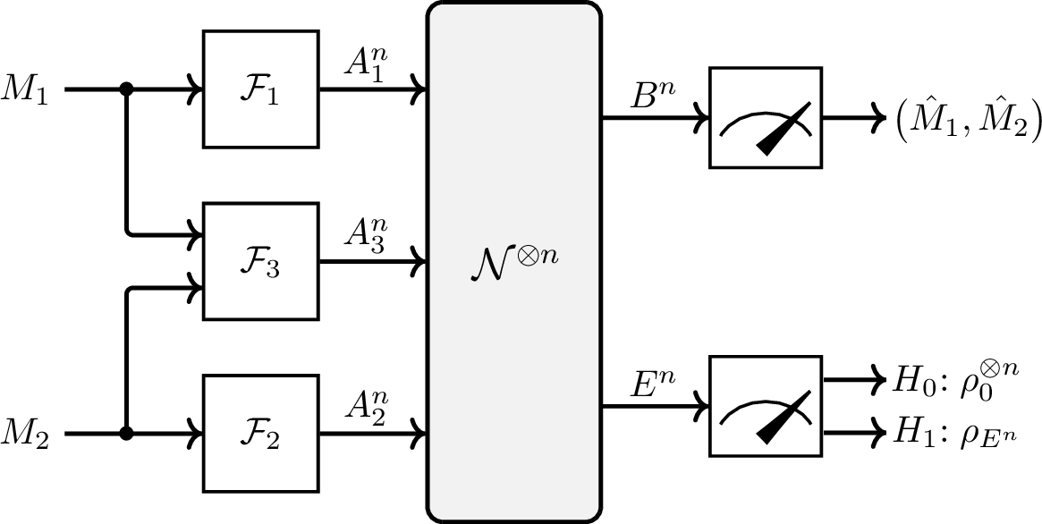
Fig. 1 illustrates a communication system designed for two transmitters to communicate covertly over a quantum MAC. In this setup, a helper, who has access to the private messages of the other transmitters, aims to aid them in covertly communicating with the legitimate receiver. We define codes as follows.

The code is known by all the terminals, and the objective is to design a reliable and covert code. From Definition 1 the output of the legitimate receiver’s channel is \[\tag{1} \begin{align} B=\mathop{\mathrm{Tr}}_E\mathcal{N}_{A_{[T]}\to BE}\left(\mathcal{F}_{[3]\to A_{[3]}}\right),\tag{2} \end{align}where \mathcal{F}_{[3]\to A_{[3]}}\triangleq\left\{\mathcal{F}_{t\to A_t}\right\}_{t\in[3]}. Therefore, from Definition~\ref{defi:code} and \eqref{eq:Legi95Output} the probability of error is defined as \begin{aligned} P_e&\triangleq\mathbb{P}\left\{(M_1,M_2)\ne(\hat{M}_1,\hat{M}_2)\right\}=\frac{1}{\left\lvert{\mathcal{M}_1}\right\rvert\left\lvert{\mathcal{M}_2}\right\rvert}\sum_{(m_1,m_2)\in\mathcal{M}_1\times\mathcal{M}_2}\mathop{\mathrm{Tr}}\left[\left(\mathbb{I}-\mathcal{D}^{\left(m_{[2]}\right)}_{B\to M_{[2]}}\right)(B)\right].\tag{3} \end{aligned}The code (2^{R_1},2^{R_2},1) is reliable if \begin{align} P_e&\le\epsilon.\tag{4} \end{align}\] When communication is not happening the transmitters transmit the innocent state \(\phi_0^{(t)}\in\mathcal{D}(\mathcal{H}_t)\) and therefore the warden receives the quantum state \[\begin{align} \rho_0\triangleq\mathop{\mathrm{Tr}}_B\mathcal{N}_{A_{[t]}\to BE}\left(\phi_0^{(1)}\otimes\phi_0^{(2)}\otimes\phi_0^{(3)}\right).\label{eq:No95Comm} \end{align}\tag{5}\]

Let \(\rho_{M_s}\), for \(s\in[2]\), denote the classical-quantum state corresponding to the message \(M_s\), which is \[\begin{align} \rho_{M_s}\triangleq\frac{1}{\left\lvert{\mathcal{M}_s}\right\rvert}\sum\limits_{m_s\in\mathcal{M}_s}\ket{m_s}{}\bra{m_s}.\label{eq:Message} \end{align}\tag{6}\] The state induced at the output of the warden by our code design is denoted by \(\tau_E\). Now we define the covertness metric as, \[\begin{align} \left\lVert\tau_E- \rho_0\right\rVert_1&\le\delta.\label{eq:Covertness95Metric} \end{align}\tag{7}\] The metric in 7 indicates that the state induced at the output of the warden should approximate the state induced at the output of the warden when communication is not happening, i.e., communication is covert.

2.2 Asymptotic Regime↩︎

We now define the problem in the asymptotic regime, where the channel is utilized \(n\) times independently as \(n\) approaches infinity. The corresponding \(\left(2^{nR_1},2^{nR_2}, n\right)\) code for the channel \(\mathcal{N}_{A_{[3]}\to BE}^{\otimes n}\) is similarly defined as Definition 1, with the message set \(\mathcal{M}_s\triangleq\left[\left\lfloor{2^{nR_s}}\right\rfloor\right]\), for \(s\in[2]\), quantum states \(A_{[3]}^n,B^n,E^n\in\mathcal{D}(\mathcal{H}^n)\). Then, the output of the legitimate receiver’s channel is \[\tag{8} \begin{align} B^n=\mathop{\mathrm{Tr}}_{E^n}\mathcal{N}_{A_{[3]}^n\to B^nE^n}\left(\mathcal{F}_{[3]\to A_{[3]}^n}\right),\tag{9} \end{align}where \mathcal{F}_{[3]\to A_{[3]}^n}\triangleq\left\{\mathcal{F}_{t\to A_t^n}\right\}_{t\in[3]}.Also, the probability of error is \begin{aligned} P_e^{(n)}&\triangleq\mathbb{P}\left\{(M_1,M_2)\ne(\hat{M}_1,\hat{M}_2)\right\}=\frac{1}{\left\lvert{\mathcal{M}_1}\right\rvert\left\lvert{\mathcal{M}_2}\right\rvert}\sum_{m_{[2]}\in\mathcal{M}_{[2]}}\mathop{\mathrm{Tr}}\left[\left(\mathbb{I}-\mathcal{D}^{\left(m_{[2]}\right)}_{B^n\to M_{[2]}}\right)\left(B^n\right)\right].\tag{10} \end{aligned}A sequence of codes \left(2^{nR_1},2^{nR_2}, n\right) is reliable if \begin{align} \lim_{n\to\infty}P_e^{(n)}&=0.\tag{11} \end{align}When communication is absent, the transmitter t\in[T] sends the innocent state \phi_{t,0}^n \in \mathcal{D}(\mathcal{H}_t^n), and consequently, the warden receives the quantum state \begin{align} \rho_0^{\otimes n}\triangleq\mathop{\mathrm{Tr}}_{B^n}\mathcal{N}_{A_{[T]}^n\to B^nE^n}^{\otimes n}\left(\phi_{1,0}^n\otimes\phi_{2,0}^n\otimes\phi_{3,0}^n\right).\tag{12} \end{align}\] Now we define the covertness metric as, \[\begin{align} \lim_{n\to\infty}\left\lVert\tau_{E^n}-\rho_0^{\otimes n}\right\rVert_1&=0.\label{eq:CC95CSK95Metric95Asymp} \end{align}\tag{13}\]

3 Main Results↩︎

3.1 One-Shot Results↩︎

Theorem 1 is proved in Section 4.

3.2 Asymptotic Results↩︎

Theorem 2 is proved in Section 7.

4 Proof of Theorem 1↩︎

We show that for each \(\delta_1,\delta_2,\epsilon>0\), there exists a \(\left({1,\epsilon,2^{R_1-\delta_1},2^{R_2-\delta_2}}\right)\) code for the quantum channel \(\mathcal{N}_{A_{[3]}\to BE}\) that satisfies both the reliability constraint and the covertness constraint. Fix \(p_{X_1},p_{X_2},p_{X_3\lvert X_1X_2}\) and \(\delta_1,\delta_2,\epsilon>0\).

4.1 Random Codebook Generation↩︎

Let \(C_1\triangleq\left\{{X_1(m_1)}\right\}_{m_1\in\mathcal{M}_1}\), where \(\mathcal{M}_1\triangleq\big[{2^{R_1}}\big]\), be a random codebook generated iid according to \(p_{X_1}\). A realization of \(C_1\) is denoted by \(\mathcal{C}_1\triangleq\left\{{x_1(m_1)}\right\}_{m_1\in\mathcal{M}_1}\).

Similarly, let \(C_2\triangleq\left\{{X_2(m_2)}\right\}_{m_2\in\mathcal{M}_2}\), where \(\mathcal{M}_2\triangleq\big[{2^{R_2}}\big]\), be a random codebook generated iid according to \(p_{X_2}\). A realization of \(C_2\) is denoted by \(\mathcal{C}_2\triangleq\left\{{x_2(m_2)}\right\}_{m_2\in\mathcal{M}_2}\).

Also, for every \(\mathcal{C}_1\), \(\mathcal{C}_2\), \(x_1\in\mathcal{C}_1\), and \(x_2\in\mathcal{C}_2\), let \(C_3\triangleq\big(X_3(m_1,m_2)\big)_{(m_1,m_2)\in\mathcal{M}_1\times\mathcal{M}_2}\), be a set of random codeword generated iid according to \(p_{X_3\lvert X_1X_2}(x_3\lvert x_1(m_1),x_2(m_2))\). A realization of \(C_3\) is denoted by \(\mathcal{C}_3\triangleq\big(x_3(m_1,m_2)\big)_{(m_1,m_2)\in\mathcal{M}_1\times\mathcal{M}_2}\). Also, let \(C\triangleq\left(C_1,C_2,C_3\right)\) and \(\mathcal{C}\triangleq\left(\mathcal{C}_1,\mathcal{C}_2,\mathcal{C}_3\right)\).

4.2 Encoding↩︎

To send the message \(m_t\), for \(t\in[2]\), the Transmitter \(t\) selects \(x_t(m_t)\), and prepares \(\rho_{A_t}=\theta^{x_t}\) and transmits it over the channel. Also, given \((m_1,m_2)\), the third transmitter computes \(x_3(m_1,m_2)\) and prepares \(\rho_{A_3}=\theta^{x_3}\) and transmits it over the channel. This encoding scheme induces the following state at the output of the warden \[\begin{align} &\tau_{E\lvert\mathcal{C}}\triangleq\frac{1}{2^{R_1+R_2}}\sum_{m_{[3]}}\rho_{E\lvert x_1\left({m_1}\right),x_2\left({m_2}\right),x_3\left({m_1,m_2}\right)}.\label{eq:Joint95Dist} \end{align}\tag{14}\]

4.3 Pinching↩︎

Our decoding procedure is based on the pinching method [30]. Consider states \(\sigma\in\mathcal{D}(\mathcal{H})\) and \(\rho\in\mathcal{D}(\mathcal{H})\), and let \(\sigma=\sum_{i}\lambda_i\ket{z_i}{}\bra{z_i}\) be the spectral decomposition of the state \(\sigma\). The pinching operation of the state \(\rho\) wrt the spectral decomposition of the state \(\sigma\) is defined as \(\Delta_\sigma(\rho)\triangleq\sum_i\ket{z_i}{}\bra{z_i}\rho\ket{z_i}{}\bra{z_i}=\sum_i\bra{z_i}\rho\ket{z_i}\ket{z_i}{}\bra{z_i}\). Note that the state \(\sigma\) and the state \(\Delta_\sigma(\rho)\) commute. Now consider the following classical-quantum states, \[\begin{align} &\rho_{X_{[3]}B}\triangleq\sum_{x_{[3]}}p_{X_1}(x_1)p_{X_2}(x_2)p_{X_3\lvert X_1X_2}(x_3\lvert x_1x_2)\ket{x_1}{}\bra{x_1}_{X_1}\otimes\ket{x_2}{}\bra{x_2}_{X_2}\otimes\ket{x_3}{}\bra{x_3}_{X_3}\otimes\rho_{B\lvert x_{[3]}},\tag{15}\\ &\rho_{(X_2,X_3)-X_1-B}\triangleq\sum_{x_{[3]}}p_{X_1}(x_1)\ket{x_1}{}\bra{x_1}_{X_1}\otimes\rho_{X_2 X_3\lvert x_1}\otimes\rho_{B\lvert x_1},\tag{16}\\ &\rho_{(X_1,X_3)-X_2-B}\triangleq\sum_{x_{[3]}}p_{X_2}(x_2)\ket{x_2}{}\bra{x_2}_{X_2}\otimes\rho_{X_1 X_3\lvert x_2}\otimes\rho_{B\lvert x_2},\tag{17} \end{align}where \rho_{X_1 X_3\lvert x_2}, \rho_{B\lvert x_2}, \rho_{X_2 X_3\lvert x_1}, and \rho_{B\lvert x_1} represent the appropriate marginals of the state \rho_{X_{[3]}B} given in \eqref{eq:general95joint95State}.\] Let \(\Delta_B\) be the pinching operation wrt the spectral decomposition of the state \(\rho_B\). For an arbitrary state \(\rho\in\mathcal{D}(\mathcal{H})\), we define \[\begin{align} \Delta_1(\rho)&\triangleq\sum_{x_1}\ket{x_1}{}\bra{x_1}\otimes\Delta_{B|x_1}\left({\bra{x_1}\rho\ket{x_1}}\right),\\ \Delta_2(\rho)&\triangleq\sum_{x_2}\ket{x_2}{}\bra{x_2}\otimes\Delta_{B|x_2}\left({\bra{x_2}\rho\ket{x_2}}\right), \end{align}\]where \(\Delta_{B|x_1}\) and \(\Delta_{B|x_2}\) are the pinching maps wrt the spectral decomposition of \(\Delta_B\left({\rho_{B|x_1}}\right)\) and \(\Delta_B\left({\rho_{B|x_2}}\right)\), respectively. \[\tag{18} \begin{align} \mu_B&\triangleq\text{number of distinct eigenvalues of } \rho_B,\tag{19}\\ \mu_{B,1}&\triangleq\text{maximum number of distinct eigenvalues of } \left\{\Delta_B\left({\rho_{B\lvert x_1}}\right)\right\}_{x_1},\tag{20}\\ \mu_{B,2}&\triangleq\text{maximum number of distinct eigenvalues of } \left\{\Delta_B\left({\rho_{B\lvert x_2}}\right)\right\}_{x_2},\tag{21} \end{align}where the maximizations in the above definitions are over x_1 and x_2, respectively. We define \Delta_E, \Delta_{E \mid x_1}, and \Delta_{E \mid x_1,x_2} as the pinching maps with respect to the spectral decompositions of the states \rho_E,\Delta_E\bigl(\rho_{E \mid x_1}\bigr), and \Delta_{E \mid x_1}\bigl(\rho_{E \mid x_2}\bigr), respectively. We also define the following constants, \begin{align} \mu_E&\triangleq\text{number of distinct eigenvalues of } \rho_E,\tag{22}\\ \mu_{E,1}&\triangleq\text{maximum number of distinct eigenvalues of } \left\{\Delta_E\left({\rho_{E\lvert x_1}}\right)\right\}_{x_1},\tag{23}\\ \mu_{E,2}&\triangleq\text{maximum number of distinct eigenvalues of } \left\{\Delta_{E\mid X_1}\left({\rho_{E\lvert x_2}}\right)\right\}_{x_2},\tag{24} \end{align}where the maximizations in the above definitions are over x_1 and x_2, respectively.\]

4.4 Decoding and Error Probability Analysis↩︎

For any two Hermitian matrices \(A\) and \(B\), we define the projection \(\{A \geq B\}\) as \(\sum_{i:\lambda_i \geq 0} P_i\), where \(A - B\) has the spectral decomposition \(\sum_i \lambda_i P_i\), with \(\lambda_i\) being the eigenvalues and \(P_i\) being the projection onto the eigenspace corresponding to \(\lambda_i\). Now, we define the following projection operators for each set \(\mathcal{S}\subseteq[S]\) of the message indices. \[\tag{25} \begin{align} \Pi_{X_{[3]}B}^{(1)}&\triangleq\left\{{\Delta_B\left({\rho_{X_{[3]}B}}\right)\ge 2^{R_1+R_2}\rho_{X_{[3]}}\otimes\rho_B}\right\},\tag{26}\\ \Pi_{X_{[3]}B}^{(2)}&\triangleq\left\{{\Delta_1\left({\rho_{X_{[3]}B}}\right)\ge 2^{R_2}\Delta_B\left({\rho_{\left({X_2,X_3}\right)-X_1-B}}\right)}\right\},\tag{27}\\ \Pi_{X_{[3]}B}^{(3)}&\triangleq\left\{{\Delta_2\left({\rho_{X_{[3]}B}}\right)\ge 2^{R_1}\Delta_B\left({\rho_{\left({X_1,X_3}\right)-X_2-B}}\right)}\right\}.\tag{28} \end{align}\] Also, define \(\Pi_{X_{[3]}B} \triangleq \Pi_{X_{[3]}B}^{(1)} \Pi_{X_{[3]}B}^{(2)}\Pi_{X_{[3]}B}^{(3)}\). Note that the projections \(\Pi_{X_{[3]}B}^{(1)},\Pi_{X_{[3]}B}^{(2)}\), and \(\Pi_{X_{[3]}B}^{(3)}\) are commuting with one another. Moreover, we define the following operator: \[\begin{align} \Upsilon\left({m_1,m_2}\right)&\triangleq\mathop{\mathrm{Tr}}_{X_{[3]}}\Big[\Pi_{X_{[3]}B}\big(\ket{X_1(m_1)}{}\bra{X_1(m_1)}\otimes\ket{X_2(m_2)}{}\bra{X_2(m_2)}\nonumber\\ &\qquad\qquad\otimes\ket{X_3(m_1,m_2)}{}\bra{X_3(m_1,m_2)}\otimes\mathbb{I}_ B\big)\Big].\label{eq:Gamma95Operator} \end{align}\tag{29}\] To obtain a set of POVM operators, we normalize 29 as follows: \[\begin{align} \Lambda\left({m_1,m_2}\right)\triangleq\left({\sum_{m'_1,m'_2}\Upsilon\left({m'_1,m'_2}\right)}\right)^{-1}\Upsilon\left({m_1,m_2}\right)\left({\sum_{m'_1,m'_2}\Upsilon\left({m'_1,m'_2}\right)}\right)^{-1}.\label{eq:POVMs} \end{align}\tag{30}\] The receiver decodes the messages by applying the POVM operators specified in 30 . The following lemma plays a crucial role in the error analysis.

The proof of Lemma 1 is provided in Section 5.

Error Analysis: To bound the probability of error averaged over the random choice of the codebook, it is sufficient to bound \(\mathbb{E}_C\mathbb{P}\left\{{\left({\hat{M}_1,\hat{M}_2}\right)\ne\left({1,1}\right)\big\lvert\left({M_1,M_2}\right)=\left({1,1}\right)}\right\}\), leveraging the symmetry of the codebook construction. We have, \[\begin{align} &\mathbb{E}_C\mathbb{P}\left\{{\left({\hat{M}_1,\hat{M}_2}\right)\ne\left({1,1}\right)\big\lvert\left({M_1,M_2}\right)=\left({1,1}\right)}\right\}\nonumber\\ &=\mathbb{E}_C\left[{\mathop{\mathrm{Tr}}\left[{\left({\sum_{\left({m'_1,m'_2}\right)\ne\left({1,1}\right)}\Lambda\left({m'_1,m'_2}\right)}\right)\rho_{B\lvert X_1(1),X_2(1),X_3(1,1)}}\right]}\right]\nonumber\\ &=\sum_{\left({m'_1,m'_2}\right)\ne\left({1,1}\right)}\mathbb{E}_C\left[{\mathop{\mathrm{Tr}}\left[{\Lambda\left({m'_1,m'_2}\right)\rho_{B\lvert X_1(1),X_2(1),X_3(1,1)}}\right]}\right]\nonumber\\ &\le\mathbb{E}_C\left[{\mathop{\mathrm{Tr}}\left[{\left({\mathbb{I}-\Lambda\left({1,1}\right)}\right)\rho_{B\lvert X_1(1),X_2(1),X_3(1,1)}}\right]}\right]\nonumber\\ &\le2\mathbb{E}_C\left[{\mathop{\mathrm{Tr}}\left[{\left({\mathbb{I}-\Upsilon\left({1,1}\right)}\right)\rho_{B\lvert X_1(1),X_2(1),X_3(1,1)}}\right]}\right]\nonumber\\ &\quad+4\sum_{\left({m'_1,m'_2}\right)\ne\left({1,1}\right)}\mathbb{E}_C\left[{\mathop{\mathrm{Tr}}\left[{\Upsilon\left({m'_1,m'_2}\right)\rho_{B\lvert X_1(1),X_2(1),X_3(1,1)}}\right]}\right],\label{eq:Prob95Err95Analysis} \end{align}\tag{31}\] where the last inequality follows from the Hayashi-Nagaoka inequality [39]. Now we bound the first term on the RHS of 31 as follows, \[\begin{align} &2\mathbb{E}_C\left[{\mathop{\mathrm{Tr}}\left[{\left({\mathbb{I}-\Upsilon\left({1,1}\right)}\right)\rho_{B\lvert X_1(1)X_2(1)X_3(1,1)}}\right]}\right]\nonumber\\ &\mathop{=}\limits^{(a)}2\mathbb{E}_C\left[\mathop{\mathrm{Tr}}\left[\left(\mathbb{I}-\mathop{\mathrm{Tr}}_{X_{[3]}}\left[\Pi_{X_{[3]}B}\left(\ket{X_1(1)}{}\bra{X_1(1)}\otimes\ket{X_2(1)}{}\bra{X_2(1)}\otimes\ket{X_3(1,1)}{}\bra{X_3(1,1)}\otimes\mathbb{I}_B\right)\right]\right)\right.\right.\nonumber\\ &\times\rho_{B\lvert X_1(1)X_2(1)X_3(1,1)}\Big]\Big]\nonumber\\ &\mathop{=}\limits^{(b)}2\mathop{\mathrm{Tr}}\left[\left(\mathbb{I}-\Pi_{X_{[3]}B}\right)\rho_{X_1(1)X_2(1)X_3(1,1)B}\right]\nonumber\\ &=2\mathop{\mathrm{Tr}}\left[\left(\mathbb{I}-\Pi_{X_{[3]}B}\right)\rho_{X_{[3]}B}\right]\nonumber\\ &\mathop{\le}\limits^{(c)}2\mathop{\mathrm{Tr}}\left[\left(\mathbb{I}-\Pi_{X_{[3]}B}^{(1)}\right)\rho_{X_{[3]}B}\right]+2\mathop{\mathrm{Tr}}\left[\left(\mathbb{I}-\Pi_{X_{[3]}B}^{(2)}\right)\rho_{X_{[3]}B}\right]+2\mathop{\mathrm{Tr}}\left[\left(\mathbb{I}-\Pi_{X_{[3]}B}^{(3)}\right)\rho_{X_{[3]}B}\right]\nonumber\\ &\mathop{\le}\limits^{(d)}2 \mu_B^\alpha2^{\alpha(R_1+R_2)}2^{-\alpha\stackunder[1.1pt]{\mathop{\mathrm{D}}}{\rule{1.2ex}{.08ex}}_{1-\alpha}\left({\rho_{X_{[3]}B}\lVert\rho_{X_{[3]}}\otimes\rho_B}\right)}+2\mu_{B,1}^\alpha2^{\alpha R_2}2^{-\alpha\stackunder[1.1pt]{\mathop{\mathrm{I}}}{\rule{1.2ex}{.08ex}}_{1-\alpha}\left({X_2,X_3;B\lvert X_1}\right)}\nonumber\\ &\quad+2\mu_{B,2}^\alpha2^{\alpha R_1}2^{-\alpha\stackunder[1.1pt]{\mathop{\mathrm{I}}}{\rule{1.2ex}{.08ex}}_{1-\alpha}\left({X_1,X_3;B\lvert X_2}\right)},\label{eq:Error95Analysis951} \end{align}\tag{32}\] where

• follows from the definition of \(\Upsilon\) in 29 ;

• follows from the linearity of the trace operation and expectation, as well as by taking the expectation wrt the random codebook \(C\);

• follows from the definition of \(\Pi_{X_{[3]}B}\) and since we have \[\tag{33} \begin{align} 0&\preceq\left({\mathbb{I}-\Pi_{X_{[3]}B}^{(1)}}\right)^2=\mathbb{I}-\Pi_{X_{[3]}B}^{(1)},\tag{34}\\ 0&\preceq\left({\mathbb{I}-\Pi_{X_{[3]}B}^{(2)}\Pi_{X_{[3]}B}^{(3)}}\right)^2=\mathbb{I}-\Pi_{X_{[3]}B}^{(2)}\Pi_{X_{[3]}B}^{(3)},\tag{35}\\ 0&\preceq\left({\mathbb{I}-\Pi_{X_{[3]}B}^{(1)}-\Pi_{X_{[3]}B}^{(2)}\Pi_{X_{[3]}B}^{(3)}+\Pi_{X_{[3]}B}}\right)^2\nonumber\\ &=\mathbb{I}-\Pi_{X_{[3]}B}^{(1)}-\Pi_{X_{[3]}B}^{(2)}\Pi_{X_{[3]}B}^{(3)}+\Pi_{X_{[3]}B}\nonumber\\ \Rightarrow&\mathbb{I}-\Pi_{X_{[3]}B}\preceq\mathbb{I}-\Pi_{X_{[3]}B}^{(1)}+\mathbb{I}-\Pi_{X_{[3]}B}^{(2)}\Pi_{X_{[3]}B}^{(3)},\tag{36}\\ 0&\preceq\left({\mathbb{I}-\Pi_{X_{[3]}B}^{(2)}-\Pi_{X_{[3]}B}^{(3)}+\Pi_{X_{[3]}B}^{(2)}\Pi_{X_{[3]}B}^{(3)}}\right)^2\nonumber\\ &=\mathbb{I}-\Pi_{X_{[3]}B}^{(2)}-\Pi_{X_{[3]}B}^{(3)}+\Pi_{X_{[3]}B}^{(2)}\Pi_{X_{[3]}B}^{(3)}\nonumber\\ \Rightarrow&\mathbb{I}-\Pi_{X_{[3]}B}^{(2)}\Pi_{X_{[3]}B}^{(3)}\preceq\mathbb{I}-\Pi_{X_{[3]}B}^{(1)}+\mathbb{I}-\Pi_{X_{[3]}B}^{(3)},\tag{37} \end{align}consequently, substituting \eqref{eq:Projection95Inequality954} to the \ac{RHS} of \eqref{eq:Projection95Inequality953} leads to \mathbb{I}-\Pi_{X_{[3]}B}\preceq\mathbb{I}-\Pi_{X_{[3]}B}^{(1)}+\mathbb{I}-\Pi_{X_{[3]}B}^{(2)}+\mathbb{I}-\Pi_{X_{[3]}B}^{(3)};\]

• follows from Lemma 1.

Now, we bound the second term on the RHS of 31 . Specifically, we have \[\begin{align} &4\sum_{\left({m'_1,m'_2}\right)\ne\left({1,1}\right)}\mathbb{E}_C\left[{\mathop{\mathrm{Tr}}\left[{\Upsilon\left({m'_1,m'_2}\right)\rho_{B\lvert X_1(1),X_2(1),X_3(1,1)}}\right]}\right]\nonumber\\ &=4\sum_{m'_1\ne1}\mathbb{E}_C\left[{\mathop{\mathrm{Tr}}\left[{\Upsilon\left({m'_1,1}\right)\rho_{B\lvert X_1(1),X_2(1),X_3(1,1)}}\right]}\right]+4\sum_{m'_2\ne1}\mathbb{E}_C\left[{\mathop{\mathrm{Tr}}\left[{\Upsilon\left({1,m'_2}\right)\rho_{B\lvert X_1(1),X_2(1),X_3(1,1)}}\right]}\right]\nonumber\\ &\quad+4\sum_{m'_1\ne1}\sum_{m'_2\ne2}\mathbb{E}_C\left[{\mathop{\mathrm{Tr}}\left[{\Upsilon\left({m'_1,m'_2}\right)\rho_{B\lvert X_1(1),X_2(1),X_3(1,1)}}\right]}\right].\label{eq:Second95PError} \end{align}\tag{38}\] To bound the first term on the RHS of 38 we have, \[\begin{align} &4\sum_{m'_1\ne1}\mathbb{E}_C\left[{\mathop{\mathrm{Tr}}\left[{\Upsilon\left({m'_1,1}\right)\rho_{B\lvert X_1(1),X_2(1),X_3(1,1)}}\right]}\right]\nonumber\\ &\mathop{=}\limits^{(a)}4\sum_{m'_1\ne1}\mathbb{E}_C\Big[\mathop{\mathrm{Tr}}\Big[\mathop{\mathrm{Tr}}_{X_{[3]}}\Big[\Pi_{X_{[3]}B}\big(\ket{X_1(m'_1)}{}\bra{X_1(m'_1)}\otimes\ket{X_2(1)}{}\bra{X_2(1)}\nonumber\\ &\qquad\qquad\otimes\ket{X_3(m'_1,1)}{}\bra{X_3(m'_1,1)}\otimes\mathbb{I}_ B\big)\Big]\rho_{B\lvert X_1(1),X_2(1),X_3(1,1)}\Big]\Big]\nonumber\\ &\mathop{=}\limits^{(b)}4\sum_{m'_1\ne1}\mathop{\mathrm{Tr}}\Big[\mathbb{E}_C\Big[\Pi_{X_{[3]}B}\big(\ket{X_1(m'_1)}{}\bra{X_1(m'_1)}\otimes\ket{X_2(1)}{}\bra{X_2(1)}\nonumber\\ &\qquad\qquad\otimes\ket{X_3(m'_1,1)}{}\bra{X_3(m'_1,1)}\otimes\mathbb{I}_ B\big)\Big]\rho_{B\lvert X_1(1),X_2(1),X_3(1,1)}\Big]\nonumber\\ &\mathop{\le}\limits^{(c)}4\times2^{R_1}\mathop{\mathrm{Tr}}\left[{\Pi_{X_{[3]}B}\left({\rho_{\left({X_1,X_3}\right)-X_2-B}}\right)}\right]\nonumber\\ &\mathop{\le}\limits^{(d)}4\times2^{R_1}\mathop{\mathrm{Tr}}\left[{\Pi_{X_{[3]}B}^{(3)}\left({\rho_{\left({X_1,X_3}\right)-X_2-B}}\right)}\right]\nonumber\\ &\mathop{\le}\limits^{(e)}4\mu_{B,2}^\alpha2^{\alpha\left({ R_1-\stackunder[1.1pt]{\mathop{\mathrm{I}}}{\rule{1.2ex}{.08ex}}_{1-\alpha}\left({X_1,X_3;B\lvert X_2}\right)}\right)},\label{eq:First95Term95Second95PError} \end{align}\tag{39}\] where,

• follows from the definition of \(\Upsilon\) in 29 ;

• follows from the linearity of the trace operation and expectation;

• follows by taking the expectation wrt the random codebook \(C\), and the symmetry of codebook construction wrt the messages.

• follows since \(0\preceq\left({\Pi_{X_{[3]}B}^{(3)}-\Pi_{X_{[3]}B}}\right)^2=\Pi_{X_{[3]}B}^{(3)}-\Pi_{X_{[3]}B}\);

• follows from Lemma 1.

Similarly to 39 , we can bound the second and third terms on the right-hand side of 38 and obtain \[\begin{align} &4\sum_{m'_2\ne1}\mathbb{E}_C\left[{\mathop{\mathrm{Tr}}\left[{\Upsilon\left({1,m'_2}\right)\rho_{B\lvert X_1(1),X_2(1),X_3(1,1)}}\right]}\right]\nonumber\\ &\quad\le4\times2^{R_2}\mathop{\mathrm{Tr}}\left[{\Pi_{X_{[3]}B}^{(2)}\left({\rho_{\left({X_2,X_3}\right)-X_1-B}}\right)}\right]\nonumber\\ &\quad\mathop{\le}\limits^{(a)}4\mu_{B,1}^\alpha2^{\alpha\left({ R_2-\stackunder[1.1pt]{\mathop{\mathrm{I}}}{\rule{1.2ex}{.08ex}}_{1-\alpha}\left({X_2,X_3;B\lvert X_1}\right)}\right)},\tag{40}\\ &4\sum_{(m'_1,m'_2)\ne(1,1)}\mathbb{E}_C\left[{\mathop{\mathrm{Tr}}\left[{\Upsilon\left({m'_1,m'_2}\right)\rho_{B\lvert X_1(1),X_2(1),X_3(1,1)}}\right]}\right]\nonumber\\ &\quad\le4\times2^{R_1+R_2}\mathop{\mathrm{Tr}}\left[{\Pi_{X_{[3]}B}^{(1)}\left({\rho_{X_{[3]}}\otimes\rho_B}\right)}\right]\nonumber\\ &\quad\mathop{\le}\limits^{(b)}4\mu_B^\alpha2^{\alpha\left({R_1+R_2-\stackunder[1.1pt]{\mathop{\mathrm{D}}}{\rule{1.2ex}{.08ex}}_{1-\alpha}\left({\rho_{X_{[3]}B}\lVert\rho_{X_{[3]}}\otimes\rho_B}\right)}\right)},\tag{41} \end{align}where (a) and (b) follow from Lemma~\ref{lemma:error95analysis}.\] Therefore, considering 39 , 40 , and 41 , the LHS of 38 is bounded by \[\begin{align} &4\sum_{\left({m'_1,m'_2}\right)\ne\left({1,1}\right)}\mathbb{E}_C\left[{\mathop{\mathrm{Tr}}\left[{\Upsilon\left({m'_1,m'_2}\right)\rho_{B\lvert X_1(1),X_2(1),X_3(1,1)}}\right]}\right]\nonumber\\ &\quad\le4\mu_{B,2}^\alpha2^{\alpha\left({ R_1-\stackunder[1.1pt]{\mathop{\mathrm{I}}}{\rule{1.2ex}{.08ex}}_{1-\alpha}\left({X_1,X_3;B\lvert X_2}\right)}\right)}+4\mu_{B,1}^\alpha2^{\alpha\left({ R_2-\stackunder[1.1pt]{\mathop{\mathrm{I}}}{\rule{1.2ex}{.08ex}}_{1-\alpha}\left({X_2,X_3;B\lvert X_1}\right)}\right)}\nonumber\\ &\quad+4\mu_B^\alpha2^{\alpha\left({R_1+R_2-\stackunder[1.1pt]{\mathop{\mathrm{D}}}{\rule{1.2ex}{.08ex}}_{1-\alpha}\left({\rho_{X_{[3]}B}\lVert\rho_{X_{[3]}}\otimes\rho_B}\right)}\right)}.\label{eq:Error95Analysis95Second95Term} \end{align}\tag{42}\] Now, substituting 32 and 42 in 31 completes the proof of ?? .

4.5 Covertness Analysis↩︎

Let, \[\begin{align} \rho_E&\triangleq\sum\limits_{x_{[3]}\in\mathcal{X}_{[3]}}p_{X_1}(x_1)p_{X_2}(x_2)p_{X_3\lvert X_1X_2}(x_3\lvert x_1,x_2)\rho_{E\lvert x_{[3]}},\label{eq:Lemma95rho} \end{align}\tag{43}\] and \(\left\{p_{X_1}(x_1)p_{X_2}(x_2)p_{X_3\lvert X_1X_2}(x_3\lvert x_1,x_2),\rho_{x_{[3]}}\right\}_{x_{[3]}\in\mathcal{X}_{[3]}}\) is a given ensemble. To prove that our code design is also covert, we first bound \(\mathbb{E}_C\mathop{\mathrm{P}}\left(\tau_{E\lvert C},\rho_E\right)\), where \(\tau_{E\lvert C}\) is the state induced at the output of the warden by our code design, which is defined in 14 . Then, we choose the distributions \(p_{X_1}(x_1),p_{X_2}(x_2),p_{X_3\lvert X_1X_2}(x_3\lvert x_1,x_2)\), \(\theta_{A_1}^{x_1}\), \(\theta_{A_2}^{x_2}\), and \(\theta_{A_3}^{x_3}\) such that \(\rho_E=\rho_0\).

Lemma 2 is proved in Section 6.

We have, \[\begin{align} \mathbb{E}_C\mathop{\mathrm{P}}\left(\tau_{E\lvert C},\rho_E\right)^2&\mathop{\le}\limits^{(a)}\mathbb{E}_C\left[1-2^{-\stackunder[1.1pt]{\mathop{\mathrm{D}}}{\rule{1.2ex}{.08ex}}_{1+\alpha}\left(\tau_{E\lvert C}\big\lVert\rho_E\right)}\right]\nonumber\\ &\mathop{\le}\limits^{(b)}\ln2\times\mathbb{E}_C\left[\stackunder[1.1pt]{\mathop{\mathrm{D}}}{\rule{1.2ex}{.08ex}}_{1+\alpha}\left(\tau_{E\lvert C}\Big\lVert\rho_E\right)\right]\nonumber\\ &\mathop{\le}\limits^{(c)}\frac{1}{\alpha}\left(\mu_{E,2}^\alpha2^{\alpha\left({-(R_1+R_2)+\stackunder[1.1pt]{\mathop{\mathrm{D}}}{\rule{1.2ex}{.08ex}}_{1+\alpha}\left({\rho_{X_{[3]}E}\big\lVert\rho_{X_{[3]}}\otimes\rho_E}\right)}\right)}\right.\nonumber\\ &\qquad\left.+\mu_{E,1}^\alpha2^{\alpha\left({-R_2+\stackunder[1.1pt]{\mathop{\mathrm{D}}}{\rule{1.2ex}{.08ex}}_{1+\alpha}\left({\rho_{X_2E}\big\lVert\rho_{X_2}\otimes\rho_E}\right)}\right)}+\mu_E^\alpha2^{\alpha\left({-R_1+\stackunder[1.1pt]{\mathop{\mathrm{D}}}{\rule{1.2ex}{.08ex}}_{1+\alpha}\left({\rho_{X_1E}\big\lVert\rho_{X_1}\otimes\rho_E}\right)}\right)}\right),\label{eq:Final95Covertness} \end{align}\tag{44}\] where

• follows since for two quantum states \(\rho\in\mathcal{D}(\mathcal{H})\) and \(\sigma\in\mathcal{D}(\mathcal{H})\) we have [40], \[\begin{align} F^2(\rho,\sigma)=2^{-\stackunder[1.1pt]{\mathop{\mathrm{D}}}{\rule{1.2ex}{.08ex}}_{1/2}\left(\rho\lVert\sigma\right)}\ge2^{-\stackunder[1.1pt]{\mathop{\mathrm{D}}}{\rule{1.2ex}{.08ex}}_{1+\alpha}\left(\rho\lVert\sigma\right)};\label{eq:pur95SReny} \end{align}\tag{45}\]

• follows since \[\begin{align} 1-2^{-\frac{x}{\ln2}}=1-e^{-x}\le x;\label{eq:Ineq95LN} \end{align}\tag{46}\]

• follows from Lemma 2.

Now for two arbitrary states \(\rho\in\mathcal{D}(\mathcal{H})\) and \(\sigma\in\mathcal{D}(\mathcal{H})\) we have [41] \[\begin{align} \lVert\rho-\sigma\rVert_1\le2\mathop{\mathrm{P}}(\rho,\sigma).\label{eq:Tr95Distance95Purified95Dist} \end{align}\tag{47}\] Therefore, considering 47 and the fact that for \(a,b\in\mathbb{R}^+\) we have \(\sqrt{a+b}\le\sqrt{a}+\sqrt{b}\), 44 completes the proof of ?? .

5 Proof of Lemma 1↩︎

To prove ?? , we have \[\begin{align} &\mathop{\mathrm{Tr}}\left[\left(\mathbb{I}-\Pi_{X_{[3]}B}^{(1)}\right)\rho_{X_{[3]}B}\right]\nonumber\\ &\quad\mathop{=}\limits^{(a)}\mathop{\mathrm{Tr}}\left[\left({\Delta_B\left(\mathbb{I}-\Pi_{X_{[3]}B}^{(1)}\right)}\right)\rho_{X_{[3]}B}\right]\nonumber\\ &\quad\mathop{=}\limits^{(b)}\mathop{\mathrm{Tr}}\left[\left(\mathbb{I}-\Pi_{X_{[3]}B}^{(1)}\right)\Delta_B\left({\rho_{X_{[3]}B}}\right)\right]\nonumber\\ &\quad=\mathop{\mathrm{Tr}}\left[\left(\mathbb{I}-\Pi_{X_{[3]}B}^{(1)}\right)\left({\Delta_B\left({\rho_{X_{[3]}B}}\right)}\right)^{1-\alpha}\left({\Delta_B\left({\rho_{X_{[3]}B}}\right)}\right)^\alpha\right]\nonumber\\ &\quad\mathop{\le}\limits^{(c)}2^{\alpha(R_1+R_2)}\mathop{\mathrm{Tr}}\left[\left(\mathbb{I}-\Pi_{X_{[3]}B}^{(1)}\right)\left({\Delta_B\left({\rho_{X_{[3]}B}}\right)}\right)^{1-\alpha}\left({\rho_{X_{[3]}}\otimes\rho_B}\right)^\alpha\right]\nonumber\\ &\quad\mathop{\le}\limits^{(d)}2^{\alpha(R_1+R_2)}\mathop{\mathrm{Tr}}\left[\left({\Delta_B\left({\rho_{X_{[3]}B}}\right)}\right)^{1-\alpha}\left({\rho_{X_{[3]}}\otimes\rho_B}\right)^\alpha\right]\nonumber\\ &\quad\mathop{=}\limits^{(e)}2^{\alpha(R_1+R_2)}\mathop{\mathrm{Tr}}\left[\left({\left({\rho_{X_{[3]}}\otimes\rho_B}\right)^{\frac{\alpha}{2(1-\alpha)}}\Delta_B\left({\rho_{X_{[3]}B}}\right)\left({\rho_{X_{[3]}}\otimes\rho_B}\right)^{\frac{\alpha}{2(1-\alpha)}}}\right)^{1-\alpha}\right]\nonumber\\ &\quad=2^{\alpha(R_1+R_2)}\mathop{\mathrm{Tr}}\left[\left({\left({\rho_{X_{[3]}}\otimes\rho_B}\right)^{\frac{\alpha}{2(1-\alpha)}}\Delta_B\left({\rho_{X_{[3]}B}}\right)\left({\rho_{X_{[3]}}\otimes\rho_B}\right)^{\frac{\alpha}{2(1-\alpha)}}}\right)\right.\nonumber\\ &\qquad\times\left.\left({\left({\rho_{X_{[3]}}\otimes\rho_B}\right)^{\frac{\alpha}{2(1-\alpha)}}\Delta_B\left({\rho_{X_{[3]}B}}\right)\left({\rho_{X_{[3]}}\otimes\rho_B}\right)^{\frac{\alpha}{2(1-\alpha)}}}\right)^{-\alpha}\right]\nonumber\\ &\quad\mathop{=}\limits^{(f)}2^{\alpha(R_1+R_2)}\mathop{\mathrm{Tr}}\left[\left({\left({\rho_{X_{[3]}}\otimes\rho_B}\right)^{\frac{\alpha}{2(1-\alpha)}}\rho_{X_{[3]}B}\left({\rho_{X_{[3]}}\otimes\rho_B}\right)^{\frac{\alpha}{2(1-\alpha)}}}\right)\right.\nonumber\\ &\qquad\times\left.\left({\left({\rho_{X_{[3]}}\otimes\rho_B}\right)^{\frac{\alpha}{2(1-\alpha)}}\Delta_B\left({\rho_{X_{[3]}B}}\right)\left({\rho_{X_{[3]}}\otimes\rho_B}\right)^{\frac{\alpha}{2(1-\alpha)}}}\right)^{-\alpha}\right]\nonumber\\ &\quad\mathop{\le}\limits^{(g)}\mu_B^\alpha2^{\alpha(R_1+R_2)}\mathop{\mathrm{Tr}}\left[\left({\left({\rho_{X_{[3]}}\otimes\rho_B}\right)^{\frac{\alpha}{2(1-\alpha)}}\rho_{X_{[3]}B}\left({\rho_{X_{[3]}}\otimes\rho_B}\right)^{\frac{\alpha}{2(1-\alpha)}}}\right)\right.\nonumber\\ &\qquad\times\left.\left({\left({\rho_{X_{[3]}}\otimes\rho_B}\right)^{\frac{\alpha}{2(1-\alpha)}}\rho_{X_{[3]}B}\left({\rho_{X_{[3]}}\otimes\rho_B}\right)^{\frac{\alpha}{2(1-\alpha)}}}\right)^{-\alpha}\right]\nonumber\\ &\quad=\mu_B^\alpha2^{\alpha(R_1+R_2)}\mathop{\mathrm{Tr}}\left[\left({\left({\rho_{X_{[3]}}\otimes\rho_B}\right)^{\frac{\alpha}{2(1-\alpha)}}\rho_{X_{[3]}B}\left({\rho_{X_{[3]}}\otimes\rho_B}\right)^{\frac{\alpha}{2(1-\alpha)}}}\right)^{1-\alpha}\right]\nonumber\\ &\quad=\mu_B^\alpha2^{\alpha(R_1+R_2)}2^{-\alpha\stackunder[1.1pt]{\mathop{\mathrm{D}}}{\rule{1.2ex}{.08ex}}_{1-\alpha}\left({\rho_{X_{[3]}B}\lVert\rho_{X_{[3]}}\otimes\rho_B}\right)},\label{eq:First95Term95Lemma} \end{align}\tag{48}\] where

• follows since \(\Pi^{(1)}_{X_{[3]}B}\) commutes with \(\rho_B\);

• follows since for three arbitrary states \(\sigma\in\mathcal{D}(\mathcal{H})\), with spectral decomposition \(\sigma=\sum_i\lambda_i\ket{x_i}{}\bra{x_i}\), and \(\rho_1\in\mathcal{D}(\mathcal{H})\), and \(\rho_2\in\mathcal{D}(\mathcal{H})\) we have \[\begin{align} \mathop{\mathrm{Tr}}\left[\Delta_\sigma(\rho_1)\rho_2\right]&=\sum_i\bra{x_i}\rho_1\ket{x_i}\mathop{\mathrm{Tr}}\left[\ket{x_i}{}\bra{x_i}\rho_2\right]\nonumber\\ &=\sum_i\bra{x_i}\rho_1\ket{x_i}\mathop{\mathrm{Tr}}\left[\bra{x_i}\rho_2\ket{x_i}\right]\nonumber\\ &=\sum_i\mathop{\mathrm{Tr}}\left[\bra{x_i}\rho_1\ket{x_i}\right]\bra{x_i}\rho_2\ket{x_i}\nonumber\\ &=\sum_i\mathop{\mathrm{Tr}}\left[\rho_1\ket{x_i}{}\bra{x_i}\right]\bra{x_i}\rho_2\ket{x_i}\nonumber\\ &=\sum_i\mathop{\mathrm{Tr}}\left[\rho_1\bra{x_i}\rho_2\ket{x_i}\ket{x_i}{}\bra{x_i}\right]\nonumber\\ &=\mathop{\mathrm{Tr}}[\rho_1\Delta_\sigma(\rho_2)];\label{eq:Pinching95Switching} \end{align}\tag{49}\]

• follows from the definition of \(\Pi_{X_{[3]}B}^{(1)}\) in 26 and since \(f(x)=x^\beta\), for \(\beta\in(0\,,1]\), is a matrix monotone function [30];

• follows from 34 and since for \(A,B,C\in\mathcal{P}(\mathcal{H})\) and \(C\le B\) we have \(\mathop{\mathrm{Tr}}(CA)\le\mathop{\mathrm{Tr}}(BA)\), since \(\mathop{\mathrm{Tr}}((B-C)A)\ge0\) [42];

• follows since \(\Delta_B\left({\rho_{X_{[T]}B}}\right)\) and \(\rho_{X_{[T]}}\otimes\rho_B\) commute;

• follows since for two arbitrary states \(\sigma\in\mathcal{D}(\mathcal{H})\), with spectral decomposition \(\sigma=\sum_i\lambda_i\ket{x_i}{}\bra{x_i}\), and \(\rho\in\mathcal{D}(\mathcal{H})\) we have \(\mathop{\mathrm{Tr}}\left[\Delta_\sigma(\rho)\sigma\right]=\mathop{\mathrm{Tr}}\left[\rho\sigma\right]\) since \[\begin{align} \mathop{\mathrm{Tr}}[\rho\sigma]&=\sum_i\lambda_i\mathop{\mathrm{Tr}}\left[\rho\ket{x_i}{}\bra{x_i}\right]\nonumber\\ &=\sum_i\lambda_i\mathop{\mathrm{Tr}}\left[\bra{x_i}\rho\ket{x_i}\right]\nonumber\\ &=\mathop{\mathrm{Tr}}\left[\Delta_\sigma(\rho)\sigma\right];\label{eq:Pinching95Prop2} \end{align}\tag{50}\]

• follows from the following properties:

  i. For two arbitrary states \(\sigma,\rho\in\mathcal{D}(\mathcal{H})\), we have [31] \[\begin{align} \rho\preceq \mu\Delta_\sigma(\rho),\label{eq:Pinching95Prop0} \end{align}\tag{51}\] where \(\mu\) denotes the number of distinct eigenvalues of \(\sigma\).

  ii. For \(A, B, C \in \mathcal{P}(\mathcal{H})\) with \(C \leq B\), it holds that \(\operatorname{Tr}(CA) \leq \operatorname{Tr}(BA)\) [42].

  iii. For any Hermitian matrix \(A\) and \(B \in \mathcal{P}(\mathcal{H})\), the matrix \(ABA\) remains non-negative [42].

  iv. The function \(f(x) = x^{-\beta}\) for \(\beta \in (0,1)\) is a matrix anti-monotone function [43].

Now we prove ?? , \[\begin{align} &\mathop{\mathrm{Tr}}\left[\left(\mathbb{I}-\Pi_{X_{[3]}B}^{(2)}\right)\rho_{X_{[3]}B}\right]\nonumber\\ &\quad\mathop{=}\limits^{(a)}\mathop{\mathrm{Tr}}\left[\left({\Delta_1\left(\mathbb{I}-\Pi_{X_{[3]}B}^{(2)}\right)}\right)\rho_{X_{[3]}B}\right]\nonumber\\ &\quad\mathop{=}\limits^{(b)}\mathop{\mathrm{Tr}}\left[\left(\mathbb{I}-\Pi_{X_{[3]}B}^{(2)}\right)\Delta_1\left({\rho_{X_{[3]}B}}\right)\right]\nonumber\\ &\quad=\mathop{\mathrm{Tr}}\left[\left(\mathbb{I}-\Pi_{X_{[3]}B}^{(2)}\right)\left({\Delta_1\left({\rho_{X_{[3]}B}}\right)}\right)^{1-\alpha}\left({\Delta_1\left({\rho_{X_{[3]}B}}\right)}\right)^\alpha\right]\nonumber\\ &\quad\mathop{\le}\limits^{(c)}2^{\alpha R_2}\mathop{\mathrm{Tr}}\left[\left(\mathbb{I}-\Pi_{X_{[3]}B}^{(2)}\right)\left({\Delta_1\left({\rho_{X_{[3]}B}}\right)}\right)^{1-\alpha}\left({\Delta_B\left({\rho_{\left({X_2,X_3}\right)-X_1-B}}\right)}\right)^\alpha\right]\nonumber\\ &\quad\mathop{\le}\limits^{(d)}2^{\alpha R_2}\mathop{\mathrm{Tr}}\left[\left({\Delta_1\left({\rho_{X_{[3]}B}}\right)}\right)^{1-\alpha}\left({\Delta_B\left({\rho_{\left({X_2,X_3}\right)-X_1-B}}\right)}\right)^\alpha\right]\nonumber\\ &\quad\mathop{=}\limits^{(e)}2^{\alpha R_2}\mathop{\mathrm{Tr}}\left[\left({\Delta_1\left({\rho_{X_{[3]}B}}\right)}\right)^{1-\alpha}\left({\sigma_{X_{[3]}B}}\right)^\alpha\right]\nonumber\\ &\quad\mathop{\le}\limits^{(f)}\mu_{B,1}^\alpha2^{\alpha R_2}2^{-\alpha\stackunder[1.1pt]{\mathop{\mathrm{D}}}{\rule{1.2ex}{.08ex}}_{1-\alpha}\left({\rho_{X_{[3]}B}\lVert\sigma_{X_{[3]}B}}\right)}\nonumber\\ &\quad\le \mu_{B,1}^\alpha2^{\alpha R_2}2^{-\alpha\min\limits_{\sigma_{X_{[3]}B}}\stackunder[1.1pt]{\mathop{\mathrm{D}}}{\rule{1.2ex}{.08ex}}_{1-\alpha}\left({\rho_{X_{[3]}B}\lVert\sigma_{X_{[3]}B}}\right)}\nonumber\\ &\quad=\mu_{B,1}^\alpha2^{\alpha R_2}2^{-\alpha \stackunder[1.1pt]{\mathop{\mathrm{I}}}{\rule{1.2ex}{.08ex}}_{1-\alpha}\left({X_2,X_3;B\lvert X_1}\right)},\label{eq:Second95Term95Lemma} \end{align}\tag{52}\] where

• , \((b)\), and \((d)\) follow the same steps as those in 48 ;

• follows from the definition of \(\Pi_{\tilde{X}_{[T]}B}^{(2)}\) in 27 and since \(f(x)=x^\beta\), for \(\beta\in(0\,,1]\), is a matrix monotone function [30];

• follows by defining \(\sigma_{X_{[3]}B}\triangleq\Delta_B\left({\rho_{\left({X_2,X_3}\right)-X_1-B}}\right)\), note that, assuming the spectral decomposition of \(\rho_B\) is \(\rho_B=\sum\limits_{b}\lambda_b\ket{b}{}\bra{b}\), we have \[\begin{align} \Delta_B\left({\rho_{\left({X_2,X_3}\right)-X_1-B}}\right)&=\sum_{x_1}p_{X_1}\left({x_1}\right)\ket{x_1}{}\bra{x_1}\otimes\rho_{X_2 X_3\lvert x_1}\otimes\left({\sum_b(\bra{b}\rho_{B\lvert x_1}\ket{b})\ket{b}{}\bra{b}}\right)\nonumber\\ &=\sum_{x_{[3]}}\sum_bp_{X_1}\left({x_1}\right)p_{X_2}\left({x_2}\right)p_{X_3\lvert X_1X_2}\left({x_3\lvert x_1,x_2}\right)\left({\bra{b}\rho_{B\lvert x_1}\ket{b}}\right)\nonumber\\ &\quad\times\ket{x_1}{}\bra{x_1}\otimes\ket{x_2}{}\bra{x_2}\otimes\ket{x_3}{}\bra{x_3}\otimes\ket{b}{}\bra{b}\nonumber; \end{align}\]

• follows from similar steps to those that follow step \((d)\) in 48 .

The proof of ?? is similar to the proof of ?? and is omitted for brevity.

To prove ?? we have, \[\begin{align} &\mathop{\mathrm{Tr}}\left[\Pi_{X_{[3]}B}^{(1)}\left(\rho_{X_{[3]}}\otimes\rho_B\right)\right]\nonumber\\ &\quad=\mathop{\mathrm{Tr}}\left[\Pi_{X_{[3]}B}^{(1)}\left(\rho_{X_{[3]}}\otimes\rho_B\right)^{1-\alpha}\left(\rho_{X_{[3]}}\otimes\rho_B\right)^\alpha\right]\nonumber\\ &\quad\mathop{\le}\limits^{(a)}2^{-(1-\alpha)(R_1+R_2)}\mathop{\mathrm{Tr}}\left[\Pi_{X_{[3]}B}^{(1)}\left({\Delta_B\left({\rho_{X_{[3]}B}}\right)}\right)^{1-\alpha}\left(\rho_{X_{[3]}}\otimes\rho_B\right)^\alpha\right]\nonumber\\ &\quad\mathop{\le}\limits^{(b)}2^{-(1-\alpha)(R_1+R_2)}\mathop{\mathrm{Tr}}\left[\left({\Delta_B\left({\rho_{X_{[3]}B}}\right)}\right)^{1-\alpha}\left(\rho_{X_{[3]}}\otimes\rho_B\right)^\alpha\right]\nonumber\\ &\quad\mathop{=}\limits^{(c)}2^{-(1-\alpha)(R_1+R_2)}\mathop{\mathrm{Tr}}\left[\left({\left(\rho_{X_{[3]}}\otimes\rho_B\right)^\frac{\alpha}{2(1-\alpha)}\Delta_B\left({\rho_{X_{[3]}B}}\right)\left(\rho_{X_{[3]}}\otimes\rho_B\right)^\frac{\alpha}{2(1-\alpha)}}\right)^{1-\alpha}\right]\nonumber\\ &\quad=2^{-(1-\alpha)(R_1+R_2)}\mathop{\mathrm{Tr}}\left[\left({\left(\rho_{X_{[3]}}\otimes\rho_B\right)^\frac{\alpha}{2(1-\alpha)}\Delta_B\left({\rho_{X_{[3]}B}}\right)\left(\rho_{X_{[3]}}\otimes\rho_B\right)^\frac{\alpha}{2(1-\alpha)}}\right)\right.\nonumber\\ &\qquad\times\left.\left({\left(\rho_{X_{[3]}}\otimes\rho_B\right)^\frac{\alpha}{2(1-\alpha)}\Delta_B\left({\rho_{X_{[3]}B}}\right)\left(\rho_{X_{[3]}}\otimes\rho_B\right)^\frac{\alpha}{2(1-\alpha)}}\right)^{-\alpha}\right]\nonumber\\ &\quad\mathop{=}\limits^{(d)}2^{-(1-\alpha)(R_1+R_2)}\mathop{\mathrm{Tr}}\left[\left({\left(\rho_{X_{[3]}}\otimes\rho_B\right)^\frac{\alpha}{2(1-\alpha)}\rho_{X_{[3]}B}\left(\rho_{X_{[3]}}\otimes\rho_B\right)^\frac{\alpha}{2(1-\alpha)}}\right)\right.\nonumber\\ &\qquad\times\left.\left({\left(\rho_{X_{[3]}}\otimes\rho_B\right)^\frac{\alpha}{2(1-\alpha)}\Delta_B\left({\rho_{X_{[3]}B}}\right)\left(\rho_{X_{[3]}}\otimes\rho_B\right)^\frac{\alpha}{2(1-\alpha)}}\right)^{-\alpha}\right]\nonumber\\ &\quad\mathop{\le}\limits^{(e)}\mu_B^\alpha2^{-(1-\alpha)(R_1+R_2)}\mathop{\mathrm{Tr}}\left[\left({\left(\rho_{X_{[3]}}\otimes\rho_B\right)^\frac{\alpha}{2(1-\alpha)}\rho_{X_{[3]}B}\left(\rho_{X_{[3]}}\otimes\rho_B\right)^\frac{\alpha}{2(1-\alpha)}}\right)\right.\nonumber\\ &\qquad\times\left.\left({\left(\rho_{X_{[3]}}\otimes\rho_B\right)^\frac{\alpha}{2(1-\alpha)}\rho_{X_{[3]}B}\left(\rho_{X_{[3]}}\otimes\rho_B\right)^\frac{\alpha}{2(1-\alpha)}}\right)^{-\alpha}\right]\nonumber\\ &\quad=\mu_B^\alpha2^{-(1-\alpha)(R_1+R_2)}\mathop{\mathrm{Tr}}\left[\left({\left(\rho_{X_{[3]}}\otimes\rho_B\right)^\frac{\alpha}{2(1-\alpha)}\rho_{X_{[3]}B}\left(\rho_{X_{[3]}}\otimes\rho_B\right)^\frac{\alpha}{2(1-\alpha)}}\right)^{1-\alpha}\right]\nonumber\\ &\quad=\mu_B^\alpha2^{-(1-\alpha)(R_1+R_2)}2^{-\alpha\stackunder[1.1pt]{\mathop{\mathrm{D}}}{\rule{1.2ex}{.08ex}}_{1-\alpha}\left({\rho_{X_{[3]}B}\lVert\rho_{X_{[3]}}\otimes\rho_B}\right)},\label{eq:Third95Term95Lemma} \end{align}\tag{53}\] where

• follows from the definition of \(\Pi_{X_{[3]}B}^{(1)}\) in 26 and since \(f(x)=x^\beta\), for \(\beta\in(0\,,1]\), is a matrix monotone function [30];

• follows from 34 and since for \(A,B,C\in\mathcal{P}(\mathcal{H})\) and \(C\le B\) we have \(\mathop{\mathrm{Tr}}(CA)\le\mathop{\mathrm{Tr}}(BA)\), since \(\mathop{\mathrm{Tr}}((B-C)A)\ge0\) [42];

• follows since \(\Delta_B\left({\rho_{X_{[3]}B}}\right)\) and \(\rho_{X_{[3]}}\otimes\rho_B\) commute;

• follows from 50 ;

• follows from a similar argument as those used in the step \((f)\) of 48 .

We now prove ?? , \[\begin{align} &\mathop{\mathrm{Tr}}\left[\Pi_{X_{[3]}B}^{(2)}\left(\rho_{\left({X_2,X_3}\right)-X_1-B}\right)\right]\nonumber\\ &\quad\mathop{=}\limits^{(a)}\mathop{\mathrm{Tr}}\left[\left({\Delta_B\left({\Pi_{X_{[3]}B}^{(2)}}\right)}\right)\left(\rho_{\left({X_2,X_3}\right)-X_1-B}\right)\right]\nonumber\\ &\quad\mathop{=}\limits^{(b)}\mathop{\mathrm{Tr}}\left[\Pi_{X_{[3]}B}^{(2)}\Delta_B\left({\rho_{\left({X_2,X_3}\right)-X_1-B}}\right)\right]\nonumber\\ &\quad=\mathop{\mathrm{Tr}}\left[\Pi_{X_{[3]}B}^{(2)}\left({\Delta_B\left({\rho_{\left({X_2,X_3}\right)-X_1-B}}\right)}\right)^{1-\alpha}\left({\Delta_B\left({\rho_{\left({X_2,X_3}\right)-X_1-B}}\right)}\right)^\alpha\right]\nonumber\\ &\quad\mathop{\le}\limits^{(c)}2^{-(1-\alpha)R_2}\mathop{\mathrm{Tr}}\left[\Pi_{X_{[3]}B}^{(2)}\left({\Delta_1\left({\rho_{X_{[3]}B}}\right)}\right)^{1-\alpha}\left({\Delta_B\left({\rho_{\left({X_2,X_3}\right)-X_1-B}}\right)}\right)^\alpha\right]\nonumber\\ &\quad\mathop{\le}\limits^{(d)}2^{-(1-\alpha)R_2}\mathop{\mathrm{Tr}}\left[\left({\Delta_1\left({\rho_{X_{[3]}B}}\right)}\right)^{1-\alpha}\left({\Delta_B\left({\rho_{\left({X_2,X_3}\right)-X_1-B}}\right)}\right)^\alpha\right]\nonumber\\ &\quad\mathop{=}\limits^{(e)}2^{-(1-\alpha)R_2}\mathop{\mathrm{Tr}}\left[\left({\Delta_1\left({\rho_{X_{[3]}B}}\right)}\right)^{1-\alpha}\left({\sigma_{X_{[3]}B}}\right)^\alpha\right]\nonumber\\ &\quad\mathop{\le}\limits^{(f)}\mu_{B,1}^\alpha2^{-(1-\alpha)R_2}2^{-\alpha\stackunder[1.1pt]{\mathop{\mathrm{D}}}{\rule{1.2ex}{.08ex}}_{1-\alpha}\left({\rho_{X_{[3]}B}\lVert\sigma_{X_{[3]}B}}\right)}\nonumber\\ &\quad\le \mu_{B,1}^\alpha2^{-(1-\alpha)R_2}2^{-\alpha\min\limits_{\sigma_{X_{[3]}B}}\stackunder[1.1pt]{\mathop{\mathrm{D}}}{\rule{1.2ex}{.08ex}}_{1-\alpha}\left({\rho_{X_{[3]}B}\lVert\sigma_{X_{[3]}B}}\right)}\nonumber\\ &\quad=\mu_{B,1}^\alpha2^{-(1-\alpha)R_2}2^{-\alpha \stackunder[1.1pt]{\mathop{\mathrm{I}}}{\rule{1.2ex}{.08ex}}_{1-\alpha}\left({X_2,X_3;B\lvert X_1}\right)},\label{eq:Fourth95Term95Lemma} \end{align}\tag{54}\] where

• follows follows since \(\Pi^{(1)}_{X_{[3]}B}\) commutes with \(\rho_B\);

• follows from 49 ;

• follows from 27 and since \(f(x)=x^\beta\), for \(\beta\in(0\,,1]\), is a matrix monotone function [30];

• follows from 35 and since for \(A,B,C\in\mathcal{P}(\mathcal{H})\) and \(C\le B\) we have \(\mathop{\mathrm{Tr}}(CA)\le\mathop{\mathrm{Tr}}(BA)\), since \(\mathop{\mathrm{Tr}}((B-C)A)\ge0\) [42];

• follows from the same reasoning as the argument used in step \((e)\) of 52 ;

• follows from similar steps to those that follow step \((d)\) in 48 .

The proof of ?? is similar to that of ?? and is omitted for brevity.

6 Proof of Lemma 2↩︎

From the concavity of the \(\log\) function and Jensen’s inequality, we have \[\begin{align} \mathbb{E}_C\left[\stackunder[1.1pt]{\mathop{\mathrm{D}}}{\rule{1.2ex}{.08ex}}_{1+\alpha}\big(\tau_{E\lvert C}\lVert\rho_E\big)\right]&\le\frac{1}{\alpha}\log_2\left(\mathbb{E}_C\left[2^{\alpha\stackunder[1.1pt]{\mathop{\mathrm{D}}}{\rule{1.2ex}{.08ex}}_{1+\alpha}\big(\tau_{E\lvert C}\lVert\rho_E\big)}\right]\right).\label{eq:Jensen95Res} \end{align}\tag{55}\] Now, we bound the argument of the \(\log\) function in 55 as, \[\begin{align} &\mathbb{E}_C\left[{2^{\alpha\stackunder[1.1pt]{\mathop{\mathrm{D}}}{\rule{1.2ex}{.08ex}}_{1+\alpha}\big(\tau_{E\lvert C}\lVert\rho_E\big)}}\right]\nonumber\\ &=\mathbb{E}_C\mathop{\mathrm{Tr}}\left[\left(\rho_E^{-\frac{\alpha}{2(1+\alpha)}}\tau_{E\lvert C}\rho_E^{-\frac{\alpha}{2(1+\alpha)}}\right)^{1+\alpha}\right]\nonumber\\ &=\mathbb{E}_C\mathop{\mathrm{Tr}}\left[\left(\rho_E^{-\frac{\alpha}{2(1+\alpha)}}\frac{1}{2^{(R_1+R_2)}}\sum_{m_1,m_2}\rho_{E\lvert X_1\left({m_1}\right),X_2\left({m_2}\right),X_3\left({m_1,m_2}\right)}\rho_E^{-\frac{\alpha}{2(1+\alpha)}}\right)^{1+\alpha}\right]\nonumber\\ &=\mathbb{E}_C\mathop{\mathrm{Tr}}\left[\left(\rho_E^{-\frac{\alpha}{2(1+\alpha)}}\frac{1}{2^{(R_1+R_2)}}\sum_{m_1,m_2}\rho_{E\lvert X_1\left({m_1}\right),X_2\left({m_2}\right),X_3\left({m_1,m_2}\right)}\rho_E^{-\frac{\alpha}{2(1+\alpha)}}\right)\right.\nonumber\\ &\left.\times\left(\rho_E^{-\frac{\alpha}{2(1+\alpha)}}\frac{1}{2^{(R_1+R_2)}}\sum_{m_{[3]}}\rho_{E\lvert X_1\left({m_1}\right),X_2\left({m_2}\right),X_3\left({m_1,m_2}\right)}\rho_E^{-\frac{\alpha}{2(1+\alpha)}}\right)^\alpha\right]\nonumber\\ &\mathop{=}\limits^{(a)}\frac{1}{2^{(R_1+R_2)}}\sum_{m_1,m_2}\mathbb{E}_C\mathop{\mathrm{Tr}}\left[\left(\rho_E^{-\frac{\alpha}{2(1+\alpha)}}\rho_{E\lvert X_1\left({m_1}\right),X_2\left({m_2}\right),X_3\left({m_1,m_2}\right)}\rho_E^{-\frac{\alpha}{2(1+\alpha)}}\right)\right.\nonumber\\ &\left.\times\left(\rho_E^{-\frac{\alpha}{2(1+\alpha)}}\frac{1}{2^{(R_1+R_2)}}\sum_{m'_1,m'_2}\rho_{E\lvert X_1\left({m'_1}\right),X_2\left({m'_2}\right),X_3\left({m'_1,m'_2}\right)}\rho_E^{-\frac{\alpha}{2(1+\alpha)}}\right)^\alpha\right]\nonumber\\ &=\frac{1}{2^{(R_1+R_2)}}\sum_{m_1,m_2}\mathbb{E}_C\mathop{\mathrm{Tr}}\left[\left(\rho_E^{-\frac{\alpha}{2(1+\alpha)}}\rho_{E\lvert X_1\left({m_1}\right),X_2\left({m_2}\right),X_3\left({m_1,m_2}\right)}\rho_E^{-\frac{\alpha}{2(1+\alpha)}}\right)\right.\nonumber\\ &\times\left(\rho_E^{-\frac{\alpha}{2(1+\alpha)}}\frac{1}{2^{(R_1+R_2)}}\left(\rho_{E\lvert X_1\left({m_1}\right),X_2\left({m_2}\right),X_3\left({m_1,m_2}\right)}+\sum_{m'_1\ne m_1}\rho_{E\lvert X_1\left({m'_1}\right),X_2\left({m_2}\right),X_3\left({m'_1,m_2}\right)}\right.\right.\nonumber\\ &\left.\left.\left.+\sum_{m'_2\ne m_2}\rho_{E\lvert X_1\left({m_1}\right),X_2\left({m'_2}\right),X_3\left({m_1,m'_2}\right)}+\sum_{\left({m'_1,m'_2}\right)\ne\left({ m_1,m_2}\right)}\rho_{E\lvert X_1\left({m'_1}\right),X_2\left({m'_2}\right),X_3\left({m'_1,m'_2}\right)}\right)\rho_E^{-\frac{\alpha}{2(1+\alpha)}}\right)^\alpha\right]\nonumber\\ &\mathop{\le}\limits^{(b)}\frac{1}{2^{(R_1+R_2)}}\sum_{m_1,m_2}\mathbb{E}_{\left({m_1,m_2}\right)}\mathop{\mathrm{Tr}}\left[\left(\rho_E^{-\frac{\alpha}{2(1+\alpha)}}\rho_{E\lvert X_1\left({m_1}\right),X_2\left({m_2}\right),X_3\left({m_1,m_2}\right)}\rho_E^{-\frac{\alpha}{2(1+\alpha)}}\right)\right.\nonumber\\ &\times\left(\rho_E^{-\frac{\alpha}{2(1+\alpha)}}\frac{1}{2^{(R_1+R_2)}}\left(\rho_{E\lvert X_1\left({m_1}\right),X_2\left({m_2}\right),X_3\left({m_1,m_2}\right)}+\sum_{m'_1\ne m_1}\mathbb{E}_{\backslash m_1}\rho_{E\lvert X_1\left({m'_1}\right),X_2\left({m_2}\right),X_3\left({m'_1,m_2}\right)}\right.\right.\nonumber\\ &+\sum_{m'_2\ne m_2}\mathbb{E}_{\backslash m_2}\rho_{E\lvert X_1\left({m_1}\right),X_2\left({m'_2}\right),X_3\left({m_1,m'_2}\right)}\nonumber\\ &\left.\left.\left.+\sum_{\left({m'_1,m'_2}\right)\ne\left({ m_1,m_2}\right)}\mathbb{E}_{\backslash (m_1,m_2)}\rho_{E\lvert X_1\left({m'_1}\right),X_2\left({m'_2}\right),X_3\left({m'_1,m'_2}\right)}\right)\rho_E^{-\frac{\alpha}{2(1+\alpha)}}\right)^\alpha\right]\nonumber\\ &=\frac{1}{2^{(R_1+R_2)}}\sum_{m_1,m_2}\mathbb{E}_{\left({m_1,m_2}\right)}\mathop{\mathrm{Tr}}\left[\left(\rho_E^{-\frac{\alpha}{2(1+\alpha)}}\rho_{E\lvert X_1\left({m_1}\right),X_2\left({m_2}\right),X_3\left({m_1,m_2}\right)}\rho_E^{-\frac{\alpha}{2(1+\alpha)}}\right)\right.\nonumber\\ &\times\left(\rho_E^{-\frac{\alpha}{2(1+\alpha)}}\frac{1}{2^{(R_1+R_2)}}\left(\rho_{E\lvert X_1\left({m_1}\right),X_2\left({m_2}\right),X_3\left({m_1,m_2}\right)}+\sum_{m'_1\ne m_1}\rho_{E\lvert X_2\left({m_2}\right)}\right.\right.\nonumber\\ &\left.\left.\left.+\sum_{m'_2\ne m_2}\rho_{E\lvert X_1\left({m_1}\right)}+\sum_{\left({m'_1,m'_2}\right)\ne\left({ m_1,m_2}\right)}\rho_E\right)\rho_E^{-\frac{\alpha}{2(1+\alpha)}}\right)^\alpha\right]\nonumber\\ &\mathop{\le}\limits^{(c)}\frac{1}{2^{(R_1+R_2)}}\sum_{m_1,m_2}\mathbb{E}_{\left({m_1,m_2}\right)}\mathop{\mathrm{Tr}}\left[\left(\rho_E^{-\frac{\alpha}{2(1+\alpha)}}\rho_{E\lvert X_1\left({m_1}\right),X_2\left({m_2}\right),X_3\left({m_1,m_2}\right)}\rho_E^{-\frac{\alpha}{2(1+\alpha)}}\right)\right.\nonumber\\ &\times\left(\rho_E^{-\frac{\alpha}{2(1+\alpha)}}\frac{1}{2^{(R_1+R_2)}}\left(\rho_{E\lvert X_1\left({m_1}\right),X_2\left({m_2}\right),X_3\left({m_1,m_2}\right)}+2^{R_1}\rho_{E\lvert X_2\left({m_2}\right)}\right.\right.\nonumber\\ &\left.\left.\left.+2^{R_2}\rho_{E\lvert X_1\left({m_1}\right)}+2^{R_1+R_2}\rho_E\right)\rho_E^{-\frac{\alpha}{2(1+\alpha)}}\right)^\alpha\right]\nonumber\\ &\mathop{\le}\limits^{(d)}\frac{1}{2^{(R_1+R_2)}}\sum_{m_1,m_2}\mathbb{E}_{\left({m_1,m_2}\right)}\mathop{\mathrm{Tr}}\left[\left(\rho_E^{-\frac{\alpha}{2(1+\alpha)}}\rho_{E\lvert X_1\left({m_1}\right),X_2\left({m_2}\right),X_3\left({m_1,m_2}\right)}\rho_E^{-\frac{\alpha}{2(1+\alpha)}}\right)\right.\nonumber\\ &\times\left(\rho_E^{-\frac{\alpha}{2(1+\alpha)}}\frac{1}{2^{(R_1+R_2)}}\left(\mu_{E,2}\Delta_{E\mid X_1(m_1),X_2(m_2)}\left({\rho_{E\lvert X_1\left({m_1}\right),X_2\left({m_2}\right),X_3\left({m_1,m_2}\right)}}\right)\right.\right.\nonumber\\ &\left.\left.\left.+2^{R_1}\mu_{E,1}\Delta_{E\mid X_1(m_1)}\left({\rho_{E\lvert X_2\left({m_2}\right)}}\right)+2^{R_2}\mu_E\Delta_E\left({\rho_{E\lvert X_1\left({m_1}\right)}}\right)+2^{R_1+R_2}\rho_E\right)\rho_E^{-\frac{\alpha}{2(1+\alpha)}}\right)^\alpha\right]\nonumber\\ &\mathop{\le}\limits^{(e)}\frac{1}{2^{(R_1+R_2)}}\sum_{m_1,m_2}\mathbb{E}_{\left({m_1,m_2}\right)}\mathop{\mathrm{Tr}}\left[\left(\rho_E^{-\frac{\alpha}{2(1+\alpha)}}\rho_{E\lvert X_1\left({m_1}\right),X_2\left({m_2}\right),X_3\left({m_1,m_2}\right)}\rho_E^{-\frac{\alpha}{2(1+\alpha)}}\right)\right.\nonumber\\ &\times\left(\rho_E^{-\frac{\alpha^2}{2(1+\alpha)}}\frac{1}{2^{\alpha(R_1+R_2)}}\left(\mu_{E,2}^\alpha\left({\Delta_{E\mid X_1(m_1),X_2(m_2)}\left({\rho_{E\lvert X_1\left({m_1}\right),X_2\left({m_2}\right),X_3\left({m_1,m_2}\right)}}\right)}\right)^\alpha\right.\right.\nonumber\\ &\left.\left.+2^{\alpha R_1}\mu_{E,1}^\alpha\left({\Delta_{E\mid X_1(m_1)}\left({\rho_{E\lvert X_2\left({m_2}\right)}}\right)}\right)^\alpha+2^{\alpha R_2}\mu_E^\alpha\left({\Delta_E\left({\rho_{E\lvert X_1\left({m_1}\right)}}\right)}\right)^\alpha+2^{\alpha(R_1+R_2)}\rho_E^\alpha\Big)\rho_E^{-\frac{\alpha^2}{2(1+\alpha)}}\right)\right]\nonumber\\ &\mathop{=}\limits^{(f)}1+\mathbb{E}_{X_{[3]}}\mathop{\mathrm{Tr}}\left[\frac{\mu_{E,2}^\alpha}{2^{\alpha(R_1+R_2)}}\rho_{E\lvert X_{[3]}}\left({\Delta_{E|X_1,X_2}\left({\rho_{E\lvert X_{[3]}}}\right)}\right)^\alpha\rho_E^{-\alpha}\right.\nonumber\\ &\left.+\frac{\mu_{E,1}^\alpha}{2^{\alpha R_2}}\rho_{E\lvert X_{[3]}}\left({\Delta_{E\mid X_1}\left({\rho_{E\lvert X_2}}\right)}\right)^\alpha\rho_E^{-\alpha}+\frac{\mu_E^\alpha}{2^{\alpha R_1}}\rho_{E\lvert X_{[3]}}\left({\Delta_E\left({\rho_{E\lvert X_1}}\right)}\right)^\alpha\rho_E^{-\alpha}\right]\nonumber\\ &\mathop{=}\limits^{(g)}1+\mathbb{E}_{X_{[3]}}\mathop{\mathrm{Tr}}\left[\frac{\mu_{E,2}^\alpha}{2^{\alpha(R_1+R_2)}}\rho_{E\lvert X_{[3]}}\Delta_{E\mid X_1,X_2}\left({\left({\Delta_{E\mid X_1,X_2}\left({\rho_{E\lvert X_{[3]}}}\right)}\right)^\alpha\rho_E^{-\alpha}}\right)\right.\nonumber\\ &\left.+\frac{\mu_{E,1}^\alpha}{2^{\alpha R_2}}\rho_{E\lvert X_{[3]}}\Delta_{E\mid X_1}\left({\left({\Delta_{E\mid X_1}\left({\rho_{E\lvert X_2}}\right)}\right)^\alpha\rho_E^{-\alpha}}\right)+\frac{\mu_E^\alpha}{2^{\alpha R_1}}\rho_{E\lvert X_{[3]}}\Delta_E\left({\left({\Delta_E\left({\rho_{E\lvert X_1}}\right)}\right)^\alpha\rho_E^{-\alpha}}\right)\right]\nonumber\\ &\mathop{=}\limits^{(h)}1+\mathop{\mathrm{Tr}}\left[\frac{\mu_{E,2}^\alpha}{2^{\alpha(R_1+R_2)}}\mathbb{E}_{X_{[3]}}\rho_{E\lvert X_{[3]}}\Delta_{E\mid X_1,X_2}\left({\left({\Delta_{E\mid X_1,X_2}\left({\rho_{E\lvert X_{[3]}}}\right)}\right)^\alpha\rho_E^{-\alpha}}\right)\right.\nonumber\\ &\left.+\frac{\mu_{E,1}^\alpha}{2^{\alpha R_2}}\mathbb{E}_{X_2}\rho_{E\lvert X_2}\Delta_{E\mid X_1}\left({\left({\Delta_{E\mid X_1}\left({\rho_{E\lvert X_2}}\right)}\right)^\alpha\rho_E^{-\alpha}}\right)+\frac{\mu_E^\alpha}{2^{\alpha R_1}}\mathbb{E}_{X_1}\rho_{E\lvert X_1}\Delta_E\left({\left({\Delta_E\left({\rho_{E\lvert X_1}}\right)}\right)^\alpha\rho_E^{-\alpha}}\right)\right]\nonumber\\ &\mathop{=}\limits^{(i)}1+\mathop{\mathrm{Tr}}\left[\frac{\mu_{E,2}^\alpha}{2^{\alpha(R_1+R_2)}}\mathbb{E}_{X_{[3]}}\left({\Delta_{E\mid X_1,X_2}\left({\rho_{E\lvert X_{[3]}}}\right)}\right)^{1+\alpha}\rho_E^{-\alpha}\right.\nonumber\\ &\left.+\frac{\mu_{E,1}^\alpha}{2^{\alpha R_2}}\mathbb{E}_{X_2}\left({\Delta_{E\mid X_1}\left({\rho_{E\lvert X_2}}\right)}\right)^{1+\alpha}\rho_E^{-\alpha}+\frac{\mu_E^\alpha}{2^{\alpha R_1}}\mathbb{E}_{X_1}\left({\Delta_E\left({\rho_{E\lvert X_1}}\right)}\right)^{1+\alpha}\rho_E^{-\alpha}\right]\nonumber\\ &\mathop{=}\limits^{(j)}1+\mathop{\mathrm{Tr}}\left[\frac{\mu_{E,2}^\alpha}{2^{\alpha(R_1+R_2)}}\left({\Delta_{X_{[3]}\otimes E}\left({\rho_{X_{[3]}E}}\right)}\right)^{1+\alpha}\left({\rho_{X_{[3]}}\otimes\rho_E}\right)^{-\alpha}\right]\nonumber\\ &+\mathop{\mathrm{Tr}}\left[\frac{\mu_{E,1}^\alpha}{2^{\alpha R_2}}\left({\Delta_{X_2\otimes E}\left({\rho_{X_2E}}\right)}\right)^{1+\alpha}\left({\rho_{X_2}\otimes\rho_E}\right)^{-\alpha}\right]+\mathop{\mathrm{Tr}}\left[\frac{\mu_E^\alpha}{2^{\alpha R_1}}\left({\Delta_{X_1\otimes E}\left({\rho_{X_1E}}\right)}\right)^{1+\alpha}\left({\rho_{X_1}\otimes\rho_E}\right)^{-\alpha}\right]\nonumber\\ &\mathop{\le}\limits^{(k)}1+\frac{\mu_{E,2}^\alpha}{2^{\alpha(R_1+R_2)}}2^{\alpha\stackunder[1.1pt]{\mathop{\mathrm{D}}}{\rule{1.2ex}{.08ex}}_{1+\alpha}\left({\rho_{X_{[3]}E}\big\lVert\rho_{X_{[3]}}\otimes\rho_E}\right)}+\frac{\mu_{E,1}^\alpha}{2^{\alpha R_2}}2^{\alpha\stackunder[1.1pt]{\mathop{\mathrm{D}}}{\rule{1.2ex}{.08ex}}_{1+\alpha}\left({\rho_{X_2E}\big\lVert\rho_{X_2}\otimes\rho_E}\right)}\nonumber\\ &\qquad+\frac{\mu_E^\alpha}{2^{\alpha R_1}}2^{\alpha\stackunder[1.1pt]{\mathop{\mathrm{D}}}{\rule{1.2ex}{.08ex}}_{1+\alpha}\left({\rho_{X_1E}\big\lVert\rho_{X_1}\otimes\rho_E}\right)},\label{eq:Resolv95Analysis} \end{align}\tag{56}\] where

• follows from the linearity of the trace operation and the expectation;

• follows from the linearity of the expectation and the trace operation and Jensen’s inequality;

• follows since \(f(x)=x^\alpha\), for \(\alpha\in(0\,,1]\), is a matrix monotone function [30];

• follows from 51 ;

• follows because the terms inside the second parenthesis of the trace operation commute; additionally, it follows from the inequality \((a+b)^\alpha \le a^\alpha + b^\alpha\) for \(\alpha < 1\), and from the property that for \(A, B, C \in \mathcal{P}(\mathcal{H})\) with \(C \le B\), we have \(\mathop{\mathrm{Tr}}(AC) \le \mathop{\mathrm{Tr}}(AB)\), which holds since \(\mathop{\mathrm{Tr}}(A(B - C)) \ge 0\) [42];

• follows from the linearity of the trace operation, the symmetry of the codebook construction wrt the messages, and since \(\Delta_{E\mid X_1,X_2}\left({\rho_{E\lvert X_{[3]}}}\right)\), \(\Delta_{E\mid X_1}\left({\rho_{E\lvert X_2}}\right)\), \(\Delta_E\left({\rho_{E\lvert X_1}}\right)\), and \(\rho_E\) commute;

• follows since \(\Delta_{E\mid X_1X_2}\left({\rho_{E\lvert X_{[3]}}}\right)\), \(\Delta_{E\mid X_1}\left({\rho_{E\lvert X_2}}\right)\), and \(\Delta_E\left({\rho_{E\lvert X_1}}\right)\) have the same orthonormal basis as \(\rho_E\) and therefore \[\begin{align} \left({\Delta_{E\mid X_1X_2}\left({\rho_{E\lvert X_{[3]}}}\right)}\right)^\alpha\rho_E^{-\alpha}&=\Delta_{E\mid X_1X_2}\left({\left({\Delta_{E\mid X_1X_2}\left({\rho_{E\lvert X_{[3]}}}\right)}\right)^\alpha\rho_E^{-\alpha}}\right)\nonumber\\ \left({\Delta_{E\mid X_1}\left({\rho_{E\lvert X_2}}\right)}\right)^\alpha\rho_E^{-\alpha}&=\Delta_{E\mid X_1}\left({\left({\Delta_{E\mid X_1}\left({\rho_{E\lvert X_2}}\right)}\right)^\alpha\rho_E^{-\alpha}}\right)\nonumber\\ \left({\Delta_E\left({\rho_{E\lvert X_1}}\right)}\right)^\alpha\rho_E^{-\alpha}&=\Delta_E\left({\left({\Delta_E\left({\rho_{E\lvert X_1}}\right)}\right)^\alpha\rho_E^{-\alpha}}\right);\nonumber \end{align}\]

• follows from the linearity of the expectations and the trace operation;

• follows from 49 ;

• follows from the definition of pinching operations \(\Delta_E\) , \(\Delta_{E\lvert X_1}\), and \(\Delta_{E\lvert X_1,X_2}\) and since the involved states are classical-quantum states;

• follows from the definition of \(\stackunder[1.1pt]{\mathop{\mathrm{D}}}{\rule{1.2ex}{.08ex}}_{1+\alpha}\big(\cdot\lVert\cdot\big)\) and since for two quantum states \(\rho,\sigma\in\mathcal{D}(\mathcal{H})\) and quantum operation \(\Upsilon(\cdot):\mathcal{L}(A)\to\mathcal{L}(B)\), we have [44], [45], \[\begin{align} \stackunder[1.1pt]{\mathop{\mathrm{D}}}{\rule{1.2ex}{.08ex}}_{1+\alpha}\big(\Upsilon(\rho)\lVert\Upsilon(\sigma)\big)\le\stackunder[1.1pt]{\mathop{\mathrm{D}}}{\rule{1.2ex}{.08ex}}_{1+\alpha}\big(\rho\lVert\sigma\big).\label{eq:Monotonicity95SRenyi} \end{align}\tag{57}\]

Now, substituting 56 into 55 and using the inequality \(\log_2(1+x) \le \frac{x}{\ln 2}\) completes the proof of Lemma 2.

7 Proof of Theorem 2↩︎

We begin by bounding \(\mu_B\) and \(\mu_{B,3}\), as defined in 18 , under the assumption that the transmitters use the channel \(n\) times in an iid manner. That is, we consider the scenario in which there are \(n\) iid copies of the states \(\rho_{X_{[3]}B}\), \(\rho_{\left({X_2,X_3}\right)-X_1-B}\), and \(\rho_{\left({X_1,X_3}\right)-X_2-B}\). The following lemmas are essential in our proof.

The proof of Lemma 3 follows similar steps to those in the proof of [46] and is omitted for brevity.

The proof of Lemma 4 is similar to the proof of [36] and is omitted for brevity. From Theorem 1 when the transmitters use the channel \(\mathcal{N}_{X_{[T]}\to BE}\) \(n\) times independently, there exists a code such that \[\tag{58} \begin{align} \mathbb{P}\left\{\hat{M}\ne M\right\}&\le6\mu_{B,3}^\alpha\left(2^{\alpha\left({R_1+R_2-\stackunder[1.1pt]{\mathop{\mathrm{D}}}{\rule{1.2ex}{.08ex}}_{1-\alpha}\left({\rho_{X_{[3]}B}^{\otimes n}\lVert\rho_{X_{[3]}}^{\otimes n}\otimes\rho_B^{\otimes n}}\right)}\right)}+2^{\alpha\left({ R_1-\stackunder[1.1pt]{\mathop{\mathrm{I}}}{\rule{1.2ex}{.08ex}}_{1-\alpha}\left({X_1^n,X_3^n;B^n\lvert X_2^n}\right)}\right)}\right.\nonumber\\ &\quad\left.+2^{\alpha\left({ R_2-\stackunder[1.1pt]{\mathop{\mathrm{I}}}{\rule{1.2ex}{.08ex}}_{1-\alpha}\left({X_2^n,X_3^n;B^n\lvert X_1^n}\right)}\right)}\right),\tag{59}\\ \left\lVert\tau_E- \rho_0\right\rVert_1&\le\frac{2}{\sqrt{\alpha}}\left(\left({\mu_{E,2}}\right)^{\frac{\alpha}{2}}2^{\frac{\alpha}{2}\left({-(R_1+R_2)+\stackunder[1.1pt]{\mathop{\mathrm{D}}}{\rule{1.2ex}{.08ex}}_{1+\alpha}\left({\rho_{X_{[3]}E}^{\otimes n}\big\lVert\rho_{X_{[3]}}^{\otimes n}\otimes\rho_E^{\otimes n}}\right)}\right)}\right.\nonumber\\ &\qquad+\left({\mu_{E,1}}\right)^{\frac{\alpha}{2}}2^{\frac{\alpha}{2}\left({-R_1+\stackunder[1.1pt]{\mathop{\mathrm{D}}}{\rule{1.2ex}{.08ex}}_{1+\alpha}\left({\rho_{X_1E}^{\otimes n}\big\lVert\rho_{X_1}^{\otimes n}\otimes\rho_E^{\otimes n}}\right)}\right)}\nonumber\\ &\qquad\left.+\left({\mu_E}\right)^{\frac{\alpha}{2}}2^{\frac{\alpha}{2}\left({-R_2+\stackunder[1.1pt]{\mathop{\mathrm{D}}}{\rule{1.2ex}{.08ex}}_{1+\alpha}\left({\rho_{X_2E}^{\otimes n}\big\lVert\rho_{X_2}^{\otimes n}\otimes\rho_E^{\otimes n}}\right)}\right)}\right).\tag{60} \end{align}\] Now using Lemma 3 and Lemma 4 and 58 , when \(\alpha\to0\) and \(n\) grow to infinity, there exists a sequence of codes such that 11 and 13 are satisfied if, we have \[\tag{61} \begin{align} R_1&<I(X_1,X_3;B\lvert X_2),\tag{62}\\ R_2&<I(X_2,X_3;B\lvert X_1),\tag{63}\\ R_1+R_2&<I(X_1,X_2,X_3;B),\tag{64}\\ R_1&>I(X_1,X_3;E\lvert X_2),\tag{65}\\ R_2&>I(X_2,X_3;E\lvert X_1),\tag{66}\\ R_1+R_2&>I(X_1,X_2,X_3;E).\tag{67} \end{align}\] Combining the rate constraints in 61 leads to the achievable rate region in Theorem 2.

References↩︎