LearNAT: Learning NL2SQL with AST-guided Task Decomposition for Large Language Models
April 03, 2025
Abstract
Natural Language to SQL (NL2SQL) has emerged as a critical task for enabling seamless interaction with databases. Recent advancements in Large Language Models (LLMs) have demonstrated remarkable performance in this domain. However, existing NL2SQL
methods predominantly rely on closed-source LLMs leveraging prompt engineering, while open-source models typically require fine-tuning to acquire domain-specific knowledge. Despite these efforts, open-source LLMs struggle with complex NL2SQL tasks due to
the indirect expression of user query objectives and the semantic gap between user queries and database schemas. Inspired by the application of reinforcement learning in mathematical problem-solving to encourage step-by-step reasoning in LLMs, we propose
LearNAT (Learning NL2SQL with AST-guided Task Decomposition), a novel framework that improves the performance of open-source LLMs on complex NL2SQL tasks through task decomposition and reinforcement learning.
LearNAT introduces three key components: (1) a Decomposition Synthesis Procedure that leverages Abstract Syntax Trees (ASTs) to guide efficient search and pruning strategies for task decomposition, (2) Margin-aware Reinforcement
Learning, which employs fine-grained step-level optimization via DPO with AST margins, and (3) Adaptive Demonstration Reasoning, a mechanism for dynamically selecting relevant examples to enhance decomposition capabilities. Extensive
experiments on two benchmark datasets, Spider and BIRD, demonstrate that LearNAT enables a 7B-parameter open-source LLM to achieve performance comparable to GPT-4, while offering improved efficiency and accessibility. Our work marks a
significant step toward democratizing NL2SQL capabilities, illustrating that carefully designed task decomposition strategies can narrow the performance gap between open-source and closed-source models. Furthermore, the proposed approach not only advances
the state-of-the-art in NL2SQL but also provides valuable insights into enhancing LLMs’ reasoning abilities for complex structured prediction tasks.
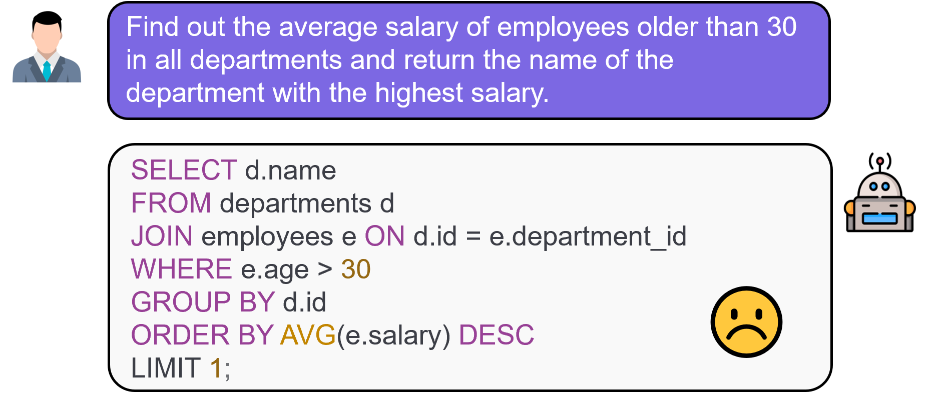
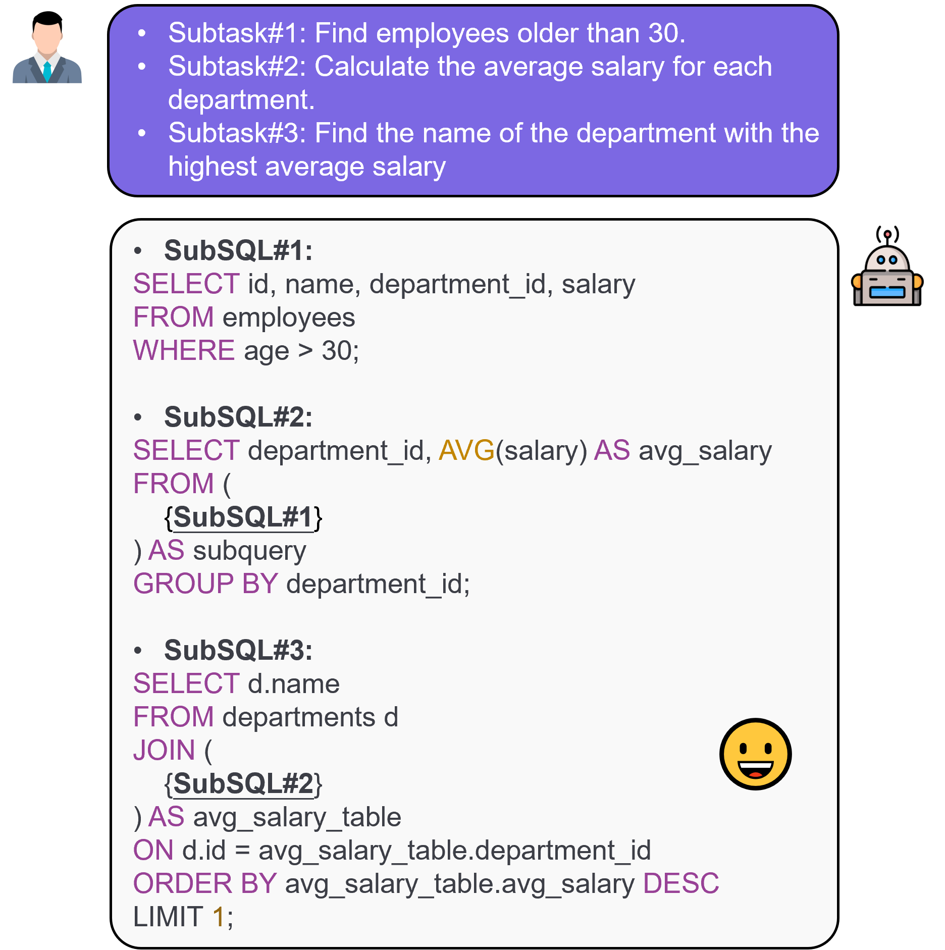
Figure 1: (a) illustrates the LLM directly solving a complex NL2SQL task, resulting in an incorrect output. (b) shows the LLM solving multiple decomposed simple NL2SQL subtasks from the same task in (a), resulting in a correct output.. a — LLM on complex NL2SQL task., b — LLM on multiple simple NL2SQL subtasks.
![Figure 2: The abstract syntax tree (AST) of the given case in Fig. 1. Each simple NL2SQL subtask in Fig. 1 corresponds to a subtree within the AST. Clause nodes, operator nodes and operand nodes were defined in Sec. [ssec:AST].](/article/2504.02327/figures/AST-case.png "fig:")

1 Introduction↩︎
Natural Language to SQL (NL2SQL) [1] is a task that aims to automatically translate natural language queries into executable SQL statements. This task has attracted considerable attention due to its potential to democratize database access, enabling users without SQL expertise to query and interact with databases using natural language. The accurate conversion of natural language into SQL queries is critical for a wide range of applications, including business intelligence, data analysis, and question-answering systems.
Recently, large language models (LLMs), such as OpenAI’s GPT-4, have achieved state-of-the-art performance on NL2SQL benchmark datasets, including Spider [2] and BIRD [3]. These models have demonstrated significant potential in bridging the gap between natural language and structured database queries. However, existing efforts predominantly rely on closed-source LLMs, such as GPT-4 [4]–[6] and Gemini [7], which heavily depend on prompt engineering techniques [8] to achieve optimal results. The reliance on closed-source models introduces several challenges, including concerns about openness, privacy, and computational costs. In contrast, recent efforts to utilize open-source LLMs [9], [10] have faced substantial performance gaps [4], [6], [11] compared to their closed-source counterparts.
To bridge this performance disparity, prior research has explored strategies such as pre-training [12] and post-training [11] to equip LLMs with domain-specific knowledge. However, NL2SQL tasks present unique challenges. Natural language queries often contain multiple objectives, which may be explicit (directly corresponding to query results) or implicit (e.g., conditions for filtering results) and are not always directly mappable to the database schema. These characteristics make it exceedingly difficult for LLMs to effectively solve complex NL2SQL tasks in a single step.
A promising approach to address this complexity is task decomposition, which involves breaking down a complex NL2SQL query into simpler subtasks, as illustrated in Fig.1. Recent research[8] has demonstrated that multi-step reasoning methods, such as the “Let’s think step by step” strategy [13], can significantly enhance LLM performance on natural language processing (NLP) tasks through task decomposition.
Building on this idea, we propose a task decomposition framework to tackle complex NL2SQL queries by dividing them into multiple, simpler subtasks. Preliminary experiments (as shown in Fig. 3) validate this approach: when subtasks are manually provided to the LLM, performance improves significantly (30.4%\(\uparrow\)), underscoring the potential of task decomposition for enhancing NL2SQL performance. However, when the LLM itself is tasked with decomposing complex queries, performance gains are marginal (3.4%\(\uparrow\)), highlighting the need to improve LLMs’ task decomposition capabilities for NL2SQL.
Inspired by recent advancements [14], [15] that leverage reinforcement learning
(RL) [16] to enhance LLM reasoning in multi-step tasks, we propose Learning NL2SQL with AST-guided Task Decomposition
(LearNAT). This novel RL-based algorithm is designed to improve LLMs’ task decomposition capabilities, thereby enhancing their ability to parse complex SQL queries. Specifically, LearNAT introduces methodologies for the three
foundational RL processes—training data synthesis, model training, and inference—by incorporating the following innovations:

Technical challenges and Solutions.
Decomposition Synthesis Procedure: This component employs a search-based strategy, such as Monte Carlo Tree Search (MCTS), to generate subtasks for NL2SQL decomposition. Existing LLM-MCTS hybrid methods rely on heuristic evaluation strategies, where the LLM itself assesses node rewards to guide the search. However, even advanced models like GPT-4 achieve only 46.35% accuracy on benchmarks such as BIRD, limiting the reliability of such self-evaluation methods. Additionally, the vast search space inherent in text-based MCTS leads to inefficiencies and computational overhead. To address these challenges, we leverage abstract syntax trees (ASTs) to guide the search and implement pruning strategies, significantly improving search efficiency and the success rate of generating valid decompositions.
Margin-Aware Reinforcement Learning: This component enhances LLMs’ decomposition capabilities by adopting reinforcement learning techniques, such as Direct Preference Optimization (DPO) [17]. Standard DPO algorithms, however, struggle with fine-grained supervision in multi-step reasoning tasks, as they treat all correct and incorrect steps equivalently. To overcome this limitation, we introduce an AST-based margin-aware DPO framework that distinguishes between varying levels of correctness in steps, enabling more precise optimization.
Adaptive Demonstration Reasoning: Prior studies [8] have shown that incorporating demonstrations into prompts can significantly improve LLM performance through in-context learning. Building on this insight, we develop an adaptive demonstration selection mechanism that dynamically identifies and injects the most relevant demonstrations into prompts, further refining task decomposition capabilities.
Our contributions can be summarized as follows:
We address the critical challenge of enabling LLMs to understand users’ high-level semantics and map them to database schemas for complex NL2SQL problems. To this end, we propose
LearNAT, a novel framework that improves LLM performance on NL2SQL tasks by leveraging task decomposition and reinforcement learning.We introduce the Decomposition Synthesis Procedure, which utilizes AST-guided search and pruning to efficiently generate subtasks, and Margin-Aware Reinforcement Learning, which enables fine-grained preference learning for multi-step reasoning.
Through extensive experiments on two NL2SQL benchmark datasets, we demonstrate that
LearNATsignificantly outperforms existing methods, achieving GPT-4-level performance with a 7B parameter model. These results highlight the efficacy of task decomposition strategies in addressing the challenges of complex NL2SQL tasks.
2 Related Work↩︎
2.1 NL2SQL Parsing Based on LLMs↩︎
Prompt Engineering. Prompt engineering [18] aims to guide model outputs towards desired results through carefully designed input prompts and can be applied to both open-source and proprietary models. In the NL2SQL domain, prompt engineering serves as a crucial technique for enhancing the performance of LLMs [1], [19]. Several studies [4], [5], [7], [20]–[22] have explored different prompt engineering strategies to enhance NL2SQL performance. The most relevant works are DIN-SQL [23] and MAC-SQL [6], which employ zero-shot prompting (Let’s think step by step) or few-shot prompting (e.g., using a small set of demonstrations) to help LLMs decompose complex NL2SQL tasks. While these methods have achieved significant success on publicly available NL2SQL benchmarks, open-source models, constrained by smaller parameter sizes and limited pretraining knowledge, exhibit substantially weaker performance in task decomposition compared to closed-source models [24].
Model Fine-tuning. Model fine-tuning [25] adapts pre-trained LLMs to specific tasks by adjusting model parameters through additional training. While promising for NL2SQL, this approach is limited to open-source models with accessible parameters. Due to the performance gap between open-source and closed-source models, existing research has primarily focused on prompt engineering, with relatively few studies [11], [12], [26]–[28] dedicated to fine-tuning open-source models. Despite their empirical success, these studies focus solely on learning the target SQL queries while neglecting the reasoning process involved in parsing complex SQL structures. This results in mere memorization of outcomes rather than fostering a deep understanding of the underlying problems.
2.2 Enhancing Reasoning with RL↩︎
Search-Guided Reasoning in LLMs. Recent research efforts [15], [29], [30] aiming at advancing the reasoning capabilities of LLMs have increasingly incorporated Monte Carlo Tree Search to generate trajectories for model training, yielding significant improvements in reasoning performance. MCTS effectively balances exploration and exploitation, leveraging its forward-looking strategy to provide high-quality, step-level guidance. Despite these successes, MCTS-driven methods still face several challenges, such as the vast search space inherent to language models and the difficulty of quantifying node rewards. Existing research in the mathematical domain primarily relies on self-evaluation or training external evaluation models based on labeled data. In the NL2SQL domain, we introduce a novel approach that leverages abstract syntax trees to quantify node rewards, effectively guiding the model to prioritize the exploration of the most valuable nodes.
Direct Preference Optimization (DPO) Algorithms. Among various reinforcement learning algorithms, Direct Preference Optimization (DPO) [17] has gained popularity due to its simplicity. DPO relies on instance-level preference signals for model optimization. However, it faces challenges in handling multi-step reasoning tasks, as it struggles to rectify specific errors that arise during the reasoning process [31], [32]. Additionally, relying on model-generated positive samples can reinforce misleading correlations that stem from flawed intermediate steps, thereby weakening generalization [33]. To address these challenges, recent research has introduced step-level DPO [33], [34], which offers more granular error identification and thus improves reasoning accuracy. However, the naive DPO algorithm struggles to capture fine-grained, step-level supervisory signals in multi-step preference learning. This uniform treatment of all correct and incorrect steps significantly limits the model’s potential for optimization.
3 Preliminaries↩︎
Natural Language to SQL (NL2SQL). The goal of the NL2SQL task is to translate a natural language (NL) question \(Q\) into corresponding SQL query \(Y\), based on a database schema \(S\). In more complex scenarios, such as those presented by BIRD [3], interpreting NL questions or understanding database values may require incorporating external knowledge, denoted by \(\mathcal{K}\). The prevailing approach to the NL2SQL task adopts a cross-domain framework to assess a model’s generalization ability by keeping the training, development, and test sets distinct.
Abstract Syntax Trees (AST). An Abstract Syntax Tree (AST) is a structured, hierarchical representation of an SQL query, where each element of the query is captured as a node and the relationships between these elements are encoded as edges. This tree-based structure abstracts away from the linear textual representation of SQL, focusing instead on its grammatical structure and logical organization.
Formally, the AST of an SQL query \(Y\) can be defined as a directed acyclic graph (DAG) \(\mathcal{AT}(Y) = (\mathcal{N}, \mathcal{E})\), where \(\mathcal{N}\) is the set of nodes, each representing a syntactic component of the SQL query. Specifically, every node \(n \in \mathcal{N}\) corresponds to a clause, operator, or operand. We categorize the nodes as follows:
Clause Nodes (\(n_c \in \mathcal{N}_c\)): Represent core SQL clauses, such as
SELECT,FROM,WHERE,GROUP BY, andORDER BY.Operator Nodes (\(n_o \in \mathcal{N}_o\)): Represent logical or arithmetic operations, such as
AND,OR, \(=\), \(>\), and<.Operand Nodes (\(n_v \in \mathcal{N}_v\)): Represent terminal elements like table names, column names, literals, or values from the database schema.
\(\mathcal{E} \subseteq \mathcal{N} \times \mathcal{N}\) is the set of edges, where each directed edge \(e = (n_i, n_j) \in \mathcal{E}\) captures a syntactic dependency from a parent node \(n_i\) to a child node \(n_j\). These edges reflect the hierarchical structure of the query, where high-level clauses dominate subcomponents or conditions.
The root node of \(\mathcal{AT}(Y)\) corresponds to the main clause of the query, typically the SELECT clause. From the root, child nodes represent subsequent clauses or expressions, forming a hierarchical
decomposition of the SQL query. For example, a WHERE clause node may have child nodes corresponding to individual conditions, which in turn may contain operators and operands as descendants.
| Symbol | Description |
|---|---|
| Natural Language to SQL (NL2SQL) | |
| \(Q\) | Natural language (NL) question |
| \(Y\) | Corresponding SQL query |
| \(\mathcal{DB}\) | Database schema |
| \(\mathcal{K}\) | External knowledge |
| Abstract Syntax Trees (AST) | |
| \(\mathcal{AT}(Y) = (\mathcal{N}, \mathcal{E})\) | |
| of SQL query \(Y\) | |
| \(\mathcal{N}\) | Set of nodes in AST |
| \(\mathcal{E} \subseteq \mathcal{N} \times \mathcal{N}\) | Set of edges in AST |
| \(n_c \in \mathcal{N}_c\) | Clause Nodes |
| \(n_o \in \mathcal{N}_o\) | Operator Nodes |
| \(n_v \in \mathcal{N}_v\) | Operand Nodes |
| Monte Carlo Tree Search (MCTS) | |
| \(\mathcal{T} = (\mathcal{S}, \mathcal{A}, \mathcal{M})\) | MCTS search tree |
| \(\mathcal{S}\) | Set of states or nodes in the search space |
| \(\mathcal{A}(s)\) | Set of actions available at state \(s\) |
| \(\mathcal{M} \subseteq \mathcal{S} \times \mathcal{S}\) | Set of edges |
| \(s_0\) | Root node state |
| \(a^*\) | Optimal action based on UCT criterion |
| \(Q(s, a)\) | Estimated reward for taking action \(a\) from state \(s\) |
| \(N(s)\) | Visit count of node \(s\) |
| \(c\) | |
| trade-off | |
| Direct Preference Optimization (DPO) | |
| \(x\) | Prompt |
| \(y_w\) | Preferred response |
| \(y_l\) | Dispreferred response |
| \(p^{*}_{\mathcal{D}}\) | Probability of preference |
| \(\pi_{\theta}\) | Policy model |
| \(\pi_{ref}\) | Reference model |
| \(\beta\) | Parameter that regulates the KL divergence |
Monte Carlo Tree Search (MCTS). Monte Carlo Tree Search (MCTS) is a heuristic search algorithm used for decision-making in large and complex search spaces. It combines tree-based search with stochastic sampling to balance exploration and exploitation, making it particularly effective for problems with vast or unknown state spaces.
Formally, MCTS operates on a search tree \(\mathcal{T} = (\mathcal{S}, \mathcal{A}, \mathcal{M})\), where:
\(\mathcal{S}\) is the set of states or nodes in the search space. Each node \(s \in \mathcal{S}\) represents a specific configuration of the environment, such as a partially completed plan or a subproblem in a reasoning task.
\(\mathcal{A}(s)\) denotes the set of actions available at state \(s\). Each action leads to a child state \(s'\), expanding the search tree.
\(\mathcal{M} \subseteq \mathcal{S} \times \mathcal{S}\) represents the set of edges, where each edge corresponds to a transition between states through an action.
The MCTS algorithm proceeds iteratively through four phases:
Selection: Starting from the root node \(s_0\), the algorithm recursively selects child nodes based on a selection policy, typically using the Upper Confidence Bound for Trees (UCT) criterion: \[\label{equ:UCT} a^* = \arg\max_{a \in \mathcal{A}(s)} \left( Q(s, a) + c \cdot \sqrt{\frac{\log N(s)}{N(s, a)}} \right),\tag{1}\] where \(Q(s, a)\) is the estimated reward for taking action \(a\) from state \(s\), \(N(s)\) is the visit count of node \(s\), \(N(s, a)\) is the visit count of action \(a\) from \(s\), and \(c\) is a constant that controls the exploration-exploitation trade-off.
Expansion: If the selected node is not terminal and has unvisited child nodes, the algorithm expands the tree by adding a new child node corresponding to a valid action from the current state.
Simulation (Rollout): From the newly expanded node, a simulation is conducted by selecting actions—often at random or based on a heuristic policy—until reaching a terminal state. The outcome of this simulation provides a reward signal, used to estimate the reward of the node.
Backpropagation: The reward obtained from the simulation is propagated back through the visited nodes, updating the reward estimations \(Q(s, a)\) and visit counts \(N(s, a)\) along the path from the expanded node to the root.
The output of MCTS is a policy that selects the action with the highest visit count from the root node: \[\pi(s_0) = \arg\max_{a \in \mathcal{A}(s_0)} N(s_0, a).\]
Direct Preference Optimization (DPO). Reinforcement Learning from Human Feedback (RLHF) [16] is an effective strategy for aligning LLMs with human preference, enhancing robustness, reliability, and safety [35]. It relies on the Bradley-Terry (BT) model [36] to define preference probability based on some reward function. Given a prompt \(x\) and two responses—\(y_w\) (preferred) and \(y_l\) (dispreferred)—the probability of preference can be expressed as:
\[p^{*}_{\mathcal{D}}\left(y_{w} \succ y_{l} \mid x\right) = \sigma\left( r^{*}(x, y_{w}) - r^{*}(x, y_{l}) \right),\]
where \(\sigma(x) = \frac{1}{1+\exp(-x)}\) is the sigmoid function and \(r^*\) represents a latent reward model. RLHF optimizes the policy model \(\pi_{\theta}\) with a Kullback-Leibler (KL) constraint to limit deviation from a reference model \(\pi_{ref}\):
\[\max \mathbb{E}_{x \sim \mathcal{D}, y \sim \pi_{\theta}(y \mid x)} [ r^*(x, y) ] - \beta \mathbb{D}_{KL} [ \pi_{\theta}(y \mid x) \| \pi_{ref}(y \mid x) ].\]
Here, \(\beta\) regulates the KL divergence to prevent reward hacking [37]. While effective, RLHF requires careful hyperparameter tuning and involves complex reward modeling and policy training.
To simplify this process, Direct Preference Optimization (DPO) [17] was introduced, eliminating the need for an explicit reward model. Instead, DPO directly optimizes the policy using paired preference data. Given a prompt \(x\) with responses \((y_w, y_l)\), the DPO objective maximizes the likelihood of the preferred response while minimizing that of the dispreferred one:
\[\begin{align} \label{equ:DPO} \mathcal{L}_{\mathrm{DPO}}(\pi_{\theta}; \pi_{\mathrm{ref}}) &= -\mathbb{E}_{(x,y_w,y_l)\sim\mathcal{D}} \notag \left[ \log \sigma \left( \hat{r}_\theta(x, y_w) - \hat{r}_\theta(x, y_l) \right) \right] \\ \hat{r}_\theta(x, y) &= \beta \log \frac{ \pi_{\theta}(y \mid x) }{ \pi_{\mathrm{ref}}(y \mid x) }. \end{align}\tag{2}\]
This formulation treats \(\hat{r}_\theta(x, y)\) as an “implicit reward” [17], allowing for direct alignment with human preference while bypassing the need for complex reward modeling and simplifying the overall training process.
4 Methodology↩︎
In this section, we present the methodology of LearNAT. First, LearNAT employs the Decomposition Synthesis Procedure for generating training data in offline reinforcement learning. Then, it utilizes Margin-aware
Reinforcement Learning for model fine-tuning. Finally, it adopts Adaptive Demonstration Reasoning for NL2SQL with task decomposition.
4.1 Decomposition Synthesis Procedure↩︎
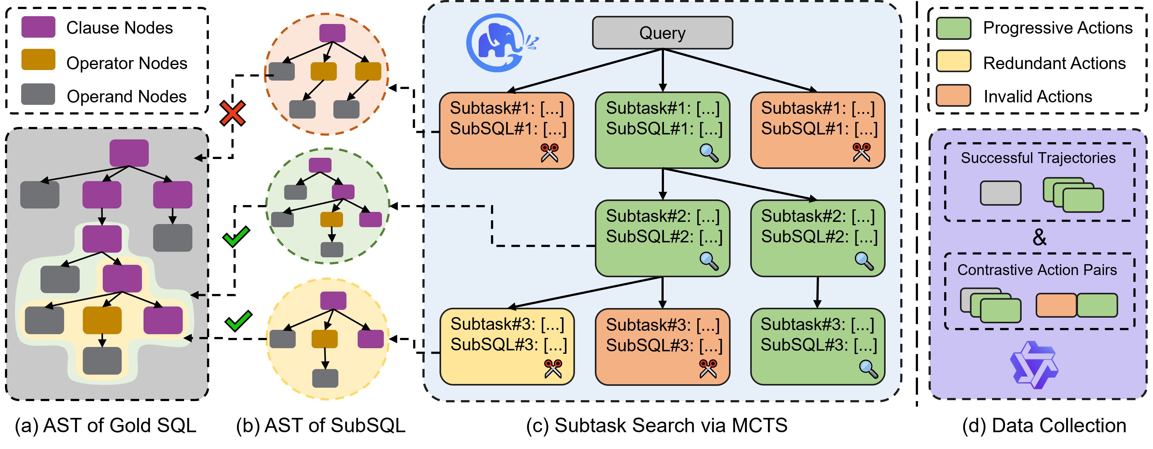
LearNAT employs the Decomposition Synthesis Procedure for generating training data. The framework of the Decomposition Synthesis Procedure is shown in Fig. 5. Given a
natural language query \(Q\), external knowledge \(K\), database schema \(\mathcal{DB}\), and target SQL query \(Y\),
Decomposition Synthesis Procedure aims to decompose complex NL2SQL tasks into a series of simpler subtask queries, which can be easily translated into corresponding SQL statements. The decomposition process is guided by MCTS and AST-based
evaluation, ensuring both the correctness and effectiveness of the generated subtasks.
Problem Formulation Let \(\{q_1, q_2, \cdots, q_n\}\) denote a sequence of subtask queries, where \(n\) represents the number of subtasks and each \(q_i\) represents a natural language query that captures a component of the original query \(Q\). For each subtask query \(q_i\), Decomposition Synthesis Procedure generates a corresponding SQL query \(y_i\). The objective is to find a sequence of subtask queries such that their corresponding SQL queries collectively construct the target SQL query \(Y\).
MCTS-based Decomposition Decomposition Synthesis Procedure formulates the decomposition process as a tree search problem, and performs next-step prediction as action \(a\) in each state \(s\). In the Monte Carlo Tree, the root node represents the original query \(Q\), each non-root node represents the state of executing the next subtask, and each path from root node to a leaf node represents a decomposition sequence.
At each state in MCTS, the Decomposition Synthesis Procedure employs an LLM to generate the next subtask \(q_i\) and sub-SQL \(y_i\). Formally, each state \(s_i = \{q_i, y_i, \mathcal{AT}(y_i), \mathcal{AT}_{\text{sum}}(y_i), \mathcal{R}(s_i)\}\), where \(\mathcal{AT}(y_i)\) is the AST of \(y_i\), \(\mathcal{AT}_{\text{sum}}(y_i)\) is the merged AST summarizing all nodes from root to node \(s_i\) in MCTS, and \(\mathcal{R}(s_i)\) is the reward estimation of \(s_i\). The \(\mathcal{AT}_{\text{sum}}(y_i)\) is mathematically defined as follows: \[\mathcal{AT}_{\text{sum}}(y_i) = (\mathcal{N}_{\text{sum}}, \mathcal{E}_{\text{sum}}),\] \[\mathcal{N}_{\text{sum}} = \bigcup_{j=1}^i \mathcal{N}(\mathcal{AT}(y_j)), \mathcal{E}_{\text{sum}} = \bigcup_{j=1}^i \mathcal{E}(\mathcal{AT}(y_j)).\]
Node Classification Decomposition Synthesis Procedure classify actions into three categories based on their AST properties:
Progressive Actions: Actions where \(\mathcal{AT}(y_i)\) is a subtree of \(\mathcal{AT}(Y)\) and \(\mathcal{AT}(y_i)\) is not a subtree of \(\mathcal{AT}_{\text{sum}}(y_{\text{parent}(i)})\). These actions contribute new information toward the target SQL. For two ASTs \(\mathcal{AT}_1 = (\mathcal{N}_1, \mathcal{E}_1)\) and \(\mathcal{AT}_2 = (\mathcal{N}_2, \mathcal{E}_2)\), We define the subtree relationship as follows: \[\text{isSubtree}(\mathcal{AT}_1, \mathcal{AT}_2) = \begin{cases} 1, & \text{if } \mathcal{N}_1 \subseteq \mathcal{N}_2 \text{ and } \mathcal{E}_1 \subseteq \mathcal{E}_2 \\ 0, & \text{otherwise} \end{cases}.\]
Redundant Actions: Actions where \(\mathcal{AT}(y_i)\) is a subtree of \(\mathcal{AT}(Y)\) but is also a subtree of \(\mathcal{AT}_{\text{sum}}(y_{\text{parent}(i)})\). These nodes provide no additional reward to the decomposition.
Invalid Actions: Nodes where \(\mathcal{AT}(y_i)\) is not a subtree of \(\mathcal{AT}(Y)\). These nodes represent incorrect decompositions.
Prune Strategy In traditional MCTS, since the typical scenario involves robotic task execution, \(\mathcal{A}(s)\) is generally defined as a finite action set, such as pick up,
put down, etc. However, in the application of LLMs, \(\mathcal{A}(s)\) is usually an infinite action set. This is because LLMs generate actions in the form of text, meaning that even the same subSQL can be
expressed as multiple different subtask (action) variations. To reduce the search space of MCTS and improve search efficiency, Decomposition Synthesis Procedure adopts a pruning strategy.
Specifically, since the subtask sequence collected by the Decomposition Synthesis Procedure corresponds to the action sequence along the path from the root node to a leaf node in MCTS, redundant actions and invalid actions along the path do not need to be included in the subtask list. Therefore, for states containing redundant or invalid actions, the Decomposition Synthesis Procedure terminates further action searches to perform pruning.
Reward Estimation In MCTS, it is necessary to estimate \(Q(s, a)\) for each state to provide state rewards, thereby guiding the direction of subsequent searches. In general mathematical domains, existing works typically employ either LLM-based self-evaluation or an additional reward model trained for state reward estimation. In this work, the Decomposition Synthesis Procedure further leverages information from the AST and designs a rule-based approach to evaluate the state reward.
Since states with redundant actions and invalid actions are pruned, to improve efficiency, reward estimation is only performed for states with progressive actions. Specifically, Decomposition Synthesis Procedure estimates the reward of the current state based on the similarity between \(\mathcal{AT}(Y)\) and \(\mathcal{AT}_{\text{sum}}(y_i)\) at the current state.
\[\mathcal{R}(s_i) = \text{sim}(\mathcal{AT}_{\text{sum}}(y_i), \mathcal{AT}(Y)),\]
where \(\text{sim}(\cdot,\cdot)\) denotes the AST similarity measure.
Decomposition Synthesis Procedure defines two types of AST similarity, including node-level similarity \(\text{sim}_{\text{node}}\) and structural similarity \(\text{sim}_{\text{struct}}\).
Node-level Similarity (\(\text{sim}_{\text{node}}\)) The node-level similarity considers different types of nodes separately:
\[\label{equ:node-sim} \text{sim}_{\text{node}}(\mathcal{AT}_1, \mathcal{AT}_2) = \sum_{t \in \{c,o,v\}} w_t \cdot \text{sim}_t(\mathcal{AT}_1, \mathcal{AT}_2),\tag{3}\]
where \(w_t\) are weights for each node type with \(\sum_{t} w_t = 1\) and \(t \in \{c,o,v\}\) represents clause nodes, operator nodes, and operand nodes, respectively.
For each node type:
\[\text{sim}_t(\mathcal{AT}_1, \mathcal{AT}_2) = \frac{|\mathcal{N}_t(\mathcal{AT}_1) \cap \mathcal{N}_t(\mathcal{AT}_2)|}{|\mathcal{N}_t(\mathcal{AT}_1) \cup \mathcal{N}_t(\mathcal{AT}_2)|},\]
where \(\mathcal{N}_t(\mathcal{AT}_i)\) is the set of nodes of type \(t\) in AST \(\mathcal{AT}_i\).
Structural Similarity (\(\text{sim}_{\text{struct}}\)) Decomposition Synthesis Procedure define structural similarity using the Tree Edit Distance (TED):
\[\text{sim}_{\text{struct}}(\mathcal{AT}_1, \mathcal{AT}_2) = 1 - \frac{\text{TED}(\mathcal{AT}_1, \mathcal{AT}_2)}{\max(|\mathcal{AT}_1|, |\mathcal{AT}_2|)},\]
where \(\text{TED}(\mathcal{AT}_1, \mathcal{AT}_2)\) is the minimum number of node operations (insertion, deletion, modification) required to transform \(\mathcal{AT}_1\) into \(\mathcal{AT}_2\), and \(|\mathcal{AT}_i|\) is the number of nodes in AST \(\mathcal{AT}_i\).
Finally, Decomposition Synthesis Procedure estimates the reward of the current state as follows:
\[\begin{align} \label{equ:AST-sim} \mathcal{R}(s_i) & = \alpha \cdot \text{sim}_{\text{node}}(\mathcal{AT}_{\text{sum}}(y_i), \mathcal{AT}(Y)) \notag \\ & + \beta \cdot \text{sim}_{\text{struct}}(\mathcal{AT}_{\text{sum}}(y_i), \mathcal{AT}(Y)), \end{align}\tag{4}\]
where \(\alpha\) and \(\beta\) are adjustment factors for the two types of AST similarity, satisfying \(\alpha + \beta = 1\).
Self-improvement Demonstration Decomposition Synthesis Procedure employs few-shot learning to improve the success rate of task decomposition. Few-shot learning is essentially a form of in-context learning, where a few demonstrations are provided to help the LLM understand user intent, mimic the given format, and learn implicit knowledge.
Initially, Decomposition Synthesis Procedure begins with three manually provided task decomposition examples and executes the first round of decomposition. In the \(i\)-th round of decomposition (\(i \geq 2\)), to reduce resource consumption, the procedure only decomposes samples that were not successfully decomposed in the previous \(i-1\) rounds. Specifically, these are cases where, after the entire MCTS execution, the SQL statement produced at any leaf node does not perfectly match the execution result of the Gold SQL.
To improve the success rate of decomposition, Decomposition Synthesis Procedure adopts adaptive demonstrations instead of using the fixed demonstrations from the first round. Specifically, it constructs a demonstration pool, which consists of samples that were successfully decomposed in the previous \(i-1\) rounds. Given a new task decomposition query, the procedure computes the AST similarity between the query and each query in the demonstration pool. It then selects the top-3 most similar queries as demonstrations to be included in the prompt.
Data Collection During the search process, Decomposition Synthesis Procedure collect two types of data for subsequent offline reinforcement learning:
Successful Trajectories: Sequences of \(\{(q_1, y_1), \cdots, (q_n, y_n)\}\) that successfully decompose the target SQL, used for supervised fine-tuning.
Contrastive Action Pairs: Pairs of incorrect action \((q^l_i, y^l_i)\) and their corresponding correct action \((q^w_i, y^w_i)\), used for preference learning.
4.2 Margin-Aware Reinforcement Learning↩︎
LearNAT propose a Margin-aware Reinforcement Learning framework to train the open-source LLM for decomposing complex NL2SQL tasks into manageable subtasks. The framework consists of two phases. First, Margin-aware Reinforcement
Learning fine-tunes the LLM in a supervised manner based on correct decomposition trajectories, enhancing the model’s ability to perform task decomposition and generate the correct output format. Then, Margin-aware Reinforcement Learning
conducts direct preference optimization (DPO) with AST margin on the LLM using contrastive action pairs, suppressing incorrect subtask outputs and achieving finer-grained preference alignment.
Supervised Fine-tuning Given the training data from Decomposition Synthesis Procedure, Margin-aware Reinforcement Learning first performs supervised fine-tuning on successful decomposition trajectories. In a training instance \((Q, \mathcal{DB}, \mathcal{K}, \{(q_1, y_1), \cdots, (q_n, y_n)\})\), \(Q\) is the input query, \(\mathcal{DB}\) is the database schema, \(\mathcal{K}\) is the optional external knowledge, and \(\{(q_1, y_1), \cdots, (q_n, y_n)\}\) is the sequence of correct subtask queries and corresponding subSQLs. Decomposition Synthesis Procedure treats \([Q, \mathcal{DB}, \mathcal{K}]\) as the prompt \(x\) and \(\{(q_1, y_1), \cdots, (q_n, y_n)\}\) as the target response \(t\), so the supervised fine-tuning objective is to minimize the log-likelihood loss:
\[\mathcal{L}_{\text{SFT}} = \mathbb{E}_{(\boldsymbol{x},\boldsymbol{t})}\left[\sum_{i=1}^I\log p_\theta\left(t_i\mid\boldsymbol{t}_{1:i-1},\boldsymbol{x}\right)\right],\]
where \(\theta\) represents the fine-tuned LLM parameters, and \(p_\theta(\boldsymbol{t}\mid\boldsymbol{x})=\prod_{i=1}^Ip_\theta\left(t_i\mid\boldsymbol{t}_{<i},\boldsymbol{x}\right)\) is the conditional probability distribution of target subtask & subSQL sequence \(t\) given prompt \(x\). \(I\) is the sequence length of \(t\), and \(i\) is the auto-aggressive decoding step.
DPO with AST Margin A phenomenon of pessimism suggests that the positive feedback provided by SFT alone cannot prevent LLMs from generating erroneous reasoning pathways. Existing works [17] indicates that, during the SFT phase, as the probability of preferred outputs (correct responses) increases, the probability of dispreferred outputs (incorrect responses) rises as well. Margin-aware Reinforcement Learning employs DPO to suppress incorrect subtask outputs.
Specifically, a training instance takes the form of \((Q, \mathcal{DB}, \mathcal{K}, \\ \{(q_1, y_1), \cdots, (q_{i-1}, y_{i-1})\}, (q^w_i, y^w_i), (q^l_i, y^l_i))\) ,where \(\{(q_1, y_1), \cdots, \\ (q_{i-1}, y_{i-1})\}\) is a verified correct subtask sequence, \((q^w_i, y^w_i)\) and \((q^l_i, y^l_i)\) represent the correct and incorrect subtasks branching from the search tree, respectively. Margin-aware Reinforcement Learning treats \([Q, \mathcal{DB}, \mathcal{K}, \{(q_1, y_1), \cdots, (q_{i-1}, y_{i-1})\}]\) as the prompt \(x\), \((q^w_i, y^w_i)\) as the prefer response, \((q^l_i, y^l_i)\) as the disprefer response, and optimizes \(\theta\) using Eq. 2 .
However, DPO only optimizes the relative likelihood between positive and negative samples. In other words, the model only learns that the positive samples are better than the negative ones, but does not capture how much better the positive samples are compared to the negative ones.
To enable finer-grained preference learning, Margin-aware Reinforcement Learning follows the inspiration of ODPO [38] by incorporating an offset into the DPO loss to measure the reward margin between positive and negative samples. In the original ODPO [38], an additional reward model is trained to estimate rewards for positive and negative samples. Margin-aware Reinforcement Learning extends this approach by directly computing the margin between positive and negative samples using reward estimation based on AST similarity.
Specifically, Margin-aware Reinforcement Learning estimates the reward margin between two samples as follows:
\[\text{margin}((q^w_i, y^w_i), (q^l_i, y^l_i)) = \mathcal{R}(s^w_i) - \mathcal{R}(s^l_i).\]
Finally, the loss of DPO with AST Margin is formulated as follows:
\[\label{equ:MDPO} \begin{align} \mathcal{L}_{\mathrm{MDPO}}(\pi_{\theta}; \pi_{\mathrm{ref}}) =& -\mathbb{E}_{(x,y_w,y_l)\sim\mathcal{D}} \\ & \left[ \log \sigma \left( \hat{r}_\theta(x, y_w) - \hat{r}_\theta(x, y_l) - \triangle_r\right) \right], \end{align}\tag{5}\]
where \(\triangle_r = \text{margin}((q^w_i, y^w_i), (q^l_i, y^l_i))\) is the offset, measuring the reward margin between positive and negative samples.
The AST margin effectively guides the model to learn not only which decomposition steps are preferred, but also how much they are preferred, leading to more nuanced and effective multi-step reasoning capabilities.
4.3 Adaptive Demonstration Reasoning↩︎
Given the LLM trained with Margin-Aware Reinforcement Learning, LearNAT further employs Adaptive Demonstration Reasoning to enhance the LLM’s ability to solve NL2SQL tasks.
Similar to the self-improving demonstrations proposed in Sec. [sssec:Self-improvement-Demonstration], Adaptive Demonstration Reasoning also aims to identify the most helpful demonstrations for solving the current NL2SQL task. However, the key difference is that self-improving demonstrations select demonstrations based on the AST similarity of SQL queries. In contrast, when the LLM infers a new query, its golden SQL is unknown. Therefore, Adaptive Demonstration Reasoning must adopt an alternative approach to measure similarity.
The Adaptive Demonstration Reasoning framework operates in two phases: (1) embedding cache construction and (2) adaptive demonstration retrieval.
Embedding Cache Construction Given a demonstration pool \(\mathcal{D} = \{(Q_i, Y_i)\}_{i=1}^{N}\), where \(Q_i\) represents a natural language query and \(Y_i\) is the corresponding SQL translation, Adaptive Demonstration Reasoning first construct an embedding cache as follows:
\[E(Q) = \theta(Q) \in \mathbb{R}^d,\] where \(E(\cdot)\) denotes the embedding function that maps natural language queries to a \(d\)-dimensional vector space. Adaptive Demonstration Reasoning utilizes the tuned LLM itself to generate these embeddings through a designated embedding endpoint, ensuring the semantic representation aligns with the model’s internal understanding.
This pre-processing step is performed offline to reduce runtime computational overhead during inference.
Adaptive Demonstration Retrieval When a new query \(Q_{\text{new}}\) is presented, Adaptive Demonstration Reasoning employ the following procedure to select the most relevant demonstrations: (1) Compute the embedding of the new query as \(e_{\text{new}} = E(q_{\text{new}})\), (2) Calculate the similarity score between the new query embedding and each cached embedding as follows:
\[\text{sim}(e_{\text{new}}, E(Q_i)) = \frac{e_{\text{new}} \cdot E(q=Q_i)}{||e_{\text{new}}|| \cdot ||E(Q_i)||}.\]
(3) Select the top-\(k\) most similar query-SQL pairs, denoted as
\[\mathcal{T} = \text{TopK}(\{(Q_i, Y_i, \text{sim}(e_{\text{new}}, E(Q_i)))\}_{i=1}^{N}, k).\]
where \(k=3\) in our implementation.
5 Experiments↩︎
5.1 Experimental Setup↩︎
Datasets We use the BIRD-train dataset [3] to synthesize decomposition data for complex NL2SQL tasks within the Decomposition Synthesis
Procedure, which is subsequently employed for Margin-Aware Reinforcement Learning. Then, we utilize BIRD-dev [3] and Spider-dev [2] to evaluate the effectiveness and robustness of LearNAT. Notably, the databases and user questions in the training and test sets differ
completely.
The statistics of BIRD-train, BIRD-dev, and Spider-dev used in this study are shown in Table. 2. Notably, BIRD-train does not categorize queries based on difficulty levels. Additionally, although BIRD-train provides 9,428 data samples, the gold SQL statements for 425 of them cannot be executed by the SQL executor. Therefore, we filter out these samples considering BIRD-train to contain only 9,003 data samples in our subsequent analysis.
| Benchmarks | Queries | |||||||||||||||||||
|---|---|---|---|---|---|---|---|---|---|---|---|---|---|---|---|---|---|---|---|---|
| BIRD-train | ||||||||||||||||||||
| Simple | Moderate | Challenging | Total | |||||||||||||||||
| BIRD-dev | 925 | 465 | 144 | 1,534 | ||||||||||||||||
| Easy | Medium | Hard | Extra Hard | Total | ||||||||||||||||
| Spider-dev | 248 | 446 | 174 | 166 | 1,034 | |||||||||||||||
Evaluation Metrics. Since the SQL expression styles generated by LLMs may differ from the ground truth in NL2SQL benchmarks [39], traditional string-based evaluation metrics, such as Exact Match Accuracy [2], are not suitable for our study. Therefore, following prior works [40]–[42], we adopt the Execution Accuracy (EX) metric, which evaluates the correctness of generated SQL queries by comparing their execution results with those of the corresponding ground-truth queries retrieved from the database.
Baselines. In this experiment, we compare two types of baselines, including 10 prompting-based approaches and 3 fine-tuning-based approaches, as mentioned in Sec. 2.1. The prompting-based methods include C3-SQL [22], ACT-SQL [43], DIN-SQL [23], MetaSQL [44], DAIL-SQL [20], ZeroNL2SQL [42], MAG-SQL [45], MAC-SQL [6], SuperSQL [19] and MCS-SQL [5], while the fine-tuning-based methods include CatSQL [46], SENSE [11] and CodeS [12].
Implementation Details. We employ GLM-4-Plus1 as the primary model for synthesizing decomposition data and fine-tune the model on Qwen2.5-Coder [10], including its 7B, 14B, and 32B versions. We used the PyTorch library to implement all the algorithms based on the open-source HuggingFace transformers [47] and LLaMA-Factory [48]. The experiments are conducted on 8×A100 GPUs. During the SFT stage, we utilize the AdamW optimizer with a learning rate of 2e-5 and a cosine warmup scheduler over three epochs. For DPO training, the Adam optimizer is used with a learning rate of 2e-6, and the \(\beta\) parameter is set to 0.2, in accordance with the original DPO configuration. In Eq. 3 , we assign equal weights to all three nodes, i.e., \(w_c = w_o = w_v = 0.33\). Based on our experimental observations, we set \(\alpha = 0.75\) and \(\beta = 0.25\) in Eq. 4 .
5.2 Results of Decomposition Synthesis Procedure↩︎
5.2.1 Statistical Results↩︎
We evaluated the decomposition performance of the Decomposition Synthesis Procedure on BIRD-train and compared it with several baseline decomposition algorithms, including CoT and naive MCTS. The experimental results are shown in Table. 3.
The results indicate that the Decomposition Synthesis Procedure achieved an 80.00% decomposition success rate, outperforming CoT and naive MCTS by 20.93%\(\uparrow\) and 8.45%\(\uparrow\), respectively. Additionally, it is noteworthy that MCTS generated a large number of invalid searches, leading to excessive token consumption. In contrast, our proposed Decomposition Synthesis Procedure utilizes AST-guided pruning, enabling high-performance and low-cost (56.38%\(\downarrow\)) decomposition synthesis.
We further tested the performance of self-improving demonstrations over multiple rounds. The results show that adaptive demonstrations significantly improve model performance (1.99%\(\uparrow\)). However, this strategy also has inherent limitations. Table. 3 reveals that self-improving demonstrations achieved notable performance gains in the first round (1.32%\(\uparrow\)), but in the subsequent two rounds, the decomposition performance began to diminish (only 0.4%\(\uparrow\) and 0.27%\(\uparrow\)). Therefore, to minimize token consumption, we did not proceed with a fourth round of decomposition.
| Methods | Success Rate | Token Cost |
|---|---|---|
| CoT | 59.07% | 16,735K |
| MCTS | 71.55% | 334,694K |
| + AST Guide | 78.01% | 133,877K |
| + Self-improvement Demonstration | ||
| (1 round) | 79.33% | 137,456K |
| (2 round) | 79.73% | 142,017K |
| (3 round) | 80.00% | 145,977K |
| Spider-dev | BIRD-dev | ||||||||||
|---|---|---|---|---|---|---|---|---|---|---|---|
| 4-8 (r)9-12 | Venue | LLMs | Easy | Medium | Hard | Extra Hard | Total | Simple | Moderate | Challenging | Total |
| Prompting | |||||||||||
| C3-SQL [22] | GPT-4 | 92.7 | 85.2 | 77.6 | 62.0 | 82.0 | 58.9 | 38.5 | 31.9 | 50.2 | |
| ACT-SQL [43] | EMNLP’23 | GPT-4 | 91.1 | 79.4 | 67.8 | 44.0 | 74.5 | ||||
| DIN-SQL [23] | NeruIPS’23 | GPT-4 | 91.1 | 79.8 | 64.9 | 43.4 | 74.2 | 50.7 | |||
| MetaSQL [44] | ICDE’24 | GPT-4 | 91.1 | 74.7 | 64.1 | 36.1 | 69.6 | ||||
| DAIL-SQL [20] | VLDB’24 | GPT-4 | 90.3 | 81.8 | 66.1 | 50.6 | 76.2 | 62.5 | 43.2 | 37.5 | 54.3 |
| GPT-3.5 | 82.0 | ||||||||||
| VLDB’24 | GPT-4 | 84.0 | |||||||||
| MAG-SQL [45] | GPT-4 | 85.3 | 65.9 | 46.2 | 41.0 | 57.6 | |||||
| MAC-SQL [6] | COLING’25 | GPT-4 | 86.7 | 65.7 | 52.7 | 40.3 | 59.4 | ||||
| SuperSQL [19] | VLDB’24 | GPT-4 | 94.4 | 91.3 | 83.3 | 68.7 | 87.0 | 66.9 | 46.5 | 43.8 | 58.5 |
| MCS-SQL [5] | COLING’25 | GPT-4 | 94.0 | 93.5 | 88.5 | 72.9 | 89.5 | 70.4 | 53.1 | 51.4 | 63.4 |
| Fine-tuning | |||||||||||
| CatSQL [46] | VLDB’23 | N/A | 95.8 | 88.3 | 74.7 | 62.7 | 83.7 | ||||
| SENSE [11] | ACL’24 | CodeLLaMA-13B | 95.2 | 88.6 | 75.9 | 60.3 | 83.5 | 55.5 | |||
| CodeS-7B | 94.8 | 91.0 | 75.3 | 66.9 | 85.4 | 64.6 | 46.9 | 40.3 | 57.0 | ||
| CodeS [12] | SIGMOD’24 | CodeS-15B | 95.6 | 90.4 | 78.2 | 61.4 | 84.9 | 65.8 | 48.8 | 42.4 | 58.5 |
| Ours | |||||||||||
| Qwen2.5-Coder-7B | 95.2 | 92.4 | 76.4 | 67.5 | 86.4 | 65.4 | 48.4 | 42.4 | 58.1 | ||
| Qwen2.5-Coder-14B | 95.6 | 91.5 | 80.5 | 68.7 | 86.9 | 68.5 | 51.4 | 45.8 | 61.2 | ||
| Qwen2.5-Coder-32B | 96.4 | 92.4 | 85.1 | 69.3 | 88.4 | 70.7 | 55.5 | 59.0 | 65.0 | ||
5.2.2 Error Case Analysis↩︎
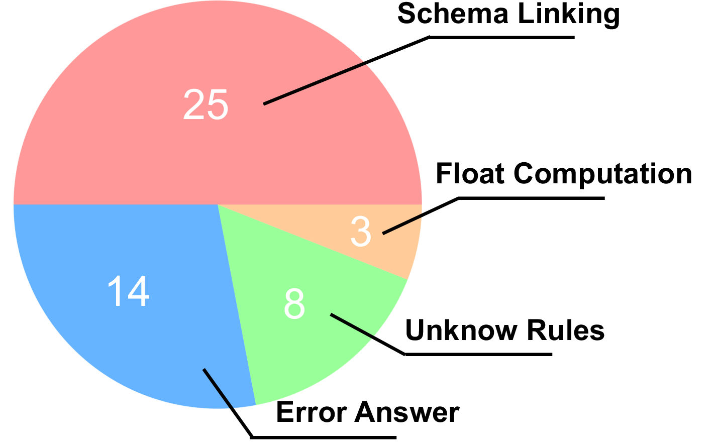
To further investigate the reasons for the failure of the Decomposition Synthesis Procedure in certain cases, we randomly selected 50 unsuccessful cases for error analysis. The error distribution is shown in Fig. 6.
The results indicate that the decomposition failures can be attributed to four distinct types of errors, including schema linking, float computation, unknown rules, and error answer.
We analyze these errors one by one by presenting typical cases for each of the four error attributions.
Case for Schema Linking.
What is the user avatar url for user 41579158? What is the latest movie rated by him / her?
user avatar url refers to user_avatar_image_url; latest movie rated refers to latest rating_date;
[language=SQL, basicstyle=\footnotesize, escapeinside={(@}{@)}]
SELECT T3.user_avatar_image_url, (@\lstul{T3.rating\_date\_utc}@)
FROM movies AS T1
INNER JOIN ratings AS T2 ON T1.movie_id = T2.movie_id
INNER JOIN ratings_users AS T3 ON T3.user_id = T2.user_id
WHERE T3.user_id = 41579158
ORDER BY T3.rating_date_utc DESC
LIMIT 1

[language=SQL, basicstyle=\footnotesize, escapeinside={(@}{@)}]
SELECT user_avatar_image_url, (@\lstul{movie\_id}@) FROM (
SELECT T3.user_avatar_image_url, T3.rating_date_utc FROM (
SELECT T2.user_id, T2.movie_id FROM ratings AS T2
WHERE T2.user_id = 41579158
) AS Sub1
INNER JOIN ratings_users AS T3
ON Sub1.user_id = T3.user_id
WHERE T3.user_id = 41579158
) AS Sub2
ORDER BY rating_date_utc DESC
LIMIT 1;
In this case, the LLM misidentified the column, mapping “the latest movie rated by him/her” to the movie_id column instead of the rating_date_utc column. However, the evidence provided relevant information (although it
did not explicitly specify the corresponding column).
Case for Float Computation.
What is the percentage of the ratings were rated by user who was a subcriber?
user is a subscriber refers to user_subscriber = 1; percentage of ratings = DIVIDE(SUM(user_subscriber = 1), SUM(rating_score)) as percent;
[language=SQL, basicstyle=\footnotesize, escapeinside={(@}{@)}]
SELECT (CAST(SUM(
CASE WHEN user_subscriber = 1 THEN 1 ELSE 0 END
) AS REAL) (@{\lstul{* 100 / COUNT(*)}@)
) FROM ratings
}

[language=SQL, basicstyle=\footnotesize, escapeinside={(@}{@)}]
SELECT (CAST(SUM(
CASE WHEN user_subscriber = 1 THEN 1 ELSE 0 END
) AS REAL) (@\lstul{/ COUNT(*) * 100}@)
) FROM ratings
In this case, the LLM did not strictly follow the Gold SQL in executing multiplication before division but instead generated SQL that performed the operations in the reverse order. Although mathematically equivalent, floating-point arithmetic in SQL can introduce numerical precision variations. Since our evaluation metric is Execution Accuracy, this discrepancy led to an inconsistency in the results. Specifically, the Gold SQL produced an execution result of 21.648420738414252, whereas the Predicted SQL yielded 21.64842073841425.
Case for Unknown Rules.
List all movies with the best rating score. State the movie title and number of Mubi user who loves the movie.
best rating score refers to rating_score = 5; number of Mubi user who loves the movie refers to movie_popularity
[language=SQL, basicstyle=\footnotesize, escapeinside={(@}{@)}]
SELECT (@\keywordul{DISTINCT}@) T2.movie_title, T2.movie_popularity
FROM ratings AS T1 INNER JOIN movies AS T2
ON T1.movie_id = T2.movie_id
WHERE T1.rating_score = 5

[language=SQL, basicstyle=\footnotesize, escapeinside={(@}{@)}]
SELECT T2.movie_title, T2.movie_popularity
FROM ratings AS T1 INNER JOIN movies AS T2
ON T1.movie_id = T2.movie_id
WHERE T1.rating_score = 5
In this case, the Gold SQL performed an additional deduplication step (DISTINCT) on the query results, whereas the Predicted SQL did not. This deduplication is a default user-friendly operation, but it was not explicitly stated in the
query. As a result, the execution results of the Predicted SQL and Gold SQL differed.
| Methods | Spider-dev | BIRD-dev | |||||||
|---|---|---|---|---|---|---|---|---|---|
| 2-6 (r)7-10 | Easy | Medium | Hard | Extra Hard | Total | Simple | Moderate | Challenging | Total |
| 95.2 | 92.4 | 76.4 | 67.5 | 86.4 | 65.4 | 48.4 | 42.4 | 58.1 | |
| Decomposition Synthesis Procedure | |||||||||
| w/o AST Guide | 85.9 | 87.9 | 69.5 | 60.2 | 79.9 | 62.6 | 41.5 | 29.2 | 53.1 |
| Margin-Aware Reinforcement Learning | |||||||||
| w/o SFT | 87.9 | 88.8 | 69.0 | 62.7 | 81.0 | 63.4 | 43.2 | 34.0 | 54.5 |
| w/o MDPO | 87.1 | 88.6 | 70.1 | 62.7 | 80.9 | 62.8 | 42.4 | 31.9 | 53.7 |
| MDPO\(\rightarrow\)DPO | 93.5 | 91.7 | 74.1 | 66.3 | 85.1 | 64.6 | 46.7 | 37.5 | 56.6 |
| Adaptive Demonstration Reasoning | |||||||||
| w/o Demostratioon | 90.7 | 91.5 | 73.6 | 65.1 | 84.0 | 64.2 | 46.0 | 36.8 | 56.1 |
| ADR\(\rightarrow\)RDR | 92.7 | 91.5 | 74.1 | 66.3 | 84.8 | 64.4 | 46.2 | 36.8 | 56.3 |
| \(\rightarrow\)CoT | 87.1 | 85.2 | 75.3 | 56.6 | 79.4 | 57.3 | 37.6 | 36.1 | 49.3 |
| w/o | 82.7 | 84.1 | 71.8 | 54.8 | 77.0 | 56.1 | 34.5 | 33.8 | 47.5 |
Case for Error Answer.
What is the name of the longest movie title? When was it released?
longest movie title refers to MAX(LENGTH(movie_title)); when it was released refers to movie_release_year
[language=SQL, basicstyle=\footnotesize, escapeinside={(@}{@)}]
SELECT movie_title, movie_release_year FROM movies
(@\keywordul{ORDER BY}@)(@\lstul{ LENGTH(movie\_popularity) }@)(@\keywordul{DESC}@)
(@\keywordul{LIMIT}@)(@\lstul{ 1}@)

[language=SQL, basicstyle=\footnotesize, escapeinside={(@}{@)}]
SELECT movie_title, movie_release_year FROM movies
(@\keywordul{WHERE}@)(@\lstul{ LENGTH(movie\_title) = (}@)
    (@\keywordul{SELECT}@)(@\lstul{ MAX(LENGTH(movie\_title)) }@)(@\keywordul{FROM}@)(@\lstul{ movies}@)
(@\lstul{)}@)
Some cases in BIRD-train contain incorrect Gold SQL. For example, in this case, the query requires computing the longest movie, and the evidence explicitly states that the correct computation should be MAX(LENGTH(movie_title)). However, the
Gold SQL incorrectly calculates this by using LENGTH(movie_popularity), which is clearly incorrect. In contrast, the Predicted SQL correctly implements the intended computation. Therefore, the decomposition failure in this case is a false
negative, caused by an error in the Gold SQL.
5.2.3 Comparison with Competitive Literature↩︎
We evaluate LearNAT on Spider-dev and BIRD-dev benchmarks. To further assess LearNAT’s robustness, we fine-tune Qwen2.5-Coder models with 7B, 14B, and 32B parameters. Additionally, we compare LearNAT against recent
competitive baselines from the past two years. The results are presented in Table. 4.
Compared with prompting-based methods, LearNAT—even with only a 7B model—already outperforms most approaches, although these approaches leverage larger-scale models such as GPT-3.5 or GPT-4 as backbone LLMs. MCS-SQL [5] achieves remarkable performance, significantly surpassing other prompting-based methods on both Spider-dev and BIRD-dev, and also outperforming the 7B and 14B versions of
LearNAT. Only when LearNAT scales the model up to 32B can it achieve performance surpassing on BIRD-dev. However, while MCS-SQL delivers impressive results, it relies on multiple interactions with GPT-4. According to the
hyperparameter settings provided in the MCS-SQL manuscript, achieving its reported performance requires more than 60 interactions with GPT-4, making it highly resource-intensive. In contrast, all LearNAT results require only a single
interaction with the LLM.
Compared to fine-tuning-based methods, LearNAT demonstrates a more significant performance advantage. Among the prompting-based approaches mentioned, the most competitive is CodeS [12], therefore we evaluate both the 7B and 15B versions of CodeS. Experimental results show that LearNAT (7B) achieves a 1.0%\(\uparrow\) on Spider-dev and a 1.1%\(\uparrow\) on BIRD-dev over CodeS (7B). Similarly, LearNAT (14B) outperforms CodeS (15B) by a
2.0%\(\uparrow\) on Spider-dev and a 2.7%\(\uparrow\) on Spider-dev. This indicates that
LearNAT maintains a performance advantage across different model sizes.
5.2.4 Ablation Study↩︎
We evaluate the necessity of each component in LearNAT by systematically removing individual components and assessing the model’s performance. We use Qwen2.5-Coder-7B as the backbone LLM and conduct evaluations on Spider-dev and BIRD-dev.
The results are summarized in Table. 5.
First, we present the most naive baseline (w/o LearNAT), which represents the basic performance of Qwen2.5-Coder-7B. Then, we remove the AST-guide, replacing it with naive MCTS for decomposition and using vanilla DPO in reinforcement
learning. The results show an improvement over w/o LearNAT (e.g., 5.6%\(\uparrow\) on BIRD-dev), indicating that decomposition-based RL enhances LLM performance in
complex NL2SQL tasks. However, compared to LearNAT, the model’s performance drops significantly (e.g., 5.0%\(\downarrow\) on BIRD-dev), suggesting that without an
appropriate reward evaluation, performance improvements are limited. LearNAT tightly integrates reward modeling with AST, designing a rule-based reward model that significantly enhances LLM performance.
Next, we remove the SFT stage, leading to a performance drop (e.g., 3.6%\(\downarrow\) on BIRD-dev), indicating that SFT is necessary for initializing the LLM before applying MDPO, aligning with findings from prior work [11]. Similarly, removing MDPO results in a performance decline (e.g., 4.4%\(\downarrow\) on BIRD-dev), showing that SFT alone teaches the LLM to generate correct outputs but fails to suppress incorrect ones [32], which degrades overall model performance. Replacing MDPO with naive DPO further reduces performance, as the lack of margin awareness prevents the LLM from distinguishing critical steps during preference learning, leading to coarse-grained reward estimation and thus suboptimal performance.
We also analyze the importance of few-shot learning by removing demonstrations during inference. The results show that few-shot learning helps the model better follow user intent and learn new knowledge from demonstrations, thereby improving performance. Replacing adaptive demonstration reasoning (ADR) with random demonstration selection (RDR) leads to a performance drop (e.g., 1.8%\(\downarrow\) on BIRD-dev), confirming that adaptive demonstrations allow the model to find more relevant examples, further boosting performance.
Finally, we conduct a simple experiment using naive Qwen2.5-Coder-7B with CoT-based decomposition, where the LLM directly decomposes the NL2SQL task and generates SQL. While this setup improves performance (e.g., 1.8%\(\uparrow\) on BIRD-dev), it is far less effective than LearNAT, highlighting the importance of AST-guide decomposition, reinforcement learning and adaptive
demonstrations.
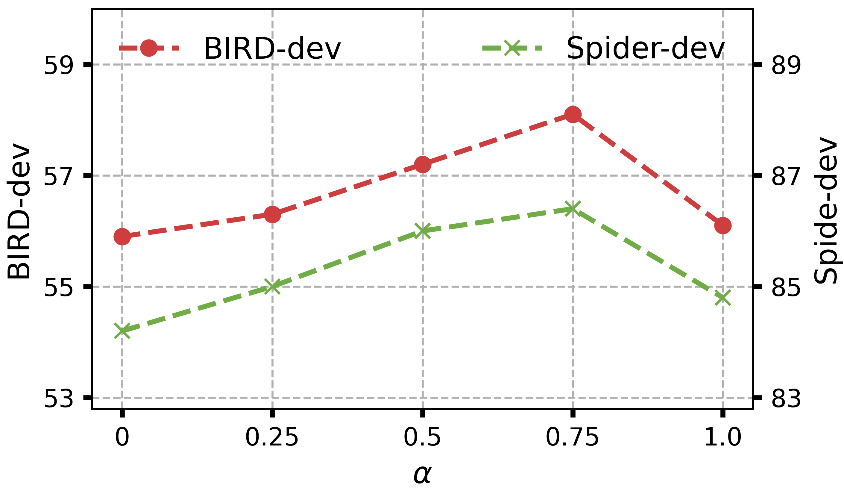
5.2.5 Analysis of AST Similarity↩︎
We evaluate the importance of node similarity and structural similarity in LearNAT by adjusting the weight parameter \(\alpha\) in Eq. 4 . Specifically, we vary \(\alpha\) between 0, 0.25, 0.5, 0.75, and 1.0, while ensuring that \(\alpha + \beta = 1\). When \(\alpha = 0\), the model relies entirely on structural
similarity. When \(\alpha = 1\), the model relies entirely on node similarity.
Experimental results (illustrated in Fig. 7) show that using only node similarity or only structural similarity leads to performance degradation, indicating that both types of similarity contribute to evaluation
quality. A balanced setting (\(\alpha = \beta = 0.5\)) does not achieve optimal performance. LearNAT achieves the best performance when \(0 < \beta < 0.5 < \alpha <
1\), suggesting that node similarity is more effective than structural similarity in AST-based similarity assessment. This highlights that while both node and structural similarity are necessary, node similarity plays a slightly more critical role
in guiding AST-based decomposition and reward estimation.
6 Discussion↩︎
In this section, we investigate two key research questions to further analyze the rationality of LearNAT.
- RQ#1: Is a complex MCTS necessary? Could it be replaced by directly using the subSQLs from the Gold SQL to synthesize subtasks?
The answer is NO. In the early pilot experiments, we designed a more concise approach: starting from the Gold SQL, we extracted a sequence of subSQLs and then used a LLM to translate each subSQL into its corresponding subtask. This initially appeared to be a more effective strategy. However, a critical issue arises—how can we evaluate the correctness of these subtasks? We attempted to directly use a LLM, such as Qwen2-7b-instruct, to determine whether the generated subtasks were correct. However, this approach achieved only 45.4% accuracy, indicating that verifying the correctness of subtasks is not straightforward. The LLM often misjudged due to subtle differences; for example, if the Gold SQL query targeted a user’s name, but the generated subtask query targeted the user’s ID instead, the LLM frequently considered the subtask correct.
In contrast, LearNAT takes the Query as the starting point, generates subtasks for the Query, and verifies them by validating the corresponding subSQLs. Compared to directly verifying the correctness of subtask queries, subSQLs
offer a more structured and stable representation, making validation more straightforward. For instance, LearNAT employs AST-based validation, which enhances the robustness of the verification process.
- RQ#2: Is the evaluation of UCT rewards (see Eq. 1 ) in MCTS necessary? Could it be replaced with a simple depth-first search?
The answer is NO. In MCTS, the role of the UCT is to balance the reward of each state with its exploration count, thereby preventing the search from getting trapped in local optima. If we focus solely on the reward of a state while ignoring its exploration count, MCTS degenerates into a depth-first search strategy, which poses risks in NL2SQL task decomposition for the following reasons:
First, NL2SQL task decomposition is not unique. Even though AST-based subtask evaluation can ensure the correctness of individual subtasks, it sacrifices the diversity of task decomposition. Second, NL2SQL tasks exhibit sequential dependencies, meaning
that changes in the execution order of subtasks can lead to incorrect execution results. However, AST-based subtask evaluation can only guarantee the structural correctness of subtasks but cannot ensure the correctness of their execution order. Therefore,
by penalizing low visitation counts, the UCT reward helps LearNAT escape local optima and enables a broader search, thereby improving the correctness of subtask sequencing.
7 Conclusion and Future Works↩︎
In this work, we propose LearNAT, a novel framework designed to enhance the performance of LLMs on NL2SQL tasks by leveraging task decomposition and reinforcement learning. Our approach addresses a critical challenge in NL2SQL: the
difficulty LLMs face in deeply understanding high-level user semantics and formulating a coherent problem-solving process, particularly for complex queries. To effectively implement the reinforcement learning algorithm, we introduce the AST-guided
Decomposition Synthesis Procedure, which enables efficient search and pruning strategies for task decomposition. Furthermore, we propose Margin-Aware Reinforcement Learning, a fine-grained preference learning mechanism that refines the
decision-making process. We validate the efficacy of LearNAT on two widely-used NL2SQL benchmarks, where experimental results demonstrate significant performance improvements of Qwen2.5-Coder models across three scales, outperforming existing
state-of-the-art NL2SQL methods.
Despite the promising results achieved by LearNAT, certain limitations remain. Specifically, the framework’s mandatory application of task decomposition and SQL parsing to all NL2SQL tasks introduces inefficiencies for simpler queries that
could be directly resolved through “fast tinking”. In such cases, the additional decomposition process imposes unnecessary computational overhead in terms of both reasoning complexity and token usage. As a direction for future work, we plan to explore
adaptive task decomposition techniques that dynamically balance reasoning cost and performance. This adaptive approach would aim to selectively apply task decomposition only when it offers tangible benefits, thereby improving the overall efficiency and
scalability of the framework.