Computing Isomorphisms between Products of Supersingular Elliptic Curves
March 27, 2025
Abstract
The Deligne-Ogus-Shioda theorem guarantees the existence of isomorphisms between products of supersingular elliptic curves over finite fields. In this paper, we present an algorithm for explicitly computing these isomorphisms given the endomorphism rings of the curves. Under GRH, it is proved to run in expected polynomial time. Our approach leverages the Deuring correspondence, enabling us to reformulate computational isogeny problems into algebraic problems in quaternions. Specifically, we reduce the computation of isomorphisms to solving systems of quadratic and linear equations over the integers derived from norm equations. We develop \(\ell\)-adic techniques for solving these equations when we have access to a low discriminant subring. Combining these results leads to the description of an efficient probabilistic Las Vegas algorithm for computing the desired isomorphisms.
1 Introduction↩︎
Algorithms for computing isogenies between elliptic curves have been a vast field of research, leading to the recent development of higher-dimensional techniques in cryptography [1], [2]. In particular, abelian varieties of dimension \(g \geq 2\) isomorphic to a product of supersingular elliptic curves play an important role in this setting [3]–[7]. An important feature of such abelian varieties is that they are all isomorphic over an algebraic closure. Let \(\mathbb{F}_q\) be a finite field of characteristic \(p>0\). An abelian variety defined over \(\mathbb{F}_q\) is superspecial if it is \(\overline{\mathbb{F}_q}\)-isomorphic to a product of supersingular elliptic curves defined over \(\overline{\mathbb{F}_q}\). The Deligne-Ogus-Shioda theorem [8] states that for all \(g>1\), all dimension-\(g\) superspecial abelian varieties defined over \(\mathbb{F}_q\) are \(\overline{\mathbb{F}_q}\)-isomorphic (as unpolarized abelian varieties). The aim of this paper is to investigate computational aspects of this theorem.
Problem 1 (Effective Deligne-Ogus-Shioda problem). Let \(g \geq 2\) be an integer. Given supersingular elliptic curves \(E_1, \dots, E_g\) and \(E_1', \dots, E_g'\) defined over \(\mathbb{F}_q\), compute an \(\overline{\mathbb{F}_q}\)-isomorphism \(E_1\times \cdots \times E_g \to E_1'\times \cdots \times E_g'\).
This appears to be a difficult computational problem. Indeed, computing the endomorphism ring of a supersingular curve is a computational problem which is considered hard, and the security of several cryptographic constructions relies on it [6], [7]. Solving Problem 1 would provide non-trivial information about the endomorphism rings of the curves: From an isomorphism \(E_1\times E_2 \to E_1' \times E_2'\), we can compute four isogenies \(\varphi_{ij}:E_j\to E_i'\), and the composition \(\widehat \varphi_{21} \varphi_{22} \widehat \varphi_{12} \varphi_{11}:E_1 \to E_1\) is in general a non-trivial endomorphism of \(E_1\). In this paper, we study Problem 1 in the context where we have extra information: the endomorphism rings of the elliptic curves are given (see Section 2.2.2 for technical details on the encoding of the endomorphism rings). In this setting, Deuring’s correspondence allows us to translate Problem 1 into a problem about quaternion algebras.
1.1 Contributions↩︎
We focus on the case \(g=2\), which is the base case which serves as a building block for the general case \(g\geq 2\). Therefore our main problem is the computation of an isomorphism \(E_1\times E_2\to E_1'\times E_2'\) between two products of supersingular elliptic curves, assuming that their endomorphisms rings are known. Endomorphism rings are given via an efficient representation of a \(\mathbb{Z}\)-basis together with an explicit isomorphism with a maximal order in the quaternion algebra \(\mathcal{B}_{p,\infty}\). Our main contribution is a polynomial-time algorithm that computes an isomorphism \(E_1\times E_2\to E_1'\times E_2'\) between products of maximal elliptic curves over \(\mathbb{F}_{p^2}\), assuming that we know the endomorphism rings of the curves. This algorithm relies on two main subroutines. The first one describes how to build a two by two matrix of isogenies which is an isomorphism, given its first column. The second one allows us to compute isomorphisms of the form \(E^2 \to E_1' \times E\) when we know a non-scalar low-discriminant endomorphism in \(\mathop{\mathrm{End}}(E)\).
In order to design such algorithms, we need some new computational techniques. We provide a quasi-linear quaternionic method to divide an endomorphism by an isogeny, see Proposition 16. Our main theoretical tool is a necessary and sufficient criterion to decide whether a pair of separable isogenies \(\varphi_{11}:E_1\to E_1'\), \(\varphi_{21}:E_1\to E_2'\) of coprime degrees can appear as the first column of a matrix \((\varphi_{ij})_{i,j\in\{1, 2\}}\) describing an isomorphism \(E_1\times E_2\to E_1'\times E_2'\): this happens when the direct sum of the kernels of \(\varphi_{11}\) and \(\varphi_{21}\) is the kernel of an isogeny \(E_1\to E_2\). This result is formalized in Theorem 25 and is used in our algorithms for both subroutines. In the low-discriminant case, we also use the fact that we can solve efficiently norm equations in low-discriminant imaginary quadratic orders. In both cases, we use Wesolowski’s variant [9] of the KLPT algorithm [10] as an important building block, whose complexity is proved under GRH.
To demonstrate some of the algorithms presented in this paper, we provide a proof-of-concept implementation in the computer algebra software Magma, freely available at [11]. We only compute the quaternionic part of the isomorphisms, meaning that we output four ideals \(\{I_{ij}\}_{1\leq i,j\leq 2}\), which are kernel ideals of four isogenies \(\varphi_{I_{ij}}\), which form a matrix that represents an isomorphism. To recover the isogenies, one can use IdealToIsogeny algorithms, described for example in [6], [12]; see also [13] which provides a general polynomial-time complexity bound for this step.
1.2 Related works↩︎
Superspecial abelian varieties are central objects in the recent developments of isogeny-based cryptography, as they are the main characters of the new high-dimensional techniques, see e.g. [2], [5], [14]. Being able to compute isomorphisms between such objects would be a useful computational tool. In particular, one typical setting is to consider a special curve which has the property that its endomorphism ring contains a low-discriminant imaginary quadratic order. For instance, when \(p\equiv 3\bmod 4\), the endomorphism ring of the elliptic curve \(E_0\) defined over \(\mathbb{F}_{p^2}\) by the equation \(y^2=x^3+x\) contains a subring isomorphic to \(\mathbb{Z}[i]\). Being able to compute an isomorphism between a superspecial abelian variety and \(E_0^g\) would give access to these low-discriminant subrings of endomorphisms. Another application of our work is the representation of some polarized abelian varieties. In particular, the Ibukiyama-Katsura-Oort correspondence shows that superspecial principally polarized abelian surfaces (up to polarized isomorphisms) can be represented via two by two matrices over the quaternions (modulo congruence). Algorithms have been recently developed in [15] to perform efficient computations via this representation. Our algorithms contribute to this toolbox since isomorphisms between products of supersingular elliptic curves can be used to compute the Ibukiyama-Katsura-Oort representation of principally polarized abelian surfaces that are not Jacobians of genus-\(2\) curves.
In the direction of the construction of isomorphisms between products of elliptic curves, one can find in the proof of [16] an explicit construction of an isomorphism between the \(E \times E/(K_1 + K_2)\) and \(E/K_1 \times E/K_2\) for \(K_i\) finite étale subgroups of coprime orders. This result has similarities with our Theorem 25, but it is not general enough for our purposes.
1.3 Organization of the paper↩︎
Section 2 recalls background material. We state our main results in Section 3. In Section 4, we develop computational tools that will be required in the main algorithms. Section 5 is devoted to the computation of isomorphisms between products of supersingular elliptic curves provided that we know their endomorphism rings.
1.4 Acknowledgements↩︎
We thank Benjamin Wesolowski for providing the ideas that led to the general algorithm in Section 5.4. We thank Jean Kieffer and Damien Robert for fruitful discussions, and the Isocrypt people for their interest. We thank Marc Houben for pointing us to [16]. This work received funding from the France 2030 program managed by the French National Research Agency under grant agreements No. ANR-22-PETQ-0008 PQ-TLS and ANR-22-PECY-0010.
2 Background↩︎
For an elliptic curve \(E\) over a field \(k\), we denote by \(\mathop{\mathrm{End}}(E)\) its ring of endomorphisms defined over \(\overline{k}\), the algebraic closure of \(k\). We assume that the characteristic \(p\) of finite fields is greater than \(3\). For \(p=2,3\), the algorithmic questions discussed in this paper are trivial since all supersingular elliptic curves are isomorphic.
Throughout this paper, we use the formalism of group schemes to describe kernels of (non-necessarily separable) isogenies, so that any nonzero isogeny (even if it is purely inseparable) has a non-trivial kernel. We refer to [17] for more details on this formalism. In particular, for an elliptic curve \(E\) defined over \(\overline{\mathbb{F}_p}\), there are bijections between proper left-ideals in \(\mathop{\mathrm{End}}(E)\), finite group subschemes in \(E\), and isogenies with domain \(E\) up to post-composition by isomorphisms. This follows from the fact that all left-ideals in \(\mathop{\mathrm{End}}(E)\) are kernel ideals, see [17] for the cases where \(\mathop{\mathrm{End}}(E)\) has rank \(1\) or \(4\), and [18] for the CM-case. We also use the following convenient notation: given a finite subgroup scheme \(K\) of an elliptic curve \(E\), we let \(E\to E/K\) denote the geometric quotient of \(E\) by \(K\), where \(K\) acts by translation. Therefore, an elliptic curve \(E'\) is isomorphic to \(E/K\) if and only if there exists an isogeny \(E\to E'\) whose kernel is \(K\). We call the map \(E\to E/K\) the canonical isogeny with kernel \(K\).
Elliptic curves over \(\mathbb{F}_{p^2}\) whose number of rational points equals the Hasse-Weil upper bound \((p+1)^2\) are called maximal.
Remark 2. Any supersingular curve \(E\) over a field \(k\) of characteristic \(p>0\) is \(\overline{k}\)-isomorphic to a curve defined over \(\mathbb{F}_{p^2}\), see [19]. Therefore, for computational purposes, it is convenient to consider supersingular curves defined over \(\mathbb{F}_{p^2}\). Moreover any such curve is \(\overline{\mathbb{F}_p}\)-isomorphic to a maximal curve \(E'\) (see [20] and [21]), which has the convenient property that all endomorphisms and isogenies with domain \(E\) are also defined over \(\mathbb{F}_{p^2}\), see [21].
2.1 Deuring correspondence↩︎
We recall key concepts of the Deuring correspondence. For a more comprehensive study of the subject, we refer to [22] and [19].
2.1.1 Quaternion algebras.↩︎
Let \(p\) be a prime. We focus on the (unique up to isomorphism) quaternion algebra \(\mathcal{B}_{p,\infty}\) over \(\mathbb{Q}\) which is ramified at \(p\) and \(\infty\). The algebra \(\mathcal{B}_{p,\infty}\) is non-commutative, and it has dimension \(4\) over \(\mathbb{Q}\). When \(p \equiv 3 \bmod 4\), a \(\mathbb{Q}\)-basis is \(1,i,j,k\), where \(i^2= -1\), \(j^2= -p\) and \(k = i\, j= - j\, i\).
Any element \(\alpha \in \mathcal{B}_{p,\infty}\) can be encoded by coordinates \((\alpha_0, \alpha_1, \alpha_2, \alpha_3) \in \mathbb{Q}^4\), such that \(\alpha = \alpha_0 + \alpha_1 i + \alpha_2 j + \alpha_3 k\). The conjugate of \(\alpha=\alpha_0 + \alpha_1 i+\alpha_2 j +\alpha_3 k\in \mathcal{B}_{p,\infty}\) is \(\overline{\alpha}=\alpha_0 - \alpha_1 i - \alpha_2 j - \alpha_3 k\). Its reduced trace is \(\mathop{\mathrm{Trd}}(\alpha)=\alpha + \overline{\alpha} = 2\alpha_0\) and its reduced norm is \(\mathop{\mathrm{Nrd}}(\alpha)=\alpha \cdot \overline{\alpha} = \alpha_0^2 + \alpha_1^2 + p(\alpha_2^2+\alpha_3^2) \in \mathbb{Q}\). Every nonzero \(\alpha\in\mathcal{B}_{p,\infty}\) is invertible, i.e., there exists a unique \(\beta\in\mathcal{B}_{p,\infty}\) such that \(\alpha\cdot\beta = \beta\cdot\alpha = 1\).
An order in \(\mathcal{B}_{p,\infty}\) is a subring which has rank \(4\) as a \(\mathbb{Z}\)-module. An order is maximal when it is not contained in a strictly larger order. A fractional ideal \(I\) is a rank-\(4\) \(\mathbb{Z}\)-module in \(\mathcal{B}_{p,\infty}\). The left and right orders of \(I\) are defined as: \[\mathcal{O}_{L}(I) = \{ \alpha \in \mathcal{B}_{p,\infty}: \alpha I \subset I \}, \quad \mathcal{O}_{R}(I) = \{ \alpha \in \mathcal{B}_{p,\infty}: I \alpha \subset I \}.\]
When \(I \subset \mathcal{O}_{L}(I)\) (or equivalently \(I \subset \mathcal{O}_{R}(I)\), see [19]), we say that \(I\) is an integral ideal. Integral ideals in maximal orders are actually locally principal [19]. This implies that the completion \(I \otimes \mathbb{Z}_{\ell}\) of an ideal \(I\) in an order \(\mathcal{O}_{}\) at a prime \(\ell\) unramified in \(\mathcal{B}_{p,\infty}\) generates a principal ideal in \(\mathcal{O}_{}\otimes\mathbb{Z}_\ell\cong \mathop{\mathrm{M}}_2(\mathbb{Z}_\ell)\). We study localizations in more details in Section 4.4. Remark that any integral ideal \(I\) is a left-\(\mathcal{O}_{L}(I)\) ideal, and a right-\(\mathcal{O}_{R}(I)\) ideal. In the following we will use basic results and terminology about ideals in quaternion orders and their norms, as exposed in [19]. In particular, the set \(\mathop{\mathrm{Conn}}(\mathcal{O}_{1},\mathcal{O}_{2})\) of connecting ideals between orders \(\mathcal{O}_{1}, \mathcal{O}_{2}\subset \mathcal{B}_{p,\infty}\) is the set of invertible lattices \(I\) such that \(\mathcal{O}_L(I) = \mathcal{O}_{1}\) and \(\mathcal{O}_R(I) = \mathcal{O}_{2}\).
2.1.2 The correspondence.↩︎
Endomorphism rings of supersingular elliptic curves are isomorphic to maximal orders in \(\mathcal{B}_{p,\infty}\). The purpose of Deuring correspondence is to provide a set of tools for representing geometric objects related to supersingular elliptic curves as algebraic objects in \(\mathcal{B}_{p,\infty}\).
Theorem 3. [19] Let \(E\) be a supersingular elliptic curve defined over \(\overline{\mathbb{F}_p}\). Then \(\mathop{\mathrm{End}}(E)\) is isomorphic to a maximal order in \(\mathcal{B}_{p,\infty}\).
Let \(\mathcal{O}\subset\mathcal{B}_{p,\infty}\) be a maximal order isomorphic to the endomorphism ring \(\mathop{\mathrm{End}}(E)\) of a supersingular elliptic curve \(E\) defined over \(\overline{\mathbb{F}_q}\). We will implicitly use the isomorphism \(\mathop{\mathrm{End}}(E) \simeq \mathcal{O}_{}\). There is an anti-equivalence between the category of supersingular elliptic curves over \(\overline{\mathbb{F}_q}\) and the category of invertible left \(\mathcal{O}\)-modules. This anti-equivalence is given explicitly via the contravariant functor \(\mathop{\mathrm{Hom}}(\_, E)\), see [19]. It establishes a dictionary between the geometric world of supersingular elliptic curves and the algebraic world of quaternion orders.
On the one hand, let \(J\) be a left \(\mathop{\mathrm{End}}(E)\)-ideal. It defines a subgroup scheme \(E[J]:= \cap_{\alpha \in J}\ker \alpha\) in \(E\), which is the kernel of an isogeny \(\varphi_J:E \to E/E[J]\), see [19]. If \(\varphi_J\) is separable, then \(E[J]=\{ P \in E(\overline{\mathbb{F}_q}) \mid \forall \alpha \in J, \, \alpha(P)=0 \}\). On the other hand, let \(\varphi: E \to E'\) be an isogeny. Then \(I_\varphi:=\mathop{\mathrm{Hom}}(E',E)\varphi\) is a left \(\mathop{\mathrm{End}}(E)\)-ideal which connects the endomorphism rings of \(E\) and \(E'\simeq E/\ker(\varphi)\), regarded as maximal orders in \(\mathcal{B}_{p,\infty}\) up to conjugation. Moreover, for a left-ideal \(J\subset\mathcal{O}\) and \(\psi:E \to E'\), we have that \(J=I_{\varphi_{J}}\) and \(\psi \cong \varphi_{I_{\psi}}\). In particular we have a bijection between isomorphism classes (i.e., isogenies up to post-composition by isomorphisms) of isogenies from \(E\), and left-ideals \(I\) in \(\mathcal{O}\). See [22] for a summary of the dictionary given by Deuring correspondence.
2.2 Efficient representations of isogenies↩︎
In order to implement the constructions of this work, we have to define what is a good representation of an isogeny. We will use the notion of efficient representation designed in [23], [24].
A representation of an isogeny \(\varphi: E\to E'\) between elliptic curves defined over \(\mathbb{F}_q\), is a set of data that contains the domain, the codomain, the degree \(\deg(\varphi)\), and an algorithm to evaluate \(\varphi\) on any point \(P\in E(\mathbb{F}_{q'})\) for any finite extension \(\mathbb{F}_{q'}/\mathbb{F}_{q}\). In fact, a bound on the degree is sufficient since the degree can then be recovered using [24]. When \(\deg(\varphi)\) is large, we may not be able to use directly accessible \(N\)-torsion for \(N>\deg(\varphi)\); in that case, we can use a powersmooth integer for \(N>\deg(\varphi)\) and a CRT representation as explained in [24]. We say that a representation is efficient if this data enables us to compute the image of a point \(P \in E(\mathbb{F}_{q'})\) in time polynomial in both \(\log(\deg(\varphi))\) and \(\log(q')\). We say that it is compact if the space needed to store the data is polynomial in \(\log(\deg(\varphi))\) and \(\log(q')\). The representation we will use is the ideal representation which relies on the Deuring correspondence.
2.2.1 Ideal representation.↩︎
The core idea of the ideal representation is to represent an isogeny \(\varphi:E \to E'\) via the ideal \(I_\varphi\subset\mathop{\mathrm{End}}(E)\) of all endomorphisms whose kernel contains \(\ker\varphi\), seen as an ideal in a maximal order of \(\mathcal{B}_{p,\infty}\) isomorphic to \(\mathop{\mathrm{End}}(E)\). In order to use this representation, we first need to fix an embedding \(\mathop{\mathrm{End}}(E)\hookrightarrow \mathcal{B}_{p,\infty}\). Although this only encodes the isomorphism class of \(\varphi\), knowing the codomain \(E'\) enables us to determine \(\varphi\) up to post-composition by automorphisms. Consequently, in order to have a full representation of \(\varphi\), we need a bit more data to discriminate these automorphisms. We disregard this subtlety in the present work: the order of \(\mathop{\mathrm{Aut}}(E')\) is at most \(24\), so we can use exhaustive search on \(\mathop{\mathrm{Aut}}(E')\) without harming the complexity. However, in a practical implementation, it might be useful to add some information to remove the ambiguity. Note that if \(j(E') \ne 0,1728\) then \(\mathop{\mathrm{Aut}}(E')=\{\pm 1\}\) [25].
Theorem 4. Given an efficient representation of a \(\mathbb{Z}\)-basis of \(\mathop{\mathrm{End}}(E)\) and its image via an embedding \(\mathop{\mathrm{End}}(E)\hookrightarrow \mathcal{B}_{p,\infty}\), then a \(\mathbb{Z}\)-basis of the ideal \(I_{\varphi}\) provides a compact representation of \(\varphi\). Assuming GRH, this representation is efficient.
For more details, see [24]. We work with \(2\times 2\) matrices whose entries are isogenies, which can be encoded via efficient representations.
Proposition 5. Let \(E_1, E_2, E_1', E_2', E_1'', E_2''\) be elliptic curves defined over \(\mathbb{F}_q\). Let \(M = (\varphi_{ij})_{i,j\in\{1, 2\}}\) (resp. \(N = (\psi_{ij})_{i,j\in\{1, 2\}}\)) be a \(2\times 2\) matrix of isogenies, where \(\varphi_{ij}:E_j\to E_i'\) (resp. \(\psi_{ij}:E_j'\to E_i''\)). Then \(M\) (resp. \(N\)) represents the isogeny \(E_1\times E_2\to E_1'\times E_2'\) (resp. \(E_1'\times E_2'\to E_1''\times E_2''\)) defined as \(\phi_M(P,Q)=(\varphi_{11}(P) + \varphi_{12}(Q), \varphi_{21}(P) + \varphi_{22}(Q))\) (resp. \(\phi_N(P,Q)=(\psi_{11}(P) + \psi_{12}(Q), \psi_{21}(P) + \psi_{22}(Q))\)). Moreover, the matrix product \(N\cdot M = (\sum_{k\in\{1, 2\}} N_{ik}\circ M_{kj})_{i,j\in\{1, 2\}}\) represents an isogeny \(E_1\times E_2\to E_1''\times E_2''\) and efficient representations of the entries of \(N\cdot M\) can be computed in polynomial-time from efficient representations of the entries of \(M\) and \(N\).
Proof. The only thing that we need to prove is that we can compute efficient representations of compositions and sums of isogenies encoded with efficient representations. Algorithms for doing so are described in [24]. ◻
2.2.2 Knowing the endomorphism ring of a curve.↩︎
Throughout this paper, we often say that the endomorphism ring of a supersingular elliptic curve \(E\) is “known” or “given”. By this, we mean that efficient representations of a \(\mathbb{Z}\)-basis \(b_1,\ldots, b_4\) of \(\mathop{\mathrm{End}}(E)\) is given, and that we also have access to elements \(\beta_1,\ldots, \beta_4\in\mathcal{B}_{p,\infty}\) such that the \(\mathbb{Z}\)-module \(\mathcal{O}\) generated by \(\beta_1,\ldots, \beta_4\) in \(\mathcal{B}_{p,\infty}\) is a maximal order and the map \(\mathop{\mathrm{End}}(E)\to\mathcal{O}\) sending \(b_i\) to \(\beta_i\) is a ring isomorphism.
2.3 Superspecial Abelian varieties↩︎
The key theoretical result we rely on is the following statement of existence.
Theorem 6. (Deligne-Ogus-Shioda theorem) [8] Let \(k\) be an algebraically closed field of characteristic \(p > 0\). Let \(E_1, \dots, E_g\) and \(E_1', \dots, E_g'\) be supersingular elliptic curves, where \(g \ge 2\). Then there exists an isomorphism: \(E_1 \times \dots \times E_g \cong E_1' \times \dots \times E_g'.\)
Definition 7. An abelian variety \(\mathcal{A}\) is called superspecial* when it is isomorphic to a product of supersingular elliptic curve.*
In other words, Theorem 6 states that there is only one superspecial abelian variety of each dimension \(g \ge 2\), up to isomorphism. We emphasize that we do not take into account the polarizations of the abelian varieties.
When \(p\equiv 3\bmod 4\), there is a supersingular elliptic curve defined over \(\mathbb{F}_p\) by the equation \(y^2 = x^3 + x\). We denote this special curve by \(E_0\) throughout this paper. A useful feature of \(E_0\) is that \(\mathop{\mathrm{End}}(E_0)\) contains a subring isomorphic to \(\mathbb{Z}[i]\). In the case \(p\equiv 1 \bmod 4\), a similar curve whose endomorphism ring contains a low-discriminant imaginary quadratic subring can be computed efficiently [20]. A direct consequence of Deligne-Ogus-Shioda theorem is that any superspecial variety of dimension \(g\) defined over \(\overline{\mathbb{F}_p}\) is \(\overline{\mathbb{F}_p}\)-isomorphic to \(E_0^g\).
If \(E_1\), \(E_2\), \(E_1'\), \(E_2'\) are supersingular elliptic curves defined over \(\mathbb{F}_{p^2}\), Theorem 6 implies that \(E_1\times E_2\) and \(E_1'\times E_2'\) are \(\overline{\mathbb{F}_p}\)-isomorphic. In fact, when \(E_1, E_2, E_1', E_2'\) are maximal, this isomorphism is defined over \(\mathbb{F}_{p^2}\), see [21].
In this work, we explore the problem of computing explicit isomorphisms between products of supersingular elliptic curves. Moreover, as explained in Remark 2, we can choose maximal models for the supersingular elliptic curves we work with. The goal of this article is thus to find an \(\mathbb{F}_{p^2}\)-isomorphism between the products \(E_1 \times \cdots \times E_g\) and \(E_1' \times \cdots \times E_g'\), where the curves are maximal over \(\mathbb{F}_{p^2}\).
Remark 8. If the supersingular input curves are not maximal, we can start by computing \(\overline{\mathbb{F}_p}\)-isomorphic maximal curves. This can be done efficiently and it does not have any impact on our complexity bounds, see [20].
3 Main Results↩︎
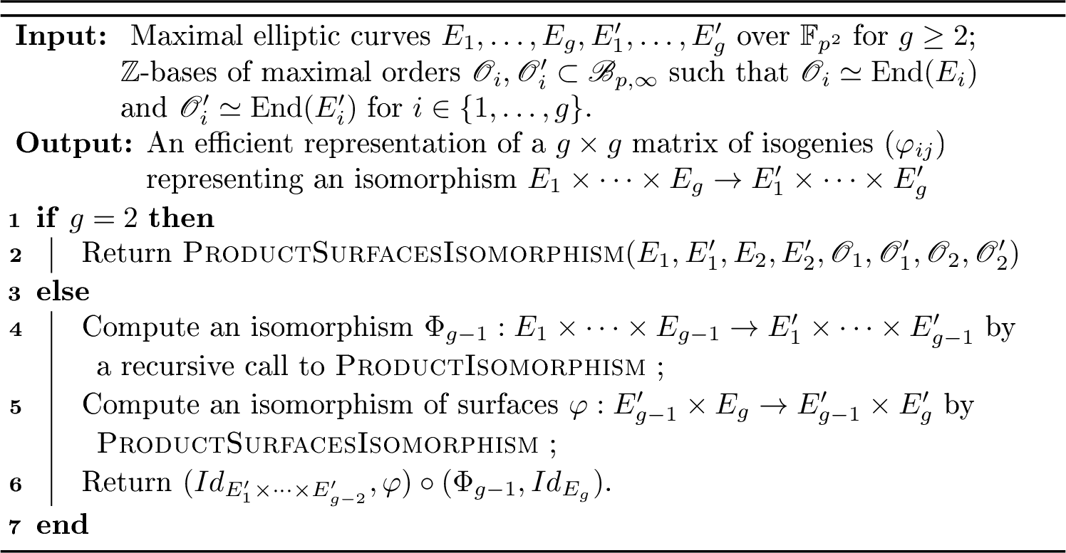
Our main result is Algorithm 1 whose properties are as follows.
Theorem 9. Let \(E_1, \dots, E_g\) and \(E_1', \dots, E_g'\) be maximal elliptic curves over \(\mathbb{F}_{p^2}\) with known endomorphism rings, where \(g \ge 2\). Algorithm 1 is a probabilistic Las Vegas algorithm which computes an \(\mathbb{F}_{p^2}\)-isomorphism of unpolarized abelian varieties: \(E_1 \times \dots \times E_g \cong E_1' \times \dots \times E_g'\). It runs in time linear in \(g\), and polynomial in \(\log(p)\) under GRH.
In fact, the key point is Algorithm 6 which deals with the dimension-2 case, for which we have the following result.
Theorem 10. Let \(E_1,E_2\) and \(E_1', E_2'\) be maximal elliptic curves over \(\mathbb{F}_{p^2}\) with known endomorphism rings. Algorithm 6 is a probabilistic Las Vegas algorithm which computes an \(\mathbb{F}_{p^2}\)-isomorphism of unpolarized abelian surfaces: \(E_1 \times E_2 \cong E_1' \times E_2'\). Assuming GRH, it runs in time polynomial in \(\log(p)\).
The rest of the paper will be dedicated to the proof of Theorem 10. Let us explain how to deduce Theorem 9 from Theorem 10.
Proof of Thm. 9 from Thm. 10. Here we assume that Algorithm 6 is correct. Under this assumption we provide a proof by induction on \(g\) that Algorithm 1 returns the desired isomorphism. By Deligne-Ogus-Shioda theorem, an isomorphism \(E_1\times\dots\times E_g\to E_1'\times\dots\times E_g'\) can be factored as a composition \(E_1\times \dots \times E_g\to E_1'\times \dots\times E_{g-1}'\times E_g \to E_1'\times \dots\times E_g'.\)
This boils down to computing one \((g-1)\)-dimensional isomorphism \(E_1\times\dots\times E_{g-1}\to E_1'\times \dots \times E_{g-1}'\) and one \(2\)-dimensional isomorphism \(E_{g-1}'\times E_g\to E_{g-1}'\times E_g'\). By induction, this proves that computing a \(g\)-dimensional isomorphism can be reduced to computing \(g-1\) isomorphisms in dimension \(2\). Finally, since Algorithm 6 runs in time polynomial in \(\log(p)\) under GRH, the complexity statement follows. ◻
4 Tools↩︎
In this section, we develop tools which will be useful for computing isomorphisms in Section 5. In Section 4.1, we study algorithms for dividing endomorphisms by isogenies. Section 4.2 proves a slight improvement of Kani’s formula for the degree of an isogeny between products of elliptic curves; this is useful for proving that an isogeny is an isomorphism. In Section 4.3, we show how to “transpose” isogenies between products of elliptic curves: we provide an easy way to construct an isogeny \(E_1'\times E_2'\to E_1\times E_2\) from an isogeny \(E_1\times E_2\to E_1'\times E_2'\), while preserving the degree. Finally, in Section 4.4, we design algorithms for finding the generator of the localization of a left-ideal in a maximal order of \(\mathcal{B}_{p,\infty}\).
4.1 Division of principal ideals in quaternion orders↩︎
The first tool that we need is a method for dividing efficiently an endomorphism by an isogeny. More precisely, given an endomorphism \(\phi\in\mathop{\mathrm{End}}(E_1)\), which factors by an isogeny \(f:E_1\to E_2\), we wish to compute an isogeny \(g:E_2\to E_1\) (which is uniquely defined up to composition by automorphisms) such that \(\phi = g\circ f\). A general method when isogenies are given via efficient representations is described in [24]. A detailed complexity analysis is provided in [26] when \(g\) is a scalar multiplication. We propose here an explicit complete algebraic solution to the quaternionic version of the problem, i.e., when all isogenies are represented as ideals in \(\mathcal{B}_{p,\infty}\). This factorization problem is formalized in quaternion algebras as follows:
Problem 11 (Principal ideal division). Let \(\mathcal{O}_1, \mathcal{O}_2, \mathcal{\subset} \mathcal{B}_{p,\infty}\) be two maximal orders. Let \(\mu\in\mathcal{O}_1\), \(I\in \mathop{\mathrm{Conn}}(\mathcal{O}_1, \mathcal{O}_2)\), and \(J\) be a left \(\mathcal{O}_2\)-ideal such that \(\mathcal{O}_1\mu = I\cdot J\). Given \(\mu\) and \(\mathbb{Z}\)-bases of \(\mathcal{O}_1, \mathcal{O}_2, I\), find a \(\mathbb{Z}\)-basis of \(J\).
First we remark that Problem 11 is unambiguous.
Lemma 12. The left \(\mathcal{O}_2\)-ideal \(J\) in Problem 11 is uniquely determined.
Proof. Let \(B_1\) and \(B_2\) be two solutions of Problem 11, and respectively denote by \(J_1\) and \(J_2\) the ideals they generate. Then we have \(I\cdot J_1 = I\cdot J_2.\) By multiplying on the left by \(\overline{I}\), we obtain that \(\mathop{\mathrm{Nrd}}(I)\cdot\mathcal{O}_R(I)\cdot J_1 = \mathop{\mathrm{Nrd}}(I)\cdot\mathcal{O}_R(I)\cdot J_2\), see [19]. Moreover \(\mathcal{O}_R(I)=\mathcal{O}_L(J_1)= \mathcal{O}_L(J_2)=\mathcal{O}_2\), and \(J_1\), \(J_2\) are left-ideals in \(\mathcal{O}_2\). Therefore, \(\mathop{\mathrm{Nrd}}(I)\cdot J_1 = \mathop{\mathrm{Nrd}}(I)\cdot J_2\), which implies \(J_1=J_2\). ◻
We first address the case where \(\mu \in \mathbb{Z}\). In fact, we will show in Remark 14 that the general case \(\mu\in\mathcal{O}_1\) can be reduced to the case where \(\mu\in\mathbb{Z}\).
Problem 13 (Integer ideal division). Let \(\mathcal{O}_1, \mathcal{O}_2, \mathcal{\subset} \mathcal{B}_{p,\infty}\) be two maximal orders. Let \(d \in \mathbb{Z}\), \(I\in \mathop{\mathrm{Conn}}(\mathcal{O}_1, \mathcal{O}_2)\), and \(J\) a left \(\mathcal{O}_{2}\)-ideal be such that \(\mathcal{O}_1 d = I\cdot J\). Given \(d\) and \(\mathbb{Z}\)-bases of \(\mathcal{O}_1, \mathcal{O}_2, I\), find a \(\mathbb{Z}\)-basis of \(J\).
Remark 14. The same argument as in the proof of Lemma 12 shows that Problem 13 is well defined. Moreover we can swap the roles of \(I\) and \(J\) via conjugation since \(I \cdot J= d \mathcal{O}_{1}= \overline{J} \cdot \overline{I} = d \mathcal{O}_{1}\). It is easy to check that Problems 13 and 11 are equivalent: the solution \(J\) of Problem 11 with input \(\mathcal{O}_{1}, \mathcal{O}_{2}, \mu, I\) equals the solution of Problem 11 with input \(\mu^{-1}\mathcal{O}_{1}\mu\), \(\mathcal{O}_{2}\), \(\mathop{\mathrm{Nrd}}(\mu)\), \(\overline{\mu} I\).
Now we propose an efficient method to solve Problem 13.
Proposition 15. With the same notation as in Problem 13, \(J = \{ s\in\mathcal{O}_1 \cap \mathcal{O}_2 : I s \subset \mathcal{O}_1d \}\).
Proof. Set \(S := \{ s\in\mathcal{O}_1 \cap \mathcal{O}_2 : I s \subset \mathcal{O}_1d \}\). We must show that \(S\) is a left-ideal in \(\mathcal{O}_2\) and that \(IS=\mathcal{O}_{1}d\). First we show that \(S\) is a left-ideal of \(\mathcal{O}_2\). Let \(s \in S, x \in \mathcal{O}_2\). First, we notice that \(I\) is a right-ideal in \(\mathcal{O}_2\), thus \(Ix\subset I\). Since \(s \in S\), we get \(Ixs\subset Is\subset \mathcal{O}_{1}d\), hence \(xs\in S\). Finally, we prove that \(IS=\mathcal{O}_{1}d\). Notice that \(I S\subset \mathcal{O}_1 d\) by construction. In order to prove the other inclusion, we notice that \(J\) is included in \(S\); hence, \(\mathcal{O}_1 d = I J \subset I S\). ◻
Proposition 15 reduces Problem 13 to \(\mathbb{Z}\)-linear algebra. Let \((e_0,\dots,e_3)\), \((u_0,\ldots, u_3)\), \((v_0,\ldots, v_3)\) be \(\mathbb{Z}\)-bases of \(\mathcal{O}_{1}, I, \mathcal{O}_{1}\cap \mathcal{O}_{2}\) respectively. We need to solve the following system over the integers of \(4\) equations in \(20\) unknowns \(\{x_i\}_{0\leq i\leq 3}\), \(\{y_{ij}\}_{0\leq i,j\leq 3}\): \[(E_j):u_j\sum_{0\leq i\leq 3} x_i v_i = d\sum_{0\leq i\leq 3} y_{ij} e_i.\]
Let \(b^{(1)}, \ldots, b^{(16)}\in\mathbb{Z}^{20}\) be a \(\mathbb{Z}\)-basis of the solutions of this system. Then, writing \(b^{(i)} = (x^{(i)}_0,\ldots, x^{(i)}_3,y^{(i)}_{00},\ldots, y^{(i)}_{33})\), we compute a basis \(a^{(1)}, \ldots, a^{(3)}\) of the lattice generated by \(\{(x^{(i)}_0, \ldots, x^{(i)}_3)\}_{1\leq i\leq 16}\). Finally, writing \(a^{(j)}=(a^{(j)}_0,\ldots, a^{(j)}_3)\), the set \(\{\sum_{0\leq i\leq 3} a^{(j)}_i v_i\}_{0\leq j\leq 3}\) is a \(\mathbb{Z}\)-basis for \(J\).
Proposition 16. With the same notation as in Problem 13, let \(\gamma\) be the maximum absolute value of the numerators and denominators of the coefficients of the elements in the bases of \(\mathcal{O}_{1}, \mathcal{O}_{2}, I\), when written in the canonical basis \(1, i, j, ij\) of \(\mathcal{B}_{p,\infty}\). Then a \(\mathbb{Z}\)-basis of \(J\) (written in the basis \(1,i,j,ij\)) can be computed in quasi-linear complexity \(\widetilde{O}(\log\gamma)\).
Proof. A \(\mathbb{Z}\)-basis for \(J\) is obtained via linear algebra over \(\mathbb{Z}\) from the input \(\mathbb{Z}\)-bases. It can be computed via a sequence of Hermite Normal Forms of matrices with dimensions bounded above by a constant. Our proposition follows from the fact that the Hermite Normal Form of a nonzero matrix \((A_{ij})\) can be computed with complexity quasi-linear in \(\max_{ij}(\log\lvert A_{ij}\rvert)\), see [27]. ◻
Remark 17. The reduction in Remark 14 shows that Problem 11 can also be solved in quasi-linear complexity.
4.2 A corollary of Kani’s formula for the degree of isogenies between products of elliptic curves↩︎
The following statement is a slight improvement of a formula due to Kani, for the degree of an isogeny between products of elliptic curves. Our formula from Proposition 18 reveals the sign of a quantity appearing in Kani’s work [28]. In the following statement, we use the convention that the zero morphism, that is not an isogeny, has degree \(0\).
Proposition 18. Let \(E_1,E_2,E_1',E_2'\) be elliptic curves defined over \(\overline{\mathbb{F}_p}\). For \(i,j\in\{1,2\}\), let \(\varphi_{ij}\in\mathop{\mathrm{Hom}}(E_j, E_i')\) be a morphism of degree \(d_{ij}\in\mathbb{Z}_{\geq 0}\). Let \(\phi\in\mathop{\mathrm{Hom}}(E_1\times E_2, E_1'\times E_2')\) be the morphism defined as \(\phi(x_1, x_2) = (\varphi_{11}(x_1)+\varphi_{12}(x_2), \varphi_{21}(x_1)+\varphi_{22}(x_2))\). Then \(\deg(\phi) = (d_{11}+d_{21})(d_{12}+d_{22}) - \deg(\widehat\varphi_{12}\varphi_{11} + \widehat\varphi_{22}\varphi_{21}).\)
Proof. Set \(\mu:= \widehat\varphi_{12}\varphi_{11}\) and \(\nu := \widehat\varphi_{22}\varphi_{21}\). [28] states that \(\deg(\phi) = \lvert(d_{11}+d_{21})(d_{12}+d_{22}) - \deg(\mu + \nu)\rvert\). Therefore, the only thing that we need to prove is that \(\deg(\mu + \nu)\leq (d_{11}+d_{21})(d_{12}+d_{22})\), so that the absolute value is not required. We start with the following computation: \[\begin{array}{rcl} 0&\leq& \deg(d_{21}\mu-d_{11}\nu)\\ &=&(d_{21}\mu - d_{11}\nu)(d_{21}\widehat\mu - d_{11}\widehat\nu)\\ &=&d_{21}^2 \deg(\mu) + d_{11}^2 \deg(\nu)-d_{11}d_{21}(\nu\widehat\mu + \mu\widehat\nu). \end{array}\]
Next, we notice that \(\deg(\mu + \nu) -\deg(\mu)-\deg(\nu) = (\mu+\nu)(\widehat\mu+\widehat\nu)-\deg(\mu)-\deg(\nu) = \nu\widehat\mu + \mu\widehat\nu\). Replacing \(\nu\widehat\mu + \mu\widehat\nu\) in the previous inequality, we obtain \[d_{21}^2 \deg(\mu) + d_{11}^2 \deg(\nu)\geq d_{11}d_{21}(\deg(\mu + \nu)-\deg(\mu)-\deg(\nu)).\] We replace \(\deg(\mu)\) and \(\deg(\nu)\) by their respective values \(d_{12}d_{11}\) and \(d_{22}d_{21}\) to obtain \[d_{21}^2 d_{12}d_{11} + d_{11}^2 d_{22}d_{21}\geq d_{11}d_{21}(\deg(\mu + \nu)-d_{12}d_{11}-d_{22}d_{21}).\] Dividing this inequality by \(d_{11}d_{21}\) gives \(\deg(\mu + \nu)\leq (d_{11}+d_{21})(d_{12}+d_{22})\). ◻
We shall use Proposition 18 in order to compute degrees of isogenies between products of elliptic curves. In this usecase, we know efficient representations for \(\varphi_{ij}\), and we want to compute the degree of \(\phi\). This requires computing \(\deg(\widehat\varphi_{12}\varphi_{11} + \widehat\varphi_{22}\varphi_{21})\), which can be obtained from the techniques described in [24] and from the bound \(\deg(\widehat\varphi_{12}\varphi_{11} + \widehat\varphi_{22}\varphi_{21})\leq (d_{11}+d_{21})(d_{12}+d_{22})\).
An important case is that it can be used to check if such an isogeny is an isomorphism. More precisely, a \(2\)-dimensional isogeny can be given as a matrix of isogenies \((\varphi_{ij})=\begin{pmatrix} \varphi_{11} & \varphi_{12} \\ \varphi_{21} & \varphi_{22} \\ \end{pmatrix}\). It is an isomorphism if and only if \((d_{11}+d_{21})(d_{12}+d_{22}) - \deg(\widehat\varphi_{12}\varphi_{11} + \widehat\varphi_{22}\varphi_{21}) =1.\) By using this property, we obtain:
Proposition 19. Let \(E_1, E_2, E_1', E_2'\) be four elliptic curves defined over \(\overline{\mathbb{F}_p}\), and \(\varphi_{ij}:E_j\to E_i'\), \(i,j\in\{1, 2\}\) be four isogenies. Set \(\mu=\widehat\varphi_{12}\varphi_{11}, \nu = \widehat\varphi_{22}\varphi_{21}\), and write \(d_{ij} = \deg(\varphi_{ij})\). Then \(\deg( d_{21} \mu - d_{11} \nu) = d_{11} d_{21}\) if and only if \(\phi=(\varphi_{ij})_{i,j\in\{1,2\}}\in\mathop{\mathrm{Hom}}(E_1 \times E_2, E_1' \times E_2')\) is an isomorphism.
Proof. By Proposition 18, we have \(\deg(\mu+\nu) = (d_{11}+d_{21})(d_{12}+d_{22}) - \deg(\phi)\). Therefore, we obtain the equality \[\deg(\mu+\nu) - \deg(\mu) - \deg(\nu) = \frac{d_{11}}{d_{21}} \deg(\nu) + \frac{d_{21}}{d_{11}} \deg(\mu) - \deg(\phi).\label{eq:normeq2endo}\tag{1}\] By multiplying 1 by \(d_{11}d_{21}\), we obtain \[\begin{align} d_{11} d_{21} \deg(\phi) &= d_{11}(d_{11}+d_{21})\deg(\nu)+ d_{21}(d_{11}+d_{21})\deg(\mu)-d_{11}d_{21}\deg(\mu+\nu)\\ &= d_{11}^2\deg(\nu)+d_{21}^2\deg(\mu)-d_{11}d_{21}\mathop{\mathrm{Trd}}(\mu\widehat\nu)\\ &= \deg( d_{21} \mu - d_{11} \nu), \end{align}\] hence \(\deg(\phi)=1\) if and only if \(\deg( d_{21} \mu - d_{11} \nu) = d_{11}d_{21}\). ◻
4.3 Transposing isogenies↩︎
In this section, we show how an isogeny \(\phi: E_1\times E_2\to E_1'\times E_2'\) can be transformed into a transposed isogeny \(\widetilde{\phi}: E_1'\times E_2'\to E_1\times E_2\) of the same degree. Since we have not fixed any polarization on the product surface, this transposed isogeny is not a dual of \(\phi\) in the usual sense. In particular, the composed endomorphism \(\widetilde{\phi}\cdot\phi\) need not be the multiplication by an integer. Still, the degree is preserved, i.e., \(\deg(\phi)=\deg(\widetilde{\phi})\).
Corollary 20. With the same notation as in Proposition 18, let \(\widetilde{\phi}\in\mathop{\mathrm{Hom}}(E_1'\times E_2', E_1\times E_2)\) denote the morphism defined as \(\widetilde{\phi}(x_1', x_2') = (\widehat\varphi_{11}(x_1') + \widehat\varphi_{21}(x_2'), \widehat\varphi_{12}(x_1')+\widehat\varphi_{22}(x_2'))\), i.e., in matrix notation \(\widetilde{\phi} = \begin{bmatrix} \widehat\varphi_{11}& \widehat\varphi_{21}\\ \widehat\varphi_{12}& \widehat\varphi_{22} \end{bmatrix}\). Then \(\deg(\phi) = \deg(\widetilde{\phi})\).
Proof. Set \(d_{ij}=\deg(\varphi_{ij})\) and \(\psi:=\varphi_{21}\widehat\varphi_{11} + \varphi_{22}\widehat\varphi_{12}\), then \[\phi \widetilde{\phi} = \begin{pmatrix} (d_{11} + d_{12}) & \widehat{\psi} \\ \psi & (d_{21} + d_{22})\\ \end{pmatrix}.\]
Applying Proposition 18 to the composed endomorphism \(\phi \widetilde{\phi}\), we get \[\deg(\phi)\deg(\widetilde{\phi}) = \deg ( \phi \widetilde{\phi} ) = \left( (d_{11} + d_{12})(d_{21} + d_{22}) - \deg( \psi) \right)^2 = \deg( \widetilde{\phi} ) ^2 .\] Therefore, \(\deg( \phi ) = \deg( \widetilde{\phi} ).\) ◻
4.4 Localization↩︎
In this section, we investigate algorithmic aspects of the ring \(\mathop{\mathrm{M}}_2(\mathbb{Z}_\ell)\) and of its left-ideals. This is useful for studying localizations of quaternion algebras: when \(\mathcal{O}\) is a maximal order in a quaternion algebra over \(\mathbb{Q}\) not ramified at \(\ell\), then \(\mathcal{O}\otimes \mathbb{Z}_\ell\) is isomorphic to \(\mathop{\mathrm{M}}_2(\mathbb{Z}_\ell)\). The first thing to notice is that \(\mathop{\mathrm{M}}_2(\mathbb{Z}_\ell)\) is left-principal, and its left-ideals correspond to matrices in Hermite Normal Form.
Proposition 21. [29] The left-ideals in \(\mathop{\mathrm{M}}_2(\mathbb{Z}_\ell)\) are the (all distinct) ideals of the form \[\mathop{\mathrm{M}}_2(\mathbb{Z}_\ell)\cdot \begin{pmatrix}\ell^n & r\\0&\ell^m\end{pmatrix},\] where \(n,m\in\mathbb{Z}_{\geq 0}\) are nonnegative integers, and \(r\in\{0,\ldots, \ell^{m-1}\}\).
As \(\mathop{\mathrm{M}}_2(\mathbb{Z}_\ell)\) is left-principal, we can define the right-gcd of matrices \(A_1, A_2\in \mathop{\mathrm{M}}_2(\mathbb{Z}_\ell)\) as the Hermite Normal Form of a generator of the ideal \(\mathop{\mathrm{M}}_2(\mathbb{Z}_\ell)\cdot A_1+\mathop{\mathrm{M}}_2(\mathbb{Z}_\ell)\cdot A_2\). We now consider the problem of computing this right-gcd.
Proposition 22. Let \(A_1, A_2\in\mathop{\mathrm{M}}_2(\mathbb{Z}_\ell)\) be two matrices in Hermite Normal Form: \[A_i = \begin{pmatrix}\ell^{n_i} & r_i\\ 0&\ell^{m_i}\end{pmatrix}, \quad i\in\{1, 2\}.\] We assume without loss of generality that \(n_2\geq n_1\). Set \(m=\min(m_1, m_2, \mathop{\mathrm{val}}_\ell(r_2-\ell^{n_2-n_1}r_1))\) (with the convention that \(\mathop{\mathrm{val}}_\ell(0) = \infty\)). Then the right-gcd* of \(A_1\) and \(A_2\) is \[\mathop{\mathrm{rgcd}}(A_1, A_2) = \begin{pmatrix}\ell^{n_1}&(r_1\bmod \ell^m)\\0&\ell^m\end{pmatrix}.\]*
Proof. We have to prove that \[\mathop{\mathrm{M}}_2(\mathbb{Z}_\ell)\cdot A_1 + \mathop{\mathrm{M}}_2(\mathbb{Z}_\ell)\cdot A_2 = \mathop{\mathrm{M}}_2(\mathbb{Z}_\ell)\cdot \begin{pmatrix}\ell^{n_1}& (r_1\bmod \ell^m)\\0&\ell^m\end{pmatrix}.\] We notice that the left-ideal generated by a matrix corresponds to the \(\mathbb{Z}_\ell\)-module generated by its rows.
First we prove the inclusion \[\mathop{\mathrm{M}}_2(\mathbb{Z}_\ell)\cdot A_1 + \mathop{\mathrm{M}}_2(\mathbb{Z}_\ell)\cdot A_2 \supset \mathop{\mathrm{M}}_2(\mathbb{Z}_\ell)\cdot \begin{pmatrix}\ell^{n_1}& (r_1\bmod \ell^m)\\0&\ell^m\end{pmatrix}.\] The vector \((0, \ell^m)\) clearly belongs to the \(\mathbb{Z}_\ell\)-module generated by the rows of \(A_1\) and \(A_2\) since \((0, \ell^{m_1}), (0, \ell^{m_2})\) and \((0, r_2-\ell^{n_2-n_1} r_1)\) belong to it. Hence, \((\ell^{n_1}, r_1\bmod \ell^m)\) also lies in this \(\mathbb{Z}_\ell\)-module.
Let us now prove the other inclusion: \[\mathop{\mathrm{M}}_2(\mathbb{Z}_\ell)\cdot A_1 + \mathop{\mathrm{M}}_2(\mathbb{Z}_\ell)\cdot A_2 \subset \mathop{\mathrm{M}}_2(\mathbb{Z}_\ell)\cdot \begin{pmatrix}\ell^{n_1}& (r_1\bmod \ell^m)\\0&\ell^m\end{pmatrix}.\] The only non-trivial thing that we need to prove is that \((\ell^{n_2}, r_2)\) belongs to the \(\mathbb{Z}_\ell\)-module generated by \((\ell^{n_1}, r_1)\) and \((0, \ell^m)\). We notice that \(\mathop{\mathrm{val}}_\ell(r_2-\ell^{n_2-n_1}r_1)\geq m\), hence there exists \(x\in\mathbb{Z}_\ell\) such that \(r_2-\ell^{n_2-n_1}r_1=x\, \ell^m\). Therefore \((\ell^{n_2}, r_2) = \ell^{n_2-n_1}\cdot (\ell^{n_1}, r_1) + x\cdot (0, \ell^m)\), which concludes the proof. ◻
The main application of Proposition 22 shall appear in the following setting. Let \(\mathcal{O}\subset \mathcal{B}_{p,\infty}\) be a maximal order, and \(I\subset \mathcal{O}\) be a left-ideal given by a \(\mathbb{Z}\)-basis \(b_1, b_2, b_3, b_4\in \mathcal{O}\). Assume that we can compute an isomorphism \(\phi:\mathcal{O}\otimes \mathbb{Z}_\ell\to \mathop{\mathrm{M}}_2(\mathbb{Z}_\ell)\). Then a generator of \(I\otimes \mathbb{Z}_\ell\) is \(\phi^{-1}(\mathop{\mathrm{rgcd}}(\phi(b_1), \phi(b_2), \phi(b_3), \phi(b_4)))\), so we can compute this generator by using Proposition 22.
5 Computing \(2\)-dimensional isomorphisms↩︎
In this section, which contains our main algorithms, we start by describing a family of automorphisms of product surfaces. Then we give a criterion for an isomorphism \((\varphi_{ij}): E_1\times E_2 \to E_1' \times E_2'\) to exist, if we fix two isogenies (\(\varphi_{11}\) and \(\varphi_{21}\)) of its matrix representation. This criterion can be made effective; it will then be used to compute (in polynomial time) isomorphisms between products of curves.
5.1 The case of automorphisms↩︎
Proposition 23. Let \(E_1, E_2\) be two elliptic curves defined over \(\overline{\mathbb{F}_p}\), \(\varphi: E_1 \to E_2\) be an isogeny, and \(a,b,c,d \in \mathbb{Z}\) be integers such that \(ad - bc\deg(\varphi) = \pm 1\). Then the endomorphism \(\Phi=\begin{pmatrix} a & b\widehat{\varphi} \\ c\varphi & d \\ \end{pmatrix}\in\mathop{\mathrm{End}}(E_1\times E_2)\) is an automorphism.
Proof. Direct computations show that the inverse of \(\Phi\) is \(\Phi^{-1}= \begin{pmatrix} d & -b\widehat{\varphi} \\ -c\varphi & a \\ \end{pmatrix}\). We could also compute \(\deg(\Phi)=(ad - bc\deg(\varphi))^2 = 1\) by Proposition 18. ◻
Proposition 23 implies that if we are able to compute an isogeny \(\varphi: E_1 \to E_2\), then the \(2\)-dimensional morphism \(\begin{pmatrix} 1+\deg(\varphi) & \widehat{\varphi} \\ \varphi & 1 \\ \end{pmatrix}\) is an isomorphism. Thus knowing the endomorphism rings of \(E_1\) and \(E_2\) is enough to compute automorphisms of the surface \(E_1 \times E_2\), thanks to [9].
5.2 Completion of matrices of isogenies↩︎
In this section, we investigate the following question: given two isogenies \(\varphi_{11}, \varphi_{21}\), can we compute isogenies \(\varphi_{12}, \varphi_{22}\) such that the matrix \((\varphi_{ij})\) is an isomorphism. We give a necessary and sufficient criterion for the existence of such isogenies \(\varphi_{12}, \varphi_{22}\), and we provide an algorithm to compute them. First we state a useful lemma.
Lemma 24. Let \(F, E, E_1, E_2\) be elliptic curves over \(\overline{ \mathbb{F}_p}\), \(\psi:F \to E\) be a (possibly inseparable) isogeny, and \(\varphi_{1}:E \to E_1\), \(\varphi_{2}:E \to E_2\) be separable isogenies of coprime degrees. Write \(K:= \ker(\varphi_{1}) \oplus \ker(\varphi_{2})\). Then \[\deg(\varphi_2) \mathop{\mathrm{Hom}}(E_1, F)\varphi_1 \psi + \deg(\varphi_1) \mathop{\mathrm{Hom}}(E_2, F)\varphi_2 \psi = \mathop{\mathrm{Hom}}(E/K, F) \pi_K \psi.\] where \(\pi_K: E \to E/K\) is the canonical separable isogeny with kernel \(K\).
Proof. Set \(d_1:=\deg(\varphi_1)\), \(d_2:=\deg(\varphi_2)\), \(I_1 :=d_2 \mathop{\mathrm{Hom}}(E_1, F)\varphi_1 \psi\),
\(I_2 := d_1 \mathop{\mathrm{Hom}}(E_2, F)\varphi_2 \psi\) and \(I_K := \mathop{\mathrm{Hom}}(E/K, F)\pi_K \psi\). Direct computations show that \[\begin{array}{clcl} &\ker(d_2\varphi_1 \psi) \cap \ker(d_1 \varphi_2 \psi) & =& \psi^{-1}( \ker( d_2 \varphi_1) ) \cap \psi^{-1}(\ker( d_1 \varphi_2)) \\ =& \psi^{-1} \left( \ker( d_2 \varphi_1) \cap \ker( d_2
\varphi_1) \right) &=& \psi^{-1}\left( ( \ker \varphi_1 + E[d_2] ) \cap ( \ker \varphi_2 + E[d_1]) \right) \\ =& \psi^{-1}( \ker \varphi_1 \oplus \ker \varphi_2) &=& \psi^{-1}( \ker( \pi_K)) \\ =& \ker ( \pi_K \psi).&&
\end{array}\]
Noticing that \(I_1 + I_2 = I_{ \ker(d_2\varphi_1 \psi) \cap \ker(d_1 \varphi_2 \psi)}\) and \(\mathop{\mathrm{Hom}}(E/K, F) \pi_K \psi = I_{\ker ( \pi_K \psi)}\) concludes the proof. ◻
We are now ready to state a key result of the paper.
Theorem 25. Let \(E_1, E_2, E_1', E_2'\) be four isogenous elliptic curves defined over \(\overline{ \mathbb{F}_p}\), and \(\varphi_{11}:E_1\to E_1'\), \(\varphi_{21}: E_1\to E_2'\) be separable isogenies with coprime degrees. There exist isogenies \(\varphi_{12}:E_2\to E_1'\), \(\varphi_{22}: E_2\to E_2'\) such that \(\phi=(\varphi_{ij})_{i,j\in\{1,2\}}\in \mathop{\mathrm{Hom}}(E_1\times E_2, E_1'\times E_2')\) is an isomorphism if and only if \(E_1 / \left( \ker(\varphi_{11})\oplus\ker(\varphi_{21}) \right)\) and \(E_2\) are isomorphic.
Proof. Let \(\psi: E_1\to E_2\) be an isogeny. Let \(K\) denote the subgroup \(\ker(\varphi_{11})\oplus\ker(\varphi_{21})\) of \(E_1\). Let \(\pi_K:E_1 \to E_1/K\) be the associated canonical isogeny. Set \(J_{11}:=\mathop{\mathrm{Hom}}(E_1', E_2)\varphi_{11}\widehat\psi\), \(J_{21}:=\mathop{\mathrm{Hom}}(E_2',E_2)\varphi_{21}\widehat\psi\), and \(J_K:=\mathop{\mathrm{Hom}}(E_1/K,E_2)\pi_K \widehat \psi\), which are left-ideals in \(\mathop{\mathrm{End}}(E_2)\).
By Proposition 19, there exist isogenies \(\varphi_{12}:E_2\to E_1'\), \(\varphi_{22}: E_2\to E_2'\) such that \(\phi=(\varphi_{ij})_{i,j\in\{1,2\}}\in \mathop{\mathrm{Hom}}(E_1\times E_2, E_1'\times E_2')\) is an isomorphism if and only if there exist isogenies \(\mu, \nu: E_1\to E_2\) which factors respectively through \(\varphi_{11}\) and \(\varphi_{21}\) and such that \(\deg(d_{21}\mu-d_{11}\nu) = d_{11}d_{21}\), where \(d_{11}=\deg(\varphi_{11})\) and \(d_{21} = \deg(\varphi_{21})\). Equivalently, \(\deg((d_{21}\mu-d_{11}\nu) \widehat\psi) = d_{11}d_{21}\deg(\psi)\), with \(\mu\widehat\psi\in J_{11}, \nu\widehat\psi\in J_{21}\). Since Lemma 24 implies that \(J_K = d_{21}J_{11}+ d_{11}J_{21}\), it is equivalent to the existence of a \(\sigma \in J_K\) such that \(\deg( \sigma) = d_{11}d_{21} \deg(\psi)\). Remark that by definition, such a \(\sigma \in J_K\) would factor as \(\sigma = \tau \pi_K \widehat \psi\) for some \(\tau \in \mathop{\mathrm{Hom}}(E_1 / K , E_2)\). Thus the equation \(\deg( \sigma )= d_{11}d_{21} \deg(\psi)\) is equivalent to \(\deg( \tau) \deg( \pi_K) \deg(\psi)=d_{11}d_{21} \deg(\psi)\) by multiplicativity of the degree, which reduces to \(\deg(\tau) = 1\), since \(\deg(\pi_K) = d_{11}d_{21}\).
Therefore, there exist isogenies \(\varphi_{12}:E_2\to E_1'\), \(\varphi_{22}: E_2\to E_2'\) such that \(\phi=(\varphi_{ij})\in \mathop{\mathrm{Hom}}(E_1\times E_2, E_1'\times E_2')\) is an isomorphism if and only if there exists \(\tau \in \mathop{\mathrm{Hom}}(E_1 / K, E_2)\) with \(\deg(\tau)=1\), i.e., \(E_1 / K\) and \(E_2\) are isomorphic. ◻
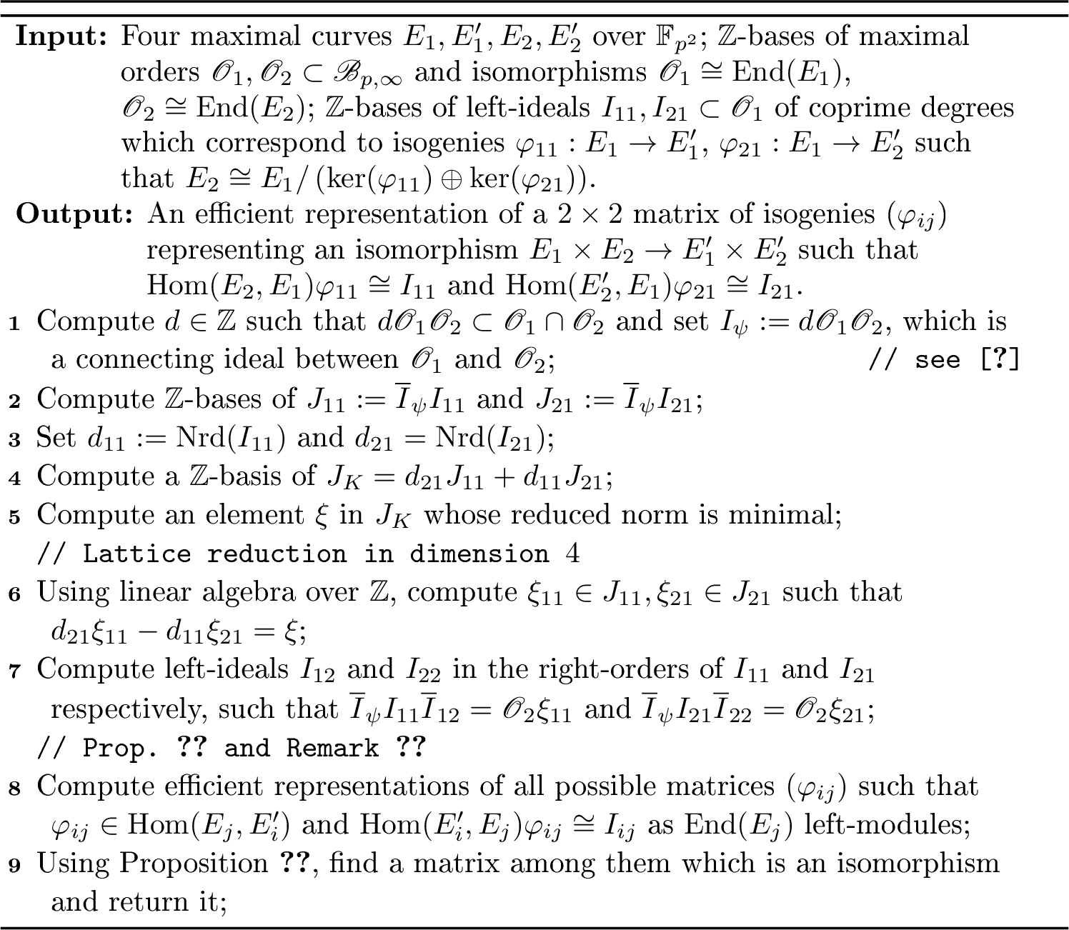
Theorem 25 is actually effective, provided that we know the endomorphism rings of the curves. Algorithm [algo:isomorphism95completion] computes such an isomorphism.
Proposition 26. Assuming GRH, Algorithm [algo:isomorphism95completion] is correct and it runs in time polynomial in \(\log(p)\) and in the size of the input.
Proof. First we prove that Algorithm [algo:isomorphism95completion] is correct. In fact, Algorithm [algo:isomorphism95completion] follows the proof of Theorem 25. An isogeny associated to the ideal \(I_\psi\) plays the role of \(\psi\) in the proof of Theorem 25. The ideals \(I_{11}\), \(I_{21}\) correspond to the isogenies \(\varphi_{11}, \varphi_{21}\) in Theorem 25, and the ideals \(J_{11}\) and \(J_{21}\) play the same role as in the proof of Theorem 25. We now prove that the endomorphism \(\xi\) computed in Step 2 satisfies the requirements of \(\sigma\) in the proof of Theorem 25, namely that \(\mathop{\mathrm{Nrd}}(\xi) = d_{11}d_{21}\mathop{\mathrm{Nrd}}(I_{\psi})\). By the same argument as in the proof of Theorem 25, \(J_K\) is a principal left-ideal (because \(E_1/K \simeq E_2\)) of reduced norm \(d_{11}d_{21}\mathop{\mathrm{Nrd}}(I_{\psi})\), so it contains an element with this reduced norm; this proves that \(\mathop{\mathrm{Nrd}}(\xi)= d_{11}d_{21}\mathop{\mathrm{Nrd}}(I_{\psi})\). Theorem 25 also asserts that at least one of the matrices computed at Step [step:automorphisms] is an isomorphism.
Let us now prove that the complexity is polynomial in the input size. Most steps reduce to \(\mathbb{Z}\)-linear algebra; this boils down to computing Hermite Normal Forms, which is done in time polynomial in the input size. Step 2 involves computing the shortest vector in a lattice of dimension \(4\), with the positive definite quadratic form \((x_1, x_2, x_3, x_4)\mapsto x_1^2 + x_2^2 + p(x_3^2 + x_4^2)\). This is done in time polynomial in the input size and in \(\log(p)\) [30]. The combinatorial factor in Step [step:automorphisms] does not increase the complexity since the number of possible isogenies \(E\to E'\) that are represented by the same left-ideal in \(\mathop{\mathrm{End}}(E)\) equals the order of \(\mathop{\mathrm{Aut}}(E)\). For most elliptic curves, \(\mathop{\mathrm{Aut}}(E) = \{1, -1\}\), and in any case \(\lvert\mathop{\mathrm{Aut}}(E)\rvert\leq 24\) [25]. Assuming GRH, converting the ideal representation to an efficient representation can be done in polynomial-time, see e.g. [24]. ◻
5.2.1 Experiments↩︎
We present the first part of our experimental results. We would like to emphasize that the goal of our proof-of-concept implementation is to illustrate the practicality of the algorithms and to provide experimental evidence of their correctness. Our
implementation is not optimized, and we do not claim that it is competitive in terms of speed and general efficiency. The presented results, as well as those described in Paragraph 5.3.1, are obtained runing our code under
Magma version V2.28-3, using a 13th Gen Intel Core i7-1365U CPU.
Let us describe the file ExperimentResults_part1.mgm available at [11]. We illustrate Algorithm [algo:isomorphism95completion], i.e., we compute an isomorphism \(E_0 \times E \to E_1' \times E_2'\), given isogenies \(\varphi_{11}:E_0 \to E_1'\) and \(\varphi_{21}:E_0 \to E_2'\) of coprime degree. Those isogenies are given by left \(\mathcal{O}_{0}\)-ideals, denoted \(I_{11}\) and \(I_{21}\) respectively.
First we let the user choose the following parameters: a lower bound for the prime \(p\), and the norm of the two ideals \(I_{11}\) and \(I_{21}\). Then we randomly compute such ideals, that determine (the isomorphism class of) \(E\) according to Theorem 25. We then recover the corresponding order \(\mathcal{O}_{}\simeq \mathop{\mathrm{End}}(E)\) as the right order of the left \(\mathcal{O}_{0}\)-ideal \(I_K:=d_{11}I_{21} + d_{21}I_{11}\), by application of Lemma 24. We conclude by computing the ideals \(I_{12}\) and \(I_{22}\), with a call to Algorithm [algo:isomorphism95completion]. We can finally check that the ideals \(I_{ij}\) represent an isomorphism, thanks to the following lemma.
Lemma 27. Let \(E_1,E_2,E_1',E_2'\) be elliptic curves defined over \(\overline{\mathbb{F}_p}\). For \(i,j\in\{1,2\}\), let \(\varphi_{ij}\in\mathop{\mathrm{Hom}}(E_j, E_i')\) be a morphism of degree \(d_{ij}\in\mathbb{Z}_{\geq 0}\). Denote \(\Phi:E_1 \times E_2 \to E_1' \times E_2'\) the \(2\)-dimensional morphism given by the matrix \((\varphi_{ij})_{ij}\). Let \(\psi:E_2 \to E_1\) be a nonzero morphism. Then \[\deg \begin{pmatrix} \varphi_{11} \circ \psi & \varphi_{12} \\ \varphi_{21} \circ \psi & \varphi_{22} \\ \end{pmatrix} = \deg(\psi) \deg(\Phi).\]
Proof. This is a direct consequence of Proposition 18. ◻
Example 28. We report on experimental results obtained by running the file ExperimentResults_part1.mgm with seed \(12345\). In this example, \(p=503\) and \(\ell_{11}=3\), \(m_{11}=6\) and \(\ell_{21}=5\), \(m_{21}=4\). We denote by \(1, i, j, k\) the usual generators of \(\mathcal{B}_{p,\infty}\). The input ideals are \(I_{11}= \langle 729, \, 729\, i, 321/2 + 553\,\, i + k/2, \, 553 + 1137 \, i/2 + j/2 \rangle\) of norm \(\ell_{11}^{m_{11}}\), and \(I_{21} = \langle 625, \, 625 \, i, \, 681/2 + 553\, i + k/2, \, 553 + 569\, i/2 + j/2 \rangle\) of norm \(\ell_{21}^{m_{21}}\). Then using Lemma 27, we check that the ideals \(I_{11}, I_{21}\), and \(I_{12} ,I_{22}\) returned by IsomorphismCompletion, represent an isomorphism.
With the same parameters \(p, \ell_{11}, m_{11}, \ell_{21}, m_{21}\), and averaging 100 unseeded runs of ExperimentResults_part1.mgm, we obtain a mean execution time of \(0.157\) seconds. The memory usage remains constant at \(32.09\)MB.
5.3 Computing isomorphisms \(E_0^2 \to E_1' \times E_0\)↩︎
In this section, we focus on a special \(2\)-dimensional instance of Problem 1: we assume that the endomorphism rings of all curves are known, and that we also know subrings of \(\mathop{\mathrm{End}}(E_1)\) and \(\mathop{\mathrm{End}}(E_1')\) which are isomorphic to a low-discriminant imaginary quadratic order. In this case, we provide a fast algorithm to compute the corresponding isomorphism, described in Algorithm [algo:isom1]. In order to simplify the exposition, we assume that \(E_1 = E_2 = E_2'\). In fact, this assumption does not lose any generality, see Remark 38. Also, for the sake of simplicity, we assume throughout this section that the curve for which we know a subring of endomorphisms isomorphic to a low-discriminant imaginary quadratic order is the curve \(E_0\) defined over \(\mathbb{F}_{p^2}\) (with \(p\equiv 3\bmod 4\)) by the equation \(y^2 = x^3+x\). Its endomorphism ring contains a subring isomorphic to \(\mathbb{Z}[i]\). However, all the results presented in this section can be generalized without any major difficulty to other curves. In particular, when \(p\equiv 1\bmod 4\), a curve with a low-discriminant can also be explicitly computed, see [20]. In summary, our objective in this section is to provide a fast algorithm for the following problem:
Problem 29 (Low-discriminant Deligne-Ogus-Shioda problem). Given a maximal supersingular elliptic curve \(E_1'\) defined over \(\mathbb{F}_{p^2}\) and its endomorphism ring, compute an \(\mathbb{F}_{p^2}\)-isomorphism \(E_0\times E_0\to E_1'\times E_0\).
The following statement gives sufficient conditions to use Theorem 25.
Proposition 30. Let \(E\), \(E_1'\) be elliptic curves defined over \(\overline{ \mathbb{F}_p}\) and let \(\varphi:E\to E_1'\) be a separable isogeny. Let \(\alpha, \nu\in \mathop{\mathrm{End}}(E)\) be endomorphisms of coprime degrees such that \(\deg(\alpha) = \deg(\varphi)\) and \(\alpha\nu\in \mathop{\mathrm{Hom}}(E_1', E)\varphi\). Then \(\ker(\nu)\oplus\ker(\varphi)\) is the kernel of the endomorphism \(\alpha\nu : E \to E\).
Proof. Since \(\alpha\nu\in \mathop{\mathrm{Hom}}(E_1', E)\varphi\), we have \(\ker(\varphi)\subset\ker(\alpha\nu)\). Consequently, \(\ker(\varphi)+\ker(\nu)\subset \ker(\alpha\nu)\). The co-primality of \(\deg(\nu)\) and \(\deg(\varphi)\) implies that the intersection of the kernels is trivial. Since \(\alpha\) and \(\nu\) are separable, so is \(\alpha\nu\) and hence \(\lvert\ker(\alpha\nu)\rvert = \deg(\alpha)\deg(\nu) = \deg(\varphi)\deg(\nu) = \lvert\ker(\varphi)\oplus\ker(\nu)\rvert\), which shows that the inclusion is in fact an equality. ◻
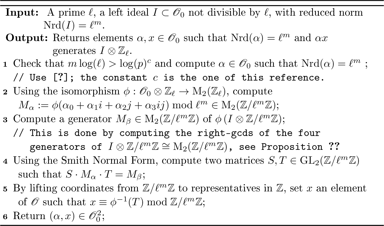
Proposition 30 tells us that if are able to compute \(\varphi, \alpha\) and \(\nu\), then Algorithm [algo:isomorphism95completion] can compute an isomorphism \(E \times E \to E_1' \times E\). Our strategy will be to first fix \(\varphi\), then to compute \(\alpha\) and \(\nu\) that satisfy the conditions of Proposition 30. As explained above, we specialize to the case \(E=E_0\), and \(p \equiv 3 \bmod 4\). The low-discriminant quadratic order will help us find the endomorphism \(\alpha \in \mathop{\mathrm{End}}(E_0)\) of prescribed degree \(\deg(\alpha)=\deg(\varphi)\) by solving low-discriminant norm equations with Cornacchia’s algorithm. Algorithm [algo:localgenerator] provides a fast method for computing such \(\alpha, \nu\) upon input of the ideal \(I\) corresponding to the isogeny \(\varphi\).
We start with technical lemmas which state that computing \(\alpha, \nu\) is related to computing a generator of a localization of the ideal \(I\) associated to \(\varphi\) at a prime \(\ell\).
Lemma 31. Let \(\mathcal{O}\subset \mathcal{B}_{p,\infty}\) be a maximal order, \(I\subset \mathcal{O}\) be a left ideal, \(\alpha \in \mathcal{O}\) such that \(\mathop{\mathrm{Nrd}}(\alpha)=\mathop{\mathrm{Nrd}}(I)\), and \(\ell\ne p\) be a prime number. Then the following statements are equivalent:
There exists \(x\in \mathcal{O}\), such that \(\alpha x\in I\) and \(\mathop{\mathrm{Nrd}}(x)\) is not divisible by \(\ell\);
There exists an invertible \(y\in \mathcal{O}\otimes \mathbb{Z}_{\ell}\) such that \(\alpha y\in I\otimes\mathbb{Z}_{\ell}\).
Proof. First, we notice that all elements \(x\in \mathcal{O}\) with reduced norm not divisible by \(\ell\) are invertible in \(\mathcal{O}\otimes \mathbb{Z}_\ell\); Indeed, \(x\cdot (\overline{x}/\mathop{\mathrm{Nrd}}(x)) = 1\), hence the inverse of \(x\) in \(\mathcal{O}\otimes \mathbb{Z}_\ell\) is \(\overline{x}/\mathop{\mathrm{Nrd}}(x)\). This proves the implication (a)\(\Rightarrow\)(b).
We now prove (b)\(\Rightarrow\)(a). Let \(y\) be as in (b). Let \(b_1,\ldots, b_4\) be generators of \(I\) seen as a free rank-\(4\) \(\mathbb{Z}\)-module. Then \(\alpha y=z_1\cdot b_1 + \cdots + z_4\cdot b_4\), with \(z_1, \ldots, z_4\in \mathbb{Z}_\ell\). Next, pick integers \(z_1',\ldots, z_4'\in \mathbb{Z}\) such that \(z_i'\equiv z_i\bmod \ell^e\), where \(e\) is the \(\ell\)-valuation of \(\mathop{\mathrm{Nrd}}(\alpha)\). Then set \(y'=\alpha^{-1}(z_1'\cdot b_1+\cdots + z_4'\cdot b_4)\in \mathcal{B}_{p,\infty}\). We prove now that \(x:=\mathop{\mathrm{Nrd}}(\alpha)y'/\ell^e\) satisfies the desired properties. First, we show that \(x = \ell^{-e}\overline{\alpha} (z_1'\cdot b_1+\cdots + z_4'\cdot b_4)\) belongs to \(\mathcal{O}\). Notice that \(x\) clearly belongs to localized orders \(\mathcal{O} \otimes \mathbb{Z}_{\ell'}\) for primes \(\ell'\neq \ell\), so we only have to prove that \(x\in\mathcal{O}\otimes \mathbb{Z}_\ell\). To do so, we use the fact that \(z_i\equiv z_i'\bmod \ell^e\), hence there exists \(z_1'',\ldots, z_4''\in\mathbb{Z}_\ell\) such that \(z_i = z_i'+\ell^e z_i''\), which gives \[\begin{array}{rcl}x &=& \ell^{-e}\overline{\alpha} (z_1\cdot b_1+\cdots + z_4\cdot b_4) - \overline{\alpha} (z_1''\cdot b_1 +\cdots+z_4''\cdot b_4)\\ &=& y \mathop{\mathrm{Nrd}}(\alpha)/\ell^e - \overline{\alpha} (z_1''\cdot b_1 +\cdots+z_4''\cdot b_4), \end{array}\] which shows that \(x\in\mathcal{O}\otimes\mathbb{Z}_\ell\). Then we notice that \(\mathop{\mathrm{Nrd}}(x)=(\mathop{\mathrm{Nrd}}(\alpha)/\ell^e)^2\mathop{\mathrm{Nrd}}(y')\) is not divisible by \(\ell\) since \(\mathop{\mathrm{Nrd}}(y')\equiv\mathop{\mathrm{Nrd}}(y)\not\equiv 0\bmod \ell\). Finally, since \(\mathop{\mathrm{Nrd}}(\alpha)=\mathop{\mathrm{Nrd}}(I)\in I\), we notice that \(\alpha x=\mathop{\mathrm{Nrd}}(\alpha)\ell^{-e}(z_1'\cdot b_1+\cdots + z_4'\cdot b_4)\) belongs to \(I\) ◻
Definition-Proposition 32. Let \(M\in \mathop{\mathrm{M}}_2(\mathbb{Z}_{\ell})\) be a matrix. We say that the \(\ell\)-type of \(M\) is the pair of valuations (in \(\mathbb{Z}_{\geq 0}^2\)) of the invariant factors of \(M\), sorted in non-decreasing order. More explicitly, using the Smith Normal Form, this means that \(M\) has \(\ell\)-type \((d_1,d_2)\) if \(d_1\leq d_2\) and if there exist invertible matrices \(S, T\in \mathop{\mathrm{GL}}_2(\mathbb{Z}_{\ell})\) such that \[S\cdot M\cdot T = \begin{pmatrix}\ell^{d_1}&0\\0&\ell^{d_2}\end{pmatrix}.\]
Since \(\mathop{\mathrm{M}}_2(\mathbb{Z}_{\ell})\) is left-principal, we define the \(\ell\)-type of a left-ideal \(I\subset \mathop{\mathrm{M}}_2(\mathbb{Z}_{\ell})\) as the \(\ell\)-type of a generator.
Let \(I\subset \mathcal{O}\) be a left-ideal of a maximal order in \(\mathcal{B}_{p,\infty}\), and \(\ell\ne p\) be a prime number. By [29], \(\mathcal{O}\otimes \mathbb{Z}_{\ell}\) is isomorphic to \(\mathop{\mathrm{M}}_2(\mathbb{Z}_{\ell})\), so we define the \(\ell\)-type of \(I\) as the \(\ell\)-type of \(I\otimes \mathbb{Z}_{\ell}\) regarded as an ideal in \(\mathop{\mathrm{M}}_2(\mathbb{Z}_{\ell})\); this definition does not depend on the choice of the isomorphism \(\mathcal{O}\otimes \mathbb{Z}_{\ell}\cong \mathop{\mathrm{M}}_2(\mathbb{Z}_{\ell})\). If \(\alpha\in \mathcal{O}\) is an element in a maximal order, its \(\ell\)-type is defined as the \(\ell\)-type of the left-ideal \(\mathcal{O}\alpha\).
Proof. The only thing that we need to prove is that the definition of the \(\ell\)-type of a left ideal \(I\subset\mathcal{O}\otimes\mathbb{Z}_\ell\cong\mathop{\mathrm{M}}_2(\mathbb{Z}_\ell)\) does not depend on the choice of the isomorphism. In fact, this is a consequence of the fact that automorphisms of \(\mathop{\mathrm{M}}_2(\mathbb{Z}_{\ell})\) preserve the \(\ell\)-type of matrices in \(\mathop{\mathrm{M}}_2(\mathbb{Z}_\ell)\), which can be seen on the Smith Normal Form since automorphisms act as conjugations by invertible matrices. ◻
Lemma 33. With the same notation as in Lemma 31, the \(\ell\)-types of \(I\) and \(\alpha\) are the same if and only if there exists an invertible \(y\in \mathcal{O}\otimes \mathbb{Z}_{\ell}\) such that \(\alpha y\in I\otimes\mathbb{Z}_{\ell}\).
Proof. In this proof, we fix an isomorphism \(\mathcal{O}\otimes \mathbb{Z}_\ell\cong \mathop{\mathrm{M}}_2(\mathbb{Z}_\ell)\) and we use it implicitly. Let \(\beta\in \mathop{\mathrm{M}}_2(\mathbb{Z}_\ell)\) be a generator of \(I\otimes \mathbb{Z}_\ell\).
To prove the “only if” part, we notice that if \(\alpha\) and \(\beta\) have the same invariant factors then there exist invertible matrices \(U, V\in\mathop{\mathrm{GL}}_2(\mathbb{Z}_\ell)\) such that \(U\cdot \beta= \alpha\cdot V\). This implies that \(\alpha\cdot V\) belongs to the left-ideal generated by \(\beta\). Writing \(y\in(\mathcal{O}\otimes\mathbb{Z}_\ell)^\times\) for the element corresponding to \(V\in\mathop{\mathrm{GL}}_2(\mathbb{Z}_\ell)\), we obtain \(\alpha y\in I\otimes \mathbb{Z}_\ell\).
We now prove the “if” part of the statement. Under the fixed isomorphism, the assumption \(\alpha y\in I\otimes\mathbb{Z}_\ell\) translates to the existence of \(U\in\mathop{\mathrm{M}}_2(\mathbb{Z}_\ell)\) such that \(\alpha y = U\beta\). By the multiplicativity of the determinant, we deduce that \(U\in\mathop{\mathrm{GL}}_2(\mathbb{Z}_\ell)\). Therefore \(\beta = U^{-1}\alpha y\) and hence \(\beta\) and \(\alpha\) have the same invariant factors. ◻
Lemma 34. With the same notation as in Lemma 31, if \(\alpha\in\mathcal{O}\) has \(\ell\)-type \((i, j)\), then there exists \(\alpha'\in\mathcal{O}\) with \(\ell\)-type \((0, j-i)\) such that \(\alpha = \ell^i\,\alpha'\). Similarly, if \(I\subset \mathcal{O}\) is a left-ideal which has \(\ell\)-type \((i,j)\), there exists a left-ideal \(I'\subset\mathcal{O}\) with \(\ell\)-type \((0, j-i)\) and \(I = \ell^i\cdot I'\).
Proof. Using Definition-Proposition 32, we just need to prove this property for matrices in \(\mathop{\mathrm{M}}_2(\mathbb{Z}_\ell)\). Let \(M\in\mathop{\mathrm{M}}_2(\mathbb{Z}_\ell)\) be a matrix with \(\ell\)-type \((i,j)\), i.e., there exists \(S,T\in\mathop{\mathrm{GL}}_2(\mathbb{Z}_\ell)\) such that \[S\cdot M\cdot T = \begin{pmatrix}\ell^{i}&0\\0&\ell^{j}\end{pmatrix}.\] Then set \(M' = S^{-1}\cdot \begin{pmatrix}1&0\\0&\ell^{j-i}\end{pmatrix}\cdot T^{-1}\), which has \(\ell\)-type \((0, j-i)\) and \(M=\ell^i M'\). ◻
We are now ready to prove the main algorithmic result of this section. It will rely on the fact that we can efficiently solve norm equations in \(\mathcal{O}_{0}\), if we assume that the norm to reach is big enough.
Theorem 35.
Assuming GRH, there exists a constant \(c>0\) such that on input an ideal \(I\) with \(\log(\mathop{\mathrm{Nrd}}(I)) > \log(p)^{c}\), Algorithm [algo:localgenerator] is correct and terminates in expected polynomial time in \(\log(p)\) and \(\log(\mathop{\mathrm{Nrd}}(I))\).
Proof. Let \(c\) be the constant given by [9], so that the corresponding algorithm can be run on input \(\mathop{\mathrm{Nrd}}(I)\). In [9], the algorithm is proved to be correct and polynomial time under GRH. Therefore \(\alpha\) can be correctly computed at Step 3. Hence the correctness of Algorithm [algo:localgenerator] is a direct consequence of Lemma 33 (to prove that the \(\ell\)-types of \(I\) and \(\alpha\) are the same) and of the proof of Lemma 34 which explains how to construct \(x\). The complexity is a consequence of the polynomial time computation of \(\alpha\), and of the fact that computing the Hermite Normal Forms (for computing the generator of \(I\otimes \mathbb{Z}/\ell^m\mathbb{Z}\)) and Smith Normal Forms of matrices in \(\mathop{\mathrm{M}}_2(\mathbb{Z}/\ell^m\mathbb{Z})\) can be done in quasi-linear complexity \(\widetilde{O}(m\log(\ell))\) [27]. ◻
Finally, we put all the pieces together and we give a complete algorithm (Algorithm [algo:isom1]) to compute an isomorphism \(E_0^2\to E_1'\times E_0\) upon input of \(E_1'\) and its endomorphism ring. In the following, \(c_0\) is the constant in Theorem 35.
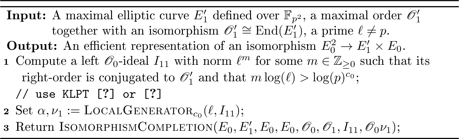
Theorem 36. Algorithm [algo:isom1] is correct and, under GRH, it requires an expected number of operations which is polynomial in \(\log(p)\).
Proof. The correctness is a consequence of Theorem 25 and Proposition 30, where Lemma 31 ensures that the output of LocalGenerator is valid data for the input of IsomorphismCompletion.The correctness of the subroutines are given in Theorem 35 and Proposition 26. The complexity follows from the complexities of the subroutines (Theorem 35 and Proposition 26), together with the fact that the output size of Wesolowski’s algorithm [9] is polynomial in \(\log(p)\). ◻
The following corollary shows that by running twice Algorithm [algo:isom1], we can compute isomorphisms \(E_1\times E_0\to E_2\times E_0\).
Corollary 37. Let \(E_1,E_2\) be maximal elliptic curves defined over \(\mathbb{F}_{p^2}\), with known endomorphism rings \(\mathcal{O}_{1}\cong \mathop{\mathrm{End}}(E_1)\) and \(\mathcal{O}_{2}\cong \mathop{\mathrm{End}}(E_2)\). Assuming GRH we can compute an efficient representation of an \(\mathbb{F}_{p^2}\)-isomorphism from \(E_1 \times E_0\) to \(E_2 \times E_0\) with a Las Vegas probabilistic algorithm running in expected polynomial time.
Proof. Running twice Algorithm [algo:isom1] provides us with efficient representations of two isomorphisms \(\xi_1 : E_0^2 \to E_1\times E_0\) and \(\xi_2: E_0^2\to E_2\times E_0\). By transposing \(\xi_2\) as in Section 4.3, we get an isomorphism \(\xi_2': E_2\times E_0\to E_0^2\). Finally, computing a efficient representation of \(\xi_1\circ \xi_2'\) provides the desired isomorphism. ◻
Remark 38. In fact, all results in this section generalize if we replace \(E_0\) by an elliptic curve \(E\) for which we know a subring of \(\mathop{\mathrm{End}}(E)\) isomorphic to a low-discriminant imaginary quadratic order. Corollary 37 can actually be generalized as follows: given \(E_1, E_2, E_1', E_2'\) supersingular elliptic curves defined over \(\mathbb{F}_{p^2}\) with their endomorphism rings, and given low-discriminant endomorphisms in \(\mathop{\mathrm{End}}(E_1)\) and \(\mathop{\mathrm{End}}(E_1')\), we can efficiently compute an isomorphism \(E_1\times E_2\to E_1'\times E_2'\) by computing isomorphisms \(E_1\times E_2\to E_1^2\), \(E_1^2\to E_1\times E_1'\), \(E_1\times E_1'\to (E_1')^2\), and \((E_1')^2\to E_1'\times E_2'\). Each isomorphism can be computed by using the low-discriminant technique described in this section.
5.3.1 Experiments↩︎
Let us describe an implementation of instances of Algorithm [algo:isom1] we propose in the file ExperimentResults_part2.mgm available at [11]. As in Section 5.2.1, the user can choose the parameters \(p,\ell\) and \(m\). Then we build a random ideal \(I_{11}\) such that \(\mathop{\mathrm{Nrd}}(I_{11})=\ell ^ m\). We recover \(\alpha\) and \(\nu_1\) with the function \(\textsf{LocalGenerator}\), where we compute \(\alpha\) with to Cornacchia’s algorithm. Those computations allow us to set \(I_{21}:= \mathcal{O}_{0} \nu_1\). Finally, as described in Algorithm [algo:isom1], we recover the two last ideals \(I_{12}\) and \(I_{22}\) by a call to IsomorphismCompletion. The function RepresentIsomorphism ensures that the computed ideals represent an isomorphism.
Example 39. We report on experimental results obtained by running Magma on the file ExperimentResults_part2.mgm with seed \(12345\). In this example,
\(p=503\), \(\ell=3\), \(m=7\). We denote by \(1, i, j, k\) the usual generators of \(\mathcal{B}_{p,\infty}\). The input ideal \(I_{11}\) has norm \(\ell^m\) and is given by the basis: \(\langle 2187, 2187\, i, 2863/2 +
1551\, i + k/2, 1551 + 1511\, i/2 + j /2 \rangle\). Computations give \(\alpha=30 + 28\, i - j\), and \(\nu_1=136567 - 12039/2 \, i + 5127 \, j/2 - 2160 \, k\). We set \(I_{21}:=\mathcal{O}_{0}\nu_1\). We finally check that RepresentIsomorphism returns True on the output of IsomorphismCompletion.
With the same parameters \(p, \ell\) and \(m\), and averaging 100 unseeded runs of ExperimentResults_part2.mgm, we obtain a mean execution time of \(1.125\) seconds. The memory usage remains constant at \(32.09\)MB.
5.4 Computing an isomorphism in the general case↩︎
For simplicity, we focus on the case \(p\equiv 3 \bmod 4\) where we can use the curve \(E_0\) defined over \(\mathbb{F}_{p^2}\) by the equation \(y^2 = x^3 + x\) which admits a low-discriminant endomorphism. If \(p\equiv 1\bmod 4\), we can use instead the construction described in [20].
First we provide an algorithm to solve a special case of Theorem 10.
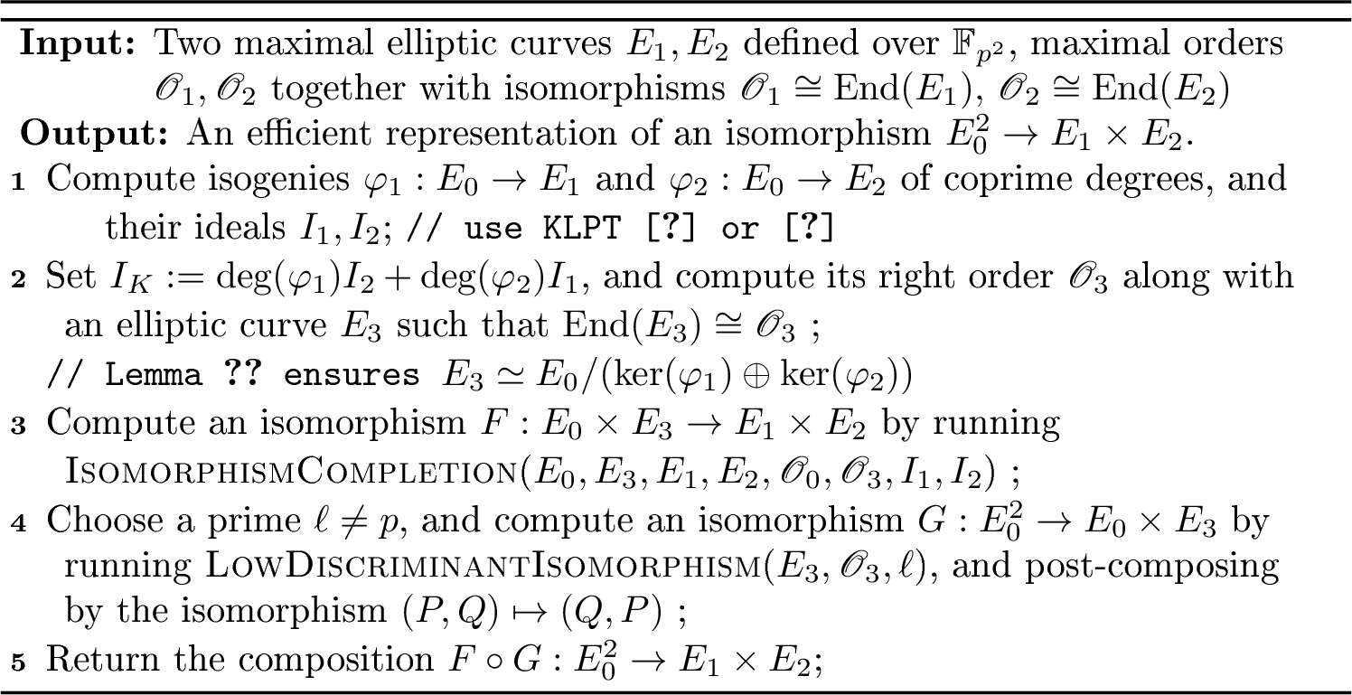

Theorem 40. Algorithm [algo:IsomorphismEO] is correct and assuming GRH it requires an expected number of operations which is polynomial in \(\log(p)\).
Proof. First we prove that the algorithm is correct. Since we know the endomorphism rings of \(E_0,E_1,E_2\) we can compute isogenies \(\varphi_i:E_0 \to E_i\) of coprime degrees by [9]. Applying Lemma 24 with \(\psi = Id_{E_0}\) leads to the construction of the ideal \(I_K\) representing an isogeny \(E_0 \to E_0/( \ker(\varphi_1) \oplus \ker(\varphi_2))\). The correctness is then a consequence of Proposition 26 and Theorem 36. The complexity follows from the same results, using the fact that [9] requires polynomial time assuming GRH, and that constructing \(I_K\) is standard \(\mathbb{Z}\)-linear algebra. ◻
We finally present a proof of Theorem 10.
Proof of Theorem 10. By two calls to Algorithm [algo:IsomorphismEO], we compute two isomorphisms \(\Phi: E_0^2 \to E_1 \times E_2\) and \(\Psi: E_0^2 \to E_1' \times E_2'\). Then by Corollary 20 we compute the tranposed isomorphism \(\widetilde{\Phi}:E_1 \times E_2 \to E_0^2\). Computing the composition \(\Psi \circ \widetilde{\Phi}\) leads to the desired isomorphism \(E_1 \times E_2 \to E_1' \times E_2'\). The complexity statement follows from Theorem 40. ◻