Keywords: neuro-symbolic AI, inductive logic programming, multi-instance partial label learning, weak supervision

1 Introduction↩︎

Weak supervision is an approach to machine learning for training models in settings where fully labelled data are limited. By reducing reliance on detailed labels, it enables models to learn from data that contain noise, ambiguity or missing labels [1]. However, the benefits of weak supervision come with challenges: models trained under weak supervision can lack reliability and diagnosability, especially without a structured logical framework to guide learning. This limitation is particularly concerning in high-stakes applications where model accountability matters [2], [3]. Zhou [1] categorizes weak supervision into three main types: incomplete supervision (only part of the data is labelled), inaccurate supervision (labels may contain errors) and inexact supervision (where labels are provided at a coarse-grained level). Within inexact supervision, multi-instance partial label learning (MI-PLL) is one such setting. MI-PLL combines multi-instance learning, where training samples consist of bags of instances, with partial label learning, where labels are ambiguous. In this setup, each training bag is associated with a candidate label set that includes at least one true label and potentially some false positives [4].

Wang et al. [5] proved sample-complexity bounds for classifier learnability in MI-PLL. Their work explored cases where transition functions are either known or unknown, extending the known-transition analysis to multiple classifiers across diverse domains. The analysis combines classical statistical learning theory (Vapnik–Chervonenkis (VC) and Natarajan dimensions, and Rademacher complexity) with a weighted-model-count semantic loss for symbolic-label structure, yielding both theoretical bounds and an empirical evaluation. Building directly on that line, Tsamoura et al. [6] extend the analysis to class-specific risk in MI-PLL, showing that the symbolic component \(\sigma\) can induce significant per-class learning imbalances even when the hidden gold-label distribution is uniform. Their class-specific risk bounds drop the \(M\)-unambiguity requirement of Wang et al.’s lemma 1 [5] and recover it in the \(M\)-unambiguous \(M = 2\) case (Tsamoura et al.’s proposition 3.4), constituting a strict generalization of the latter (Wang et al.’s [5] other learnability results, including the sample-complexity theorems 1 and 5 and proposition 1, and the Rademacher-style top-\(k\) surrogate theorem 2, are not subsumed). Together, these two works form the theoretical lineage on which the present framework builds: Wang et al. [5] supply the unambiguity conditions used to compare aggregation operators, and Tsamoura et al. [6] supply the class-specific risk framework that provides formal language for interpreting the operator-dependent failure modes observed empirically.

This paper proposes a semantics for a neuro-symbolic framework that uses inductive logic programming (ILP) [7] to structure MI-PLL through relational constraints. The objectives are threefold: first, to logically characterize the hypothesis space for learning the transition function, examining how weak supervision operates given coarse labels and neural classifier outputs; second, to develop a logical framework that formalizes classifier semantics, defining both the targets and the functionalities of classifiers within weakly supervised settings; and third, to define a standard for assessing model behaviour against those relational constraints.

By structuring weak supervision within ILP, the noisy and ambiguous outputs of that supervision are systematically organized into relational constraints. This semantics is proposed in general terms, independent of any specific neuro-symbolic system: at the architectural level it is a ‘Neuro \(\mid\) Symbolic’ system in Kautz’s [8] neuro-symbolic taxonomy, where the neural classifier maps non-symbolic image pixels to per-instance digit predictions and the CP/TP/OP machinery (the classifier predicate (CP), transition predicate (TP) and observed predicate (OP), formalized in §2b) then checks whether these predictions, the candidate transition rule and the bag-level observation are logically consistent. To test whether this semantics yields useful learning behaviour empirically, a differentiable pipeline in the style of the \(\alpha\)-ILP system is used as the experimental backend: the consistency check is made differentiable and gradients backpropagate to the classifier in joint training, which places the realization in Kautz’s ‘\(\text{Neuro}_{\text{Symbolic}}\)’ category (Kautz’s category for differentiable logic, into which differentiable ILP falls). The semantics is the proposal; the differentiable realization is the experimental methodology through which it is tested.

2 Logical foundations of weakly supervised induction↩︎

This section develops the logical foundations of the framework, introducing symbolic notation and the bag-level supervision setting (§2a), formalizing the MI-PLL problem with three auxiliary predicates CP, TP and OP (§2b) and describing ILP-based hypothesis induction in this setting (§2c).

2.1 Symbolic semantics of input data↩︎

MNIST handwritten-digit images serve as a running example throughout the paper [9], [10]. For each digit \(j \in \{0, \ldots, 9\}\),   denotes an MNIST image of that digit:

\[\fboxsep=1pt \fbox{\parbox[c][0.75em][c]{0.75em}{j}} \in \left\{ \raisebox{-0.15em}{\includegraphics[height=1.05em,trim=1 1 1 1,clip]{figures/MNIST_Digits/0.png}},\, \raisebox{-0.15em}{\includegraphics[height=1.05em,trim=1 1 1 1,clip]{figures/MNIST_Digits/1.png}},\, \raisebox{-0.15em}{\includegraphics[height=1.05em,trim=1 1 1 1,clip]{figures/MNIST_Digits/2.png}},\, \raisebox{-0.15em}{\includegraphics[height=1.05em,trim=1 1 1 1,clip]{figures/MNIST_Digits/3.png}},\, \raisebox{-0.15em}{\includegraphics[height=1.05em,trim=1 1 1 1,clip]{figures/MNIST_Digits/4.png}},\, \raisebox{-0.15em}{\includegraphics[height=1.05em,trim=1 1 1 1,clip]{figures/MNIST_Digits/5.png}},\, \raisebox{-0.15em}{\includegraphics[height=1.05em,trim=1 1 1 1,clip]{figures/MNIST_Digits/6.png}},\, \raisebox{-0.15em}{\includegraphics[height=1.05em,trim=1 1 1 1,clip]{figures/MNIST_Digits/7.png}},\, \raisebox{-0.15em}{\includegraphics[height=1.05em,trim=1 1 1 1,clip]{figures/MNIST_Digits/8.png}},\, \raisebox{-0.15em}{\includegraphics[height=1.05em,trim=1 1 1 1,clip]{figures/MNIST_Digits/9.png}}\right\}.\] Each   has ground-truth label \(j\), visible by inspection but treated as latent by the model. When   appears in two different bags, the occurrences are distinct exemplars of digit \(j\). Throughout the paper, \(j \in \{0, \ldots, 9\}\) ranges over digit values, while \(i \in \{1, \ldots, M\}\) indexes the position of an instance within a bag.

As the running example used in §2b, take the bag \(( \raisebox{-0.15em}{\includegraphics[height=1.05em,trim=1 1 1 1,clip]{figures/MNIST_Digits/2.png}}, \raisebox{-0.15em}{\includegraphics[height=1.05em,trim=1 1 1 1,clip]{figures/MNIST_Digits/3.png}})\). A bag is written as a tuple of the constituent images, so \(( \raisebox{-0.15em}{\includegraphics[height=1.05em,trim=1 1 1 1,clip]{figures/MNIST_Digits/2.png}}, \raisebox{-0.15em}{\includegraphics[height=1.05em,trim=1 1 1 1,clip]{figures/MNIST_Digits/3.png}})\) is the two-instance bag containing the images \(\raisebox{-0.15em}{\includegraphics[height=1.05em,trim=1 1 1 1,clip]{figures/MNIST_Digits/2.png}}\) and \(\raisebox{-0.15em}{\includegraphics[height=1.05em,trim=1 1 1 1,clip]{figures/MNIST_Digits/3.png}}\). Each image has an instance-level latent label: \(\text{label}( \raisebox{-0.15em}{\includegraphics[height=1.05em,trim=1 1 1 1,clip]{figures/MNIST_Digits/2.png}}) = 2\) and \(\text{label}( \raisebox{-0.15em}{\includegraphics[height=1.05em,trim=1 1 1 1,clip]{figures/MNIST_Digits/3.png}}) = 3\). Under the aggregation operator \(\sigma = +\) (sum), the bag is supervised by a single bag-level weak label \(s = \sigma(2, 3) = 5\), the only supervision the model receives. For compactness, the combined datum (the bag together with the observed weak label) is written as the sample form \(( \raisebox{-0.15em}{\includegraphics[height=1.05em,trim=1 1 1 1,clip]{figures/MNIST_Digits/2.png}}, \raisebox{-0.15em}{\includegraphics[height=1.05em,trim=1 1 1 1,clip]{figures/MNIST_Digits/3.png}}, 5)\): a tuple that lists the bag’s \(M\) instance images first, followed by the bag-level label \(s\); this is the same training datum that the predicate atom \(\text{OP}(( \raisebox{-0.15em}{\includegraphics[height=1.05em,trim=1 1 1 1,clip]{figures/MNIST_Digits/2.png}}, \raisebox{-0.15em}{\includegraphics[height=1.05em,trim=1 1 1 1,clip]{figures/MNIST_Digits/3.png}}), 5)\) records once predicates are introduced in §2b. In general, an MI-PLL training example has one latent instance-level label per image and one observed bag-level weak label per bag; the model must invert the aggregation across many bags to recover the instance labels (and, in some scenarios, the operator \(\sigma\)).

2.2 Problem structure and predicate formulation↩︎

Formally, an MI-PLL instance is a tuple \((X, Y, S, M, \sigma)\) where \(X \subseteq \mathbb{R}^n\) [1], [4] is the instance space, \(Y\) is a discrete label space, \(S\) is a bag-level label space, \(M \geq 1\) is a bag size and \(\sigma : Y^M \to S\) is an aggregation operator. A training sample is a pair \((\mathbf{x}, s) \in X^M \times S\), where \(\mathbf{x} = (x_1, \ldots, x_M)\) is a bag of \(M\) instances with latent gold-label vector \(\mathbf{y} = (y_1, \ldots, y_M) \in Y^M\) (one label \(y_i\) per instance \(x_i\)), and \(s = \sigma(\mathbf{y})\) is the bag-level weak label obtained by applying \(\sigma\) to \(\mathbf{y}\). Only \((\mathbf{x}, s)\) is observed by the learner; \(\mathbf{y}\) is hidden. The learner accesses a finite training set \(\mathcal{T}_{\textsf{P}} = \{(\mathbf{x}^{(b)}, s^{(b)})\}_{b=1}^{N}\) of \(N\) such samples drawn independently and identically distributed (i.i.d.) from a distribution \(\mathcal{D}_{\textsf{P}}\) over \(X^M \times S\). The operators used in this setup (\(\sigma \in \{+, \times, \oplus\}\)) are permutation-invariant in \(\mathbf{y}\); the Boolean operator \(C\) introduced in §3 (case 2 of scenario 2) is only partially permutation-invariant (lemma 2) and is included to illustrate how the framework extends to operators with distinguished argument positions.

The three relationships in this setup, per-instance prediction, aggregation and bag-level observation, are abstracted as three auxiliary logical predicates (atom is used throughout for a predicate applied to specific terms, e.g., \(\text{CP}(f, \raisebox{-0.15em}{\includegraphics[height=1.05em,trim=1 1 1 1,clip]{figures/MNIST_Digits/2.png}}, 2)\) is an atom of the CP predicate):

1. CP: for a classifier \(f : X \to Y\), the atom \(\text{CP}(f, x_i, y_i) \equiv f(x_i) = y_i\) records that \(f\) assigns label \(y_i \in Y\) to instance \(x_i \in X\). For an MNIST input, the CP atom takes the form \(\text{CP}(f, \fboxsep=1pt \fbox{\parbox[c][0.75em][c]{0.75em}{j}}, y)\) where \(y \in Y\) is the label assigned by \(f\); if \(f\) is correct, \(y\) equals the digit \(j\) shown by \(\fboxsep=1pt \fbox{\parbox[c][0.75em][c]{0.75em}{j}}\). For example, \(\text{CP}(f, \raisebox{-0.15em}{\includegraphics[height=1.05em,trim=1 1 1 1,clip]{figures/MNIST_Digits/2.png}}, 2)\) means \(f\) correctly predicts label \(2\) on the image \(\raisebox{-0.15em}{\includegraphics[height=1.05em,trim=1 1 1 1,clip]{figures/MNIST_Digits/2.png}}\); \(\text{CP}(f, \raisebox{-0.15em}{\includegraphics[height=1.05em,trim=1 1 1 1,clip]{figures/MNIST_Digits/2.png}}, 4)\) means \(f\) predicts label \(4\) on the same image, which is incorrect since the digit shown is \(2\). CP is the predicate inferred in scenario 2 of §3 (where \(\sigma\) is given and the per-instance assignment is learned).

2. TP: for the aggregation operator \(\sigma : Y^M \to S\) of the MI-PLL setup, the atom \(\text{TP}_\sigma(\mathbf{y}, s) \equiv \sigma(\mathbf{y}) = s\) records that \(\sigma\) maps the instance label vector \(\mathbf{y} \in Y^M\) to the bag label \(s \in S\). For example, \(\text{TP}_+((2, 3), 5)\) holds because \(2 + 3 = 5\), whereas \(\text{TP}_+((2, 3), 6)\) does not hold (\(2 + 3 \neq 6\)). TP is the predicate inferred in scenario 1 (where \(\sigma\) is unknown and chosen from a candidate set \(\Sigma\)).

3. OP: the atom \(\text{OP}(\mathbf{x}, s)\) records that the bag \(\mathbf{x} \in X^M\) is observed with weak label \(s \in S\); equivalently, \(\text{OP}(\mathbf{x}, s)\) holds for each training pair \((\mathbf{x}, s) \in \mathcal{T}_{\textsf{P}}\). For an MNIST bag, each \(x_i\) is a digit image; for example, \(\text{OP}(( \raisebox{-0.15em}{\includegraphics[height=1.05em,trim=1 1 1 1,clip]{figures/MNIST_Digits/2.png}}, \raisebox{-0.15em}{\includegraphics[height=1.05em,trim=1 1 1 1,clip]{figures/MNIST_Digits/3.png}}), 5)\) is the OP atom for the running training sample \(( \raisebox{-0.15em}{\includegraphics[height=1.05em,trim=1 1 1 1,clip]{figures/MNIST_Digits/2.png}}, \raisebox{-0.15em}{\includegraphics[height=1.05em,trim=1 1 1 1,clip]{figures/MNIST_Digits/3.png}}, 5)\), whereas \(\text{OP}(( \raisebox{-0.15em}{\includegraphics[height=1.05em,trim=1 1 1 1,clip]{figures/MNIST_Digits/2.png}}, \raisebox{-0.15em}{\includegraphics[height=1.05em,trim=1 1 1 1,clip]{figures/MNIST_Digits/3.png}}), 7)\) would not hold for that sample since the observed weak label is \(5\), not \(7\). OP is the only directly observable predicate and anchors the supervision.

Notation conventions (summary)

Two conventions apply throughout the paper: (i) a sample form \((x_1, \ldots, x_M, s)\) for enumerating training data, equivalent to the atom \(\text{OP}((x_1, \ldots, x_M), s)\) and (ii) an operator-subscript convention where the symbols \(\text{TP}\), \(\mathbb{I}\) and \(\mathbb{H}\) take a generic subscript (\(\text{TP}_\sigma, \mathbb{I}_\sigma\text{ and } \mathbb{H}_\sigma\)) when the operator is hypothesized or being searched over (scenario 1 of §3), and a specific subscript (\(\text{TP}_+, \text{TP}_\times, \text{TP}_\oplus, \text{TP}_C\), and likewise for \(\mathbb{I}\) and \(\mathbb{H}\)) when the operator is fixed and given (scenario 2). Full statements of both conventions are given in appendix B.

Continuing the running example from §2a, the training datum \(( \raisebox{-0.15em}{\includegraphics[height=1.05em,trim=1 1 1 1,clip]{figures/MNIST_Digits/2.png}}, \raisebox{-0.15em}{\includegraphics[height=1.05em,trim=1 1 1 1,clip]{figures/MNIST_Digits/3.png}}, 5)\) is recorded by the OP atom \(\text{OP}(( \raisebox{-0.15em}{\includegraphics[height=1.05em,trim=1 1 1 1,clip]{figures/MNIST_Digits/2.png}}, \raisebox{-0.15em}{\includegraphics[height=1.05em,trim=1 1 1 1,clip]{figures/MNIST_Digits/3.png}}), 5)\). Under \(\sigma = +\) with \(s = 5\), the TP atom \(\text{TP}_\sigma((y_1, y_2), 5)\) is satisfied by label pairs including \((5, 0)\), \((1, 4)\) and \((2, 3)\). Suppose the classifier \(f\) outputs the correct labels: \(f( \raisebox{-0.15em}{\includegraphics[height=1.05em,trim=1 1 1 1,clip]{figures/MNIST_Digits/2.png}}) = 2\) and \(f( \raisebox{-0.15em}{\includegraphics[height=1.05em,trim=1 1 1 1,clip]{figures/MNIST_Digits/3.png}}) = 3\), recorded by the CP atoms \(\text{CP}(f, \raisebox{-0.15em}{\includegraphics[height=1.05em,trim=1 1 1 1,clip]{figures/MNIST_Digits/2.png}}, 2)\) and \(\text{CP}(f, \raisebox{-0.15em}{\includegraphics[height=1.05em,trim=1 1 1 1,clip]{figures/MNIST_Digits/3.png}}, 3)\). Plugging the predicted labels into \(\sigma\) gives \(\sigma(2, 3) = 5 = s\), so \(\text{TP}_\sigma((2, 3), 5)\) holds and the three atoms \((\text{CP}, \text{TP}_\sigma\text{ and }\text{OP})\) are jointly satisfied. If instead \(f\) misclassifies (\(f( \raisebox{-0.15em}{\includegraphics[height=1.05em,trim=1 1 1 1,clip]{figures/MNIST_Digits/2.png}}) = 4\), \(f( \raisebox{-0.15em}{\includegraphics[height=1.05em,trim=1 1 1 1,clip]{figures/MNIST_Digits/3.png}}) = 2\)), the CP atoms become \(\text{CP}(f, \raisebox{-0.15em}{\includegraphics[height=1.05em,trim=1 1 1 1,clip]{figures/MNIST_Digits/2.png}}, 4)\) and \(\text{CP}(f, \raisebox{-0.15em}{\includegraphics[height=1.05em,trim=1 1 1 1,clip]{figures/MNIST_Digits/3.png}}, 2)\), and \(\sigma(4, 2) = 6 \neq 5\), so \(\text{TP}_\sigma((4, 2), 5)\) fails and the three atoms are inconsistent. This first example pairs every atom with both sample and predicate forms; subsequent examples enumerate training data in sample form and assemble predicate atoms inside constraint structures and consistency checks without restating the mapping. The pair of cases shown here illustrates the consistency check on a single bag; in practice, learning involves many bags and a hypothesis \(H = (f, \sigma)\) drawn from a search space, and the goal is to find an \(H\) under which the three atoms are jointly satisfied on as many bags as possible. Section 2c describes how ILP structures this search.

2.3 Inductive logic programming-based hypothesis induction↩︎

ILP is a relational learning framework that induces logic programs from data, using background knowledge to constrain the hypothesis space [7], [11]. Formally, given a background theory \(B\), a set of positive examples \(E^+\), and a set of negative examples \(E^-\), the goal is to find a hypothesis \(H\), a set of clauses, such that \(B \cup H \models e\) for all \(e \in E^+\), and \(B \cup H \not\models e\) for all \(e \in E^-\). The hypothesis \(H\) is drawn from a restricted language defined by a syntactic bias (e.g. mode declarations and maximum clause length), ensuring tractability and domain relevance.

MI-PLL is cast as an ILP problem with a structured hypothesis. A hypothesis is a pair \(H = (f, \sigma)\), where \(f : X \to Y\) is a classifier and \(\sigma\) is an aggregation operator drawn from the candidate set \(\Sigma\) (e.g. \(\Sigma = \{+, \times, \oplus, C\}\)). The background knowledge \(B\) encodes \(\Sigma\) together with each operator’s structural constraints (permutation invariance for \(+, \times, \oplus\); partial permutation invariance for \(C\); lemma 2). Each training bag \((\mathbf{x}, s) \in \mathcal{T}_{\textsf{P}}\) supplies the OP atom \(\text{OP}(\mathbf{x}, s)\) as supervision. Given a hypothesis \(H = (f, \sigma)\), each bag is classified as a positive example (\(\mathbf{x} \in E^+\)) if the CP atoms induced by \(f\) jointly satisfy \(\text{TP}_\sigma((f(x_1), \ldots, f(x_M)), s)\), and as a negative example (\(\mathbf{x} \in E^-\)) otherwise. The partition is therefore hypothesis-dependent; the formal definition is given in §3.

Learning in this setting is both partially observable and abductive. Since instance labels \(y_i\) are hidden, the learner must abduce latent CP and TP assignments such that these jointly entail the observed OP atoms; the resulting bag-by-bag conjunction is called an intermediate interpretation \(\mathbb{I}_\sigma\), parametrized by the operator under hypothesis. The ILP task is to search the hypothesis space \(\mathbb{H}\) of pairs \(H = (f, \sigma)\) for one whose intermediate interpretation \(\mathbb{I}_\sigma\) satisfies the supervision \(B \cup H \models \text{OP}(\mathbf{x}, s)\) on as many training bags as possible (§3 replaces this entailment reading with a hypothesis-dependent partition, since the OP atoms are observations rather than derivable facts).

To illustrate this process, consider four training examples in sample form: \(( \raisebox{-0.15em}{\includegraphics[height=1.05em,trim=1 1 1 1,clip]{figures/MNIST_Digits/2.png}}, \raisebox{-0.15em}{\includegraphics[height=1.05em,trim=1 1 1 1,clip]{figures/MNIST_Digits/3.png}}, 7)\), \(( \raisebox{-0.15em}{\includegraphics[height=1.05em,trim=1 1 1 1,clip]{figures/MNIST_Digits/1.png}}, \raisebox{-0.15em}{\includegraphics[height=1.05em,trim=1 1 1 1,clip]{figures/MNIST_Digits/4.png}}, 5)\), \(( \raisebox{-0.15em}{\includegraphics[height=1.05em,trim=1 1 1 1,clip]{figures/MNIST_Digits/5.png}}, \raisebox{-0.15em}{\includegraphics[height=1.05em,trim=1 1 1 1,clip]{figures/MNIST_Digits/2.png}}, 9)\) and \(( \raisebox{-0.15em}{\includegraphics[height=1.05em,trim=1 1 1 1,clip]{figures/MNIST_Digits/3.png}}, \raisebox{-0.15em}{\includegraphics[height=1.05em,trim=1 1 1 1,clip]{figures/MNIST_Digits/6.png}}, 8)\). Assuming the aggregation operator \(\sigma = +\), each pair of latent labels is hypothesized to sum to the corresponding weak label. Suppose \(f\) is a perfect classifier, so \(\text{CP}(f, \fboxsep=1pt \fbox{\parbox[c][0.75em][c]{0.75em}{j}}, j)\) holds for every digit \(j\). Bag 2 is then consistent under \(\sigma = +\) since \(\text{TP}_\sigma((1, 4), 5)\) holds. Bags 1, 3 and 4 fail: \(2 + 3 = 5 \neq 7\), \(5 + 2 = 7 \neq 9\) and \(3 + 6 = 9 \neq 8\). Thus, only Bag 2 is consistent with the hypothesized addition operator under these CP predictions.

More generally, the internal structure induced by this reasoning yields one positive clause and three violations. This symbolic structure is represented as a conjunction of classifier outputs and aggregation constraints under \(\sigma = +\), denoted by: \[\mathbb{I}_\sigma = \left( \begin{align} &\text{CP}(f, \raisebox{-0.15em}{\includegraphics[height=1.05em,trim=1 1 1 1,clip]{figures/MNIST_Digits/2.png}}, 2) \land \text{CP}(f, \raisebox{-0.15em}{\includegraphics[height=1.05em,trim=1 1 1 1,clip]{figures/MNIST_Digits/3.png}}, 3) \land \neg\,\text{TP}_\sigma((2, 3),\, 7) \\ \land\;& \text{CP}(f, \raisebox{-0.15em}{\includegraphics[height=1.05em,trim=1 1 1 1,clip]{figures/MNIST_Digits/1.png}}, 1) \land \text{CP}(f, \raisebox{-0.15em}{\includegraphics[height=1.05em,trim=1 1 1 1,clip]{figures/MNIST_Digits/4.png}}, 4) \land \text{TP}_\sigma((1, 4),\, 5) \\ \land\;& \text{CP}(f, \raisebox{-0.15em}{\includegraphics[height=1.05em,trim=1 1 1 1,clip]{figures/MNIST_Digits/5.png}}, 5) \land \text{CP}(f, \raisebox{-0.15em}{\includegraphics[height=1.05em,trim=1 1 1 1,clip]{figures/MNIST_Digits/2.png}}, 2) \land \neg\,\text{TP}_\sigma((5, 2),\, 9) \\ \land\;& \text{CP}(f, \raisebox{-0.15em}{\includegraphics[height=1.05em,trim=1 1 1 1,clip]{figures/MNIST_Digits/3.png}}, 3) \land \text{CP}(f, \raisebox{-0.15em}{\includegraphics[height=1.05em,trim=1 1 1 1,clip]{figures/MNIST_Digits/6.png}}, 6) \land \neg\,\text{TP}_\sigma((3, 6),\, 8) \end{align} \right).\]

This structure captures both satisfied and violated constraints under the hypothesized aggregation rule \(\sigma = +\). Such discrepancies help the ILP learner to assess the plausibility of \(\sigma\) as the governing rule. The resulting internal structure, denoted \(\mathbb{I}_\sigma\), serves as symbolic evidence that links classifier outputs (CP), instance-level label assignments and observed bag-level labels (OP) through an induced TP.

Constraint instances and conjunction

Each line contributing to \(\mathbb{I}_\sigma\) corresponds to a distinct constraint instance induced by a different bag. The conjunction notation denotes the collection of all such constraints across bags, rather than a single logical clause. Predicate atoms such as \(\mathrm{CP}(f,x,y)\) may therefore appear multiple times without redundancy, since each occurrence refers to a different data instance. Logical conjunction expresses the requirement that all bag-level constraints be considered simultaneously during hypothesis evaluation.

Inducing and evaluating \(\mathbb{I}_\sigma\) within the ILP framework generates symbolic hypotheses that link latent label assignments to the observed weak supervision. At the semantic level, ILP can be viewed as playing two complementary roles: a generative one, postulating plausible latent structures consistent with the weak supervision; a deductive one, filtering those structures by logical entailment of the observed OP atoms. The implementation realizes this view through differentiable soft marginalization over the TP and a bag-level cross-entropy loss against the observed weak labels, rather than through explicit symbolic abductive search; the predicate-level decomposition still describes what the joint training approximates. Section3 specializes the \((f, \sigma)\) decomposition into two scenarios: scenario 1 fixes \(f\) and infers \(\sigma\); scenario 2 fixes \(\sigma\) and infers \(f\).

3 Learning scenarios in multi-instance partial label learning↩︎

MI-PLL is formalized as an ILP task by encoding the hidden relationships between bag-level supervision and latent instance-level labels as logical hypotheses over the three predicates CP, TP and OP, forming a structured hypothesis space.

Two core learning scenarios are considered, each posing a different inductive task based on partial observability:

Scenario 1: inferring \(\text{TP}\) from \(\text{OP}\) and \(\text{CP.}\) This scenario captures the case where the weak label is known (OP), and instance-level predictions (CP) are assumed to be available. The goal is to discover a transition rule, captured by TP, that explains how instance labels collectively yield the bag-level label. \[H_{\text{TP}} \equiv \forall (\mathbf{x}, s) \in \mathcal{T}_{\textsf{P}}, \; \forall \mathbf{y} \in Y^M, \; \left( \text{OP}(\mathbf{x}, s) \land \bigwedge_{i=1}^{M} \text{CP}(f, x_i, y_i) \right) \Rightarrow \text{TP}_\sigma((y_1, \ldots, y_M), s), \label{eq:htp}\tag{1}\] where the label vector \(\mathbf{y}\) is universally quantified; since \(\text{CP}(f, x_i, \cdot)\) holds for exactly one value (\(y_i = f(x_i)\)), the formula is equivalent to requiring \(\text{TP}_\sigma((f(x_1), \ldots, f(x_M)), s)\) on every training bag, which is also the content of eqn (2 ) below; the two scenarios share this consistency condition and differ in which component (\(\sigma\) or \(f\)) is searched. Scenario 2: inferring \(\text{CP}\) from \(\text{OP}\) and \(\text{TP.}\) Here, the transition rule is treated as given, and the goal is to recover a classifier \(f\) whose per-instance predictions \(y_i := f(x_i)\) are jointly consistent with the bag-level label under the known TP. Writing \(\mathbf{f}(\mathbf{x}) := (f(x_1), \ldots, f(x_M))\), the hypothesis is given by: \[H_{\text{CP}} \equiv \forall (\mathbf{x}, s) \in \mathcal{T}_{\textsf{P}}, \; \text{OP}(\mathbf{x}, s) \;\Rightarrow\; \text{TP}_\sigma(\mathbf{f}(\mathbf{x}), s). \label{eq:hcp}\tag{2}\] Each hypothesis \(H = (f, \sigma)\) represents a structured explanation over latent components and is refined using sets of positive and negative examples (in both sets the latent labels are fixed by the classifier, \(y_i := f(x_i)\), which closes the formulas): \[E^+ = \Big\{ (\mathbf{x}, s) \in \mathcal{T}_{\textsf{P}} \;\Big|\; \text{OP}(\mathbf{x}, s) \land \bigwedge_{i=1}^{M} \text{CP}(f, x_i, y_i) \land \text{TP}_\sigma((y_1, \ldots, y_M), s) \Big\}\] \[\text{and }E^- = \Big\{ (\mathbf{x}, s) \in \mathcal{T}_{\textsf{P}} \;\Big|\; \text{OP}(\mathbf{x}, s) \land \bigwedge_{i=1}^{M} \text{CP}(f, x_i, y_i) \land \neg\,\text{TP}_\sigma((y_1, \ldots, y_M), s) \Big\}.\]

Hypotheses are evaluated against these examples, with the hypothesis language restricted by the background knowledge \(B\), optimizing the partition gap: \[\max_{H} \left( |E^+(H)| - |E^-(H)| \right).\]

This objective rewards hypotheses whose induced predictions cover as many observed OP atoms as possible while violating as few as possible; the entailment relation \(B \cup H \models e\) of classical ILP is replaced here by the hypothesis-dependent partition, since the OP atoms are observations rather than derivable facts.

Abductive partition

The sets \(E^+\) and \(E^-\) are hypothesis-dependent: each bag’s membership is determined by the CP predictions and TP rule contained in the current hypothesis \(H\). Unlike classical ILP, where \(E^+\) and \(E^-\) are static problem inputs, here, the partition shifts as the abduced latent assignments \(y_i\) and candidate operator \(\sigma\) evolve during search. The objective above is therefore a joint optimization over \(H\) and the induced partition that \(H\) defines.

Reduction under the (CP and TP) decomposition

Parametrizing \(H\) as a pair \((f, \sigma)\) makes the objective equivalent to bag-level classification accuracy on the weak labels: for every bag, \(\sigma(f(\mathbf{x}))=s\) places it in \(E^+\), otherwise in \(E^-\). Since \(|E^+| + |E^-|\) is the total number of supervised bags \(N\) (bags being pairwise distinct; appendix B), maximizing \(|E^+| - |E^-| = 2|E^+| - N\) is monotone in \(|E^+|\) and hence in bag accuracy. What this paper adds is therefore not the objective form but the structured hypothesis space: \(H\) decomposes into a neural classifier \(f\) (CP) and a symbolic operator \(\sigma\) (TP) drawn from a finite candidate set, with the search restricted by background knowledge \(B\), yielding a hypothesis whose internal structure is logically decomposed rather than monolithic.

3.1 Scenario 1: inferring the transition predicate↩︎

In this scenario, the goal is to infer the \(\text{TP}\) from the observed bag-level supervision \(\text{OP}\) and the instance-level classifier predictions \(\text{CP}\) as described in eqn (1 ). The true aggregation operator \(\sigma\) that maps instance labels to a bag label is not known in advance. Rather than assuming a fixed aggregation rule, a finite set of candidate operators \(\sigma \in \{+, \times, \oplus, C\}\) is considered, with the aim of identifying the operator that best explains the relationship between predicted instance labels and observed bag-level outputs. This is achieved by systematically evaluating each candidate \(\text{TP}_\sigma\) against the observed examples and selecting the most consistent TP.

Case 1 (\(\sigma = \times\)): consider four training examples in sample form: \(( \raisebox{-0.15em}{\includegraphics[height=1.05em,trim=1 1 1 1,clip]{figures/MNIST_Digits/2.png}}, \raisebox{-0.15em}{\includegraphics[height=1.05em,trim=1 1 1 1,clip]{figures/MNIST_Digits/3.png}}, 6)\), \(( \raisebox{-0.15em}{\includegraphics[height=1.05em,trim=1 1 1 1,clip]{figures/MNIST_Digits/4.png}}, \raisebox{-0.15em}{\includegraphics[height=1.05em,trim=1 1 1 1,clip]{figures/MNIST_Digits/3.png}}, 12)\), \(( \raisebox{-0.15em}{\includegraphics[height=1.05em,trim=1 1 1 1,clip]{figures/MNIST_Digits/5.png}}, \raisebox{-0.15em}{\includegraphics[height=1.05em,trim=1 1 1 1,clip]{figures/MNIST_Digits/2.png}}, 11)\) and \(( \raisebox{-0.15em}{\includegraphics[height=1.05em,trim=1 1 1 1,clip]{figures/MNIST_Digits/4.png}}, \raisebox{-0.15em}{\includegraphics[height=1.05em,trim=1 1 1 1,clip]{figures/MNIST_Digits/2.png}}, 7)\). Let the classifier \(f\) assign predictions: \(\text{CP}(f, \raisebox{-0.15em}{\includegraphics[height=1.05em,trim=1 1 1 1,clip]{figures/MNIST_Digits/2.png}}, 2)\), \(\text{CP}(f, \raisebox{-0.15em}{\includegraphics[height=1.05em,trim=1 1 1 1,clip]{figures/MNIST_Digits/3.png}}, 3)\), \(\text{CP}(f, \raisebox{-0.15em}{\includegraphics[height=1.05em,trim=1 1 1 1,clip]{figures/MNIST_Digits/4.png}}, 4)\) and \(\text{CP}(f, \raisebox{-0.15em}{\includegraphics[height=1.05em,trim=1 1 1 1,clip]{figures/MNIST_Digits/5.png}}, 5)\). Under the hypothesis that \(\sigma = \times\), the candidate predicate \(\text{TP}_\sigma\) is evaluated. Bags 1 and 2 are consistent: \(2 \times 3 = 6\), \(4 \times 3 = 12\). Bags 3 and 4, however, are inconsistent: \(5 \times 2 = 10 \neq 11\), \(4 \times 2 = 8 \neq 7\). Hence, \(\sigma = \times\) explains two of four examples.

\[\mathbb{I}_\sigma = \left( \begin{align} & \text{CP}(f, \raisebox{-0.15em}{\includegraphics[height=1.05em,trim=1 1 1 1,clip]{figures/MNIST_Digits/2.png}}, 2) \land \text{CP}(f, \raisebox{-0.15em}{\includegraphics[height=1.05em,trim=1 1 1 1,clip]{figures/MNIST_Digits/3.png}}, 3) \land \text{TP}_\sigma((2, 3), 6) \\ \land\;& \text{CP}(f, \raisebox{-0.15em}{\includegraphics[height=1.05em,trim=1 1 1 1,clip]{figures/MNIST_Digits/4.png}}, 4) \land \text{CP}(f, \raisebox{-0.15em}{\includegraphics[height=1.05em,trim=1 1 1 1,clip]{figures/MNIST_Digits/3.png}}, 3) \land \text{TP}_\sigma((4, 3), 12) \\ \land\;& \text{CP}(f, \raisebox{-0.15em}{\includegraphics[height=1.05em,trim=1 1 1 1,clip]{figures/MNIST_Digits/5.png}}, 5) \land \text{CP}(f, \raisebox{-0.15em}{\includegraphics[height=1.05em,trim=1 1 1 1,clip]{figures/MNIST_Digits/2.png}}, 2) \land \neg\,\text{TP}_\sigma((5, 2), 11) \\ \land\;& \text{CP}(f, \raisebox{-0.15em}{\includegraphics[height=1.05em,trim=1 1 1 1,clip]{figures/MNIST_Digits/4.png}}, 4) \land \text{CP}(f, \raisebox{-0.15em}{\includegraphics[height=1.05em,trim=1 1 1 1,clip]{figures/MNIST_Digits/2.png}}, 2) \land \neg\,\text{TP}_\sigma((4, 2), 7) \end{align} \right).\]

Case 2 (\(\sigma = +\)): consider four training examples in sample form: \(( \raisebox{-0.15em}{\includegraphics[height=1.05em,trim=1 1 1 1,clip]{figures/MNIST_Digits/4.png}}, \raisebox{-0.15em}{\includegraphics[height=1.05em,trim=1 1 1 1,clip]{figures/MNIST_Digits/7.png}}, 11)\), \(( \raisebox{-0.15em}{\includegraphics[height=1.05em,trim=1 1 1 1,clip]{figures/MNIST_Digits/3.png}}, \raisebox{-0.15em}{\includegraphics[height=1.05em,trim=1 1 1 1,clip]{figures/MNIST_Digits/6.png}}, 9)\), \(( \raisebox{-0.15em}{\includegraphics[height=1.05em,trim=1 1 1 1,clip]{figures/MNIST_Digits/2.png}}, \raisebox{-0.15em}{\includegraphics[height=1.05em,trim=1 1 1 1,clip]{figures/MNIST_Digits/9.png}}, 11)\) and \(( \raisebox{-0.15em}{\includegraphics[height=1.05em,trim=1 1 1 1,clip]{figures/MNIST_Digits/4.png}}, \raisebox{-0.15em}{\includegraphics[height=1.05em,trim=1 1 1 1,clip]{figures/MNIST_Digits/1.png}}, 6)\). The classifier’s predictions are given as: \(\text{CP}(f, \raisebox{-0.15em}{\includegraphics[height=1.05em,trim=1 1 1 1,clip]{figures/MNIST_Digits/4.png}}, 4)\), \(\text{CP}(f, \raisebox{-0.15em}{\includegraphics[height=1.05em,trim=1 1 1 1,clip]{figures/MNIST_Digits/7.png}}, 7)\), \(\text{CP}(f, \raisebox{-0.15em}{\includegraphics[height=1.05em,trim=1 1 1 1,clip]{figures/MNIST_Digits/3.png}}, 3)\), \(\text{CP}(f, \raisebox{-0.15em}{\includegraphics[height=1.05em,trim=1 1 1 1,clip]{figures/MNIST_Digits/6.png}}, 6)\), \(\text{CP}(f, \raisebox{-0.15em}{\includegraphics[height=1.05em,trim=1 1 1 1,clip]{figures/MNIST_Digits/2.png}}, 2)\), \(\text{CP}(f, \raisebox{-0.15em}{\includegraphics[height=1.05em,trim=1 1 1 1,clip]{figures/MNIST_Digits/9.png}}, 9)\) and \(\text{CP}(f, \raisebox{-0.15em}{\includegraphics[height=1.05em,trim=1 1 1 1,clip]{figures/MNIST_Digits/1.png}}, 1)\). Assuming \(\sigma = +\), bags 1–3 are satisfied: \(4 + 7 = 11\), \(3 + 6 = 9\), \(2 + 9 = 11\); bag 4 is violated: \(4 + 1 = 5 \neq 6\). The resulting structure is: \[\mathbb{I}_\sigma = \left( \begin{align} & \text{CP}(f, \raisebox{-0.15em}{\includegraphics[height=1.05em,trim=1 1 1 1,clip]{figures/MNIST_Digits/4.png}}, 4) \land \text{CP}(f, \raisebox{-0.15em}{\includegraphics[height=1.05em,trim=1 1 1 1,clip]{figures/MNIST_Digits/7.png}}, 7) \land \text{TP}_\sigma((4, 7), 11) \\ \land\;& \text{CP}(f, \raisebox{-0.15em}{\includegraphics[height=1.05em,trim=1 1 1 1,clip]{figures/MNIST_Digits/3.png}}, 3) \land \text{CP}(f, \raisebox{-0.15em}{\includegraphics[height=1.05em,trim=1 1 1 1,clip]{figures/MNIST_Digits/6.png}}, 6) \land \text{TP}_\sigma((3, 6), 9) \\ \land\;& \text{CP}(f, \raisebox{-0.15em}{\includegraphics[height=1.05em,trim=1 1 1 1,clip]{figures/MNIST_Digits/2.png}}, 2) \land \text{CP}(f, \raisebox{-0.15em}{\includegraphics[height=1.05em,trim=1 1 1 1,clip]{figures/MNIST_Digits/9.png}}, 9) \land \text{TP}_\sigma((2, 9), 11) \\ \land\;& \text{CP}(f, \raisebox{-0.15em}{\includegraphics[height=1.05em,trim=1 1 1 1,clip]{figures/MNIST_Digits/4.png}}, 4) \land \text{CP}(f, \raisebox{-0.15em}{\includegraphics[height=1.05em,trim=1 1 1 1,clip]{figures/MNIST_Digits/1.png}}, 1) \land \neg\,\text{TP}_\sigma((4, 1), 6) \end{align} \right).\]

In both illustrative cases, the underlying aggregation \(\sigma : Y^M \to S\) is a function, so \(\text{TP}\) is functional in \(\mathbf{y}\); however, \(\sigma\) may be non-injective, meaning that for a given bag label \(s\), the pre-image \(\sigma^{-1}(s) = \{\mathbf{y} \in Y^M : \sigma(\mathbf{y}) = s\}\) can contain multiple instance-label tuples. This non-injectivity (not the predicate form) is what permits multiple valid instance-to-bag mappings. For each candidate \(\sigma \in \{+, \times, \oplus, C\}\), a TP \(\text{TP}_\sigma\) is instantiated and evaluated using the observed supervision (\(\text{OP}\)) and classifier predictions (\(\text{CP}\)). This search process is formalized by selecting a candidate that maximizes consistency on the positive examples: choose \(\sigma \in \{+, \times, \oplus, C\}\) to maximize \[\bigl|\bigl\{(\mathbf{x}, s) \in \mathcal{T}_{\textsf{P}} \;:\; \text{TP}_\sigma((y_1, \ldots, y_M), s) \text{ holds with } y_i = f(x_i) \bigr\}\bigr|,\] where for each bag the latent labels are fixed by the CP atoms (\(y_i = f(x_i)\)). Negative examples \((\mathbf{x}, s) \in E^-\), when present, contribute through the dual condition \(\neg\,\text{TP}_\sigma((y_1, \ldots, y_M), s)\), so the joint ILP objective is the partition gap \(|E^+(\sigma)| - |E^-(\sigma)|\) of appendix B. The ILP engine then selects the most consistent and explanatory hypothesis \(\mathbb{H}_\sigma\), an operator-level hypothesis that explains bag-level labels via logical aggregation over instance-level predictions. This procedure systematically refines and validates symbolic hypotheses in weakly supervised settings.

Operator-by-operator learnability predictions

The MI-PLL learnability framework of Wang et al.[5] and the class-specific refinement by Tsamoura et al. [6] predict different difficulty regimes for each of the three operators through two structural conditions on \(\sigma\) from the former framework: \(M\)-unambiguity (distinct diagonal label vectors yield distinct bag labels) and the logically independent \(1\)-unambiguity (some position \(i\) such that flipping \(y_i\) always changes \(\sigma(\mathbf{y})\)). The three operators fall into three cells of this profile: \(\sigma = +\) is both \(1\)- and \(M\)-unambiguous (fastest sample-complexity rate of Wang et al.proposition 1 [5]); \(\sigma = \times\) is \(M\)-unambiguous but not \(1\)-unambiguous (the slower \(M\)-th-root rate of Wang et al.theorem 1 [5], and the formal condition associated with the multiplicative zero-attractor observed); \(\sigma = \oplus\) on \(M = 2\) is \(1\)-unambiguous but not \(M\)-unambiguous (no aggregate-risk bound applies; the configuration is consistent with the failure mode Wang et al.’s lemma 1 establishes existentially). Wang et al.’s [5] bounds are on sample complexity, not optimization dynamics; the empirical patterns are consistent with the predicted regimes rather than direct tests of those regimes. Full restatements, proofs and the detailed framework mapping are deferred to appendix C (Wang) and appendix D (Tsamoura’s class-specific extension via propositions 3.1 and 3.4).

3.2 Scenario 2: inferring the classifier predicate↩︎

In this scenario, the goal is to infer the classifier \(f : X \to Y\), recorded by the CP atoms \(\text{CP}(f, x_i, y_i)\) for each instance \(x_i\) in each training bag. The aggregation operator \(\sigma\) is assumed known and given by the fixed TP \(\text{TP}_\sigma\). Given observed OP atoms \(\text{OP}((x_1, x_2, \ldots), s)\) and a fixed \(\text{TP}_\sigma\), the task is to recover \(f\) so that the induced CP atoms are jointly consistent with the observed bag-level outcomes and the known transition rule.

Case 1 (\(\sigma = \oplus\), XOR aggregation): suppose the aggregation operator is known to be bitwise XOR, so the TP satisfies \(\text{TP}_\oplus((y_1, y_2), s) \equiv (y_1 \oplus y_2 = s)\). In this setting, the bag-level label is obtained by applying the XOR operation to the digit predictions of two MNIST images within each bag. Given the following training examples in sample form, \(( \raisebox{-0.15em}{\includegraphics[height=1.05em,trim=1 1 1 1,clip]{figures/MNIST_Digits/3.png}}, \raisebox{-0.15em}{\includegraphics[height=1.05em,trim=1 1 1 1,clip]{figures/MNIST_Digits/5.png}}, 6)\), \(( \raisebox{-0.15em}{\includegraphics[height=1.05em,trim=1 1 1 1,clip]{figures/MNIST_Digits/2.png}}, \raisebox{-0.15em}{\includegraphics[height=1.05em,trim=1 1 1 1,clip]{figures/MNIST_Digits/7.png}}, 5)\), \(( \raisebox{-0.15em}{\includegraphics[height=1.05em,trim=1 1 1 1,clip]{figures/MNIST_Digits/4.png}}, \raisebox{-0.15em}{\includegraphics[height=1.05em,trim=1 1 1 1,clip]{figures/MNIST_Digits/1.png}}, 5)\) and \(( \raisebox{-0.15em}{\includegraphics[height=1.05em,trim=1 1 1 1,clip]{figures/MNIST_Digits/6.png}}, \raisebox{-0.15em}{\includegraphics[height=1.05em,trim=1 1 1 1,clip]{figures/MNIST_Digits/7.png}}, 1)\), the digit label for each instance is to be inferred such that these relationships hold. This leads to the following internal constraint structure:

\[\mathbb{I}_\oplus = \left( \begin{align} &\text{CP}(f, \raisebox{-0.15em}{\includegraphics[height=1.05em,trim=1 1 1 1,clip]{figures/MNIST_Digits/3.png}}, y_1) \land \text{CP}(f, \raisebox{-0.15em}{\includegraphics[height=1.05em,trim=1 1 1 1,clip]{figures/MNIST_Digits/5.png}}, y_2) \land \text{TP}_\oplus((y_1, y_2), 6) \\ \land\;&\text{CP}(f, \raisebox{-0.15em}{\includegraphics[height=1.05em,trim=1 1 1 1,clip]{figures/MNIST_Digits/2.png}}, y_3) \land \text{CP}(f, \raisebox{-0.15em}{\includegraphics[height=1.05em,trim=1 1 1 1,clip]{figures/MNIST_Digits/7.png}}, y_4) \land \text{TP}_\oplus((y_3, y_4), 5) \\ \land\;&\text{CP}(f, \raisebox{-0.15em}{\includegraphics[height=1.05em,trim=1 1 1 1,clip]{figures/MNIST_Digits/4.png}}, y_5) \land \text{CP}(f, \raisebox{-0.15em}{\includegraphics[height=1.05em,trim=1 1 1 1,clip]{figures/MNIST_Digits/1.png}}, y_6) \land \text{TP}_\oplus((y_5, y_6), 5) \\ \land\;&\text{CP}(f, \raisebox{-0.15em}{\includegraphics[height=1.05em,trim=1 1 1 1,clip]{figures/MNIST_Digits/6.png}}, y_7) \land \text{CP}(f, \raisebox{-0.15em}{\includegraphics[height=1.05em,trim=1 1 1 1,clip]{figures/MNIST_Digits/7.png}}, y_4) \land \text{TP}_\oplus((y_7, y_4), 1) \end{align} \right).\]

This constraint structure is now examined under the XOR operation. The first bag label \(6\) is explained by the pair \(3 \oplus 5 = 6\), the second by \(2 \oplus 7 = 5\), the third by \(4 \oplus 1 = 5\) and the fourth by \(6 \oplus 7 = 1\). These assignments jointly satisfy all bag-level XOR constraints, resulting in the classifier predictions: \(\text{CP}(f, \raisebox{-0.15em}{\includegraphics[height=1.05em,trim=1 1 1 1,clip]{figures/MNIST_Digits/3.png}}, 3)\), \(\text{CP}(f, \raisebox{-0.15em}{\includegraphics[height=1.05em,trim=1 1 1 1,clip]{figures/MNIST_Digits/5.png}}, 5)\), \(\text{CP}(f, \raisebox{-0.15em}{\includegraphics[height=1.05em,trim=1 1 1 1,clip]{figures/MNIST_Digits/2.png}}, 2)\), \(\text{CP}(f, \raisebox{-0.15em}{\includegraphics[height=1.05em,trim=1 1 1 1,clip]{figures/MNIST_Digits/7.png}}, 7)\), \(\text{CP}(f, \raisebox{-0.15em}{\includegraphics[height=1.05em,trim=1 1 1 1,clip]{figures/MNIST_Digits/4.png}}, 4)\), \(\text{CP}(f, \raisebox{-0.15em}{\includegraphics[height=1.05em,trim=1 1 1 1,clip]{figures/MNIST_Digits/1.png}}, 1)\) and \(\text{CP}(f, \raisebox{-0.15em}{\includegraphics[height=1.05em,trim=1 1 1 1,clip]{figures/MNIST_Digits/6.png}}, 6)\). Hence, the consistent classifier hypothesis under XOR aggregation is given by \(\mathbb{H}_{\oplus} \equiv \forall (\mathbf{x}, s) \in \mathcal{T}_{\textsf{P}}, \; \text{OP}(\mathbf{x}, s) \Rightarrow \text{TP}_\oplus(\mathbf{f}(\mathbf{x}), s)\), the form of eqn (2 ) specialized to \(\sigma = \oplus\) (writing \(\mathbf{f}(\mathbf{x}) = (f(x_1), \ldots, f(x_M))\)), meaning that the per-instance predictions \(f(x_i)\) are jointly consistent with the observed bag label under XOR.

The classifier predictions listed above are the witness for this hypothesis: under them every bag’s XOR equals its observed label, so \(\text{TP}_\oplus(\mathbf{f}(\mathbf{x}), s)\) holds for all four bags.

Case 2 (\(\sigma = C\), Boolean formula aggregation): now consider a scenario where the TP is governed by a Boolean formula \(\sigma_C(y_1, y_2, y_3) := (y_1 \land y_2) \lor (y_1 \land y_3)\), so \(\text{TP}_C((y_1, y_2, y_3), s) \equiv \sigma_C(y_1, y_2, y_3) = s\), with instance-level values restricted to \(\{0, 1\}\). Note that \(\text{TP}_C\) is symmetric in \(y_2\) and \(y_3\) but distinguishes \(y_1\); it is therefore only partially permutation-invariant. This case is retained as a theoretical illustration of how hypothesis complexity grows when symbolic structure is non-uniform across instance positions. The experimental evaluation in §4 restricts attention to fully permutation-invariant operators (\(+, \times, \oplus\)); operators with distinguished argument positions (such as \(\text{TP}_C\), subtraction and division) require an order-aware TP formulation and are left for future work. Given the following training examples in sample form, \(( \raisebox{-0.15em}{\includegraphics[height=1.05em,trim=1 1 1 1,clip]{figures/MNIST_Digits/1.png}}, \raisebox{-0.15em}{\includegraphics[height=1.05em,trim=1 1 1 1,clip]{figures/MNIST_Digits/3.png}}, \raisebox{-0.15em}{\includegraphics[height=1.05em,trim=1 1 1 1,clip]{figures/MNIST_Digits/2.png}}, 1)\), \(( \raisebox{-0.15em}{\includegraphics[height=1.05em,trim=1 1 1 1,clip]{figures/MNIST_Digits/2.png}}, \raisebox{-0.15em}{\includegraphics[height=1.05em,trim=1 1 1 1,clip]{figures/MNIST_Digits/3.png}}, \raisebox{-0.15em}{\includegraphics[height=1.05em,trim=1 1 1 1,clip]{figures/MNIST_Digits/4.png}}, 0)\), \(( \raisebox{-0.15em}{\includegraphics[height=1.05em,trim=1 1 1 1,clip]{figures/MNIST_Digits/1.png}}, \raisebox{-0.15em}{\includegraphics[height=1.05em,trim=1 1 1 1,clip]{figures/MNIST_Digits/4.png}}, \raisebox{-0.15em}{\includegraphics[height=1.05em,trim=1 1 1 1,clip]{figures/MNIST_Digits/3.png}}, 1)\) and \(( \raisebox{-0.15em}{\includegraphics[height=1.05em,trim=1 1 1 1,clip]{figures/MNIST_Digits/2.png}}, \raisebox{-0.15em}{\includegraphics[height=1.05em,trim=1 1 1 1,clip]{figures/MNIST_Digits/1.png}}, \raisebox{-0.15em}{\includegraphics[height=1.05em,trim=1 1 1 1,clip]{figures/MNIST_Digits/4.png}}, 0)\), the aim is to infer binary predictions per instance that collectively satisfy the Boolean structure. This gives rise to the constraint formula: \[\mathbb{I}_{C} = \left( \begin{align} &\text{CP}(f, \raisebox{-0.15em}{\includegraphics[height=1.05em,trim=1 1 1 1,clip]{figures/MNIST_Digits/1.png}}, y_1) \land \text{CP}(f, \raisebox{-0.15em}{\includegraphics[height=1.05em,trim=1 1 1 1,clip]{figures/MNIST_Digits/3.png}}, y_2) \\ \land\; &\text{CP}(f, \raisebox{-0.15em}{\includegraphics[height=1.05em,trim=1 1 1 1,clip]{figures/MNIST_Digits/2.png}}, y_3) \land \text{CP}(f, \raisebox{-0.15em}{\includegraphics[height=1.05em,trim=1 1 1 1,clip]{figures/MNIST_Digits/4.png}}, y_4) \\ \land\; &\text{TP}_C((y_1, y_2, y_3), 1) \land \text{TP}_C((y_3, y_2, y_4), 0) \\ \land\; &\text{TP}_C((y_1, y_4, y_2), 1) \land \text{TP}_C((y_3, y_1, y_4), 0) \end{align} \right).\]

One solution to this constraint structure assigns \(\text{CP}(f, \raisebox{-0.15em}{\includegraphics[height=1.05em,trim=1 1 1 1,clip]{figures/MNIST_Digits/1.png}}, 1)\), \(\text{CP}(f, \raisebox{-0.15em}{\includegraphics[height=1.05em,trim=1 1 1 1,clip]{figures/MNIST_Digits/2.png}}, 0)\), \(\text{CP}(f, \raisebox{-0.15em}{\includegraphics[height=1.05em,trim=1 1 1 1,clip]{figures/MNIST_Digits/3.png}}, 1)\) and \(\text{CP}(f, \raisebox{-0.15em}{\includegraphics[height=1.05em,trim=1 1 1 1,clip]{figures/MNIST_Digits/4.png}}, 0)\). Under this assignment, the Boolean formula \((y_1 \land y_2) \lor (y_1 \land y_3)\) evaluates to \(1\), \(0\), \(1\) and \(0\) for the four bags, respectively: specifically, \((1 \land 1) \lor (1 \land 0) = 1\), \((0 \land 1) \lor (0 \land 0) = 0\), \((1 \land 0) \lor (1 \land 1) = 1\) and \((0 \land 1) \lor (0 \land 0) = 0\). These match all observed bag-level labels.

This yields the classifier hypothesis \(\mathbb{H}_C \equiv \forall (\mathbf{x}, s) \in \mathcal{T}_{\textsf{P}}, \; \text{OP}(\mathbf{x}, s) \Rightarrow \text{TP}_C(\mathbf{f}(\mathbf{x}), s)\), again the form of eqn (2 ) specialized to \(\sigma = C\).

These case analyses illustrate how the task of inferring \(\text{CP}\) is shaped by the structural complexity of the TP \(\text{TP}_\sigma\). While the hypothesis for addition requires relatively straightforward additive consistency, those for multiplication, XOR (\(\mathbb{H}_{\oplus}\)) and Boolean aggregation (\(\mathbb{H}_C\)) demand increasingly complex symbolic reasoning. As the complexity of the aggregation rule increases, the ILP engine must operate over tighter and more expressive hypothesis spaces to maintain logical consistency between instance-level assignments and observed bag-level outputs.

4 Experiments and evaluation↩︎

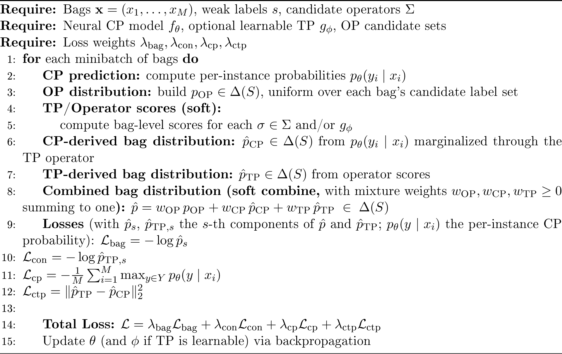
To operationalize the proposed OP–CP–TP semantics, the experiments use a differentiable pipeline in the style of \(\alpha\)-ILP, the differentiable ILP framework that integrates neural predicates with symbolic hypothesis scoring via differentiable logical reasoning [12]. The realization here follows that design rather than invoking the full clause-induction machinery: neural predicates instantiate the CP, differentiable marginalization through the candidate operators scores TP hypotheses, and the OP facts enter as soft constraints (algorithm 2).

In the experiments, this pipeline serves as an execution substrate for testing the proposed semantics rather than as the contribution. Neural perception is used to instantiate the CP from raw images, while symbolic reasoning is used to represent and select TPs from a predefined operator space. Weak supervision enters exclusively through OPs, which are treated as logical constraints rather than direct training targets. The pipeline enforces consistency among these components by favouring hypotheses whose induced CP and TP assignments jointly entail the observed OP facts.

The semantic claims do not rely on any architectural feature specific to this realization. Any neurosymbolic system capable of (i) explicitly representing CP, TP and OP as distinct predicates, (ii) reasoning over symbolic hypothesis spaces, and (iii) enforcing logical consistency under weak supervision could, in principle, instantiate the same semantics. The differentiable pipeline provides a concrete realization that allows these dependencies to be empirically evaluated.

The experimental design intentionally focuses on simple MI-PLL tasks in order to isolate semantic dependencies and make failure modes observable, rather than to maximize raw predictive performance.

4.1 Experimental setup↩︎

The framework is evaluated on MI-PLL datasets constructed from MNIST digit bags. Each bag contains exactly two digit images with hidden instance labels. The only supervision provided during training is a weak bag-level label, obtained by applying a symbolic aggregation operator to the latent instance labels. The experiments reported below cover the operator set, \[\sigma \in \{+, \times, \oplus\},\] chosen to span the Wang et al.[5] unambiguity profile discussed in appendix C.2: addition satisfies both \(1\)- and \(M\)-unambiguity, multiplication satisfies \(M\)- but not \(1\)-unambiguity and XOR satisfies \(1\)- but not \(M\)-unambiguity. The choice also probes the class-specific imbalance regime characterized by Tsamoura et al. [6]: multiplication on the digit range has an asymmetric pre-image distribution (the bag label \(s = 0\) absorbs 19 of the 100 ordered pairs) while addition and XOR have flatter pre-image profiles, so operator-by-operator differences in OP-noise tolerance and per-class collapse become legible against the Tsamoura et al.framework (appendix D). The evaluation restricts to fully permutation-invariant operators here; order-sensitive operators (subtraction and division) and the Boolean formula \(\mathrm{TP}_C\) used illustratively in §3b require an order-aware TP and are left for future work.

In the implementation, CP is realized as a convolutional neural network, TP is drawn from a discrete hypothesis space of symbolic operators and the pipeline mediates the CP–TP interaction by enforcing the CP/TP/OP consistency constraint of §2b and selecting consistent hypotheses. All reported results are averaged over multiple random seeds (20 runs for experiments 1 and 2, and 10 runs for the OP-noise study), reported as mean \(\pm\) standard deviation.

Training details

Each run uses \(N_\text{train} = 2000\) training bags and \(N_\text{val} = 500\) validation bags drawn from MNIST. Supervision for each training bag is a candidate set of size \(3\) containing the true weak label \(s_b\) and two distractor labels drawn from the feasible bag-label range of \(\sigma\); the OP distribution \(p_{\text{OP}}\) of algorithm 2 is uniform over this set. This realizes the candidate-set form of MI-PLL supervision (§1) with the aggregated label of §2b as the guaranteed true member. The weak label itself is left uncorrupted in experiments 1 and 2; only the OP-noise study replaces \(s_b\) at the stated corruption rates, and all validation metrics are computed against clean weak labels throughout. The CP convolutional network is trained with Adam at a learning rate of \(10^{-3}\) and batch size \(64\). The epoch budget is \(15\) for the scenario-2 driver (tables ¿tbl:tab:unified95ablation? and ¿tbl:tab:exp295cp?), \(10\) CP-warm followed by \(15\) TP-discovery epochs for the scenario-1 driver (table ¿tbl:tab:exp195tp?) and \(8\) CP-warm followed by \(15\) TP-discovery epochs for the OP-noise study (table ¿tbl:tab:op95noise?). In the scenario-1 drivers, the CP-warm phase trains the classifier under the true operator (the scenario-2 configuration); TP discovery then freezes the classifier and trains only the operator weights (§4c). The algorithm 2 four-term loss is applied with weights \((\lambda_{\text{bag}}, \lambda_{\text{con}}, \lambda_{\text{cp}}, \lambda_{\text{ctp}}) = (1.0,\;1.0,\;0.05,\;0.5)\) and the CP–TP distance realized as squared \(\ell_2\) between the CP-derived and TP-derived bag distributions. Auxiliary entropy and ILP-style regularizers are kept disabled (weight zero) to keep the loss exactly the four terms displayed in algorithm 2; adding these auxiliary terms with non-zero weights was found to destabilize scenario-2 training on the non-\(1\)-unambiguous operator \(\sigma = \times\).

Metrics

Let \(\mathcal{B}\) be the validation set of \(N_{\text{val}}\) bags, each of size \(M\). For bag \(b\), write \(s_b\) for the observed bag label, \(\hat{s}_b = \arg\max_t \hat{p}_t\) for the predicted bag label (the argmax of the combined bag distribution \(\hat{p}\) of algorithm 2), \(y_{b,i}\) for the (held-out) gold instance label at position \(i\) and \(\hat{y}_{b,i} = \arg\max_y p_\theta(y \mid x_{b,i})\) (the per-instance CP probability of algorithm 2) for the predicted instance label. The reported metrics are:

1. BagAcc \(= \tfrac{1}{N_{\text{val}}} \sum_b \mathbf{1}\{\hat{s}_b = s_b\}\): correctness at the weak-supervision level.

2. InstAcc \(= \tfrac{1}{N_{\text{val}}M} \sum_b \sum_{i=1}^{M} \mathbf{1}\{\hat{y}_{b,i} = y_{b,i}\}\): alignment with latent instance-level labels.

3. Constraint \(= \tfrac{1}{N_{\text{val}}} \sum_b \mathbf{1}\{\sigma(\hat{y}_{b,1}, \ldots, \hat{y}_{b,M}) = s_b\}\): fraction of bags whose hard predicted instance labels satisfy the induced TP rule.

4. Bag–Constraint \(= \mathrm{BagAcc}-\mathrm{Constraint}\): a positive gap signals bag-level success that is not structurally supported by the induced TP rule (e.g.an OP\(\leftrightarrow\)TP shortcut).

5. Bag–Inst \(= \mathrm{BagAcc}-\mathrm{InstAcc}\): a positive gap signals misalignment between bag predictions and instance semantics (e.g.correct sums from wrong digits).

Evaluation pathways

BagAcc and Constraint are computed on different pipelines. BagAcc evaluates the combined distribution \(\hat{p}\) of algorithm 2, which mixes the TP-marginalized CP prediction with the OP candidate distribution at mixture weight \(w_{\text{OP}}\) (initialized at \(0.3\) and learned jointly in the scenario-2 runs; fixed at \(0.3\) in the scenario-1 drivers; algorithm 2 states the general three-weight combination, of which the evaluated configuration is the two-component form with \(w_{\text{TP}} = 0\)); since the candidate set contains the true label, the OP component places probability \(1/3\) on \(s_b\) and assists \(\hat{s}_b\). Constraint applies \(\sigma\) to the hard per-instance CP predictions with no OP contribution. A positive Bag–Constraint gap can therefore reflect either an OP\(\leftrightarrow\)TP shortcut or the OP-mixture assistance in \(\hat{s}_b\); reading it together with InstAcc separates the two. In the ‘no TP’ and ‘OP only’ ablations the bag prediction is produced by a direct bag classifier over the CP outputs, without access to the candidate distribution, so those rows are not assisted by OP at evaluation.

For TP inference (experiment 1), the following per-operator quantities are further defined. Given the candidate operator set \(\Sigma\) and predicted instance labels \(\hat{y}_{b,i}\), let \(E^+(\sigma) = \{b \in \mathcal{B} : \sigma(\hat{y}_{b,1}, \ldots, \hat{y}_{b,M}) = s_b\}\) and \(E^-(\sigma) = \mathcal{B} \setminus E^+(\sigma)\) for \(\sigma \in \Sigma\). The TP-discovery phase trains a soft weight vector \(w \in \Delta(\Sigma)\) over the candidate operators on the training split (the softmax-normalized learnable operator scores \(g_\phi\) of algorithm 2); the selected operator is \(\sigma^\star = \arg\max_{\sigma \in \Sigma} w_\sigma\). In the strong-CP regime this coincides with maximizing the discrete gap \(|E^+(\sigma)| - |E^-(\sigma)|\); under random CP the two argmaxes can differ, and \(\sigma^\star\) as reported is always the weight argmax.

1. OpSelAcc \(= \mathbf{1}\{\sigma^\star = \sigma_{\text{true}}\}\), averaged over seeds.

2. ConsScore\((\sigma) = |E^+(\sigma)| - |E^-(\sigma)| \in [-N_{\text{val}}, N_{\text{val}}]\), the discrete ILP objective at \(\sigma\), evaluated on \(\mathcal{B}\). ConsScore\((\sigma_{\text{true}})\) is reported.

3. ConsRatio\((\sigma) = |E^+(\sigma)| / N_{\text{val}} \in [0, 1]\), reported at \(\sigma_{\text{true}}\).

4. RatioMargin \(= \mathrm{ConsRatio}(\sigma_{\text{true}}) - \max_{\sigma \in \Sigma \setminus \{\sigma_{\text{true}}\}} \mathrm{ConsRatio}(\sigma)\): separation between the true operator’s constraint-satisfaction rate and the best competing operator’s. The margin is negative when a competing operator explains more validation bags than the true one, as happens under random CP and under extreme OP corruption (table ¿tbl:tab:op95noise?).

For CP inference (experiment 2), F1m is additionally reported, the macro-averaged F1 score across the ten digit classes, i.e. \(\mathrm{F1m} = \tfrac{1}{10} \sum_{j=0}^{9} F_{1,j}\) with \(F_{1,j} = 2\,\mathrm{Prec}_j\,\mathrm{Rec}_j / (\mathrm{Prec}_j + \mathrm{Rec}_j)\), where \(\mathrm{Prec}_j\) and \(\mathrm{Rec}_j\) are the per-class precision and recall of the hard predictions \(\hat{y}_{b,i}\) against the gold instance labels \(y_{b,i}\), and the convention \(F_{1,j} = 0\) whenever class \(j\) has no true positives (in particular \(\mathrm{Prec}_j := 0\) when no instance is predicted as \(j\)).

4.2 Full model and ablations↩︎

The full model is first evaluated alongside three ablations that selectively remove semantic components: ‘no TP’ (the TP is removed from the loss), ‘no CP’ (the CP is removed from the loss) and ‘OP only’ (the three semantic terms \(\mathcal{L}_{\text{con}}, \mathcal{L}_{\text{cp}}\text{ and } \mathcal{L}_{\text{ctp}}\) are set to zero, leaving only the bag-level cross-entropy \(\mathcal{L}_{\text{bag}}\) on the OP supervision). All models are trained using identical OP supervision.

Scope of comparisons

The goal is not to provide an exhaustive MI-PLL benchmark, since many existing methods assume a fixed aggregation model or different supervision regimes. Instead, controlled variants are compared that isolate the semantic effect of explicit CP/TP/OP structure: OP-only learning (which can fit bag labels spuriously) and ablations that remove CP or TP. This design tests, within this controlled setting, whether explicit semantic coupling is needed for reliable recovery under this weak-supervision construction.

Table ¿tbl:tab:unified95ablation? reports results across aggregation operators over 20 random seeds. The full model achieves bag accuracy and constraint satisfaction of approximately 0.96 on every operator with near-zero Bag–Constraint gap, consistent with bag-level success being structurally supported by the induced TP rule rather than by spurious correlations (the two evaluation pathways of §4a agree to within \(0.008\)). The instance-level picture diverges between operators: addition and multiplication both reach instance accuracy above 0.97, while XOR shows a markedly bimodal instance accuracy across seeds, a per-seed collapse pattern that is invisible to bag accuracy and constraint satisfaction. This bimodality is an empirical analogue of the failure mode captured by Wang et al.’s lemma 1 [5] for non-\(M\)-unambiguous operators (appendix C.4).

The ablations expose where each semantic component contributes. Removing CP creates an OP\(\leftrightarrow\)TP shortcut: bag accuracy survives partially (\(0.48\) on \(+\) and \(0.53\) on \(\times\)) while instance accuracy drops to the digit-level chance baseline (\(0.10\), the \(1/10\) marginal across ten digit classes) and the Bag–Constraint gap grows to 0.34–0.47, indicating that the model satisfies bag labels through the TP rule alone without recovering instance semantics. Removing TP eliminates this shortcut, but it also removes the mechanism through which OP supervision can structure CP, so bag accuracy drops to the bag-level marginal baseline across operators (near-uniform chance for \(+\) and \(\oplus\); the modal-class rate for \(\times\), whose zero-absorber makes \(s = 0\) appear in \(19/100\) ordered pairs). The OP-only baseline, trained with the three semantic terms (constraint, CP-confidence and CP–TP consistency) zeroed and only the bag-level cross-entropy active, also collapses to the same baseline, confirming that weak supervision alone, without the CP–TP coupling, provides too little gradient signal to recover useful predictions. The pattern is consistent across operators: every per-operator failure mode is diagnosable through the combination of bag accuracy and the two gap metrics rather than through bag accuracy alone.

Operationalization of the semantics

Algorithm 2 summarizes how the OP–CP–TP semantics are operationalized in the \(\alpha\)-ILP-style differentiable pipeline. The algorithm is provided for clarity rather than as a novel training procedure. The purpose is to make explicit how neural perception (CP), symbolic hypothesis evaluation (TP) and weak supervision (OP) interact within a single learning loop under logical constraints.

The specific loss terms and optimization details are not the focus of this work; these terms serve only to enforce the semantic constraints defined by OP, CP and TP. The claims here concern the necessity of these semantic dependencies rather than the particular training dynamics of the pipeline.

Surrogate relationship to the \(|E^+|-|E^-|\) objective

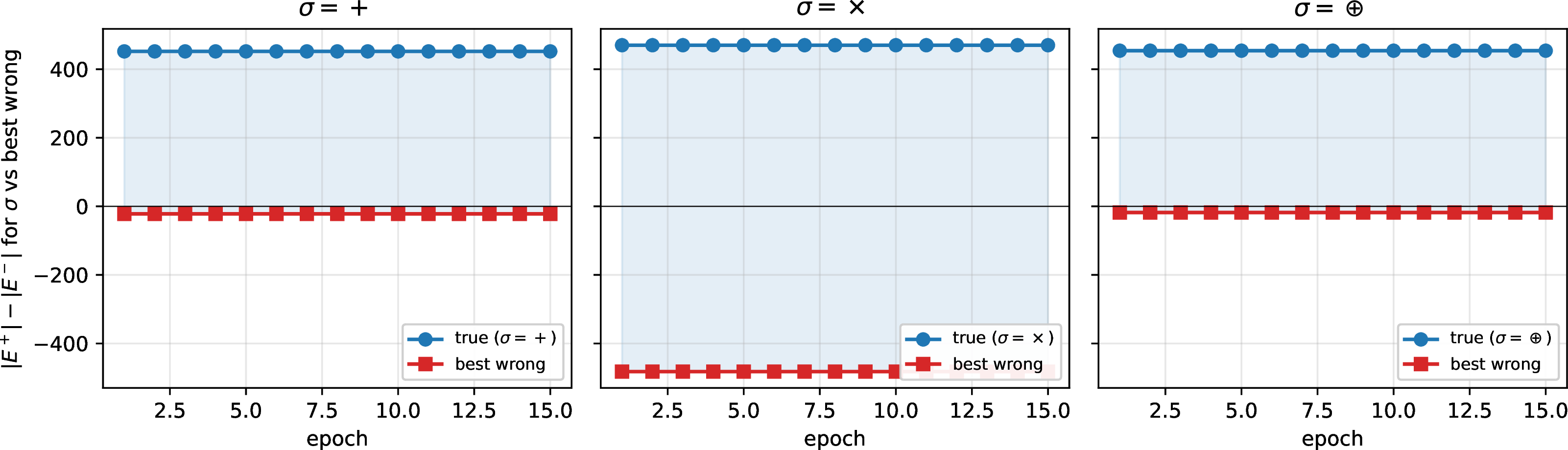
The bag-level loss \(\mathcal{L}_{\text{bag}} = \sum_b -\log \hat{p}_{s_b}\) is a smooth surrogate for the discrete count of bag-level mispredictions. Writing \(E^\pm\) here for the partition induced by the hard bag prediction \(\hat{s}_b = \arg\max_t \hat{p}_t\) of the same distribution \(\hat{p}\) that appears in the loss (appendix B, whose per-bag bound holds for any distribution in \(\Delta(S)\), in particular the mixed \(\hat{p}\)), \(|E^-| \leq \mathcal{L}_{\text{bag}} / \log 2\) as derived below. For a deterministic classifier this partition coincides with the \(\sigma(\mathbf{f}(\mathbf{x})) = s\) partition of §3; for a probabilistic classifier the two can differ, and the Constraint metric of §4a tracks the latter. Proposition 2 establishes that whenever the chosen hard-argmax prediction \(\hat{s}_b\) (under a fixed tie-breaking convention) is incorrect on bag \(b\), \(\hat{p}_{s_b} \leq \tfrac{1}{2}\) and hence \(-\log \hat{p}_{s_b} \geq \log 2\). Summing over bags yields the one-sided inequality \(\mathcal{L}_{\text{bag}} \geq (\log 2)\,|E^-|\), equivalently \(|E^-| \leq \mathcal{L}_{\text{bag}} / \log 2\). Cross-entropy is not monotone in \(|E^-|\) in the other direction: a lower \(\mathcal{L}_{\text{bag}}\) does not imply a lower \(|E^-|\) in general, but minimizing \(\mathcal{L}_{\text{bag}}\) minimizes an upper bound on \(|E^-|\) and, equivalently, maximizes the induced lower bound \(N - 2\mathcal{L}_{\text{bag}}/\log 2\) on \(|E^+| - |E^-| = N - 2|E^-|\). The remaining terms \(\mathcal{L}_{\text{con}}\), \(\mathcal{L}_{\text{cp}}\) and \(\mathcal{L}_{\text{ctp}}\) add structural regularization that encourages the CP-derived and TP-derived bag predictions to agree, without altering this surrogate relationship. The discrete \(|E^+| - |E^-|\) gap is also tractable to track explicitly across training (counting, per candidate operator, the validation bags on which \(\sigma\) applied to the hard per-instance predictions matches \(s_b\)); doing so produces the trajectories of figure 1, in which the true \(\sigma\) is separated from the best competing operator by a large positive gap from epoch 1 onwards (the figure shows all three operators; for \(\sigma = \oplus\) the bag-level separation holds regardless of instance-level collapse, since XOR-equivariant relabellings preserve bag consistency).

4.3 Experiment 1: transition predicate inference from observed predicate and classifier predicate↩︎

This experiment corresponds to scenario 1 in the semantic formulation: inferring the TP given OP and CP. A soft weight vector over the enumerated candidate operators is trained by the four-term loss, and the operator with the largest learned weight is selected (§4a).

To test sensitivity to perceptual reliability, strong CP (a classifier pre-trained in the scenario-2 configuration, i.e.under the true operator, before the operator weights are trained) is compared against random CP (untrained). With strong CP, scenario 1 therefore measures operator identification given a classifier consistent with the true operator; the random-CP condition probes discovery without that assistance. Results are shown in table ¿tbl:tab:exp195tp?. With strong CP, TP inference succeeds for all three operators, achieving 100% operator selection accuracy on every seed and large positive consistency scores. The \(\times\) row reaches reliable operator selection (OpSelAcc \(1.000\)) only after the scenario-1 training configuration is matched to the four-term loss of algorithm 2 (the four-term weights \((\lambda_{\text{bag}}, \lambda_{\text{con}}, \lambda_{\text{cp}}, \lambda_{\text{ctp}}) = (1.0, 1.0, 0.05, 0.5)\), squared \(\ell_2\) distance for \(\mathcal{L}_{\text{ctp}}\), and joint CP–TP optimization rather than the alternating-phase variant); an alternative configuration with non-zero auxiliary entropy and ILP weights left the TP-inference driver in the non-\(1\)-unambiguous multiplicative zero-attractor (appendix C.4) and collapsed operator selection to chance. Under random CP, the consistency signal collapses across all three operators (ConsRatio drops to chance, and ConsScore becomes large and negative). Operator selection behaves differently by operator: for \(+\) and \(\oplus\) the argmax still recovers the true \(\sigma\) (OpSelAcc \(\geq 0.95\)), since the relative ranking of operators survives even when none of the operators fits well, whereas for \(\times\) the multiplicative zero-attractor disrupts even this ranking and OpSelAcc drops to \(0.200 \pm 0.410\). These results show that, in this setup, absolute consistency collapses under random CP, and for \(\times\) even the operator ranking fails; the training configuration also needs to be matched to the operator’s unambiguity profile.

Background-knowledge size

Wang et al.’s theorem 5 [5] is a sample-complexity statement: a larger candidate-operator class \(\mathcal{G}\) increases the number of partially-labelled samples needed to reach a given classification risk, with the dependence captured by the term \(d_{\mathcal{G}}\). Optimization epochs are not the same quantity as sample complexity, so theorem 5 cannot be tested directly with the training-loop measurements. A related empirical trend is reported instead: scenario 1 was run with \(|\Sigma|\) varied from \(1\) (oracle) to \(5\) (true operator plus four distractors, including \(\max\) and \(\min\)). TP identification succeeds with OpSelAcc \(= 1.00\) at every \(|\Sigma|\), with the convergence epoch growing modestly from \(1\) to \(2\) as more candidates are added. This trend is consistent with the qualitative direction of Wang et al.’s theorem 5 [5] (more candidates require more data/effort), without being a formal test of the bound. Full numbers are reported in appendix A.2.

4.4 Experiment 2: classifier predicate inference from observed predicate and fixed transition predicate↩︎

This experiment corresponds to scenario 2: inferring instance-level classifier assignments given OP and a fixed TP. Strong CP (trained under OP constraints) is compared against weak CP (minimally trained: two epochs on 200 bags).

Table ¿tbl:tab:exp295cp? shows that weak CP fails to recover semantic structure on every operator: bag accuracy stalls around \(0.45\)–\(0.50\), a level attributable largely to the OP-candidate component of the evaluation mixture (which places probability \(1/3\) on the true label; §4a) rather than to recovered structure, while constraint satisfaction stays below \(0.22\) and instance accuracy stays below \(0.34\). OP supervision alone is insufficient to recover meaningful instance-level predictions, regardless of the operator. Strong CP, in contrast, achieves bag accuracy and constraint satisfaction of approximately 0.96 on all three operators. Instance accuracy splits along the Wang et al. [5] unambiguity profile (appendix C.2): for the \(M\)-unambiguous operators \(\sigma = +\) and \(\sigma = \times\), instance accuracy reaches 0.97–0.98 in lockstep with bag accuracy. For \(\sigma = \oplus\), which is not \(M\)-unambiguous, instance accuracy is sharply bimodal across the 20 seeds: approximately half of the seeds recover digits with instance accuracy above 0.9 and the other half show instance accuracy near 0 (aggregate \(0.439 \pm 0.497\)) despite preserved bag and constraint accuracy on every seed. This pattern is consistent with collapse to an XOR-equivariant relabelling (mechanism detailed in appendix C.4); the per-seed mapping from confusion matrices is not separately verified, so the verified claim is that the observation is explainable by such a relabelling rather than that each collapsed seed is one. The bimodality is also consistent with the failure mode that Wang et al.’s lemma 1 [5] establishes existentially for non-\(M\)-unambiguous operators (appendix C.4): lemma 1 proves the existence of a data distribution \(\mathcal{D}\) and a classifier with partial risk zero and classification risk one; an XOR-equivariant relabelling would realize this configuration on the actual MNIST distribution rather than on Wang et al.’s [5] adversarial construction.

4.5 Observed predicate quality sensitivity (noise study)↩︎

Robustness to weak supervision quality is analysed by progressively corrupting OP bag labels with increasing levels of noise and evaluating TP inference. In this setting, noise is injected directly into the training OPs (validation labels remain clean), while the underlying instance labels and aggregation rules remain unchanged. TP inference is evaluated using ConsRatio and RatioMargin. ConsRatio measures the fraction of validation bags whose hard CP predictions are consistent with the true operator (§4a); RatioMargin measures the gap to the best competing operator.

All three operators exhibit a plateau in the consistency ratio followed by a sharp transition, but the transition location differs across operators. Addition and XOR maintain ConsRatio above \(0.85\) up to OP-corruption ratio \(0.5\), then drop sharply between \(0.5\) and \(0.7\) before falling to or below chance. By contrast, multiplication stays at or above \(0.83\) up to noise \(0.7\) and drops sharply between \(0.7\) and \(0.8\) (figure 3). The transition in either regime is abrupt rather than gradual, consistent with the bag-level evidence flipping from informative to anti-informative. This behaviour is consistent with the view of weak supervision as a structured logical constraint that the symbolic layer can denoise within the operative regime. The operator-by-operator difference in noise tolerance is consistent with the recent theoretical analysis of Tsamoura et al. [6], which establishes class-specific risk bounds in MI-PLL (their proposition 3.1) that show the symbolic component \(\sigma\) can induce significant per-class learning imbalances even when the hidden-label marginal is uniform. The mechanism Tsamoura et al.identify, namely an asymmetric pre-image distribution under \(\sigma\), is also present for multiplication on the digit range: the bag label \(0\) has an unusually large pre-image because any pair containing a zero maps to \(0\). This makes corrupted labels of that form especially easy for the multiplicative operator to rationalize and provides a plausible structural explanation for the observed noise plateau. Their illustrative \(\sigma = \mathrm{max}\) example exhibits the same general kind of pre-image asymmetry, though in the opposite direction. The multiplication noise plateau is therefore interpreted as empirically related to the pre-image-asymmetry mechanism Tsamoura et al.[6] identify under clean weak-label structure, rather than as a contingent empirical artefact. Tsamoura et al.’s [6] theory does not formally cover OP-corruption regimes, so this is a structural motivation rather than a formal corollary of those bounds. The numerical results for this subsection are reported in appendix A.1, with a detailed mapping to their framework in appendix D.

Scalability and computational cost

The hypothesis space is intentionally restricted to a small operator set in order to isolate semantic dependencies. TP selection requires evaluating candidate hypotheses for consistency, and this introduces overhead compared to purely neural baselines. Runtime scales with the number of bags, the number of candidate operators and the number of constraint instances. This is regarded as the cost of enforcing explicit semantic consistency under weak supervision, and more expressive operator libraries and more search-efficient ILP strategies are left to future work.

Why not an oracle

Unlike an oracle program that hard-codes the true operator, the present setting must infer TP from weak supervision and noisy neural CP outputs; residual errors are therefore expected owing to ambiguity in OP labels and local optima in joint neuro-symbolic optimization.

5 Related work↩︎

The closest theoretical companions to this work are Wang et al. [5] and the recent work of Tsamoura et al. [6]. Wang et al.[5] supply sample-complexity bounds for MI-PLL under unambiguity conditions on the aggregation operator \(\sigma\). Tsamoura et al.[6] extend this analysis to class-specific risk bounds, show that \(\sigma\) can cause per-class learning imbalances even under uniform marginals, and propose linear-programming (LP)-based training-time mitigation together with a robust optimal-transport test-time mitigation algorithm. Their contribution is statistical and algorithmic; appendix D discusses how those imbalance-mitigation techniques compose with the present framework.

Several neuro-symbolic frameworks combine logic with neural learning to handle structured supervision: Scallop [13], DeepProbLog [14], [15] (built on Sato’s distribution semantics [16]), DeepStochLog [17], NeurASP [18], NeuroLog [19], SATNet [20], logic tensor networks [21], logical neural networks [22], neural theorem provers [23], \(\partial\)Forth [24], semantic loss [25], DL2 [26], abductive learning [27], neural-guided program synthesis [28] and related variants [29], [30]. These systems integrate symbolic constraints through different mechanisms (probabilistic logic programs, soft satisfaction and abduction). The experimental pipeline here follows the differentiable-ILP design of \(\alpha\)-ILP [12], representing neural predicates and scoring symbolic hypotheses by differentiable consistency.

Single-instance partial label learning has been studied extensively [31]–[39], including transition-matrix-based analyses for noisy supervision [40]–[43]; this work targets the multi-instance setting [44]–[46], where bag-level supervision aggregates latent instance labels; multi-instance learning is reviewed by Foulds &Frank [47], with theoretical learnability bounds for bag-level supervision developed by Sabato et al.[48]. Learning from label proportions [49], [50] is a related bag-level weak-supervision paradigm in which bags carry class-proportion annotations rather than operator-aggregated labels. Other approaches to weak supervision include relaxed supervision [51], structured prediction with paired examples [52]–[56] and combinatorial solvers integrated into neural architectures [57], [58]. Weak supervision in natural language processing [59], [60] is a separate major line focused on text-domain structure.

6 Discussion↩︎

The CP/TP/OP-coupled model consistently outperforms the no-CP, no-TP and OP-only ablations across operators (table ¿tbl:tab:unified95ablation?), indicating that structured symbolic guidance both improves bag-level prediction and reveals semantic failure modes that bag accuracy alone would hide.

At the theoretical level, this work builds on Wang et al. [5], whose theorem 5 establishes empirical-risk-minimization learnability under an unknown transition class \(\mathcal{G}\), conditional on the unambiguity of \(\mathcal{G}\) (definition 5 there) and the \(r\)-bounded assumption: every classifier \(f\) in the search space \(\mathcal{F}\) satisfies the class-conditional accuracy lower bound \(\mathbb{P}([f](X) = y \mid Y = y) \geq r\) for some \(r > 0\) and every label \(y \in Y\). The empirical observation that TP discovery (scenario 1) requires a competent CP, documented in the strong-CP versus random-CP comparison of experiment 1 (table ¿tbl:tab:exp195tp?), is consistent with this condition: a cold-start CP has near-random hard predictions \([f](x)\), so the class-conditional hard accuracy \(\mathbb{P}([f](X) = y \mid Y = y)\) can be near chance (in expectation \(\approx 1/c\), where \(c = 10\) is the number of digit classes, under symmetric random initialization) or even zero on some classes that the cold-start argmax happens to never output; the zero case falls below every positive \(r\), and the near-chance case below any \(r\) exceeding \(1/c\), so the \(r\)-bounded premise fails at the strengths the learnability bounds need. Scenario-2 pre-training lifts the pre-trained CP’s class-conditional hard accuracy above \(1/c\) on non-collapsed seeds, giving an empirical analogue of Wang et al.’s [5] \(r\)-bounded condition for the specific CP that is then used. The \(r\)-bounded assumption is a property of the entire search class \(\mathcal{F}\), not of an individual classifier, so this correspondence is operational rather than a literal class-level verification. The same observation has a sharper reading under the class-specific risk framework of Tsamoura et al. [6]: a cold-start CP also has near-trivial partial risk \(\mathcal{R}^{01}_{\textsf{P}}(f; \sigma) \approx 1\), at which Tsamoura et al.’s [6] class-specific bound \(\Phi_{\sigma, j}\) (Tsamoura et al.’s proposition 3.1; growth curves shown in Tsamoura et al.’s figure 2) is uninformative: by construction \(\Phi_{\sigma, j}(R_{\textsf{P}}) \leq 1\), matching the trivial bound \(R_j(f) \leq 1\) on every class. Scenario-2 pre-training lowers the partial risk into the regime where the bound becomes non-trivial and recovers a per-class profile that TP discovery can use to distinguish candidate operators. The formal mappings are detailed in appendices C and D.

The present work builds on recent advances in differentiable ILP, including the foundational \(\partial\)ILP system of Evans &Grefenstette [61] and the \(\alpha\)-ILP system [12], which integrates logical clause learning with neural perception predicates. Extensions such as Shindo et al. [62], Sen et al. [22], Krishnan et al. [63] and Gao et al. [64] have expanded this line of research by enabling clause-level control, supporting first-order logic, and introducing predicate invention and recursive rule learning. However, a formal semantics for MI-PLL within such systems remains underdeveloped. The semantics formalization here provides one step towards filling that gap by making explicit the structural assumptions that ILP systems can exploit in MI-PLL settings.

Three challenges remain for future work. Cross-domain robustness requires the framework’s behaviour to remain consistent across variations in image representations, which can vary significantly across datasets. The expressivity of the transition logic is constrained: both scenarios assume a finite candidate set of symbolic aggregation operators, and the dependence on hand-engineered background knowledge limits adaptability; extending ILP to support flexible rule discovery and learned background knowledge would broaden the framework beyond the current candidate operator set. Delayed supervision is another challenge: the current formulation assumes that OP labels are immediately available for every bag, whereas many practical settings provide feedback that is delayed or only conditionally available, requiring extension to time-indexed or deferred logical feedback in OP.

The approach does not modify the classifier’s architecture; the symbolic constraints are introduced through the loss function during training. The framework also enables diagnostic comparisons between the classifier’s outputs and the ILP-derived consistent predictions, which can expose semantic failure modes such as reasoning shortcuts [65], [66]. The gap metrics reported in §4 (Bag–Constraint and Bag–Inst) operationalize this kind of diagnostic check.

Although this paper addresses only two specific scenarios, TP inference given an available CP and CP inference given a fixed TP, these provide a starting point for a broader ILP-based treatment of MI-PLL. Future work will generalize this to cases with latent or partially known predicates, explore more complex supervision structures and expand empirical testing across diverse datasets. A direct extension is to compose the CP/TP/OP semantics with the class-specific imbalance-mitigation algorithms of Tsamoura et al. [6]: the marginal-estimation procedure, LP pseudolabel assignment and the CAROT test-time score adjustment (confidence adjustment via robust semi-constrained optimal transport) plug into the CP layer and could be used to address the XOR bimodal seed-collapse, and the post-plateau collapse in multiplication under OP noise. The mapping is detailed in appendix D.

7 Conclusion↩︎

This paper introduced a semantic framework for MI-PLLbased on three auxiliary predicates: the CP, the TP and the OP. Two inductive tasks were formalized within this framework, inferring TP given an available CP and inferring CP given a fixed TP, and the framework was evaluated using an \(\alpha\)-ILP-style differentiable pipeline as the backend on MI-PLL tasks constructed from MNIST. Across the operators \(+\), \(\times\) and \(\oplus\), the experiments expose operator-dependent failure modes that bag accuracy alone would hide, in line with the unambiguity conditions of Wang et al.[5] and the class-specific risk framework of Tsamoura et al. [6]. Extending the framework to larger operator libraries, delayed supervision and direct integration with class-specific mitigation algorithms remains future work.

Data accessibility

This article has no additional data. The code that supports the findings is available at https://github.com/nuuoe/ILP_MI-PLL.

Appendix A. Additional experimental results↩︎

7.1 Observed predicate noise sensitivity↩︎

Table ¿tbl:tab:op95noise? reports the full per-noise-level TP inference results that underlie the OP-noise discussion in §4. Results are shown as mean \(\pm\) standard deviation over 10 seeds, with the scenario-1 training configuration matched to the algorithm 2 four-term loss. All three operators exhibit a plateau-then-cliff pattern: addition and XOR transition between noise \(0.5\) and \(0.7\), while multiplication transitions between \(0.7\) and \(0.8\). The clean-label sample-complexity bounds of Wang et al.[5] do not directly model OP corruption and therefore do not predict this asymmetry in the transition location; a structural interpretation in terms of Tsamoura et al.’s [6] class-specific framework (which is a clean-weak-label theory under known \(\sigma\), not an OP-noise theory) is given in appendix D.

7.2 Background-knowledge size↩︎

To probe the effect of background-knowledge size \(|B|\) on TP discovery empirically, scenario 1 was run with the candidate-operator set \(\Sigma\) varied from \(|\Sigma| = 1\) (only the true operator) to \(|\Sigma| = 5\) (the set \(\{+, \times, \oplus, \max, \min\}\), which contains the true operator); \(|B|\) is measured here by \(|\Sigma|\), the number of candidate operators the background theory encodes. This corresponds operationally to varying \(d_{\mathcal{G}}\) in theorem 5 of Wang et al.[5] (appendix C.6). Results, averaged over 10 seeds, are reported in table ¿tbl:tab:bk95sweep?. OpSelAcc is as in §4a; ConvRate is the fraction of seeds whose true-operator weight exceeds \(0.9\) during training; ConvEp is the first epoch at which this occurs; margin denotes the operator-weight margin \(w_{\sigma_{\text{true}}} - \max_{\sigma \neq \sigma_{\text{true}}} w_\sigma\) of the learned operator weights at the final epoch (at \(|B| = 1\) the competitor set is empty and the margin is defined as \(w_{\sigma_{\text{true}}}\)).

Operator-selection accuracy holds at 1.00 across \(|B| \in \{1, \ldots, 5\}\) for all three operators, confirming that TP identification succeeds under strong CP for every candidate-set size in this range. The convergence epoch grows from 1.0 at \(|B| = 1\) to approximately 2.0 at \(|B| \geq 3\) for \(+\) and \(\oplus\), and similarly for \(\times\) (with a slightly slower transition at \(|B| = 3\), mean \(1.7 \pm 0.5\), indicating that some seeds still converge in one epoch at \(|B| = 3\)). Enlarging the candidate set does not change the final operator selection in any of the runs. This is read as the empirical analogue of the qualitative direction of Wang et al.’s theorem 5: smaller \(\mathcal{G}\) yields smaller sample complexity in their setting, and smaller optimization-epoch counts are observed here. The two quantities (theorem 5’s \(m_{\textsf{P}}\) and the epoch count) are not the same; the convergence-epoch trend is a related empirical signal, not a formal test of the bound.

Appendix B. Formal statements and proofs↩︎

This appendix restates, with explicit assumptions, the load-bearing arithmetic and combinatorial claims made throughout the main text and provides concise proofs.

Setting and notation

Fix a finite label set \(Y\), an instance space \(X\), a bag size \(M \geq 1\) and a finite bag-label space \(S\). The true aggregation rule \(\sigma \colon Y^M \to S\) and the latent data-generating process \(D \colon X^M \to S\) are total functions related by \(D(\mathbf{x}) = \sigma(g(x_1), \ldots, g(x_M))\), where \(g \colon X \to Y\) is the (latent) per-instance gold-label map; throughout the appendix, \(s^{(b)} = D(\mathbf{x}^{(b)})\) denotes the observed bag label without reference to the latent factorization. A weakly-labelled dataset is a finite list \(\mathcal{D} = ((\mathbf{x}^{(b)}, s^{(b)}))_{b=1}^{N}\) with \(\mathbf{x}^{(b)} \in X^M\) and \(s^{(b)} = D(\mathbf{x}^{(b)})\). A hypothesis is a pair \(H = (f, \sigma)\), where \(\sigma \colon Y^M \to S\) is drawn from a finite candidate set \(\Sigma\), and \(f\) is either a deterministic classifier \(X \to Y\) or, more generally, a probabilistic classifier \(\tilde{f} \colon X \to \Delta(Y)\), where \(\Delta(Y)\) is the probability simplex over \(Y\).

Every hypothesis induces a soft bag distribution \(\hat{p}(H, \mathbf{x}) \in \Delta(S)\) by marginalizing the operator \(\sigma\) over the per-instance distributions: \[\hat{p}(H, \mathbf{x})_t \;=\; \sum_{\mathbf{y} \in Y^M,\; \sigma(\mathbf{y}) = t} \prod_{i=1}^{M} \tilde{f}(x_i)_{y_i}, \qquad t \in S.\] The associated hard prediction is \(\hat{s}(H, \mathbf{x}) := \arg\max_{t \in S} \hat{p}(H, \mathbf{x})_t\), with ties broken by any fixed rule. For a deterministic classifier, \(\tilde{f}\) is a Dirac mass and \(\hat{p}(H, \mathbf{x})\) reduces to a Dirac at \(\sigma(f(x_1), \ldots, f(x_M))\). For a probabilistic classifier, the argmax-of-marginal prediction used here need not coincide with \(\sigma\) applied to the per-instance argmaxes (the Constraint metric of §4a); proposition 2 concerns the former, i.e.the bag-level prediction scored by \(\mathcal{L}_{\mathrm{bag}}\). Define the hypothesis-dependent partition \[E^+(H) \;=\; \{(\mathbf{x}, s) \in \mathcal{D} \,:\, \hat{s}(H, \mathbf{x}) = s\}\text{ and} \qquad E^-(H) \;=\; \{(\mathbf{x}, s) \in \mathcal{D} \,:\, \hat{s}(H, \mathbf{x}) \neq s\}.\] Bags are assumed pairwise distinct, so the two sets partition \(\mathcal{D}\); equivalently, \(E^\pm(H)\) may be read as index sets over \(\{1, \ldots, N\}\). The standard information-theoretic conventions \(0 \log 0 = 0\) and \(-\log 0 = +\infty\) are adopted.

Notation conventions used throughout the main text

The worked examples and formal statements use the following two conventions throughout:

1. Sample form for training data. A training example with bag \((x_1, \ldots, x_M)\) and observed weak label \(s\) is written compactly as the tuple \((x_1, \ldots, x_M, s)\); this is the same datum that the atom \(\text{OP}((x_1, \ldots, x_M), s)\) records. Sample form is used when enumerating training data; the formal predicate form is used inside constraint structures, theorem statements and proofs.

2. Operator subscripts. The \(\text{TP}\), the intermediate-interpretation structure \(\mathbb{I}\) and the hypothesis \(\mathbb{H}\) all carry a subscript indicating the aggregation operator. When the operator is fixed and given as part of the problem setup (as in scenario 2 of §3, where \(\sigma\) is provided), the symbol is written directly: \(\text{TP}_+, \text{TP}_\times, \text{TP}_\oplus, \text{TP}_C\), and likewise \(\mathbb{I}_+, \mathbb{I}_\times, \mathbb{I}_\oplus, \mathbb{I}_C\) and \(\mathbb{H}_+, \mathbb{H}_\times, \mathbb{H}_\oplus, \mathbb{H}_C\). When the operator is hypothesized, generic, unknown or being searched over (as in scenario 1, where \(\sigma\) is inferred), \(\text{TP}_\sigma\), \(\mathbb{I}_\sigma\) and \(\mathbb{H}_\sigma\) are written.

Remark (mixture instantiation)

The per-bag inequality of proposition 2 holds for any \(p \in \Delta(S)\), so the dataset-level bound applies verbatim when each bag’s distribution is the mixed \(\hat{p}\) of algorithm 2 rather than the pure CP-marginal \(\hat{p}(H, \mathbf{x})\) defined above, with \(E^\pm(H)\) read as the partition induced by the argmax of that same mixed distribution.

Remarks on usage in the main text

Lemma 1 and proposition 1 jointly formalize the abductive-partition remark of §3 and provide the precise sense in which the stated ILP objective reduces to bag-level classification accuracy under the \((f, \sigma)\) decomposition. Proposition 2 justifies the surrogate-relationship paragraph in §4: minimizing the soft bag-level cross-entropy minimizes an upper bound on the discrete misclassification count \(|E^-|\); explicitly, \(|E^-| \leq \mathcal{L}_{\text{bag}} / \log 2\). Lemma 2 confirms the partial permutation-invariance caveat in §3b. Lemma 3 makes precise the structural ambiguity of \(\sigma = \oplus\) on the digit range: every feasible XOR bag label has at least two distinct instance-pair pre-images, in line with the empirical observation that no bag label has a unique pre-image on \(Y\).

Appendix C. Mapping to learnability theory↩︎

The present paper builds on the multi-instance partial label learnability framework of Wang et al.[5]. This appendix supplies the precise mapping between Wang et al.’s [5] formal apparatus and the CP/TP/OP semantics developed in the main text. The relevant theorems are restated, the unambiguity conditions are verified for each operator used in the experiments, the empirical interpretations supported are spelled out, and what the ILP-based extension adds on top of these results is made explicit.

7.3 Notation↩︎

Wang et al.[5] study MI-PLL: pairs \((\mathbf{x}, s)\) with hidden instance-label vectors \(\mathbf{y}\) such that \(s = \sigma(\mathbf{y})\). Throughout the appendices, \(c := |\mathcal{Y}|\) denotes the number of instance classes (\(c = 10\) in the experiments; \(\mathcal{Y}\) is the instance label set written \(Y\) in the main text). That formal machinery is statistical: the analysis works with VC and Natarajan dimensions of induced classifier families, Rademacher complexity of scoring classes (standard treatments are given in [67]), partial-risk notation \(\mathcal{R}^{01}_{\textsf{P}}(f;\sigma)\) and the empirical counterpart \(\widehat{\mathcal{R}}^{01}_{\textsf{P}}(f;\sigma;\mathcal{T}_{\textsf{P}})\) and weighted-model-count semantic losses. Carrying all of this notation into the body of this paper would substantially increase the notational burden without changing the predicate-level decomposition presented here: this predicate-level decomposition (CP, TP and OP) operates at the logical level where statistical-learning constants do not normally appear. A deliberately lighter notation is therefore used in the main text, writing \(E^+(H)\text{ and }E^-(H)\) for the partition and \(\mathcal{L}_{\text{bag}}\) for the bag-level surrogate, and confining Wang et al.’s [5] full statistical apparatus to this appendix, where it is needed for the formal claims. The correspondence is as follows.

5pt

7.4 Unambiguity conditions↩︎

The two conditions relied on are those introduced by Wang et al. [5].

For \(M = 2\) (the bag size in the experiments) and \(\mathcal{Y} = \{0, 1, \ldots, 9\}\), it is now verified which of the operators satisfy each condition.

7.5 Main learnability theorems↩︎

The two learnability results from Wang et al. [5] relied on are restated here, using the simplified notation of appendix C.1.

Combining proposition 3 above with propositions 4 and 5 of Wang et al. [5] yields the following corollary, which is the form in which these results are used.

7.6 Implications for the empirical observations↩︎

Corollary 1 gives a sample-complexity regime for each operator (fast for \(+\), slow \(M\)-th-root for \(\times\) and existential non-learnability for \(\oplus\)). These regimes predict no gradient-descent dynamics and serve only to interpret the empirical behaviour reported in §4, in the sense that the observations are consistent with the regime each operator falls into.

(i) Addition trains cleanly

The fast rate \(\widetilde{\mathcal{O}}(1/\epsilon)\) of proposition 5 for \(\sigma = +\) is consistent with the convergence of the \(+\) scenario-2 runs in 15 epochs to mean bag accuracy 0.96 and mean instance accuracy 0.98 over the 20 seeds (per-seed minima 0.93 and 0.97, respectively).

(ii) Multiplication requires careful loss balancing

The non-\(1\)-unambiguity of \(\times\) (proposition 3 case 2) is the formal condition associated with the multiplicative zero-attractor observed. Working at the level of the soft outer product \(P_s = \sum_{(a, b) \in Y \times Y \,:\, a \cdot b = s} \text{cp}_1[a]\,\text{cp}_2[b]\) (the categorical bag-marginal of appendix C.5), for every \(s > 0\) and every \(a > 0\), \[\partial P_s / \partial \text{cp}_1[a] \;=\; \mathbf{1}\{a \mid s,\;s/a \in Y\} \cdot \text{cp}_2[s/a],\] so at \(\text{cp}_2 = \delta_0\), the entire Jacobian \(\partial P_s / \partial \text{cp}_1[\,\cdot\,]\) is zero for every \(s > 0\), and \(P_s\) is zero there. The log-form loss \(-\log P_s\) (the bag cross-entropy \(\mathcal{L}_{\text{bag}}\) in the pure-CP configuration \(w_{\text{CP}} = 1\) of appendix C.5) is singular at the boundary \(P_s = 0\); the gradient of \(-\log P_s\) is a \(0/0\) form near the attractor, and no claim is made that it is small there (indeed along the joint perturbation \(\text{cp}_1 = \text{cp}_2 = (1-\eta,\eta/(c-1),\ldots,\eta/(c-1))\) its magnitude grows as \(\Theta(1/\eta)\) for small \(\eta\)). The analytic fact relied on is the categorical-marginal one: \(P_s\) and the Jacobian \(\partial P_s / \partial \text{cp}_1\) both saturate towards zero at \(\text{cp}_1 = \text{cp}_2 = \delta_0\) for every \(s > 0\) and remain small in a neighbourhood, so the probability mass that the constraint loss can move out of the attractor is small there. This probability-mass saturation, together with the log-loss singularity at \(P_s = 0\), is why \(\sigma = \times\) is sensitive to loss balancing: as documented in §4 (experiment 1), the four-term loss with auxiliary entropy and ILP-style regularizers disabled (\(\lambda_{\text{ent}} = \lambda_{\text{ilp}} = 0\)) avoids the attractor, while adding those auxiliaries with non-zero weights (\(\lambda_{\text{ent}} = 0.15\text{ and } \lambda_{\text{ilp}} = 0.5\)) drives the optimizer into it. Proposition 4 of Wang et al.[5] guarantees that learning is still possible, but only at the slower \(M\)-th-root sample-complexity rate. The theorem is a sample-complexity statement and does not predict gradient-descent dynamics; the empirical observation of higher per-seed variance and the practical need for a carefully balanced loss (the four-term configuration of algorithm 2 with weights \((\lambda_{\text{bag}}, \lambda_{\text{con}}, \lambda_{\text{cp}}, \lambda_{\text{ctp}}) = (1.0, 1.0, 0.05, 0.5)\), rather than an alternative variant with \(\lambda_{\text{ent}} = 0.15, \lambda_{\text{ilp}} = 0.5\)) is consistent with the slower-rate regime predicted by proposition 4, as reported in §4.

(iii) XOR exhibits the non-\(M\)-unambiguous failure mode

The XOR scenario-2 runs achieve bag accuracy and constraint satisfaction both approximately \(0.96\) across all 20 seeds, but display a bimodal instance accuracy: roughly half of the seeds converge to instance accuracy above \(0.9\), and the remaining seeds collapse to instance accuracy near \(0\), yielding the aggregate \(0.439 \pm 0.497\) reported in table ¿tbl:tab:exp295cp?. A canonical mechanism explaining this pattern is an XOR-equivariant relabelling: any classifier \(\tilde{f}\) satisfying \(\tilde{f}(x_1) \oplus \tilde{f}(x_2) = y_1 \oplus y_2 = s\) on every bag preserves bag accuracy and constraint satisfaction regardless of how it maps individual instances. The canonical parametrized family is \(\tilde{f}(x) = y(x) \oplus \kappa\) for a fixed constant \(\kappa\) that is label-preserving on the digit range \(\mathcal{Y} = \{0, \ldots, 9\}\), i.e. \(y \oplus \kappa \in \mathcal{Y}\) for every \(y \in \mathcal{Y}\); the only such \(\kappa\) are \(0\) and \(1\) (any larger \(\kappa\) takes some digit out of \(\mathcal{Y}\)). On this family, \((y_1 \oplus \kappa) \oplus (y_2 \oplus \kappa) = y_1 \oplus y_2 = s\), so bag and constraint accuracy are preserved; instance accuracy is correct at \(\kappa = 0\) and zero at \(\kappa = 1\). The \(\kappa = 1\) realization is the parity flip \(0 \leftrightarrow 1, 2 \leftrightarrow 3, \ldots, 8 \leftrightarrow 9\). The collapsed seeds are characterized through this family at the level of the bag identity it satisfies; the seed-level confusion matrix is not separately inspected to identify which specific relabelling each collapsed seed realizes.

This pattern is consistent with the existential failure mode captured by Wang et al.’s lemma 1 [5]: the lemma proves the existence of a data distribution and a classifier \(f\) with \(\mathcal{R}^{01}_{\textsf{P}}(f; \oplus) = 0\) yet \(\mathcal{R}^{01}(f) = 1\). Any non-trivial XOR-equivariant relabelling \(\tilde{f}(x) = y(x) \oplus \kappa\) with \(\kappa \neq 0\) would realize this configuration on the actual MNIST distribution: partial risk is zero because every bag XOR is preserved, and instance risk is one because every instance label is wrong. The connection to lemma 1 is that both phenomena exploit the non-\(M\)-unambiguity of \(\oplus\) (the diagonal-vector collapse \(\oplus(y, y) = 0\) implies that XOR-equivariant relabellings form a non-trivial isotropy group for \(\sigma\)); the formal statement is existential, and the empirical observation is consistent with a gradient-descent attractor in that isotropy group. The class-specific bound of Tsamoura et al. [6] (proposition 3.1) permits the uniform-bad per-class attainment that such a relabelling would realize, without predicting it; the point is developed in appendix D.4.

7.7 Top-\(k\) surrogate and bag-level cross-entropy↩︎

Wang et al.[5] def. 3 introduces the top-\(k\) partial loss \[\ell^k_\sigma(f(\mathbf{x}), s) \;:=\; \mathrm{SL}\Bigl(\bigvee_{i = 1}^{k} \mathbf{y}^{(i)},\; f(\mathbf{x})\Bigr), \label{eq:wang-topk}\tag{3}\] where \(\mathbf{y}^{(1)}, \ldots, \mathbf{y}^{(k)}\) are the top-\(k\) maximizers of \(P_{f(\mathbf{x})}(\mathbf{y}) := \prod_i \tilde{f}(x_i)_{y_i}\) in the pre-image \(\sigma^{-1}(s)\), and \(\mathrm{SL}\) is the semantic loss (negative log weighted-model-count).

For \(k = |\sigma^{-1}(s)|\), the disjunction is a positive DNF (Disjunctive Normal Form) formula over Boolean variables \(A_{i, y}\) (true iff instance \(i\) is assigned label \(y\)). In Wang et al.’s [5] WMC semantics, the Boolean variables are a priori independent, so different label-vector conjunctions \(\boldsymbol{\Phi}_{\mathbf{y}^{(i)}}\) and \(\boldsymbol{\Phi}_{\mathbf{y}^{(j)}}\) can be simultaneously satisfied by Boolean interpretations that assign each instance multiple labels. Adding an exclusiveness constraint \(\Xi\) of the form \(\neg(A_{i, y} \wedge A_{i, y'})\) for every \(i\) and every \(y \neq y'\) reduces the model count by suppressing those multi-label interpretations (Wang et al. [5] §A.1, discussion following lemma 2).

The framework here instead uses a categorical model directly: each \(\tilde{f}(x_i)\) is a softmax over \(Y\) summing to one. The quantity \(\sum_{\mathbf{y} \in \sigma^{-1}(s)} \prod_i \tilde{f}(x_i)_{y_i}\) computed as the soft outer product is the marginal probability \(\mathbb{P}(\sigma(\mathbf{y}) = s)\) under independent categorical draws \(y_i \sim \tilde{f}(x_i)\). This is treated as a categorical analogue of Wang et al.’s [5] WMC: the two objects sum over the same set of witnessing label-vector assignments in the pre-image, but the underlying probabilistic semantics are different (Wang et al.’s [5] WMC sums over independent-Bernoulli interpretations, each contributing both true-variable factors \(\omega(A_{i,y})\) and false-variable factors \(1 - \omega(A_{i,y'})\); the categorical product has no false-variable factors). The two formulas are not identical in general and coincide only on degenerate inputs (e.g. one-hot \(\tilde{f}(x_i)\)). The categorical form is used throughout because it is the standard output of a neural classifier.

Under this categorical reading, when the bag prediction \(\hat{s}(H, \mathbf{x})\) is computed purely from CP through the soft outer product (algorithm 2 mixing weights \(w_{\text{CP}} = 1\text{ and } w_{\text{OP}} = w_{\text{TP}} = 0\)), the bag-level cross-entropy loss \(\mathcal{L}_{\text{bag}} = -\log \hat{p}(H, \mathbf{x})[s]\) takes the form \(-\log \sum_{\mathbf{y} \in \sigma^{-1}(s)} \prod_i \tilde{f}(x_i)_{y_i}\), i.e.the categorical-marginal counterpart of Wang et al.’s [5] full-pre-image top-\(k\) loss for \(k = |\sigma^{-1}(s)|\). For the more general case \(w_{\text{CP}} \in (0, 1)\), the combined bag prediction \(\hat{p}\) mixes \(\hat{p}_{\text{CP}}\) with \(p_{\text{OP}}\) and \(\hat{p}_{\text{TP}}\); only the \(\hat{p}_{\text{CP}}\) component is the categorical analogue of Wang et al.’s [5] top-\(k\)/WMC family. Wang et al.’s theorem 2 [5] is stated for the WMC/top-\(k\) loss with Bernoulli-variable semantics; it is not stated for the categorical bag cross-entropy here, and no Rademacher argument is provided that rederives the bound for the categorical surrogate. The implication drawn below is therefore by analogy with Wang et al.’s [5] formal result rather than as a direct corollary; the mixed training objective of algorithm 2, with the additional structural terms \(\mathcal{L}_{\text{con}}, \mathcal{L}_{\text{cp}}\text{ and } \mathcal{L}_{\text{ctp}}\), is an empirical extension that no Wang et al.[5] bound covers in either literal or analogue form.

Theorem 2 of Wang et al.[5] requires \(\sigma\) to be both \(1\)- and \(M\)-unambiguous, and yields, for any integer \(k \geq 1\) and \(\delta \in (0, 1)\), with probability at least \(1 - \delta\), the following Rademacher-style bound on the classification risk: \[\mathcal{R}^{01}(f) \;\leq\; \Phi\!\left( (k + 1)\,\left( \widehat{\mathcal{R}}^{k}_{\textsf{P}}(f; \sigma; \mathcal{T}_{\textsf{P}}) + 2\sqrt{2 k}\, M^{3/2} \mathfrak{R}_{M m_{\textsf{P}}}(\mathcal{F}) + \sqrt{\tfrac{\log(1/\delta)}{2 m_{\textsf{P}}}}\right)\right), \label{eq:wang-thm2-bound}\tag{4}\] where \(\Phi\) is an increasing function with \(\Phi(t)/t \to 1\) as \(t \to 0\), and \(\mathfrak{R}_m(\mathcal{F})\) denotes the Rademacher complexity of the scoring class \(\mathcal{F}\) [68]. By proposition 3, the joint \(1\)- and \(M\)-unambiguity requirement is satisfied only by \(\sigma = +\) among the operators studied here; \(\sigma = \times\) is covered only by proposition 4’s slower \(M\)-unambiguous rate, and \(\sigma = \oplus\) is not covered by either aggregate Wang et al.[5] bound. When the bag prediction is computed from CP through the soft outer product with \(k = |\sigma^{-1}(s)|\) (equivalently, the algorithm 2 configuration \(w_{\text{CP}} = 1\text{ and } w_{\text{OP}} = w_{\text{TP}} = 0\)), the bag-CE term \(\mathcal{L}_{\text{bag}}\) is the categorical analogue of Wang et al.’s [5] full-pre-image top-\(k\) loss. For \(\sigma = +\), which is both \(1\)- and \(M\)-unambiguous, eqn (4 ) as stated applies to Wang et al.’s [5] WMC/top-\(k\) surrogate; it is used only as an analogue for the categorical bag-CE, since no separate Rademacher derivation is given here that would extend the bound literally to \(\mathcal{L}_{\text{bag}}\). With that analogue reading, the bound gives a high-probability upper bound on the classification risk \(\mathcal{R}^{01}(f)\) in terms of the empirical top-\(k\) risk and a Rademacher-plus-Hoeffding deviation term, and complements the deterministic proposition 2. The bound is conditional in the standard sense (a small empirical top-\(k\) risk plus a small deviation term yields a small \(\mathcal{R}^{01}(f)\)), and does not guarantee that gradient descent achieves the small-empirical-risk precondition. Proposition 2 provides the complementary deterministic statement \(|E^-| \leq \mathcal{L}_{\text{bag}} / \log 2\), so \(\mathcal{L}_{\text{bag}} / \log 2\) upper-bounds the discrete misclassification count.

Note that the \(E^+/E^-\) tracking routine is a tracking-only utility, used to produce the per-epoch hard partition counts of figure 1 (\(\sigma\) applied to the hard per-instance predictions, counted against \(s_b\) on the validation set, per candidate operator); it does not contribute to the training loss. A separate linear-surrogate loss \(1 - \hat{p}(H, \mathbf{x})[s]\), monotone-related to the log-form top-\(k\) loss of Wang et al.[5] but not formally identical, exists in the implementation and is disabled (weight zero) in all reported runs. The training loss used throughout the experiments is the four-term \(\mathcal{L}_{\text{bag}} + \lambda_{\text{con}} \mathcal{L}_{\text{con}} + \lambda_{\text{cp}} \mathcal{L}_{\text{cp}} + \lambda_{\text{ctp}} \mathcal{L}_{\text{ctp}}\) of algorithm 2; only the bag-CE component \(\mathcal{L}_{\text{bag}}\) is the component analogous to the Wang et al.top-\(k\)/WMC family in eqn (4 ). The three structural terms \(\mathcal{L}_{\text{con}}, \mathcal{L}_{\text{cp}}\text{ and } \mathcal{L}_{\text{ctp}}\) provide additional inductive bias on top of that surrogate; bounding the population risk under the full four-term loss would require a separate Rademacher argument and is beyond the scope of this paper.

7.8 Background knowledge and unknown transitions↩︎

When \(\sigma\) is unknown, Wang et al.[5] consider a transition class \(\mathcal{G}\) of candidate transitions including the true one. Wang et al.’s def. 5 introduces the unambiguity of \(\mathcal{G}\) condition: for each \(\sigma' \in \mathcal{G}\), each diagonal label vector \(\mathbf{y} = (l_i, \ldots, l_i)\) and each label \(l_j \neq l_i\), some vector \(\mathbf{y}' \in \{l_i, l_j\}^M\) satisfies \(\sigma'(\mathbf{y}') \neq \sigma(\mathbf{y})\), where \(\sigma\) is the true transition. A scoring class \(\mathcal{F}\) is \(r\)-bounded (Wang et al.’s §5) if there exists \(r > 0\) such that \(\mathbb{P}(\,[f](X) = y \mid Y = y\,) \geq r\) for every \(y \in \mathcal{Y}\) and every \(f \in \mathcal{F}\); i.e. every classifier in the search space has class-conditional hard-prediction accuracy at least \(r\) on every class. Under the unambiguity of \(\mathcal{G}\) and the \(r\)-boundedness of \(\mathcal{F}\), theorem 5 of Wang et al. [5] establishes \(\mathcal{R}^{01}(f) \leq \mathcal{O}(\mathcal{R}^{01}_{\textsf{P}}(f; \mathcal{G})^{1/M})\) as \(\mathcal{R}^{01}_{\textsf{P}}(f; \mathcal{G}) \to 0\), with sample complexity \[\begin{align} m_{\textsf{P}} \geq{} & C_4 \cdot \frac{c^{2M-2}}{r^M \epsilon^M} \\ & \cdot \Bigl(\bigl((d_{[\mathcal{F}]} + d_{\mathcal{G}})\log(6M(d_{[\mathcal{F}]} + d_{\mathcal{G}})) + d_{[\mathcal{F}]}\log c\bigr) \\ & \quad \cdot \log\!\bigl(c^{2M-2}/(r^M \epsilon^M)\bigr) + \log(1/\delta)\Bigr). \end{align}\] The key new term is \(d_{\mathcal{G}}\), the VC dimension of the family of indicator functions \(\{(\mathbf{y}, s) \mapsto \mathbb{1}\{\sigma'(\mathbf{y}) \neq s\} : \sigma' \in \mathcal{G}\}\). The background-knowledge size study experiment, in which the candidate-operator set \(\Sigma\), the ILP-style realization of Wang et al.’s [5] transition class \(\mathcal{G}\), is varied from \(|\Sigma| = 1\) to \(|\Sigma| = 5\), corresponds operationally to varying \(d_{\mathcal{G}}\). The monotonic increase in convergence epoch reported here (appendix A.2, table ¿tbl:tab:bk95sweep?) is the empirical analogue of the qualitative direction of Wang et al.’s theorem 5[5]: the bound is on sample complexity \(m_{\textsf{P}}\) and the quantity here is on optimization epochs, so the two quantities are not the same, and no claim is made to test theorem 5 directly. The observed monotonicity in epoch count is consistent with the qualitative direction of the bound (more candidates require more data/effort) and serves as an empirical illustration rather than a formal corroboration.

7.9 What is adopted and what is added↩︎

The following are taken directly from Wang et al.[5] and used to ground the analysis here:

1. A formal condition, failure of \(1\)-unambiguity (def. 2), with which the multiplicative zero-attractor observed here is consistent.

2. A formal condition consistent with the high-bag/low-instance failure mode of XOR (failure of \(M\)-unambiguity, together with the existential second clause of Wang et al.[5] lemma 1).

3. A probabilistic Rademacher-style risk bound on the top-\(k\)/WMC surrogate (theorem 2 of Wang et al.[5], restated as eqn (4 )), imported by analogy onto the pure-CP categorical surrogate; no separate Rademacher argument is given for the categorical form, and the bound is not claimed to cover the mixed four-term loss here.

4. A theoretical anchor for the warm-CP requirement (\(r\)-boundedness in theorem 5 of Wang et al.[5]).

The contributions of the present paper, built on top of the above, are:

1. A structured decomposition of the hypothesis into the three predicates CP, TP and OP, in place of a monolithic scoring function. This decomposition is what makes the Bag–Constraint and Bag–Inst gap metrics, and consequently the reasoning-shortcut diagnostics of [65] and [66], well-defined within an ILP setting.

2. A diagnostic apparatus that separates distinct failure patterns: the ablations ‘no CP’, ‘no TP’ and ‘OP only’ in table ¿tbl:tab:unified95ablation? expose the CP-shortcut pattern (‘no CP’) and the no-signal collapse (‘no TP’ and ‘OP only’, which are near-indistinguishable) that a risk-only analysis does not separate.

3. An empirical probe of Wang et al.’s [5] transition-class term \(d_{\mathcal{G}}\) via the background-knowledge size study, which varies the candidate operator class and illustrates the corresponding effect on optimization convergence speed, without claiming to measure \(d_{\mathcal{G}}\) or to test the sample-complexity bound directly.

4. A formalization of reasoning shortcuts via the symbolic \(\mathbb{I}_\sigma\) structures (§2.2), which permits explicit counterexamples, such as the XOR-equivariant relabelling family of appendix C.4, to be constructed without recourse to risk bounds.

Appendix D. Mapping to class-specific imbalance theory↩︎

The recent work of Tsamoura et al. [6] extends the MI-PLL learnability framework of Wang et al. [5] in three directions that bear directly on the empirical findings here: (i) Tsamoura et al.bound the class-specific risk \(R_j(f) := \mathbb{P}([f](X) \neq j \mid Y = j)\) rather than only the aggregate risk \(R(f)\), (ii) those bounds do not require \(M\)-unambiguity, and a relaxed form recovers Wang et al.’s lemma 1 [5] in the \(M\)-unambiguous \(M = 2\) case, and (iii) Tsamoura et al.propose mitigation algorithms that operate at training and testing time. This appendix supplies the correspondence between their framework and the empirical patterns reported in §4.

7.10 Notation↩︎

Tsamoura et al. [6] refer to the MI-PLL setting as NeSy. That sample structure is the same as Wang et al.’s [5] and that of the present work: training samples \((\mathbf{x}, s)\) with \(\mathbf{x} = (x_1, \ldots, x_M)\), hidden gold labels \(\mathbf{y} = (y_1, \ldots, y_M)\), and weak label \(s = \sigma(\mathbf{y})\). That general definition does not require the \(x_i\) within a bag to be i.i.d. Their §3 theory (propositions 3.1, 3.3 and 3.4), however, does assume i.i.d. on \(\mathcal{D}_{\textsf{P}}\) and focuses on \(M = 2\) to simplify presentation; both the theory and the §4 mitigation algorithms operate under known \(\sigma\). These results are imported into the present framework only for the i.i.d., \(M = 2\), known-\(\sigma\) scenario-2 setting. Tsamoura et al.’s [6] lighter typography is followed in this appendix: \(R_j(f)\) and \(R_{\textsf{P}}(f; \sigma)\) denote the same per-class and partial zero-one risks that appendix ¿sec:app:wang? writes as \(\mathcal{R}^{01}_j(f)\) and \(\mathcal{R}^{01}_{\textsf{P}}(f; \sigma)\), respectively. The quantity \(R_j(f)\) corresponds to the per-class instance misclassification rate (related to \(1 - \mathrm{InstAcc}\) restricted to the gold class \(j\)), and \(R_{\textsf{P}}(f; \sigma)\) is Wang et al.’s [5] partial risk, corresponding to \(1 - \mathbb{E}[\mathrm{Constraint}]\) here (appendix C.1); for a deterministic classifier it also matches \(|E^-(H)|/N\) in expectation.

7.11 Class-specific risk bounds↩︎

Proposition 3.1 of Tsamoura et al.establishes that, for any \(j \in \mathcal{Y}\), \[R_j(f) \;\leq\; \Phi_{\sigma, j}\!\bigl(R_{\textsf{P}}(f; \sigma)\bigr),\] where \(\Phi_{\sigma, j}\) is the optimal value of a quadratically constrained program with a linear objective \(\mathbf{w}_j^\top \mathbf{h}\) (eqn of Tsamoura et al.), depending jointly on \(\sigma\), the label-marginal vector \(\mathbf{r}\) and the column index \(j\). The single quadratic constraint \(\mathbf{h}^\top \boldsymbol{\Sigma}_{\sigma, \mathbf{r}} \mathbf{h} = R_{\textsf{P}}(f; \sigma)\) pins the program to the partial-risk level set; the remaining constraints are linear. The shape of \(\Phi_{\sigma, j}\) is what controls the per-class learning imbalance: classes for which \(\Phi_{\sigma, j}\) rises steeply with the partial risk are intrinsically harder to learn even when the hidden marginals are uniform.

7.12 Recovery of the lemma 1 bound of Wang et al.↩︎

Proposition 3.4 of Tsamoura et al.shows that, if \(\sigma\) is \(M\)-unambiguous, relaxing the quadratically constrained program in their eqn 2 (dropping the positivity and normalization constraints, restricting \(\boldsymbol{\Sigma}_{\sigma, \mathbf{r}}\) to its diagonal and replacing the equality with an inequality) recovers Wang et al.’s lemma 1[5]: \(R(f) \leq \sqrt{c(c-1) \, R_{\textsf{P}}(f; \sigma)}\) for \(M = 2\). Hence, in the experiments here (§4), the Wang-anchored sample-complexity statements of appendix C.3 apply only to the \(M\)-unambiguous operators in the present set, namely \(\sigma = +\) (the fast-rate proposition 5, which also requires \(1\)-unambiguity) and \(\sigma = \times\) (the slower \(M\)-th-root rate of proposition 4); these statements do not apply to \(\sigma = \oplus\), which fails \(M\)-unambiguity and falls outside the scope of both Wang aggregate-rate theorems. Tsamoura et al.’s [6] framework supplies a class-specific bound for \(\sigma = \oplus\) that drops the \(M\)-unambiguity requirement (a strict generalization of Wang et al.’s lemma 1 [5] via Tsamoura et al.’s proposition 3.4), without making aggregate sample-complexity predictions for that operator.

7.13 Implications for the empirical observations↩︎

Why multiplication tolerates high OP noise (§4, table ¿tbl:tab:op95noise?, figure 3)

The finding that \(\sigma = \times\) remains at or above \(\mathrm{ConsRatio} \geq 0.83\) up to noise level \(0.7\) while \(\sigma \in \{+, \oplus\}\) drop sharply between \(0.5\) and \(0.7\) is empirically related to the pre-image-asymmetry mechanism that Tsamoura et al.[6] describe under clean weak-label distributions. The illustrative example (figure 2 of Tsamoura et al.[6]) is \(\sigma = \mathrm{max}\) on MNIST digits, where the pre-image of \(s = 0\) is the smallest (only the diagonal pair \((0, 0)\)), which makes \(s = 0\) the rarest weak label under a uniform digit marginal (probability \(1/100\)) and produces the steepest \(\Phi_{\sigma, 0}\) curve in the class-specific bound, so class \(0\) is hardest to learn. For \(\sigma = \times\) on the digit range, the pre-image of \(s = 0\) is instead the largest (the zero-absorber \(\{(0, y), (y, 0) : y \in \mathcal{Y}\}\), \(19\) ordered pairs out of \(100\)). Thus, whenever corruption produces or leaves a zero bag label, the multiplicative rule has many instance-level explanations available; this helps explain why zero-absorbing multiplication can be empirically more tolerant to OP corruption than addition or XOR. Note that Tsamoura et al.’s [6] theory does not directly model OP corruption: the bounds are stated for a clean weak-label structure and known \(\sigma\). The OP-noise plateau is therefore an empirical observation with a plausible structural explanation: pre-image asymmetry at \(s = 0\), which is related to the mechanism that Tsamoura et al.[6] identify for clean weak-label imbalances. The direction of the asymmetry differs: small for \(\mathrm{max}\) (class \(0\) hardest to learn under clean data) and large for \(\times\) (\(s = 0\) most noise-tolerant under corrupted data); Tsamoura et al.’s [6] framework gives the structural language but not a formal bound for the noise regime observed here.

XOR’s bimodal instance recovery (§4, table ¿tbl:tab:exp295cp?)

The finding that approximately half the seeds show the bag-accurate/instance-collapsed pattern when \(\sigma = \oplus\) (appendix C.4) is consistent with collapse to an XOR-equivariant relabelling \(\tilde{f}(x) = y(x) \oplus \kappa\) for some \(\kappa \neq 0\); such a relabelling would realize the lemma 1 configuration of Wang et al.[5] on the MNIST distribution (zero partial risk because the bag XOR is preserved by the relabelling, instance risk one because every instance label is wrong). Under this hypothesized mechanism, the per-class risk vector would be uniform (\(R_j(\tilde{f}) = 1\) for every \(j\), since each digit is mapped to the XOR-shifted partner), rather than the maximally imbalanced single-class-zero profile that Tsamoura et al.’s proposition 3.1 [6] worst case considers. Tsamoura et al.’s proposition 3.1 [6] bound \(\Phi_{\sigma, j}\) permits this uniform-bad attainment but does not predict it; both the worst-case imbalanced attainment and the uniform attainment lie under the upper envelope, and the bound says nothing about which one gradient descent realizes.

7.14 Mitigation algorithms↩︎

Tsamoura et al. [6] propose three concrete algorithms: a label ratio solver (algorithm 1 there) for estimating the hidden-label marginal \(\hat{\mathbf{r}}\) from weak labels alone; an LP training-time pseudolabel assignment (§4.2 there) that adheres to both the classifier scores and \(\hat{\mathbf{r}}\), and the test-time CAROT procedure (algorithm 2 there) that adjusts model scores via a robust semi-constrained optimal transport. That empirical evaluation reports substantial accuracy improvements on NeSy benchmarks over semantic-loss and long-tailed-learning baselines. Within the CP/TP/OP decomposition, these three algorithms map to:

1. The marginal estimation supplies an input to the CP predicate: an estimate of \(\mathbb{P}(Y = j)\) for each digit class \(j\), which the framework currently treats as uniform.

2. The LP-based pseudolabels can replace the soft outer product used in the \(\mathcal{L}_{\mathrm{ctp}}\) term: each batch’s pseudolabels \(Q_i\) become CP targets that adhere to \(\sigma\) (TP) and \(\hat{\mathbf{r}}\), enforcing the OP constraint at the level of explicit Boolean conjunctions rather than through the surrogate cross-entropy.

3. CAROT acts at test time on the CP outputs to enforce marginal consistency without retraining; this is applicable when the training-time CP/TP/OP loop has already converged to a class-imbalanced solution.

Combining Tsamoura et al.’s [6] imbalance-mitigation algorithms with the ILP-induced CP/TP/OP semantics of §2b is a direct extension left for future work: it could help address the XOR bimodal collapse reported here and the post-plateau collapse in multiplication under OP noise.

References↩︎