Improving Diffusion Generative Models via Truncated Karhunen–Loève Expansion
March 22, 2025
Abstract
Pretrained diffusion models exhibit a well-known training-sampling mismatch, often attributed to exposure bias and related distribution-shift effects. We provide a quantitative interpretation of this phenomenon through the notion of an effective noise level: empirically, a pretrained denoiser behaves as if trained at a noise level slightly below the nominal schedule. Motivated by this observation, we introduce a training-free sampling strategy based on truncating the Karhunen–Loève (KL) expansion of the Brownian motion driving the forward stochastic differential equation. Truncation yields a finite-dimensional forward process with a reduced noise level that can be adjusted independently of the time discretization. We prove uniform convergence of the truncated process to the original diffusion. To explain the resulting behaviour, we analyse a toy model in which the denoiser is exact but operates at a reduced effective noise level. The analysis predicts a non-monotone response to the sampling noise with a unique interior optimum, located by a one-dimensional sweep over the truncation order. We implement the approach through corresponding truncated reverse-time and probability-flow equations, without modifying the network architecture. Across CIFAR-10, CelebA, ImageNet, and latent-space Stable Diffusion, the truncation order consistently reveals a sweet spot, improving pretrained models in nearly all tested configurations. Training from scratch at a matched truncation order makes that order the network’s own sweet spot, accelerates convergence by about \(2.8\times\), and lowers the generation error on CIFAR-10 (Fréchet Inception Distance 7.14 to 5.47 at matched epochs; best checkpoint 6.74 to 5.23). A Lévy–Ciesielski comparison confirms that finite expansion is broadly beneficial.
Diffusion models, Karhunen–Loève expansion, accelerated sampling, denoising training, score-based generative models
1 Introduction↩︎
Denoising diffusion models [1], [2] generate by reversing a fixed forward noising process. Both the theory and standard practice assume the sampler uses the same noise schedule \(\sigma(t)\) the model was trained for: the reverse process is built from matched forward/reverse marginals, and the learned score is tied to \(\sigma(t)\) [2], [3]. Yet a growing body of work shows this assumption is violated in practice—a finite-capacity denoiser trained with SGD does not behave as the exact denoiser at the prescribed level, but at a noise level it has effectively internalized. This mismatch is counterintuitive, given diffusion’s reliance on matched marginals, but it is by now well documented under several names: exposure bias, corrected training-free by Epsilon Scaling [4]; train/sampling schedule defects [3]; structured score-estimation error [5], [6]; and the optimal reverse variance of Analytic-DPM [7], which differs from the prescribed one. These works document the mismatch and propose empirical or per-step corrections, but leave open a quantitative question: at what noise level does a pretrained network actually operate, and what schedule should a sampler use as a result?
KL truncation as a noise-level dial. To probe a phenomenon about the noise level rather than the time grid, we need a knob that lowers the per-time noise magnitude while leaving the time discretization untouched. Our starting point is the variance-preserving (VP) forward SDE [2] \[\label{eq:vpsde} \mathrm{d}X_t = f(t)\,X_t\,\mathrm{d}t + g(t)\,\mathrm{d}W_t,\qquad X_0 \sim p_{\mathrm{data}},\tag{1}\] with drift \(f\) and diffusion \(g\). Expanding its Brownian driver \(W_t\) in the Karhunen–Loève (KL) basis and keeping the first \(M\) modes yields a finite-dimensional KL forward process \(X_t^{(M)}\) with per-time noise variance \(\sigma_{\!M}(t)^2 = \alpha(t)^2\sum_{m=1}^{M} c_m(t)^2\), where \(\alpha(t)=\exp\!\bigl(\int_0^t f(s) ds\bigr)\) is the signal-scaling factor and the \(c_m(t)\) are the driver’s modal coefficients (3.1). This level lies strictly below the prescribed \(\sigma(t)\) and rises to it as \(M\to\infty\) at a uniform, first-order rate, \(\sup_t\mathbb{E}|X_t-X_t^{(M)}|^2\le C/M\) (1, with \(M\) the truncation order and \(C\) a schedule-dependent constant). Because a DDIM-type sampler accesses the forward process only through its per-time marginal, truncation acts as a reduced noise schedule \(\sigma_{\!M}(t)<\sigma(t)\) whose contraction \(\sigma_{\!M}(t)/\sigma(t)\) varies with \(t\), rather than rescaling uniformly. The order \(M\) is thus a single noise-level dial, decoupled from the number of sampler steps, and the KL basis is the \(L^2\)-optimal rank-\(M\) choice [8].
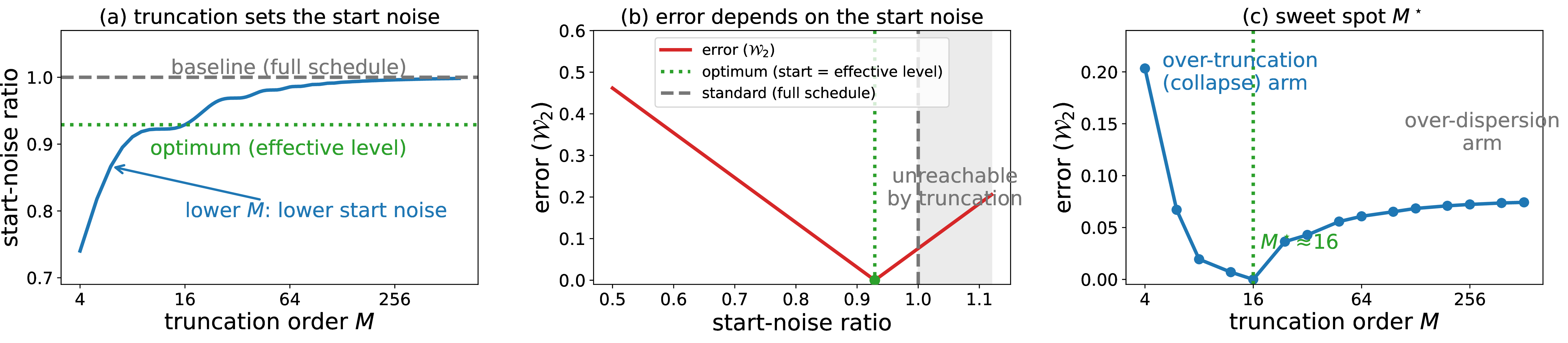
Effective noise and the sweet spot. To turn the mismatch into a prediction, we model a pretrained denoiser as the exact minimum mean-square-error (MMSE) denoiser of the data at a reduced effective noise level \(\sigma_{\mathrm{eff}}(t)\le\sigma(t)\). This deficiency is expected a priori: fitting on finitely many samples, together with the regularization implicit in early-stopped training, shrinks the variance the network reproduces, so the noise it effectively injects is sub-nominal. Sweeping the dial \(M\) moves \(\sigma_{\!M}\) across \(\sigma_{\mathrm{eff}}\), and a closed-form \(2\)-Wasserstein analysis predicts—and our experiments confirm—a non-monotone response: as the schedule is lowered, sample quality first improves, reaches an interior optimum near the effective level, then degrades back toward the baseline (1, 1). The answer to the question above is therefore concrete and actionable: a sampler should run below the prescribed schedule, at a sweet spot set by the network’s own effective level—a training-free gain on fixed checkpoints. We call the order at this optimum the effective mode count \(M^*\), and we find the same \(M^*\) whether it is located by a sampling-side sweep on pretrained checkpoints or by a training-side sweep.
Why KL? The sweet spot is a property of the mismatch itself, so any monotonically reduced schedule family exhibits it. The KL advantage is its \(t\)-dependent contraction: \(\sigma_{\!M}(t)/\sigma(t)\) varies with \(t\) where a flat rescale cannot. On CIFAR-10 a uniform-rescaling control reproduces the sweet spot but recovers only part of the KL gain (4.4); we read this as evidence—not proof—that the shaped contraction matches the network’s effective deviation better than a constant one. Finally, the same construction supplies a KL reverse-time equation and its probability-flow counterpart, yielding KL versions of standard deterministic and learned-predictor samplers (KL-DDIM, KL-DPM-Solver) at no extra network cost, with one effective order \(M^*\) governing both training and sampling.
Contributions. (i) Theory. From an exact spectral (Parseval) representation of the VP forward SDE we define the \(M\)-truncated KL forward process, prove its uniform first-order convergence to the original process, and—modelling a pretrained denoiser at a reduced effective noise level—give a closed-form \(2\)-Wasserstein analysis (1) that establishes the non-monotone sweet spot, with finite-sample shrinkage as its a priori cause and the optimal order \(M^*\) read off empirically. (ii) \(M^*\) via sampling (training-free). The KL schedule family probes \(M^*\) on pretrained checkpoints, yielding training-free gains across datasets (CIFAR-10, CelebA, ImageNet \(64^2\), Stable Diffusion v1.4) and samplers, from formula-based solvers (DDIM, DPM-Solver(++)) to the learned-predictor solver AMED (4), and extends to inverse-problem solving with DAPS. (iii) \(M^*\) via training. A controlled study shows that the sampling-side and training-side sweeps recover the same \(M^*\); training at this matched order gives the best pipeline (\(2.8\times\) faster convergence and lower FID) and a simple descending-\(M^*\) procedure (4.2). (iv) Generality. A Lévy–Ciesielski comparison shows that finite-dimensional expansion is broadly beneficial, with the \(L^2\)-optimal KL basis clearly ahead at first order and the two bases comparable at second order.
2 Related Work↩︎
2.0.0.1 Denoising Diffusion Models
DDPM [1] showed iterative Gaussian denoising can rival GANs; Song et al. [2] unified this with score-based models via SDEs, and latent diffusion [9] and classifier-free guidance [10] scaled it to high-resolution conditional synthesis. Modified forward processes have also been explored—blurring/heat dissipation [11], arbitrary degradations [12], heavy-tailed Lévy drivers [13], and fractional Brownian drivers [14]—but these replace the driving process or the degradation itself. To our knowledge, we are the first to modify the spectral content of the standard Brownian driver by finite-dimensional KL truncation, leaving the VP process family otherwise unchanged.
2.0.0.2 Accelerated Sampling
DDIM [15] recast the reverse process as a non-Markovian chain; DPM-Solver(++) [16], [17] apply exponential integrators to the probability-flow ODE; EDM [18] tunes schedule and preconditioning; Analytic-DPM [7] gives closed-form optimal per-step variance; and distillation [19], consistency models [20], rectified flows [21], and AMED [22] cut evaluations via extra training. All operate on the standard forward process; our KL samplers add a complementary, training-free dimension—they alter the noise magnitude at fixed discretization, while these methods accelerate the discretization itself.
2.0.0.3 Score Estimation Error and Schedule Mismatch
That a trained denoiser operates at a noise level different from the prescribed one is documented as structured score error [5], [6], exposure bias / Epsilon Scaling [4], train/sampling schedule defects [3], and the optimal reverse variance of Analytic-DPM [7]. These are empirical or per-step corrections of the operating point; we instead give a closed-form account of the discrepancy and its interior optimum via a one-parameter KL schedule family \(\{\sigma_{\!M}(t)\}\) (1). Unlike schedule-optimization methods that tune the time-discretization for a correctly specified score [18], [23], [24], we fix the discretization and vary the noise magnitude \(\sigma_{\!M}(t)<\sigma(t)\) at fixed \(t\)—a distinct degree of freedom.
2.0.0.4 Karhunen–Loève Expansion in Computational Science
The KL expansion is a classical, \(L^2\)-optimal spectral decomposition of stochastic processes [8], [25], widely used in stochastic finite elements [26], uncertainty quantification, random-field generation [27], and inverse problems [28]. To our knowledge this is the first use of the KL expansion of the Brownian motion driving the forward SDE to build a finite-dimensional diffusion framework.
3 The KL-Diffusion Framework↩︎
We develop the KL-Diffusion framework in full. Section 3.1 derives the exact Parseval representation. Section 3.2 introduces the truncated KL forward process. Section 3.3 recasts mode truncation as a reduced noise schedule—the noise-level dial. Section 3.4 gives the exact Gaussian analysis whose central prediction is an effective mode count \(M^*\). Section 3.5 derives the KL reverse-time equation, Section 3.6 the KL training loss (with training mode count \(M'\)), and Section 3.7 the KL sampler family (KL-DDIM, KL-Euler, KL-DPM-Solver). This prediction is then measured empirically in the experiments: 4.2 confirms \(M^*\) from both the sampling and training axes on CIFAR-10, and 4.3 probes it across datasets, samplers, and model scales.
3.1 KL Expansion of the SDE Solution↩︎
We work on \([0,T]\) and adopt the variance-preserving (VP) forward SDE 1 , with drift \(f(t)=-\tfrac12\beta(t)\) and diffusion \(g(t)=\sqrt{\beta(t)}\), where \(\beta(t) = \beta_{\min} + (\beta_{\max} - \beta_{\min})t/T\) and \(\beta_{\max}>\beta_{\min}>0\). Its solution is \[\label{eq:SDEsoln} X_t = \alpha(t)\,X_0 + \alpha(t)\!\int_0^t h(s)\,\mathrm{d}W_s,\tag{2}\] with signal-scaling factor \(\alpha(t) = \exp\!\bigl(-\tfrac{1}{2}\!\int_0^t\!\beta(s)\,\mathrm{d}s\bigr)\), reduced diffusion coefficient \(h(s) = \sqrt{\beta(s)}/\alpha(s)\), and marginal variance \(\sigma(t)^2 = 1 - \alpha(t)^2\).
The Brownian motion on \([0,T]\) admits the KL expansion [25] with eigenfunctions \(\varphi_m(t) = \sqrt{2/T}\sin\!\bigl((m\!-\!\tfrac{1}{2}) \pi t/T\bigr)\) and eigenvalues \(\lambda_m = T^2/\bigl((m\!-\!\tfrac{1}{2})^2\pi^2\bigr)\). The derivative eigenfunctions \[\label{eq:psi} \psi_m(t) := \sqrt{\lambda_m}\,\varphi_m'(t) = \sqrt{\tfrac{2}{T}}\cos\!\Bigl(\bigl(m\!-\!\tfrac{1}{2}\bigr)\tfrac{\pi t}{T}\Bigr)\tag{3}\] form a complete orthonormal basis of \(L^2([0,T])\). By the Wiener isometry [29], defining \(Z_m := \int_0^T \psi_m(s)\,\mathrm{d}W_s\), we have \(Z_m \overset{\mathrm{iid}}{\sim} \mathcal{N}(0,1)\), and Parseval’s theorem yields the exact representation of the SDE solution 2 : \[\label{eq:exact} X_t = \alpha(t)\,X_0 + \alpha(t)\sum_{m=1}^{\infty} c_m(t)\,Z_m,\tag{4}\] where \(c_m(t) := \int_0^t h(s)\,\psi_m(s)\,\mathrm{d}s\). This is exact (not an approximation) and forms the foundation of our framework: the randomness of the SDE solution can be reorganized into independent KL modes before any truncation is introduced.
3.2 The Truncated KL Forward Process↩︎
Retaining only the first \(M\) terms in 4 defines the KL forward process: \[\label{eq:XM} \begin{align} X_t^{(M)} &:= \alpha(t)\Bigl(X_0 + \sum_{m=1}^{M} Z_m\,c_m(t)\Bigr),\\ \mathbf{z}&=(Z_1,\dots,Z_M)^{\top} \sim \mathcal{N}(\mathbf{0}, I_M). \end{align}\tag{5}\] This is the \(M\)-mode approximation of 2 or 4 , with augmented Gaussian vector \(\mathbf{z}\) and deterministic temporal coefficients \(c_m(t)\). The marginal variance satisfies \[\label{eq:sigM} \sigma_{\!M}(t)^2 := \alpha(t)^2 \sum_{m=1}^{M} c_m(t)^2 \xrightarrow{M\to\infty} \sigma(t)^2,\tag{6}\] by Parseval’s theorem.
Theorem 1 (Convergence). Assume \(h \in C^1([0,T])\). Then \(\sup_{t}\,\mathbb{E}[|X_t - X_t^{(M)}|^2] \leq C/M\), where \(C = (\max_t \alpha(t))^2 \cdot A^2 / \pi^2\) with \(A = \sqrt{2}(\|h\|_\infty + \|h'\|_\infty)\).
The verification (Appendix 6, stated with the normalization \(T{=}1\); general \(T\) follows by time rescaling) exploits the fact that \(X_t - X_t^{(M)} = \alpha(t)\sum_{m>M} c_m(t)\,Z_m\) is a Parseval tail, with \(|c_m(t)| \leq A/((m\!-\!\tfrac{1}{2})\pi)\) by integration by parts.
Remark 1 (Random-ODE form). Differentiating the truncated solution 5 gives the equivalent forward equation \[\label{eq:kl-forward-sde} \mathrm{d}X_t^{(M)} = f(t)\,X_t^{(M)}\,\mathrm{d}t + g(t)\,\mathrm{d}W_t^{(M)},\tag{7}\] where \(W_t^{(M)} := \sum_{m=1}^{M} Z_m\,\sqrt{\lambda_m}\,\varphi_m(t)\) is the truncated KL Brownian motion. This is a random ODE with augmented Gaussian initial vector \(\mathbf{z}\) and deterministic temporal coefficients \(\varphi_m(t)\). It takes 5 as the unique solution.
The convergence result shows that the truncated KL forward process recovers the VP SDE as \(M\) grows, but it does not yet explain what a finite value of \(M\) means for a discretized diffusion trajectory. We next make this relation explicit through a linear system connecting the latent KL modes to time observations.
3.3 From Mode Truncation to a Reduced Noise Schedule↩︎
The truncated marginal variance 6 , \(\sigma_{\!M}(t)^2=\alpha(t)^2\sum_{m\le M}c_m(t)^2\), is non-decreasing in \(M\) and increases to \(\sigma(t)^2\) as \(M\to\infty\) (1). Because the KL driver is white noise, truncation lowers the variance of each per-time marginal without introducing non-Gaussian or cross-time structure, and a DDIM-type sampler accesses the forward process only through this per-time marginal level. The sampler therefore cannot distinguish the order-\(M\) truncated process from the full process run with the reduced schedule \(\sigma_{\!M}(t)\):
mode truncation acts, at the sampler, as a reduced noise schedule \(\sigma_{\!M}(t)<\sigma(t)\) whose contraction \(\sigma_{\!M}(t)/\sigma(t)\) varies with \(t\).
The truncation order \(M\) is thus a dial on the sampling noise level, decoupled from the time discretization; the \(t\)-dependence of \(\sigma_{\!M}/\sigma\)—as opposed to a uniform rescaling—is what later distinguishes the KL family from a constant-scaled schedule (4.4).
3.4 Exact Gaussian Analysis and the Sampling Sweet Spot↩︎
Under an isotropic Gaussian prior the score is linear, the Bayes-optimal denoiser is a Wiener filter, and the deterministic (\(\eta\!=\!0\)) DDIM chain collapses to a product of scalars. This yields an exact account of the sampled variance and of why a truncation sweet spot exists. Throughout we order the schedule in reverse time \(1=t_S>\cdots>t_0=0\) (\(t_S\) the noise end, \(t_0\) the data end), with \(S\) the number of sampler steps.
3.4.0.1 Closed-form estimators.
Take the scalar Gaussian core \(X_0\sim\mathcal{N}(0,\gamma^2)\) (the per-coordinate prior; all results extend coordinate-wise). With \(X_t=\alpha(t)X_0+\sigma(t)\boldsymbol{\epsilon}\) (3.1), the marginal of \(X_t\) is \(\mathcal{N}(0,\rho^2(t))\) with total marginal variance \[\label{eq:varrho} \rho^2(t):=\alpha(t)^2\gamma^2+\sigma(t)^2 .\tag{8}\] The optimal (MMSE) noise predictor and clean-data estimator are the Wiener filters \[\label{eq:wiener} \boldsymbol{\epsilon}^*(x,t)=\frac{\sigma(t)}{\rho^2(t)}\,x,\quad \hat{x}_0^*(x,t)=\mathbb{E}[X_0\mid X_t\!=\!x]=\frac{\alpha(t)\gamma^2}{\rho^2(t)}\,x,\tag{9}\] both linear in \(x\), with score \(\nabla_x\log p_t(x)=-x/\rho^2(t)\). These are the standard Gaussian/MMSE score and denoiser, which we cite rather than re-derive [30]–[33].
3.4.0.2 Scalar transfer coefficient and polar form.
Let \(\sigma^\dagger(t)\) denote the noise schedule used by the sampler, in the deterministic DDIM step and to set the start point, with the forward estimators 9 unchanged. Substituting 9 into the \(\eta\!=\!0\) update \(X_s^\dagger=\alpha(s)\hat{x}_0^*(X_t^\dagger,t)+\sigma^\dagger(s)\boldsymbol{\epsilon}^*(X_t^\dagger,t)\) makes each reverse step a scalar multiplication \(X_s^\dagger=A^\dagger(t,s)\,X_t^\dagger\) (\(s<t\)), with \[\label{eq:Ats} A^\dagger(t,s)=\frac{\alpha(s)\alpha(t)\gamma^2+\sigma^\dagger(s)\,\sigma(t)}{\alpha(t)^2\gamma^2+\sigma(t)^2}.\tag{10}\] The numerator is an inner product; with the data-scale diffusion angles \[\label{eq:phi-angle} \phi(t):=\arctan\frac{\sigma(t)}{\alpha(t)\gamma},\qquad \phi^\dagger(t):=\arctan\frac{\sigma^\dagger(t)}{\alpha(t)\gamma}\;\in\Big[0,\tfrac{\pi}{2}\Big),\tag{11}\] and \(\rho^\dagger(s):=\sqrt{\alpha(s)^2\gamma^2+\sigma^\dagger(s)^2}\)—so that \(\alpha(s)\gamma=\rho^\dagger(s)\cos\phi^\dagger(s)\), \(\sigma^\dagger(s)=\rho^\dagger(s)\sin\phi^\dagger(s)\) and \(\alpha(t)\gamma=\rho(t)\cos\phi(t)\), \(\sigma(t)=\rho(t)\sin\phi(t)\)—the cosine addition formula gives \(A^\dagger(t,s)=\big(\rho^\dagger(s)/\rho(t)\big)\cos\!\big(\phi(t)-\phi^\dagger(s)\big)\). Folding the data scale \(\gamma\) into the angle generalizes the angular DDIM parameterization of Salimans and Ho [19].
3.4.0.3 Output scale of the \(S\)-step chain.
Over the \(S\) steps the scalar transfers multiply, so the chain maps its start state to \(X_{t_0}^\dagger=\bigl(\prod_{k=1}^{S}A^\dagger(t_k,t_{k-1})\bigr)X_{t_S}^\dagger\), and the object to estimate is the transfer product. We approximate it in two steps. (i) Inside each transfer coefficient we set \(\sigma^\dagger\approx\sigma\), hence \(\rho^\dagger\approx\rho\) and \(\phi^\dagger\approx\phi\); by the polar form, \[\begin{align} \label{eq:Sprod} \prod_{k=1}^{S}A^\dagger(t_k,t_{k-1}) &\approx\prod_{k=1}^{S}\frac{\rho(t_{k-1})}{\rho(t_k)} \cos\bigl(\phi(t_k)-\phi(t_{k-1})\bigr)\notag\\ &=\frac{\gamma}{\rho(t_S)}\prod_{k=1}^{S}\cos\bigl(\phi(t_k)-\phi(t_{k-1})\bigr), \end{align}\tag{12}\] where the \(\rho\)-ratios telescope and \(\rho(t_0)=\sqrt{\alpha(0)^2\gamma^2+\sigma(0)^2}=\gamma\). (ii) The remaining cosine product depends on the grid only through the angle increments, which are nonnegative and sum to the total sweep \(\Phi=\phi(t_S)-\phi(t_0)=\phi(t_S)\). We replace it by its best case over grids, the discretization factor \[\label{eq:kappa} \kappa_S:=\sup\Big\{\prod_{k=1}^{S}\cos\delta_k\;:\;\delta_k\ge0,\;\sum_{k=1}^{S}\delta_k=\Phi\Big\}\;\in(0,1),\tag{13}\] attained at equal angles, \(\kappa_S=\cos^S(\Phi/S)\approx e^{-\Phi^2/2S}\) (Appendix 7); the product for any actual grid is smaller by an \(O(1/S)\) factor, an uncertainty inherited by all downstream uses of \(\kappa_S\). Thus \(\prod_{k=1}^{S}A^\dagger(t_k,t_{k-1})\approx\gamma\kappa_S/\rho(t_S)\). (iii) Finally, the chain is linear and is initialised by the sampling schedule at \(X_{t_S}^\dagger\sim\mathcal{N}\bigl(0,(\sigma^\dagger(t_S))^2 I_d\bigr)\), so the output is a centred Gaussian whose scale is approximated by \[\label{eq:eff-gamma} \sigma^\dagger(t_S)\prod_{k=1}^{S}A^\dagger(t_k,t_{k-1}) \;\approx\;\frac{\gamma\,\kappa_S}{\rho(t_S)}\,\sigma^\dagger(t_S) \;=:\;\tilde{\gamma}_S^\dagger,\tag{14}\] i.e.the output is approximately \(\mathcal{N}(0,(\tilde{\gamma}_S^\dagger)^2)\); \(\tilde{\gamma}_S^\dagger\) names the approximant on the right of 14 , not the exact output scale. After steps (i)–(ii) the sampling schedule enters the output only through its start value \(\sigma^\dagger(t_S)\).
3.4.0.4 Effective forward noise.
A finite-capacity network does not realize the prescribed forward noise exactly; within the KL family this under-realization is indexed by a finite order, i.e.a reduced schedule \(\sigma_{\!M}(t)\) (indeed, 3.6 shows that KL training at order \(M'\) is exactly training at the reduced schedule \(\sigma_{M'}\)). We therefore posit, as a modeling assumption corroborated by the experiments, an effective forward level \(\sigma_{\mathrm{eff}}(t)\le\sigma(t)\) that is deficient at the start, \(\sigma_{\mathrm{eff}}(t_S)<\sigma(t_S)\). This is the level the estimators 9 effectively use, so the prefactor \(\gamma/\rho(t_S)\) in 14 is read at it, \(\rho(t_S)\!\to\!\rho_{\mathrm{eff}}(t_S)\approx\sigma_{\mathrm{eff}}(t_S)\), while the start value \(\sigma^\dagger(t_S)\) set by the sampling schedule is untouched: \[\label{eq:tilde-corr} \tilde{\gamma}_S^\dagger\approx\gamma\,\kappa_S\,\frac{\sigma^\dagger(t_S)}{\sigma_{\mathrm{eff}}(t_S)} .\tag{15}\] The two levels now play distinct roles: \(\sigma^\dagger(t_S)\) (numerator) is the inference noise the sampler may choose, whereas \(\sigma_{\mathrm{eff}}(t_S)\) (denominator) is what the network implements; the truncated KL schedule makes \(\sigma_{\mathrm{eff}}(t_S)\) concrete through the order \(M\).
Deficiency is expected a priori from finite-sample fitting and the regularization implicit in early-stopped training (1); the same prescribed-versus-effective discrepancy is reported empirically as exposure bias / noise-level correction (2).
Definition 1 (Effective noise level). A denoiser \(\hat{x}_0^\theta(\cdot,t)\) has effective noise level \(\sigma_{\mathrm{eff}}(t)\le\sigma(t)\) if it equals the exact MMSE denoiser of the data at additive level \(\sigma_{\mathrm{eff}}(t)\), \(\hat{x}_0^\theta(x,t)=\mathbb{E}[X_0\mid \alpha(t)X_0+\sigma_{\mathrm{eff}}(t)\,\xi=x]\), \(\xi\sim\mathcal{N}(0,I)\); it is deficient when \(\sigma_{\mathrm{eff}}(t)<\sigma(t)\).
Measuring fidelity with the \(2\)-Wasserstein distance between centred isotropic Gaussians, \(\mathcal{W}_2(\mathcal{N}(0,a^2I_d),\mathcal{N}(0,b^2I_d))=\sqrt d\,|a-b|\)—a deliberate, network-free surrogate for FID that captures exactly the second-moment fidelity the Gaussian model controls—yields the sweet spot.
Proposition 1 (Sampling sweet spot). With \(D:=\mathcal{W}_2\big(\mathcal{N}(0,(\tilde{\gamma}_S^\dagger)^2 I_d),\mathcal{N}(0,\gamma^2 I_d)\big)\), \[\label{eq:parabola} \begin{align} D^2 &= d\,\gamma^2\Big(\kappa_S\,\frac{\sigma^\dagger(t_S)}{\sigma_{\mathrm{eff}}(t_S)}-1\Big)^2,\\ \text{optimum:}\quad \sigma^\dagger(t_S) &= \frac{\sigma_{\mathrm{eff}}(t_S)}{\kappa_S} . \end{align}\qquad{(1)}\] Since \(D\) is the modulus of an affine function of \(\sigma^\dagger(t_S)\), this zero is its unique global minimum. The optimal start noise sits a factor \(1/\kappa_S>1\) above the effective level: it amplifies* (\(\sigma^\dagger(t_S)>\sigma(t_S)\)) when \(\sigma_{\mathrm{eff}}(t_S)>\kappa_S\sigma(t_S)\) and attenuates (\(\sigma^\dagger(t_S)<\sigma(t_S)\)) otherwise—one formula, both regimes.*
Because \(\sigma_{\mathrm{eff}}(t_S)<\sigma(t_S)\) is assumed from the start, both regimes arise without any contradiction-then-fix; the image experiments fall in the attenuating branch (sampling below the prescribed schedule improves fidelity). The polar/tangent device coincides with that used to optimize schedules for a correctly specified score [23]; here the discretization is fixed. 1 thus establishes that the sweet spot exists, is unique, and is locatable by a one-dimensional sweep; through the \(\kappa_S\) reduction it is deliberately blind to the numerical value of \(M^*\) and to which reduced family is best—both are read from experiments. Note that if \(\sigma_{\mathrm{eff}}=\sigma\) the optimum \(\sigma(t_S)/\kappa_S\) would lie above the prescribed schedule and every reduced schedule would only degrade quality, contrary to 4: the deficiency \(\sigma_{\mathrm{eff}}<\sigma\) is the minimal modification consistent with the data. Note also that \(\sigma_{\mathrm{eff}}\) replaces the estimator-side level in 9 , not the sampler-side \(\sigma^\dagger\), so within the model it is a checkpoint property.
3.4.0.5 Realization by the KL schedule.
A physically motivated choice of the sampling schedule is the KL schedule, \(\sigma^\dagger=\sigma_{\!M}\) (3.2), realized in practice by KL-DDIM (3.7). Only the start value enters, so \[\label{eq:D-M} D(M)=\gamma\sqrt d\,\Big|\kappa_S\,\frac{\sigma_{\!M}(t_S)}{\sigma_{\mathrm{eff}}(t_S)}-1\Big| ,\tag{16}\] and as \(M\) increases \(\sigma_{\!M}(t_S)\uparrow\sigma(t_S)\), so \(\sigma_{\!M}(t_S)\) sweeps upward and crosses \(\sigma_{\mathrm{eff}}(t_S)/\kappa_S\) at an interior order \(M^*\): \(D(M)\) first falls to zero there and then rises—a single-minimum U-shape. The order at the optimum is the network’s effective mode count \(M^*\), located per checkpoint–sampler configuration; the sampling-side and training-side probes cohere at the fixed point \(M^*\!=\!M'\) (4.2). As FID is itself a Bures \(\mathcal{W}_2^2\) between Gaussian feature fits, the structural predictions—steep collapse arm, interior optimum, gentle approach to the baseline—transfer to the FID curve, though absolute values are not.
3.4.0.6 Beyond the \(\kappa_S\) reduction.
1 treats \(\sigma^\dagger\) as unknown, and \(\kappa_S\) is the price: the U-shape it delivers is governed by the start values \(\sigma(t_S)\) and \(\sigma^\dagger(t_S)\) alone, not by the profiles \(\sigma(t)\) and \(\sigma^\dagger(t)\). Once a family \(\{\sigma^\dagger_M\}\) is fixed, one mild assumption on it removes \(\kappa_S\); \(\sigma_{\mathrm{eff}}\) remains unknown but fixed. Keeping the estimators 9 at the effective level (1), the \(\eta\!=\!0\) update is again a scalar multiplication, now with \[\label{eq:Ats-exact} A^\dagger(t,s)=\frac{\alpha(s)\alpha(t)\gamma^{2}+\sigma^\dagger(s)\,\sigma_{\mathrm{eff}}(t)}{\alpha(t)^{2}\gamma^{2}+\sigma_{\mathrm{eff}}(t)^{2}} ,\tag{17}\] so a chain started at scale \(s_0\) has output scale and error \[\label{eq:Pm} s(M)=s_0\prod_{k=1}^{S}A^\dagger(t_k,t_{k-1}),\qquad D(M)=\sqrt d\,\bigl|s(M)-\gamma\bigr| .\tag{18}\]
Proposition 2 (Sweet spot without the \(\kappa_S\) reduction). Fix \(\sigma_{\mathrm{eff}}\) on the sampler grid, with \(\sigma_{\mathrm{eff}}(t_k)>0\) for some \(k\ge1\). If \(\sigma^\dagger_M(t_k)\le\sigma^\dagger_{M'}(t_k)\) at every grid point whenever \(M<M'\), with strict inequality at one of them, then \(s(M)\) is strictly increasing in \(M\). Hence \(D(M)\) falls, then rises: it has a unique minimizer, interior whenever \(s(M)\) crosses \(\gamma\) on the swept range.
Indeed, each \(A^\dagger(t_k,t_{k-1})>0\) and depends on \(M\) only through \(\sigma^\dagger_M(t_{k-1})\) in its numerator, and \(D\) is the modulus of an affine function of \(s(M)\). Since \(s_0\) does not depend on \(M\), the start convention is immaterial to the shape: our samplers initialize from \(X_{t_S}\sim\mathcal{N}(0,I_d)\), as standard DDIM does. The KL, \(\nu\)- and Lévy–Ciesielski families all meet the hypotheses of both propositions, so each exhibits the U-shape; this is the statement the experiments of [sec:train-scratch,sec:pretrained-samplers,sec:rho] test. The KL reverse-time equation, training loss, and samplers are developed next.
3.5 KL Reverse-Time Equation↩︎
Since the truncated KL forward process is a random ODE rather than an Itô SDE, we construct its reverse-time counterpart indirectly: we first introduce an auxiliary Itô SDE whose marginals match those of the KL forward process in the \(M\to\infty\) limit (exact matching is generally impossible at finite \(M\); Supplementary App. H), apply Anderson’s reversal to that SDE, and then truncate the reverse noise in the KL basis. The result is a principled approximate reversal, exact as \(M\to\infty\); among our samplers only KL-Euler depends on it, while KL-DDIM and KL-DPM-Solver are defined directly from the exact per-time marginals of 5 (Supplementary App. H). Given terminal state \(X_T^{(M)}\) and fresh expansion coefficients \(\{\bar{Z}_m\}_{m=1}^M \overset{\mathrm{iid}}{\sim} \mathcal{N}(0,1)\), the KL reverse-time equation is: \[\begin{align} \frac{\mathrm{d}X_t}{\mathrm{d}t} &= f(t)\,X_t - g_{\!M}^2(t)\,\nabla_X \log p_t^{(M)}(X_t) \nonumber\\ &\quad + g_{\!M}(t)\sum_{m=1}^{M} \psi_m(t)\,\bar{Z}_m . \label{eq:kl-reverse} \end{align}\tag{19}\] where \(\nabla_X \log p_t^{(M)}(X_t)\) is the score function for the KL forward equation 7 , \(g_{\!M}(t) = \sqrt{\beta(t)}\,\sigma_{\!M}(t)/\sigma(t)\) is the effective diffusion coefficient of the truncated process, and \(\psi_m(t)\) are the cosine basis functions from 3 . The fresh coefficients \(\{\bar{Z}_m\}_{m=1}^{M} \overset{\mathrm{iid}}{\sim} \mathcal{N}(0,1)\) are drawn once and held fixed for the entire reverse trajectory. Once drawn, the third term—the expansion force—becomes a known smooth function of \(t\), reducing 19 to a deterministic ODE amenable to standard high-order solvers. The \(\{\bar{Z}_m\}\) are independent of the forward \(\{Z_m\}\); Anderson’s time-reversal theorem [34] and the Fokker–Planck constraint require only equality in distribution, not sample-level correspondence.
Remark 2 (Connection to samplers). Existing samplers discretize the continuous reverse SDE. By starting from the KL reverse-time equation 19 instead, we obtain a family of KL samplers whose coefficients naturally involve \(\sigma_{\!M}(t)\) rather than \(\sigma(t)\).
3.6 KL Training Loss↩︎
The KL forward process 5 directly induces a training loss. Write \(M'\) for the training truncation order (the training mode count; standard training is \(M'\!=\!\infty\)) and \(M\) for the sampler order. Drawing \(X_0\sim p_{\mathrm{data}}\), \(\mathbf{z}\sim\mathcal{N}(0,I_{M'})\), and \(t\), the noised sample is \(X_t^{(M')}=\alpha(t)X_0+\sigma_{M'}\!(t)\hat{\boldsymbol{\epsilon}}\) with \(\hat{\boldsymbol{\epsilon}}=\alpha(t)\sum_{m=1}^{M'}Z_m c_m(t)/\sigma_{M'}\!(t)\); by additivity of independent Gaussians \(\hat{\boldsymbol{\epsilon}}\sim\mathcal{N}(0,1)\) exactly, so for a single-time marginal the KL loss \[\label{eq:kl-loss} \mathcal{L}_{\mathrm{KL}}=\mathbb{E}_{t,X_0,\mathbf{z}}\big[\|\boldsymbol{\epsilon}_\theta(X_t^{(M')},t)-\hat{\boldsymbol{\epsilon}}\|^2\big]\tag{20}\] is implemented by drawing \(\boldsymbol{\epsilon}\sim\mathcal{N}(0,I)\) and scaling by \(\sigma_{M'}\!(t)\); it differs from the standard loss only in the reduced noise level and recovers it as \(M'\!\to\!\infty\). We adopt this single-time loss and leave multi-time KL objectives to future work.
3.7 KL Samplers↩︎
The KL reverse-time equation 19 provides a principled starting point for deriving samplers of increasing sophistication. Throughout the experiments, \(S\) denotes the number of sampler steps. We present the canonical KL-DDIM sampler first—the workhorse of our experiments—followed by KL-Euler and the higher-order KL-DPM-Solver variants.
3.7.1 KL-DDIM\((M, \eta)\)↩︎
KL-DDIM is the canonical KL sampler used throughout our experiments: it is the popular deterministic DDIM solver, the order-1 base case to which the higher-order KL solvers reduce, and its clean \((M,\eta)\) knobs make it the natural vehicle for both the \(S\)-sweep and the \(M\)-sweep. KL-DDIM is derived from the KL probability flow ODE—the deterministic counterpart of 19 obtained by dropping the expansion force and halving the score coefficient: \[\dot{X}_t = f(t)\,X_t - \tfrac{1}{2}g_{\!M}^2(t)\,\nabla_X \log p_t^{(M)}(X_t).\] The resulting update is identical to standard DDIM [15] with the replacement \(\sigma(\cdot) \to \sigma_{\!M}(\cdot)\) in both the predicted \(\hat{X}_0\) and the directional step: \[\begin{align} \label{eq:kl-ddim} \hat{X}_0 &= \bigl(X_s - \sigma_{\!M}(s)\,\boldsymbol{\epsilon}_\theta(X_s,s)\bigr) / \sqrt{\bar\alpha_s}, \notag\\ X_t &= \sqrt{\bar\alpha_t}\,\hat{X}_0 + \sqrt{\sigma_{\!M}^2(t) - \tilde{\sigma}_\eta^2}\;\boldsymbol{\epsilon}_\theta(X_s,s) + \tilde{\sigma}_\eta\,\boldsymbol{\epsilon}, \end{align}\tag{21}\] where \(\tilde{\sigma}_\eta^2 = \eta^2\,\sigma_{\!M}^2(t)\, \bigl(1 - \bar\alpha_s\,\sigma_{\!M}^2(t)/(\bar\alpha_t\,\sigma_{\!M}^2(s))\bigr)\), with \(\bar\alpha_t = \alpha(t)^2\) as before. At \(\eta = 0\), the sampler is purely deterministic, and \(\sigma_{\!M}(t) < \sigma(t)\) reduces the directional coefficient, yielding a less aggressive correction at each step. Because KL-DDIM is derived from the KL probability flow ODE—whose coefficients involve \(\sigma_{\!M}(t)\) through the marginal variance of the KL forward process—the schedule \(\sigma_{\!M}(t)\) enters the sampler as a consequence of the derivation, not as a heuristic substitution. The resulting implementation differs from standard DDIM only in replacing \(\sigma(t)\) with the precomputed \(\sigma_{\!M}(t)\). Equivalently, and without reference to the reverse-time equation, KL-DDIM is exactly the non-Markovian DDIM construction of [15] applied to the per-time marginals \(\mathcal{N}\bigl(\alpha(t)X_0,\sigma_{\!M}^2(t)I\bigr)\) of the KL forward process, which 5 supplies in closed form. All KL samplers initialize from \(X_{t_S}\sim\mathcal{N}(0,I)\), as standard DDIM does; by 2 the start convention does not affect the shape of the \(M\)-response. For \(\eta > 0\), the same KL-DDIM formula injects fresh i.i.d. noise \(\boldsymbol{\epsilon}\sim \mathcal{N}(0,I)\) scaled by \(\tilde{\sigma}_\eta\), exactly as in the stochastic branch of standard DDIM; no separate sampler is introduced for this case.
3.7.2 KL-Euler\((M)\)↩︎
The most direct approach is to apply the Euler method to the KL reverse-time equation 19 . Given a discretization \(1 = t_S > t_{S-1} > \cdots > t_0 = 0\) with step sizes \(\Delta t_k = t_k - t_{k-1}\), the update is: \[\begin{align} X_{t_{k-1}} &= X_{t_k} - \Delta t_k\!\Bigl[ f(t_k)\,X_{t_k} \nonumber\\ & + \frac{g_{\!M}^2(t_k)}{\sigma_{\!M}(t_k)}\,\boldsymbol{\epsilon}_\theta(X_{t_k}, t_k) + g_{\!M}(t_k)\sum_{m=1}^{M} \psi_m(t_k)\,\bar{Z}_m \Bigr],\label{eq:kl-euler} \end{align}\tag{22}\] where we approximate the score via the \(\boldsymbol{\epsilon}\)-parameterization: \(\nabla_X \log p_t^{(M)}(X_t) \approx -\boldsymbol{\epsilon}_\theta(X_t, t)/\sigma_{\!M}(t)\) (here \(\boldsymbol{\epsilon}_\theta\) is trained at the prescribed level unless the KL loss of 3.6 is used; this gap is the mismatch analyzed in 3.4). The expansion coefficients \(\{\bar{Z}_m\}\) are drawn once and reused at every step, providing a structured noise trajectory that contrasts with the i.i.d.noise in the standard reverse SDE Euler. KL-Euler uses all \(S=1000\) time steps (the original DDPM schedule) and serves as the baseline for the KL sampler family.
3.7.3 KL-DPM-Solver\((M, k)\)↩︎
The KL probability flow ODE admits the variation-of-constants (VoC) formulation used by DPM-Solver [16]. Substituting \(X_t = \alpha(t)\,u_t\) converts the ODE to \(\dot{u}_t = -\tfrac{1}{2}g_{\!M}^2(t)\,\boldsymbol{\epsilon}_\theta / (\alpha(t)\,\sigma_{\!M}(t))\). Integration from \(s\) to \(t\) gives \[\label{eq:kl-dpm-update} X_t = \frac{\alpha(t)}{\alpha(s)}\,X_s + \alpha(t)\!\int_{\lambda_{\!M}(s)}^{\lambda_{\!M}(t)}\! e^{-\lambda}\,\hat{\boldsymbol{\epsilon}}_\theta\;\mathrm{d}\lambda,\tag{23}\] where \(\lambda_{\!M}(t) := \log\bigl(\sqrt{\bar\alpha_t}/\sigma_{\!M}(t)\bigr)\) is the KL log-SNR. The integral is approximated by Taylor expansion of \(\hat{\boldsymbol{\epsilon}}_\theta\) in \(\lambda\).
Order 1. Freezing \(\hat{\boldsymbol{\epsilon}}_\theta\) at \(\lambda_s\) yields the first-order update, equivalent to KL-DDIM at \(\eta=0\).
Order 2 (multistep). Using two consecutive model evaluations \(\hat{\boldsymbol{\epsilon}}_s\), \(\hat{\boldsymbol{\epsilon}}_{s'}\) (with \(s' < s\)), the corrected prediction is \[\hat{\boldsymbol{\epsilon}}_{\mathrm{corr}} = \hat{\boldsymbol{\epsilon}}_s + \frac{1}{2r}\bigl(\hat{\boldsymbol{\epsilon}}_s - \hat{\boldsymbol{\epsilon}}_{s'}\bigr), \quad r = \frac{\lambda_{\!M}(s) - \lambda_{\!M}(s')}{\lambda_{\!M}(t) - \lambda_{\!M}(s)}.\] The first-order update 23 is then applied with \(\hat{\boldsymbol{\epsilon}}_{\mathrm{corr}}\). A key implementation detail is that the log-SNR schedule \(\lambda_{\!M}(t)\) differs from \(\lambda(t)\), affecting the extrapolation ratio \(r\). The ratio \(\sigma_{\!M}(t)/\alpha(t)=\bigl(\sum_{m\le M}c_m(t)^2\bigr)^{1/2}\) is strictly increasing in \(t\) (verified numerically on our schedule for all \(M\in[2,1024]\)), so \(\lambda_{\!M}\) is strictly monotone and \(r\) is well-defined at every \(M\); \(\sigma_{\!M}(t)\) itself is non-monotone in the high-noise region but never enters the solver through a ratio. In our experiments, order-2 with \(M\!=\!256\) gives the best KL-DPM result.
3.7.3.1 KL-DPM-Solver++ and other samplers
DPM-Solver++ [17] expands the data prediction \(\hat{x}_0(\lambda)\) (order 2 is the standard guided sampler for Stable Diffusion). KL truncation enters only through the data prediction, \(\hat{x}_{0,\mathrm{KL}}=(x-\sigma_{\!M}\hat{\boldsymbol{\epsilon}})/\alpha\), leaving all ODE transition coefficients at the standard \(\sigma\) and preserving order-2 stability; on SD v1.4 KL-DPM++ (\(M\!=\!64\)) improves over DPM-Solver++ and LoRA-KL-DPM++ (\(M\!=\!32\)) is best (6). More generally the \(\sigma\to\sigma_{\!M}\) substitution extends to any schedule-dependent sampler: for the learned predictor AMED [22], KL-AMED replaces only the step-size terms \((\sigma_{\mathrm{next}}-\sigma_{\mathrm{cur}})\to(\sigma_{\!M}(\sigma_{\mathrm{next}})-\sigma_{\!M}(\sigma_{\mathrm{cur}}))\), with predictor outputs and denoiser conditioning unchanged (Supplementary App. F).
4 Experiments↩︎
4.1 Setup↩︎
4.1.0.1 Datasets.
CIFAR-10 (\(32\!\times\!32\), 50k training images), CelebA [35] (\(64\!\times\!64\), 202k images), ImageNet [36] (\(64\!\times\!64\), 1.28M training images, 1000 classes), and Stable Diffusion v1.4 [9] (COCO val2014, 512\(\times\)512).
4.1.0.2 Models and checkpoint abbreviations
For CIFAR-10, we use two checkpoints: PFDiff-790k, the PFDiff EMA pretrained checkpoint [37] used for sampler and LoRA comparisons, and Scratch-2040, the UNet trained from scratch for 2040 epochs to evaluate the KL training loss. For CelebA, CelebA-DDIM denotes the pretrained DDIM checkpoint from [15]. For ImageNet, EDM-ImageNet64 denotes the pretrained EDM checkpoint [18] with the VE-SDE parameterization (\(\sigma_{\min}\!=\!0.002\), \(\sigma_{\max}\!=\!80\), polynomial schedule \(\rho\!=\!7\)). The AMED-predictor [22] is a lightweight network trained on top of EDM-ImageNet64 to predict per-step adaptive parameters (4 steps with AFS, NFE\(\!=\!5\)). For Stable Diffusion, SD-v1.4 denotes the public Stable Diffusion v1.4 checkpoint with classifier-free guidance (\(w\!=\!7.5\)). For orientation across checkpoints: KL-DDIM (\(M{=}128\), \(S{=}20\), \(\eta{=}0\)) attains FID-50k \(5.07\) on PFDiff-790k, \(4.77\) on the epoch-1080 scratch checkpoint, and \(4.98\) on Scratch-2040; throughout, every quoted FID names its checkpoint.
4.1.0.3 Evaluation
FID [38] computed with 50k generated samples (FID-50k) for main results and 5k samples for ablations. All experiments use quadratic timestep scheduling; all samplers, baselines included, share this grid, so every comparison isolates the noise magnitude at fixed discretization. Generation uses 4 GPUs with per-GPU seed offsets, and our conclusions rest on the shape of entire \(M\)- and \(S\)-sweeps rather than on isolated pairwise differences. Code, configurations, and evaluation scripts will be released upon publication.
4.2 Train-from-Scratch: Locating the Effective Mode Count \(M^*\)↩︎
The train-from-scratch setting is the controlled experiment for the prediction of 3.4: unlike a fixed pretrained checkpoint, here we can set the training order \(M'\) and watch the network’s own sweet spot \(M^*\) respond. We answer the two questions posed in 3.4 on CIFAR-10 (Scratch-2040; protocol in 4), and show that the sampling-side and training-side sweeps are two views of the same effective mode count \(M^*\).
4.2.0.1 Sampling axis: \(M^*\) on a standard checkpoint.
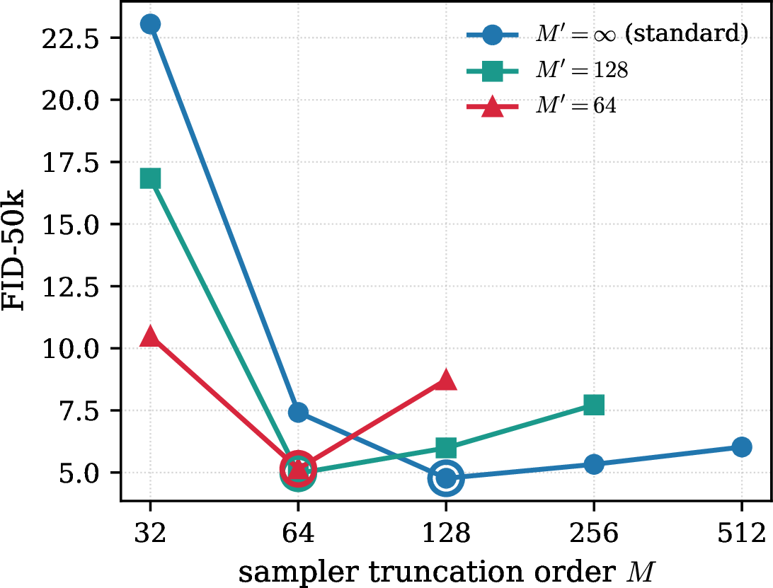
Take the standard train-from-scratch checkpoint (\(M'\!=\!\infty\), epoch 1080) and, without any retraining, sweep the KL-DDIM order \(M\) (\(\eta\!=\!0\), \(S\!=\!20\)). The FID curve is strongly non-monotone (3): it falls from \(23.03\) at \(M\!=\!32\) to a minimum of \(4.77\) at \(M\!=\!128\), then rises monotonically (\(5.29\) at \(M\!=\!256\), \(6.00\) at \(M\!=\!512\)) as \(\sigma_{\!M}\!\to\!\sigma\). The standard DDIM sampler (the \(M\!=\!\infty\) limit) gives \(6.63\) on this checkpoint, so the sweet spot at \(M^*\!=\!128\) is a \(28\%\) training-free improvement. A network trained to resolve the infinite-mode driver thus behaves, at sampling time, as if its effective mode count were finite, matching the effective-noise prediction of 1.
4.2.0.2 Training axis: matched KL training.
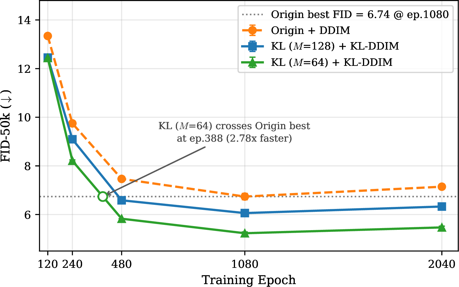
Training instead under the KL forward process at a finite order \(M'\) and evaluating with the matched KL-DDIM (\(M\!=\!M'\)) improves the diagonal \(M\!=\!M'\) result monotonically as \(M'\) decreases toward \(M^*\) (1, 2). KL(\(M'\!=\!64\))+KL-DDIM reaches FID = 5.47 at epoch 2040 versus 7.14 for Origin+DDIM, while KL(\(M'\!=\!128\)) reaches 6.33. KL(\(M'\!=\!64\)) surpasses the best Origin+DDIM checkpoint at any epoch (FID = 6.74, epoch 1080) already at epoch 480 (FID = 5.83), with \(2.25\times\) fewer epochs; linear interpolation between epochs 240 and 480 places the crossing at epoch \(\approx 388\), a \(\approx2.8\times\) training-convergence speedup under matched 20-step evaluation (highlighted line in 2). Best checkpoint against best checkpoint, the comparison is 6.74 vs.. Each entry of 1 is a mean over three sampling seeds; the spread is small (\(\le\!0.13\) FID on the noisiest row), and we report it here as a representative example rather than for every table.
4.2.0.3 The two axes meet: a descending-\(M^*\) procedure.
The sampling-side and training-side views coincide. Per-checkpoint \(M\)-sweeps (3) show that the sweet spot \(M^*\) of a KL-trained network sits at or below its training order \(M'\), and that each retraining at \(M'\!=\!M^*\) shifts the whole curve down and to the left:
\(M'\!=\!\infty\) (standard): \(M\)-sweep minimum at \(M^*\!=\!128\);
\(M'\!=\!128\): minimum moves to \(M^*\!=\!64\) (\(M\!=\!64\) beats \(M\!=\!128\), \(4.97\) vs \(5.99\)), i.e.the network still cannot use all \(128\) trained modes;
\(M'\!=\!64\): minimum is at \(M^*\!=\!64\!=\!M'\) (\(M\!=\!64\) beats both \(M\!=\!32\) and \(M\!=\!128\)), so the gap \(|M^*\!-\!M'|\) has closed and the procedure terminates.
This yields a simple recipe: train at \(M'\), locate \(M^*\) by a sampling-side \(M\)-sweep, retrain at \(M'\!\leftarrow\!M^*\), and repeat until \(M^*\!=\!M'\). The FID gain from the search itself is modest; its value is mechanistic—it exhibits a checkpoint at the fixed point \(M^*\!=\!M'\), confirming \(M^*\) as a real, controllable property recovered by either probe. We present it as an empirical heuristic: it terminates in two iterations here, but we do not establish general convergence.
4.2.0.4 Interpretation.
The KL loss differs from the standard loss only in the reduced level \(\sigma_{M'}(t)\) and recovers it as \(M'\!\to\!\infty\) (3.6), so the framework extends to training. The descending procedure terminates where the sampling-side sweep confirms the network realizes the level it was trained at; this also explains why \(M'\!=\!64\) beats \(M'\!=\!128\) even though the latter is the closer approximation to the full SDE by 1—the \(M'\!=\!128\) checkpoint’s own sweet spot sits at \(M^*\!=\!64\). Faster convergence at reduced training levels is consistent with known effects of the training noise-level distribution [6] and is not by itself evidence for the mechanism; the identifying evidence is the sweep structure, an inference-time measurement. The study is a matched-budget comparison (shared architecture, optimizer, and epochs), so its absolute FIDs are not comparable to the separately trained PFDiff-790k.
Having established \(M^*\) as a real, controllable property of the trained network, we next show that the same \(M^*\) can be read off fixed pretrained checkpoints, where it yields training-free gains across datasets, samplers, and scales (4.3).
| Epoch | Origin + DDIM | KL(\(M'\)=128) | KL(\(M'\)=64) |
|---|---|---|---|
| 120 | \(13.34\pm0.08\) | \(12.45\pm0.08\) | \(12.44\pm0.08\) |
| 240 | \(9.75\pm0.07\) | \(9.09\pm0.06\) | \(\best{8.21}\pm0.04\) |
| 480 | \(7.47\pm0.07\) | \(6.58\pm0.05\) | \(\best{5.83}\pm0.01\) |
| 1080 | \(6.74\pm0.13\) | \(6.06\pm0.09\) | \(\best{5.23}\pm0.05\) |
| 2040 | \(7.14\pm0.10\) | \(6.33\pm0.08\) | \(\best{5.47}\pm0.05\) |
4pt
4.3 Pretrained Model: KL Samplers↩︎
Using PFDiff-790k (no retraining), we evaluate KL samplers against standard baselines.
4.3.0.1 KL-Euler
As the simplest KL sampler, KL-Euler uses all \(S\!=\!1000\) DDPM steps. At \(M\!=\!128\) it achieves FID = 7.83 (FID-5k), within 0.06 of DDPM (7.77) and clearly ahead of DDIM-100 (8.91; all FID-5k), showing that the structured KL noise trajectory costs essentially nothing even for the basic 1000-step solver (full \(M\)-sweep in Supplementary App. D).
4.3.0.2 KL-DDIM
KL-DDIM (\(M\!=\!128\)) is the best deterministic sampler at every step count (2), cutting FID by 27% at \(S\!=\!20\) (\(6.90\!\to\!5.07\)) and staying ahead through \(S\!=\!100\) (\(4.19\!\to\!3.64\)).
4.3.0.3 KL-DPM-Solver
KL-DPM O2 (\(M\!=\!256\)) improves on DPM-Solver O2 at every step count (2), e.g.FID = 4.11 vs. at \(S\!=\!20\) (an 11% improvement). At very aggressive step counts the substitution breaks down (\(S\!=\!4\): 72.1 vs., Supplementary App. E), delimiting the few-step validity of the KL schedule in high-order solvers.
4.3.0.4 Cross-sampler analysis
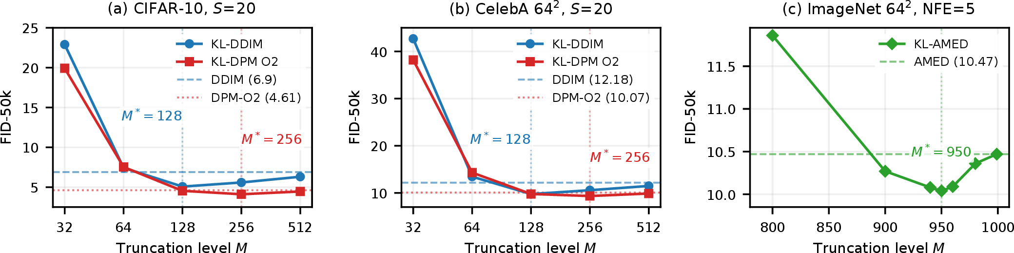
Two patterns emerge across the KL samplers. First, the benefit grows with solver order (Euler \(\to\) DDIM \(\to\) DPM O2): KL-Euler only matches its baseline (7.83 vs. FID-5k, a 0.8% regression), while KL-DDIM improves 27% over DDIM at \(S\!=\!20\) and KL-DPM O2 improves 11% over DPM-Solver O2. This extends further to learned-predictor samplers (4.5). Second, the optimal \(M\) increases with solver quality: \(M\!=\!128\) for DDIM, \(M\!=\!256\) for DPM O2, and \(M\!=\!950\) for AMED on ImageNet (4). Measured at the start level, this variation is small: \(\sigma_{\!M}(t_S)/\sigma(t_S)\approx0.994\) at \(M\!=\!128\) versus \(\approx0.997\) at \(M\!=\!256\), a sub-percent difference. Because \(\sigma_{\!M}(t_S)\) saturates as \(M\) grows, the integer \(M\) is a stretched coordinate that magnifies small level differences: the operating level identified by the sweeps is nearly sampler-invariant even though \(M^*\) is not; why the swept order depends on the sampler remains open (5).
4.3.0.5 Effective noise schedule of pretrained models.
KL samplers improve checkpoints never trained at the KL noise level, contrary to the usual assumption that training and sampling schedules must match [3]. The \(M\)-sweep is non-monotone across all datasets, samplers, and SDE frameworks (4): very small \(M\) underperforms (the gap \(|\sigma-\sigma_{\!M}|\) too large), large \(M\) approaches the baseline as \(\sigma_{\!M}\!\to\!\sigma\) (e.g.KL-DDIM at \(M\!=\!512\) gives FID = 6.27 vs.), and an intermediate \(M\) is best—the steep collapse arm, interior minimum near \(\sigma_{\!M}\!\approx\!\sigma_{\mathrm{eff}}\), and gentle over-dispersion arm of [prop:sweetspot,fig:sweetspot]. A monotone mismatch would give no interior minimum; the interior optimum signals that the network’s effective noise level lies below \(\sigma(t)\), as expected a priori from finite-sample shrinkage (1). This sweet-spot order is the effective mode count \(M^*\); 4.2 shows the training-side sweep recovers the same \(M^*\).
4.3.0.6 Distinguishing ODE conditioning from schedule matching
One alternative is that \(\sigma_{\!M}<\sigma\) merely better-conditions the probability-flow ODE. Three observations disfavor it: (i) stochastic KL-DDIM (\(\eta>0\), Supplementary Table IV) gains more than the deterministic case, whereas conditioning benefits should shrink under injected noise; (ii) the gain persists at large \(S\) (2, \(S\!=\!100\)), where discretization error is negligible; and (iii) KL-DAPS (7) improves an annealing sampler that integrates no probability-flow ODE. These favor the schedule-matching interpretation.
| Sampler | \(M\) | \(S\!=\!10\) | \(S\!=\!20\) | \(S\!=\!50\) | \(S\!=\!100\) |
|---|---|---|---|---|---|
| DDIM | — | 13.51 | 6.90 | 4.69 | 4.19 |
| DPM-Solver O2 | — | 6.60 | 4.61 | 4.34 | 4.28 |
| KL-DDIM | 128 | 9.45 | 5.07 | ||
| KL-DPM O2 | 128 | 6.21 | 4.54 | 4.28 | 4.20 |
| KL-DPM O2 | 256 | 3.91 | 3.85 |
4pt
Stochastic KL-DDIM (\(\eta > 0\)) also outperforms DDIM at every matched \(\eta\), with the largest gain at \(\eta\!=\!0.5\) (\(-36\%\)); full KL-DPM \(M\)/\(S\)-sweep curves and the stochastic table appear in Supplementary App. E.
4.4 Why KL? A Uniform-Rescaling (\(\nu\)-Sampler) Control↩︎
The analysis attributes the sweet spot to the effective-noise mismatch, not to the KL basis: 2 assumes only that the family is pointwise monotone in \(M\), so it predicts the same U-shape for any monotone reduced schedule and is silent on which family reaches the lower optimum. Whether KL beats a flat rescale is therefore an empirical question. We test the simplest constant-\(\nu\) family, the \(\nu\)-sampler \(\sigma^\dagger_M(t)=\nu_M\,\sigma(t)\) with \(\nu_M=1-1/M\) (\(\nu\)-DDIM), the schedule-space analogue of the constant \(\varepsilon\)-scaling of Ning et al. [4]. On CIFAR-10 (\(S\!=\!20\), \(\eta\!=\!0\)), \(\nu\)-DDIM indeed produces the same interior optimum (3), confirming the sweet spot is a property of the mismatch, not the basis. Yet the KL optimum is better: \(4.98\) at \(M^*\!=\!128\) beats the \(\nu\)-sampler optimum (\(5.37\) at \(M^*\!\approx\!192\)–\(224\)) at a stronger modification; away from their optima the two families cross (for \(M\!\gtrsim\!224\) the \(\nu\) row is lower), so the comparison of interest is between the family optima. We attribute the remaining gain to KL’s \(t\)-dependent contraction—the interior-profile effect the analysis is silent on—as the natural interpretation; the control compares the two families’ optima and does not isolate the mechanism itself. We therefore use KL schedules throughout. This control is a single-dataset, single-sampler comparison (CIFAR-10, KL-DDIM, \(S\!=\!20\)), and since we compare the optima of the two families, it does not depend on the particular indexing \(\nu_M\!=\!1-1/M\) of constant rescalings.
| \(M\) | 64 | 128 | 160 | 192 | 224 | 256 |
|---|---|---|---|---|---|---|
| \(\nu\)-DDIM | 14.90 | 6.12 | 5.54 | 5.42 | ||
| KL-DDIM | 7.17 | 5.13 | 5.33 | 5.49 | 5.65 |
4pt
4.5 Generality: Datasets, Samplers, and Scale↩︎
4 collects \(M\)-sweep curves across three datasets and sampler families. All panels exhibit the same non-monotone pattern identified on CIFAR-10 in 4.3: FID improves as \(M\) decreases from the baseline, reaches a sweet spot, then degrades for small \(M\). The optimal \(M\) varies by configuration, but the shape is invariant. 4 summarizes the best result per configuration.
| Dataset | Sampler | \(S\) | Baseline | Best \(M\) | KL FID |
|---|---|---|---|---|---|
| CIFAR-10 | KL-DDIM | 20 | 6.90 | 128 | |
| CIFAR-10 | KL-DPM O2 | 20 | 4.61 | 256 | |
| CelebA | KL-DDIM | 20 | 12.18 | 128 | |
| CelebA | KL-DPM O2 | 20 | 10.07 | 256 | |
| ImageNet | KL-AMED | 5 | 10.47 | 950 |
4pt
4.5.0.1 CelebA \(64\!\times\!64\)
5 shows consistent improvements: KL-DDIM (\(M\!=\!128\)) reduces FID by 20% at \(S\!=\!20\) (12.18 \(\to\) 9.76) and 10% at \(S\!=\!100\) (9.71 \(\to\) 8.77). The \(M\)-sweep pattern (4b) matches CIFAR-10, with minimum near \(M\!=\!128\) for KL-DDIM and \(M\!=\!256\) for KL-DPM. The optimal orders are unchanged from CIFAR-10 despite the fourfold change in resolution and dataset.
| Sampler | \(M\) | \(S\!=\!10\) | \(S\!=\!20\) | \(S\!=\!50\) | \(S\!=\!100\) |
|---|---|---|---|---|---|
| DDIM | — | 17.46 | 12.18 | 10.17 | 9.71 |
| DPM-O2 | — | 12.67 | 10.07 | 9.65 | 9.58 |
| KL-DDIM | 128 | 13.54 | |||
| KL-DPM O2 | 256 | 9.35 | 9.12 | 9.04 |
4pt
4.5.0.2 KL-AMED on ImageNet \(64\!\times\!64\)
AMED [22] represents a fundamentally different sampler class: a trained predictor network outputs per-step adaptive parameters \((r, s_{\mathrm{dir}}, s_{\mathrm{time}})\) from denoiser encoder features, targeting aggressive NFE\(\!=\!5\). KL-AMED applies the same \(\sigma \to \sigma_{\!M}\) step-size substitution (Supplementary App. F); predictor outputs and denoiser conditioning are unchanged, and the predictor is reused frozen from the released checkpoint. The VE-grid construction of \(\sigma_{\!M}\) is a discrete analogue outside the VP setting of 1 and is justified here empirically. 4c shows the \(M\)-sweep on ImageNet \(64\!\times\!64\) (EDM, VE-SDE): the sweet spot is \(M\!=\!950\) (FID = 10.04 vs baseline 10.47, \(-4.1\%\)), with a broad flat optimum \(M \in [940, 960]\). (Baseline FIDs are from our reproduction using the released checkpoints and may differ slightly from the values in the original papers.) Despite operating in a different SDE framework (VE vs VP), on a larger class-conditional dataset (1000 classes, 1.28M images), and with a learned rather than formula-based sampler, the non-monotone sweet-spot pattern is preserved.
4.5.0.3 Stable Diffusion v1.4
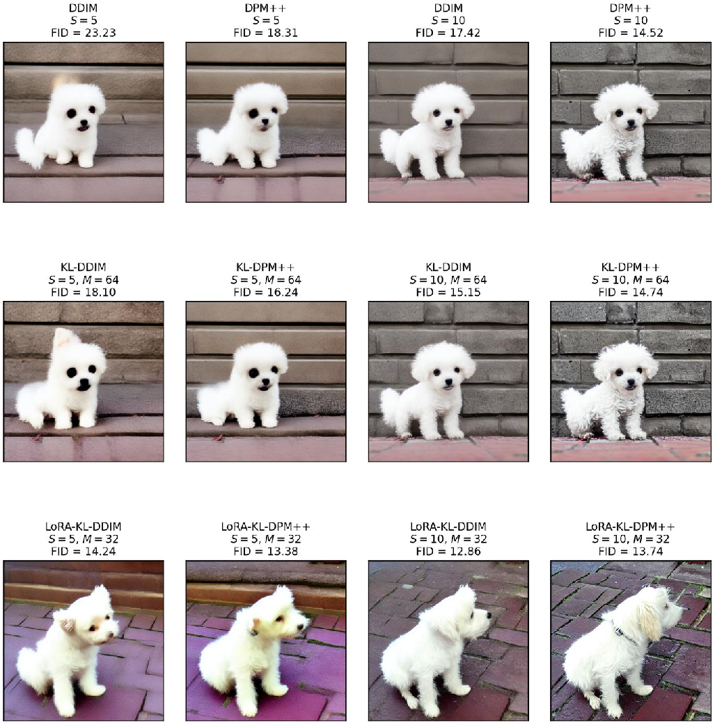
To demonstrate applicability at scale, we evaluate KL samplers on Stable Diffusion v1.4 in the \(4\!\times\!64\!\times\!64\) latent space (6). KL-DDIM (\(M\!=\!64\)) improves over DDIM at both NFE values (18.10 vs 23.23 at NFE\(\!=\!5\); 15.15 vs 17.42 at NFE\(\!=\!10\)). KL-DPM++ (\(M\!=\!64\)) improves over DPM-Solver++ at NFE\(\!=\!5\) (16.24 vs 18.31) but is slightly worse at NFE\(\!=\!10\) (14.74 vs 14.52), suggesting that the KL schedule benefit is strongest in the few-step regime where discretization error dominates. LoRA-KL-DPM++ (\(M\!=\!32\)) achieves the best NFE\(\!=\!5\) FID (13.38), while LoRA-KL-DDIM (\(M\!=\!32\)) achieves the best NFE\(\!=\!10\) FID (12.86). The lower optimal \(M\!=\!64\) (vs.\(M\!=\!128\) for CIFAR-10/CelebA) may reflect the reduced temporal complexity of latent-space diffusion.
| Sampler | \(M\) | NFE\(=5\) | NFE\(=10\) |
|---|---|---|---|
| DDIM | — | 23.23 | 17.42 |
| DPM-Solver++ [17] | — | 18.31 | 14.52 |
| KL-DDIM | 64 | 18.10 | 15.15 |
| KL-DPM++ | 64 | 16.24 | 14.74 |
| LoRA-KL-DDIM | 32 | 14.24 | |
| LoRA-KL-DPM++ | 32 | 13.74 |
4pt
4.5.0.4 Synthesis
Across six sampler–dataset combinations ([tab:kl-summary,tab:sd-fid,fig:msweep-universal]) the non-monotone sweet-spot pattern is invariant, while the optimal order varies (e.g.\(M\!=\!128\) for KL-DDIM, \(256\) for KL-DPM O2, \(950\) for KL-AMED, \(64\) for latent-space SD). Every tested checkpoint, regardless of architecture, dataset, or SDE framework, thus behaves as if internalizing a noise level slightly below \(\sigma(t)\) that the KL family \(\{\sigma_{\!M}(t)\}\) probes; the sole regression among the pairs tested in these tables is KL-DPM++ at NFE\(\,=\,\)10 on SD (6); KL-Euler is on par with DDPM, and the few-step breakdown at \(S\!=\!4\) is delimited in Supplementary App. E. In practice the sweep need not use the full protocol: on CIFAR-10, where we computed both, a cheap FID-5k sweep selects the same sweet-spot order as FID-50k (KL-DDIM \(M\!=\!128\); KL-DPM O2 \(M\!=\!256\) at \(S\!=\!10\) and \(S\!=\!20\)), so the full evaluation budget is spent once at the selected order.
4.6 LoRA Fine-Tuning↩︎
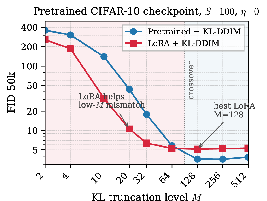
When \(M\) is small, the noise gap \(|\sigma(t) - \sigma_{\!M}(t)|\) is large and the pretrained denoiser is mismatched. LoRA [39] with rank \(r\!=\!4\) efficiently adapts the model to the KL noise schedule. This experiment intentionally uses PFDiff-790k: the goal is to test whether KL-Diffusion can benefit from existing pretrained models rather than requiring training from scratch. 6 (raw values in Supplementary Table VI) shows that LoRA dramatically improves FID for \(M \leq 64\) (up to 77% at \(M\!=\!10\)) but hurts for \(M \geq 128\) where the pretrained model is already well-matched, with crossover between \(M\!=\!64\) and \(M\!=\!128\).
4.6.0.1 Adaptation analysis
The crossover has a clean interpretation. For large \(M\), \(\sigma_{\!M}\!\approx\!\sigma\) (1) and the pretrained denoiser is already well-calibrated, so LoRA’s extra parameters add a residual bias (FID floors near \(5.1\) vs.\(3.6\) unmodified). For small \(M\) the gap \(|\sigma-\sigma_{\!M}|\) is large (\(0.048\) at \(M\!=\!20\), \(0.091\) at \(M\!=\!10\)) and the denoiser overestimates noise; LoRA learns a low-rank bias toward the \(\sigma_{\!M}\) scale, giving up to \(4.4\times\) improvement at \(M\!=\!10\). That rank \(r\!=\!4\) (\(<\!0.1\%\) parameters) suffices confirms a low-dimensional correction, consistent with the spectral shift having rank \(\leq M\).
4.7 Additional Support: Inverse Problem Solving↩︎
To test whether the KL truncation remains useful outside unconditional generation, we plug the same KL noise schedule into Decoupled Annealing Posterior Sampling (DAPS) [40] and evaluate the nonlinear FFHQ-\(256\) phase-retrieval task. Given a clean image \(x_0\) and a noisy measurement \(y\), the inverse problem is \[y = \mathcal{A}(x_0) + n, \qquad n \sim \mathcal{N}(0,\beta_y^2 I),\] with the oversampled Fourier-amplitude operator \(\mathcal{A}(x) = |\mathcal{F}(\operatorname{Pad}(x))|\), oversampling ratio \(2.0\) and \(\beta_y = 0.05\), matching the DAPS paper. Posterior sampling targets \(p(x_0 \mid y) \propto p(y \mid x_0)\,p_{\theta}(x_0)\). KL-DAPS keeps the DAPS reconstruction pipeline unchanged and only replaces the Brownian marginal scale by our KL scale from 6 , namely \(x_t^{(M)} = \alpha(t)\,x_0 + \sigma_M(t)\,\epsilon\) with \(\epsilon \sim \mathcal{N}(0,I)\), so the annealing schedule now follows the \(M\)-truncated variance \(\sigma_M(t)^2\) instead of the original \(\sigma(t)^2\).
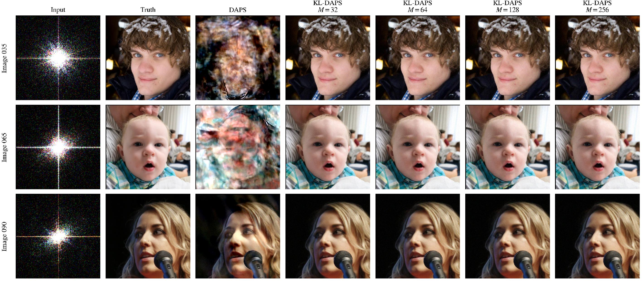
We use the 100-image FFHQ-\(256\) validation subset and the paper-style best-of-four protocol for phase retrieval, applied identically to DAPS and KL-DAPS. As shown in 7, KL-DAPS improves the reproduced DAPS baseline for all tested \(M \in \{32,64,128,256\}\), with \(M=32\) best overall; the differences across \(M\) are small. This setting improves PSNR from \(29.95\) to \(30.68\) (+0.73 dB), SSIM from \(0.774\) to \(0.815\), and LPIPS from \(0.178\) to \(0.152\). The visual comparison in 7 shows the same trend: KL-DAPS recovers cleaner facial structure than the reproduced DAPS baseline across representative examples, with \(M=32\) typically the sharpest setting. This additional inverse-problem experiment supports the same conclusion as the generative benchmarks: a finite intermediate KL truncation can provide a better effective noise schedule than the original Brownian process even when the diffusion prior is used inside a posterior sampler.
| Method | \(M\) | PSNR\(\uparrow\) | SSIM\(\uparrow\) | LPIPS\(\downarrow\) |
|---|---|---|---|---|
| DAPS [40] | — | 29.95 | 0.774 | 0.178 |
| KL-DAPS | 32 | |||
| KL-DAPS | 64 | 30.56 | 0.800 | 0.159 |
| KL-DAPS | 128 | 30.67 | 0.799 | 0.159 |
| KL-DAPS | 256 | 30.44 | 0.791 | 0.165 |
4pt
4.8 Alternative Expansion: Lévy–Ciesielski (LC)↩︎
The KL expansion uses cosine eigenfunctions \(\{\psi_m\}\) because they are optimal in the \(L^2\) sense—they minimize the mean-square truncation error for any given \(M\) (3.1) [25]. A natural question is whether other complete orthonormal bases yield comparable results.
4.8.0.1 LC construction
The Lévy–Ciesielski (LC) construction represents Brownian motion using the Haar wavelet (Schauder) basis. An \(N\)-level LC expansion uses \(M_{\mathrm{eff}} = 2^{N+1}\) basis functions organized by dyadic resolution levels. At level \(N\!=\!7\) (\(M_{\mathrm{eff}}\!=\!256\)), the LC expansion gives a marginal variance \(\sigma_{\mathrm{LC}}^{(N)}(t)\) that converges to \(\sigma(t)\) in a piecewise-linear fashion. The resulting LC samplers (LC-Euler, LC-DDIM, LC-DPM) are defined analogously to their KL counterparts, replacing \(\sigma_{\!M}(t)\) with \(\sigma_{\mathrm{LC}}^{(N)}(t)\); the explicit LC coefficients and sampler updates are given in Supplementary App. A.
4.8.0.2 Results
8 compares KL and LC samplers. The LC variants consistently improve over the DDIM/DPM baselines, confirming that finite-dimensional noise truncation itself is beneficial. The better basis, however, depends on the solver order. For the first-order DDIM update KL is clearly superior (at \(M_{\mathrm{eff}}\!=\!128\), KL-DDIM FID = 5.07 vs. for LC-DDIM, a \(10\%\) gap); for the second-order DPM-O2 solver the two bases fall within a few percent, with Haar marginally ahead (at \(M_{\mathrm{eff}}\!=\!256\), LC-DPM O2 3.94 vs. for KL-DPM O2). A 3-seed check places both effects outside seed noise.
| Sampler | Basis / \(M_{\mathrm{eff}}\) | FID-50k |
|---|---|---|
| DDIM | — | 6.90 |
| DPM-O2 | — | 4.61 |
| KL-DDIM | KL / 128 | |
| LC-DDIM | LC / 128 (\(N\!=\!6\)) | 5.66 |
| KL-DPM O2 | KL / 256 | 4.11 |
| LC-DPM O2 | LC / 256 (\(N\!=\!7\)) |
4pt
4.8.0.3 KL vs.LC: basis meets solver order
The KL expansion is the unique \(L^2\)-optimal basis [8]: its eigenfunctions \(\psi_m(t)\) are adapted to the SDE covariance through \(c_m(t)\), so truncation drops the least energetic modes first, whereas the Haar basis spreads approximation power uniformly across dyadic scales regardless of the schedule. This optimality is visible at first order, where KL-DDIM beats LC-DDIM. At second order (DPM-O2) the solver’s own discretization error dominates the residual basis gap and the two bases become comparable (Haar marginally ahead). We therefore adopt KL for its \(L^2\)-optimality and its consistent first-order advantage, rather than for a universal dominance over Haar.
Additional \(S\)-sweep curves and representative sample grids are reported in Supplementary Apps. B and C.
5 Conclusion↩︎
A pretrained diffusion model operates below its prescribed noise level—a counterintuitive mismatch with the matched-marginal assumption of diffusion. We addressed it with KL-Diffusion: truncating the Karhunen–Loève expansion of the Brownian driver yields a finite-dimensional forward process, a KL training loss, and a family of KL samplers, all governed by a single truncation order \(M\) that dials the noise level independently of the step count \(S\).
The central object is the effective mode count \(M^*\). A finite-capacity denoiser, fit on finitely many samples, behaves as the MMSE denoiser at a reduced level \(\sigma_{\mathrm{eff}}(t)<\sigma(t)\); a closed-form \(2\)-Wasserstein analysis then puts a unique interior optimum on any pointwise-monotone family of reduced schedules, and \(M^*\) is read off a one-dimensional sweep. This single quantity unifies the two uses of the framework. On the sampling axis, KL samplers probe \(M^*\) on fixed checkpoints and improve them without retraining—across CIFAR-10, CelebA, ImageNet \(64\!\times\!64\) and Stable Diffusion v1.4, and across formula-based (DDIM, DPM-Solver) and learned-predictor (AMED) solvers—with the optimal order varying but the U-shape invariant. On the training axis, a controlled CIFAR-10 study shows that training-side and sampling-side sweeps recover the same \(M^*\), and that training at \(M'\!=\!M^*\) gives the best-matched pipeline (\(2.8\times\) faster convergence and lower final FID); iterating the match defines a descending-\(M^*\) procedure, reported as an empirical heuristic.
Limitations and open questions.
Our generative evaluation centres on FID (complemented by PSNR/SSIM/LPIPS for the inverse problem); most reported values are single-run, with 1 giving the three-seed spread, so our conclusions rest on the shape of full sweeps rather than on isolated pairwise differences. The Gaussian analysis controls second moments only, and \(M^*\) is located by a per-configuration sweep. Open questions include a convergence analysis of the descending-\(M^*\) procedure, why the swept order depends on the sampler and why the basis advantage narrows at higher solver order, multi-time KL training objectives, and extensions to other (and non-SDE) generative processes.
6 Verification of Convergence↩︎
Throughout we adopt the normalization \(T=1\) (the general case follows by time rescaling) and use the exact representation 4 of 3.1 together with its derivative eigenfunctions 3 , which at \(T=1\) read \(\psi_m(t)=\sqrt{2}\cos\!\big((m-\tfrac12)\pi t\big)\), with coefficients \(c_m(t):=\int_0^t h\,\psi_m\,\mathrm{d}s\). All results extend coordinate-wise to \(\mathbb{R}^d\) with \(\mathrm{Var}[X_t^{(M)}]=\sigma_{\!M}^2(t)\,I_d\).
Theorem 2 (Convergence of KL-diffusion). Assume \(h \in C^1([0,1])\). Then:
\(\mathbb{E}[|X_t - X_t^{(M)}|^2] = \alpha(t)^2\sum_{m>M} c_m(t)^2 \to 0\) for each \(t\).
\(\sup_{t \in [0,1]} \mathbb{E}[|X_t - X_t^{(M)}|^2] \to 0\).
\(\sup_{t \in [0,1]} \mathbb{E}[|X_t - X_t^{(M)}|^2] \leq C/M\) where \(C = (\max_t \alpha(t))^2 \cdot A^2/\pi^2\) and \(A = \sqrt{2}(\|h\|_\infty + \|h'\|_\infty)\).
Proof. By 4 and 5 the error is \(X_t - X_t^{(M)} = \alpha(t)\sum_{m>M} c_m(t)\,Z_m\), and since the \(\{Z_m\}\) are independent \(\mathcal{N}(0,1)\), \(\mathbb{E}[|X_t - X_t^{(M)}|^2] = \alpha(t)^2 \sum_{m>M} c_m(t)^2\).
(i) Pointwise. Parseval’s theorem gives \(\sum_{m\ge1} c_m(t)^2 = \int_0^t h(s)^2\,\mathrm{d}s < \infty\), so the tail \(\sum_{m>M} c_m(t)^2 \to 0\).
(ii)–(iii) Uniform rate. We bound \(c_m\) by integration by parts. With \(\psi_m(s)=\sqrt{2}\cos(\omega_m s)\), \(\omega_m=(m-\tfrac12)\pi\) (from 3 at \(T=1\)), and \(u=h(s)\), \(\mathrm{d}v=\cos(\omega_m s)\,\mathrm{d}s\), \[c_m(t)=\sqrt{2}\Bigl[\tfrac{h(t)\sin(\omega_m t)}{\omega_m} -\tfrac{1}{\omega_m}\!\int_0^t\! h'\sin(\omega_m s)\,\mathrm{d}s\Bigr],\] the boundary term at \(0\) vanishing. Using \(|\sin|\le1\) and \(t\le1\), the two pieces are at most \(\|h\|_\infty/\omega_m\) and \(\|h'\|_\infty/\omega_m\), so \[\label{eq:cm-bound} |c_m(t)|\le\frac{\sqrt{2}\,(\|h\|_\infty+\|h'\|_\infty)}{\omega_m}=\frac{A}{\omega_m},\tag{24}\] with \(A:=\sqrt{2}\,(\|h\|_\infty+\|h'\|_\infty)\), for all \(t\in[0,1]\) (finite since \(h\in C^1\)). Squaring and using \((m-\tfrac12)^2\ge(m-1)m\), the tail telescopes: \[\begin{align} \sum_{m>M}c_m(t)^2 &\le\frac{A^2}{\pi^2}\sum_{m>M}\frac{1}{(m-\tfrac12)^2} \le\frac{A^2}{\pi^2}\sum_{m>M}\Bigl(\tfrac{1}{m-1}-\tfrac{1}{m}\Bigr)\\ &=\frac{A^2}{\pi^2 M}. \end{align}\] Multiplying by \(\alpha(t)^2\le(\max_t\alpha(t))^2\) and taking the supremum gives \(\sup_t\mathbb{E}[|X_t-X_t^{(M)}|^2]\le C/M\) with \(C=(\max_t\alpha(t))^2 A^2/\pi^2\), which is (iii); (ii) follows since \(C/M\to0\). ◻
7 Uniform-Angle Estimate of \(\kappa_S\)↩︎
The discretization factor 13 is the supremum of the \(S\)-fold cosine product at fixed total sweep \(\Phi=\phi(t_S)\), \(\kappa_S=\sup\{\prod_{k=1}^{S}\cos\delta_k:\delta_k\ge0,\;\sum_{k}\delta_k=\Phi\}\). Since \(\log\cos\) is concave on \([0,\tfrac{\pi}{2})\), Jensen’s inequality makes the product largest at equal angles \(\delta_k=\Phi/S\), so, using \(\log\cos\delta=-\delta^2/2-\delta^4/12-\cdots\), \[\label{eq:kappa-uniform} \begin{align} \kappa_S=\cos^S\!\Big(\frac{\Phi}{S}\Big) &=\exp\!\Big(-\frac{\Phi^2}{2S}-\frac{\Phi^4}{12S^3}-\cdots\Big)\\ &=e^{-\Phi^2/(2S)}\big(1+O(S^{-3})\big). \end{align}\tag{25}\] The deficit is \(O(1/S)\): doubling the number of steps roughly halves \(1-\kappa_S\). For \(\Phi=\pi/2\), \(S=20\) this gives \(\kappa_S\approx e^{-\pi^2/160}\approx0.94\).
References↩︎
Y. Ren, Y. Liu, A. Artola, and L. Mertz are with City University of Hong Kong. J.-M. Morel and R. H. Chan are with Lingnan University of Hong Kong.↩︎