MAME: Multidimensional Adaptive Metamer Exploration with
Human Perceptual Feedback
March 17, 2025
Keywords: metamers; texture synthesis; psychophysics; cognitive neuroscience; machine learning
1 Introduction↩︎
2 Methods↩︎
3 Results↩︎
4 Discussion↩︎
5 Conclusions↩︎
6 Acknowledgments↩︎
This work was supported by JSPS KAKENHI Gran Numbers JP21H04909 and JP26K02927. We used ChatGPT (OpenAI) for English language editing. All content was reviewed and verified by the authors.
7 Supplementary Materials↩︎
![Figure 1: Examples of image modulation using models with different training regimes but the same architecture as the robust ResNet50 used in this study. The robust ResNet was trained to be resistant to adversarial attacks, whereas the default model was trained on standard ImageNet data, and the stylized model was trained on stylized versions of ImageNet [1]. When the same modulation parameters were applied to each model, we found that, particularly in higher layers, the default and stylized models failed to produce clear modulations from the original image, in contrast to the robust model (cf. Feather, 2023).](/article/2503.13212/figures/model_compare.png "fig:")
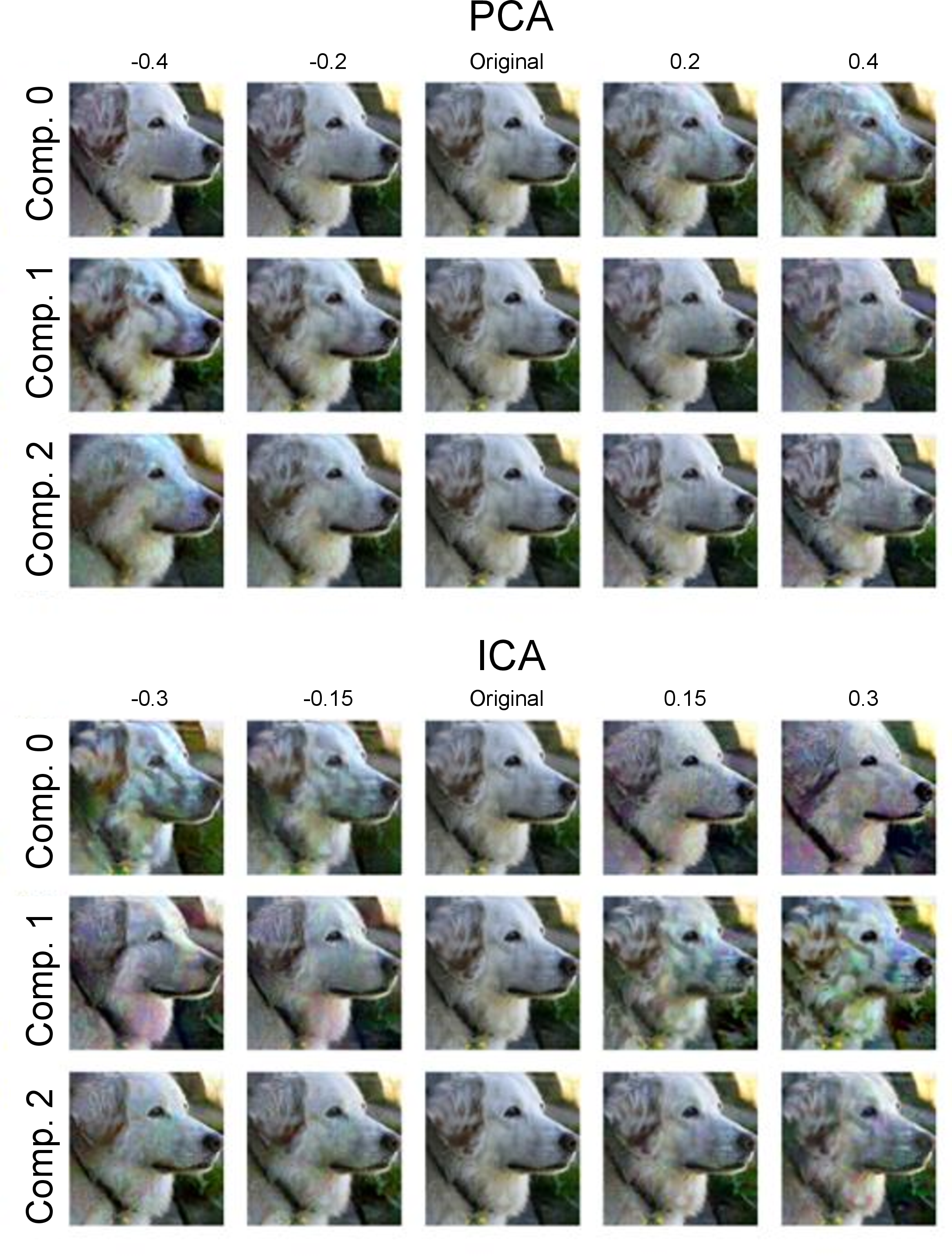
![Figure 3: Examples of image modulation for each layer and each component. This figure presents a finer-step version of Fig. [fig:imggen_examples].](/article/2503.13212/figures/figure_s3.png "fig:")
| Layer | \(\log_{10}(t)\) range | Component | Direction | Normalized final loss |
|---|---|---|---|---|
| conv1 | [0.0, 3.0] | 0 | + | 0.006636 \(\pm\) 0.024610 |
| \(-\) | 0.007039 \(\pm\) 0.027097 | |||
| 1 | + | 0.004328 \(\pm\) 0.010553 | ||
| \(-\) | 0.004179 \(\pm\) 0.010673 | |||
| 2 | + | 0.005512 \(\pm\) 0.010508 | ||
| \(-\) | 0.007136 \(\pm\) 0.014643 | |||
| layer3 | [-2.0, 1.0] | 0 | + | 0.006004 \(\pm\) 0.012682 |
| \(-\) | 0.005656 \(\pm\) 0.010533 | |||
| 1 | + | 0.007383 \(\pm\) 0.014922 | ||
| \(-\) | 0.006431 \(\pm\) 0.014312 | |||
| 2 | + | 0.005035 \(\pm\) 0.008581 | ||
| \(-\) | 0.006483 \(\pm\) 0.011846 | |||
| avgpool | [-2.0, 1.0] | 0 | + | 0.013961 \(\pm\) 0.055785 |
| \(-\) | 0.011262 \(\pm\) 0.044577 | |||
| 1 | + | 0.006213 \(\pm\) 0.021678 | ||
| \(-\) | 0.007241 \(\pm\) 0.016612 | |||
| 2 | + | 0.008365 \(\pm\) 0.026241 | ||
| \(-\) | 0.006456 \(\pm\) 0.017010 |
| Layer | Eccentricity (°) | Mean | Std |
|---|---|---|---|
| conv1 | 4 | 47.915 | 8.8166 |
| 8 | 63.0404 | 11.8613 | |
| 12 | 63.7918 | 8.5024 | |
| layer3 | 4 | 0.486 | 0.1275 |
| 8 | 0.5983 | 0.0686 | |
| 12 | 0.6407 | 0.0533 | |
| avgpool | 4 | 0.1538 | 0.0182 |
| 8 | 0.153 | 0.0253 | |
| 12 | 0.1688 | 0.0203 |
| Source | df | \(F\) | \(p\) | \(\eta_g^2\) | |
|---|---|---|---|---|---|
| Layer | \((2, 14)\) | 696.67 | \(< .001\) | 0.936 | |
| Eccentricity | \((2, 14)\) | 30.91 | \(< .001\) | 0.346 | |
| Layer \(\times\) Eccentricity | \((4, 28)\) | 7.00 | .016 | 0.218 |
| Source | df | \(F\) | \(p\) | \(\eta_g^2\) | |
|---|---|---|---|---|---|
| Layer | \((2, 14)\) | 826.47 | \(< .001\) | 0.937 | |
| Eccentricity | \((2, 14)\) | 38.25 | \(< .001\) | 0.368 | |
| Layer \(\times\) Eccentricity | \((4, 28)\) | 5.30 | .044 | 0.183 |
| Source | df | \(F\) | \(p\) | \(\eta_g^2\) | |
|---|---|---|---|---|---|
| Layer | \((2, 14)\) | 1871.61 | \(< .001\) | 0.980 | |
| Eccentricity | \((2, 14)\) | 23.16 | \(< .001\) | 0.316 | |
| Layer \(\times\) Eccentricity | \((4, 28)\) | 8.47 | .015 | 0.248 |
References↩︎
[1]
R. Geirhos, P. Rubisch, C. Michaelis, M. Bethge, F. A. Wichmann, and W. Brendel, “ImageNet-trained CNNs are biased towards texture; increasing shape bias improves accuracy and
robustness,” arXiv preprint arXiv:1811.12231, 2018.
Corresponding authors: Masataka Sawayama and Mina Kamao↩︎