1 Introduction↩︎

The efficient simulation of stochastic systems is a cornerstone of many critical applications, ranging from rare-event estimation to gradient estimation in Reinforcement Learning. In many practical scenarios, the underlying dynamics of a system are complex, poorly characterized, or entirely unknown, placing us essentially in a model-free setting. In such contexts, strategies for exploring the state space where the stochastic dynamics live and gathering informative samples are paramount. This work investigates two powerful and general mechanisms for enhancing the efficiency of stochastic simulations: parallelization and restarting. We aim to provide a rigorous probabilistic analysis of these strategies, with applications focused on key model-free problems such as estimating small probabilities for stochastic processes with unknown dynamics and the challenge of efficient exploration in Reinforcement Learning (RL).

A canonical problem in probability and statistics is the estimation of the probability that a stochastic process reaches a rare, distant state within a finite time horizon. Standard Monte Carlo methods fail as the event of interest is rarely observed. A common technique for accelerating rare event simulation is importance sampling, [1] which involves simulating the process under an alternative “twisted" measure that makes the rare event more likely, and then correcting this change of measure via likelihood ratios. However, importance sampling is not a viable solution in the model-free settings as its application requires exact knowledge of the underlying process dynamics to construct the optimal change of measure. When the dynamics are unknown or too complex to model — as is often the case in large-scale RL environments or with intractable stochastic processes—this precise knowledge is unavailable, rendering importance sampling inapplicable. Moreover, an estimation scheme for the change of measure is usually of very large variance. It is precisely this limitation that motivates the use of blind or model-free strategies, such as parallelization and restarting, which do not require explicit knowledge of the system dynamics.

Parallelization—running multiple independent simulations concurrently—seems a natural remedy, as it increases the chances of observing the rare event. However, under a fixed total computational budget, a critical trade-off emerges: should one allocate the entire budget to a single, long simulation, or distribute it among many shorter, parallel runs? The answer is not trivial, as splitting the budget too finely may deprive each simulation of the necessary time to reach the rare state. We analyze this trade-off quantitatively, identifying a sharp phase transition in the success probability as a function of the number of parallel runs.

Beyond parallelization, restart strategies offer another avenue for improvement. Instead of letting simulations run in potentially unfruitful regions of the state space, a restart mechanism halts them and re-initializes them from more promising states, effectively redirecting computational effort. This restarting mechanism is particularly powerful in scenarios where certain regions are more likely to lead to the target event. A well-designed restart policy can prevent the waste of resources on trajectories with a low probability of success and serves as a practical, model-free alternative to importance sampling.

Several recent works have addressed the efficient exploration challenge, in particular for RL. For example, the Go-Explore approach in [2] introduces an innovative solution by distinctly separating the exploration and exploitation phases. This method allows the algorithm to maintain a repository of promising states, which can be revisited for further exploration, significantly enhancing the ability to discover and leverage rare or hard-to-reach states. Another example is found in [3] based on the paradigm of Fleming-Viot particle system, introduced by [4]. In this framework, a population of particles (which can represent different simulations in parallel) evolves over time, exploring the state space in parallel. When a particle falls into a less promising region, it is “restarted" by being replaced with a copy of another, more promising particle. This ensures that resources are concentrated on exploring the most fruitful areas of the state space.

Beyond RL, stochastic restarting has been studied extensively across disciplines such as statistical physics, computer science, and network theory, primarily to minimize expected task-completion times modeled via first-passage times (see, e.g., [5]–[7]). In contrast, our work focuses on the asymptotic behavior of the full distribution of passage times, studying large-deviation regimes and rare-event phenomena through asymptotic estimates, bounds, and threshold effects rather than expectations. While related analytic frameworks for Markov processes with restart—addressing ergodicity, quasi-stationary distributions, and connections to Fleming–Viot systems—are developed in [8], our results concern finer asymptotics for more restricted process classes and different probabilistic questions. Our work also differs from [9], which analyzes large deviations for the long-time asymptotics with stochastic restart to a fixed state. In contrast, we consider large deviations with respect to a spatial parameter modeling the complexity of exploring the state space.

Despite the promise of parallel simulation techniques and restart mechanisms, there is a lack of quantitative evidence of their potential benefits. Specifically, the extent to which these strategies improve exploration efficiency and yield better learning outcomes remains unclear. We aim to fill this gap by providing a detailed analysis of the impact of parallel simulations combined with restart mechanisms on the exploration process, modeled as the task of reaching a specific subset of the state space. To achieve this, we use a simplified model based on toy dynamics, specifically random walks and Lévy processes. These processes are chosen for their mathematical tractability and their ability to capture fundamental aspects of the problem, allowing explicit analytical results. Although these dynamics are simple, they provide crucial insights into the mechanisms that govern exploration, forming the basis for future work with more involved Markovian dynamics. By employing this framework, we examine two key aspects of exploration:

• Exploration complexity, encapsulated by a parameter that quantifies the fluctuations necessary to achieve effective exploration and reach the target subset of the state space,

• Exploration diversity, represented by the number of parallel simulations employed, which increases the breadth of the state-space search and enhances the likelihood of encountering rare, high-reward states within the target subset.

We focus our analysis on a specific regime where the exploration complexity scales linearly with the simulation budget. The toy dynamics framework allows us to examine these parameters within finite time budgets systematically and to quantify how parallel simulations improve efficiency by leveraging diversity, while restarting mechanisms enable particles to avoid stagnation by redirecting effort toward more promising regions of the state space, ultimately facilitating the achievement of the exploration goal.

Our approach relies on the systematic analysis of these strategies under finite time budgets, using analytical techniques based on exponential martingales to quantify the effects of parallel simulations and restarting mechanisms. By addressing the interplay between exploration diversity and the power of parallelization and restarting mechanisms, our work provides novel insights into efficient exploration strategies and lays the groundwork for further investigations into more complex stochastic dynamics.

Through this investigation, our goal is not only to demonstrate the potential utility of these techniques but also to delineate their limitations. Understanding these nuances is crucial for developing more efficient stochastic simulations in model-free settings such as RL, particularly in environments characterized by sparse rewards. Ultimately, our findings aim to provide actionable insights into when and how to leverage parallel simulations and restarting strategies to optimize exploration, thereby advancing the field in both theory and practice.

Problem Statement and Contributions↩︎

In this work, we model exploration as a one-dimensional stochastic process, often referred to as a particle, aiming to reach a target subset of the state space. This target, represented as a barrier, captures a potentially informative state that is difficult to attain, making it essential to devise strategies that maximize the probability of success within a finite time budget and to quantify the resulting improvements. In the following we summarize our main findings and key take-away messages.

1. Phase Transition in Reaching Probabilities. We identify a striking phase transition in the probability of reaching the target subset of the state space as a function of the number of parallel simulations \(N\). In Theorems 1 and 2, we rigorously show that when the time budget scales linearly with the barrier level, there is a sharp transition in performance. Our analysis is based on large deviations techniques and the transition happens at a certain threshold which we present explicitly. Below this threshold, concentrating the entire budget on a single particle is optimal. If the budget, when split into \(N\) parts, remains above the threshold, then distributing it among \(N\) particles significantly improves the probability of success. However, using too many particles—thereby reducing the time available to each beyond the threshold—results in exponentially diminished performance.

2. Optimal Number of Parallel Simulations. In view of the previous point, a critical contribution is then the determination of an optimal number of parallel simulations, \(N^*\), that balances the trade-off between exploration diversity and the time allocated to each particle. This optimal \(N^*\) depends intricately on the time budget and the large deviations characteristics of the particles dynamics, but in terms of the phase transition mentioned above it can be characterized as the largest integer for which the split budget exceeds the threshold.

3. Exponential Boost via restarting strategy. To overcome stagnation and improve the probability of reaching the target, we introduce a restarting mechanism inspired by mechanisms described, for instance, in [3]. We study an idealized situation in which this mechanism replaces particles with a low likelihood of success and restarts them at new initial positions sampled from a given measure. Our theoretical results (Theorem 3) demonstrate that this restarting strategy can substantially enhance the probability of success. The improvement is quantified by a factor proportional to the time budget and the exponential moments of the measure associated with the restarting mechanism. A particularly interesting restarting measure is a quasi-stationary distribution (QSD) over a set representing high-probability regions for successful trajectories. For these restarting measures, we can obtain sharper asymptotics using different methods that exploit the QSD properties. We note that this restarting strategy can be well approximated in practice by selection mechanisms such as the Fleming-Viot or Aldous-Flanary-Palacios algorithms (see [10] and the references therein). These schemes enable practical implementation and adequate sampling of initial positions, making the restarting mechanism computationally feasible in real-world scenarios.

   Finally, from a practical point of view, we present contributions in two directions for queueing systems. The first one corresponds to the problem of estimating small probabilities. We analyze the interplay between the probability of exploration and the efficiency of the associated estimation method. For the particular case of an M/M/1 queue, we show that the variance of the vanilla Monte Carlo estimator is essentially determined by the typical exploration time. The second, with broader impact, addresses efficient exploration in RL. In RL environments with sparse rewards, the core of the efficient exploration challenge lies in the inability of algorithms such as policy gradient methods to perform effective policy updates (see [2] and references therein). These methods estimate the gradient of the expected return with respect to the policy parameters. This estimation relies crucially on exploring the state space; if the agent fails to reach rewarding states, the gradient estimates are biased and ineffective. Our work addresses this specific issue: we aim to improve gradient estimation (hence policy evaluation under a fixed policy) not by changing the policy, but by enhancing the exploration process used to evaluate it. The M/M/1/K queue considered in [3] is reanalized here to illustrate our results.

Organization of the paper↩︎

In Section 2, we introduce the models for the exploration process, which represent the dynamics of the exploration phase in RL. Like the rest of the paper, this section is divided into two parts. The first part analyzes the effects of parallel exploration, and the second part analyzes our restarting mechanism. Section 3 presents our main results for the two scenarios described above, after some necessary preliminaries. Main results are discussed in generality and illustrated through numerical simulations for concrete instances. In Section 4, we prove Theorems 1 and 2 related to parallel exploration. In Section 5 we prove Theorem 3 for exploration with a general restarting measure and in Section 6 we prove Theorem 4 for a QSD restarting measure. Finally, appendices are devoted to practical applications of our work.

2 Exploration strategies↩︎

We now formally introduce the models for exploration, using random walks and Lévy processes as simplified toy models. We focus on the probability of reaching a distant state \(x\) from an initial position of \(0\), with the drift component encoding the difficulty of exploration. The drift represents the inherent challenge in progressing towards the target state, where a stronger drift away from the target reflects a more difficult exploration task.

We consider scenarios where the total time budget scales with \(x\), allowing us to examine how exploration strategies perform as the target’s reaching difficulty increases. Two specific strategies are explored: the first investigates parallel exploration under a fixed time budget, while the second examines the effects of restarting the process when it crosses a predefined threshold. Although these models are simplified, they provide critical insights into the fundamental principles that govern the effectiveness of exploration strategies in RL, particularly in challenging environments where reaching an unlikely target state is the goal.

2.1 Strategy I: parallel exploration.↩︎

Let \(\{Z_i(t)\}_{t\in I}, i \in \{1,\dots,N\}\), where \(I= \mathbb{N}\) or \(I= \mathbb{R}^+\), be a family of one-dimensional random walks or Lévy processes. Define further \[\begin{align} \tau_i(x) &\coloneq \inf \{ t\in I:\;\;Z_i(t) \ge x\}, \\ \tau^{(N)}(x)& := \min \{ \tau_1(x), \tau_2(x), \dots, \tau_N(x) \}, \label{def:tau} \end{align}\tag{1}\] the time it takes particle \(i\) to reach state \(x\), and the first time one of \(N\) particles reaches \(x\), respectively.

First, the case of \(N\) parallel independent simulations is analyzed. We introduce as performance criterion for exploration the probability that starting from \(0\), one of the simulations reaches the rare state \(x\) within a given time budget \(B(x)/N\), i.e. \[\PP\Big( \tau^{(N)}(x) \leq B(x)/N \Big).\]

We aim at characterizing this probability (as a function of \(N\)) in the regime where the total simulation budget, \(B(x)\), satisfies \(x = C\cdot B(x) + o \left(\sqrt{B(x)}\right)\), for \(x\) large and \(C\) some positive constant. This is the focus of Theorem 1 for random walks and Theorem 2 for Lévy processes.

2.2 Strategy II: exploration with restart.↩︎

Our second model incorporates a restart mechanism into the dynamics of a random walk or a Lévy process. The ingredients of the model are: a positive number \(x>0\) (the rare state we want the process to reach), a probability measure \(\nu_x\) supported on \((0,x)\), and a discrete random walk or a Lévy process \(Z = \{Z(t)\}_{t\in\RR^+}\). The trajectories of the process under study can be viewed as a concatenation in time of independent and identically distributed cycles, each consisting of sampling a state \(y_0\) from \(\nu_x\) and simulating the trajectory of \(y_0+Z(t)\) until the first time it exits the interval \((0,x)\).

Our goal is to analyse the first passage time over \(x\) of the restarted process, and compare it with the corresponding one for the process without restart. The conditions required on the family of restart measures to improve algorithmic performance are quite general. Essentially, it suffices that each \(\nu_x\) be stochastically dominated by a non-degenerate measure possessing a finite second moment. We also examine in detail the case where restart occurs according to the unique quasi-stationary measure of the process \(Z\) absorbed at \(\RR^+\setminus (0,x)\) (see Section 3.4 for precise definitions). Our motivation for this particular mechanism (restarting from quasi-stationary distributions) is that the resulting process approximates complex particle dynamics built upon a given Markov process, a key example, as noted earlier, being the class of Fleming–Viot particle systems. Our model is indeed an approximation of the Fleming-Viot dynamics since the stationary distribution of the \(N-\) particle system approximates the quasi-stationary distribution associated with the underlying Markov process absorbed upon reaching \(A\), as \(N\) goes to infinity (see Appendix II for more details).

3 Main results↩︎

After introducing due notation, we present our results for each strategy.

3.1 Parallel exploration driven by a random walk↩︎

Let \(Z(t) = X_1+\dots+X_t\), \(t\in\NN\) be a random walk with independent increments all distributed as a random variable \(X\). We will always assume that \(X\) is not deterministic, meaning that it is not concentrated on a single value, and that it may take both positive or negative values with positive probability. The moment-generating function (mgf) of \(X\), \(\varphi(\lambda):= \EE[\exp(\lambda X)]\), is strictly convex on the interior points of the set \(\Lambda\) (\(\text{int}(\Lambda)\)) where \(\Lambda := \{\lambda\in \RR:\;\varphi(\lambda) <+\infty\}.\) The following condition is usually referred to as the right Cramér condition: \[\label{right95cramer95cond} \Lambda_+ := (0,+\infty)\cap \text{int}(\Lambda)\;\textit{is non empty,}\tag{2}\] We will work under further additional assumptions: \[\label{diff95mgf} \textit{ \varphi is at least twice differentiable in } \Lambda_+,\tag{3}\] and \[\label{positive95cramer95exp} \textit{There exists } \lambda^* \in \Lambda_+:\;\psi(\lambda^*) = 0 \quad \text{ where } \quad \psi(\lambda)\mathrel{\vcenter{:}}= \log \varphi(\lambda)\tag{4}\]

Note that \(\EE[X] = \psi'(0)\) and assumptions 2 , 3 and 4 imply that \(\EE[X] < 0\) and \(\psi'(\lambda^*) > 0\), since \(\psi(\lambda^*) = \psi(0)\) and \(\varphi\) is strictly convex. Let \(\tau(x)\) denote the first time the random walk reaches level \(x\), defined as: \[\label{def:passage95time} \tau(x) := \inf\{ t \geq 0 : Z(t) \geq x \}.\tag{5}\] Furthermore, let \(\tau^{(N)}(x)\) represent the minimum of \(N\) independent random times, each distributed as \(\tau(x)\), i.e., \[\label{def:min95of95passage95times} \tau^{(N)}(x) := \min \{ \tau_1(x), \tau_2(x), \dots, \tau_N(x) \},\tag{6}\] which corresponds to the first time any of \(N\) independent random walks reaches level \(x\).

Our first main theorem states that the interesting behaviour of \(\tau(x)\) and \(\tau^{(N)}(x)\) occurs while comparing them to functions of the following classes: for \(\lambda\in\Lambda_+\) let \[\label{def:asymp95linear95funcs} L(\lambda) \mathrel{\vcenter{:}}= \left\{f:\RR\to\RR\;\text{ such that } x = \psi'(\lambda)\cdot f(x) + \boldsymbol{o}\left(\sqrt{f(x)}\right)\;\text{as } x\to+\infty\right\}.\tag{7}\] This set consists of functions \(f(x)\) that asymptotically behave like \(x/\psi'(\lambda)\) with an error term of order smaller than \(\sqrt{f(x)}\). The result below is stated for the class of functions defined above but the reader can think of a specific example being \(B(x) = x/\psi'(\lambda)\) for any \(\lambda\in\Lambda_+\).

We now state our main result regarding parallel exploration for random walks:

In the regime in which the theorem is stated, probabilities decay exponentially as \(x\) goes to infinity (see Proposition [thm:estimates95pasasge95times] in Section 4). The result shows that using too many particles (thus giving too little time to each) entails an exponentially worse performance, meaning that \(\PP\left(\tau^{(N)}(x)\leq \frac{B(x)}{N}\right)\) decays with a faster exponential rate than \(\PP\left(\tau(x)\leq B(x)\right)\). On the other hand using too few particles comes only at a linear cost in performance.

The main intuition behind the results stated above is that within the (rare) event \(\{\tau(x) < +\infty\}\), the probability is concentrated on those trajectories with drift \(\psi'(\lambda^*)\), for which the time needed to reach \(x\) is \(\tau(x) \approx x/\psi'(\lambda^*)\). This idea is formalized using exponential martingales and is at the core of Proposition [thm:estimates95pasasge95times]. Our results show that allowing a budget smaller than \(x/\psi'(\lambda^*)\) substantially reduces the probability of success, while allowing too much budget results in no significant improvement. In the latter case, by splitting it into several independent particles, each one provides an “extra chance" of success.

Even though in general \(\lambda^*\) and (thus) the threshold \(\psi'(\lambda^*)^{-1}\) depend in a non-trivial way on the distribution of the increments, in some cases it is possible to find simple expressions for these parameters. We present some of the important examples here.

3.1.1 Simulations for parallel random walks:↩︎

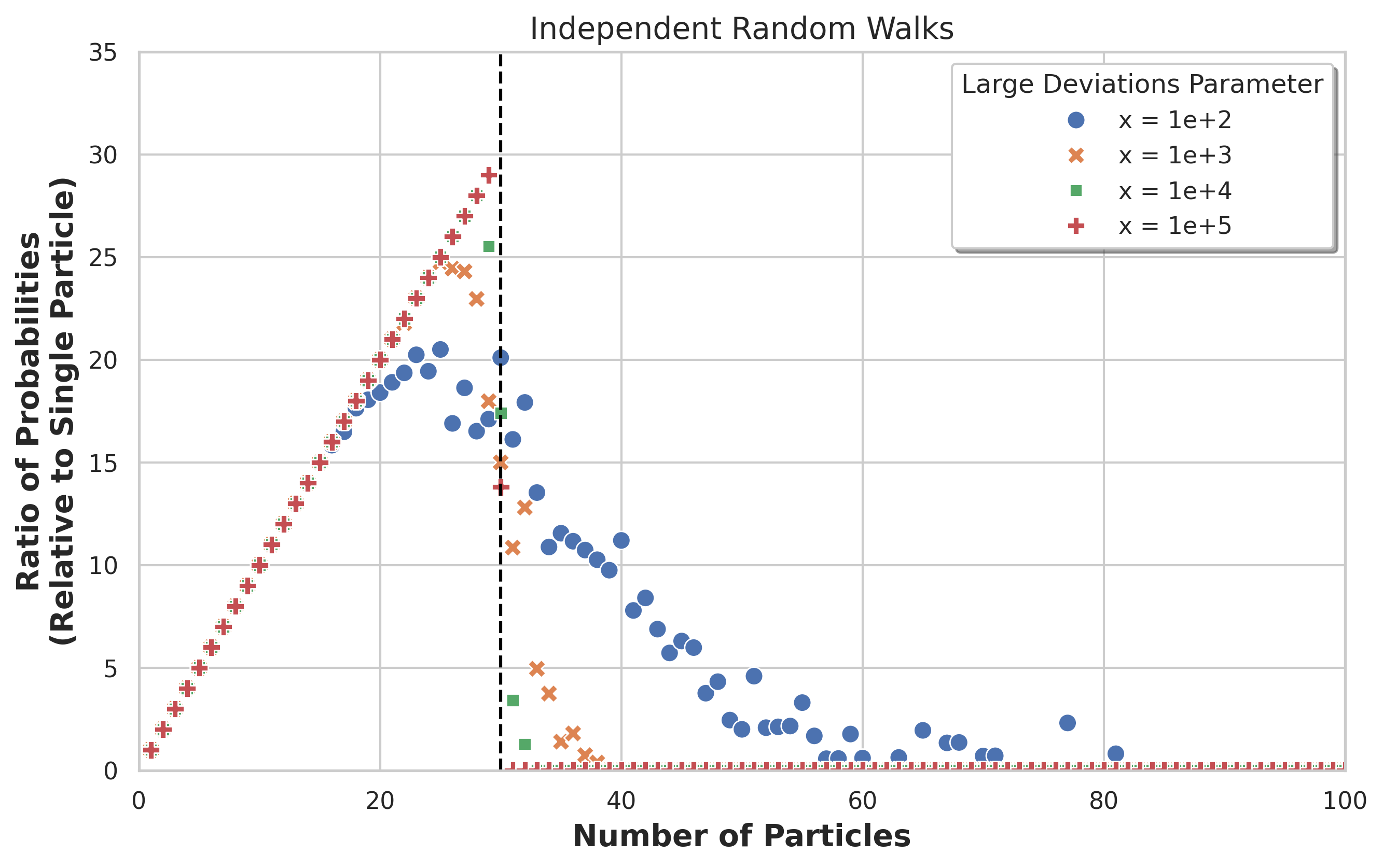
Consider the random walk case described in Example 2. We use the parameters \(p=0.45\) and \(B(x)=300\cdot x\), which imply \(\psi'(\lambda^*)=0.1\). According to Theorem 1 the ratio \[\label{eq:quotient95parallel95exp} \frac{\PP\left(\tau^{(N)}(x)\leq \frac{B(x)}{N}\right)}{\PP\left(\tau(x)\leq B(x)\right)}\tag{8}\] is expected to approach the identity for \(N< 300\cdot 0.1=30\) and zero for \(N>30\), as \(x\to\infty\). This is the behaviour observed in Figure 1.

For the simulation we used the measure \(\PP^{\lambda^*}\) as defined in 12 , under which the process is distributed as a birth-and-death random walk with interchanged parameters, namely \(p^* = \PP^{\lambda^*}(X_1 = 1) =1-\PP^{\lambda^*}(X_1 = -1) = 1-p\). Under this measure, passage over a given \(x\in\NN\) is not a rare event anymore so simulations are feasible. For each large deviation parameter \(x\in\{20,100,500,1000,2500\}\), and for each number of particles \(N\) between \(1\) and \(100\) we simulate and average over \(1000\) random walks to get an estimate of \(\PP^{\lambda^*}(\tau \leq B(x)/N)\). By reverting the measure change we obtain estimates for the original ratio.

3.2 Parallel exploration driven by a Lévy process↩︎

Random walks have an analogue in continuous time known as Lévy processes. Under analogous assumptions on the exponential moments, we can extend Theorem 1 to the case of Lévy processes on \(\mathbb{R}\). This is based on the fact the asymptotics for first passage times over high barriers are similar in the cases of random walks and Lévy processes, see Section 4. We now review some preliminaries on Lévy processes, all of which may be found in classical references such as [11] and [12].

Let \((\Omega,\cF,\{\cF_t\}_t,\PP)\) be a filtered probability space, where the filtration \(\{\cF_t\}_t\) is assumed augmented and right-continuous. A Lévy process \(Z = \{Z(t)\}_{t\in I}\), \(I=[0,+\infty)\) is a stochastic process such that for all \(0\leq s\leq t\), \(Z(t)\) is \(\cF_t\) measurable, \(Z(0)=0\), \(Z(t)-Z(s)\) is independent of \(\cF_s\) and has the same distribution as \(Z(t-s)\), and is continuous in probability, namely that \(Z(t+s)\to Z(t)\) in probability if \(s\to 0\). We will always work with a cádlàg version of \(Z\). Let \(\psi\) denote the Lévy exponent of \(Z\): \[\EE e^{\lambda Z(t)} = e^{t\psi(\lambda)}.\] The Lévy-Khintchine formula introduces the characteristic triplet \((-\mu,\sigma,\Pi)\) of \(Z\): \[\label{eq:levy95exponent} \psi(\lambda) = \log \EE e^{\lambda Z(1)} = -\mu \lambda + \frac{(\sigma\lambda)^2}{2} + \int_{-\infty}^{+\infty} (\exp(\lambda y)-1 - \lambda y \bfone(|y|\leq 1))\Pi(dy);\tag{9}\] where \(\mu\in\RR\) is called the drift coefficient, \(\sigma\in (0,+\infty)\) is the diffusion coefficient (note that we exclude the finite-variation case) and \(\Pi\) is a measure in \(\RR\setminus\{0\}\) such that \[\int_{-\infty}^{+\infty} (1\wedge y^2) \Pi(dy) <+\infty,\] called the Lévy measure (or jump measure). As in the discrete-time case we will work under Cramér’s condition: \(\EE(e^{\lambda Z(1)})\) is finite for \(\lambda\in [0,\lambda_{\max})\) and there exists \(\lambda^*\in (0,\lambda_{\max})\) such that \(\psi(\lambda^*) = 0\). This condition implies in particular that \(\EE Z(1)< 0\) and that \(Z\) drifts to \(-\infty\) almost surely.

Let \(\tau(x)\) and \(\tau^{(N)}(x)\) be defined as 5 and 6 respectively. Up to taking a continuous time parameter, our result on the number of particles under finite time budget constraints for Lévy processes is the same as for random walks:

In view of the above result we obtain an optimal number of particles for Lévy process, in the same way as in Corollary 1.

The following is an example where all the parameters can be computed explicitly.

3.2.1 Simulations for parallel Lévy processes:↩︎

For the simulations in Figure 2 we considered a Lévy process with positive and negative jumps. Positive (resp. negative) jumps occur at times distributed as a Poisson process of intensity \(r=2\) (resp. \(s=3\)) and whose lengths are exponentially distributed with rate \(\alpha=4\) (resp. \(\beta = 1\)). Following the notation in 9 we further take \(\mu = \sigma = 1\). It can be checked that the Lévy measure is given by: \[\Pi(dy) = \bfone(y< 0)3\exp(y)\; dy + \bfone(y >0) 8\exp(-4y) \;dy.\]

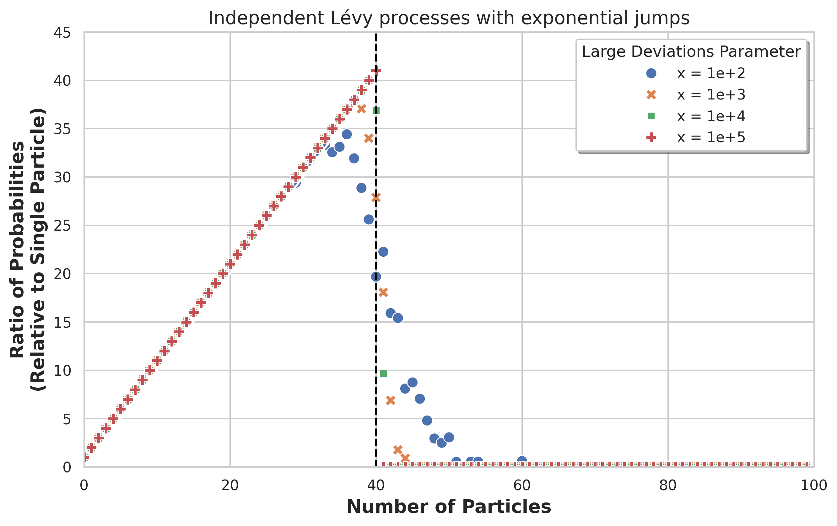
For the considered process, \(\psi(\lambda)= -\lambda + \frac{1}{2}\lambda^{2}- \frac{3\lambda}{\lambda + 1}+ \frac{2\lambda}{4 - \lambda}, \;\; \lambda < 4\) and its positive root turns out to be \(\lambda^* = 2\). Moreover, \(\psi'(2) = 8/3\) which gives, for \(B\) taken as \(B(x) = 15\cdot x\), an optimal number \(N^* = 40\) of particles.

For simulation purposes, as in the discrete-time case, we use the exponential martingale associated to \(\lambda^*\) and the measure \(\PP^{\lambda^*}\), as defined in Section 4. Specifically, the parameters of the process were chosen in such a way that under the measure \(\PP^{\lambda^*}\), the process is again Lévy with exponential jumps. Moreover the time intensities and the jump rates are permuted: under the measure \(\PP^{\lambda^*}\) the parameters of the Lévy measure are \(r^*=4\), \(\alpha^* = 2\), \(s^* = 1\) and \(\beta^* = 3\).

3.3 Exploration with restart for random walks and Lévy processes↩︎

Our Strategy II consists of restarting a random walk or a Lévy process as those studied in Theorems 1 and 2 upon leaving \((0,x)\) with a given probability measure \(\nu_x\) supported in the interval \((0,x)\). Our first result in this direction, stated in Theorem 3, gives asymptotic performance guarantees of restart strategies under mild assumptions on the restart measures \(\nu_x\), as \(x\to+\infty\).

In the next section we will specialize to a particularly interesting family of measures: quasi-stationary measures, for which better estimates are obtained (in particular matching bounds up to multiplicative constants). We remark that for the QSD case we rely exclusively on quasi-stationarity and related properties but not on Theorem 3.

This notion is sometimes called first-order stochastic domination and is equivalent to \(\nu_1(x,+\infty)\) being less or equal than \(\nu_2(x,+\infty)\) for every \(x\in\RR\).

The next theorem provides estimates on the time it takes for the restarted process to reach the desired region (here an interval \([x,+\infty)\) for large \(x\)) under mild assumptions on the restart measures \((\nu_x)_{x\geq 1}\), for which we assume without loss of genearality that \(x\geq 1\).

A typical trajectory of the restarted process is a concatenation of independent cycles, each of which consists of a trajectory \(\{y_0 + Z(t): 0\leq t \leq \tau\}\) for some \(y_0\in (0,x)\) sampled according to \(\nu_x\) and \(\tau \mathrel{\vcenter{:}}= \inf\{t>0: y_0 + Z(t) \notin (0,x)\}\). An intuition behind the result is that adding \(\nu_x\) as an initial distribution boosts the performance by a factor \(\int_0^x\exp(\lambda^* y)\nu_x(dy)\) for each cycle. Since the cycles’ duration is stochastically bounded we expect to observe an asymptotically-linear amount of cycles within time \(B(x)\). However a matching upper bound remains elusive for this general context.

As a final example for this section we take a simple extension of Example 4 that shows that Theorem 3 covers cases beyond weak convergence:

3.4 Restart with quasi-stationary measures.↩︎

We now specialize to an important family of restarting measures for which we can obtain sharper asymptotic results than those provided by Theorem 3.

Throughout this section we assume that \(\nu_x\) is the quasi-stationary distribution (QSD) of the process restricted to the interval \((0,x)\). We begin with a few brief preliminaries on quasi-stationary distributions, and refer the reader to the monograph [14] for a comprehensive treatment of the subject.

The study of QSD for a given Markov process is a subtle matter, in general they may not exist and when they do they may not be unique.

For the particular case of a one-dimensional Lévy process with absorbing set \(A = \RR\setminus (0,a)\) for some \(a>0\), by [15] there is a unique QSD, provided the distribution of the process without absorption at any time \(t>0\) is absolutely continuous with respect to Lebesgue in \(\RR\), which is satisfied since we are assuming a strictly positive diffusion coefficient. When there is a unique QSD, it is obtained as the Yaglom limit \[\lim_{t\to+\infty} \PP_y(Z(t)\in \cdot\;|\;t < \tau(A));\] which is independent of the starting position \(y\in \cS\setminus A\).

Existence of a Yaglom limit for a Lévy process when the absorbing set is \((-\infty,0]\) was proved in [16]¹, extending the case without jumps of [17].

To the best of our knowledge, there is no analogous existence-and-uniqueness result specific to discrete-time random walks conditioned on non-absorption on bounded intervals. If the law of the increments of a random walk is absolutely continuous with respect to the Lebesgue measure, then one may consider the associated compound Poisson process (CPP) with rate \(1\), thereby obtaining a Lévy process with an absolutely continuous law for every time larger than its first jump. By checking that for large \(t\) the probability of not having jumped is negligible for the CPP even when conditioned on non-absorption by time \(t\), one obtains the same Yaglom limit as the conditioned CPP and in particular existence and uniqueness given by [15]. This can be carried out using the asymptotics on passage times from [18]. These asymptotics for conditioned processes are used in the proof of Lemma 4 of Section 6. Yaglom limits for random walks with absorption at \((-\infty,0]\) were studied in [19], and under Cramér condition in [20].

We may now state our main theorem for restarted processes:

The theorem states that the application of a restarting mechanism with quasi-stationary distributions improves performance by a factor comparable with the time budget times an exponential moment of the respective measure. In the Brownian motion case, this improvement factor is exponential in the complexity of the task. Indeed, while \(\PP(\tau(x)\leq B(x))\) is of order \(e^{-2\mu x}\), with the restarting mechanism we get order \(B(x)e^{-\mu x}\). For a general Lévy process, exponential moments of its quasi-stationary measures are not easy to estimate. We conjecture that they grow as \(\exp\left[(\lambda^*-\lambda_0) x\right]\), as \(x\to+\infty\), where \(\lambda_0\) is the positive solution of \(\psi'(\lambda) = 0\). Note that this is exactly the case for the linear Brownian motion. For spectrally negative Lévy processes, namely when \(\Pi(0,+\infty) = 0\), the conjecture might be proved with the use of a Girsanov transformation of the process into a zero-drift one (thus providing the conjectured exponential factor) and applying the results of [21]. We do not pursue this further here, it is left as a direction of further study.

3.4.1 Simulations for restarted Lévy processes↩︎

We now present numerical experiments for restarted processes. As a case study, we consider the Lévy process with exponential jumps introduced in Subsection 3.2.1, equipped with a restart mechanism activated upon exiting the interval \((0,50)\subset\mathbb{R}\).

For the process without restart, recall that the Cramér exponent is \(\lambda^* = 2\). Consequently, when the process is started from the origin, the probability of ever reaching the upper barrier at \(50\) is of order \(\exp(-100)\). As restart measure, we consider an exponential distribution with mean \(10\), truncated to \((0,50)\), namely \[\nu_{50}(dx) = \frac{0.1\,e^{-0.1x}}{1-e^{-5}}\,\mathbf{1}_{(0,50)}(x)\,dx.\] Its exponential moment of order \(\lambda^*\) satisfies \[\int_0^{50} e^{2x}\,\nu_{50}(dx) \;\approx\; 9.6\times 10^{39}.\] Multiplying by \(\mathbb{P}_0(\tau(50)<+\infty)\) yields \[\mathbb{P}_0(\tau(50)<+\infty) \int_0^{50} e^{2x}\,\nu_{50}(dx) \;\approx\; 3.6\times 10^{-4}.\]

Although this estimate is only heuristic, in view of Theorem 3 it suggests that the probability of exceeding the level \(x=50\) within a finite time horizon \(B(50)\) under this restart strategy is no longer negligible. This behavior is confirmed numerically in Figure 3, which reports empirical mean estimates based on \(100\) independent replications for each time budget, together with \(95\%\) confidence intervals. The figure illustrates how the restart mechanism makes the exceedance of the upper barrier observable on moderate time scales, with confidence intervals (CI) indicating the associated variability.

We emphasize that the simulations reported in this section do not rely on importance sampling or on any other variance–reduction technique. The numerical results therefore illustrate that introducing a restart mechanism alone can already lead to a significant improvement in the simulation of rare events. In particular, restarting makes it possible to turn probabilities that are extremely small for the original process into quantities that can be reliably estimated within reasonable computational time.

4 Proof of Theorems 1 and 2↩︎

We begin the section by introducing some preliminaries on exponential martingales, first for random walks and then for Lévy process, which will be used in the proofs. They are standard techniques for the study of large deviations events for light tails, as is our case.

4.1 Preliminaries↩︎

By assumption 2 , the family of exponential martingales indexed by \(\lambda \in \Lambda_+\) may be defined as: \[M^{\lambda}_t \coloneq \exp\left( \lambda Z(t) - t\psi(\lambda) \right), \quad t \in \mathbb{N}.\] Indeed, \(M^{\lambda}\) is a martingale for every \(\lambda \in \Lambda_+\), which acts as a density for a new probability measure on the same probability space. Specifically, we define the measure \(\mathbb{P}^{\lambda}\) as \[\label{eq:exp95change95of95measure} \mathbb{P}^{\lambda}(A) \coloneq \mathbb{E}\left[M_{\tau}^{\lambda} \mathbf{1}(A)\right],\tag{12}\] where \(A\) depends on \(\{Z(t)\}_{t \leq \tau}\), and \(\tau\) is any almost-surely finite stopping time. The measure \(\mathbb{P}^{\lambda^*}\), associated with \(\lambda^*\) in equation 4 , will be of particular importance.

We also observe that the density of \(\mathbb{P}|_{\mathcal{F}_{\tau}}\) with respect to \(\mathbb{P}^{\lambda}|_{\mathcal{F}_{\tau}}\) is given by \((M^{\lambda}_{\tau})^{-1}\).

Exponential martingales are particularly useful for computing probabilities of rare events, as these events may become more frequent under \(\mathbb{P}^{\lambda}\) if \(\lambda\) is appropriately chosen. Under the measure \(\mathbb{P}^{\lambda}\), the increments \(X_j\), \(j \geq 1\), are i.i.d. (making \(Z\) a random walk), with mean and variance given by: \[\mu(\lambda) \mathrel{\vcenter{:}}= \mathbb{E}_{\lambda}[X_1] = \psi'(\lambda) \quad \text{ and } \quad \sigma(\lambda) \mathrel{\vcenter{:}}= \mathbb{E}_{\lambda}\left[ |X_1 - \mu(\lambda)|^2 \right] = \psi''(\lambda).\] The threshold in Theorem 1 can thus be interpreted in terms of the measure \(\mathbb{P}^{\lambda^*}\): the random time \(\tau(x)\) is \(\PP^{\lambda^*}\)-almost surely finite (since \(\psi'(\lambda^*)>0\)) with mean \(x \psi'(\lambda^*)^{-1}\), asymptotically as \(x \to +\infty\).

For Lévy process we have analogous definitions: under Cramér’s condition the family \(\{M^{\lambda}_t\}_{0\leq t\leq \lambda_{\max}}\) of exponential martingales is defined as \[M^{\lambda}_t \mathrel{\vcenter{:}}= \exp(\lambda Z(t) - t\psi(\lambda)),\] and the corresponding family of measures is given by \[\frac{d\PP^{\lambda}}{d\PP}\Bigg|_{\cF_t} = M^{\lambda}_t.\]

Under any of the measures \(\PP^{\lambda}\), \(Z\) is again a Lévy process with Lévy exponent \[\label{eq:change95measure95LP95exponent} \psi^{(\lambda)}(r) = \psi(\lambda + r)- \psi(\lambda),\tag{13}\] with mean and variance again given by: \[\mu(\lambda) \mathrel{\vcenter{:}}= \mathbb{E}_{\lambda}[X_1] = \psi'(\lambda) \quad \text{ and } \quad \sigma(\lambda) \mathrel{\vcenter{:}}= \mathbb{E}_{\lambda}\left[ |X_1 - \mu(\lambda)|^2 \right] = \psi''(\lambda).\]

From 13 it is straightforward to check that the corresponding characteristic triplet is given by: \[\label{eq:change95measure95LP} \mu_{\lambda} = -\mu+\lambda \sigma^2+\int_{-1}^1 y(e^{\lambda y }-1)\Pi(dy),\;\;\sigma_{\lambda}^2 = \sigma^2,\;\;\Pi^{\lambda}(dy) = e^{\lambda y}\Pi(dy).\tag{14}\]

The measure \(\PP^{\lambda^*}\) provides an intuition to Theorem 2 as in the random walk case: the law of the process conditioned to reach the high barrier is distributed as \(\PP^{\lambda^*}\). We do not prove this exact result here but lies at the core of the references cited for our proof [22], [23].

4.2 Proofs↩︎

Theorems 1 and 2 will follow from the following asymptotics of the passage times of random walks and Lévy processes with the assumptions on their exponential moments stated in Subsection 3.1.

The following proposition unifies [24] for the case of random walks and [23] for Lévy processes:

Some remarks are now in order:

5 Proof of Theorem 3↩︎

For the proof of Theorem 3 we will need the following auxiliary lemmas:

Assuming these we may now give the main result for restarted processes.

5.1 Proofs of auxiliary lemmas:↩︎

6 Proof of Theorem 4↩︎

In this section \(Z\) denotes either a random walk on discrete time or a Lévy process, satisfying Cramér’s condition, and we will consider as restarting measures the family of quasi-stationary distributions \((\nu_x)_{x\geq1}\). The proof of Theorem 4 relies on some auxiliary results.

Once the sequence of measures admits a weak limit, Remark [remark:weak95convergence95and95domination] provides a route to apply Theorem 3, thereby yielding the lower bound in Theorem 4. We adopt, however, a different approach that relies more heavily on properties associated with quasi-stationarity.

If we assume the lemmas above we may prove the main result as follows:

Before proving the lemmas we compute the quasi-stationary distribution, its exponential moment of order \(\lambda^*\) and the absorption rate for a linear Brownian motion explicitly.

6.1 Proofs of auxiliary lemmas:↩︎

We now turn to the proof of the auxiliary lemmas.

7 Conclusion↩︎

This paper investigates various exploration strategies under time constraints in environments with unknown stochastic dynamics focusing on their impact on performance as measured by the time required to reach a set of rare states.

We aim for this work to be a foundational step towards developing a more qualitative theory of exploration, specifically by incorporating the time needed to observe meaningful signals for the first time. For example in Reinforcement Learning environments with sparse rewards, exploration of the state space or action-state space is widely recognized as a critical bottleneck to efficiency. By addressing this crucial aspect, we seek to contribute to more efficient and effective exploration strategies in such contexts and beyond.

In this work, we focused on space-invariant one-dimensional dynamics, which provide highly interpretable results and for which we can provide explicit performance guarantees. Building on this understanding, future work will consider more general Markovian dynamics, providing a more comprehensive and realistic framework for exploring challenging environments. A natural extension of this work is to higher-dimensional settings. While explicit hitting-time estimates of the kind used here are generally unavailable in that regime, the “too-many-particles" phenomenon and the core conclusions of our main results are expected to carry over to considerably more general settings.

Appendix I: M/M/1↩︎

In this section we investigate the interplay between the probability of exploration, under the time regime of interest, and the efficiency of the associated estimation procedure. In particular, we show that the variance of the natural Monte Carlo estimator mirrors the typical exploration time.

Consider an \(\mathrm{M/M/1}\) queue on the truncated state space \(\{0,1,\dots,n\}\) with load parameter \(\rho<1\), and assume that \(X(0)=0\) almost surely. The chain is ergodic, and its invariant measure is geometrically decaying: for any \(k\in\mathbb{N}\) with \(k\le n\), the stationary weight is proportional to \(\rho^k\). By the Ergodic Theorem, the stationary measure \(\pi\) satisfies \[\pi(k) = \lim_{t\to\infty} \frac{1}{t}\int_0^t \mathbf{1}\bigl(X(s)=k\bigr)\,ds .\] A Monte Carlo estimator for \(\pi(k)\), based on a time horizon \(B(k)\), is therefore \[\widehat{\pi}(k) = \frac{1}{B(k)}\int_0^{B(k)} \mathbf{1}\bigl(X(s)=k\bigr)\,ds .\]

We focus on restrictive time budgets and assume that the estimation of \(\pi(k)\) for large \(k\) is performed with a linear-in-\(k\) horizon, \[B(k)\asymp k, \qquad k\to\infty .\] In such a regime, the process is expected to spend exceedingly little time in state \(k\): indeed, the expected hitting time of \(k\) grows exponentially fast in \(k\). As we show next, this scarcity of observations is the principal obstruction to reliable estimation, and it directly governs the variance of the Monte Carlo estimator.

Fix \(c>0\) and introduce the surrogate estimator \[\xi(k) \mathrel{\vcenter{:}}= c\, \mathbf{1}\bigl(\tau(k)< B(k)\bigr),\] where \(\tau(k)\) denotes the hitting time of state \(k\). Then, by noting that \(\widehat{\pi}(k) + \xi(k)\) is almost surely bounded by \(1+c\), and that \(\bigl| \widehat{\pi}(k) - \xi(k) \bigr|\bfone(\tau(k)>B(k)) = 0\), one obtains:

\[\begin{gather} \bigl|\operatorname{Var}\,\widehat{\pi}(k) - \operatorname{Var}\,\xi(k)\bigr| = \Bigl|\mathbb{E}_0\bigl[(\widehat{\pi}(k)-\xi(k))(\widehat{\pi}(k)+\xi(k))\bigr] \\ - \mathbb{E}_0(\widehat{\pi}(k)-\xi(k))\, \mathbb{E}_0(\widehat{\pi}(k)+\xi(k))\Bigr| \\ \leq 2(1+c)\cdot \mathbb{E}_0|\widehat{\pi}(k) -\xi(k)| \\ \leq \mathrm{const}\cdot \mathbb{P}_0\!\bigl(\tau(k)\le B(k)\bigr), \end{gather}\] for some constant independent of \(k\), thus showing that the variance is essentially governed by the rare-event probability of reaching \(k\) within the available time budget.

Appendix II: The Fleming-Viot particle system and FVRL↩︎

The approach found in [3] for defining a restarted mechanism is based on the paradigm of Fleming-Viot (FV) particle system, introduced by [4]. In this framework, a population of particles (which can represent different simulations in parallel) evolves over time, exploring the state space in parallel. When a particle falls into a less promising region \(A\), it is “restarted" by being replaced with a copy of another, more promising particle. This ensures that resources are concentrated on exploring the most fruitful areas of the state space. The FV strategy is particularly effective in scenarios where certain regions of the state space are more likely to yield valuable rewards, as it dynamically reallocates exploration effort towards these regions, thereby increasing the overall efficiency of the exploration process.

Note that various papers [29]–[31] have shown that FV empirical measures converge as the number of particles tend to infinity to the conditioned evolution of the process, i.e., \[m_t^N(A) \to P(X_t \in A | T \ge t ), N \to \infty,\] where \(T\) is the hitting time of \(A\). On the other hand \(P(X_t \in A | T \ge t ) \to \nu(A)\), as \(t \to \infty\) where \(\nu\) is the (a for countable state space) QSD associated with the process absorbed in \(A\). This is the motivation for restarting according to the QSD in our work.

Appendix III: An example in RL: the control of blocking in a \(M/M/1/K\)↩︎

This example has been considered in [3] and generalized to multidimensional settings (several coupled queues). It serves here as a canonical illustration of Reinforcement Learning in environments with sparse and rare rewards where the exploration is the main bottleneck. We summarize the model and the FVRL strategy introduced in [3] as a motivation for our theoretical results. Consider an \(M/M/1/K\) queue with fixed buffer capacity \(K\), arrival rate \(\lambda\), service rate \(\mu\), and load \(\rho = \lambda/\mu < 1\). The state space is \(\cS = \{0,1,\dots,K\}\), representing queue occupancy. The control action \(a \in \{0,1\}\) determines whether to accept (\(a=1\)) or block (\(a=0\)) arriving jobs. The reward function is structured to penalize both the under-utilisation of resource and large blocking probabilities: \[r(x,a) = \begin{cases} 0 & \text{if } a = 1 \\ B(1 + b^{x - x_{\text{ref}}}) & \text{if } a = 0 \end{cases}\] with \(B > 0\), \(b > 1\), and reference state \(x_{\text{ref}}\). This structure induces threshold-optimal policies (blocking all the incoming traffic after a given threshold). For threshold policies parameterized by \(\theta\), we define the policy-dependent blocking threshold \(K_\theta = \lfloor \theta \rfloor + 1\), representing the state at which the policy \(\pi_\theta\) begins rejecting incoming jobs. To ensure that the blocking threshold never exceeds the physical buffer, the policy parameter is restricted to the compact domain \(\Theta = [0, K-1]\), so that \(K_\theta \leq K\) is guaranteed at all times. Under the average reward criterion and using a policy gradient strategy, one aims at minimizing: \[J^{\pi_\theta} = \sum_{x \in \cS} p^{\pi_\theta}(x) \sum_{a} \pi_\theta(a|x) Q_{\theta}(x,a),\] where \(\theta \in \Theta\) is the parametrisation of the policy. The policy gradient theorem yields: \[\nabla_\theta J^{\pi_\theta} = \sum_{x \in \cS} p^{\pi_\theta}(x) \sum_{a} Q_{\theta}(x,a) \nabla_\theta \pi_\theta(a|x)\] For threshold policies parameterized by \(\theta \in \Theta\), this simplifies to: \[\label{grad:est} \nabla_\theta J^{\pi_\theta} \propto p^{\pi_\theta}(\mathbf{K_\theta}-1) \left[ Q_{\theta}(\mathbf{K_\theta}-1,1) - Q_{\theta}(\mathbf{K_\theta}-1,0) \right]\tag{34}\] where \(K_\theta = \lfloor \theta \rfloor + 1\) is the learned blocking threshold, and the gradient is concentrated at state \(K_\theta - 1 = \lfloor \theta \rfloor\), the last state before the policy blocks under the current parameterization \(\theta \in \Theta\).

The Gradient Estimation Problem:↩︎

Given this framework, the RL strategy will be efficient if the gradient estimates can be informative. We discuss here only the estimate of the stationary probability \(p^{\pi_\theta}(\mathbf{K_\theta}-1)\). The stationary distribution for state \(\mathbf{K_\theta}\), under the threshold policy \(\pi_\theta\), is given by the \(M/M/1/K_\theta\) formula: \[p^{\pi_\theta}(\mathbf{K_\theta}) = \frac{(1-\rho)\rho^{\mathbf{K_\theta}}}{1-\rho^{\mathbf{K_\theta}+1}}.\] For typical parameters (\(\rho = 0.7\), \(K_\theta = 40\)), \(p^{\pi_\theta}(\mathbf{K_\theta}) \sim \mathcal{O}(10^{-7})\). Since \(p^{\pi_\theta}(\mathbf{K_\theta}-1) \sim p^{\pi_\theta}(\mathbf{K_\theta})/\rho\), both are exponentially small.

Consequently:

• Vanilla Monte Carlo estimators of \(p^{\pi_\theta}(\mathbf{K_\theta}-1)\) exhibit prohibitive variance (in terms of multiplicative errors),

• Much more importantly, the policy gradient in 34 becomes numerically zero under finite sampling. Hence, the learning signal vanishes, preventing convergence to an optimal \(\theta\).

7.1 Parallel sampling↩︎

In order to compare our results with those of [3], we present a set of simulations for parallel \(\mathrm{M/M/1}\) queues under different time regimes. The hyperparameters used in Figure 4 are: total queue capacity \(K=40\), initial condition \(J=12\), arrival rate \(\lambda=0.7\), and service rate \(\mu=1\). In this numerical illustration, \(K_\theta = K = 40\), so that \(p^{\pi_\theta}(K)\) is the exponentially rare quantity identified in the Gradient Estimation subsection above.

Following [3], we estimate the stationary probability via a renewal-type decomposition based on successive returns to \(J\). More precisely, we estimate (i) the expected return time to state \(J\), which in our setting is of order \(10^2\), and independently (ii) the probability of hitting \(K\) starting from \(J\). For the latter we report estimators under time horizons \(B(K)\) of magnitudes \(10^5\), \(10^6\), and \(10^7\), and we compare them with the true stationary value \(\mathbf{p^{\pi_\theta}(K)}\) shown in Figure 4.

To ensure a fair comparison with the experiment of [3], we remark that the total number of events observed in our simulations—counting both arrivals and departures—is one to two orders of magnitude larger than theirs. Indeed, across our time regimes we record approximately \(1.7\times 10^r\) events for \(r=5,6,7\), which exceeds the event counts reported in [3]. This discrepancy is natural: correlations in the Fleming–Viot particle system substantially facilitate the exploration of the rare state \(K\).

In summary, and as expected, the estimation accuracy with independent particles lies between that of naive Monte Carlo (which rarely reaches \(K\) even for time of order \(10^6\)) and that of the Fleming–Viot particle system.

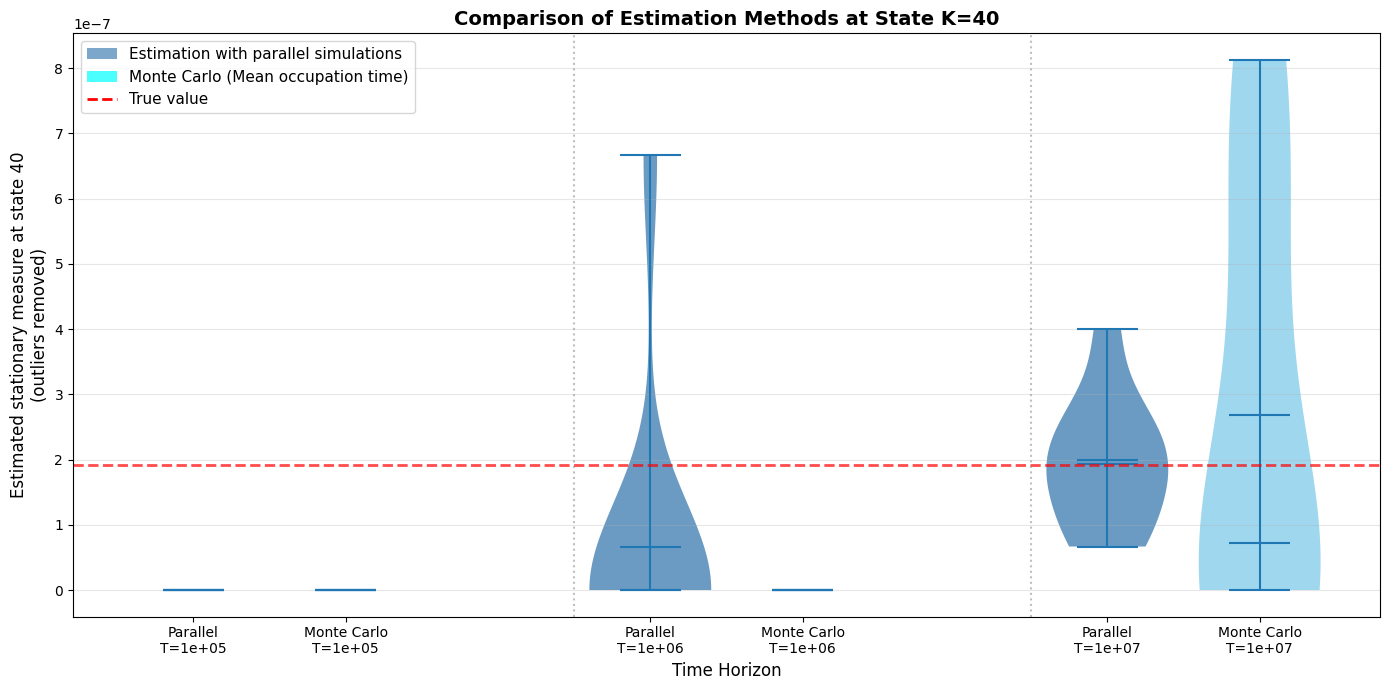
7.2 Fleming-Viot Solution↩︎

The FVRL method addresses this by introducing an absorption set, where prior knowledge is used on the fact that no rewards is granted in \(\cal A= \{0,1,\dots,J-1\}\) with \(J < K\). The Fleming-Viot particle system consists of \(N\) particles \((\xi_t^{\nu}(i))_{i=1}^N\) evolving in \(\cal A^c\), with resetting mechanism: particles hitting \(\cal A\) jump to positions of randomly selected surviving particles. This particle system approximately estimates the quasi-stationary distribution: \[\nu_Q^{\pi}(x) = \lim_{t\to\infty} \PP^{\partial\cal A^c}(X_t^{\pi} = x | T_{\mathcal{K}} > t)\] where \(T_{\mathcal{K}}\) is the hitting time of \(\cal A\). The FV-RL algorithm leverages this to construct gradient estimators: \[\widehat{\nabla_\theta v^{\pi_\theta}} = \sum_{x \in \AA^c} \hat{p}^{\pi_\theta}(x) \sum_{a} \hat{Q}_{\theta}(x,a) \nabla_\theta \pi_\theta(a|x)\] where \(\hat{p}^{\pi_\theta}\) is estimated via the FV particle system.

For \(K = 40\), \(\rho = 0.7\):

• Vanilla MC estimates \(p^{\pi}(K) \approx 0\) even with \(10^6\) samples

• FV provides accurate estimates with \(N \sim 10^3\) particles

• FVRL converges to \(K^*\) while MC-based policy gradient fails completely

The method effectively trades the rare event probability \(p^{\pi}(K)\) for the substantially larger quasi-stationary probability \(\nu_Q^{\pi}(K)\), overcoming the exponential sample complexity of vanilla approaches. We do not compare here with our results of the estimates constructed in [3] are more complex than the idealized situation described in Section 3.4 which can however serve as a rule of thumb for practitioners.

References↩︎

---

1. The processes we consider fall in their class A category with parameter \(\alpha=2\).↩︎

2. The notation \(\asymp\) was introduced in Remark [rmk:asymp95notation].↩︎

3. see [26] for the analogous result for discrete-time random walks↩︎