Moderate-length lifted quantum Tanner codes
February 27, 2025
Abstract
We introduce new families of quantum Tanner codes, a class of quantum codes that first appeared in the work of Leverrier and Zémor [1]. These codes are built from two classical Tanner codes, for which the underlying graphs are extracted from coverings of 2D geometrical complexes, and the local linear codes are tensor-products of cyclic or double-circulant linear codes. The advantage of code lifting is that, for any lift of odd index \(t\) of an \([[n,k,d]]\)-code, we can adapt the study of the transfer homomorphism arising in cellular homology to describe symmetries of its logical operators and to establish that its dimension is lower bounded by \(k\), and its distance is upper bounded by \(t\cdot d\). Moreover, when the dimension of the lifted code is equal to \(k\), its distance is lower bounded by \(d\). These parameter bounds also apply to the previous methods of code lifting [2]. Finally, We present several explicit families, and identify instances of moderate length quantum codes which are degenerate, have low check weight, and whose distance surpasses the square root of the code length. Among them, we report the existence of a \([[96,2,12]]\)-code whose distance growth saturates our bound, and for which half of the checks are of weight 8 and the other half of weight 4.
1 Introduction↩︎
Quantum error correcting codes are believed to be unavoidable constituents of quantum computing architectures. Among them, quantum low-density parity-check (LDPC) codes are the leading candidates for physical implementations, because their low connectivity translates into a limitation of the error propagation between the hardware constituents. Significant progress has been made recently in the construction of good quantum LDPC codes [1], [3], [4], i.e. codes families with constant rate and relative distance in the asymptotic limit. These families can constitute a valuable source of inspiration to devise new types of codes of moderate length, following the effort in the design of near term implementable codes [5]–[7].
In 2022, Leverrier and Zémor [1] generalized the Sipser-Spielman version [8] of classical Tanner codes [9] to devise a new family of asymptotically good CSS codes, which they call quantum Tanner codes. The methodology of [1] relies on two components: a family of geometric complexes and a set of short linear codes. They instantiated it by considering a class of 2D square complexes known as left-right Cvayley complexes, first used in the coding context in [10]. Given one of these complexes, its face-vertex incidence structure generates two graphs, each used to define a classical Tanner code. The local structure of the complex allows for classical tensor-product codes to be used as local codes, which is key to ensure commutation between stabilizers of the quantum code. Although this CSS construction is state-of-the-art in the asymptotic regime, short-length examples based on the same ideas have not yet been developed.
This article introduces new families of quantum Tanner codes, inspired by the Leverrier-Zémor construction [1], [11]. The main novelty of our approach is that we start by defining a quantum Tanner code on a square complex, which is not necessarily a left-right Cayley complex or a constant-degree graph as in [12]. Recall that exploring beyond constant degree Tanner graphs has been key to devise capacity-approaching classical LDPC codes [13]. We then use our construction to build larger quantum Tanner codes based on the idea of code lifting.
Our approach to lift is also largely inspired by the method of [3] to lift classical Tanner codes. Here, instead of using only a graph and a local code, we work with a 2-dimensional square complex over which two classical Tanner codes can be defined, forming an input CSS code. A covering of the square complex then allows us to simultaneously define lifts of these two classical Tanner codes. The maximum weight of the rows and columns of the lifted check matrices remains equal to that of the input code, making it well-suited for LDPC constructions. A peculiarity of our lifting method is that the size of the overlapping support of an \(X\)- and a \(Z\)-check can be reduced under lifting. This shows that this method is different from the one defined in [2] for which the size of the overlap is conserved under lifting.
The drawback of our method is that lifting a CSS code does not always yield a valid CSS code. To ensure that lifting yields a valid CSS code, the symmetries of the local codes must be compatible with the structure of the underlying 2D complex. The advantage is that for lifts of odd indices, we can adapt the study of the transfer homomorphism, arising in cellular homology [14], to establish a lower bound on the dimension of lifted codes and to describe the structure of their logical operators. Namely, a lifted \([[\tilde{n}, \tilde{k},\tilde{d}]]\)-code of odd index \(t\) of a \([[n,k,d]]\)-code, has \(\tilde{n}=tn\), \(\tilde{k}\geq k\) and \(\tilde{d}\leq td\). Moreover, when \(\tilde{k}=k\), it follows that \(\tilde{d}\geq d\). The technics and parameter bounds developed here also apply to the code lifting method of [2], based on coverings of the Tanner cone-complex.
We illustrate the lifting of quantum Tanner codes through explicit examples. In [2], new code constructions were introduced using certain 2D geometric complexes, namely square subdivisions of presentation complexes of finitely presented groups; the CSS codes were built by interpreting the vertices, in the subdivision of these complexes, as parity checks and qubits. Here, following [1], we adopt a different perspective and interpret the faces as qubits. The novelty of our method is to first construct short-length quantum Tanner codes on these subdivided complexes by fixing a specific configuration of the local codes. We then obtain the lifted Tanner code by generating coverings of these square complexes and lift the local code configuration to the covering spaces. In certain cases, the effect of the local code is to suppress the short codewords, causing the support of minimal codewords to spread out across the complex. In this way, we are able to construct LDPC codes whose distance squared exceeds the blocklength.
It has proven challenging to determine analytically the parameters of our lifted Tanner codes. We therefore follow a numerical approach. For selected input quantum Tanner codes, we generate all possible lifts of index 1 to 30, producing codes of length
less than 800 qubits. An upper bound for the distance is computed using GAP and the package QDistRnd [6]. We report only the codes with the highest
parameters and leave a more rigorous analysis for future work.
This article is organized as follows. In Section 2, we set the notation for graphs, square-complexes and covering maps. We also review classical Tanner codes and our preferred method for lifting them.
In Section 3, we present a method to lift a quantum Tanner code. The idea is a generalization of the lift of a classical Tanner code, where the central object is a covering of a square complex rather than a graph. We also extend the study of the transfer homomorphism from cellular homology to characterize the structure of any lifted codes of odd index.
Lastly, in Section 4, we introduce new explicit constructions of quantum Tanner codes. We then perform an exhaustive numerical search for lifted codes and report specific instances with the highest distances.
2 Preliminaries↩︎
2.1 Graphs and square-complexes↩︎
In this work, crucial components of the linear and quantum code constructions are graphs and square complexes. We therefore set some notations and state elementary facts about these objects, which will be used throughout this article.
2.1.0.1 Graphs.
We denote by \(\mathcal{G}:=(V,E)\) an undirected graph with set of vertices \(V\) and edges \(E\). An edge between two vertices \(u\) and \(v\) is an unordered pair \(\{u,v\}=\{v,u\}\). In this work, graphs have no self-loops, i.e., edges of the form \(\{u,u\}\), unless otherwise stated, but they can have multi-edges. A directed edge associated to \(\{u,v\}\in E\) is an edge for which the order matters, written \(e=[u,v]\) for an edge with initial vertex \(u\) and terminal vertex \(v\). The inverse of an edge is defined as \([u,v]^{-1}:=[v,u]\). We denote by \(E^*\) the set of oriented edges. Its cardinality is twice that of \(E\). A path of length \(t\) in the graph is a sequence of directed edges \(e_1\cdot e_2\dots e_t\) such that the terminal vertex of \(e_i\) is the initial vertex of \(e_{i+1}\), for \(i<t\). A path is closed if the terminal vertex of \(e_t\) is the initial vertex of \(e_1\). The
edge-neighborhood of a vertex \(v\), denoted \(E(v)\), is the set of edges connected to \(v\), and its cardinality is the degree of \(v\). A \(t\)-cycle in \(\mathcal{G}\) is a connected subgraph constituted of \(t\) vertices (of degree 2 in the
subgraph) and \(t\) edges, forming a single cycle in \(\mathcal{G}\).
2.1.0.2 Square complexes.
A square complex is defined as a graph with a set of preferred subgraphs which are 4-cycles. We denote it \(\mathcal{S}:=(V,E,F)\), where \((V,E)\) is the underlying graph, also called its 1-skeleton, and \(F\) is a set of 4-cycles. Notice that a square complex with an empty set of faces is also a graph. We say that \(\mathcal{S}\) is a bipartite square complex if \((V,E)\) is a bipartite graph. A face \(f\in F\) can be described by its corresponding \(4\)-cycle, or by a closed path, such as \(\alpha_f=[v_1,v_2].[v_2,v_3].[v_3,v_4].[v_4,v_1]\). The face-neighborhood of a vertex \(v\) is the set of faces to which it is incident, and is denoted \(F(v)\). Moreover, we say that two faces are adjacent in \(\mathcal{S}\) if they share a common edge.
2.1.0.3 Topological realization.
the topological realization of a square complex is a topological space divided into 2D and 1D subspaces. For us, it is most convenient to view the topological realization of a square complex as a regular 2D cell complex [14] (or CW complex). These are topological spaces obtained by successively gluing cells, with gluing maps being homeomorphisms1. More precisely, in the topological realization of a square complex, for each combinatorial face, we glue an actual face, which is homeomorphic to a two-dimensional disk \(D^2\), along the path formed by a 4-cycle. The resulting complex is then endowed with the topology of a CW complex.
Here, when we construct graphs and square complexes, we identify them with their topological realization. This is because we consider their fundamental group, defined in the next section, and perform geometrical operations on them. It is important to note that every abstract 2D complex defines a topological one and vice versa.
2.2 Fundamental group↩︎
For considerations related to covering spaces in Section 2.3, it will be important to introduce the fundamental group, a central object in algebraic topology [14], [15].
2.2.0.1 Definition.
We first recall that given a topological space \(K\) the fundamental group \(\pi_1(K,v)\) is the group of homotopy classes of loops based at \(v\), with group operation given by loop concatenation. For any other choice of basepoint \(v'\), the groups \(\pi_1(K,v)\) and \(\pi_1(K,v')\) are isomorphic. In what follows, we will often omit the choice of basepoint and simply write \(\pi_1(K)\). A space is called simply connected if its fundamental group is trivial.
2.2.0.2 Combinatorial approach for square-complexes.
As previously mentioned, a square complex can be viewed as a 2D cell complex via its topological realization. In that setting, the fundamental group is defined as above. Moreover, there is an equivalent description of the fundamental group that solely relies on the combinatorial data of the square complex. This description, which we now review, is convenient for computations, and it is often used to determine presentations of the fundamental group.
Given a closed path \(e_1\cdot e_2\dots e_n\) an elementary reduction consists of either removing two consecutive edges \(e_i\) and \(e_{i+1}\) if \(e_{i+1} = e_i^{-1}\), or removing four consecutive edges if the corresponding sequence forms a face in the square complex \(K\). The equivalence relation generated by such reductions is called homotopy; it is compatible with concatenation of closed path, where the concatenation of two paths \(\alpha:=e_1\cdot e_2\dots e_t\) and \(\alpha':=e'_1\cdot e'_2\dots e'_{t'}\), such that the terminal vertex of \(e_t\) is the initial vertex of \(e_1'\), is the path \(\alpha\cdot\alpha':=e_1\cdot e_2\dots e_t\cdot e'_1\cdot e'_2\dots e'_{t'}\). The fundamental group \(\pi_1(\mathcal{S},v)\) is then isomorphic to the set of homotopy classes of closed paths based at \(v\), with concatenation as the group operation. It can be shown that \(\pi_1(\mathcal{S},v) \cong \pi_1(\mathcal{S},v')\) for any two vertices \(v, v'\), if its 1-skeleton \(\mathcal{S}^1:=(V,E)\) is a connected graph, and thus we often write \(\pi_1(\mathcal{S})\).
If a square complex \((V,E,F)\) has no faces, i.e. it is just the connected graph \((V,E)\), then the fundamental group of its topological realization is a free group of rank \(|E| - |V| + 1\). For a general 2D complex having a graph \(\mathcal{G}\) for 1-skeleton, the fundamental group is given by the quotient \(\pi_1(\mathcal{G})/N\), where \(N\) is the normal closure of the subgroup generated by elements corresponding to 4-cycles.
2.3 Covering maps↩︎
We now review some results about covering maps from [14]–[16]. While some of them apply to topological spaces in general, we will only consider them in the context of graphs and square-complexes of finite degrees with a single connected component.
2.3.0.1 Graph coverings.
Let \(\mathcal{G}\) be a graph, that we identify with its topological realization. A map between graphs \(p:\mathcal{G}' \to \mathcal{G}\) is a covering if and only if it is continuous, it maps interior of edges homeomorphically onto interior of edges, and every vertex of \(\mathcal{G}'\) has a neighborhood on which the restriction of \(p\) is a homeomorphism.
For graphs, we may prefer a combinatorial definition of covering. Let us now see the graphs above simply as sets of vertices and edges with no self-loops. Then, a graph covering is a surjective map \(p:\mathcal{G}' \to \mathcal{G}\) that maps edges to edges and vertices to vertices and such that the restriction of \(p\) to the edge neighborhood of every vertex is a bijection. It follows that a vertex \(v\) in \(\mathcal{G}'\) and its image \(p(v)\) have the same degree. The cardinality of the inverse image of any vertex or edge is a constant called the index of the covering.
From [17], such a map can be given a topological realization, which is a continuous function from a topological realization of \(\mathcal{G}'\) to a topological realization of \(\mathcal{G}\) whose restriction to the interior of any edge of \(\mathcal{G}'\) is a homeomorphism and is consistent with \(p\). A map \(p\) between graphs is a combinatorial covering if and only if a topological realization of \(p\) is a covering in the usual sense.
2.3.0.2 Permutation voltage.
We now summarize a construction for graph coverings that can generate all possible finite coverings, as shown in [16]. Let \(r>0\) be an integer and \(S_r\) be the symmetric group on the set \([r]:=\{0,\dots,r-1\}\). Given a graph \(\mathcal{G}=(V,E)\), we first assign a permutation \(\pi_e\in S_r\) to each oriented edge \(e\in E^*\), with the constraint that \(\pi_{e^{-1}}=\pi_{e}^{-1}\). This step is called a permutation voltage assignment. We construct a graph \(\tilde{\mathcal{G}}\), called a lifted graph, with set of vertices in bijection with \(V\times [r]\) and set of edges in bijection with \(E\times [r]\), where an element \(c\) of \(\tilde{\mathcal{G}}\), vertex or edge, is written \((c,i)\) for \(i\in [r]\). An edge \((e,i)\) in the graph \(\tilde{\mathcal{G}}\), where \(e=[u,v]\), connects \((u,i)\) and \((v,\pi_e (i ))\).
As proved in [16], given a lifted graph constructed as above, it is possible to define a covering map \(p:\tilde{\mathcal{G}}\rightarrow \mathcal{G}\) acting on an element \((c,i)\), vertex or edge, by \(p((c,i))=c\). Conversely, for any \(r\)-sheeted graph covering \(p:\mathcal{G}'\rightarrow \mathcal{G}\), there exists a permutation voltage assignment of \(\mathcal{G}\) in \(S_r\), such that the associated lifted graph is isomorphic to \(\mathcal{G}'\). We indeed verify that all the conditions are verified, and in particular a vertex \((v,i)\) and its projection \(v\) have the same degree. Moreover, an edge \(\tilde{e}=[\tilde{u},\tilde{v}]\) projects onto an edge \(e=[p(\tilde{u}),p(\tilde{v})]\).
2.3.0.3 Square complex coverings.
Given a square complex \(\mathcal{S}=(V,E,F)\), an index-\(r\) covering \(\tilde{\mathcal{S}}\) is a graph covering \(p:\tilde{\mathcal{G}}\rightarrow \mathcal{G}\) which does not break the faces. That is, if \(\alpha\) is a 4-cycle in \(\mathcal{G}\) describing a face of \(F\), then \(p^{-1}(\alpha)\) is a set of \(r\) disjoint 4-cycles. The set of faces in the covering is in bijection with \(F\times [r]\), and given a face \(f\in F\) described by the path \[e_1.e_2.e_3.e_4=[v_1,v_2].[v_2,v_3].[v_3,v_4].[v_4,v_1],\] then for all \(i\in [r]\), the face labeled \((f,i)\) in \(\tilde{\mathcal{S}}\) can be described by the following 4-cycle:
Figure 1:  .
.
in other words, for any \(4\)-cycle described by a closed path \(e_1.e_2.e_3.e_4\) corresponding to an element of \(F\), the permutation \(\pi_{e_4}\circ\pi_{e_3}\circ\pi_{e_2}\circ \pi_{e_1}\) is the identity. We can then define an index-\(r\) covering map \(p:\tilde{\mathcal{S}}\to \mathcal{S}\) acting on an element \((c,i)\) (vertex, edge or face) by \(p((c,i))=c\), and therefore \(p\) maps faces to faces. The inverse image of any vertex, edge or face is a set of \(r\) vertices, edges or faces.
2.3.0.4 Deck transformations.
We now consider a square-complex \(\mathcal{S}\), possibly with an empty set of faces, i.e. a graph. Given a covering \(p:\tilde{\mathcal{S}}\to \mathcal{S}\), a deck transformation2 is an automorphism \(\psi:\tilde{\mathcal{S}}\rightarrow \tilde{\mathcal{S}}\) such that \(p\circ \psi=p\). The set of deck transformations, endowed with the operation of composition of maps, forms a group denoted \(\operatorname{deck}(p)\). It is called the group of deck transformations and acts on the left on \(\tilde{\mathcal{S}}\). A Galois covering is a covering enjoying a left, free and transitive action of \(\operatorname{deck}(p)\) on the fiber. For any Galois covering, \(p:\tilde{\mathcal{S}}\rightarrow \mathcal{S}\), it can be shown that \(\operatorname{deck}(p)\setminus \tilde{\mathcal{S}}\cong \mathcal{S}\).
In the rest of this section, by a covering \(p:\tilde{\mathcal{S}}\to \mathcal{S}\) we always mean a finite connected covering, i.e. one whose index is finite and for which \(\tilde{\mathcal{S}}\) is also a connected complex. The following crucial results of this section apply in this context.
2.3.0.5 Classification of coverings.
The theory of connected covering maps over a complex depends on the structure of its fundamental group in the following way. For every index \(r\) subgroup \(H\) of the fundamental group \(\pi_1(\mathcal{S})\) there exists an index \(r\) covering \(p:\mathcal{S}_H\to \mathcal{S}\), mapping the basepoint \(\tilde{v}\) of \(\mathcal{S}_H\) to \(v\), and inducing an injective homomorphism \(p_\#:\pi_1(\mathcal{S}_H,\tilde{v})\to \pi_1(\mathcal{S},v)\), such that \(p_\#\pi_1(\mathcal{S}_H , \tilde{v}) = H\). A covering \(p:\mathcal{S}_H\to \mathcal{S}\) is called Galois or normal when \(H\) is a normal subgroup of \(\pi_1(\mathcal{S},v)\). All the coverings that we will study in Section 4 are of this form. It can be shown that, for such a covering map, we have the isomorphism \(\operatorname{deck}(p)\cong\pi_1(\mathcal{S},v)/H\). The most important result on coverings is the classification theorem known as the Galois correspondence, which we state in our restricted setting of finite index coverings of complexes with finitely many cells.3
Theorem 1 (Galois correspondence). For all \(r\in \mathbb{N}\), there is a bijection between the set of basepoint-preserving isomorphism classes of index-\(r\) connected covering spaces of a complex \(\mathcal{S}\) and the set of index-\(r\) subgroups of \(\pi_1 (\mathcal{S})\). Given such a covering \(p:\tilde{\mathcal{S}}\to \mathcal{S}\), it is obtained by associating the subgroup \(H=p_\#\pi_1 (\tilde{\mathcal{S}} )\) to the covering space \(\tilde{\mathcal{S}}\). The index of the associated covering is equal to the index \([\pi_1(\mathcal{S}):H]\).
This theorem motivates our exhaustive searches of all possible Galois coverings in Section 4.
2.4 Tanner codes and their lifts↩︎
In this section, we recall some definitions and set up notations related to linear codes. The central components of our quantum codes are classical Tanner codes. We review their construction and a method to lift them into larger codes.
2.4.0.1 Linear codes.
We denote the parameters of a binary linear code \(C\subseteq \mathbb{F}_2^n\) as \([n,k,d]\), where \(n\) its the length, \(k\) its dimension and \(d\) its distance, defined as \(d=\min\limits_{c\in C\setminus \{0\} }|c|\). If \(k=0\), our convention is to set \(d=\infty\). In what follows, a linear code will be defined by the image of a linear map \(g:\mathbb{F}_2^k\to \mathbb{F}_2^n\), or the kernel of a linear map, \(h:\mathbb{F}_2^n\to \mathbb{F}_2^m\), respectively represented in a preferred basis \(B\) by a generator matrix \(G:=\operatorname{Mat}_B (g)\), and a parity-check matrix \(H:=\operatorname{Mat}_B (h)\). Given \(x\in \mathbb{F}_2^n\), the vector \(s=Hx\) is called the \(syndrome\) of \(x\). The generator matrix of \(C\) is the parity-check matrix of its dual \(C^\perp=\{x\in \mathbb{F}_2^n\: :\: \forall c\in C, \langle x,c\rangle=0\}\). A code is called self-dual when \(C^\perp=C.\)
2.4.0.2 Classical Tanner codes.
The central components of our quantum codes are classical Tanner codes, introduced in [9], and made popular by Sipser and Spielman [8]. We first review their construction, and then we describe a natural method to lift them into larger Tanner codes.
Let \(\mathcal{G}=(V,E)\) be a graph on \(|E|=n\) edges. In the following, \(\mathbb{F}_2E := \bigoplus_{e\in E}\mathbb{F}_2 e\) denotes the space of formal linear combinations of elements of the set \(E\), playing the role of basis vectors. Given a vertex, \(v\), the space \(\mathbb{F}_2E(v)\), is the restriction of \(\mathbb{F}_2E\) to the edge neighborhood of \(v\). We define a set of binary local codes \(C_V := (C_v )_{ v\in V}\) on the vertices of \(\mathcal{G}\), where an element indexed by \(v\in V\) is a code defined on the edge neighborhood of \(v\), i.e. \(C_v \subseteq \mathbb{F}_2E(v)\). For a vector \(c\in \mathbb{F}_2 E\), we denote by \(c|_{E(v)}\) its restriction to the edge-neighborhood of \(v\).
Definition 1 (Classical Tanner code). Let \(\mathcal{G}=(V,E)\) be a graph and \(C_V=(C_v )_{ v\in V}\) be a set of binary local codes. We define the Tanner code associated to \(\mathcal{G}\) and \(C_V\) as \[T(\mathcal{G},C_V) := \{ c\in \mathbb{F}_2E : c|_{E(v)}\in C_v\text{ for all }v\in V\}.\]
2.4.0.3 Parity-check matrix.
A Tanner code can also be defined as the kernel of a parity-check matrix. Suppose that \(C_v\) is the kernel of a linear map \(h_v:\mathbb{F}_2E(v)\to \mathbb{F}_2^{r_v}\) and let \(i_v: \mathbb{F}_2^{r_v}\to \bigoplus_{u\in V} \mathbb{F}_2^{r_u}\) be the canonical linear embedding map. The Tanner code \(C=T(\mathcal{G},C_V)\) is the kernel of the map \(h :\mathbb{F}_2 E\xrightarrow[]{} \bigoplus_{u\in V} \mathbb{F}_2^{r_u}\) defined on an edge \(e\) between vertices \(v\) and \(w\) by \[\label{equation:tanner32code32map} h (e)= i_v\circ h_v (e) + i_w\circ h_w (e),\tag{1}\] and extended by linearity over \(\mathbb{F}_2 E\). All vector spaces being given with a preferred basis, \(h_v\) can be represented by a matrix \(H_v\) of size \(r_v\times |E(v)|\), and \(h\) by a matrix \(H\) of size \(r\times n\), where \(r=\sum_{v\in V} r_v\). Denoting \(w\), \(w_v\), the maximum row-weight of \(H\) and \(H_v\), respectively, and \(q,q_v\) their column-weight, we have \[w=\max\limits_{v\in V }w_v, \quad \quad q\leq\max \limits_{ \{v,w\}\in E} q_v+q_w .\] This justifies why this technique is particularly suitable for constructing LDPC codes.
2.5 Lift of Tanner codes↩︎
Linear code lifting is an operation of major interest to produce interesting LDPC codes [18] in a wide range of block lengths. Recall that lifting amounts to constructing a covering of the Tanner graph representation of the code. In this work, we focus on lifts of Tanner codes. In that case, out of the many possible lifts, there exists a preferred choice that we simply refer to as the lift of a Tanner code, as we will not use other types of lifts. From now on, we consider a graph \(\mathcal{G}\) that has no self-loops. Given a graph covering \(p:\tilde{\mathcal{G}}\to \mathcal{G}\), where \(\tilde{\mathcal{G}}=(\tilde{V},\tilde{E})\), the linear extension \(p_\#\) of \(p\) on the set of edges induces an isomorphism4 \[\mathbb{F}_2\tilde{E}(\tilde{v})\overset{p_\#}{\cong} \mathbb{F}_2 E(v),\]for any \(\tilde{v}\in p^{-1}(v)\). By definition, \(p_\#\) sends basis vectors to basis vectors, i.e. edges to edges.
Definition 2 (Lift of Tanner code). Let \(C=T(\mathcal{G},C_V)\) and \(p:\tilde{\mathcal{G}}\to \mathcal{G}\) be a graph covering, with \(\tilde{\mathcal{G}}=(\tilde{V}, \tilde{E})\). For each vertex \(\tilde{v}\in \tilde{V}\), we associate the code \(C_{\tilde{v}}\subseteq \mathbb{F}_2E(\tilde{v})\), such that \(C_{\tilde{v}} \overset{p_\#}{\cong} C_{p(\tilde{v})}\). The lifted Tanner code associated to \(p\) is the code \(\tilde{C}=T(\tilde{\mathcal{G}},C_{\tilde{V}})\), where \(C_{ \tilde{V}}= (C_{\tilde{v}})_{ \tilde{v}\in \tilde{V}}\). In other words, \[T(\tilde{\mathcal{G}},C_{\tilde{V}})=\{c\in \mathbb{F}_2 \tilde{E} \: :\: p_\#(c|_{\tilde{E}(\tilde{v})})\in C_{p(\tilde{v})}, \text{for all }\tilde{v}\in \tilde{V}\} .\]
2.5.0.1 Parity-check matrix.
Suppose that for each \(v\in V\), \(C_v\) is the kernel of a map \(h_v\) represented by a matrix \(H_v\), as described after Equation 1 . This induces a parity-check matrix \(H\) of size \(r\times n\) for the Tanner code \(C\). In this context, by lifting we always mean that for any \(\tilde{v}\in p^{-1}(v)\), we define the code \(C_{\tilde{v}}\) as the kernel of a map \(h_{\tilde{v}}\) represented by the matrix \(H_{\tilde{v}}=H_v\). In this way, fixing a matrix representation \(H\) induces a matrix representation \(\tilde{H}\), the parity-check matrix of \(\tilde{C}\), up to permutation of the rows. For a covering of index \(t\), this matrix has size \(tr\times tn\). Denoting \(\tilde{w}\), \(\tilde{q}\) as the maximum row and column-weight of \(\tilde{H}\), we have \[\label{Equation:32lift32conserve32degree} \tilde{q}=q, \quad \tilde{w}=w.\tag{2}\] This can also be deduced from the fact that the lift of a Tanner code is an example of lift of a classical code associated to a specific type of covering over the Tanner graph associated to \(H\).
2.6 Local codes↩︎
Throughout this work, for an integer \(\ell\geq 1\), we denote \([\ell] := \{ 0,\dots ,\ell-1\}\).
2.6.0.1 Classical tensor-product codes.
The classical local codes that will constitute our Tanner codes are built as duals of tensor-product codes. The tensor-product of two linear codes, \(C\subseteq \mathbb{F}_2^{\ell_C}\) and \(D\subseteq \mathbb{F}_2^{\ell_D}\), is the linear code denoted \[\Pi=C\otimes D\subseteq \mathbb{F}_2^{\ell_C}\otimes \mathbb{F}_2^{ \ell_D}.\] The canonical bases of \(\mathbb{F}_2^{\ell_C}\) and \(\mathbb{F}_2^{\ell_D}\) are indexed by the elements of \([\ell_C]\) and \([\ell_D]\),
respectively. These bases naturally induce the canonical product basis for \(\mathbb{F}_2^{\ell_C}\otimes \mathbb{F}_2^{ \ell_D}\), whose elements are indexed by \([\ell_C]\times[\ell_D]\).
In this basis, the codewords of the product code can be seen as the \(\ell_C\times\ell_D\) matrices all of whose rows and columns are, respectively, codewords of \(C\) and \(D\). We may describe a parity-check matrix of \(\Pi\) as follows. Let \(H_C\) and \(H_D\) be parity-check matrices for \(C\) and \(D\), respectively. Then the codewords of \(\Pi\) are the vectors \(x\in \mathbb{F}_2^{\ell_C}\otimes \mathbb{F}_2^{
\ell_D}\) satisfying both \[(H_C\otimes I) x=0\quad \text{and}\quad (I\otimes H_D)x=0.\] The first condition ensures that every row vector of \(x\), seen as a \(\ell_C\times\ell_D\) matrix, is in \(C\), and the second that every column vector is in \(D\). A parity-check matrix \(H\) of
\(\Pi\) is hence given by vertically joining these two sets of equations: \[H=\begin{bmatrix} H_C\otimes I\\ I\otimes H_D
\end{bmatrix}.\] It follows that the dual of the tensor-product is \[\label{equation32dual32of32tensor32product32code}
\Pi^\perp=C^\perp\otimes \mathbb{F}_2^{\ell_D}+ \mathbb{F}_2^{\ell_C}\otimes D^\perp.\tag{3}\] Indeed, the rows of a parity-check matrix generate the dual code, and the first and second sets of equations of \(H\) generate the first and second summands of Equation 3 , respectively.
In the tensor codes considered later, one of the factors is a repetition code of length \(2\) and the other one is either a cyclic or a double-circulant code. We therefore recall some essential facts about these two types
of codes, taken from [19].
2.6.0.2 Cyclic codes.
A binary cyclic code \({C} \subseteq \mathbb{F}_2^\ell\) is a code that is stable under the action of the automorphism \(\rho :\mathbb{F}_2^\ell \to \mathbb{F}_2^\ell, (c_0, \ldots, c_{\ell-1})\mapsto(c_{\ell-1},c_0,\ldots, c_{\ell-2})\).
A practical way to define a cyclic code is to identify \(\mathbb{F}_2^\ell\) and the polynomial ring \(R_\ell := \mathbb{F}_2[X]/{(X^\ell-1)}\), using the \(\mathbb{F}_2\)-linear isomorphism \[\varphi: R_\ell \longrightarrow \mathbb{F}_2^\ell,\quad g_0 + g_1 X + \cdots + g_{\ell-1}X^{\ell-1} \longmapsto (g_0, \ldots,g_{\ell-1}).\] In \(R_\ell\), the transformation corresponding to the rotation \(\rho\) is multiplication by \(X\). A code \(C\subseteq R_\ell\) is cyclic if it is stable under this operation, and by linearity it is an ideal of \(R_\ell\). These ideals are in one-to-one correspondence with the divisors of \(X^\ell-1\). Given \(g \in \mathbb{F}_2 [X]\) such that \(g ~|~ X^\ell-1\), the code \(\mathscr{C}_\ell (g)\) is defined as the code equal to the ideal generated by \(g\), and \(g\) is referred to as the generating polynomial of the code. It is well-known that \(\mathscr{C}_\ell (g)\) has dimension \(\ell-\deg (g)\).
The dual of a cyclic code is cyclic, and its generating polynomial can be obtained as follows. Given a polynomial \(h\in R_\ell\), let \(\bar{h} := X^{\deg h}h(1/X)\) denote the reciprocal polynomial of \(h\). Over \(\mathbb{F}_2\), \(X^\ell - 1\) is equal to its reciprocal polynomial so, if \(h~|~X^\ell-1\), then \(\bar{h}~|~X^\ell-1\). Letting \(h\) be the polynomial such that \(gh = X^\ell-1\), also called the check-polynomial, we have \(\mathscr{C}_\ell (g)^{\bot} = \mathscr{C}_\ell (\bar h)\).
Given any polynomial \(f\in R_\ell\), we define \(\mathbb{G}(f)\) as the circulant matrix whose first row is \(\varphi(f)\). Note that \(G=\mathbb{G}(g)\) is a square generator matrix of the code. The row-weight of \(G\) is hence directly given by the weight of \(g\), i.e. its number of non-zero coefficients.
2.6.0.3 Double-circulant codes.
The second type of linear codes considered in the tensor-product are double-circulant codes. They form a subclass of quasi-cyclic codes, built from any polynomial \(f\in R_\ell\). The double-circulant code \(\mathscr{D}_{2\ell}(f)\subseteq \mathbb{F}_2^{2\ell}\) is defined as the image of the generator matrix \[G= \left[\begin{array}{c|c} \mathbb{G}(1) & \mathbb{G}(f) \end{array}\right],\] where \(\mathbb{G}(1)\) corresponds to the \(\ell\times\ell\) identity matrix. In Section 4.3, the ambient space \(\mathbb{F}_2^{2\ell}\) of a double-circulant code \(\mathscr{D}_{2\ell}(f)\) is always understood to be given with the canonical basis indexed by the columns of the generating matrix in the above form. It is important to note that the code generated by \(G\) is invariant under simultaneous cyclic permutation within the left and right blocks. That is, the code is stable under the automorphism \[\sigma:\begin{cases} \hfill \mathbb{F}_2^{2\ell}\hfill &\longrightarrow \qquad \mathbb{F}_2^{2\ell} \\ (c_0, c_1,\dots,c_{2\ell-1})&\mapsto (c_{\ell-1},c_0, \ldots, c_{\ell-2},c_{2\ell-1},c_\ell, \ldots, c_{2\ell-2}). \end{cases}\] Hence, \(\mathbb{Z}_\ell\) is a subgroup of the automorphism group \(\operatorname{Aut}(\mathscr{D}_{2\ell}(f))\). The dual of \(\mathscr{D}_{2\ell}(f)\) is generated by the matrix \[H=\left[\begin{array}{c|c} \mathbb{G}(\bar f)&\mathbb{G}(1) \end{array}\right],\] and is also invariant under simultaneous cyclic permutations within the left and right blocks.
3 Quantum Tanner codes and their lifts↩︎
3.1 Quantum Tanner codes↩︎
3.1.0.1 Quantum CSS codes.
CSS codes are instances of stabilizer quantum error correcting codes, which first appeared in the seminal work of Calderbank, Shor and Steane [20]–[22]. Let \(C_X\) and \(C_Z\) be two linear codes with parity-check matrices \(H_X\) and \(H_Z\), such that \(C_X^\perp\subseteq C_Z\), referred to as the orthogonality condition. The CSS code \(\text{CSS}(C_X,C_Z)\) is the subspace \[\operatorname{Span}\left \{\sum_{z\in C_Z^\perp }\ket{x+z}\text{ } \: :\:\text{ } x\in C_X \right \}\] of \((\mathbb{C}^2)^{\otimes n}\). Its parameters, denoted \([[n,k,d]]\), are its length \(n\), dimension \(k = \dim(C_X / C_Z^\perp)\) and distance \(d\). The latter is defined as \(d := \min(d_X, d_Z)\), with \[d_X=\min\limits_{c\in C_Z\setminus C_X^\perp}|c|, \quad d_Z=\min\limits_{c\in C_X\setminus C_Z^\perp}|c|.\] The maximum row weight and column weight in the parity check matrix \(H_X\), respectively \(H_Z\), are denoted \(w_X,q_X\), respectively \(w_Z, q_Z\). We denote \(W:=\operatorname{max}(w_X,q_X,w_Z,q_Z)\). A family of codes is called Low Density Parity Check (LDPC) if \(W\) is upper bounded by a constant. If \(k=0\), our convention is to set \(d=\infty\).
The only CSS codes that we consider in this article are quantum Tanner codes, a class of codes introduced by Leverrier and Zémor [1], in which \(C_X,C_Z\) is a pair of classical Tanner codes.
3.1.0.2 Square complexes and diagonal graphs.
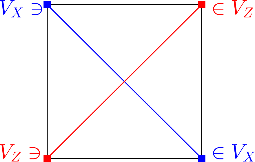
A practical way to build two Tanner codes \(C_X\) and \(C_Z\) satisfying the orthogonality condition is to generate them simultaneously by considering two specific graphs embedded in a square complex. Let \(\mathcal{S} := (V,E,F)\) be a bipartite square complex and denote the partition \(V=V_X \sqcup V_Z\). As remarked in [1], if we restrict the vertex set to \(V_X\), each square face is now incident to only two vertices located at opposite corners. The set of squares \(F\) can now be seen as a set of edges on \(V_X\), and therefore it defines a graph that we denote by \(\mathcal{G}_X^\Box=(V_X,F)\) and call the diagonal graph on \(V_X\). Similarly, restricting the vertex set to those of \(V_Z\), we obtain the diagonal graph \(\mathcal{G}_Z^\Box=(V_Z,F)\). These graphs, illustrated in Figure 2, can then be treated as the graph components of two classical Tanner codes whose set of bits are identified with \(F\), and as so we can identify the ambient space of these codes as \(\mathbb{F}_2F\).
3.1.0.3 Local product structure.
The idea behind quantum Tanner codes is to use a square complex endowed with a specific structure.
Definition 3. Let \(\mathcal{S}=(V,E,F)\) be a square complex. We say that \(\mathcal{S}\) has a local product structure if, for every vertex \(v\in V\), there exist sets \(A_v\) and \(B_v\), and bijections \((\phi_v)_{v\in V}\) such that \(\phi_v:F(v)\to A_v\times B_v\), where \(F(v)\) is the face neighborhood of \(v\). Moreover, for any pair of adjacent vertices \(v\) and \(v'\), either \(A_v=A_{v'}\) or \(B_v=B_{v'}\). In the former case, there are elements \(b\in B_v\) and \(b'\in B_{v'}\) such that \(\phi^{-1}_v(A_v\times \{b\})=\phi^{-1}_{v'}(A_{v'}\times \{b'\})\). In the latter case there are elements \(a\in A_v\) and \(a'\in A_{v'}\) such that \(\phi^{-1}_v(\{a\}\times B_v)=\phi^{-1}_{v'}(\{a'\}\times B_{v'})\).
We say that a local product structure is strict if \(\phi^{-1}_v(\{a\}\times \{b\})=\phi^{-1}_{v'}(\{a\}\times \{b'\})\) for every \(a\in A_v\) in the former case, and if \(\phi^{-1}_v(\{a\}\times \{b\})=\phi^{-1}_{v'}(\{a'\}\times \{b\})\) for every \(b\in B_v\) in the latter case.
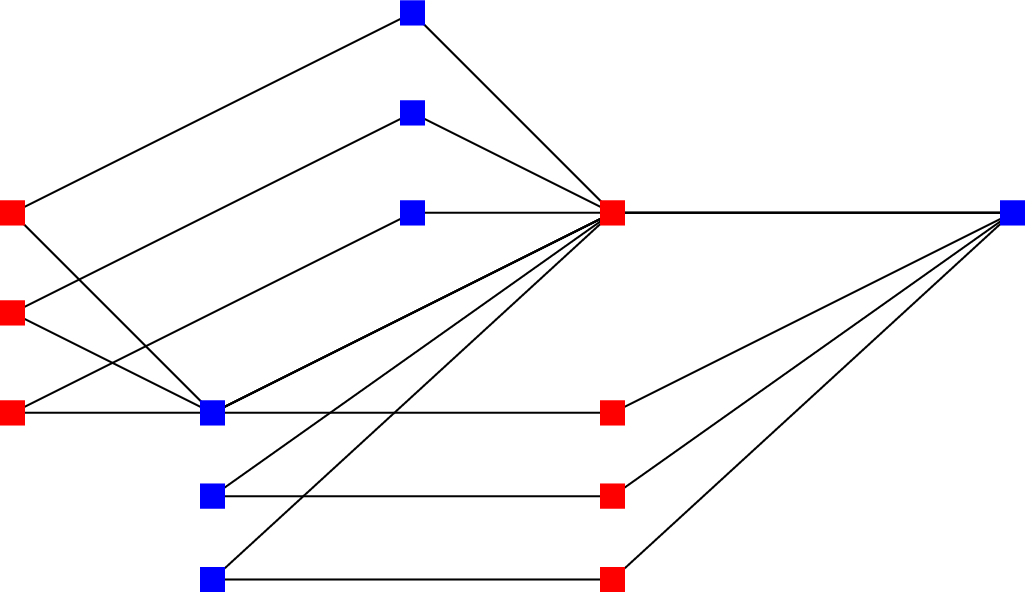
The local product structure of a square complex is illustrated in Figure 3. The left-right Cayley complex of [10] can be given a strict local product structure. This was exploited in the quantum Tanner code construction of [1].
3.1.0.4 Choice of local codes.
To fully define \(C_X\) and \(C_Z\), we must coherently assign local codes \(C_{V_X}\) and \(C_{V_Z}\) to the vertices of the graphs \(\mathcal{G}_X^\Box\) and \(\mathcal{G}_Z^\Box\), respectively. When \(\mathcal{S}\) has a local product structure, it is natural to choose the local codes to be classical tensor product codes. Here, for simplicity we detail the case where the local product structure is strict. However, we will later go beyond this constraint, which will require our local codes to have certain symmetries.
Given two adjacent vertices \(v_x\) and \(v_z\) in such a square complex, let us assume that \(\phi_{v_x}:F(v_x)\to [\ell]\times[\ell']\) and \(\phi_{v_z}:F(v_z)\to [\ell]\times [\ell'']\), where \(\ell, \ell'\) and \(\ell''\) are all positive integers. We can see these bijections as indexings of face neighborhoods. Suppose also that the intersection of their neighborhoods is of the form \([\ell]\times \{i\}\) according to the indexing of \(F(v_x)\), and \([\ell]\times \{j\}\) for that of \(F(v_z)\). We can extend \(\phi_{v_x}\) by linearity into a map \(\phi_{v_x}: \mathbb{F}_2F(v_x)\to \mathbb{F}_2^{\ell}\otimes \mathbb{F}_2^{ \ell'}\) mapping faces to canonical basis vectors. We consider local codewords of the product code \(C\otimes C' \subseteq \mathbb{F}_2^{\ell}\otimes \mathbb{F}_2^{ \ell'}\), where \(C\) is a code of length \(\ell\) and \(C'\) is a code of length \(\ell'\). This code can be represented as the set of binary \(\ell\times\ell'\) matrices, all of whose rows and columns are elements of \(C\) and \(C'\), respectively. By extending \(\phi_{v_z}\) by linearity into a map \(\phi_{v_z}: \mathbb{F}_2F(v_z)\to \mathbb{F}_2^{\ell}\otimes \mathbb{F}_2^{ \ell''}\), we can also consider local codewords of the product code \(C^\perp\otimes C''^\perp\) defined in \(F(v_z)\), where \(C\) is as previously, and \(C''\) is a code of length \(\ell''\). Codewords can be similarly represented in a \(\ell\times \ell''\) matrix. When the local indexing of the faces is strict, the intersection \(F(v_x)\cap F(v_z)\) is mapped by \(\phi_{v_x}\) and \(\phi_{v_z}\) to a column in each of the two matrices. This column supports codewords of \(C\) in the first, and codewords of \(C^\perp\) in the second, as shown in Figure 4. Since we chose a code and its dual, they overlap on an even number of positions in \(\tilde{F}:=F(v_x)\cap F(v_z)\). That is, given \(c_x\in C\otimes C'\) and \(c_z\in C^\perp\otimes C''^\perp\), we denote \(\tilde{c}_x\) and \(\tilde{c}_z\) the restrictions of \(\phi^{-1}_{v_x}(c_x)\) and \(\phi^{-1}_{v_z}(c_z)\) to \(\mathbb{F}_2 \tilde{F}\), respectively. By our choice of local codes, we automatically have \(\langle \tilde{c}_x,\tilde{c}_z\rangle=0\). We can hence define the local codewords \(\phi^{-1}_{v_x}(c_x)\) and \(\phi^{-1}_{v_z}(c_z)\) as parity-check constraints associated with the code \(C_{v_x}\) and \(C_{v_z}\), respectively.

When making such a consistent choice of local product codes across the entire square complex, we obtain two Tanner codes \[C_X=T(\mathcal{G}_X^\Box, C_{V_X} ), \quad C_Z=T(\mathcal{G}_Z^\Box, C_{V_Z}),\] such that \(C_X^\perp\subseteq C_Z\). Such a pair of classical codes defines a quantum Tanner code denoted \(T(\mathcal{S}, C_{V_X}, C_{V_Z})\).
The procedure above is better carried out case by case, especially when the local product structure is not strict. In that case, the assignment of the local codes depends on the global structure of the square complex. We illustrate it on explicit examples in Section 4.
3.2 Lifting quantum Tanner codes↩︎
We now describe a lifting procedure for quantum Tanner codes which differs from that of [2]. Our approach is an extension of the method applied in [3] to design a family of Sipser-Spielman codes [8] with optimal parameters. Here, we use a covering of a bipartite square complex in order to create a covering for each of its two diagonal graphs.
Suppose that \(\operatorname{CSS}(C_X, C_Z)\) is a quantum Tanner code, built over a bipartite square complex \(\mathcal{S}=(V=V_X\sqcup V_Z,E,F)\), with \(C_X=T(\mathcal{G}_X^\Box, C_{V_X} )\) and \(C_Z=T(\mathcal{G}_Z^\Box, C_{V_Z})\). Given a covering map \(p:\tilde{\mathcal{S}} \to \mathcal{S}\), the 1-skeleton of \(\tilde{\mathcal{S}}=(\tilde{V},\tilde{E},\tilde{F})\) is also bipartite with bipartition \(\tilde{V}=\tilde{V}_X\sqcup \tilde{V}_Z\), where \(\tilde{V}_X=p^{-1}(V_X)\) and \(\tilde{V}_Z=p^{-1}(V_Z)\). We can hence consider the diagonal graphs \(\tilde{\mathcal{G}}_X^\Box=(\tilde{V}_X,\tilde{F})\) and \(\tilde{\mathcal{G}}_Z^\Box=(\tilde{V}_Z,\tilde{F})\).
Using the notation above, we have the following lemma.
Lemma 1. The covering map \(p\) induces two covering maps \(p_X: \tilde{\mathcal{G}}_X^\Box \to \mathcal{G}_X^\Box\) and \(p_Z:\tilde{\mathcal{G}}_Z^\Box \to \mathcal{G}_Z^\Box\).
Proof. Suppose that \(p:\tilde{\mathcal{S}}\rightarrow \mathcal{S}\) is an index-\(t\) covering defined by an assignment of permutations to all the oriented edges of \(\mathcal{S}\), i.e \(\pi_e\in S_t\) for \(t>0\) such that \(\pi_{e^{-1}}=\pi_{e}^{-1}\). It is essential to note that \(\tilde{V}_X=p^{-1}(V_X)\), \(\tilde{V}_Z=p^{-1}(V_Z)\), and \(\tilde{F} =p^{-1}(F)\), so that we have \(t\) vertices or faces in \(\tilde{\mathcal{G}}_X^\Box\) projected by \(p\) onto each vertex or face in \(\mathcal{G}_X^\Box\), and similarly for the diagonal graph on \(V_Z\). We now need to show that these cells are assembled into coverings of the diagonal graphs.
Given a face \(f\in F\) described by the closed path of oriented edges \(e_1.e_2.e_3.e_4=[v_1,v_2].[v_2,v_3].[v_3,v_4].[v_4,v_1]\), then for all \(i\in [r]\), the face labeled \((f,i)\) in \(\tilde{\mathcal{S}}\) can be defined by the 4-cycle as described in Section 2.3. Therefore, if \(e=[v_1,v_3]\) is an edge in \(\mathcal{G}_X^\Box\), then an edge \((e,i)\) in the covering \(\tilde{\mathcal{G}}_X^\Box\), projected onto \(e\) by \(p\), is given by \([(v_1,i), (v_3,\pi_{e_2}\circ \pi_{e_1}(i))]\). Let us assign the permutation \(\pi_{e_2}\circ \pi_{e_1}\in S_t\) to \(e\). We can similarly assign a composition of two permutations to each diagonal edge of \(\mathcal{G}_X^\Box\), according to the corresponding square in \(\mathcal{S}\). This defines a covering map \(p_X: \tilde{\mathcal{G}}_X^\Box \to \mathcal{G}_X^\Box\). A similar procedure on \(\tilde{\mathcal{G}}_Z^\Box\) defines a covering map \(p_Z:\tilde{\mathcal{G}}_Z^\Box \to \mathcal{G}_Z^\Box\). ◻
We now have all the elements to define the lift of a quantum Tanner code. Notice that we can define two lifted classical Tanner codes from our square complex covering. Let \(\tilde{C}_X=T(\tilde{\mathcal{G}}_X^\Box ,C_{\tilde{V}_X})\) be the lift of \(C_X=T(\mathcal{G}_X^\Box, C_{V_X} )\) associated to \(p_X\), and \(\tilde{C}_Z=T(\tilde{\mathcal{G}}_Z^\Box ,C_{\tilde{V}_Z})\) be the lift of \(C_Z=T(\mathcal{G}_Z^\Box, C_{V_Z})\) associated to \(p_Z\). The codes \(\tilde{C}_X\) and \(\tilde{C}_Z\) are subspaces of a common vector space \(\mathbb{F}_2^{t\cdot n}\), where \(t\) is the index of the cover, and they are candidates for defining a new CSS code. This is conditioned on the fact that \(\tilde{C}_X\) and \(\tilde{C}_Z\) must satisfy the orthogonality condition, namely \(\tilde{C}_X^\perp\subseteq \tilde{C}_Z\). If that condition is satisfied, we define the lifted quantum Tanner code associated to \(p\) as the code \(\operatorname{CSS}(\tilde{C}_X,\tilde{C}_Z)\).
This definition suggests that the lifted classical Tanner codes associated to \(p_X\) and \(p_Z\) do not necessarily satisfy the orthogonality condition. This depends on certain properties of the complex \(\mathcal{S}\), and on the choice of local codes. However, there are cases where they always do, as shown below.
Proposition 2. Let \(\operatorname{CSS}(C_X,C_Z)\) be a quantum Tanner code over a bipartite square complex \(\mathcal{S}\) for which the face neighborhood of every vertex has a simply connected closure5, when seen as a cell complex. Then, the lifting procedure above, applied to every finite covering space \(p:\tilde{\mathcal{S}}\to \mathcal{S}\), defines a valid CSS code.
Proof. The face neighborhood of every vertex having a simply connected closure, the support intersection between a check of \(\tilde{C}_X\) and one of \(\tilde{C}_Z\), associated to two incident vertices of \(\tilde{\mathcal{S}}\), is isomorphic to the support intersection of their projections in \(\mathcal{S}\) by the covering map. ◻
In Figure 5, we show an example of a vertex in a square complex whose face neighborhood has a closure that is not simply connected.

The condition of Proposition 2 is satisfied for a wide range of quantum Tanner codes, including those built from square complexes which are products of two graphs, or left-right Cayley complexes satisfying the total-no-conjugacy-class condition [10]. It was shown in [2], that the quadripartite version of the left-right Cayley-complex of [10] can be obtained as a covering of a Cartesian product of graphs. This can be used to show that the quantum Tanner code family defined in [1], [11] on such left-right Cayley-complex can be obtained by quantum Tanner code lifting, similarly to the approach of [2].
Hereafter, we define quantum Tanner code families beyond the restriction on \(\mathcal{S}\) stated in Proposition 2. It means that the number of qubits shared by a pair of \(X\)- and \(Z\)-checks in the base codes is
not necessarily preserved under lifting. In particular, this shows that the lifting technique presented here is not equivalent to that of [2], where lifting a code preserved the size of the overlap between any pairs of \(X\)- and \(Z\)-checks. In Section 4, we give explicit examples where this phenomenon occurs.
In the rest of this article, we focus on specific types of square complex coverings.
Lemma 2. Let \(\mathcal{S}\) be a connected square complex for which every edge is incident to at least two faces, and let \(p:\tilde{\mathcal{S}}\to \mathcal{S}\) be covering.
If \(p\) is connected, then \(p_X\) and \(p_Z\) are also connected coverings.
If \(p\) is a Galois covering with group of deck transformations \(\Gamma\), then \(p_X\) and \(p_Z\) are also Galois with group of deck transformations \(\Gamma\).
Proof.
If every edge in \(\mathcal{S}\) is incident to at least two faces, then its diagonal graphs are also connected. Indeed, if two faces are adjacent in \(\mathcal{S}\), then their induced edges in either of the two diagonal graphs must also be adjacent, and by repeating this argument for any two distant faces in \(\mathcal{S}\) shows that any two edges in the diagonal graphs are connected by a path. This local property is preserved under taking a covering, showing that the diagonal graphs of \(\tilde{\mathcal{S}}\) are also connected.
If \(p:\tilde{\mathcal{S}}\to \mathcal{S}\) is a Galois covering, the diagonal graphs in \(\tilde{\mathcal{S}}\) must be connected as a consequence of the first item. Moreover, \(\tilde{\mathcal{G}}_X^\Box\) inherits the free transitive action of the group \(\operatorname{deck}(p)\), since we can see \(\tilde{\mathcal{G}}_X^\Box\) as a subcomplex of \(\tilde{\mathcal{S}}\) and \(p_X\) as a restriction of \(p\) to this subcomplex. Therefore, \(p_X: \tilde{\mathcal{G}}_X^\Box\to \mathcal{G}_X^\Box\) is also a Galois covering with a group of deck transformations \(\operatorname{deck}(p)\), and similarly for \(p_Z\).
◻
In this work, we say that the lift of a CSS code is Galois if it is associated to a Galois covering.
An automorphism of a quantum code \(C=\operatorname{CSS}(C_X,C_Z)\) is defined as a permutation of the coordinates of the qubits which is equivalent to a permutation of the parity checks of both \(H_X\) and \(H_Z\). The set of automorphisms of \(C\) forms the group \(\operatorname{Aut}(C)\). In the case of a lifted quantum Tanner code \(\tilde{C}\), notice that the group of deck transformations of \(p:\tilde{\mathcal{S}}\to \mathcal{S}\) is a symmetry group of the Tanner graph of the quantum code. It is also a symmetry group of each of the Tanner graphs associated to \(\tilde{H}_X\) and \(\tilde{H}_Z\). Thus, given an element6 \(\gamma \in \operatorname{deck}(p)\), a vector \(c\in \mathbb{F}_2 \tilde{F}\) with syndrome \(\tilde{H}_Xc=s_X\) and \(\tilde{H}_Zc=s_Z\) , there exist two permutations \(\sigma_X\) and \(\sigma_Z\) of the syndrome coordinates such that \(\tilde{H}_X\gamma(c)=\sigma_X(s_X)\) and \(\tilde{H}_Z\gamma(c)=\sigma_Z(s_Z)\). Therefore, \(\operatorname{deck}(p)\) is a subgroup of \(\operatorname{Aut}(\tilde{C})\). We will use this feature in Section 3.3 to characterize the logical operators of certain lifted codes.
3.3 Parameter bounds from transfer homomorphism↩︎
For a lift defined from a Galois cover of odd index, we can use our information on the base code and leverage covering theory to lower bound the dimension of the lifted code and to characterize the structure of the logical operators. To this end, we use the language of chain complexes, and a specific chain map called the transfer homomorphism [14] usually arising in the context of cellular homology, or more generally in group theory. Although the discussion and parameters bounds presented here holds for code lifting in general, such as the method of [2], we focus on lifted classical and quantum Tanner codes. Our findings can be straightforwardly applied to the codes of Example 4, and show that logical operators are invariant under cyclic permutations. More formally, the aim of this section is to prove the following bounds on the parameters of a lifted code.
Proposition 3. Let \(\tilde{C}\) be a quantum Tanner code obtained by a Galois \(t\)-lift, with \(t\) odd, of a quantum Tanner code \(C\) with parameters \([[n,k,d]]\). Then, the parameters \([[\tilde{n},\tilde{k},\tilde{d}]]\) of \(\tilde{C}\) satisfy \(\tilde{n}=tn\), \(\tilde{k}\geq k\), and \(\tilde{d}\leq td\). Moreover, if \(\tilde{k}=k\), then \(\tilde{d}\geq d\).
Remark 4. The validity of Proposition 3 extends to the code lifting method of [2], as made clear from the technics, which does not depend on the structural specificities of quantum Tanner codes. In particular, the result just relies on the lifted quantum code \(\tilde{C}\) to be a chain complex of free modules over a group \(\Gamma\) of order \(t\).
3.3.0.1 Classical and quantum codes as chain complexes.
Recall that a classical code can be seen as the first homology group of the chain complex \(C_1\xrightarrow[]{h} C_0:=\mathbb{F}_2^n\xrightarrow[]{h} \mathbb{F}_2^m\). By abuse of language, we directly refer to the chain complex as a classical code. Moreover, given a CSS code \(\mathrm{CSS}(C_X,C_Z)\) the orthogonality between \(C_X\) and \(C_Z\) is equivalent to \(H_X H_Z^T=0\). This orthogonality condition is analogous to the composition property of two boundary maps in a chain complex. Since a CSS code is fully specified by two parity-check matrices, it can naturally be represented by a 3-term chain complex (or its dual), \[C\coloneq\mathbb{F}_2^{m_Z}\xrightarrow{\partial_{2}=h_Z^*}\mathbb{F}_2^{n}\xrightarrow{\partial_{1}=h_X} \mathbb{F}_2^{m_X}.\] Here, \(n\) in the number of physical qubits, while \(m_X\) and \(m_Z\) are the number of rows in \(H_X\) and \(H_Z\), respectively. Conversely, any CSS code defines a chain-complex of finite dimensional \(\mathbb{F}_2\)-vector-spaces, and we obtain a correspondence between these 2 sets of objects. It follows that the homology group \(H_1(C)\) is equal to \(C_X/C_Z^\perp\) and corresponds to logical \(Z\)-operators. Similarly, the co-homology group \(H^1(C)\) is equal to \(C_Z/C_X^\perp\) and corresponds to logical \(X\)-operators.
3.3.0.2 Classical Tanner codes.
For linear codes, lifting may induce the presence of symmetries in \(T(\tilde{\mathcal{G}},C_{\tilde{V}})\). An automorphism of a binary linear code is a permutation of the coordinates mapping the code to itself. The set of automorphisms of a code \(C\) forms a group denoted \(\operatorname{Aut}(C)\). This feature can be conveniently formulated in the language of chain complexes. Lifting a linear code with the method of [2] yields a length 2-chain complex which is a free module over the group of deck transformations For lifts of classical Tanner codes, we similarly obtain the following.
Lemma 3. Let \(C := C_1\xrightarrow[]{h}C_0\) be a classical (Tanner) code and \(\tilde{C}\) a connected Galois lift of \(C\) with group of deck transformations \(\Gamma\). Then, \(\tilde{C}\) is a chain complex of free \(\Gamma\)-modules.
Proof. Given \(C\) a Tanner code defined from a graph \(\mathcal{G}\), let \(p:\tilde{\mathcal{G}}\to \mathcal{G}\) be the Galois covering associated to lifted code \(\tilde{C}\). Now, by fixing an arbitrary parity-check matrix \(H:=\text{Mat}(h)\), and given a row \(r_i\) of \(H\), i.e a check localized at a vertex \(v\), we may associate \(|\Gamma|\) lifted checks of the lifted parity-check \(\tilde{H}\), one denoted \(\tilde{r}_i\) for each vertex \(\tilde{v}\in p^{-1}(v)\). We may refer to this set of elements as the fiber above \(r_i\) and notice that \(\Gamma\) acts fiberwise, freely and transitively. Moreover, given an edge \(e=[v,v']\), and a lift \(\tilde{e}=[\tilde{v},\tilde{v}']\), we have that \(\tilde{r}_i\) acts on the bit associated to \(\tilde{e}\) if and only if \(r_i\) acts on the bit associated to \(r_i\) From this, it is clear that \(\Gamma\) is a symmetry group of the Tanner graph associated to the lifted parity-check matrix \(\tilde{H}\), and \(\Gamma\) acts freely and transitively both on the fiber above the bit and check vertices. Therefore, by extending the action of \(\Gamma\) by linearity over elements of \(C_1\) and \(C_0\), these spaces become free \(\Gamma\)-modules. In addition, given an element \(\gamma \in \operatorname{deck}(p)\) and a vector \(x\in \mathbb{F}_2 \tilde{E}\) with syndrome \(\tilde{H}x=s\), we have \(\tilde{H}\gamma(x)=\gamma(s)\). In the language of chain complexes, it means that the action of \(\Gamma\) on the constituent spaces commutes with boundary maps. ◻
A lift induces a chain map, i.e. a map commuting with boundary operators, which we denote \(\pi_\#: \tilde{C}_i \to C_i\). This map sends a basis vector \(\tilde{x}\in \tilde{C}_i\) of the lifted code to its projection in the base code. To this map corresponds a cochain map between the dual chain complexes, \(\pi^\#:C^i\to \tilde{C}^i\).
Notice also that there exists a chain map from our base code to the lifted code, denoted \(\tau_\#: C_i \to \tilde{C}_i\), and sending a basis vector in \(C_i\) to the sum of its \(t\) distinct lifts in \(\tilde{C}_i\), namely, for \(x\in C_i\), \[\tau_\#(x)=\sum_{\tilde{x}\in p^{-1}(x)} \tilde{x}.\] The composition \(\pi_\#\circ \tau_\#\) is multiplication by \(t\), and since we consider \(\mathbb{F}_2\)-vector spaces, this map is the zero map when \(t\) is even.
3.3.0.3 Quantum Tanner codes.
We now show how to extend these maps to chain maps on a lifted quantum code. While here we focus on quantum Tanner code, it is valid also for the method of [2]. This approach provides valuable information only when \(t\) is odd, and can be applied to codes of Table 2.
We consider a quantum Tanner code \(C=T(\mathcal{S}, C_{V_X}, C_{V_Z})\), interpreted as a chain complex \(C := C_{2}\xrightarrow[]{h_Z^*} C_{1}\xrightarrow[]{h_X} C_{0}\) defined by two classical Tanner codes \(C_X=T(\mathcal{G}_X^\Box, C_{V_X} )\) and \(C_Z^*=T(\mathcal{G}_Z^\Box, C_{V_Z})\), seen as the chain complexes \(C_X := C_{1}\xrightarrow[]{h_X} C_{0}\) and \(C_Z := C_{2}\xrightarrow[]{h_Z^*} C_{1}\), respectively, with \(\mathrm{Mat}(h_X)=H_X\) and \(\mathrm{Mat}(h_Z^*)=H_Z^T\). Here, we interpret the cochain complex of the code \(C_Z\) as a chain complex. By performing a lift of \(C\) corresponding to an index-\(t\) covering \(p:\tilde{\mathcal{S}}\to \mathcal{S}\), we obtain \(t\)-lifts \(\tilde{C}_X, \tilde{C}_Z\) for each of the constituent codes, with \(\tilde{h}_X\circ \tilde{h}^*_Z=0\). From the previous discussion on the structure of the constituent classical codes, we obtain the following.
Lemma 4. Let \(C\) be a quantum (Tanner) code and \(\tilde{C}\) a connected Galois lift of \(C\) with group of deck transformations \(\Gamma\). Then, \(\tilde{C}\) is a chain complex of free \(\Gamma\)-modules.
Proof. From Lemma 3 and Section 3.2, when \(p\) is Galois the spaces of \(\tilde{C}\) inherit the free and transitive action (on the fiber) of the group of deck transformations \(\Gamma\). Since this action commutes with boundary map of \(\tilde{C}_X\) and \(\tilde{C}_Z\), it also commutes with the boundary maps of \(\tilde{C}\). ◻
We also obtain two chain maps, \[\begin{tikzcd}[column sep=large] \tilde{C}_{2} \arrow[r, "\tilde{h}_Z^*" ] \arrow[d, "\pi_\#"] & \tilde{C}_1 \arrow[d, "\pi_\#"] & \quad & \tilde{C}_{1} \arrow[r, "\tilde{h}_X"] \arrow[d, "\pi_\#"] & \tilde{C}_0 \arrow[d, "\pi_\#"] \\ C_2 \arrow[r, "h_Z^*"] & C_1 & \quad & C_1 \arrow[r, "h_X"] & C_0 \end{tikzcd}.\] Notice that these maps have the same action on the space \(\tilde{C}_1\). This also holds for the associated cochain map denoted \(\pi^\#\). Similarly, from code lifting, we obtain two chain maps in the other direction, \(\tau_\#: C_X\to \tilde{C}_X\) and \(\tau_\#: C_Z\to \tilde{C}_Z\), having the same action on the space \(C_1\). This also holds for the associated cochain map \(\tau^\#\). Therefore, we obtain a chain map \(\pi_\#\) from the lifted CSS code to the base CSS code, and a chain map \(\tau_\#\) in the other direction, \[\begin{tikzcd} \tilde{C}_2 \arrow[r, "\tilde{h}_Z^*"] \arrow[d, "\pi_\#"] & \tilde{C}_1 \arrow[r, "\tilde{h}_X"] \arrow[d, "\pi_\#"] & \tilde{C}_0 \arrow[d, "\pi_\#"] &\quad & \tilde{C}_2 \arrow[r, "\tilde{h}_Z^*"] & \tilde{C}_1 \arrow[r, "\tilde{h}_X"] & \tilde{C}_0 \\ C_2 \arrow[r, "h_Z^*"] & C_1\arrow[r, "h_X"] & C_0 &\quad & C_2\arrow[u, "\tau_\#"] \arrow[r, "h_Z^*"] & C_1\arrow[u, "\tau_\#"] \arrow[r, "h_X"] & C_0\arrow[u, "\tau_\#"]. \end{tikzcd}\] Furthermore, the composition of these two chain maps \(\pi_\#\circ \tau_\#\) remains multiplication by \(t\).
These maps and cochain maps induce homomorphisms at the level of homology and cohomology, which we denote \[\begin{align} &\pi_*:H_i(\tilde{C})\to H_i( C), \qquad \tau_*:H_i( C)\to H_i( \tilde{C}),\\ &\pi^*:H^i( C)\to H^i( \tilde{C}), \qquad \tau^*:H^i( \tilde{C})\to H^i( C), \end{align}\] where all homology groups are understood to be with \(\mathbb{F}_2\)-coefficients. In the context of coverings of cell complexes, \(\tau_*\) and \(\tau^*\) are referred to as transfer homomorphisms. For an element \(\gamma \in \Gamma\), we also denote by \(\gamma^*\) the induced action of \(\gamma\) on homology.
By studying the compositions \(\pi^*\circ \tau^*\) and \(\tau^*\circ \pi^*\), we may obtain information on the dimension of \(C\) and on the structure of its logical operators (homology classes). The following proposition is adapted from [14], where it is stated for homology of cell complexes.
Proposition 5. Let \(p:\tilde{\mathcal{S}}\to \mathcal{S}\) be a Galois covering of odd index \(t\), with group of deck transformations denoted \(\Gamma\). Then the map \(\pi^*: H^i(C)\to H^i(\tilde{C})\) is injective. Its image is the subgroup \(H^i(\tilde{C})^\Gamma\) consisting of classes \(\alpha\), such that for \(\gamma\in \Gamma\), \(\gamma^*(\alpha)=\alpha\).
Proof. We have all the ingredients to study transfer homomorphisms: a covering \(p\) inducing a free transitive (on the fiber) linear action of the group \(\Gamma\cong \mathrm{deck}(p)\) on the chain complex \(C\) associated with our code, and chain maps \(\pi_\#\) and \(\tau_\#\) with composition equal to multiplication by \(t\). We may therefore revisit the proof of [14] and verify that no additional conditions are needed.
To study the kernel of \(\pi^*\), recall that the composition \(\pi_\#\circ \tau_\#\), and hence also \(\tau^\#\circ\pi^\#\), acts on a chain by multiplication by \(t\). Therefore, \(\tau^*\circ\pi^*:H^i(C)\to H^i(C)\) acts on a class by sending \(\alpha\mapsto t\alpha\). Supposing \(\pi^*(\alpha)=0\), we have \(\tau^*\circ \pi^*(\alpha)=t\alpha=0\), and since we assume that \(t\) is odd, we must have \(\alpha=0\). This shows that \(\ker(\pi^*)=0\) and that \(\pi^*\) is injective.
To describe the image of \(\pi^*\), we study the composition \(\tau_\#\circ \pi_\#\), which sends a basis vector \(\tilde{x}\) in the lifted code to the sum of all basis vectors in its orbit, namely \(\tau_\#\circ \pi_\#(x)=\sum_{\gamma\in \Gamma} \gamma(x)\). The induced map on cohomology acts on a class \(\alpha\in H^i(\tilde{C})\) as \(\pi^*\circ \tau^*(\alpha)=\sum_{\gamma\in \Gamma} \gamma(\alpha)\). To prove that \(H^i(\tilde{C})^\Gamma\subseteq \mathrm{Im}(\pi^*)\), suppose \(\alpha \in H^i(\tilde{C})^\Gamma\), namely that \(\gamma^*(\alpha)=\alpha\). Then, \(\pi^*\circ \tau^*(\alpha)=t\alpha=\alpha\) since \(t\) is odd, and hence \(\alpha\in \mathrm {Im}(\pi^*)\). To prove that \(\mathrm{Im}(\pi^*)\subseteq H^i(\tilde{C})^\Gamma\), notice that \(\pi_\#\circ \gamma= \pi_\#\) for all \(\gamma\in \Gamma\). Therefore, for any class \(\alpha \in H^i(C)\), we have that \(\gamma^*\circ\pi^*(\alpha)=\pi^*(\alpha)\), and hence the class \(\pi^*(\alpha)\) is invariant under the action of \(\Gamma\). ◻
We can repeat the same work to prove that the map \(\tau_*:H_i(C)\to H_i(\tilde{C})\) is injective, with image equal to the subgroup of \(H_i(\tilde{C})\) consisting of homology classes invariant under the action of \(\Gamma\).
This proposition directly gives the bounds on the dimension and distance of lifted quantum code, as stated in Proposition 3.
Proof of Proposition 3. The lower bound on the dimension of \(\tilde{C}\) follows directly from the injectivity of \(\pi_*\) (and \(\tau_*\)). For the distance, consider a class \(\alpha\in H_i(C)\) represented by a vector \(x\) of Hamming weight \(d\). Then, \(\tau_\#(x)\) is a vector of Hamming weight \(td\), and this represents a non-trivial homology class \(\tilde{\alpha}=\tau_*(\alpha)\) in \(H_i(\tilde{C})\). Therefore, we conclude that the distance of the code \(\tilde{C}\) is upper bounded by \(td\). A similar upper bound is obtained by considering the image of a cohomology class under \(\pi^*\). Finally, when \(\tilde{k}=k\), the maps \(\tau_*\) and \(\pi^*\) become isomorphism, which means that a non-trivial (co)homology class \(\tilde{\alpha}\) of \(\tilde{C}\), represented by a vector \(\tilde{x}\) of weight \(w\), must be mapped onto a representative \(\tilde{x}\) of a non-trivial (co)homology class \(\alpha\) of \(C\) under \(\pi_\#\) or \(\tau^\#\). By covering property, this mapping must decrease the weight, and therefore \(\tilde{d}\geq d\). ◻
4 New constructions of quantum Tanner codes↩︎
4.1 General procedure↩︎
In this section and the next one, we introduce new codes constructed by lifting short quantum Tanner codes. As described previously, to define a code, we need a square complex and a set of local codes associated with its vertices. The possibility of lifting a code is governed by the topology of its square complex, as stated in Theorem 1. For the purpose of generating families of lifted codes, we seek a square complex having a fundamental group with infinitely many finite-index subgroups. Our strategy is to select a group \(G\) and construct a bipartite square complex \(\mathcal{S}\) whose fundamental group is \(G\), and has a local product structure. In Section 4.2 and Section 4.3, we obtain \(\mathcal{S}\) by cellulating the presentation complex of a finitely-presented group, or a homotopy equivalent space.
4.1.0.1 Presentation complex.
For completeness, we recall the construction of a presentation complex, as exposed in [14]. Let \(G=\langle S | R\rangle\) be a group presentation, where \(S\) is the set of generators denoted \(g_i\) and \(R\) the set of relations denoted \(r_j\). The group \(G\) is the quotient of a free group \(F_{|S|}\) on the generators of \(S\) by the normal closure of the group generated by \(R\). The relations of \(R\) are the generators of the kernel of the map \(F_{|S|}\to G\). For any group presentation, we can utilize this quotient structure to construct a two-dimensional cell complex \(M_G\), called the presentation complex of \(G\), having one 0-cell, exactly \(|S|\) 1-cells and \(|R|\) 2-cells, and such that \(\pi_1(M_G)=G\). To construct it, we start from its 1-skeleton: a wedge of circles \(\vee_i S_i^1\) attached to a vertex \(v\), namely directed edges denoted \(e_{g_i}\) with both endpoints attached to \(v\). This gives a space with fundamental group \(F_{|S|}\). A relation is a product of the generators and it specifies a closed path in the graph. For each relation \(r_j\), we attach one 2-cell labeled \(f_j\) along the closed path specified by \(r_j\). For example, if \(r_j=g_i g_j\dots g_k\), then we attach a face along the closed path \(e_{g_i}\cdot e_{g_j}\dots e_{g_k}\). The effect is to trivialize the element of \(F_{|S|}\) corresponding to \(r_j\).
4.1.0.2 Construction of square complexes.
We will focus on group presentations with two generators and one relation. As such, all of their associated presentation complexes have two edges and one face. It is, however, important to note that these 2D spaces are not square complexes in general. Nevertheless, given such a group, by subdividing the face of its presentation complex, or a homotopy equivalent space, into squares, we will be able to obtain a bipartite square complex \(\mathcal{S}=(V=V_X\sqcup V_Z,E,F)\) that has locally the structure of a product space.
4.1.0.3 Base quantum Tanner code.
From the diagonal graphs of \(\mathcal{S}\), and a choice of local linear codes, it is possible to generate two Tanner codes \(C_X=T(\mathcal{G}_X^\Box, C_{V_X} )\) and \(C_Z=T(\mathcal{G}_Z^\Box, C_{V_Z})\), satisfying \(C_X^\perp\subseteq C_Z\). Their local codes must be chosen to have a symmetry group adapted to the periodic boundary conditions of \(\mathcal{S}\). These will be duals of tensor products of cyclic or double-circulant codes.
4.1.0.4 Lifted codes.
Finally, we construct new square complexes by considering connected Galois covering spaces, such as \(p:\tilde{\mathcal{S}}\to \mathcal{S}\). By restricting \(p\) to \(\mathcal{G}_X^\Box\) and \(\mathcal{G}_Z^\Box\), we define the covering maps \(p_X: \tilde{\mathcal{G}}_X^\Box \to \mathcal{G}_X^\Box\) and \(p_Z:\tilde{\mathcal{G}}_Z^\Box \to \mathcal{G}_Z^\Box\), which are also connected and Galois, as discussed in Section 3.2. We then use the procedure of Section 3.2 to lift \(\operatorname{CSS}(C_X,C_Z)\) into \(\operatorname{CSS}(\tilde{C}_X,\tilde{C}_Z)\). Recall that for each lift, the group of deck transformations is a subgroup of the automorphism group of the corresponding code.
4.1.0.5 Numerical method.
To compute subgroups and quotient groups of \(G\), needed for the Galois covering-space constructions, we use the GAP package LINS [23]. As we are interested in short codes, we only compute normal finite-index subgroups up to index 30. To compute an upper bound on the distances \(d_X\), \(d_Z\) of \(\operatorname{CSS}(\tilde{C}_X,\tilde{C}_Z)\), we use the GAP package QDistRnd [6].
4.2 Quantum Tanner code with cyclic local code↩︎
![Figure 6: Left: space homotopy equivalent to the presentation complex of \operatorname{L}(3). Right: its subdivision into a square complex and the indexing of the faces by (i,j)\in[2]\times[\ell].](/article/2502.20297/Quantum_Tanner_L.png "fig:")
Our first example of quantum Tanner code is obtained by considering a space that is homotopy equivalent to the presentation complex of the group defined by \[\operatorname{L}(\ell) := \langle a,b | a^\ell b^{-\ell}\rangle,\] combined with a set of local tensor-product codes of length \(2\ell\), and their dual.
4.2.0.1 Square complex.
A space with \(\mathrm{L}(\ell)\) for fundamental group can be constructed on the model of Figure 6, corresponding to the case \(\ell=3\). For higher values of \(\ell\), we have \(\ell\) identifications on the top and \(\ell\) on the bottom. We build a square complex by subdividing each horizontal edge into two edges. We also connect the new vertices by additional vertical edges, which may be multi-edges, hence subdividing the unique face. This forms the bipartite square complex \(\mathcal{S}_\ell=(V=V_X\sqcup V_Z,E,F)\) which has \(|V|=4\), \(|E|=2\ell+4\), and \(|F|=2\ell\). The subdivision for \(\ell=3\) is also shown in Figure 6, and the two diagonal graphs \(\mathcal{G}_X^\Box,\:\mathcal{G}_Z^\Box\) are depicted in Figure 7. Notice that the 1-skeleton of this complex is a bipartite multi-graph, which is adequate to define a quantum Tanner code.
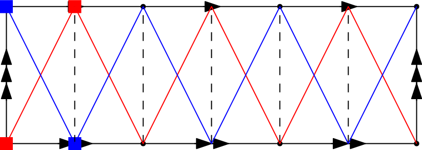
We first identify the faces of this complex by the product set \([2]\times [\ell]\), where the index \((i,j)\) corresponds to the face in the \((i+1)\cdot (j+1)\)-th position, when counting from left to right in Figure 6. We can see that each vertex is incident to all the \(2\ell\) faces. The associated \(2\ell\) edges of the diagonal graphs \(\mathcal{G}_X^\Box\) and \(\mathcal{G}_Z^\Box\) inherit the indexing of the faces of \(\mathcal{S}_\ell\).
4.2.0.2 Local codes.
To construct local codes, we first consider \(\mathscr{C}_2(1+X)\), the repetition code of length \(2\), and \(\mathscr{C}_\ell(g)\), the cyclic code of length \(\ell\) generated by \(g\). We define the tensor code \(\Pi_X, \Pi_Z\subseteq \mathbb{F}_2^{2}\otimes\mathbb{F}_2^{\ell}\), where \[\begin{align} \Pi_X&=\mathscr{C}_2(1+X)\otimes\mathscr{C}_\ell(g), \\ \Pi_Z&=\mathscr{C}_2(1+X)\otimes\mathscr{C}_\ell(g)^\perp, \end{align}\] and \(\mathbb{F}_2^{2}\otimes\mathbb{F}_2^{\ell}\) is endowed with the canonical product basis indexed by \([2]\times [\ell]\), as described in Section 2.6. We will subsequently justify this particular choice of product codes.
4.2.0.3 Definition of \(C_X\).
We start by defining a classical Tanner code associated to \(\mathcal{G}_X^\Box\). The graph \(\mathcal{G}_X^\Box=(V_X,F)\) has only two vertices, \(V_X=\{x_{0},x_{1}\}\), as shown in Figure 6. The edge-neighborhood of these vertices, in the graph, is equal to their face-neighborhood in the complex \(\mathcal{S}\), and \(F(x_{0})=F(x_{1})=F\).
We notice a natural local product structure relative to the vertices of \(V_X\). These are defined by the bijections \[\phi_{x_0}:\begin{cases} \hfill F\hfill&\to [2]\times [\ell]\\ (i,j)&\mapsto (i,i+j \operatorname{mod} \ell),\\ \end{cases} \quad \text{and} \quad \phi_{x_1}:\begin{cases} \hfill F\hfill&\to [2]\times [\ell]\\ (i,j)&\mapsto (i,j). \end{cases}\] Each local code associated to these vertices is set to be isomorphic to the dual of the tensor code \(C_{x_t}\cong \Pi_X^\perp\), \(t=0,1\). For \(t=0\), the isomorphism is induced by extending \(\phi_{x_0}\) by linearity into \(\phi_{x_0}:\mathbb{F}_2 F \to \mathbb{F}_2^{2}\otimes\mathbb{F}_2^{\ell}\) sending faces to the canonical basis vectors, where our choices of indexing for basis elements in the case of product codes and cyclic codes are described in Section 2.6. Similarly, we obtain the bijection \(\phi_{x_1}:\mathbb{F}_2 F \to \mathbb{F}_2^{2}\otimes\mathbb{F}_2^{\ell}\). This completes the characterization of the local codes \(C_{V_X}=(C_{x_i})_{i \in \{0,1\}}\) and of the classical Tanner code \(C_X := T(\mathcal{G}_X^\Box,C_{V_X})\).
4.2.0.4 Definition of \(C_Z\).
The classical Tanner code associated to \(\mathcal{G}_Z^\Box\) is defined similarly. The graph \(\mathcal{G}_Z^\Box=(V_Z,F)\) also has two vertices, \(V_Z=\{z_{0},z_{1}\}\), which are incident to all the faces, i.e., \(F(z_{0})=F(z_{1})=F\). Each local code associated with these vertices is set to be isomorphic to the dual of the same tensor code, \(C_{z_t}\overset{\phi_{z_t}}{\cong }\Pi_Z^\perp\) where each isomorphism is induced by \(\phi_{z_t}=\phi_{x_t}\), for \(t=0,1\). This completes the characterization of \(C_{V_Z}=(C_{z_i})_{ i\in \{0,1\}}\) and \(C_Z := T(\mathcal{G}_Z^\Box,C_{V_Z})\).
4.2.0.5 Orthogonality condition.
Let us now explain in words why the code \(\operatorname{CSS}(C_X,C_Z)\) is well-defined. The first factor of each product code \(\Pi_X,\Pi_Z\) is a repetition code to ensure that the checks associated with \(x_0\) and \(x_1\) commute with the checks associated with the vertices \(z_0\) and \(z_1\), respectively.
Moreover, due to the identification of the left and right edges of the presentation complex, our local product structure is not strict. To remedy this problem, the linear codes need to have a cyclic symmetry in order for a check associated with \(x_0\) to commute with one associated with \(z_1\). More precisely, with our choice of indexing, a codeword \(c_x=(1,1)\otimes c\), representing a \(X\)-check, and a codeword \(c_z=(1,1)\otimes c'\), representing a \(Z\)-check, are orthogonal to each other if \[\langle c,c'\rangle +\langle c,\rho(c')\rangle=0,\] where the rotation map \(\rho\) is defined in Section 2.6. This can be written as \(\langle c,c'+\rho(c')\rangle=0\), which is automatically satisfied if the second factor of \(\Pi_X\) and \(\Pi_Z\) are a cyclic code and its dual, respectively. Overall, these conditions ensure that \(C_X^\perp\subseteq C_Z\).
4.2.0.6 Parity-check matrices.
Another way to describe \(C_X\) and \(C_Z\) is by the kernels of parity-check matrices \(H_X\) and \(H_Z\), as explained in Section 2.4. We denote \(h\) the check polynomial of \(\mathscr{C}_\ell(g)\). In a certain basis, the parity-check matrix can be written \[\begin{align} H_X=\left[\begin{array}{c|c} \mathbb{G}( Xg(X)) & \mathbb{G} (g(X))\\ \hline \mathbb{G} (g(X)) & \mathbb{G}( g(X)) \end{array}\right], \quad \quad H_Z=\left[\begin{array}{c|c} \mathbb{G}( \bar h(X)) & \mathbb{G} (\bar h(X))\\ \hline \mathbb{G} (X\bar h(X)) & \mathbb{G}( \bar h (X)) \end{array}\right]. \end{align}\]
It is straightforward to verify that \(H_X\cdot H_Z^T=0\), using that \(\mathbb{G}( Xg(X))\) is a cyclic permutation of \(\mathbb{G}( g(X))\), and that \(\mathbb{G}(g(X)) \mathbb{G}(\bar h(X))^T=0\).
4.2.0.7 Code lifting.
Now that we have described quantum Tanner codes constructed on the square complex \(\mathcal{S}_\ell\), we can consider their lifts, as given in Section 3.2. Our first objective is to prove that our construction behaves well under lifting.
Proposition 6. Let \(p:\tilde{\mathcal{S}}_\ell\to \mathcal{S}_\ell\) be a covering map and \(\tilde{C}_X=T(\tilde{\mathcal{G}}_X^\Box ,C_{\tilde{V}_X})\), \(\tilde{C}_Z=T(\tilde{\mathcal{G}}_Z^\Box ,C_{\tilde{V}_Z})\), the lifted classical Tanner codes associated to \(p\). Then \(\tilde{C}_X^\perp\subseteq \tilde{C}_Z\).
Proof. Our objective is to determine the intersection of the face neighborhood \(F(\tilde{x}_s)\cap F(\tilde{z}_t)\), for any pair of vertices \(\tilde{x}_s\in p^{-1}(x_s)\) and \(\tilde{z}_t\in p^{-1}(z_t)\), \(s,t\in \{0,1\}\), and show that the support intersection of any \(X\)- and \(Z\)-checks associated with these vertices is of even size. By symmetry of the code structure, it is sufficient to verify this condition for pairs \((\tilde{x}_0,\tilde{z}_0)\) and \((\tilde{x}_0,\tilde{z}_1)\) in \(\tilde{S}_\ell\).
It is clear that any adjacent vertices \(\tilde{x}_0,\tilde{z}_0\) share at least 2 faces, which are attached to an edge \(\tilde{e}=\{\tilde{x}_0,\tilde{z}_0\}\), drawn vertically on Figure 6. Since an \(X\)-check is a codeword of the product code \(\Pi_X\), if it acts on the qubit associated to one of the two faces, then it must also act on the other, and similarly for a \(Z\)-check. Therefore, the support of an \(X\)- and \(Z\)-check associated with the vertices \(\tilde{x}_0\) and \(\tilde{z}_0\), respectively, must intersect on an even number of qubits.
A pair of adjacent vertices of the form \(\tilde{x}_0,\tilde{z}_1\) are connected by an edge incident to \(\ell\) faces in \(\tilde{S}_\ell\). The restriction of the support vector of an \(X\)-check associated with \(\tilde{x}_0\) on these faces is a codeword of \(\mathscr{C}_\ell(g)\), while that of a \(Z\)-check associated \(\tilde{z}_1\) is a codeword of \(\mathscr{C}_\ell(g)^\perp\). These vectors being orthogonal, their support intersection is even. ◻
| \(\ell\) | \(W\) | Lift index | \(\operatorname{deck}(p)\) | \([[n,k,d]]\) | \(d^2/n\) |
|---|---|---|---|---|---|
| 10 | 4 | 1 | \(1\) | \([[20,2,2]]\) | 0.2 |
| 20 | \(D_{20}\), \(\mathbb Z_5 \rtimes \mathbb Z_4\) | \([[400,2,20]]\) | 1 | ||
| 14 | 12 | 1 | \(1\) | \([[28,2,6]]\) | 1.25 |
| 4 | \(\mathbb Z_2 \times \mathbb Z_2\), \(\mathbb Z_4\) | \([[112,2,12]]\) | 1.25 | ||
| 7 | \(\mathbb Z_7\) | \([[196,2,18]]\) | 1.65 | ||
| 16 | \(\mathbb Z_4 \rtimes \mathbb Z_4\), \(\mathbb Z_8 \rtimes \mathbb Z_2\), \(Q_{16}\) | \([[448,2,24]]\) | 1.25 | ||
| 28 | \(\mathbb Z_{28}\) | \([[784,2,36]]\) | 1.65 |
To illustrate this construction, we instantiate the case \(\ell=10\) and \(\ell=14\) in the examples below, and we summarize the parameters of selected lifted codes in Table 1.
Example 1. The instances for \(\ell=10\) in Table 1 are obtained for a cyclic code \(\mathscr{C}_\ell(g)\) with generating polynomial \(g(X)=1+X^5\), and check polynomial \(h(X)=g(X)\). Used as a local code, this produces Tanner codes with check-weight 4. As in the Tanner version of the toric code, they could be seen as rotated versions of certain topological codes.
Example 2. The instances for \(\ell=14\) in Table 1, are obtained by using the shortest example of non-trivial cyclic self-dual binary code [24]. This has parameters \([14,7,4]\), and is generated by the polynomial \[g(X)=(X+1)(X^3 +X+1)^2=1+X+X^2+X^3+X^6+X^7.\] The generator matrix associated to \(g\) has row-weight \(6\), but by elementary operations, we can turn it into a full-rank generator matrix with \(6\) rows of weight \(4\), and one row of weight \(6\). This means that for the associated quantum Tanner code and its lifts, one-seventh of the checks are of weight \(12\) and the others are of weight \(8\). We emphasize that the last four lines of Table 1 represent LDPC codes with distance \(d>\sqrt{n}\).
Remark 7. In the base code, an \(X\)- and a \(Z\)-check overlap on all the qubits, while in the lifted code, their overlap must be reduced, otherwise the square complex would not remain connected. This shows that these codes, which do not satisfy the assumption of Proposition 2, constitute examples of lifts beyond the technique of [2], where lifting a code preserved the size of the overlap between any pair of \(X\)- and \(Z\)-checks.
4.3 Quantum Tanner code with double-circulant local code↩︎
![Figure 8: Left: presentation complex M_\ell of \operatorname{BS}(\ell,\ell) for \ell=3. Right: its subdivision into a bipartite square complex \mathcal{S}_3, and the indexing of the faces by (i,j,\kappa)\in[4]\times \mathbb{[}\ell]\times \mathbb{[}2].](/article/2502.20297/Quantum_Tanner_BS.png "fig:")
Our second construction is based on the presentation complex \(M_\ell\) of the Baumslag-Solitar group defined as \[\operatorname{BS}(\ell,\ell)=\langle a,b | ab^\ell a^{-1}b^{-\ell}\rangle,\] where \(\ell \in \mathbb{N}\), combined with a set of local tensor-product codes.
4.3.0.1 Square complex.
The presentation complex of \(\mathrm{BS}(\ell)\) is constructed on the model of Figure 6, which is for \(\ell=3\). For higher values of \(\ell\), we identify \(\ell\) segments along the top and \(\ell\) along the bottom. The presentation complex always has two directed edges, \(e_a\) and \(e_b\), associated with the generators \(a\) and \(b\) of the group presentation, respectively. It is modified into a bipartite square complex by subdividing the unique face into two rows of \(4\ell\) square faces. This process also subdivides the horizontal edge \(e_b\) into four edges (indexed by \([4]\)), and the vertical edge \(e_a\) into two edges (indexed by \([2]\)). This also adds new new horizontal and vertical edges. This forms the bipartite square complex \(\mathcal{S}_\ell := (V=V_X\sqcup V_Z,E,F)\) having \(|V|=4\ell+4\), \(|E|=8\ell+4\), and \(|F|=8\ell\). Each new vertex of the subdivided edge \(e_b\) is incident to \(4\ell\) faces, and each vertex along the middle cycle of edges is incident to 4 faces. The two diagonal graphs \(\mathcal{G}_X^\Box\) and \(\mathcal{G}_Z^\Box\) of \(\mathcal{S}_\ell\) are depicted in Figure 7
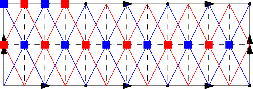
We identify the faces of this complex with elements of the product set \([4]\times [\ell]\times [2]\), where \((i,j,\kappa)\) represents the face in the upper row if \(\kappa=0\) and in the upper row if \(\kappa=1\), placed in the \((i+1)\cdot (j+1)\)-th position when counting from left to right in Figure 8. The face \((i,j,\kappa)\) is therefore incident to the edge indexed \(i\) in the subdivision of \(e_b\). The \(8\ell\) edges of the diagonal graphs \(\mathcal{G}_X^\Box\) and \(\mathcal{G}_Z^\Box\) inherit the indexing of the faces of \(\mathcal{S}_\ell\).
4.3.0.2 Local codes.
To construct the local codes, we consider \(\mathscr{C}_2(1+X)\), the repetition code of length \(2\), and the double-circulant code \(\mathscr{D}_{2\ell}(f)\), with polynomial \(f\in R_\ell\). We define the tensor codes \(\Pi_X, \Pi_Z\subseteq \mathbb{F}_2^{2}\otimes\mathbb{F}_2^{2\ell}\), where \[\begin{align} \Pi_X&=\mathscr{C}_2(1+X)\otimes\mathscr{D}_{2\ell}(f) \\ \Pi_Z&=\mathscr{C}_2(1+X)\otimes\mathscr{D}_{2\ell}(f)^\perp. \end{align}\] Recall that \(\mathbb{F}_2^{2}\otimes\mathbb{F}_2^{2\ell}\) is endowed with the product basis indexed by the set \([2]\times [2\ell]\) as described in Section 2.6. We will subsequently justify why this particular choice of product codes ensures orthogonality of \(X\)- and \(Z\)-checks.
4.3.0.3 Definition of \(C_X\).
We first define a classical Tanner code on \(\mathcal{G}_X^\Box=(V_X,F)\), where \(V_X=(x_i)_{i\in [2\ell+2]}\). This graph has two-vertices of degree \(4\ell\), labeled \(x_0\) and \(x_1\), which result from subdividing the edge \(e_b\). Their edge neighborhood in \(\mathcal{G}_X^\Box\) is equal to their face neighborhood in \(\mathcal{S}_\ell\), and they satisfy \(F(x_{0})\cap F(x_{1})=\emptyset\), \(F(x_{0})\cup F(x_{1})=F\).
We notice a natural local product structure relative to the vertices of \(V_X\). These are defined by the bijections \[\phi_{x_0}:\begin{cases} \hfill F(x_0)\hfill&\to [2]\times [2\ell]\\ (0,j,\kappa)&\mapsto (0,\kappa\ell +j)\\ (3,j,\kappa)&\mapsto (1,\kappa\ell + (j+1\operatorname{mod}\ell)) \end{cases} \quad \text{and} \quad \phi_{x_1}:\begin{cases} \hfill F\hfill&\to [2]\times [\ell]\\ (i,j,\kappa)&\mapsto (i\operatorname{mod}2,\kappa\ell +j). \end{cases}\] Each local code associated with these vertices is set to be isomorphic to the dual of the tensor code \(C_{x_t}\cong \Pi_X^\perp\), where the isomorphism is obtained by extending \(\phi_{x_t}\) by linearity into \(\phi_{x_t}:\mathbb{F}_2 F(x_t) \to \mathbb{F}_2^{2}\otimes\mathbb{F}_2^{2\ell}\) for \(t=0,1\), sending each face to a canonical basis vectors.
The graph \(\mathcal{G}_X^\Box\) also has \(2\ell\) vertices of degree \(4\), labeled \(x_t\), \(t=2,\dots, 2\ell+1\). They belong to the central horizontal cycle of edges, as shown in Figure 8. For all of them, we set \(C_{x_t}\) to be the parity code of length 4, i.e. the single parity check assigned to vertex \(x_t\) has full support over its face neighborhood \(F(x_t)\) in \(\mathcal{S}_\ell\). This completes the characterization of \(C_{V_X}=(C_{x_i})_{i\in [2\ell+1]}\) of the classical Tanner code \(C_X := T(\mathcal{G}_X^\Box,C_{V_X})\).
4.3.0.4 Definition of \(C_Z\).
The classical Tanner code associated to \(\mathcal{G}_Z^\Box\) is defined similarly. The graph \(\mathcal{G}_Z^\Box=(V_Z,F)\), where \(V_Z=\{z_i,\:i\in [2\ell+2]\}\), has two vertices of degree \(4\ell\) labeled \(z_0\) and \(z_1\). They satisfy \(F(z_{0})\cap F(z_{1})=\emptyset\), \(F(z_{0})\cup F(z_{1})=F\).
We notice again a natural local product structure relative to the vertices of \(V_Z\), that is defined by the bijections \[\phi_{z_t}:\begin{cases} F(z_t)&\to [2]\times [2\ell]\\ (i,j,\kappa)&\mapsto (i\operatorname{mod}2,\kappa\ell +j), \end{cases}\] for \(t=0,1\). For each of these vertices, we define a local code \(C_{z_t}\cong\Pi_Z^\perp\), where this isomorphism is obtained by extending \(\phi_{z_t}\) into a map \(\phi_{z_t}:\mathbb{F}_2 F(z_t) \to\mathbb{F}_2^{2}\otimes\mathbb{F}_2^{2\ell}\). The graph \(\mathcal{G}_Z^\Box\) has also \(2\ell\) vertices of degree \(4\), labeled \(z_t\), \(t=2,\dots ,2\ell+1\). They belong to the central horizontal cycle of edges, as depicted in Figure 8. For them, we set \(C_{z_t}\) to be the parity code of length 4. This completes the characterization of \(C_{V_Z}=(C_{z_i})_{i\in [2\ell+1]}\) and \(C_Z := T(\mathcal{G}_Z^\Box,C_{V_Z})\).
4.3.0.5 Orthogonality condition.
We next explain why the code \(\operatorname{CSS}(C_X,C_Z)\) is well-defined. To begin with, the first factor of the product codes \(\Pi_X,\Pi_Z\) is a repetition code to ensure that the checks associated with \(x_t,z_t,t=0,1\) commute with the middle checks, those for \(t=2,\dots ,2\ell+1\).
Next, due to the identification of the left and right edges of the presentation complex, our local product structure is not strict. To resolve this issue, the second linear codes must have a simultaneous cyclic symmetry for \(\kappa=0,1\) so that a check associated with \(x_0\) commutes with one associated with \(z_1\). To be precise, following our choice of indexing for the local codes, the condition for a codeword \(c_x=(1,1)\otimes c\), representing an \(X\)-check, and a codeword \(c_{z}=(1,1)\otimes c'\), representing a \(Z\)-check, to be mutually orthogonal is \[\langle c,c'\rangle=0\:\text{and}\:\langle \sigma(c),c'\rangle=0,\] where the map \(\sigma\) is defined in Section 2.6. This is automatically satisfied if the second factor of \(\Pi_X\) and \(\Pi_Z\) are a double-circulant code and its dual, respectively. The two conditions above thus ensure \(C_X^\perp\subseteq C_Z\).
4.3.0.6 Code lifting.
Now that we have described quantum Tanner codes constructed over the square complex \(\mathcal{S}_\ell\), we can consider their lifts, as in Section 3.2. Our first objective is to prove that our construction behaves well under the operation of code lifting.
Proposition 8. Let \(p:\tilde{\mathcal{S}}_\ell\to \mathcal{S}_\ell\) be a covering map and \(\tilde{C}_X=T(\tilde{\mathcal{G}}_X^\Box ,C_{\tilde{V}_X})\), \(\tilde{C}_Z=T(\tilde{\mathcal{G}}_Z^\Box ,C_{\tilde{V}_Z})\) be the lifted classical Tanner codes associated to \(p\). Then \(\tilde{C}_X^\perp\subseteq \tilde{C}_Z\).
Proof. Our objective is to determine the intersection of the face neighborhood \(F(\tilde{x}_s)\cap F(\tilde{z}_t)\), for any pair of vertices \(\tilde{x}_s\in p^{-1}(x_s)\) and \(\tilde{z}_t\in p^{-1}(z_t)\), \(s,t\in \{0\dots 2\ell+1\}\), and show that the support intersection of any \(X\)- and \(Z\)-checks associated with these vertices is of even size. By symmetry of the code, it is sufficient to check for pairs \((\tilde{x}_0,\tilde{z}_0)\) and \((\tilde{x}_0,\tilde{z}_2)\) in \(\tilde{S}_\ell\).
It is clear that any adjacent vertices \(\tilde{x}_0,\tilde{z}_2\) are incident to either two or four common faces. It is possible to partition this set of faces into pairs of adjacent faces and sharing an edge \(\tilde{e}\) whose image by \(p\) is an edge \(\{x_0,z_2\}\) represented vertically in Figure 8. Since an \(X\)-check is a codeword of the product code \(\Pi_X=\mathscr{C}_2(1+X)\otimes\mathscr{D}_{2\ell}(f)\), if it acts on the qubit associated with one of the two faces of a given pair, then it must also act on the other. Moreover, a \(Z\)-check has full support on the qubits associated to the face neighborhood of \(\tilde{z}_2\) . Therefore, the support of an \(X\)-and a \(Z\)-check associated with the vertices \(\tilde{x}_0\) and \(\tilde{z}_0\), respectively, must intersect on an even number of qubits.
A pair of adjacent vertices of the form \(\tilde{x}_0,\tilde{z}_1\) are connected by an edge incident to \(2\ell\) faces in \(\tilde{S}_\ell\). The restriction of the support vector of an \(X\)-check associated with \(\tilde{x}_0\) is a codeword of \(\mathscr{D}_{2\ell}(f)\) on these \(2\ell\) faces, while that of a \(Z\)-check associated with \(\tilde{z}_1\) is a codeword of \(\mathscr{D}_{2\ell}(f)^\perp\). These vectors being orthogonal, their support intersection is even. ◻
| \(\ell\) | \(W\) | lift index | \(\operatorname{deck}(p)\) | \([[n,k,d]]\) | \(d^2/n\) |
|---|---|---|---|---|---|
| 3 | 6 | 1 | \(1\) | \([[24,0,\infty]]\) | \(\infty\) |
| 12 | \(\mathbb Z_{12}\), \(D_{12}\), \(\mathbb Z_3 \rtimes \mathbb Z_4\) | \([[288,4, 6]]\) | 0.125 | ||
| 24 | \(\mathbb Z_2\times (\mathbb Z_3 \rtimes \mathbb Z_4)\), | \([[576,4,24]]\) | 1 | ||
| \(\mathbb Z_3 \rtimes \mathbb Z_8\), \(\mathbb Z_4\times S_3\) | |||||
| 4 | 8 | 1 | \(\{e\}\) | \([[32,2,4]]\) | 0.5 |
| 3 | \(\mathbb Z_3\) | \([[96,2,12]]\) | 1.5 | ||
| 5 | \(\mathbb Z_5\) | \([[160,2,16]]\) | 1.6 |
![Figure 10: Covering space of the square complex \mathcal{S}_4 associated to the group \mathbb{Z}_3 in Table 2 and Example 4. Directed edges with an arrow of the same color and type are identified. The support of an X-stabilizer associated with the local code defined in \tilde{x}_1\in p^{-1}(x_1) is represented by the eight gray faces. The other checks of weight 8 are obtained by cyclic shifts of this pattern. Each vertex of the middle cycle supports a check of weight four (on its entire face neighborhood). This leads to the code with parameters [[96,2,12]]. This figure directly provides a planar layout of the physical qubits.](/article/2502.20297/Quantum_Tanner_BS_1_quantumchip_svg-tex.png "fig:")
We examine two specific instances and their lifts in the examples below, for \(\ell=3\) and \(\ell=4\). We list the parameters of selected lifted codes in Table 2.
Example 3. The smallest non-trivial quantum Tanner code arises for \(\ell=3\). In Table 2, the double-circulant code used in the tensor product is either the \([6,3,3]\) code \(\mathscr{D}_{6}(f)\) with \(f(X)=X+X^2\), or its dual. In this case, we notice that the quantum Tanner code has zero dimension. However, by lifting it, we find codes of check weight \(6\) with positive dimension.
The following example, corresponding to the last three rows of Table 2 constitutes our best lifted codes.
Example 4. The case \(\ell=4\) in Table 2 is obtained by using the shortest example of non-trivial double circulant self-dual binary code. This is the \([8,4,4]\) extended Hamming code \(\mathscr{D}_8(f)\) with \(f(X)=X+X^2+X^3\). The generator matrix of \(\mathscr{D}_8(f)\) has row-weight 4, meaning that each of the classical Tanner codes \(C_X\) and \(C_Z\) has 16 parity checks, 8 of which being of weight \(8\). The other 8 are defined on vertices indexed by \(t=2,\dots, 9\) and are checks of parity codes of weight \(4\). The weights of the parity-checks are found in the same proportions in the lifted codes. We emphasize that in the last two lines of Table 2, the codes are obtained by cyclic lifts, and their distances satisfy \(d>\sqrt{n}\).
In Figure 10, we illustrate the covering of \(\mathcal{S}_4\) associated with the \([[96,2,12]]\) code. Because of the symmetry of the non-local checks, all obtained by cyclic shifts of the one represented in the figure, this may provide a biplanar layout of the physical qubits suitable for experimental implementation. We leave a rigorous analysis for future work.
Remark 9. The codes introduced in this section do not satisfy the assumption of Proposition 2 and also constitute examples beyond the lifting technique of [2], similarly to those described in Remark 7.
Propositions 5 and 3 can be applied to the last two codes of Table 2, corresponding to Example 4. In those cases, the codes with parameters \([[96,2,12]]\) and \([[160,2,16]]\) are index-\(t\) lifts with \(t=3\) and \(t=5\), respectively, and the group of deck transformations is \(\Gamma=\mathbb{Z}_t\). Using Proposition 5, we obtain a lower bound on the parameters of these codes, which is consistent with \(k=2\). Moreover, since in those cases lifting preserves the dimension of the base code, \(\pi^*\) and \(\tau_*\) are isomorphisms. Therefore, the logical operators, which correspond to classes in \(H^i(\tilde{C})\) and \(H_i(\tilde{C})\), respectively, are invariant under cyclic permutations of \(\Gamma\). Finally, the \([[96,2,12]]\) code saturates the distance upper bound given by Proposition 3.
Acknowledgement↩︎
The first author would like to thank Benjamin Audoux and Anthony Leverrier for valuable discussions throughout this work. We acknowledge the Plan France 2030 through the project NISQ2LSQ ANR-22-PETQ-0006.
5 Connected covering of a square-complex↩︎
In this section, we describe a procedure to explicitly construct a connected covering of a square-complex, which was introduced in [2]. It is based on the voltage assignment technique of [3], [16] and adapted from [14], [15] to generate connected covering maps.
We consider a connected square-complex \(\mathcal{S}=(V,E,F)\) which has finitely many cells. Recall that the graph \(\mathcal{G}=(V,E)\), can be seen as the 1-skeleton of \(\mathcal{S}\). The fundamental group of a square-complex is defined in Section 2.1.
From the Galois correspondence, Theorem 1, connected coverings of \(\mathcal{S}\) are in one-to-one correspondence with subgroups of \(\pi_1(\mathcal{S},v)\), where \(v\) is an arbitrary choice of basepoint that we later omit. Let \(H\) be a subgroup of \(\pi_1(\mathcal{S})\). There exists a unique covering map, \[\label{equation32covering} p:\mathcal{S}_H \rightarrow \mathcal{S},\tag{4}\] associated to \(H\), and it has index \(r=[\pi_1(\mathcal{S}):H]\). To construct the covering above we will construct one for \(\mathcal{G}\). For that, we have to consider the following subgroups and homomorphisms, \[\begin{tikzcd}[column sep=0cm, row sep=0.6cm] & \pi_1(\mathcal{S}) & \geq & H \arrow{d}{\phi^{-1}} \\ & \pi_1(\mathcal{G}) \arrow{u}{\phi} & \geq & H^1 \end{tikzcd},\] where \(\phi\) is the natural homomorphism taking the quotient of \(\pi_1(\mathcal{G})\) by the normal closure of the subgroup generated by relations coming from 4-cycles in \(\mathcal{S}\). Moreover, \(H^1\) is the preimage of \(H\) in \(\pi_1(\mathcal{G})\) by this homomorphism. We now denote \(\Gamma:=\pi_1(\mathcal{K} )/H\) and \(\Gamma^1:=\pi_1(\mathcal{G})/H^1\). When \(H\) is normal, \(\Gamma\)and \(\Gamma^1\) are isomorphic, otherwise this is a bijection between the cosets (here, all cosets are taken on the right).
To construct the covering map of Equation 4 , it is shown in [15] that we only need to construct the following covering, \[\label{Equation32covering32of321-skeleton} p_{1}:\mathcal{G}_{H^1}\rightarrow \mathcal{G},\tag{5}\] which is unique by Theorem 1 .
We explain the steps to create the components of Equation 5 , and we detail a combinatorial technique specifically designed to produce connected coverings. The graph \(\mathcal{G}_{H^1}\) has a set of vertices \(V\times \Gamma^1\), and set of edges in bijection with \(E\times \Gamma^1\). We now describe how to connect the edges. Since \(\mathcal{G}\) is a connected graph, it admits a maximal spanning tree \(T\) with basepoint \(v\), and by definition a unique reduced path from vertex to vertex. We denote \(E^*\) the set of oriented edges (its cardinality is twice the one of \(E\)).
We define a map called voltage assignment on the set of oriented edges, \[\label{Equation32modified32voltage32assignment} \nu^T: E^* \to \pi_1(\mathcal{G}),\tag{6}\] mapping an edge \(e=[v_1,v_2]\) to an element of \(\pi_1(\mathcal{G})\) in the following manner. Let a path \(\alpha\) from vertex \(a\) to \(b\) be denoted as a sequence of oriented edges, for example \(\alpha=[a,u_1].[u_1,u_2]\dots [u_j,b]\). Moreover, let \(((a,b))\) denote the path from \(a\) to \(b\) in the tree \(T\). Then the equivalence class of circuits obtained by adding \(e\) to \(T\) is \(\nu^T(e):=[((v,v_1)).e.((v_2,v))]\), where \([\alpha]\) is the standard notation for the homotopy class of a circuit \(\alpha\) based at \(v\).
We define a connected lift of the graph \(\mathcal{G}\) associated to a certain subgroup of its fundamental group, using the notation above.
Definition 4 (Connected lift of a graph). The lift of \(\mathcal{G}\) associated to the subgroup \(H^1\leq \pi_1(\mathcal{G})\) is the graph \(\mathcal{G}_{H^1}\) with set of vertices \(V\times \Gamma^1\) and set of edges in bijection with \(E\times \Gamma^1\), so that a vertex or edge is written \((c,gH^1)\) with \(c\in \mathcal{G}\) and \(g\in \pi_1(\mathcal{G})\). An oriented edge \(\tilde{e}=(e,gH^1)\) in the graph \(\mathcal{G}_{H^1}\), with \(e=[u,v]\), connects \((u,gH^1)\) and \((v, g \nu^T(e)H^1)\), where the multiplication by \(\nu^T(e)\) is on the right.
When \(H^1\) is a normal subgroup of \(\pi_1(\mathcal{G})\), the resulting covering is Galois.
In general, a graph admits more than one spanning tree. Following this procedure with another choice of spanning tree will modify the parametrization of the vertices and edges, but the graphs will be isomorphic, by the Galois correspondence. If \(H^1\) is chosen as an arbitrary subgroup of \(\pi_1(\mathcal{G})\), it can be shown [2], [15] that Definition 4 can generate all connected regular and non-regular covers of \(\mathcal{G}\). We define \(p_{1}\) as the map projecting any cell of \(\mathcal{G}_{H_1}\), vertex or edge, to its first coordinate. This is a valid covering map, equivalent to what we have done in Section 2.3.
Here \(H^1\) is not arbitrary; it is the preimage of \(H\) by \(\phi\). It is also possible to prove that \(p_{1}\) induces an isomorphism \(p_{1\#}:\pi_1(\mathcal{G}_{H^1},\tilde{v})\to H^1\), for any choice of basepoint \(\tilde{v}\) in the preimage of \(v\), see [15], Chapter III. 3. Moreover, for a 4-cycle \(f\in F\), we can show that \(p_1^{-1}(f)\) is a set of \(r\) 4-cycles, and hence \(p_1\) can be extended into a covering of the square-complex \(\tilde{\mathcal{S}}:=(p_1^{-1}(V),p_1^{-1}(E), p_1^{-1}(F))\). It is finally proven in [15] that \(p_1\) induces an isomorphism \(p_{1\#}:\pi_1(\mathcal{S}_H,v')\to H\) so that \(p_H=p_1\) and \(\tilde{\mathcal{S}}=\mathcal{S}_H\).
References↩︎
Examples of gluing maps that are not homeomorphisms: the map \(\partial \mathbb{I} \to p\), mapping both end-points of an interval to the same point, yielding a 1D-sphere; the map \(\partial D^2\to p\), mapping the boundary of the disk, a circle, to a point, yielding a 2D-sphere.↩︎
This name suggests an analogy to the mixing of a deck of cards, which are called sheets in the context of covering spaces.↩︎
This theorem applies in a much broader context, but this is sufficient for our applications.↩︎
In the context of coverings of cell complexes, \(p_\#\) acts on chains of \(\mathbb{F}_2\tilde{E}\) and \(\mathbb{F}_2\tilde{V}\) in the cellular chain complex and is a chain map.↩︎
The closure of a set of faces is the subcomplex composed of those faces along with the set of vertices and edges incident to them.↩︎
The action of \(\gamma\) is naturally extended to the \(\mathbb{F}_2\)-space of the lifted codes.↩︎