An introduction to random rule-based chemical networks
January 01, 1970
Abstract
Large chemical networks appear in various branches of chemistry and biology, in particular, cellular metabolism and prebiotic chemistry. Detailed simulations of such networks are difficult, or even impossible for lack of kinetic data. Various strategies have been developed to produce synthetic random networks mimicking the large scale organizational properties of experimental chemical networks. These random networks are however mathematical artefacts, which fail to reflect the general reactivity structure of chemistry.
We present here a new class of random models of prebiotic (uncatalyzed) chemistry, based on context-independent rules, which is coherent with the general compositional logic of metabolism. The general organization of the random networks fits within the small world paradigm. We get a phase diagram of the models through an approximate mapping to a solvable tree growth model. Our predictions go beyond a purely abstract connectivity analysis of the reaction graph by studying the diversity of chemical mechanisms, and singling out evolutionary patterns, such as autocatalysis and multistationarity, paving the road to possible open-ended evolution.
1 General motivation↩︎
Understanding the chemical nature and general statistical features of large chemical reaction networks is a prominent question in Origin of Life studies. Historically, the first attempts to deal with the inherent complexity have come from the purely theoretical side: the theories of collectively autocatalytic sets (CASs), and reflexively autocatalytic, food-generated sets (RAFs), see [1], [2], [3], [4] have been used extensively to explore autocatalysis in relation to abiogenesis, following ideas originally due to Eigen and Schuster [5]. The later appearance of large databases of chemical reactions, such as KEGG [6], the metabolic network of Escherichia Coli [7], or the abiotic reaction database [8], and the simultaneous development of bioinformatic tools, have made possible an exploration of large networks of experimental origin, see e.g. [9], [10], [11], or [12] which discusses hierarchical network organization and possible evolution in terms of seed-dependent autocatalytic systems (SDAS), whereby an initial set of simple molecules (foodset) serves as initial generation of a multi-generation metabolic network obtained by recursively applying rules coming from various databases.
On the computational side, advanced DFT techniques have allowed the development of software like ChemKin [13] and RMG [14] in combustion chemistry, or more versatile algorithms like SCINE/Chemoton [15], YARP [16] and others, with applications to parametrization of the prebiotic chemistry space [17], [18]. Random sampling methods [19] have also been used for a rapid exploration of the chemical space. In parallel, ML techniques are aiding both the inference of effective kinetic rate laws from experiment and the computational exploration of chemical reaction networks, see e.g. [20], [21]. While DFT techniques allow rapid screening of reaction pathways and potential energy surfaces, the computational burden associated with high-precision functionals and accurate transition-state searches creates a fundamental trade-off between accuracy and throughput. Consequently, comprehensive exploration of very large chemical spaces remains beyond reach.
This has suggested the generation of synthetic random networks mimicking the large scale organizational properties of experimental chemical networks as an explorational tool, see [22] and refs. within. Graphs are typically sparse, but do not look like regular graphs, nor like the Erdős-Rényi random graph model. Several authors have tried to fit these (hyper)graphs to various models of random graphs [23], [24]. Other families of models have also been introduced, such as the "Small World" networks of Watts and Strogatz [25], or the Albert-Barabasi model of preferential attachment [26]. Metabolic networks are generally highly clustered, despite being sparse, and have a short characteristic path length due to a small number of ‘hubs’, i.e. metabolites with high connectivity, thus fitting qualitatively the small world paradigm [27]; a quantitative agreement, however, is not observed.
The abstract nature of the above random models makes them equally applicable to describe networks of very different nature (social networks, gene networks...) What is crucially missing here, from our point of view, is some chemically interpretable observable. Interesting questions from the chemist’s and biologist’s point of view, in a context of Origin of Life studies, may be: what are the main mechanisms producing long molecules with carbon skeletons ? Are they sufficiently diverse to produce a large enough set of biologically relevant molecules, but still selective enough to avoid the unhindered generation of the full set of organic molecules ? Are there any signatures of prebiotic dynamics, such as autocatalytic cycles or multistability, pointing to a possible proto-Darwinian evolution ? Is open-ended evolution to arbitrarily complex mechanisms possible ?
Elementary chemical knowledge suggests that mechanisms are based on context-independent assembly of functional groups. The MØD package [28] makes possible a systematic generation of pathways based on a fixed, finite grammar, i.e. non-random list of rules, instead of individual reactions, and stands in striking contrast to Erdös-Rényi type models, wherein each edge is accepted independently from the others.
We introduce here instead new classes of random network models, called random rule-based chemical networks, RRBCN for short. In a RRBCN, a primitive rule, if accepted, generates an infinite number of rules by context derivation, see Fig. 1 below for an illustration. Contrary to the MØD package, we provide random acceptation rules for mechanisms, which generate random, possibly infinite grammars. This procedure circumvents the task of enumerating all known mechanisms – which is error-prone, subject to interpretation and necessarily non-exhaustive –, and makes it possible to raise general questions about what any type of chemistry could be like, as a function of interpretable parameters. We argue that such models are robust, in the sense that dressing them with the main colors and specifics of biochemistry adds a few layers of complexity, but does not alter the general strategy and results outlined here, as discussed in the conclusion.
The rest of the section is devoted to an informal construction of the model, put against a general chemical context, and exposition of main results.
1.1 From chemical reactions to abstract rules↩︎
Synthesis chemistry is concerned with finding a synthesis path with best possible yield for a given compound. Expert knowledge collected by chemists over the years has allowed the discovery of a huge number of reaction paths producing millions of molecules; some of this knowledge has been collected into databases, most of them specific to a given branch (pharmacology, metabolism, etc.), see e.g. [6] or [29].
Because these databases are oriented towards synthesis goals, it is however fair to say that they fail to consider chemical networks in a systematic way, i.e. they do not provide a systematic, orderly set of chemical rules for reactivity. From common undergraduate knowledge, it is widely acknowledged that reactivity rules follow general mechanisms, based on the formation and breaking of bonds between moieties or functional groups (i.e., molecule fragments), and that these rules are widely independent on the context, i.e. on the group substituents (neighboring atoms), though kinetics, therefore yields, may depend on these to a considerable extent.
The point of view here is that of network expansion. The prototypal example is that of the famous ’52 Miller-Urey experiment, which demonstrated the synthesis of a large diversity (thousands of compounds) of organic compounds from inorganic constituents (in gaseous state, methane, ammonia, hydrogen and water vapor, supposed at the time to be representative of the archaic atmosphere of Earth) in an origin of life scenario; but other experimental sets have been considered and are under close scrutiny, see e.g. [30]. With modern-day computers, and using a chemical expertise on reaction mechanisms, one may contemplate describing the distribution of products inductively in terms of generations; see [12] for an example. Generation 0 is the set of organic constituents, often called foodset. The computer may consider all theoretical products of a priori plausible reaction mechanisms involving generation 0 compounds; those experimentally detected make up generation 1. Then, for every \(n\ge 2\), generation \(n\) compounds consists of all experimentally detected products of compounds of generations \(\le n-1\).
The key notion here is that of mechanisms or primitive reactions. Chemical rules, as envisioned in bioinformatics softwares such as [28], are context-independent, as opposed to individual database reactions, see e.g. [6]. This is perfectly standard for chemists, but let us provide an example for non-chemists (Fig. 1). An aldol reaction is any reaction of the above form, where \(R_1,R_2,R_3,R_4\) are placeholders for arbitrary groups. The numbering of carbon (C) atoms shows that this is an addition reaction, where two fragments are coalesced by making a bond. The underlying primitive reaction is obtained by considering only the reaction between the red parts (equivalently, by assuming trivial placeholders), \[\begin{align} && {\mathrm{(aldolization\;mechanism\;/\;primitive\;reaction)}} \nonumber \\ && \qquad O=C_3 + C_1-C_2=O \to O-C_3-C_1-C_2=O. \nonumber\\ \end{align}\] Aldolizations are the main rules0 driving the multiple steps of the autocatalytic formose cycle [31], [32], and participates in the Krebs cycle and other main metabolic cycles of life.
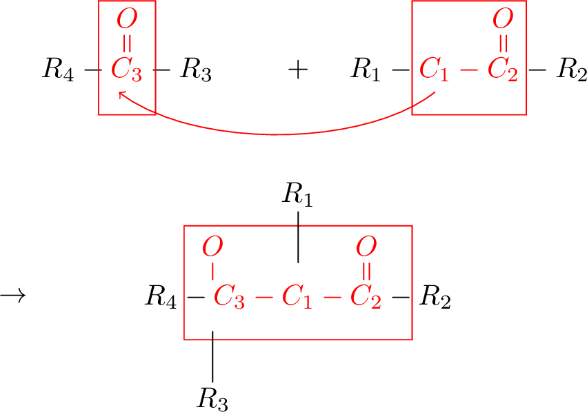
Addition reactions involve some electron rearrangement, which often manifests itself in bond displacements (here, the double bond \(O=C_3\) turned into \(O-C_3\)) or in charges. We simplify chemistry by
considering only addition rules and their reverses, fragmentation rules;
considering all bond types alike;
disregarding reactants or products with charges or cycles;
not discussing in full detail branching reactants or products (see below).
Molecular graphs have thus been turned into abstract words. Direct translation of reactivity rules such as the aldolization mechanism in this simplified language is not possible. However, coarse-graining functional groups such as \(O=C\) or \(O-C\) into an extra ‘atom’ denoted \(D\) suggests the simplified word addition (coalescence) rule \[R_4{\color{red}D_2} + {\color{red} CD_1}R_2 \longrightarrow R_4{\color{red} D_2CD_1}R_2 \label{eq:RCDR}\tag{1}\] which allows two free contexts \(R_4,R_2\) only. Eq. (1 ) is a rule derived (by context addition) from the primitive rule \[{\color{red}D_2} + {\color{red} CD_1} \longrightarrow {\color{red} D_2CD_1} \label{eq:CD}\tag{2}\] We tend to use the word rule instead of reaction in our model, though the two are used interchangeably. Note, however, that the primitive rule (2 ) allows \(R_4{\color{red} D_2}R_3\) to react with \(R_1 {\color{red} CD_1}R_2\) for arbitrary, non trivial \(R_3,R_1\), yielding a branching product.
In the following, we describe simplified models of reactivity satisfying these requirements, where molecules have become words with letters in an alphabet \(\cal A\) called atom set, and bonds have become word concatenation, denoted by a dot \((\cdot)\) or simple juxtaposition; words are identified by the word reversal symmetry, e.g. \(CD = DC\), a remnant of the graph symmetries involved in the SMILES representation of molecules [33]. We use upper case letters for atoms, and lower case letters for words, typically \(w,x\) or \(f\), possibly with lower indices.
1.2 Anabolic and catabolic rules, complexity indices↩︎
Metabolism is often organized into anabolic (synthetic) and catabolic (degradation) subsystems, the best-known examples of which being the Calvin cycle of photosynthesis vs. the Krebs cycle of respiration. The distinction between anabolic and catabolic reactions may have been essential in primordial metabolism, as has been put forward with much elegance and persuasive power by [34]. Anabolism allows the construction of long molecules with carbon skeleton, in general through simple addition rules (including e.g. aldolizations), wherein one of the reactants is a short molecule provided by the environment. Catabolism, on the other hand, cuts long molecules into short pieces by repeated fragmentations.
Here we specialize anabolism by assuming addition rules of the type \[{\mathbf{(anabolic\;rule)}} \qquad f+x\to f\cdot x,\] where \(f\in {\cal F}\) is in a fixed, finite set of molecules called external set, which would correspond to generation 0 in the above SDAS formalism. Catabolic rules are of the general fragmentation form \[{\mathbf{(catabolic\;rule)}}\qquad x_1\cdot x_2 \to x_1 + x_2.\] Both anabolic rules and catabolic rules are a priori reversible (and detailed balance should hold). To avoid interference between the two sets of rules, we assume that \(x,x_1,x_2\not\in {\cal F}\). Anabolic and catabolic rules together make up a set of rules called admissible rules.
The case when catabolic rules are irreversible corresponds to the dilute regime of open chemical reaction networks described in [35], where foodset species \(f\) are assumed to be abundant external species, and other species \(x\) are low-concentration internal species, making reverse reactions \(x_1+x_2\to x_1\cdot x_2\) of kinetic order 2 negligible. This linear regime is important, for it allows a direct interpretation of autocatalysis as instability of the trivial 0 fixed point, with dynamical growth rate equal to the highest eigenvalue (Lyapunov eigenvalue) of the generator of the dynamics.
The number of covalent bonds involved in an aldolization is 4 (the 4 red bonds on the right-hand side of Fig. 1); this means that letting the two reactants approach each other and form a bond involves a global reorganization of the associated electron orbitals. We say that the complexity index of such a reaction is 4, independently of the substituents \(R_1,R_2,R_3,R_4\); it is equal to the complexity of the underlying primitive reaction stripped of the \(R_i\). In our simplified model, we call
\(|x| =\) (number of atoms in \(x) - 1\)
the level of \(x\); it is also equal to the number of edges of the associated graph. Then the complexity index of a primitive anabolic rule \(\rho : f+x\to f\cdot x\), resp. catabolic rule \(x\to x_1\cdot x_2\), is \[m_{\rho} = |f|+|x|+1, \qquad {\mathrm{resp.}} \qquad m_{\rho} = |x|.\] The complexity index of rules derived from those is identical.
1.3 RRBCN Models: general construction↩︎
The kinetics of simple reactions not involving enzymes can in principle be modeled by mass-action kinetics, namely, the velocity of a reaction \(\rho: X_1+\ldots+X_n\to X'_1+\ldots+X'_{n'}\) is of the form \(k_{\rho}\) times the product \(\prod_{i=1}^n [X_i]\) of the concentrations of the reactants; the constant \(k_{\rho}\) is called kinetic rate. Within a given experiment, the reaction set may usually be split according to a finite number of rankings \((N_{\rho})_{\rho}\), from the fastest ones to the slowest ones. Those reactions that operate too slowly, typically because their kinetic rate is too low, are simply discarded as irrelevant. For simplicity, we discuss here only the case of an acceptation/rejection scheme: we choose a cut-off kinetic parameter \(k_{min}\) and let \[N_{\rho} = \begin{cases} 1, \qquad k_{\rho}>k_{min} \\ 0 \qquad {\mathrm{else}} \end{cases}\] Reaction rules with \(N_{\rho}=1\) are accepted, those with \(N_{\rho}=0\) are rejected. Here \((N_{\rho})_{\rho}\) are defined on the basis of independent, but not necessarily identically distributed, Bernoulli random variables \(\omega_{\rho}\); namely, \(N_{\rho}=1\) if and only if \(\omega_{\underline{\rho}}=1\) for some reaction \(\underline{\rho}\) from which \(\rho\) may be derived by adding context (including the case when \(\omega_{\rho}=1\)). The simplest possible models depend on \(\rho\) only through the complexity indices \(m_{\rho}\) defined in §1.2; namely, we let \(\mathbb{P}[\omega_{\rho} = 1]=p_{\rho}\), where \(p_{\rho} = p(m_{\rho})\) is a function of \(m_{\rho}\). This leads to the following formal definition of a network \(\bar{\cal R}\) drawn from a RRBCN (random rule-based chemical network) model, \[\begin{align} && \bar{\cal R} = \{\rho\;{\mathrm{admissible}}\;|\;N_{\rho} = 1\}, \nonumber\\ && \qquad N_{\rho} \overset{!}{=} \max_{\underline{\rho}\subset \rho} \omega_{\rho}, \qquad \omega_{\rho} \sim {\mathrm{Ber}}(p_{\rho}), \nonumber\\ && (\underline{\rho}\subset\rho) \Leftrightarrow \begin{cases} \underline{\rho}:\; f+x\to f\cdot x, \\ \qquad \rho: \;f+ x\cdot r \to f\cdot x\cdot r \;{\mathrm{(anabolic)}} \\ \underline{\rho}:\;x_1\cdot x_2 \to x_1 + x_2,\\ \;\; \rho: \;(r_1\cdot x_1)\cdot (x_2 \cdot r_2) \to r_1\cdot x_1 + x_2\cdot r_2 \\ \qquad \qquad {\mathrm{(catabolic)}} \end{cases} \nonumber\\ \label{eq:omega95rho} \end{align}\tag{3}\] in terms of Bernoulli random variables, where the max ranges over all admissible reactions \(\underline{\rho}\) from which \(\rho\) may be derived by adding (possibly trivial) contexts \(r,r_1,r_2\).
Such models differ from standard independent edge random graphs by a completion procedure. Namely, \(\cal R\) be the set of admissible reactions \(\rho\) such that \(\omega_{\rho}=1\). Then the reaction network, \(\overline{\cal R}\), is obtained from \(\cal R\) by adding all context derivations of reactions in \(\cal R\).
Fix a maximum level \(n_{max}\). For each admissible reaction \(\rho:f+x\to f\cdot x\) or \(x_1\cdot x_2\to x_1 + x_2\) with \(x,x_1,x_2\not\in {\cal F}\) and \(|f\cdot x|,|x_1\cdot x_2|\le n_{max}\), we generate an independent variable \(\omega_{\rho}\) as in (3 ). Then, for each admissible reaction \(\rho\), we let \(N_{\rho} \overset{!}{=} \max_{\underline{\rho}\subset \rho} \omega_{\underline{\rho}}\) as in (3 ). The resulting random network is denoted \(\bar{\cal R} = \bar{\cal R}(n_{max})\).
Instead of this two-stage process (global sampling of all Bernoulli variables, followed by completion by derivation), we use for simulations a more intuitive and much faster algorithm by induction on the level, which we describe for non-branching molecules. We construct at the same time a set Prim\((n)\) of primitive rules of the form \(f+x\to f\cdot x\) or \(x_1\cdot x_2\to x_1 + x_2\) with \(|f\cdot x|=n\), resp. \(|x_1\cdot x_2|=n\). Once the reaction sets \(\bar{\cal R}(n-1)\) and Prim\((n')\), \(n'=0,\ldots,n-1\) have been generated, \(\bar{\cal R}(n)\) is obtained from \(\bar{\cal R}(n-1)\) by adding level \(n\) rules of two types:
(inductive completion by derivation) adding derived rules \(f + x\cdot r \to f\cdot x\cdot r\), \((r_1\cdot x_1)\cdot (x_2\cdot r_2) \to r_1\cdot x_1 + x_2 \cdot r_2\) for all primitive reactions \(f+x\to f\cdot x\), resp. \(x_1\cdot x_2\to x_1 + x_2\) with \(|f\cdot x|<n\), resp. \(|x_1\cdot x_2|<n\);
(new primitive rules) defining Prim \((n)\) as those level \(n\) reactions \(\rho: f+x\to f\cdot x\), resp. \(x_1\cdot x_2\to x_1 + x_2\), not obtained by completion as in 1., such that \(|f\cdot x|=n\), resp. \(|x_1\cdot x_2|=n\), for which \(\omega_{\rho}=1\) (decide by tossing a coin with P(head) = \(p_{\rho}\)).
We still need to define a Bernoulli parameter \(p_{\rho}\) for each admissible rule \(\rho\).
1.4 RRBCN Models I and II↩︎
We consider in this work the following functional forms with three parameters \(0<p,q,z<1\):
(1) (constant parameter model, or Model I) \(p_{\rho} \equiv p\) (anabolic), \(p_{\rho}\equiv q\) (catabolic reaction), where \(0<p,q<1\) are constants;
(2) (constant affinity parameter model, or Model II) \(p_{\rho} \equiv p z^{m_{\rho}}\) (anabolic case), \(p_{\rho} \equiv q z^{m_{\rho}}\) (catabolic case), for some parameters \(0<p,q,z<1\). Parameter \(z\) is called affinity because it is conjugate to the complexity.
can be simply considered as random acceptation/rejection model for primitive reactions. A possible motivation for Model II (from which Model I can be gotten back by letting \(z\to 1\)) is the following. Model kinetic constants \(k_m\) of rules \(\rho\) in with complexity index \(m\) as \[k_m\sim k_{ref} \sigma^m U, \label{eq:km}\tag{4}\] where \(k_{ref}<k_{min}\) is some low kinetic value, \(0<\sigma<1\) is a cross-section-like parameter, and \(U\) is log-normal, namely, \(U \sim 10^{\lambda Z}\) (\(\lambda>0\)), \(Z\sim {\cal N}(0,1)\). Then accept \(\rho\) if \[k_m > k_{min} \label{eq:kmin}\qquad{(1)}\] for a certain kinetic threshold \(k_{min}\), and let \[p_{\rho} = q_{\rho}= {\mathbb{P}}[k_m>k_{min}] \label{eq:p61q}\tag{5}\]
The idea behind the parameter \(\sigma\) is that requiring an electron to move across \(m\) atoms has an average activation energy price roughly proportional to \(m\). The resulting rules can be mapped into a constant affinity parameter model in a certain regime of parameters; the parameter dictionary \((\frac{k_{min}}{k_{ref}}, \sigma, \lambda) \to (p,z)\) is spelled out in §I. A. of Suppl. Info.
It makes sense to postulate different values for \(p_{\rho}\) and \(q_{\rho}\); see §2.1.
1.5 Main results↩︎
We present in this work results of two very different types.
The first category of results are network-based explorations based on simulations (§ 2). The main emphasis here is on general connectivity features of the random networks (including sparsity, clustering, path lengths) and potential dynamical biosignatures (autocatalysis, multistability). Focusing on low-complexity mechanisms and low-level (short) molecules, typically up to 6-7 atoms, allows full-scale simulations. RRBCN networks are "Small-World" networks like extant metabolic networks, and their structure is rich enough to allow in principle autocatalysis and multistability. We say "in principle", because the direction (direct or reverse) of reactions, in- and out-fluxes of external molecules, and ultimately, kinetic rates, are not determined by the model, though they dictate the dynamical features that actually take place.
The second category of results are explorations of high-complexity mechanisms mostly based on theory (§3). The theoretical input is based on an approximate mapping to a solvable random tree growth model, which is particularly relevant to explore the high-level part of the networks. Partial simulations exploring long molecules (up to 30-50 atoms) prove excellent agreement with our predictions, but theory allows an exploration of regimes which are completely inaccessible by simulations. On the whole, we answer many questions raised in the Introduction relative to the diversity of high-complexity mechanisms, including the possibility of open-ended evolution, within the framework of our model.
Understanding proto-evolutionary dynamics would require to put together our two categories of results – notably, understand the organization of reaction subnetworks generated by the high-complexity mechanisms unveiled in §3. Some very partial results in that direction are presented in Suppl. Info., see introduction to Main Text, §3 for more.
A distinctive feature of our models is the comparatively small amount of independent random variables needed to define them – one per primitive rule –, because of automatic context completion. We get two limiting cases for Model II:
Letting \(p,z\to 0\) leaves only a small number of primitive rules. Then most likely the random graph is made up of small islands, and the average node connectivity is low.
Letting \(p,z\to 1\) also leaves only a small number of primitive rules. However, the random graph has most likely a high average node connectivity, with a giant connected component containing most molecules.
What is puzzling here is that both limits carry little diversity : all primitive rules have a low complexity index. The two cases differ by the fact that \(\bar{\cal R}\) contains few level \(n\) rules (compared to the number of admissible level \(n\) rules, for \(n\) large) when \(p,z\to 0\), as opposed to most level \(n\) rules when \(p,z\to 1\). Thus most level \(n\) rules in the latter case are deterministically derived from low-complexity primitive rules. Exploring intermediate regimes shows radical departure from independent edge random graph models, such as the Erdös-Rényi model. A detailed exploration of available mechanisms can be performed by analytical tools, based on auxiliary trees called composition for anabolism, or fragmentation trees for catabolism. Models I and II behave very differently, with Model I exhibiting only a finite (albeit potentially large) number of mechanisms, while there appears an infinite number of arbitrarily complex rules in some intermediate range of the Model II parameter \(z\), suggesting the possibility of open-ended evolution.
2 Exploration of low-level structure: connectivity and dynamics↩︎
In this section, we explore the model by simulations which focus on small-level cut-off random networks \(\bar{\cal R}(n_{max})\) with \(n_{max} = 6\) or \(7\) at most. The idea is to explore the shape and dynamical properties of a random network produced by a number of low-complexity mechanisms.
We have performed two types of network simulations: equilibrium network simulations (§2.1), focusing on the connectivity structure of the reaction graph; and out-of-equilibrium network simulations (§ 2.2), focusing on dynamical features.
2.1 Equilibrium network simulations : network connectivity↩︎
We assume here that admissible rules are reversible and that rates follow mass action and satisfy detailed balance.
Thermodynamic equilibrium for the anabolic reaction \(f+ x \overset{k}{\underset{\bar{k}}{\rightleftarrows}} f\cdot x\) commands that \(k /\bar{k} = e^{-\Delta G^0/RT}\), where \(\Delta G^0\) is the Gibbs energy of the reaction, and \((RT)^{-1}\) the temperature-dependent Gibbs parameter. We assume here a flat energy landscape for simplicity \((\Delta G^0\simeq 0)\), so that \(k\simeq \bar{k}\). Let \(C_0\), resp. \(C_1\) be a typical equilibrium concentration of external \(f\), resp. internal species \(x\). Given that \([f]\sim C_0\), the effective constant of the direct reaction is however \(\sim C_0 \bar{k}\) (see below). Similarly, given a reversible catabolic reaction \(x_1\cdot x_2 \overset{k}{\underset{\bar{k}}{\rightleftarrows}} x_1 + x_2\), we may assume that the effective constant of the reverse reaction is \(\sim C_1 k\).
The above effective constants allow a desymmetrization of the two rule types. Namely, letting \(\rho\) be a level \(m\) direct anabolic reactions, we define \(p_{\rho}\) by substituting the effective constant to the original one, namely, \(k_{ref}\to C_0 k_{ref}\) in (4 ); equivalently, \(\rho\) is accepted if \(k_m > k_{min}/C_0\), with \(k_m\) as in (4 ). Similarly, reverse level \(m\) catabolic rules are accepted if \(k_m > k_{min}/C_1\). Reverse anabolic or direct catabolic rules obey the original threshold relation (?? ). See Suppl. Info. §I.B. The scaleless parameter \(C_1/C_0\) is an important feature of the model; e.g. \(C_1\) large and \(C_0\) small will favor reaction networks that are strongly prejudiced towards fragmentation (by reverse anabolic or direct catabolic rules), thus inhibiting the formation of long molecules.
The plots below have been obtained by averaging over samples of equilibrium simulations. We present results for the substrate graph \(\cal S\). By definition, \(\cal S\)-nodes are molecules, and its edges are obtained as follows,
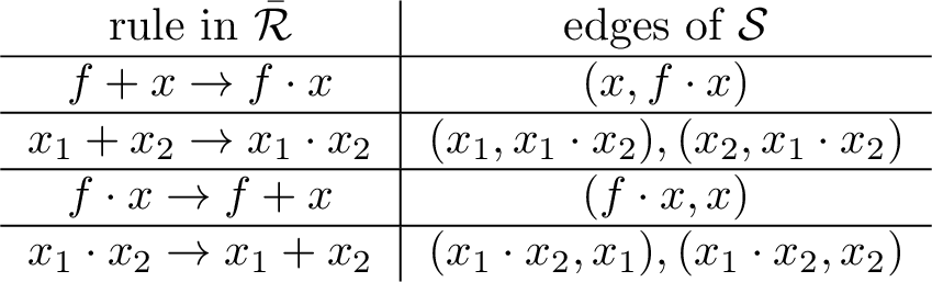
We fix here an alphabet \({\cal A}= \{A,B,C\}\), an external molecule set \({\cal F}=\{BC\}\) with only one element, a standard deviation \(\lambda=1\), \(m_{ref}=\log_{10}(k_{min}/k_{ref}) = 2\), and a maximum level \[n_{max}= \max\{|x|, x\in \bar{\cal R}\} = 5,\] see Fig. 3 , and \(n_{max}=7\), see Fig. 4 (up to 6 or 8 atoms), while letting the \(\sigma\)-parameter, see eq. (1.3), take 20 values between 0.2 and 0.9. Results for \(n_{max}=7\) look very similar to those for \(n_{max}=7\), except that they are less noisy, and it took about 1 hour instead of a few minutes to generate the data.
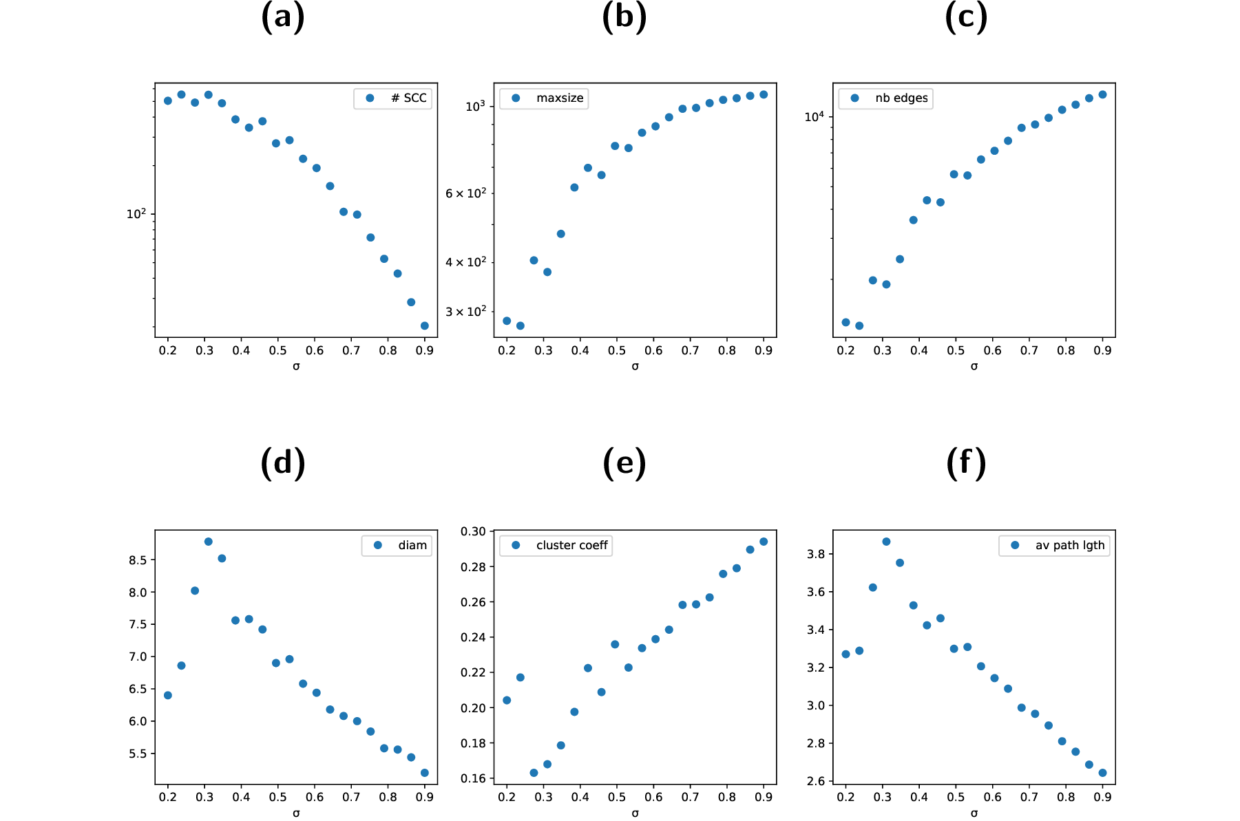
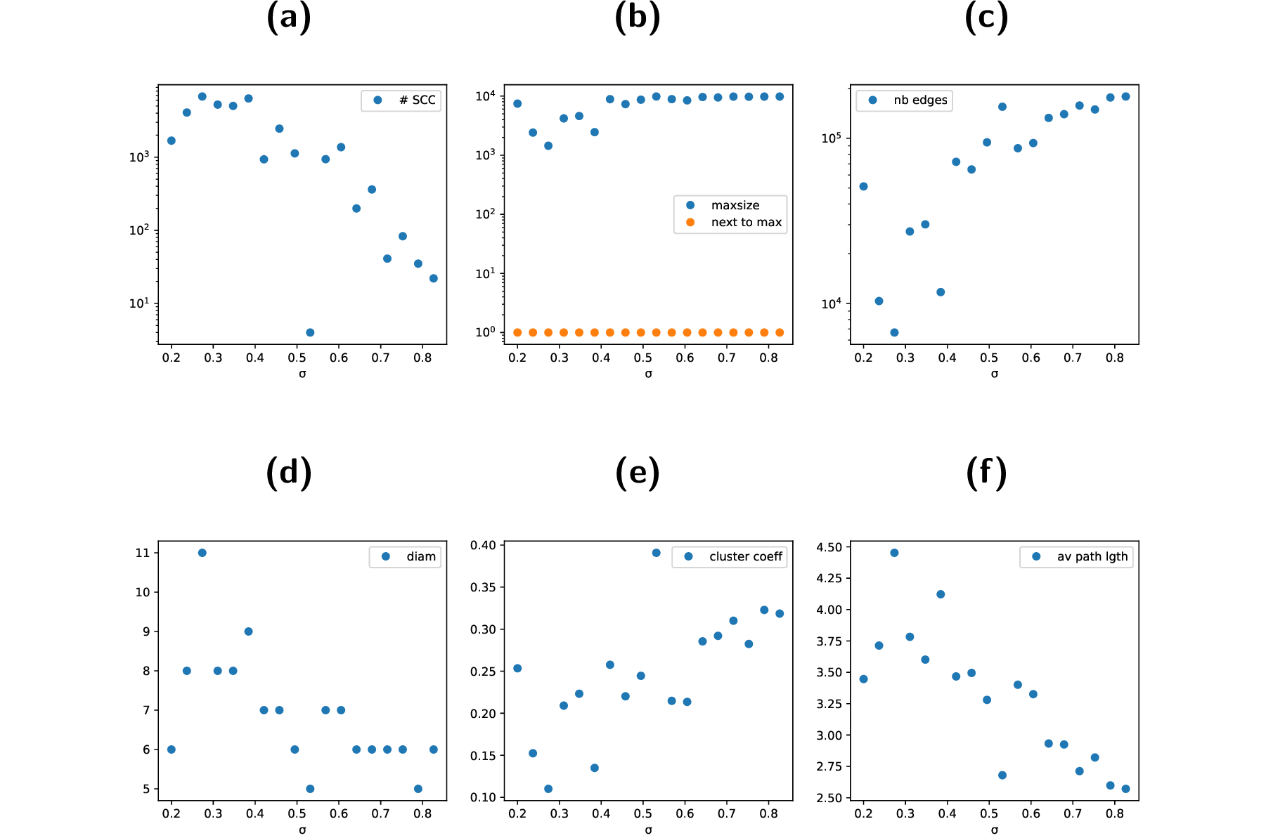
Fig. 3 (a), (b), (c) shows the number of SCCs, size \(N(\sigma)\) (number of molecules) and number of edges \(E(\sigma)\) of the largest strongly connected component (SCC) of the substrate graph, average over a sample of 50 graphs. Plot (b) also shows the size of the next-to-largest SCC, which is 1. Unsurprisingly, both increase with \(\sigma\), because the acceptance probability of any rule also does. It saturates at \(1092 = 3+3^2 + \cdots + 3^6\) for \(\sigma\) large enough, implying that all molecules of level \(\le 5\) are in the same SCC. On the other hand, \(E(\sigma)\), while large, does clearly not scale like \(N(\sigma)^2\), which means that the graph is very sparse. Comparison to results for \(n_{max}=7\), see Fig. 4, suggests that \(E(\sigma)\propto N(\sigma)\) instead, with a prefactor \(\sim 10\); due to time limitations, we considered only one graph, which explains why data look noisy (all the more sore as \(\sigma\) is small, since then only few primitive reactions are actually contributing). Note that (contrary to the case of Erdös-Rényi graphs), no phase transition is discernible.
Then Fig. 3 (d), (e), (f) reports other quantities related to the largest SCC: its diameter \(D(\sigma)\) (maximum eccentricity), which is the largest graph distance (= shortest path length) between two nodes; the clustering coefficient \(0<C(\sigma)<1\); and its characteristic (average) path length (average graph distance between two nodes), \(L(\sigma)\). The fact that \(C\) remains bounded below, and \(L\) remains bounded from above by some small number, fits the small world paradigm. As \(\sigma\) increases, the diameter decreases (despite the size increase), and so does the characteristic path length, because there appear shortcuts; at the same time, the clustering coefficient increases.
2.2 Out-of-equilibrium simulations: dynamical features↩︎
Next, we kept the equilibrium assumption for anabolic rules, but dropped it for catabolic rules, turning them into irreversible reactions, either \(x_1\cdot x_2\to x_1 + x_2\) or \(x_1 + x_2\to x_1\cdot x_2\). The direction was chosen by favoring networks featuring a pair of coupled autocatalytic cycles. Namely, such networks exhibit multistationarity in some regimes; see §2.2.1 for such an example of rule-based network. RRBCN networks are randomly generated rule-based networks, so that the network in §2.2.1 is an instance of RRBCN network. §2.2.2 goes on prove that similar coupling structures between autocatalytic cycles are very common in RRBCN models, fostering the appearance of multiple stationary states.
2.2.1 A pair of coupled autocatalytic cycles↩︎
The inspiration comes from a network with a pair of coupled autocatalytic cycles which we now discuss. It is based on the following mechanisms (primitive rules) on a two-letter alphabet \({\cal A} = \{A,N\}\) with external molecule set \({\cal F} = \{A,NA\}\); for more readability, we use lower indices for repeated letters, e.g. \(NA_4 N\) instead of \(NAAAAN\):
(anabolism) \(A+ A_2 \underset{\bar{k}_0}{\overset{k_0}{\rightleftarrows}} A_3, \qquad NA + A_3 N \underset{\bar{n}_0}{\overset{n_0}{\rightleftarrows}} NA_4N;\)
(catabolism) \(A_4 \overset{\bar{k}_1}{\to} A_2 + A_2, \;\;NA_4N \overset{\bar{n}_1}{\to} NA_2 + NA_2,\;\; A_2N + A_3 \overset{\kappa_1}{\to} A_2NA_3, \;\;A_2NA_3\overset{\kappa_2}{\to} A_2 + NA_3\).
The network \(\bar{\cal R}(n_{max})\) is the network obtained from these rules by completion, with cut-off at level \(n_{max}\). It contains two autocatalytic cycles, denoted \({\cal C}_A\) and \({\cal C}_N\), both of the same type as the core formose reaction network; the autocatalytic cycle \({\cal C}_A\) for \(n_{max}=3\), resp. \({\cal C}_N\) for \(n_{max}=5\) takes the form \(\{A_2 \overset{+A}{\rightleftarrows} A_3 \overset{+A}{\rightleftarrows} A_4 \to 2A_2\}\), resp. \(\{NA_2 \overset{+A}{\rightleftarrows} NA_3 \overset{+AN}{\rightleftarrows} NA_4N \to 2NA_2\}\). The autocatalytic cycle \({\cal C}_A\) in \(\bar{\cal R}(n_{max}=5)\) is extended to a cycle extending to species \(A_5,A_6\); see e.g. [30] for a visualization of a real-world formose network. Whatever the cut-off level, these cycles are known to be autocatalytic, so that compositions of the type \(([A] = 1, [a] = \varepsilon)\), resp. \(([A]=[NA]=1, [n]=\varepsilon)\) where \(a\), resp. \(n\) is one of the species of \({\cal C}_A\), resp. \({\cal C}_N\), and \(\varepsilon\ll 1\), are unstable, with the concentrations of all species in \({\cal C}_A\), resp. \({\cal C}_N\) growing exponentially with time. We control the concentration of external molecules by a CSTR (continuously stirred chemical reactor) formalism, see e.g. [36] : \(A\), resp. \(NA\), is chemostatted via a high injection rate \(i_A\), resp. \(i_{NA}\), and degradated through a dilution rate \(\delta_A\), resp. \(\delta_{NA}\), yielding equilibrium concentrations \[[A]_{eq} = i_A/\delta_A, \qquad [NA]_{eq} = i_{NA}/\delta_{NA}.\] This ensures that concentrations of species within cycles saturate at a high level instead of growing indefinitely. Since species in \({\cal C}_A\) and \({\cal C}_N\) are disjoint, this defines two stable stationary states with compositions \([\cdot]_A\), resp. \([\cdot]_N\), with \(([a]_A >0, [n]_A=0)\), resp. \(([a]_N = 0, [n]_N>0)\) for any species \(a\), resp. \(n\) in \({\cal C}_A\), resp. \({\cal C}_N\).
The coupling of the two cycles via the rules \(A_2 N + A_3 \overset{\kappa_1}{\to} A_2NA_3 \overset{\kappa_2}{\to} A_2 + NA_3\) defines a ‘cross-over’ type sequence of reactions: one \(A\) atom is exchanged between the two reactants. (The two cycles can be realized by taking the glyoxylate cycle for \({\cal C}_A\), and a nitrogenated version for \({\cal C}_N\). Addition reactions are aldolizations, and the ‘cross-over’ is then a transamination. The actual chemical network contains a few more intermediates).
We present two sets of numerical simulations obtained using Julia’s Catalyst and HomotopyContinuation libraries for chemical networks, which allow an easy input for reactions, and a calculation of all stationary states:
one for the restricted \({\cal C}_A(n_{max}=3)\) cycle coupled to \({\cal C}_N(n_{max}=5)\);
the other for the unrestricted \(\bar{\cal R}(n_{max}=5)\) network, coupling \({\cal C}_A(n_{max}=5)\) with \({\cal C}_N(n_{max}=5)\).
Parameter choices are specified in Suppl. Info. §I.C. Anabolic rules in case 1. have been made irreversible, and rates of other reactions are in a close range. In case 2., anabolic rules are reversible and detail-balanced with flat thermodynamic balance \(\Delta G^0=0\), but rates are scattered over 8 ranges (from \(\varepsilon^{-3}\) to \(\varepsilon^5\), with \(\varepsilon= 1/4\)). Dynamical simulations are presented in case 1. (see Fig. 5, 6) which start from the equilibrium values for \([A], [NA]\), and high values for \({\cal C}_A\) species/very low values for \({\cal C}_N\) species or vice-versa, corresponding to possible invasion of \({\cal C}_A\) by \({\cal C}_N\) species or vice-versa. Simulations show that invasions fail: for instance, \({\cal C}_N\) species disappear in the first case, while \({\cal C}_A\) species concentrations converge to their stationary values. In short, single-cycle stationary states with compositions \([\cdot]_A\), \([\cdot]_N\) are stable.
In both cases 1. and 2., one gets 4 stationary states, see Fig. 7 and 8:
the two exclusive (single-cycle) stationary states with compositions \([\cdot]_A\), \([\cdot]_N\), which are stable; plus two unstable states:
the trivial equilibrium state with \([A]=[A]_{eq},\, [NA] = [NA]_{eq}\) and all other concentrations vanishing;
and a cooperative state \([\cdot]_{A,N}\) (all A-cycle and N-cycle species present).
The cooperative state was proved to be unstable by checking that the Jacobian matrix of the system at \([\cdot]_{A,N}\) has a positive eigenvalue; numerical simulations are a good illustration.
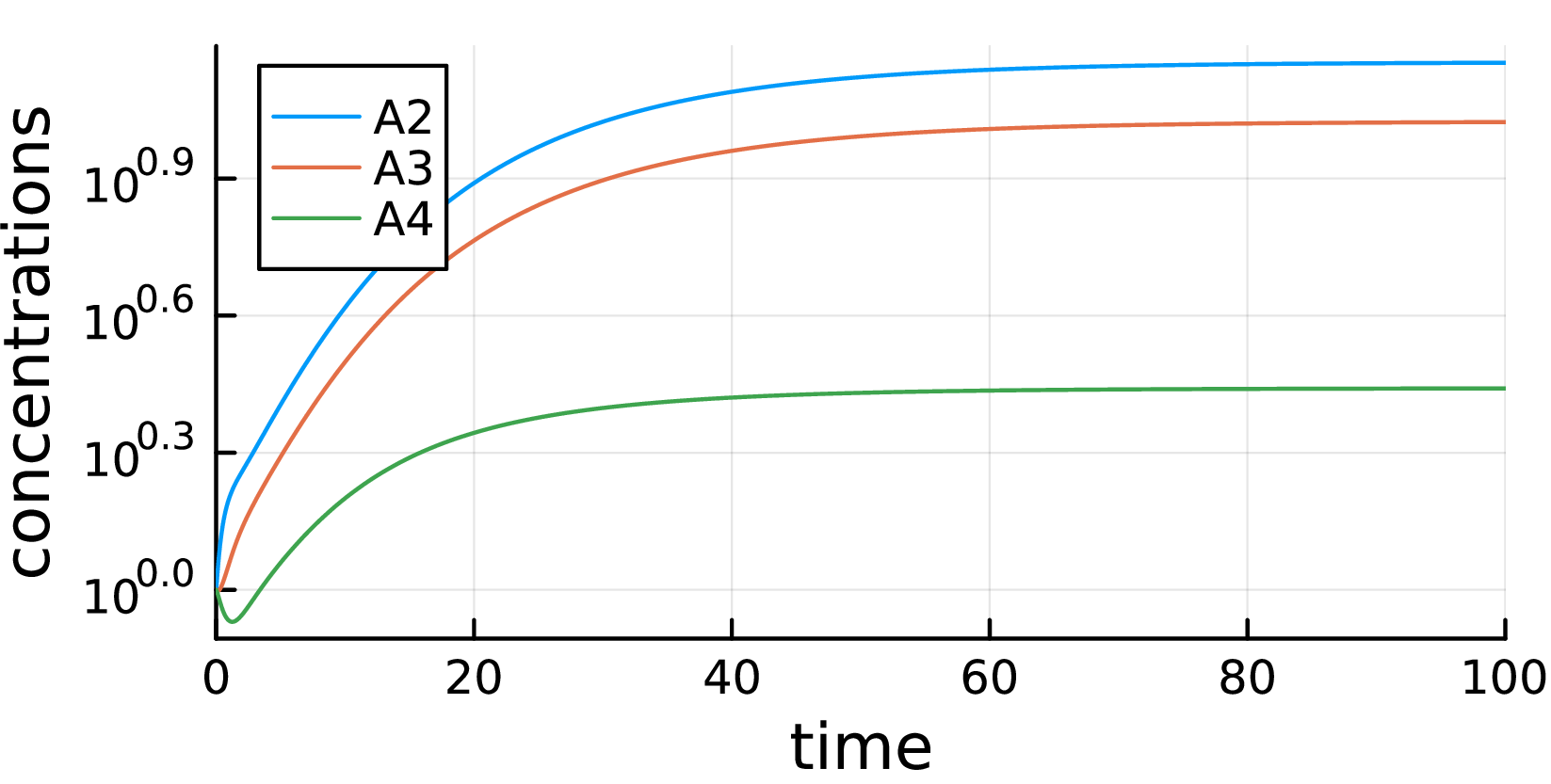
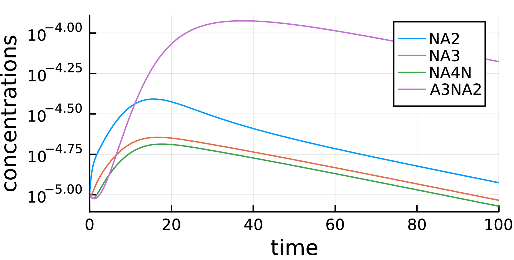
Figure 5: 2-cycle coupled network started from a neighborhood of the A-cycle. a — Total graph, b — Connection graph
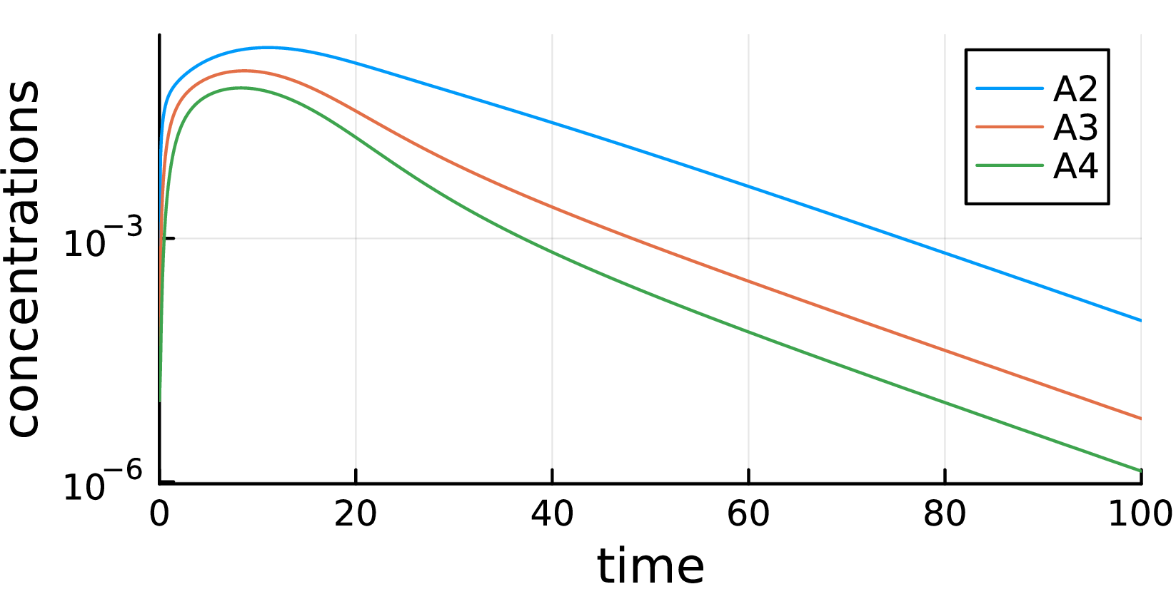
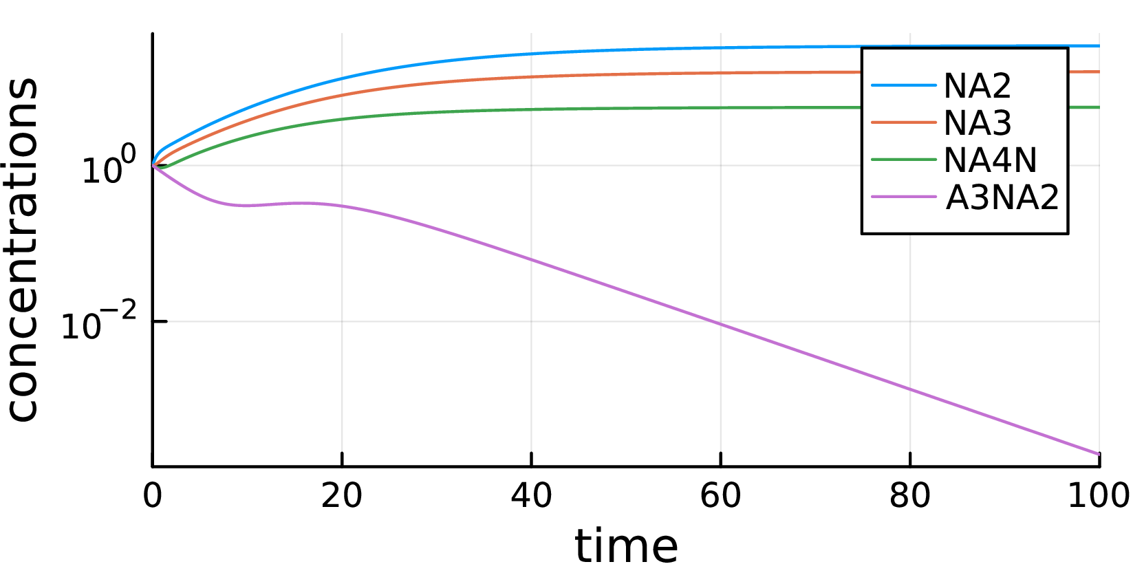
Figure 6: 2-cycle coupled network started from a neighborhood of the AN-cycle. a — An autocatalytic SCC, b — Another autocatalytic SCC
cm
![Figure 7: Stationary states for {\cal C}_A(n_{max}=3) coupled to {\cal C}_N(n_{max}=5). From left to right and top to bottom: [\cdot]_{eq}, [\cdot]_A, [\cdot]_N, [\cdot]_{A,N}.](/article/2502.11692/2_cycle_SS35.png "fig:")
![Figure 8: Stationary states for {\cal C}_A(n_{max}=5) coupled to {\cal A}_N(n_{max}=5). From left to right and top to bottom: [\cdot]_{N}, [\cdot]_{A,N}, [\cdot]_{eq}, [\cdot]_{A}.](/article/2502.11692/2_cycle_SS55.png "fig:")
One can check that exclusive stationary states survive and remain stable when \(\kappa_2\) is decreased down to \(0\). Thus the general message is: two autocatalytic cycles, coupled by some reverse catabolic reaction \(x_1+x_2\to x_1\cdot x_2\), with \(x_1\) lying in one cycle, \(x_2\) in the other, can produce stable exclusive stationary states. This generalizes in principle to multiple arrays of autocatalytic SCCs \(\{C_i\}_{i=1,2,\cdots}\) coupled by catabolic rules \(x_I + x_j \to x_i\cdot x_j\) defining an undirected graph ConnG with nodes \(\{1,2,\cdots\}\) and edges \(\{(i,j)\;|\, x_i + x_j \to x_i\cdot x_j\}\). Thus one expects to get a set of stable stationary states indexed by independent sets of ConnG (i.e. maximal subsets of ConnG satisfying hard-core exclusion along edges) as in [37]. We show in the next paragraph how to generate such arrays in the RRBCN framework.
2.2.2 Autocatalytic cycles and multistationarity in RRBCN models↩︎
Instead of picking a multistationary network, we perform here an automatized search for pairwise coupled autocatalytic cycles in RRBCN models. It turns out that this is a very common feature if the parameters of the models are well-chosen. The favorable parameter range is difficult to assess a priori. We took here simply \(p=q\) following (4 , ?? ), and chose to make all anabolic rules reversible. It helped for numerics that we picked \(z=1\) (Model I) and \(p=q=0.88\) high (see Suppl. Info. §I.D.), so that the number of rules is high even though the truncation level \(n_{max}=5\) is low. We made simulations for two and three atom types; the results are similar, but graphs are much larger for \(|{\cal A}|=3\), so that they cannot be drawn properly with the Python networkx package. Hence we kept to \({\cal A}=\{a,n\}\) as before, with lower-case letters this time for convenience. The foodset here is \({\cal F} = \{a,n,na,an\}\) (\(na\)-additions are different from \(an\)-additions because anabolic reactions are systematically written in the form \(f+x\to f\cdot x\)). Corresponding edges in the \({\cal S}\)-graph are drawn red/blue/green/magenta if \(f=a/n/na/an\). Edges coming from catabolic rules are black.
All anabolic rules were chosen reversible. We assumed for the network generation that catabolic reactions were irreversible (see Suppl. Info. §I.D.). This amounts to neglecting reactions of the form \(x_1 + x_2 \to x_1\cdot x_2\) which are of kinetic order 2. Assuming further that foodset molecules \(f\) are chemostated, we are in the "dilute" framework studied in [35], where the generator of the dynamics is linear, and a connectivity analysis of the substrate graph \(\cal S\) is enough to detect autocatalysis. Namely, let \({\cal C}_i, i=1,2,\ldots\) be the strongly connected components (SCCs) of \(\cal S\). Consider among the \({\cal C}_i\) those such that there exists a catabolic reaction \(x_1\cdot x_2\to x_1 + x_2\) with all three species \(x_1\cdot x_2, x_1, x_2\) in \({\cal C}_i\). Then (if the rates of rules exiting \({\cal C}_i\), i.e. with the reactant \(x\) in \({\cal C}_i\) and at least one product outside, including dilution \(x\to \emptyset\), are small enough), any trace of any species in \({\cal C}_i\) implies exponential growth of all species in \({\cal C}_i\), which means that the network restricted to \({\cal C}_i\) is autocatalytic. We simply call autocatalytic SCCs those \({\cal C}_i\) that satisfy the above topological property.
Next, we consider the couplings between the autocatalytic SCCs. The conclusion of §2.2.1 suggests that we look for sequences of reverse catabolic reactions coupling \({\cal C}_i\) and \({\cal C}_j\) \((i\not=j)\). We proceed as follows. Index all SCCs (autocatalytic or not) by integer numbers; we first define a coarse-grained directed graph G_fork on the set of SCC indices. Take any catabolic rule \(x\cdot y \rightleftarrows x + y\), and orient it in the reverse direction \(x+y\to x\cdot y\). If \((x, x\cdot y)\) are in SCCs indexed by \((i,j)\), \(i\not=j\), draw an edge \(i\to j\); similarly for the pair \((y,x\cdot y)\). Then we build the undirected graph ConnG with:
node set equal to the set of indices of autocatalytic SCCs;
edge set equal to the set of pairs \((i,j)\) of nodes of ConnG such that there exists a SCC \(k\) (not necessarily autocatalytic) reachable both from \(i\) and from \(j\) by a directed path in G_fork.
A particular case is when there exists a catabolic reaction \(x+y\to x\cdot y\) with \(x\in {\cal C}_i, y\in {\cal C}_j\), \(x\cdot y\in {\cal C}_k\), \(i\not=j\not=k\), and \(i,j \in\) ConnG: then G_fork contains the edges \((i,k),(j,k)\), so that \((i,j)\) are connected by an edge in ConnG.
We generated ten instances of random networks with \(n_{max}=5\). Two of them (resp. 5, 3) contained one (resp. 2, 3) autocatalytic SCC (generating more instances shows that it is quite possible to get none). Fig. 9 reports one instance with 3 autocatalytic SCCs indexed 0, 3, 5, see plot (a) for the substrate graph \(\cal S\). SCC #5 is somewhat large (see plot (b)) and would require a larger plot, but SCCs #0 and #3 are small components, exhibiting 3, resp. 4 different addition mechanisms (see plots (c) and (d)). All 3 components are connected by ConnG (plot (e)); in all ten instances, \(\textsf{ConnG}\) is the total graph. Plot (f) gives a streamlined plot of their location within \({\cal S}\), with \({\cal C}_0\) (resp. \({\cal C}_3\)) nodes and edges colored red (resp. blue).


Figure 9: Autocatalytic SCCs and their pairings. a — Total graph, b — An autocatalytic SCC, c — Another autocatalytic SCC, d — Yet another autocatalytic SCC, e — Connection graph ConnG, f — Pairing btw autocatalytic SCCs #0 and #3
3 Explorations of high-level mechanisms: theory and simulations↩︎
By contrast with §2, we explore in this section the high-level random reactivity structure of RRBCN models. This structure is determined by the number and organization of high-level mechanisms (equivalently, complex primitive rules). Among the foremost questions, formulated already in the introduction: are there arbitrarily complex mechanisms, suggesting possible open-ended evolution ? if not, what are the most complex mechanisms ? how complex is a ‘typical’ mechanism ? what is the typical shape of a large-level reaction subnetwork ?
Simulations are of limited value for such questions. The main tool here has been an approximate mapping to models of random tree growth, called Galton-Watson models, which are classical in the mathematics literature (§3.1). This mapping has made it possible to delve into the above questions. We report here mainly on asymptotic rule statistics (§3.2 for Model I, §3.3 for Model II) which answer the above questions regarding the complexity of mechanisms within the limits of RRBCN models. Models I and II behave very differently in this respect: whereas the complexity of mechanisms is capped in Model I, there are regimes in the parameter space of Model II for which one finds arbitrarily complex mechanisms. Regimes present themselves in the form of a phase diagram. This fundamental distinction explains why it has been possible to validate our predictions for Model I by detailed simulations, while (despite no contradiction) numerical evidence is more elusive for Model II.
A large part of our work has been relegated to Suppl. Info., §II-V, notably simulations (§V), with only main arguments and plots presented in Main Text. Also, work in progress on the typical shape of a large-level reaction subnetwork is presented in Suppl. Info. §III.B. (anabolism) and IV.B. (catabolism); superposing the anabolic and catabolic parts to study the typical shape of reaction subnetworks is a non-trivial, yet unsolved problem, left for further investigation.
3.1 Mapping to tree models↩︎
As pointed out earlier, parameter values \(p\simeq 1\) or \(z\simeq 0\) make the large-level random structure very poor. This suggests we look at intermediate regimes where \(p\) is not close to 1 (typically, \(p<0.5\); possibly, \(p\to 0\)) and \(z\) is not too small (typically, \(z>0.5\)). These conditions favor the emergence of a small number of unexpectedly complex mechanisms \(\rho\) (with \(m_{\rho}\ge 10\), say), an interesting scenario for evolution. They also make simulation tools less practical, or sometimes prohibitively time- and memory-consuming (the program crashes), because the number of molecules, roughly \(|{\cal A}|^{n+1}/2\), increases exponentially with level \(n\). Limiting to exhaustion of primitive rules (see 1.4) is necessary, but not sufficient when the number of those becomes large.
Fortunately, many large-level observables of RRBCN models may be computed analytically through an approximately mapping to a random tree model, that we set out to describe. Anabolism and catabolism can be studied separately and with similar techniques. We deal here with anabolism, fix \(f\in {\cal F}\) and consider admissible reactions \(\rho : f+x\to f\cdot x\). Context completion here is bilateral for a better general agreement with real-world chemistry: if \(f\) reacts with \(x\), then it reacts with \(r_1\cdot x\cdot r_2\) (and the product is branching if \(r_1\) is not trivial). In particular, it reacts with \(x\cdot r_2\). Representing the set of all molecules \(x=A_1 A_2\cdots\) as a tree, see Fig. 10 for \({\cal A} = \{A,B,C\}\), keeping only those \(x\) that do not react with \(f\) (in red), and those such that \(\rho\) is a primitive rule (in blue), yields a composition tree. By construction, a composition tree is a tree \({\mathbb{T}}={\mathbb{T}}(f)\) with (formal) root \(\emptyset\), red inner vertices and blue leaves. The maximal composition tree (containing all words, in red) is obtained when \(f\) does not react with any \(x\).
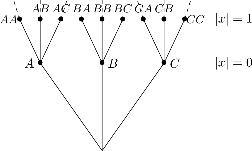
Equivalently, letting \(\omega_x^f\) be the decision variable attached to the rule \(f+x\to f\cdot x\): \[(x\in {\mathbb{T}}(f)) \Leftrightarrow \Big(\forall x'\subsetneq x, \omega^f_{x'} = 0\Big) \label{eq:xTf}\tag{6}\] and \(x\in {\mathbb{T}}(f)\) is a leaf iff \(\omega^f_x=1\). See Suppl. Info. §IV. A. for a similar construction applied to catabolism in terms of fragmentation tress.
Our predictions, consistent with available (partial but still very substantial) simulations, are built on an approximate mapping from our model to an inhomogeneous Galton-Watson (GW) tree model. We refer the reader to the book [38], Chapter 1 & 5 for a standard introduction to the subject. GW trees are also used to represent the different generations of cellular division models in biology [39]. By definition, individuals are indexed by an integer generation number. Each generation \(n\) individual \((n,j)\) has a random number of descendants \(\zeta_{(n,j)}\) according to a fixed progeny law; the model is called inhomogeneous if that law depends on \(n\). All progenies \(\zeta_{(n,j)}\) are assumed to be independent. Moments of the model may be computed using generating functions \(f_n(s) = {\mathbb{E}}[s^{\zeta_n}]\), \(s\ge 0\), where \(\zeta_n\) is any of the \(\zeta_{(n,j)}\) variables.
Our mapping is based on a \((1/|{\cal A}|)\) expansion for \(|{\cal A}|\) large. We denote by \({\cal X}_n\) the set of level \(n\) words, and call (primitive) \(f\)-reactants those \(x\) such that \(\rho : f+x\to f\cdot x\) is a (primitive) rule. We observe the following:
Let \(x=A_1\cdots A_n\in {\cal X}_{n-1}\), and \(A\in {\cal A}\). Assume \(x\in {\mathbb{T}}(f)\). Then \(x\cdot A\in {\mathbb{T}}(f)\) if and only if for all \(k=0,\ldots,n\), \(A_{n-k+1}\ldots A_n\cdot A\) is not a primitive \(f\)-reactant. (By abuse of notation, we let \(A_{n-k+1}\ldots A_n \cdot A = A\) if \(k=0\)). Namely, as already observed, all other subwords of \(x\cdot A\) are actually subwords of \(w\), therefore are not \(f\)-reactants since \(x\in {\mathbb{T}}(f)\).
Choose \(w=A_1\cdots A_n\) uniformly in \[V_{n-1}({\mathbb{T}}) = \{x\in {\mathbb{T}}\;|\;|x|=n-1\}.\] Denote \(\zeta_x = (\zeta_x^A)_{a\in {\cal G}}\) its progeny; in other words, \(\zeta_x^A=1\) iff \(x\cdot A\in {\mathbb{T}}\). Then, to leading order in \(1/|{\cal A}|\), the progeny law of \(x\) has independent components, and the law of each component is independent of the choice of \(x\). Namely, the \((n+1)\times|{\cal A}|\) variables \[\omega^f_k(x,A) \equiv \omega^f_{A_{n-k+1}\ldots A_n\cdot A}, \qquad 0\le k\le n, \; A\in {\cal A}\] (see §6 ) are independent since they are indexed by different words. Furthermore, \(\omega^f_{A_{n-k+1}\ldots A_n\cdot A}\) depends on \(w\) only through the possibility that \(A_{n-k+1}\ldots A_n\cdot A\) is a subword of \(w\). However, fixing these \(k+1\) atoms implies restraining to a proportion \(\approx |{\cal A}|^{-(k+1)}\) of \(V_n({\mathbb{T}})\). For \(n=O( |{\cal A}|/p)\), this implies (considering all potential \(n-k\) locations of \(A_{n-k+1}\ldots A_n\cdot A\) in \(w\), and taking into account the variance \(p(1-p)\) of a Bernoulli law) a correcting term to the progeny of order \(p(1-p)\times |{\cal A}|^{-(k+1)} \times n = O(|{\cal A}|^{-1})\), except for \(k=0\). The correction associated to the \((k=0)\) term can be computed, and – as turns out – does not alter significantly the consequences of the above observations.
The mapping to a GW model resulting from these key observations is described in §3.2 for Model I, and §3.3 for Model II. The approximate mapping makes statistical quantities for the large-level random reactivity structure of RRBCN models analytically computable. We present the results in the Main Text, and refer the reader to Suppl. Info. for proofs.
The mapping turns exact when \(|{\cal A}|\to\infty\). This makes it particularly well-suited for applications to chemistry involving some coarse-graining, since \(\cal A\) should span a set of functional groups of size 20-30 at least. Actually, simulations show a surprisingly good agreement with our estimates in the case of Model I (see Suppl. Info. §V.A. and §V.C.) even when \(|{\cal A}|=3\), describing e.g. heavy atoms for CHON molecules.
3.2 Asymptotic rule statistics: the case of Model I↩︎
We discuss here the structure of large-level anabolic primitive rules for Model I, as deduced from asymptotics for anabolic composition trees (§3.2.1). Details and proofs may be found in Suppl. Info. §II. Results for catabolis are briefly discussed in §3.2.2, see Suppl. Info §IV.
3.2.1 Anabolism↩︎
In the whole paragraph, we fix a composition tree \({\mathbb{T}}={\mathbb{T}}(f)\). Dealing simultaneously with several foodset molecules is a very easy generalization; see next section (Model II), where we start directly from a general foodset \(\cal F\).
Taking into account the two Key observations, and forgetting \((k=0)\) corrections, one can expect that, for generic \(w\in V_{n-1}({\mathbb{T}})\), \(w.A\in V_{n}({\mathbb{T}})\) with probability \(\sim {\mathbb{P}}[\omega^f_k(x,A)=0, \;1\le k\le n] = (1-p)^n\). Thus, the mapping of Model I is to the inhomogeneous GW model with generation \(n\) progeny law equal to the binomial law \[(progeny\;law\;of\;GW\;model) \qquad Bin(|{\cal A}|,(1-p)^n)\]
In more concrete terms, the average number of descendants of a typical vertex of level \(n-1\) in a composition tree is roughly \(\sim |{\cal A}| (1-p)^n.\) This is to be understood in a weak sense (see below), namely, \(\log \langle |V_n({\mathbb{T}})|\rangle \sim \log \prod_{k=1}^{n} (|{\cal A}|(1-p)^k)\) for \(n\) large enough but still less than \(O(|{\cal A}|/p)\), or \[\log \langle |V_n({\mathbb{T}})|\rangle \sim n \Big( \log |{\cal A}| - \frac{n+1}{2} \log(1/(1-p)) \Big) . \label{eq:I-logVn}\tag{7}\]
Thus composition trees dwindle rapidly, and become rapidly extinct as \(n\) exceeds the value of \(n\) which maximizes (7 ), \[{\mathrm{(maximum\;average\;size\;level) }} \qquad n_0:= \frac{\log(|{\cal A}|)}{\log(1/(1-p))}, \label{eq:n0}\tag{8}\] solution of the equation \[(1-p)^{n_0} |{\cal A}| = 1.\] In practice, since we are interested in small values of \(p\), we often use the approximate value \[n_0\sim \frac{\log(|{\cal A}|)}{p}.\] Note that the r.-h.s. in (7 ) becomes negative when \(n>n'_0\), with \[{\mathrm{(extinction\;level)}} \qquad n'_0:= 2n_0 \label{eq:n390}\tag{9}\]
The actual interest is not in the composition tree, but in its leaves, which are the primitive \(f\)-reactants. We characterize the set of leaves \[{\mathrm{Prim}} = \cup_{n\ge 0} {\mathrm{Prim}}_n, \qquad {\mathrm{Prim}}_n = {\mathrm{Prim}} \cap V_n({\mathbb{T}}) \label{eq:Prim95n}\tag{10}\] by its shape: size (number of primitive rules) by level, and top level, which is the maximum complexity index of all \(f\)-addition mechanisms.
(see Suppl. Info., §II.A. and §II.B.). Let \(x\in V_{n-1}({\mathbb{T}})\). Recall (see Key observation 2) that \(f+x\cdot A\to f\cdot x\cdot A\) is a primitive reaction iff \(\omega^f_k(x,A) = 0\), \(1\le k\le n-1\), and \(\omega^f_n(x,A) \equiv \omega^f_{A_1\cdots A_n\cdot A } = 1\). Thus the number of blue vertices of level \(n\) may be computed as above, except that the last generation progeny law is not Bin\((|{\cal A}|,p_n)\) but Bin\((|{\cal A}|,p(1-p)^{n-1})\). Taking into account the constant prefactor \(|{\cal A}|(1-p)^{|{\cal A}|}\) coming from the \((k=0)\) correction (see Suppl. Info §II.B.), this implies: \[\begin{align} \langle |\mathrm{Prim}_n|\rangle &\approx & |{\cal A}| (1-p)^{|{\cal A}|} \, \times \prod_{k=1}^{n-1} (|{\cal A}| (1-p)^k) \nonumber\\ && \qquad \qquad \times (|{\cal A}| p(1-p)^{n-1}) \nonumber\\ &=& p |{\cal A}|^{n+1} (1-p)^{|{\cal A}|-1 + n(n+1)/2} \label{eq:Primn} \end{align}\tag{11}\] Just like \(\langle V_n({\mathbb{T}})\rangle\), it is maximum for \(n\simeq n_0\), see (8 ), which can therefore be thought as the ‘typical’ complexity of a specific anabolic mechanism. Figure 11 gives the number of primitive rules in terms of \(n\) for various values of \(p\).

The average total number of primitive reactions is \(\langle |\mathrm{Prim}| \rangle= \sum_{n\ge 0} \langle|\mathrm{Prim}_n|\rangle\). The largest term in the summand is obtained for \(n\simeq n_0\), yielding \(\langle |\mathrm{Prim}|\rangle \approx p|{\cal A}|^{n_0+1} (1-p)^{|{\cal A}|-1 + n_0(n_0+1)/2} \sim p |{\cal A}|^{1+ \log|{\cal A}|/2p}.\)
(see Suppl. Info., §II.C. and §II.D.). The top level (or height of \({\mathbb{T}}\), denoted ht\(({\mathbb{T}})\)) is the level at which the tree \({\mathbb{T}}\) becomes extinct. Let \((Z_n)_{n\ge 0}\) be the number of generation \(n\) individuals in the GW model. Denote by \(P(m,j;n,i):={\mathbb{P}}[Z_n =i \;|\;Z_m =j ]\) \((n>m)\) the inhomogeneous iterated kernel associated to the Markov process \((Z_n)_{n\ge 0}\). By definition, \({\mathbb{T}}\) is extinct at time \(n\) with probability \(u_{0,n}:=P(0,1;n,0)\). The Chapman-Kolmogorov equation implies \(u_{0,n} = \sum_{k\ge 0} P(0,1;1,k) P(1,k;n-1,0)\); then \(P(1,k;n-1,0) = (P(1,1;n-1,0))^k\) by independence of the branches. Denote by \(u_{k,n} := P(k,1;n,0)\) the probability to be extinct at time \(n\) starting from one individual at time \(k\); then we have found \(u_{0,n} = f_1(u_{1,n})\). Note that \(u_{n-1,n} = (1-p_n)^{|{\cal A}|} = f_n(0)\). Iterating, we get \(u_{0,n} = f^{(n-1)}(u_{n-1,n}) = f^{(n)}(0)\); thus, \[u_{0,n} = f^{(n-1)}((1-p_n)^{|{\cal A}|}). \label{eq:u0n}\tag{12}\]
Extinction probabilities are estimated as a by-product of a general estimation for the iterated function \(f^{(n)}(s), 0<s<1\), see Suppl. Info. §II. B., where it is proves that trees grow extinct with high probability at a level \(\sim 2n_0\). Thus the top level (maximum mechanism complexity) is roughly equal to the extinction level \(n'_0\) of eq. (9 ).
(see Suppl. Info., §II.E.). One may be interested in measuring and estimating \(\langle \log |V_n({\mathbb{T}})| \rangle\) instead of \(\log \langle |V_n({\mathbb{T}})|\rangle\), and \(\langle \log (|\mathrm{Prim}_n|)\rangle\) instead of \(\log \langle |\mathrm{Prim}_n|\rangle\). This induces in general a supplementary prefactor \(<1\), since (by convexity) \(\langle \log(X)\rangle \le \log \langle X\rangle\) for any positive random variable \(X\). This is a well-known issue in the study of disordered media; interpreting \(|V_n({\mathbb{T}})|\) as a random partition function, \(\langle \log |V_n({\mathbb{T}})| \rangle \sim \log \langle |V_n({\mathbb{T}})|\rangle\) for large \(n\) is indicative of a self-averaging measure, i.e. the distribution of \(|V_n({\mathbb{T}})|\) is very concentrated. True asymptotics \(n\to\infty\) are however irrelevant here, since trees go extinct.
It is proved in Suppl. Info., §II. C., that self-averaging holds for the Galton-Watson model, but not for our original model.
3.2.2 Catabolism↩︎
We only sketch our results, and refer the reader to Suppl. Info. §IV.A. for more information. Instead of a set of \(f\)-dependent composition trees \({\mathbb{T}}(f)\), we get a unique fragmentation tree \({\mathbb{T}}_{frag}\), whose leaves coincide with the set of \(x\) such that \(x\) is decomposable by a primitive rule, i.e. at least one catabolic reaction of the form \(x\to x_1+ x_2\) (\(x_1\cdot x_2= x\)) is a primitive rule of the RRBCN-network \(\bar{\cal R}\). Then maximum average size level \(n_0\) (8 ), resp. extinction level \(n'_0\) (9 ) have equivalent counterparts \(n_{frag}\), resp. \(n'_{frag}\) for catabolism, see Suppl. Info., eq. (IV.6), \[n_{frag} \sim \sqrt{\frac{2\log|{\cal A|}}{q}}, \qquad n'_{frag}\sim \sqrt{3}\;n_{frag}\] Multiple fragmentation processes a priori available for any given \(x\) explain why the complexity of catabolic mechanisms is typically much lower than in the anabolic case, as evidenced by the square-root in \(n_{frag}\).
3.3 Asymptotic rule statistics : the case of Model II↩︎
We now deal with Model II by reusing the same techniques. The analysis is more involved than for Model I. Our main finding is a phase diagram in the parameter set \((p, q, z, |{\cal A}|, |{\cal F}|)\) for the structure of large-scale primitive rules, see Fig. 12, including a phase in which the number of primitive rules is infinite, which hints at the eventuality for open-ended evolution. We discuss the case of anabolism in some detail, but refer to Suppl. Info. §III for complements and proofs. The case of catabolism, which is similar, is left out entirely, see Suppl. Info. §IV.A, in particular, the catabolic phase diagram, Fig. IV. 13.
The fugacity parameter \(z\) is crucial here. In particular, for \(z\) not too large, the composition tree is infinite; more precisely, the average fraction of molecules of level \(n\) that react is asymptotically of the form \((c(z))^n\) for some constant \(c(z)\in (0,1)\). This makes Model II look more realistic. Yet another distinctive feature of this model is that it admits an infinite number of primitive rules in an intermediate regime of values of \(z\). This phase, particulary appealing for chemical evolution, is called productive phase. Statistical features within each phase are conveyed by two explicit phase functions \(\psi_{ana},\phi_{ana}\).
We consider here all elements in the foodset and derive properties of a global composition tree \({\mathbb{T}}\).
One significant difference between Model I and Model II is the existence of thresholds depending on the parameter \(z\). This may be seen immediately by looking at the probability that \(\bar{\cal R}\) is empty (no reaction at all), formally, \[{\mathbb{P}}[\bar{\cal R} = \emptyset] = {\mathbb{P}}[\forall x\in {\cal X},\forall f\in {\cal F},\;\omega^f_x=0] = \prod_{n\ge 0} (1-pz^n)^{|{\cal F}|\, |{\cal A}|^{n+1}}\] Then \[-\log({\mathbb{P}}[\bar{\cal R}(\omega) = \emptyset]) \sim p|{\cal A}||\, |{\cal F}|\, \sum_{n\ge 0} |{\cal A}|^n z^n\] The series diverges if and only if \(z\ge 1/|{\cal A}|\). Thus the above probability is 0 above the threshold value \(z=1/|{\cal A}|\), including the case of Model I \((z=1)\). By contrast, if \(z<1/|{\cal A}|\), there is a nonzero probability that the reaction network is empty. For those values of \(z\), it may be interesting to consider the measure conditioned to the event \(\bar{\cal R}(\omega) \not= \emptyset\) and see how the results below change. In practice, we tend to favor in the following analysis (at least in simulations) values of \(z\) close to 1.
Let us reproduce the key arguments of §3.2, taking into account all foodset elements this time. We let \({\mathbb{T}}:= \cap_{F\in {\cal F}}{\mathbb{T}}(F)\); this composition tree may be constructed in the following way: if \(x=A_1\cdots A_n\in V_{n-1}({\mathbb{T}})\), then \(x\cdot A\in V_n({\mathbb{T}})\) if and only if, for every \(F\in {\cal F}\), the reaction \(f + x\cdot A \to f\cdot x\cdot A\) is not in \(\bar{\cal R}\). Key observations 1. and 2. still hold, with simple modifications; for a generic \(x\in V_{n-1}({\mathbb{T}})\), \(x\cdot A \in V_n({\mathbb{T}})\) with probability \[\begin{align} p_n &\sim& \prod_{k=1}^n \Big\{\prod_{F\in {\cal F}} (1-p_{f +A_{n-k+1}\cdots A_n\cdot A \to f\cdot A_{n-k+1}\cdots A_n\cdot A}) \Big\} \nonumber\\ &=& \prod_{k=1}^n \prod_{f\in {\cal F}} (1-p'_f z^k) \label{eq:II-pn}, \end{align}\tag{13}\] where \(p'_f= p'_f(z):= pz^{|f|+1}\). This allows a comparison to an inhomogeneous Galton-Watson tree with generation \(n\) law Ber(\(|{\cal A}|, p_n)\), where \(p_n:= \prod_{k=1}^n \prod_{f\in {\cal F}} (1-p'_f z^k)\) instead of \((1-p)^n\). Taking into account the \((k=0)\) correction, we get a multiplicative factor \(|{\cal A}|\) (maximal number of branches), times \(\prod_{f\in {\cal F}} (1-p'_f)^{|{\cal A}|}\) (probability for all reactions \(f+A\to f\cdot A\), \((f,A)\in {\cal F}\times {\cal A}\) to be rejected). We denote by \(Z_n\) the size of the \(n\)-th generation. Hence our prediction is \[\begin{align} && \langle |V_n({\mathbb{T}})|\rangle \approx {\mathbb{E}}[Z_n] = |{\cal A}| \;\prod_{f\in {\cal F}} (1-p'_f)^{|{\cal A}|} \;\cdot\;\prod_{j=1}^n (|{\cal A}|p_j) \nonumber\\ && \;\;= |{\cal A}|^{n+1} \; \prod_{f\in {\cal F}} (1-p'_f)^{|{\cal A}|} \;\times\;\prod_{k=1}^{n}\prod_{f\in {\cal F}} (1- p'_f z^k)^{(n-k+1)} \nonumber\\ \label{eq:II-Vn} \end{align}\tag{14}\] hence (when \(p'\to 0\) and \(n\) is large), letting \(p'=p'(z):= p \langle z^{|F|+1}\rangle_{\cal F} = \frac{p}{|{\cal F}|} \sum_{f\in {\cal F}} z^{|f|+1}\),
\[\begin{align} && \log \langle |V_n({\mathbb{T}})|\rangle \sim -p'|{\cal F}||{\cal A}| \nonumber\\ && \;\; + n \Big\{ \log |{\cal A}| - |{\cal F}| p'\sum_{k=1}^{n} (1-\frac{k-1}{n}) z^k \Big\} \label{eq:II-logVn} \end{align}\tag{15}\]
The main difference with the case of Model I is that, when \(z<1\), the sum in \(k\) replacing the term \(\frac{n+1}{2}\) in the r.-h.s. of (7 ) is bounded in \(n\). Assuming \(z<c<1\) to be bounded away from 1, and replacing each term in the above sum in \(k\) by its equivalent when \(n\to\infty\), yields \[\begin{align} && \log \langle |V_n({\mathbb{T}})|\rangle \sim -p'|{\cal F}||{\cal A}| + n \psi_{ana}(z), \nonumber\\ &&\qquad \psi_{ana}(z)\equiv \psi_{ana}(z|\, |{\cal A}|, |{\cal F}|, p') := \log|{\cal A}| - |{\cal F}| p' \frac{z}{1-z} \nonumber\\ \end{align}\] Thus, when \(\psi_{ana}(z)>0\), the average fraction of molecules of level \(n\) that react is \(\approx c(z)^n\), with \(\log(c(z)) = - |{\cal F}| p' \frac{z}{1-z}\).
Similarly, \(\langle |\mathrm{Prim}_n({\mathbb{T}})| \rangle\) may be estimated by replacing the factor \(\prod_{f\in {\cal F}} (1-p'_f z^n)\) in the expression (13 ) for \(p_n\) with \(1- \prod_{f\in {\cal F}} (1-p'_f z^n) \sim |{\cal F}|p' z^n\). Thus
\[\begin{align} && \langle |\mathrm{Prim}_n|\rangle \approx |{\cal F}| p' z^n\; |{\cal A}|^{n+1} \prod_{f\in {\cal F}} (1-p'_f)^{|{\cal A}|} \, \times\nonumber\\ &&\qquad \prod_{k=1}^{n-1} \prod_{f\in {\cal F}} (1-p'_f z^k)^{(n-k+1)} \label{eq:II-Primn} \end{align}\tag{16}\]
whence
\[\begin{align} && \log \langle |\mathrm{Prim}_n|\rangle \sim -p'|{\cal F}||{\cal A}| + \log(|{\cal F}| p') + n \phi_{ana}(z), \nonumber\\ && \qquad \phi_{ana}(z):= \log(z)+ \psi_{ana}(z) \end{align}\]
The anabolic phase functions \(\psi_{ana}=\psi_{ana}(z), \phi_{ana}=\phi_{ana}(z)\) are studied in Suppl. Info., §III in the particular case when \(p'(z)=pz\) (i.e. if \(|F|=0\) for all \(F\in {\cal F}\)), a convenient choice for computations; other choices lead to very similar conclusions.
Letting \(z\) increase from \(0\) to \(1\), we potentially get three different phases (depending on the parameters, they may or may not be all existent):
This phase is defined by the set of parameters \((p,z)\) such that \(\phi_{ana}(z)>0\) (implying, in particular, \(\psi_{ana}(z)>0\)), or: \[\frac{p' z}{1-z} < \frac{\log(|{\cal A}| z)}{|{\cal F}|}\] It is called productive, since one finds new primitive reactions at every level, though the number of these grows much slower than the number of words. (A) is called: partially reactive, because not all molecules of high enough level react. Assume \(p'(z)=pz\). If \(\max_{z\in (0,1])}\phi_{ana}(z)\le 0\), in particular, if \(|{\cal F}|p>\frac{|{\cal A}|^2}{2e}\) (see Lemma II. 1 (iv) in Suppl. Info. §III), then this phase is empty; however, if \(|{\cal F}|p\ll 1\), then, by (ii) of the same Lemma (see also (iii) for a more quantitative criterion), phase (A) is realized for \(0<y_{\phi}<z<z_{\phi}<1\) where \(y_{\phi},z_{\phi}\) are the two zeros of \(\phi\) on \((0,1)\), with \(1-z_{\phi} \sim_{p\to 0} \frac{|{\cal F}|p}{\log|{\cal A}|}\). Under the same condition, phase (A) splits into two qualitatively different subphases:
•a localized phase defined by \(z<z'_{\phi}\sim_{p\to 0} 1-\sqrt{|{\cal F}|p}\) and characterized by \(\phi'_{ana}(z)>0\), which thus behaves similarly to the free random model (no context derivation, all admissible reactions are primitive) for which \(\phi_{ana}(z) = \log(z)\);
•a (delocalized phase), when \(z'_{\phi}<z<z_{\phi}\), \(\phi'(z)<0\); this indicates a very different subphase, in which there are less and less high level primitive rules as \(z\) increases, because more and more rules are derived from low-level primitive rules. At \(z=z'_{\phi}\), we get \(\phi_{ana}(z'_{\phi})\sim \log|{\cal A}| - 2 \sqrt{|{\cal F}|p}\), so that the fraction of primitive reactants of level \(n\) is \(\frac{\langle |\mathrm{Prim}_n|\rangle}{|{\cal A}|^n} \approx (e^{-2\sqrt{|{\cal F}|p}})^n\).
This phase is defined by the set of parameters \((p,z)\) such that \(\phi_{ana}(z)<0\) but \(\psi_{ana}(z)>0\), or: \[\frac{\log(|{\cal A}| z)}{|{\cal F}|} < \frac{p' z}{1-z} < \frac{\log|{\cal A}| }{|{\cal F}|}\] If (A) is not empty, phase (B) is defined by \(z\in (0,y_{\phi})\uplus (z_{\phi},z^*)\) for some \(z^* \in (z_{\phi},1)\); it is the disjoint union of a localized part \((z<y_{\phi})\) with a delocalized one \((z_{\phi}<z<z^*)\). Phase (B) is characterized by an exponential decrease of \(\langle |\mathrm{Prim}_n|\rangle\) when \(n\) is large, implying that the number of primitive rules is a.s. finite. As in (A), the set of primitive rules is not large enough to allow all molecules of high enough level to react.
This phase is defined by the set of parameters \((p,z)\) such that \(\psi_{ana}(z)<0\) (implying: \(\phi_{ana}(z)<0\)), or: \[\frac{p' z}{1-z} > \frac{\log|{\cal A}| }{|{\cal F}|} \label{eq:cond511}\tag{17}\] It is similar to Model I, in the sense that there is a finite number of primitive rules, which is large enough to allow all molecules of high enough level to react. We may define a maximum average size level \(n_0\) as in Model I by requiring that \(\log \frac{|V_{n+1}({\mathbb{T}})|}{|V_n({\mathbb{T}})|} \sim \frac{\delta}{\delta n} \Big( n(\log|{\cal A}| - |{\cal F}|p' z \sum_{k=0}^{n-1} z^k) + |{\cal F}|p' z \sum_{k=0}^{n-1} kz^k \Big)\) vanishes, where \(\frac{\delta}{\delta n}f(n)\equiv f(n+1)-f(n)\) is the discrete derivative. This is equivalent to \(\log|{\cal A}| \sim |{\cal F}|p' z\, \sum_{k=0}^{n-1} z^k = |{\cal F}|p' z \frac{1-z^n}{1-z}\), yielding for \(\frac{p'z}{1-z} \gg \frac{\log|{\cal A}| }{|{\cal F}|}\) \[n_0 \sim \frac{\log|{\cal A}|}{|{\cal F}|p'}\] Similarly, we define the extinction level \(n'_0\) as the level for which the quantity in curly brackets in (15 ) (which is strictly decreasing) changes sign. Computing, we get \[\begin{align} \log|{\cal A}| &\sim& |{\cal F}|p' z \sum_{k=0}^{n-1} (1-\frac{k}{n})z^k = |{\cal F}|p'z (1-\frac{1}{n}z\partial_z) (\frac{1-z^n}{1-z}) \nonumber\\ &=& \frac{|{\cal F}|p'z}{1-z} \, \times\, \Big\{ 1 - \frac{z}{n} \frac{1-z^n}{1-z}\Big\}. \end{align}\] Let \(\varepsilon:=1-z\to 0\); under the condition (17 ), the quantity between curly brackets must be small, which implies \(1-z^n = 1-(1-\varepsilon)^n \sim n\varepsilon- \frac{n^2\varepsilon^2}{2} \ll 1\), and then, \(1 - \frac{z}{n} \frac{1-z^n}{1-z} \sim \frac{n\varepsilon}{2}\), whence \[n'_0 \sim 2n_0 \label{eq:54614}\tag{18}\] exactly as in Model I.
We plot \(n_0= n_0(z)\) (in purple) in the reactive phase in Figure 13 below, together with \(n'_0=n'_0(z)\) (in red). Both quantities diverge as \(z\) converges to the lower boundary \(z^*\) of the reactive phase (\(z^*=0.746...\) here). Note that \(n'_0(z)/n_0(z)\) explodes as \(z\searrow z_{\phi}\), so that (18 ) fails close to \(z_{\phi}\). The region in the \(z\)-parameter space where \(n_0\) is large, say \(n_0>10\), is small.
It is also instructive to define levels \(m_0=m_0(z), m'_0 =m'_0(z)\) similar to \(n_0,n'_0\) for primitive reactions in phases (B)+(C), i.e. in the interval \(z\in (z_{\phi},1)\) where \(\phi<0\) (\(z_{\phi}=0.676...\) here), namely: \(0\equiv \frac{\log|\mathrm{Prim}_{m_0+1}({\mathbb{T}})|}{\log|\mathrm{Prim}_{m_0}({\mathbb{T}})|}\), yielding \[m_0 \sim \frac{\log(|{\cal A}|z)}{|{\cal F}|p'z}\] (curve in blue), and \(m'_0=m'_0(z)\) (in green) defined by \(\log (|{\cal A}|z) - |{\cal F}| p'z \sum_{k=0}^{m'_0-1} (1-\frac{k}{m'_0}) z^k=0\).
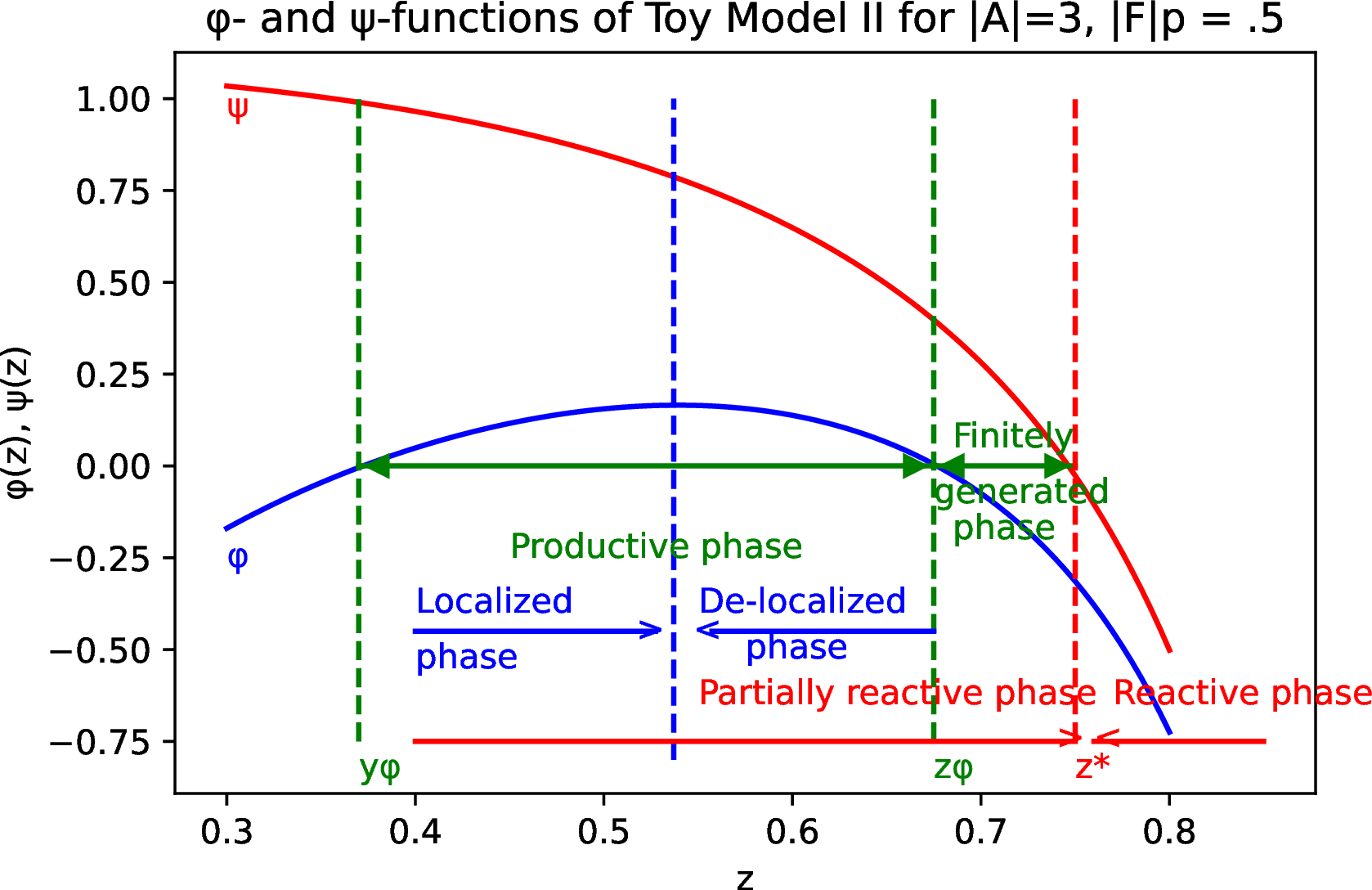
The relatively high value of \(|{\cal F}|p\) chosen in the above Figure is much too large for the above \(p\to 0\) estimates to be even vaguely correct (in particular, \(\phi(z'_{\phi})\simeq 0.165>0\) but \(\log|{\cal A}| - 2 \sqrt{|{\cal F}|p}<0\)). However, this choice has made it possible to plot a large part of the curves \(\phi,\psi\) and observe the transition as \(z\) increases from the de-localized productive phase to the finitely generated phase, and then to the reactive phase. For smaller values of \(p\) (typically, \(|{\cal F}|p\lesssim 10^{-2}\), so that \(\sqrt{|{\cal F}|p}\) is small enough), the numerical agreement with our \(p\to 0\) is good, but it is necessary to zoom out a very small neighborhood of \(z=1\) to observe the transition.

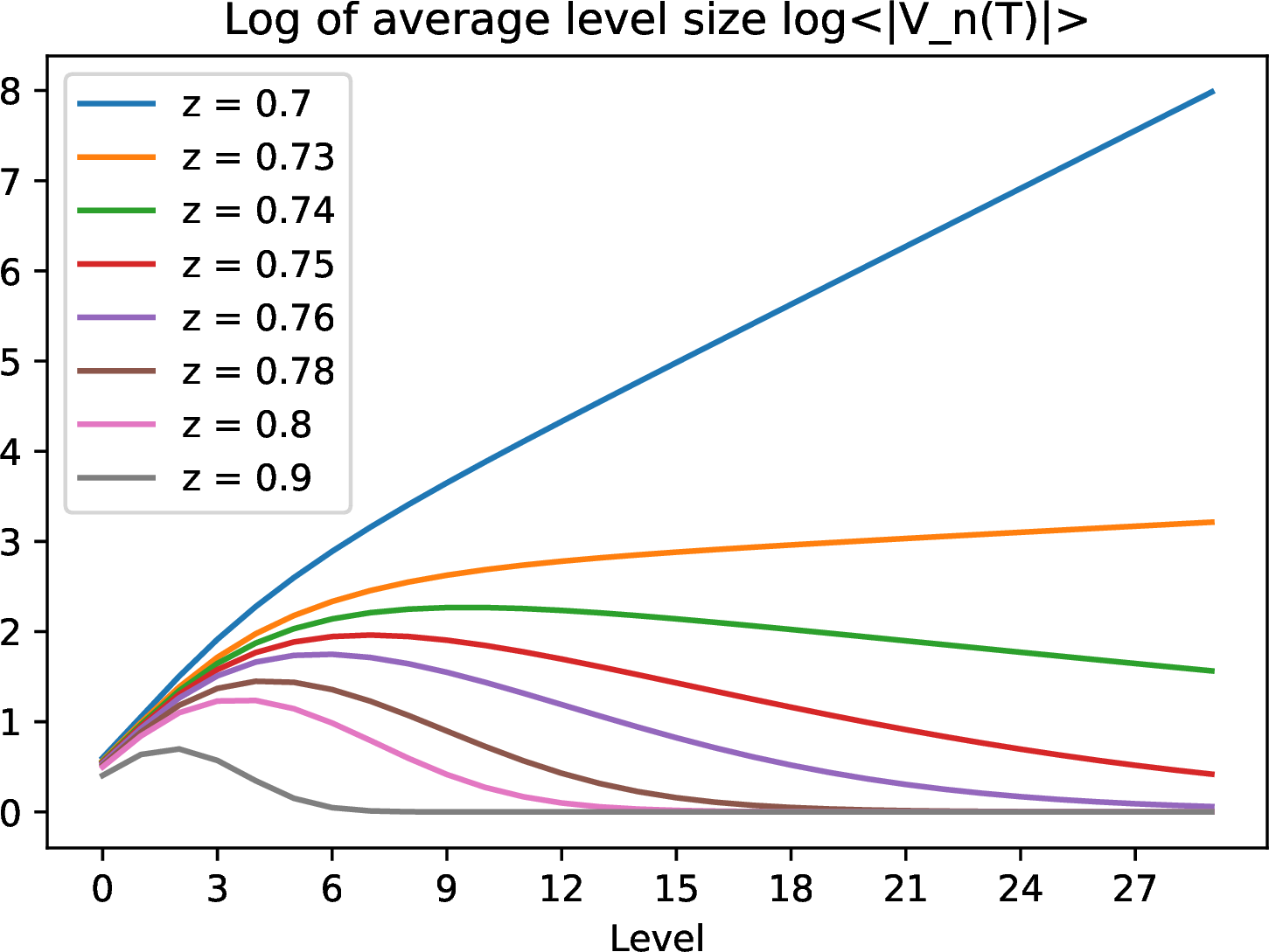
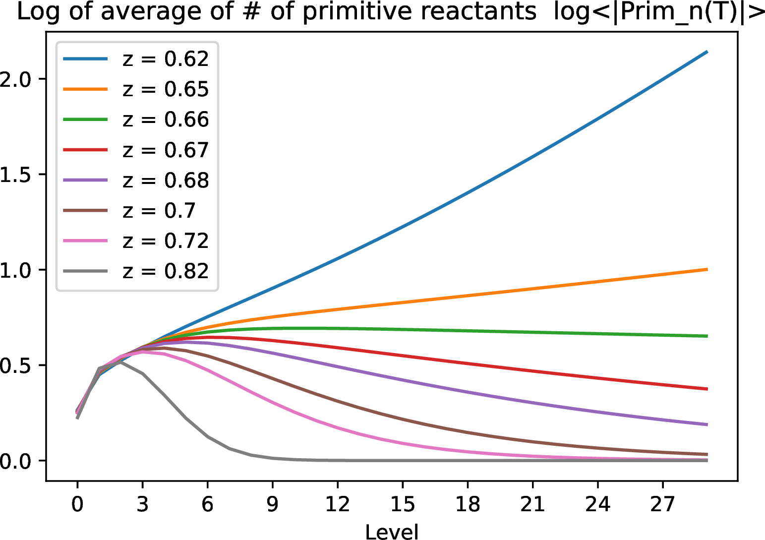
We plot in Figure 14, resp. Figure 15, the prediction of our model for \(\log \langle |V_n({\mathbb{T}})| \rangle\) using (14 ), resp. for \(\log \langle |\mathrm{Prim}_n({\mathbb{T}})| \rangle\) using (16 ). In both cases, we have assumed for definiteness that \(|F|=1\) for all \(F\in {\cal F}\). The phase change at \(z=z^*\), resp. \(z=z_{\phi}\), is quite apparent.
4 Conclusion and perspectives↩︎
We have dealt within the limited scope of this work with a family of "Small-World" chemical reaction models (RRBCN Model I, generalized as RRBCN Model II) dependent on an atom set, a foodset and a fugacity parameter \(z\) conjugate to the complexity index. RRBCN networks were explored along two directions:
•dynamical patterns involving autocatalysis and multistability were systematically investigated and found in the low levels of networks (up to levels 5-6, i.e. 6-7 atoms). Due to CPU time and memory limitations, it seems difficult to extend simulations to much longer molecules.
•statistics of individual mechanisms were established by using an approximate mapping to an inhomogeneous Galton-Watson model. Our predictions agree surprisingly well with numerics. Whereas the model predicts only a finite (though potentially large) number of primitive reactions when reactivity is independent of the complexity index (Model I, \(z=1\)), a number of qualitatively different phases is observed otherwise (Model II). In particular, in an intermediate region for \(z\) far from 0 and 1, there appears a productive phase, characterized by an infinite number of mechanisms with increasing complexity.
The inspiration for the dynamical patterns looked for in §2 comes in part from the above cited article [37], where the authors introduced a toy model of networks of inhibitory interactions based on a sparse graph G playing the same role for dynamics as ConnG (stationary states are indexed by independent subsets of G). Stochastic dynamical simulations displayed very interesting evolutionary features characteristic of glassy dynamics, see also [40] for a study along those lines of the underlying hard-core model on random graphs. It would thus be interesting to see if large, sparse ConnG graphs appear by raising the cut-off level \(n_{max}\), and if conclusions of the above article are also relevant for RRBCN models.
Despite these achievements, our model is a toy model of reactivity, because it fails to deal with the following points:
a larger number of kinetic rankings, depending mainly on the order of magnitude of the kinetic rate, should be distinguished;
molecular graphs in biochemistry are seldom linear. Instead, they branch, form (e.g. aromatic) cycles, and include double and triple bonds, respecting valence rules;
reactions involve electronic rearrangements and protonation/deprotonation steps which allow bond formation/breaking. Thus the product of a reaction is not obtained by pure concatenation/fragmentation of words;
the probability of a bond formation/breaking is strongly dependent on the nature of the atoms involved;
anabolic reactions may involve two reactants, neither of which is in the foodset. Furthermore, some more complicated mechanisms (e.g. 2-2 reactions) may be considered.
However, we have been working on generalizations of our model which go a long way towards overcoming these limitations. The principles are the following:
we need a reasonable prior for kinetic parameters, based on chemical expertise and computational chemistry [41];
looking at functional molecules relevant in extant biology (see e.g. [42]) and prebiotic experiments makes it clear that an overwhelming proportion of molecules is essentially in the form of a linear skeleton, with some short and specific cycles (which can be thought of as additional atoms in our language), and branches of length one (side methyl groups,...), provided functional groups such as carbonyl, carboxyl, etc. are considered as atoms. Thus the 1-derivation model (see Suppl. Info.,
§III.B.2) captures most relevant molecular structures;rearrangements can by-and-large be predicted by the "arrow-pushing diagrams" of undergraduate biochemistry, which change our rules only marginally;
the dependence of kinetic parameters on the atoms makes part of the prior in 1., and can be handled by considering a mapping to a multi-type Galton-Watson model, and using large-deviation theoretic tools to deal with the energy landscape.
Thus only point 5. remains, for which we have no particular strategy. Even before trying to cope with it, much remains to be said about the structure of the reaction network in our toy model. Here only a few preliminary results about the anabolic reaction network, and a remark about the catabolic reaction network, were added in Suppl. Info., showing the relevance of the auxiliary tree model. We already mentioned the difficulty to superpose the two parts of the network (work in progress). But many interesting formulas (not included) can be obtained in various asymptotic regimes. This raises very intriguing questions. There is a small number of chemically interpretable "hyperparameters" in the model, such as \(p,q\); \(z\) (or a level-dependent version of \(z\)); physico-chemical parameters (solvent, pH, temperature...) which change the energy landscape, etc. The first question is: can one infer the value of hyperparameters from experimental data ? Which phase is relevant ? Can one discuss the plausibility of a phase transition as one of the hyperparameters is varied ? Does one observe different statistical behaviors of reaction networks depending on the level, which would point out at a possible chemical evolution towards subnetworks involving longer molecules ?
Funding↩︎
The author did not receive support from any organization for the submitted work.
Conflicts of interest↩︎
The author has no relevant financial or non-financial interests to disclose.
Acknowledgement↩︎
We thank Olivier Rivoire for insightful discussions and helpful comments on the manuscript.
Code availability↩︎
Scripts used to reproduce the analyses and generate the figures reported in this article can be provided upon request to the corresponding author.