Model-Robust and Adaptive-Optimal Transfer Learning for Tackling Concept Shifts in Nonparametric Regression
January 18, 2025
Abstract
When concept shifts and sample scarcity are present in the target domain of interest, nonparametric regression learners often struggle to generalize effectively. The technique of transfer learning remedies these issues by leveraging data or pre-trained models from similar source domains. While existing generalization analyses of kernel-based transfer learning typically rely on correctly specified models, we present a transfer learning procedure that is robust against model misspecification while adaptively attaining optimality. To facilitate our analysis and avoid the risk of saturation found in classical misspecified results, we establish a novel result in the misspecified single-task learning setting, showing that spectral algorithms with fixed bandwidth Gaussian kernels can attain minimax convergence rates given the true function is in a Sobolev space, which may be of independent interest. Building on this, we derive the adaptive convergence rates of the excess risk for specifying Gaussian kernels in a prevalent class of hypothesis transfer learning algorithms. Our results are minimax optimal up to logarithmic factors and elucidate the key determinants of transfer efficiency.
Transfer Learning, Distribution Shift, Nonparametric Regression, Spectral Algorithms, Gaussian Kernels, Misspecification, Minimax Optimality, Adaptivity
1 Introduction↩︎
Nonparametric regression is one of the most extensively studied problems in past decades due to its remarkable flexibility in modeling the relationship between an input \(X\) and output \(Y\). While numerous algorithms have been developed, the strong guarantees of learnability and generalization rely on the fact that there are a sufficient number of training samples and that the future data possess the same distribution as the training. However, training sample scarcity in the target domain of interest and distribution shifts occur frequently in practical applications and deteriorate the effectiveness of most existing algorithms both empirically and theoretically. Transfer learning has emerged as an appealing and promising paradigm for addressing these challenges by leveraging samples or pre-trained models from similar, yet not identical, source domains.
In this work, we study the problem of transfer learning in the presence of the concept shifts for nonparametric regression over some specific reproducing kernel Hilbert spaces (RKHS). Specifically, we posit there are limited labeled samples from the target domain but sufficient labeled samples from a similar source domain where the concept shifted, namely, the conditional distribution of \(Y|X\) changes across domains, which implies the underlying regression function shifts. Hypothesis Transfer Learning (HTL) [1] is the most prevalent framework to tackle concept shift in a two-phase manner by leveraging pre-trained models (hypotheses) from source domains followed by utilizing labeled target samples to learn the shifting, i.e., fine-tune the pre-trained models. HTL algorithms have been extensively studied across various model settings and fine-tuning approaches with theoretical guarantees. Examples include additive linear forms in [2]–[4] and general transformations in [5], [6], among others. Inspired by this framework, a line of research has focused on developing transfer learning algorithms with minimax optimality guarantees. These pursuits facilitate the design and understanding of algorithms from the perspective of fully exploiting source knowledge; see [7]–[12], and more reference therein.
Previous works have primarily focused on transfer learning procedures for model estimation, providing upper bounds or even optimal convergence rates to evaluate the generalization performance given that the model is well-specified, i.e., assuming the specified models in the estimation match the true regression function. In contrast, less attention has been paid to achieving provable and optimal guarantees under misspecified cases despite its prevalence in practical applications. For instance, a considerable body of literature for nonparametric regression assumes the true source and target regression functions reside in certain RKHSs. They derive (nearly) optimal convergence rates of excess risk by assuming the true functions’ regularity is a priori known and the employed RKHSs that contain the estimators are correctly specified in the estimation. [5], [13], [14]. Consequently, such algorithms and analyses are neither robust against misspecification nor adaptive, as the information about the true regression functions is typically unknown in practical applications.
The procedure of HTL typically involves first learning the pre-trained models over the source domain and some intermediate models sequentially and then combining them via some transformations to obtain estimators for the target domains; see Section 2.1. Therefore, it appears promising to exploit some existing well-known robustness results from classical nonparametric methods within the RKHS framework, e.g., [15]–[17], to develop robust transfer procedures with optimality guarantees. These existing robustness results demonstrate that the optimal convergence rate is still attainable even when estimators are learned within misspecified RKHSs. However, such robustness typically depends on the qualification of the learning algorithm (a quantity measuring the algorithm’s fitting capability; see definition in Section 2.2). If the relative regularity of the estimator to the true function deviates significantly from the qualification, these robustness results will no longer hold due to the well-known saturation effect [18], a phenomenon that the convergence rate of the algorithms fails to attain the information-theoretic lower bound. Thus, it is necessary to develop robustness not only against model misspecification but also to overcome the challenges posed by the saturation effect.
Aiming at the gap between theory and practice in the current analysis of HTL, we state the main question of this paper:
How can HTL be truly robust against model misspecification
so that it can achieve provably rate-optimal transfer?
In this work, we answer this question. We first give a new result on the robustness of misspecification for a widely used class of nonparametric methods, termed spectral algorithms, which overcomes saturation effects. We then utilize this result to achieve the main goal. To our knowledge, this work presents the first attempt to address HTL under concept shift that simultaneously fulfills the following two desirable properties: (1) robustness to misspecification of specified RKHSs; and (2) adaptively achieve minimax optimal convergence rates. Our main contributions can be summarized as follows.
Our first result proves that for true regression functions in fractional Sobolev spaces of order \(m\), employing fixed bandwidth Gaussian kernels in arbitrary single-task misspecified spectral algorithms, which will be defined in Section 2.2, attains minimax optimal convergence rates. Additionally, an estimator obtained via standard training and validation achieves the same minimax optimality up to a logarithmic factor. Notably, the optimal order of the regularization parameter \(\lambda\) for achieving non-adaptive rates should decay exponentially, i.e., \(\lambda \asymp \exp\{ -Cn^{\frac{2}{2m+d}} \}\) for a constant \(C\) and sample size \(n\). This robustness result is of independent interest and serves as a complement to classical misspecified kernel methods research.
Methodologically, to answer the main question, we propose a special HTL procedure by imposing spectral algorithms with Gaussian kernels as the learning algorithms in each phase of the HTL. The design of this HTL algorithm leverages the novel robustness against model misspecification exhibited by the Gaussian kernel and is thus free from saturation effects, enabling its capability to consistently and adaptively achieve rate-optimal transfer learning.
Theoretically, we establish the minimax lower bound for the learning problem under concept shifts in terms of excess risk and demonstrate that this special HTL algorithm attains a minimax optimal convergence rate (up to logarithmic factors). The asymptotic optimal rate we obtain reveals that the factor influencing the transfer learning efficiency in HTL is the relative signal strength between true intermediate and source regression functions, where such factors are largely overlooked in existing HTL analyses.
The rest of the paper is organized as follows. In Section 2, we formulate the learning problem, including the concept shifts in nonparametric regression, the HTL framework, and model assumptions. We also briefly introduce the spectral algorithms. In Section 3, we establish both the non-adaptive and adaptive convergence rates for spectral algorithms with fixed bandwidth Gaussian kernels. In Section 4, we present the modified special HTL algorithm for learning the true function with concept shifts, followed by the derivation of minimax optimality analysis and discussions. In Section 5, we conduct simulations to confirm the derived asymptotic convergence rates are optimal. Section 6 provides a detailed review of related works in the context of misspecified kernel methods and transfer learning. Finally, Section 7 concludes the paper and provides discussions.
2 Problem Formulations↩︎
In this section, we set up the problem to be studied in this work. In Subsection 2.1, we formulate the learning problem of nonparametric regression with concept shifts and state the hypothesis transfer learning framework along with the model assumptions. In Subsection 2.2, we introduce the spectral algorithms in classical single-task settings, which serve as the backbone of the learning framework.
2.1 Concept Shifts, Learning Framework and Assumptions↩︎
2.1.0.1 Concept Shifts
Let a compact set \(\mathcal{X}\subset \mathbb{R}^{d}\) be the input space with Lipschitz boundary, and \(\mathcal{Y}\subseteq \mathbb{R}\) be the output space. Suppose there are two unknown probability measures on \(\mathcal{X}\times \mathcal{Y}\), the measure \(P\) for the source domain and \(Q\) for the target domain. One observes \(n_{P}\) i.i.d. labeled source samples \(\mathcal{D}^{P} = \{ (x_{i}^{P},y_{i}^{P}) \}_{i=1}^{n_{P}}\) drawn from distribution \(P\), and \(n_{Q}\) i.i.d. labeled target samples \(\mathcal{D}^{Q} = \{ (x_{i}^{Q},y_{i}^{Q}) \}_{i=1}^{n_{Q}}\) drawn from distribution \(Q\), with \[y_{i}^{P} = f^{P}( x_{i}^{P} ) + \epsilon_{i}^{P} \quad \text{and} \quad y_{i}^{Q} = f^{Q}( x_{i}^{Q} ) + \epsilon_{i}^{Q},\] where \(f^{P}\) and \(f^{Q}\) are the underlying true regression functions, and \(\epsilon_{i}^{P}\) and \(\epsilon_{i}^{Q}\) are i.i.d. random noise with zero mean.
In this work, we consider the concept shifts setting, which is alternatively known as model shifts [19], [20] or posterior drift [9], [21] in different contexts. Specifically, let \(P_{X}\) and \(Q_{X}\) denote the marginal distributions. The concept shift assumes \(P_{X}\) and \(Q_{X}\) are identical while \(P_{Y|X}\) and \(Q_{Y|X}\), i.e., \(f^{P}\) and \(f^{Q}\), are different across the domains. Given the observed samples from both domains, the goal is to construct an estimator \(\hat{f}^{Q}\) that minimizes the excess risk over the target distribution \(Q\), i.e., \(\mathop{\mathrm{E}}_{X\sim Q_{X}}[ ( \hat{f}^{Q}(X) - f^{Q}(X) )^{2} ]\).
2.1.0.2 Learning Framework
In this work, the learning framework we consider is a slight generalization of the hypothesis transfer learning (HTL) procedure adopted from [5], which are both practically and theoretically prevalent for addressing concept shifts.
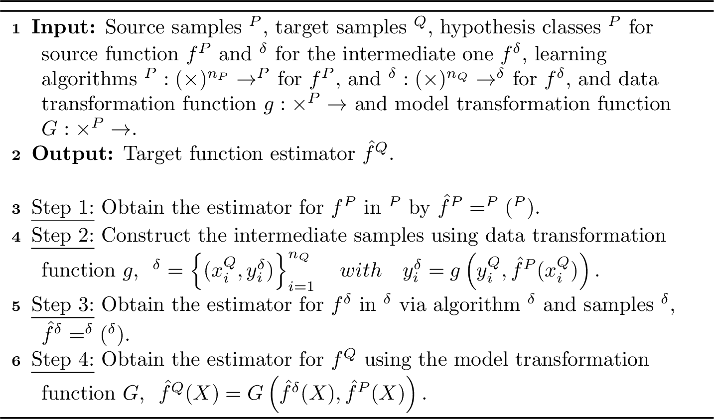
The motivation of Algorithm 1 is to decompose the objective of learning \(f^{Q}\) into learning \(f^{P}\) and \(f^{\delta}\) separately. Here, the source function \(f^{P}\) is less regularized (“more complex”) while the intermediate function \(f^{\delta}\), which represents the shift, is highly regularized (“simple”, e.g., linear functions). Since \(f^{Q}\) is challenging to learn directly with limited target samples, Algorithm 1 facilitates the learning efficiency by learning the “hard” part, \(f^{P}\), effectively using sufficient large source samples and also learning the “simple” part, \(f^{\delta}\), well with limited target samples.
The procedure in Algorithm 1 generalizes many widely used transfer learning algorithms by selecting different \(g\) and \(G\). For example, taking \(g(Y^{Q}, f^{P}(X)) = Y^{Q} - f^{P}(X)\) and \(G(f^{\delta}(X), f^{P}(X)) = f^{P}(X) + f^{\delta}(X)\) represents the offset transfer learning, where the target function is in the additive combination of source and intermediate function. This recovers numerous transfer learning algorithms originated from biased regularization [2], which modify the pre-trained model via additive linear adjustments based on regularized ERM, such as those by [1], [3], [10], [12], to name a few. Additionally, it is shown that in [22], by setting \(g(Y^{Q}, f^{P}(X)) = (Y^{Q} - \tau f^{P}(X))/(1-\tau)\) and \(G(f^{\delta}(X), f^{P}(X)) = (1-\rho)f^{P}(X) + \rho f^{\delta}(X)\) with two varying hyperparameters \(\tau\) and \(\rho\), Algorithm 1 becomes the transfer learning algorithms such as posterior distribution ratio estimation [23] and neural network-based pre-training and fine-tuning [24] given \(\tau\) and \(\rho\) belongs to specific regimes. To establish the theoretical analysis under this learning framework, we impose the following assumption on \(g\) and \(G\), which is standard in most existing HTL literature, such as [1], [5].
Assumption 1. The following conditions hold for data and model transformation function, namely \(g\) and \(G\):
(Invertibility) The model transformation function \(G(x,y)\) is invertible with respect to the first argument, i.e. \(G_{y}^{-1}\) exists, and \(G_{y}^{-1} = g_{y}\).
(Lipschitz continuity) The model transformation function \(G\) is \(L_{1}\)-Lipschitz, i.e., for all \((x,y), (x', y') \in \mathbb{R}^2\), \(|G(x,y) - G(x', y')| \leq L_{1} \sqrt{(x-x')^2 + (y-y')^2}\). Besides, the data transformation function \(g\) is \(L_{2}\)-Lipschitz in second argument, i.e., \(|g(x,y) - g(x, y')| \leq L_{2} |y - y'|\).
(Consistency) For all \(x \in \mathcal{X}\), \[f^{\delta} (x) = \mathop{\mathrm{E}}_{Q}[ g(Y, f^{P}(x)) |X = x ] \quad \text{and} \quad G(f^{\delta}(x), f^{P}(x)) := f^{Q}(x) = \mathop{\mathrm{E}}_{Q}[Y|X = x].\]
The Lipshictz continuity condition guarantees \(\hat{f}^{Q}\) converges to \(f^{Q}\) if both \(\hat{f}^{P}\) and \(\hat{f}^{\delta}\) converge their counterparts. The invertibility condition assures the injection between the values of the target function \(f^{Q}\) and the intermediate function \(f^{\delta}\). Finally, the consistency condition assures that step 3 produces an unbiased estimator for \(f^{\delta}\).
2.1.0.3 Model Assumptions
In this work, we investigate the setting where \(f^{P}\), \(f^{Q}\) and \(f^{\delta}\) reside in some specific RKHSs. Let \(K\) be a symmetric, positive-definite, and continuous kernel function over \(\mathcal{X}\times \mathcal{X}\) that satisfies \(\sup_{x\in \mathcal{X}}K(x,x)\leq \kappa^2\) and denote its associate RKHS as \(\mathcal{H}_{K}(\mathcal{X})\). We consider the stationary kernel, i.e., the value of \(K(x,y)\) only depends on the difference \(x-y\), and write \(K(x-y):= K(x,y)\). For such kernels, one can characterize the RKHS of \(K\) in terms of Fourier transforms when \(\mathcal{X}= \mathbb{R}^{d}\). Let \(\mathcal{F}(f)(\omega)\) denote the Fourier transform of a function \(f\), then by Theorem 10.12 of [25], \[\mathcal{H}_{K}(\mathbb{R}^{d}) = \left\{ f \in L^{2}(\mathbb{R}^{d}) \cap C(\mathbb{R}^{d}) : \frac{\mathcal{F}(f)}{\sqrt{\mathcal{F}(K)}} \in L^{2}(\mathbb{R}^{d}) \right\}.\] When \(\mathcal{X}\) is a subset of \(\mathbb{R}^{d}\), such a definition still captures the regularity of functions in \(\mathcal{H}_{K}(\mathcal{X})\) via a norm equivalency result that holds by the extension theorem [26]. Denote \(\mathcal{W}^{m,p}(\mathcal{X})\) as the Sobolev space with order \(m\). When \(p=2\), the Sobolev space is equivalent to the RKHS of a stationary kernel. The following lemma from [25] describes the norm equivalency.
Lemma 1. Let \(K(x,x')\) be a stationary kernel. Suppose \(\mathcal{X}\) has a Lipschitiz boundary, and the Fourier transform of \(K\) has the following spectral density of \(m\), for \(m > d/2\), \[\label{eqn:32Fourier32Transform32of32reproducing32kernel} c_{1}(1 + \|\cdot\|_{2}^{2})^{m} \leq \mathcal{F}(K)(\cdot) \leq c_{2}(1 + \|\cdot\|_{2}^{2})^{m}.\qquad{(1)}\] for some constant \(0 < c_{1} \leq c_{2}\). Then, the associated RKHS of \(K\), \(\mathcal{H}_{K}(\mathcal{X})\), is norm-equivalent to the Sobolev space \(\mathcal{W}^{m,2}(\mathcal{X}):= H^{m}(\mathcal{X})\).
A prominent class of stationary kernels that satisfy (?? ) is the Matérn kernel [27], which is defined by \[K_{\nu}(x,y ;h) = \frac{2^{1-\nu}}{\Gamma(\nu) }\left( \sqrt{2\nu} \frac{\|x-y\|_2}{h}\right)^\nu K_\nu\left( \sqrt{2\nu} \frac{\|x-y\|_2}{h}\right),\] where \(h\) is the bandwidth and \(K_{\nu}\) is the modified Bessel function of the second kind. The Sobolev space \(H^{m}(\mathcal{X})\) associated with \(K_{\nu}\) satisfied \(m = \nu + d/2\). We let \(H^{m}(\mathcal{X},R)\) represent a ball in the the Sobolev space with radius \(R\), i.e. \(H^{m}(\mathcal{X},R) = \{f : f\in H^{m}(\mathcal{X}), \|f\|_{H^{m}(\mathcal{X})} \leq R \}\). For notational simplification, we abbrivate \(H^{m}(\mathcal{X})\) as \(H^{m}\) and \(H^{m}(\mathcal{X},R)\) as \(H^{m}(R)\) unless otherwise specified. The following assumptions will be made throughout the paper.
Assumption 2 (Smoothness). Suppose that exists positive constants \(m_{P}\), \(m_{Q}\) and \(m_{\delta}\) greater than \(d/2\), and \(R_{P}\), \(R_{Q}\) and \(R_{\delta}\) such that \[f^{P} \in H^{m_{P}}(R_{P}), \quad f^{Q} \in H^{m_{Q}}(R_{Q}) \quad \text{and} \quad f^{\delta} \in H^{m_{\delta}}(R_{\delta}).\]
Assumption 3 (Moment of error). There are constants \(\sigma^{Q}\),\(L^{Q}>0\) such that for any \(r\geq 2\), the noises satisfies \[\mathop{\mathrm{E}}\left[ |\epsilon^{t}|^{r} \mid x \right] \leq \frac{1}{2}r! (\sigma^{t})^{2} (L^{t})^{r-2}, \quad \text{for} \quad t \in \{P,Q\}.\]
Assumption 2 indicates the eigenvalue decay rate (EDR) of the reproducing kernel of these Sobolev spaces is polynomial, which is a standard assumption in nonparametric literature and allows one to obtain the minimax optimal convergence rate directly via classical results [28]. While this assumption does not assert the relationship between \(m_{P}\), \(m_{Q}\) and \(m_{\delta}\), the effectiveness of Algorithm 1 relies on \(m_{\delta}\) being larger, meaning \(f^{\delta}\) is more regularized than \(f^{P}\) and \(f^{Q}\) and thus intuitively aligns with the philosophy of Algorithm 1. For example, when Algorithm 1 takes the offset transfer learning form, it is often assumed \(m_{\delta} \geq m_{P}\) and \(m_{P} = m_{Q}\) [29]. Such “simpler” offset assumptions have also been proven to be effective in other models, e.g., high-dimensional linear works [4], [10], [12] where authors assume the offset coefficients should be sparser than source and target coefficients.
Assumption 3 is also a standard assumption that frequently appears in the kernel method literature [16], [30] to establish theoretical results, which controls the noise tail-probability decay speed.
2.2 Spectral Algorithms↩︎
We now introduce a class of kernel methods for nonparametric regression known as spectral algorithms, which serve as \(\mathcal{A}^{P}\) and \(\mathcal{A}^{\delta}\) in Algorithm 1 in this work. To facilitate simplicity, we introduce the spectral algorithms in a single-task learning setting with the target domain samples \(\mathcal{D}^{Q}\) while an extension to source domain samples is straightforward.
Let \(\mathcal{H}_{K}\) be an RKHS with kernel \(K\). Denote the \(L^{2}\)-space as \(L^{2}(\mathcal{X}, Q_{X})\) (in short \(L^{2}\)). We define the corresponding integral operator \(T_{K}:L^{2} \rightarrow L^{2}\) as \[T_{K}(f)(x^{\prime}) = \int_{\mathcal{X}} K(x,x^{\prime}) f(x) dQ_{X}(x),\] which is a compact operator since it is positive, self-adjoint, and trace-class. Applying Mercer’s theorem yields that there is an at most countable index set \(N\) such that the decomposition \(K(x,x^{\prime}) = \sum_{j\in N}s_{j} e_{j}(x) e_{j}(x^{\prime})\) holds, where \(\{s_{j}\}_{j\in N}\) are the eigenvalues in non-increasing order and \(\{e_{j}\}_{j\in N}\) are the corresponding eigenfunctions, which form an orthonormal basis of \(L^{2}\). For \(x\in \mathcal{X}\), define the evaluation operator as \(K_{x}: \mathcal{H}_{K} \rightarrow \mathbb{R}, f \mapsto \langle f, K_{x} \rangle_{\mathcal{H}_{K}}\) and its adjoint operator \(K_{x}^{*}: \mathbb{R}\rightarrow \mathcal{H}_{K}, y \mapsto yK_{x}\). We define the target sample covariance operator \(T_{K,n}^{Q}:\mathcal{H}_{K}\rightarrow \mathcal{H}_{K}\) and the target sample bias function \(g_{n}^{Q}:\mathbb{R}^{n} \rightarrow \mathcal{H}_{K}\) as \[T_{K,n}^{Q} := \frac{1}{n_{P}}\sum_{i=1}^{n_{Q}}K_{x_{i}^{Q}}^{*}K_{x_{i}^{Q}}\quad \text{and} \quad g_{n}^{Q}:=\frac{1}{n_{Q}} \sum_{i=1}^{n} K_{x_{i}^{Q}}^{*}y_{i}^{Q}.\]
In the classical single-task non-parametric regression problem, the goal is to obtain \(\hat{f}^{Q}\) from \(\mathcal{H}_{K}\) based on the target samples \(\mathcal{D}^{Q}\) to achieve small risk in \(L^{2}\). Thus, it is natural to obtain \(\hat{f}^{Q}\) by minimizing the empirical squared loss over \(\mathcal{H}_{K}\), i.e. \[\label{eqn:32empirical32loss32minimization32problem} \hat{f}^{Q} = \underset{f\in \mathcal{H}_{K}}{\operatorname{argmin}} \frac{1}{n} \sum_{i=1}^{n_{Q}} \left( f(x_{i}^{Q}) - y_{i}^{Q} \right)^2,\tag{1}\] which gives \(\hat{f}^{Q}\) as the solution of the empirical, linear equation, \(T_{K,n}^{Q}f = g_{n}^{Q}\). However, solving this equation is an ill-posed inverse problem as the inverse of the sample covariance operator, \(T_{K,n}^{Q}\), in general, does not exist. In inverse problems and statistical learning, a common approach to address this issue is to replace the inverse of \(T_{K,n}^{Q}\) with a regularized operator. This replacement corresponds to selecting a specific filter function, which leads to the formulation of spectral algorithms [18], [31], [32].
Definition 1 (Filter function). The class of functions \(\{ \phi_{\lambda} : [0,\kappa^2] \rightarrow \mathbb{R}^{+} | \lambda \in \mathbb{R}\}\) are said to be filter functions with qualification \(\tau \geq 0\) and regularization parameter \(\lambda\), if there exists some positive constants \(E, F_{\tau} < \infty\) such that the following two conditions hold: \[\label{eqn:32filter32function32condition321} \sup _{\beta \in[0,1]} \sup _{\lambda \in \Lambda} \sup _{\left.u \in[ 0, \kappa^2\right]}\left|u^\beta \phi_{\lambda}(u)\right| \lambda^{1-\beta} \leq E ,\qquad{(2)}\] \[\label{eqn:32filter32function32condition322} \sup _{\beta \in[0, \tau]} \sup _{\lambda \in \Lambda} \sup _{\left.u \in[ 0, \kappa^2\right]}\left|\left(1-\phi_{\lambda}(u) u\right)\right| u^\beta \lambda^{-\beta} \leq F_\tau.\qquad{(3)}\]
The motivation for introducing the class of filter functions is that \(\phi_{\lambda}\) is analogous to the function \(\phi(t) = t^{-1}\) but with better behavior around \(0\), e.g. \(\phi_{\lambda}\) is bounded by \(\lambda^{-1}\). We now define the corresponding spectral algorithms given a specific filter function \(\phi_{\lambda}\).
Definition 2 (Spectral algorithm). Let \(\phi_{\lambda}\) be a filter function with parameter \(\lambda\). Given the target samples \(\mathcal{D}^{Q}\), the estimator from the spectral algorithm is given by \[\hat{f}^{Q} = \phi_{\lambda}(T_{K,n}^{Q}) g_{n}^{Q}.\]
Here, the filter function \(\phi_{\lambda}\) acts on the eigenvalues of the self-adjoint finite-rank sample covariance operator \(T_{K,n}\). Different filter functions lead to different types of regularization. We list some of the commonly used spectral algorithms in the following examples. For more examples of spectral algorithms, we refer readers to [33].
Kernel Ridge Regression (KRR): The choice of Tikhonov filter function \(\phi_{\lambda}(z) = (z + \lambda)^{-1}\) corresponds to kernel ridge regression. In this case, \(\tau= E = F_{\tau}=1\).
Gradient Descent (GD) and Gradient Flow (GF): The choice of \(\phi_{\lambda}(z) = \eta \sum_{k=1}^{t-1} (1 - \eta z)^{k}\) where \(\lambda = (\eta t)^{-1}\)
corresponds to gradient descent where \(\eta > 0\) is a constant step size. Gradient descent with more complex update rules can be expressed in terms of filter functions as well [34], [35]. For infinitely small step size, the choice of \(\phi_{\lambda}(z) = (1 - \exp\{-\frac{z}{\lambda}\}) / z\) corresponds to gradient flow. In both cases, \(\tau\) could be any positive number, \(E=1\), and \(F_{\tau}=(\tau/e)^{\tau}\).
Kernel Principal Component Regression (KPCR): The choice of spectral cut-off function \(\phi_{\lambda}(z) = z^{-1} \mathbb{1}_{z\geq \lambda}\) corresponds to Kernel Principal Component Regression, which is motivated by using finite components to recover \(T_{K,n}^{Q}\). In such case, \(\tau\) could be any positive number, \(\tau= E = F_{\tau}=1\).
3 Spectral Algorithms with Gaussian Kernels↩︎
Observing that Algorithm 1 obtains the \(\hat{f}^{P}\) and \(\hat{f}^{\delta}\) through two sequential and independent spectral algorithms, \(\mathcal{A}^{P}\) and \(\mathcal{A}^{\delta}\), we first consider the robustness and adaptivity for spectral algorithms under the classical learning setting (i.e., recovering \(f^{Q}\) with \(\mathcal{D}^{Q}\) solely), and then apply the results to Algorithm 1 to answer the main question of this work. Specifically, this section begins with a warm-up example to demonstrate why existing misspecified results are insufficient and highlights the motivation for using Gaussian kernels. We then present the non-adaptive and adaptive minimax optimal convergence rate for spectral algorithms with Gaussian kernels, followed by detailed discussions.
3.1 Warm-up: Misspecification with Optimal Rate and Saturation Effect↩︎
We first review some existing robustness results on misspecified spectral algorithms and the saturation effect.
Proposition 1 (Target-only Learning). For a symmetric and positive semi-definite kernel \(K:\mathcal{X}\times \mathcal{X}\rightarrow \mathbb{R}\), let \(\mathcal{H}_{K}\) be the RKHS associated with \(K\) [25]. Let \(\hat{f}^{Q} \in \mathcal{H}_{K}\) be the spectral algorithms estimator in Definition 2 with qualification \(\tau\) and regularization parameter \(\lambda\), imposed kernel as \(K\) and target sample \(\mathcal{D}^{Q}\). The convergence rate of excess risk of \(\hat{f}^{Q}\) is given as follows.
(Misspecification) Suppose the imposed kernel \(K\) satisfies condition ?? with order \(m_{Q}' > \frac{d}{2}\), that is, its associated RKHS, \(\mathcal{H}_{K}\), is norm-equivalent to \(H^{m_{Q}'}\). Furthermore, given \(\lambda \asymp n^{- \frac{2m_{Q}'}{2m_{Q} + d} }\) and \(\gamma = \min\{2\tau, \frac{m_{Q}}{m_{Q}'} \}\), then \[\left\| \hat{f}^{Q} - f^{Q} \right\|_{L^{2}}^{2} = O_{\mathbb{P}} \left( n_{Q}^{-\frac{2\gamma m_{Q}'}{2\gamma m_{Q}' + d}} \right).\]
(Saturation Effect) For \(m_{Q}' < \frac{m_{Q}}{2\tau}\) and any choice of parameter \(\lambda(n_{Q})\) satisfying that \(\lambda(n_{Q})\rightarrow 0\), we have \[\left\| \hat{f}^{Q} - f^{Q} \right\|_{L^{2}}^{2} = \Omega_{\mathbb{P}} \left( n_{Q}^{-\frac{4 \tau m_{Q}'}{4\tau m_{Q}' + d}} \right).\]
When \(m_{Q}' = m_{Q}\), the misspecified result becomes well-specified and can be found in a line of past work [36], [37]. The misspecified result comes from a combination (with a modification) of Theorem 15 and 16 in [17] and Theorem 1 in [30]. The saturation effect is proved by Corollary 3.2 in [38]. Given the fact that the minimax optimal rate is \(n^{-2m_{Q}/(2m_{Q}+d)}\) when \(f^{Q}\in H^{m_{Q}}\), Proposition 1 indicates that even when the imposed RKHS \(\mathcal{H}_{K}\) is misspecified (and thus the estimator \(\hat{f}^{Q}\)), the minimax optimal rate is still attainable when \(m_{Q}' \geq m_{Q}/2\tau\) with appropriately chosen \(\lambda\). However, if \(m_{Q}' < m_{Q}/2\tau\), i.e., the true function is much smoother than the estimator itself, the saturation effect occurs, i.e., there is a persistent gap between the lower bound of the estimator and the information-theoretic lower bound of the learning problem.
The misspecified result in Proposition 1 suggests a potential solution to the main question of this work: imposing appropriately misspecified kernels, such as Matérn kernels, in \(\mathcal{A}^{P}\) and \(\mathcal{A}^{\delta}\) to attain robustness against model misspecification while achieving optimal rate. Nonetheless, such a solution still faces two problems: (1) Non-adaptivity, i.e., one still needs to know the true smoothness when tuning \(\lambda\); (2) Saturation risk, i.e., using spectral algorithms with finite qualifications \(\tau\) but a less smooth kernel is imposed. Although the former can be potentially addressed by some data-driven adaptive approaches, the second one is more problematic, as choosing a less smooth kernel may permanently prevent achieving the optimal rate. While saturation effects can be mitigated by selecting specific spectral algorithms with arbitrarily large qualifications, this restricts the flexibility in choosing \(\mathcal{A}^{P}\) and \(\mathcal{A}^{\delta}\), eliminating the potential benefits that can be gained from customizing these general algorithms under different application scenarios.
Therefore, there is a clear need for a misspecified kernel that can be robust against both model misspecification and the potential saturation effect across arbitrary spectral algorithms. Formally, for \(f^{Q} \in H^{m_{Q}}\) with any \(m_{Q} > d/2\), imposing such a kernel in the spectral algorithms would ensure that, regardless of the spectral algorithm’s qualification, there always exists an optimal \(\lambda\) such that the minimax optimal convergence rate is achievable.
3.2 Opimal Convergence Rate with Gaussian Kernels↩︎
We start with the motivation for considering the Gaussian kernels. As shown in Proposition 1, when the imposed RKHS’s smoothness \(m_{Q}'\) is greater than the quantity \(m_{Q}/2\tau\), there always exists an optimal \(\lambda\) such that the minimax optimal rate is attainable. This indicates that the most prominent issue that causes the saturation effect is the large relative smoothness of \(f^{Q}\) to \(\hat{f}^{Q}\), i.e., estimating a smooth function with a much less smooth estimator. Thus, a feasible strategy is always to employ a Matérn kernel with large smoothness so that the estimator \(\hat{f}^{Q}\) is obtained from a smoother Sobolev space than the one where \(f^{Q}\) resides. However, precisely determining the appropriate smoothness to impose on \(\hat{f}^{Q}\) is challenging since the true smoothness \(m_{Q}\) is typically unknown. To this end, we consider using the fixed bandwidth Gaussian kernel, which is further motivated by the following fact.
- The RKHS associated with the isotropic Matérn kernel \(K_{\nu}\) [27] is isomorphic to the Sobolev space \(H^{\nu + \frac{d}{2}}\). Moreover, the Gaussian kernel is the limited of the Matérn kernel, i.e. \[\lim_{\nu \rightarrow\infty} K_{\nu}(x; h) = \exp \left( - \frac{\|x-y\|_{2}^{2}}{2h^2} \right), \quad x,y \in \mathbb{R}^{d},\] and the RKHS associated with the Gaussian kernel is contained in the Sobolev space \(H^{m_{Q}}\) for any \(m_{Q} > d/2\) [39].
Thus, in using the Gaussian kernel, one might expect to achieve the minimax optimal rate with a feasible \(\lambda\) and overcome the saturation effect since its corresponding RKHS consists of functions that are consistently “smoother” than \(f^{Q}\).
Our first result proves that there exists an optimal order of \(\lambda\) such that the spectral algorithms with Gaussian kernels attain the optimal convergence rate.
Theorem 1 (Non-Adaptive Rate). Under Assumptions 2 and 3, let the imposed kernel, \(K\), be the fixed bandwidth Gaussian kernel and the estimator be \(\hat{f}^{Q} = \mathcal{A}_{K,\lambda}(\mathcal{D}^{Q})\), where \(\mathcal{A}_{K,\lambda}\) is an arbitrary spectral algorithm with kernel \(K\) and regularization parameter \(\lambda\). By choosing \(log(1/\lambda) \asymp n^{\frac{2}{2m_{Q}+d}}\), for any \(\delta \in (0,1)\) and sufficiently large \(n_{Q}\geq 1\), with probability at least \(1-\delta\), we have \[\left\| \hat{f}^{Q} - f^{Q} \right\|_{L^{2}}^{2} \leq C \left(\log \frac{4}{\delta} \right)^2 n_{Q}^{-\frac{2m_{Q}}{2m_{Q} + d}},\] where \(C\) is a constant independent of \(n_{Q}\) and \(\delta\).
Remark 1. Establishing the upper bound requires a technical assumption (Assumption 4 in Appendix 8), which uniformly bounds \(\sum_{j=1}^{\infty} \frac{s_{j}}{s_{j}+\lambda} e_{j}^{2}(x)\) by the effective dimension. It is slightly weaker than the commonly assumed uniformly boundedness of the eigenfunction of \(T_{K}\), a rather standard assumption in nonparametric literature, particularly under misspecified case; see [40]. Notably, whether this assumption holds for Gaussian kernels is, to the best of our knowledge, not addressed in existing literature, necessitating making such assumptions when considering specific kernels, like Matérn kernels, in misspecified kernel research; see [17].
Despite the minimax optimality of the spectral algorithm demonstrated in Theorem 1, a key practical challenge is that choosing optimal \(\lambda\) still requires knowing \(m_{Q}\). To address this, we developed an adaptive rate when the smoothness parameter \(m_{Q}\) is unknown a priori. The adaptive procedure is based on a standard training and validation approach [41]. Specifically, we construct a finite set that is a finite arithmetic sequence, i.e., \(\mathcal{M}= \{m_{\min}< \cdots < m_{\max}\}\) where \(\{m_{i}\}\) satisfy \(m_{\min}>d/2\), \(m_{\max}\) large enough such that \(m_{Q}\leq m_{\max}\) and \(m_{i} - m_{i-1}\asymp 1/\log n_{Q}\). We then split dataset \(\mathcal{D}^{Q}\) into \(\mathcal{D}_{1}^{Q} := \{(x_{1}^{Q},y_{1}^{Q}),\cdots,(x_{j}^{Q},y_{j}^{Q})\}\) and \(\mathcal{D}_{2}^{Q} = \mathcal{D}^{Q} \backslash \mathcal{D}_{1}^{Q}\). The adaptive estimator is obtained by following the training and validation approach.
(Training): For each \(m \in \mathcal{M}\), compute the non-adaptive estimator \(\hat{f}_{\lambda_{m}}^{Q} = \mathcal{A}_{K,\lambda_{m}}(\mathcal{D}_{1}^{Q})\) with the spectral algorithm \(\mathcal{A}_{K,\lambda_{m}}\) and dataset \(\mathcal{D}_{1}^{Q}\). The regularization parameter \(\lambda_{m}\) is chosen as \(\lambda = \exp\{ -Cn^{2/2m + d} \}\) for some constant \(C\) based on Theorem 1.
(Validation): Selecting the \(\hat{f}_{\lambda_{m}}^{Q}\) that minimizes empirical \(L^{2}\) error over \(\mathcal{D}_{2}^{Q}\) as the adaptive estimator \(\hat{f}_{\hat{\lambda}}^{Q}\).
The following theorem shows the adaptive estimator from the aforementioned training and validation approach attains optimal rate up to a logarithmic factor in \(n_{Q}\).
Theorem 2 (Adaptive Rate). Under the same conditions of Theorem 1. Then, for \(\delta \in (0,1)\), with probability \(1-\delta\), we have \[\label{eqn:32target-only32adaptive32rate} \left\| \hat{f}_{\hat{\lambda}}^{Q} - f^{Q} \right\|_{L^{2}}^{2} \leq C \left( \log\frac{4}{\delta} \right)^2 \left(\frac{n_{Q}}{\log n_{Q}} \right)^{-\frac{2m_{Q}}{2m_{Q} +d}},\qquad{(4)}\] where \(C\) is a constant independent of \(n_{Q}\) and \(\delta\).
Remark 2. We note that the aforementioned training and validation approach is not the only way to achieve the adaptive procedure. To obtain the adaptive rate, one can also employ other widely used data-driven methods or model selection procedures, such as Lepski’s method [42].
3.3 Discussion↩︎
Theorem 1 shows that the excess risk of spectral algorithms with fixed bandwidth Gaussian kernels can attain the minimax optimal convergence rate without restriction on the qualification. From another perspective, it offers a robust solution to avoid the potential saturation effect in spectral algorithms with low qualifications.
It is interesting to note that even though the motivation for imposing Gaussian kernels is that the Gaussian kernel is the limit of Matérn kernel \(K_{m_{Q}'}\) as \(m_{Q}'\rightarrow\infty\), the misspecified case in Proposition 1 can never substitute our result. Specifically, setting the smoothness parameter \(m_{Q}'\) as infinity in Proposition 1, the polynomial decay form of \(\lambda\) never makes the optimal order of \(\lambda\) trackable since \(\lim_{m_{Q}' \rightarrow \infty} n_{Q}^{-2m_{Q}'/(2m_{Q}+d) } = 0\), and only indicates that the optimal \(\lambda\) should converge to \(0\) much faster than the polynomial form. In contrast, our result explicitly reveals that the optimal order of \(\lambda\) should decay exponentially.
This exponential decay form of the optimal \(\lambda\) originates from controlling the approximation error. The misspecified results in Proposition 1 rely on the standard real interpolation technique to control the approximation error. It allows one to expand the intermediate term \(f_{\lambda}^{Q}\) (see definition in Appendix 8) and the true function \(f^{Q}\) under the same basis, making the approximation error scale as \(\lambda^{m_{Q}/m_{Q}'}\|f^{Q}\|_{H^{m_{Q}}}\) and the optimal \(\lambda\) decays polynomially like Proposition 1. This technique is widely used in many misspecified kernel literature. However, in our case, the intermediate term lies in the RKHS of Gaussian kernels, making expanding \(f_{\lambda}^{Q}\) and \(f^{Q}\) under the same basis no longer feasible. The technique we used to prove the Theorem 1 is the Fourier transform of the Gaussian kernel, which allows us to bound the approximation error by \(log(1/\lambda)^{-m_{Q}} \| f^{Q} \|_{H^{m_{Q}}}^{2}\) and consequently reveals this exponential decay order of \(\lambda\). We refer readers to Appendix 8 for more details.
| Paper | Imposed RKHS | Rate | \(\lambda\) | \(h\) | Type |
|---|---|---|---|---|---|
| [17] | \(H^{m_{Q}'}, m_{Q}'>\frac{m_{Q}}{2}\) | \(n_{Q}^{-\frac{2m_{Q}}{2m_{Q} + d}}\) | \(n_{Q}^{-\frac{2m_{Q}'}{2m_{Q} + d}}\) | \(-\) | KRR |
| [30] | \(H^{m_{Q}'}, m_{Q}'>\frac{m_{Q}}{2\tau}\) | \(n_{Q}^{-\frac{2m_{Q}}{2m_{Q} + d}}\) | \(n_{Q}^{-\frac{2m_{Q}'}{2m_{Q} + d}}\) | \(-\) | |
| [43] | \(\mcH_{K}\) | \(n_{Q}^{-\frac{2m_{Q}}{2m_{Q} + d}+ \xi}, \forall \xi> 0\) | \(n_{Q}^{-1}\) | \(n_{Q}^{-\frac{1}{2m_{Q} + d} }\) | |
| [44] | \(\mcH_{K}\) | \(n_{Q}^{-\frac{2m_{Q}}{2m_{Q} + d}}\log^{d+1}(n)\) | \(n_{Q}^{-1}\) | \(n_{Q}^{-\frac{1}{2m_{Q} + d} }\) | |
| Theorem [thm:32non-adaptive32rate32of32SA32with32Gaussian] in this work | \(\mcH_{K}\) | \(n_{Q}^{-\frac{2m_{Q}}{2m_{Q} + d}}\) | \(\exp\{-Cn_{Q}^{\frac{2}{2m_{Q} + d}}\}\) | \(-\) |
Lastly, to further highlight our findings, we summarize some state-of-the-art results (with slight modifications to align with our setting) that consider general, Matérn, or Gaussian misspecified kernels for the spectral algorithms (or their special cases) and highlight our result in Table 1. We refer readers to Section 6 for a detailed literature review.
The pattern of the \(\lambda\) in this work differs significantly from previous attempts that justify the minimax optimality of the misspecified fixed bandwidth Matérn kernel or variable bandwidth Gaussian kernel in statements. Especially in the regime of variable bandwidth, given both \(\gamma\) and \(\lambda\) decay polynomially in \(n_{Q}\), [43] showed that the convergence rate could be arbitrarily close to the optimal rate, while [44] attained the optimal rate (up to a logarithmic factor) under the so-called DIM condition. However, we would like to note that these variable Gaussian results are not directly comparable to ours due to the difference in model settings and assumptions. For example, these two works consider regularized ERM problems, allowing for loss functions beyond the square ones. They also assumed data distributions are bounded, whereas we considered a moment-based error assumption.
4 Robust and Adaptive Hypothesis Transfer Learning↩︎
In this section, we first present a special version of Algorithm 1 based on the results in Section 3. Then, we theoretically analyze the minimax optimality of this special HTL algorithm in Subsection 4.2 and discuss its insights in Subsection 4.3.
4.1 Methodology↩︎
A key observation of Algorithm 1 is that the estimators \(\hat{f}^{P}\) and \(\hat{f}^{\delta}\) are learned separately on two datasets \(\mathcal{D}^{P}\) and \(\mathcal{D}^{\delta}\) using the spectral algorithms \(\mathcal{A}^{P}\) and \(\mathcal{A}^{\delta}\), respectively. Consequently, achieving robust and adaptive HTL with rate-optimal guarantees reduces to achieving the same goal in learning \(f^{P}\) and \(f^{\delta}\) individually. Recall that in a single dataset learning case, Theorem 2 shows that the desired results can be obtained by imposing Gaussian kernels. Building on this observation, we introduce Robust and Adaptive Hypothesis Transfer Learning (RAHTL) estimator, defined via Algorithm 1 as follows: \[\hat{f}^{Q} = G\left ( \hat{f}_{\hat{\lambda}_{\delta}}^{\delta}, \hat{f}_{\hat{\lambda}_{P}}^{P} \right).\] Here, \(\hat{f}_{\hat{\lambda}_{P}}^{P} = \mathcal{A}_{K,\hat{\lambda}_{P}}^{P}(\mathcal{D}^{P})\) and \(\hat{f}_{\hat{\lambda}_{\delta}}^{\delta} = \mathcal{A}_{K,\hat{\lambda}_{\delta}}^{\delta}(\mathcal{D}^{\delta})\) are adaptive estimators obtained using selected spectral algorithms with Gaussian kernels of fixed bandwidth \(K\). \(\mathcal{D}^{P}\) is the source dataset and \(\mathcal{D}^{\delta}\) is the intermediate dataset generated by applying data transformation function \(g\) to \(\mathcal{D}^{p}\) and the pre-trained estimator \(\hat{f}_{\hat{\lambda}_{P}}^{P}\).
4.2 Optimal Convergence Rate Analysis↩︎
Based on Assumption 2, the parameter space for the learning problem is defined as follows, \[\Theta(R_{P},R_{\delta},m_{P},m_{\delta}) = \left\{ (P, Q): \left\|f^{P}\right\|_{H^{m_{P}}}\leq R_{P}, \left\|f^{\delta}\right\|_{H^{m_{\delta}}} \leq R_{\delta} \right\}.\] Here, \(R_{\delta}\) mathematically quantifies the similarity between the source and target functions as a small \(R_{\delta}\) indicates the \(f^{P}\) and \(f^{Q}\) are more similar. We note that such an upper bound for the distance between parameters or models from both domains is often necessary to establish rigorous optimality in many concept shift settings. Examples include \(\ell^{1}\) or \(\ell^{0}\) distance in high-dimensional setting [10], [12], Fisher-Rao distance in low-dimensional setting [45], RKHS distance in functional setting [14], etc.
Our first result specifies the minimax lower bound, which elucidates the information-theoretic difficulty of the transfer learning problem.
Theorem 3 (Lower Bound). For \(\delta \in (0,1)\), with probability \(1-\delta\), we have the following lower bound hold: \[\inf_{\tilde{f}} \sup_{\Theta(R_{P},R_{\delta},m_{P},m_{\delta})} \mathbb{P} \left\{ \left\| \tilde{f} - f^{Q} \right\|_{L^{2}}^2 \geq C_{1} \delta R^{2} \left( n_{P}^{-\frac{2m_{P}}{2m_{P}+d}} + C_{2}\xi n_{Q}^{-\frac{2m_{\delta}}{2m_{\delta}+d}} \right) \right\} \geq 1 - \delta,\] where \(\xi\propto R_{\delta}^{2}/R_{P}^{2}\) and \(C_{1}\), \(C_{2}\) are constants independent of \(n_{P}\), \(n_{Q}\), \(R_{P}\), \(R_{\delta}\), and \(\delta\). The \(\inf\) is taken over all possible estimators \(\tilde{f}\) based on sample \(\mathcal{D}^{P}\) and \(\mathcal{D}^{P}\).
The next theorem provides the upper bound of the excess risk for the RAHTL estimator and shows that it is minimax optimal up to logarithmic factors.
Theorem 4 (Upper Bound). Suppose the Assumption 2, and 3 hold, and \(n_{P}\) and \(n_{Q}\) are sufficiently large but still in transfer learning regime (\(n_{P} \gg n_{Q}\)). Denote the \(\hat{f}^{Q}\) as the RAHTL estimator. For \(\delta \in (0,1)\), with probability \(1-\delta\), we have \[\label{eqn:32RAHTL32upper32bound} \begin{align} \left\| \hat{f}^{Q} - f^{Q} \right\|_{L^{2}}^{2} \leq C_{1} & \left(\log \frac{12}{\delta}\right)^2 \left( 1 + \frac{\sigma_{P}^{2}}{R_{P}^2} \vee \frac{\sigma_{Q}^{2}}{R_{\delta}^2} \right) R^2 \\ & \;\left\{ \left(\frac{n_{P}}{\log n_{P}}\right)^{-\frac{2m_{P}}{2m_{P}+d}} + C_{2}\xi \left(\frac{n_{Q}}{\log n_{Q}}\right)^{-\frac{2m_{\delta}}{2m_{\delta}+d}} \right\}, \end{align}\qquad{(5)}\] where \(\xi \propto R_{\delta}^{2}/R_{P}^{2}\) and \(C_{1}\), \(C_{2}\) are constants independent of \(n_{P}\), \(n_{Q}\), \(R_{P}\), \(R_{\delta}\), and \(\delta\).
Theorem 4 indicates that the convergence rate of the estimator \(\hat{f}^{Q}\) consists of two components: the first term is pre-training error which represents the error of learning \(f^{P}\) with the source samples, while the second term is the fine-tuning error, which arises from learning the intermediate function \(f^{\delta}\) with the constructed samples.
Remark 3. Since the excess risk of \(\hat{f^{Q}}\) can be bounded by \(\|\hat{f}^{P} - f^{P}\|_{L^{2}}^2 + \|\hat{f}^{\delta} - f^{\delta}\|_{L^{2}}^2\) using the Lipschitz continuity of the model transformation function \(G\), it appears that the upper bound can be obtained by applying Theorem 2 on \(\|\hat{f}^{P} - f^{P}\|_{L^{2}}^2\) and \(\|\hat{f}^{\delta} - f^{\delta}\|_{L^{2}}^2\) individually. However, there is actually an additional error, stemming from \(\|\hat{f}^{\delta} - f^{\delta}\|_{L^{2}}^2\), induced by using the estimator \(\hat{f}^{P}\) instead of using true source function \(f^{P}\) to construct the intermediate labels \(\{y_{i}^{\delta}\}_{i=1}^{n_{Q}}\). When \(\mathcal{A}^{P}\) and \(\mathcal{A}^{\delta}\) are both specified as KRR to in Algorithm 1, [5] showed that this error is an amplified version of the pre-training error, which is proportional to the product of the pre-training error and a monotonic increase function of \(n_{Q}\), i.e., \(n_{Q}^{\frac{2}{2m_{P}+d}}\log(n_{Q}) \cdot \|\hat{f}^{P} - f^{P}\|_{L^{2}}^2\). A similar conclusion is made in [13]. Their analysis is based on using the algorithmic stability technique for KRR and is claimed to be nearly tight. However, for sufficiently large but fixed \(n_{P}\) and growing \(n_{Q}\), such bounds suggest that the excess risk of \(\hat{f}^{Q}\) will explode. This is counterintuitive since when there is a sufficiently good pre-trained estimator \(\hat{f}^{P}\), the estimated intermediate label will also be close to the true intermediate label, leading to sufficiently good \(\hat{f}^{\delta}\).
In contrast, we refine the error analysis and show that the error induced by using \(\hat{f}^{P}\) in constructing \(y_{i}^{\delta}\) is bounded by the pre-training error \(\|\hat{f}^{P} - f^{P}\|_{L^{2}}^2\); see Theorem 7 for details. This thus makes the excess risk of \(\hat{f}^{Q}\) receive no amplification and is minimax optimal. Notably, [29] obtained a similar result in the KRR case by using the property of Tikhonov filter function. However, directly extending those arguments to our current setting is not feasible, which necessitates a different treatment. To address this, we bound this error using the operator techniques adapted from [46]. For further details, please refer to Appendix 9.
4.3 Discussion↩︎
We now discuss the minimax optimal rate in Subsection 4.2 to provide insights to better understand the transfer efficiency. Specifically, we explore how the source samples improve the learning efficiency over the target domain and identify what factors contribute to higher efficiency. These insights are derived by comparing the convergence rates between target-only learning ?? and transfer learning ?? . However, without explicitly assuming the relationship between \(m_{Q}\), \(m_{P}\), and \(m_{\delta}\) in Assumption 2, it is hard to compare these rates directly. In the following proposition, we show that the target smoothness \(m_{Q}\) can be linked to \(m_{P}\) and \(m_{\delta}\) given the model transformation function \(G\) belongs to certain smooth function classes.
Proposition 2. Suppose Assumption 2 holds, and denote \[m_{1} = \begin{cases} m_{P} & \text{if m_{P} is an integer}\\ \lfloor m_{P} \rfloor + 1 & \text{otherwise}, \end{cases} \quad \text{and} \quad m_{2} = \begin{cases} m_{\delta} & \text{if m_{\delta} is an integer}\\ \lfloor m_{\delta} \rfloor + 1 & \text{otherwise}. \end{cases}\] Further, suppose the model transformation function \(G\) belongs to the smooth function class \(C^{\max(m_{1},m_{2})}\). Then, for all \(X\in \mathcal{X}\), the Sobolev smoothness of \(f^{Q}(X) := G(f^{\delta}(X), f^{P}(X))\) satisfies \(m_{Q} = \min(m_{P}, m_{\delta})\).
In existing research, if the model transformation function \(G\) takes some certain explicit form, like \(G(x_{1},x_{2}) = x_{1}+x_{2}\) in offset transfer learning, then Theorem 2 indicates \(m_{\delta}\geq m_{P} = m_{Q}\) since \(G \in C^{\infty}\), recovering the conditions in [29]. However, when \(G\) lacks an explicit form, it is unavoidable to require direct assumptions such as \(m_{\delta} \geq m_{Q}\) if one would like to compare these rates [5].
We first discuss the learning efficiency. When supervised learning is performed solely on the target sample \(\mathcal{D}^{Q}\), the convergence rate of the target-only learning adaptive estimator is \((n_{Q}/\log n_{Q})^{-\frac{2m_{Q}}{2m_{Q}+d}}\), as established in Theorem 2. Theorem 4 indicates the benefit gained from the knowledge transfer depends jointly on the sample size in source domain \(n_{P}\) and the factor \(\xi\). The quantity \(\xi\) plays a pivotal role in the comparison, whose magnitude, in general, reflects the degree of similarity between \(f^{P}\) and \(f^{Q}\). We define a phase transition points \(\xi^{*}\) as \[\xi^{*}:=\frac{(n_{Q}/\log n_{Q})^{\frac{2m_{\delta}}{2m_{\delta}+d}}}{(n_{P}/\log n_{P})^{\frac{2m_{P}}{2m_{P}+d}}}.\] When \(\xi\) is smaller than \(\xi^{*}\), it makes the pre-training error dominate, and the convergence rate of \(\hat{f}^{Q}\) is faster than the target-only estimator given \(n_{Q} < n_{P}\). For less similar functions, i.e., a large \(\xi\), the fine-tuning error dominates, but the upper bound is still sharper than the target-only estimator since \(m_{Q} \leq m_{\delta}\).
Next, we discuss the factor \(\xi\) as its magnitude controls the phase transition. To the best of our knowledge, the form of \(\xi^{2}:= R_{\delta}^{2} / R_{P}^{2}\) is the first form that links the signal strength from intermediate and source functions to explain the transition in the HTL framework. Previous works, such as [3], [5], [13], overlooked the existence of \(\xi\) in the upper bound and thus were unable to provide a concrete explanation of how model discrepancy affects the phase transition. Although some recent works introduced using the magnitude of intermediate models \(R_{\delta}\) to measure similarity in the same way as we do, such as [10], [12] and more references therein, these works only identified \(\xi \propto R_{\delta}^2\), i.e., in our context \[\mathcal{O}_{\mathbb{P}} \left( \left( \frac{n_{P}}{\log n_{P}}\right)^{-\frac{2m_{P}}{2m_{P}+d}} + \left( \frac{n_{Q}}{\log n_{Q}}\right)^{-\frac{2m_{\delta}}{2m_{\delta}+d}} R_{\delta}^{2} \right),\] and asserted that a smaller \(R_{\delta}\) leads to higher efficiency. However, such an interpretation is not precise as a small \(R_{\delta}\) does not necessarily indicate the high similarity even given simple model transformation functions \(G\). To illustrate, let us consider a simple but concrete example to illustrate how our form of \(\xi\) provides a more accurate interpretation of the transfer efficiency.
Example 1 (An illustration of the role of \(\xi\) in Offset Transfer Learning). We consider the offset transfer learning, where \(f^{Q} = f^{P} + f^{\delta}\), implying \(m_{P} = m_{Q}\). We further consider a modified version of the \(\xi\). The form of \(\xi\) in ?? is derived by using the radius of Sobolev ball \(R_{P}\) and \(R_{\delta}\), i.e., the upper bound for the Sobolev norms \(\|f^{P}\|_{H^{m_{P}}}\) and \(\|f^{\delta}\|_{H^{m_{\delta}}}\). However, in this example, we use the norms \(\|f^{P}\|_{H^{m_{P}}}\) and \(\|f^{\delta}\|_{H^{m_{\delta}}}\) directly where both of them are non-zero. This leads to \(\xi \propto \|f^{\delta}\|_{H^{m_{\delta}}}^2 / \|f^{P}\|_{H^{m_{P}}}^2\).
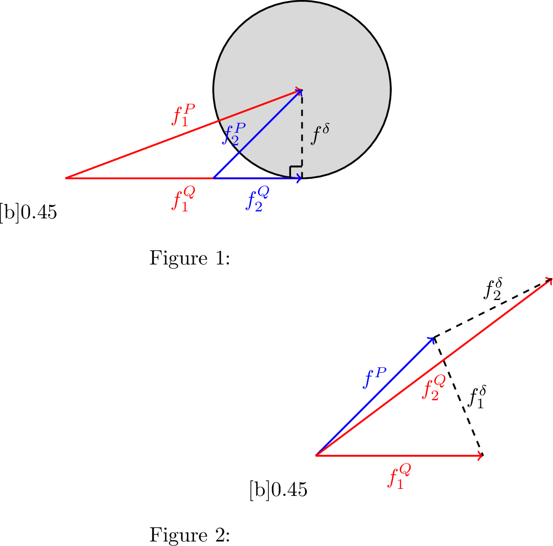
Suppose there are two source and target distribution pairs \((P_{1},Q_{1})\) and \((P_{2},Q_{2})\) with same \(m_{P}\), \(m_{\delta}\) and \(f^{\delta}\) but different \(f^{P}\) (and thus \(f^{Q}\)); see Figure 2. Despite having the same offset, the two pairs of \(f^{P}\) and \(f^{Q}\) exhibit different angels \(\theta_{1} = \arcsin( \frac{\|f^{\delta}\|_{H^{m_{\delta}}}}{\|f_{1}^{P}\|_{H^{m_{P}}}} )\) and \(\theta_{2} = \arcsin( \frac{\|f^{\delta}\|_{H^{m_{\delta}}}}{\|f_{2}^{P}\|_{H^{m_{P}}}} )\), and thus represent the different degrees of geometric similarity. While the form of \(\xi \propto \|f^{\delta}\|_{H^{m_{\delta}}}^2\) suggests two pairs have the same transfer efficiency, our upper bound indicates the pair \((P_{1}, Q_{1})\) has a higher efficiency. This aligns with the observation that \(f_{1}^{P}\) and \(f_{1}^{Q}\) are more similar since they possess a smaller geometric angle.
This example demonstrates that geometric alignment should also be a factor in explaining \(\xi\). To facilitate explaination, denote the unique corresponding element of \(f^{P}\), \(f^{Q}\) and \(f^{\delta}\) in \(L^{2}(\mathcal{X})\) as \(f^{P*}\), \(f^{Q*}\) and \(f^{\delta *}\) respectively. Then, we can express the ratio \(\xi\) as \[\xi = \frac{\|f^{P*} - f^{Q*}\|_{L^{2}}^2}{\|f^{P*}\|_{L^2}^{2}} = 1 + \frac{\|f^{Q*}\|_{L^{2}}^2}{\|f^{P*}\|_{L^{2}}^2} - 2 \frac{\|f^{Q*}\|_{L^{2}}}{\|f^{P*}\|_{L^{2}}} \cos(\angle(f^{P*}, f^{Q*})).\] This expression incorporates both angular component \(\angle(f^{P*}, f^{Q*})\) and relative magnitude component \(\frac{\|f^{Q*}\|_{L^{2}}}{\|f^{P*}\|_{L^{2}}}\) into \(\xi\). Notably, \(\xi\) is thus an unimodal function of \(\frac{\|f^{Q*}\|_{L^{2}}}{\|f^{P*}\|_{L^{2}}}\), reaching its minimum at \(1\), and also a monotonically increasing function of \(\angle(f^{P*}, f^{Q*})\). This means that if the signal strength of \(f^{P*}\) and \(f^{Q*}\) are closer, and the angle between \(f^{P*}\) and \(f^{Q*}\) is smaller, the value of \(\xi\) decreases, resulting in higher transfer efficiency; see Figure [fig:32both32angle32and32distance].
The example discussed above highlights that both the relative signal strength of the target and source functions and the geometric angle between them play significant roles in determining the efficiency of offset transfer learning. This form encompasses most transfer learning algorithms that rely on biased regularization, e.g., [1], [2], [10]. The explanation becomes more complex for general model transformation functions \(G\) due to the absence of an explicit form of \(G\), making it challenging to analyze the precise factors that influence the efficiency. In such cases, we can only conclude that the efficiency depends on the signal strength ratio of \(f^{\delta}\) to \(f^{P}\), which still refines the results in previous literature that ignored or misjudged \(\xi\).
5 Numerical Illustration↩︎
This section provides several numerical simulations to validate our theoretical findings and insights in both target-only learning and hypothesis transfer learning cases.
5.1 Simulation for Spectral Algorithms↩︎
We first aim to confirm the minimax optimality of the non-adaptive and adaptive rates established in Theorems 1 and 2. Specifically, we conduct the numerical experiments in classical nonparametric regression with a single dataset, where we consider \(\mathcal{X}= [0,1]\) and the true function \(f_{0} \in H^{m}(\mathcal{X})\) for different \(m\).
We consider the following data generation procedure: \[y_{i} = f_{0}(x_{i}) + 0.5\epsilon_{i} \qquad i = 1, \cdots, n\] where \(x_{i}\) are i.i.d. samples drawn from the uniform distribution on \(\mathcal{X}\), \(\epsilon_{i}\) are i.i.d. standard Gaussian random variables, and sample size \(n=100k\) with \(k=1,2,\cdots,30\). Since the sample path of Gaussian processes (GP) with specified covariate kernels indeed lies in certain Sobolev spaces [47], we generate true functions \(f_{0}\) by setting them as sample paths that are generated from a Gaussian process with isotropic Matérn kernels \(K_{\nu}\). Based on Corollary 4.15 in [47], we set \(\nu = 2.01\) and \(\nu = 3.01\) to generate \(f_{0}\) in \(H^{2}(\mathcal{X})\) and \(H^{3}(\mathcal{X})\).
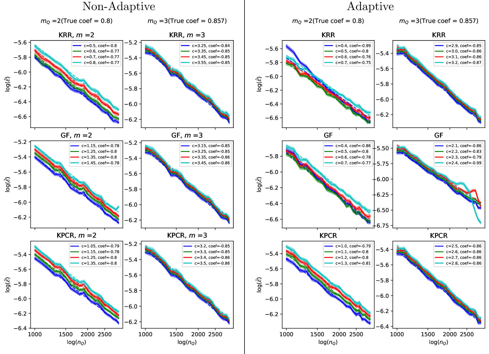
We investigate three spectral algorithms, including Kernel ridge regression (KRR), Gradient flow (GF), and Kernel principal component regression (KPCR), to recover the true regression functions. For non-adaptive rates, we set the regularization parameter \(\lambda\) as \(\lambda = \exp\{-Cn^{\frac{2}{2m + 1}}\}\) with a fixed \(C\) to construct the estimators. For adaptive rates, we set the candidate smoothness as \([1,2,\cdots,5]\) and construct the estimators through the training and validation as described in Section 3. For each combination of \(n\) and \(m\), we compute \(\hat{\mathcal{E}_{i}} = \|\hat{f} - f_{0}\|_{L_{2}}^{2}\) by Simpson’s rule with \(5000\) testing points and repeats the experiments \(100\) times. The excess risk is then approximated by \(\hat{\mathcal{E}} = \frac{1}{100}\sum_{i=1}^{100}\hat{\mathcal{E}_{i}}\). To verify the convergence rate of the error is sharp, we regress the \(\log(\hat{\mathcal{E}})\) on \(\log(n)\) and check if the regression coefficient to its theoretical counterpart \(-2m/(2m+1)\).
We test different values of \(C\) in sequence \([0.05,0.1,\cdots, 4]\), and report the optimal curve for the best choice of \(C\) in Figure 3 for non-adaptive and adaptive rates, respectively. It can be seen that the scattered points and the corresponding empirical error decay curves align with the theoretical decay curves in both non-adaptive and adaptive cases. Also, the estimated regression coefficient closely agrees with the theoretical counterparts \(-\frac{2m}{2m+1}\). Additionally, in Figure 4, the results based on different choices of \(C\) are presented, and it shows that the empirical excess risk decay rates still closely align with theoretical ones in both cases.

5.2 Simulation for Hypothesis Transfer↩︎
In this part, we present the simulation to confirm the minimax optimality of the HTL algorithm derived in Theorems 3 and 4, as well as the role of \(\xi\) as we discussed in Subsection 4.3. Specifically, we explore offset transfer learning with the data generation procedure under concept shifts defined as follows, \[\{x_{i}^{Q}\}_{i=1}^{n_{Q}}, \{x_{i}^{P}\}_{i=1}^{n_{P}} \stackrel{i.i.d.}{\sim} U([0,1]), \quad y_{i}^{P} = f^{P}(x_{i}^{P}) + 0.5 \epsilon_{i}, \quad y_{i}^{Q} = y_{i}^{P} + f^{\delta}(x_{i}^{Q}),\] where \(f^{P} \in H^{1}(\mathcal{X})\), \(f^{\delta}\in H^{2}\) or \(H^{3}\), making \(m_{P} = m_{Q} = 1\) and \(m_{\delta} = 2\) or \(3\). Throughout the simulation, we compare the excess risk of the two following learning cases.
Target-only Regression (“Target-Only”): We use KRR with Gaussian kernels to recover \(f^{Q}\) with only the target dataset \(\mathcal{D}^{Q}\). This serves as the non-transfer baseline.
Hypothesis Transfer (“Transfer”): The special HTL algorithm introduced in Subsection 4.1. To mimic practical scenarios, the pre-training phase conducts gradient methods, i.e., GF, to recover \(f^{P}\) while the fine-tuning phase uses KRR for \(f^{\delta}\).
5.2.0.1 Transfer Optimality
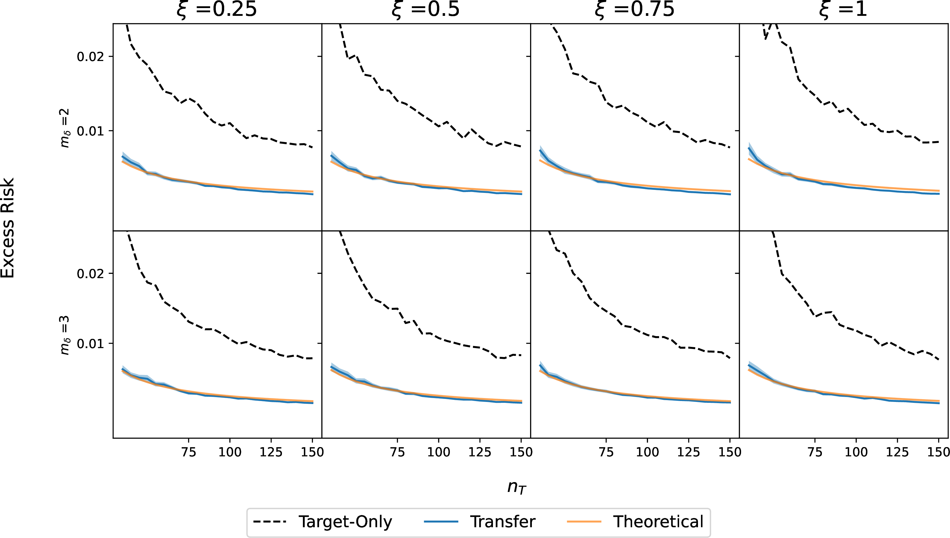
We first verify the minimax optimality. We set \(n_{P} = n_{Q}^{1.5}\) while \(n_{Q}\) varies and takes the value in \(\{40,45,\cdots,150\}\). We also manipulate the Sobolev norm of \(f^{P}\) and \(f^{\delta}\) such that the factor \(\xi\) belongs to \(\{0.25, 0.5, 0.75, 1\}\). Such settings ensure the convergence rate of excess risk for the HTL algorithm satisfies \(\|\hat{f}^{Q} - f^{Q}\|_{L^{2}}^{2} = \mathcal{O}_{\mathbb{P}}( n_{Q}^{-\frac{3m_{P}}{2m_{P}+1}} + \xi n_{Q}^{-\frac{2m_{\delta}}{2m_{\delta}+1}} ) = \mathcal{O}_{\mathbb{P}}( n_{Q}^{-1} + \xi n_{Q}^{-\frac{2m_{\delta}}{2m_{\delta}+1}} ) = \mathcal{O}_{\mathbb{P}}( n_{Q}^{-\frac{2m_{\delta}}{2m_{\delta}+1}} )\). Therefore, optimality can thus be confirmed by verifying that the empirical excess risk decay rate matches the theoretical rates \(n_{Q}^{-\frac{2m_{\delta}}{2m_{\delta}+1}}\). The excess risks under different settings are presented in Figure 5, where each curve denotes the average error over \(100\) repeated experiments. We can see the empirical excess risks of the HTL algorithm, i.e., blue ones, consistently aligned with the theoretical counterparts, i.e., orange ones, and also outperform the target-only baselines in all settings. Moreover, the excess risks for \(m_{\delta} = 3\) are lower and decay faster than those for \(m_{\delta} = 2\), which aligned with the theoretical indications. These results justify the optimality of the HTL algorithm we derived in Section 4.
5.2.0.2 Influence of \(\xi\) on Transfer Efficiency
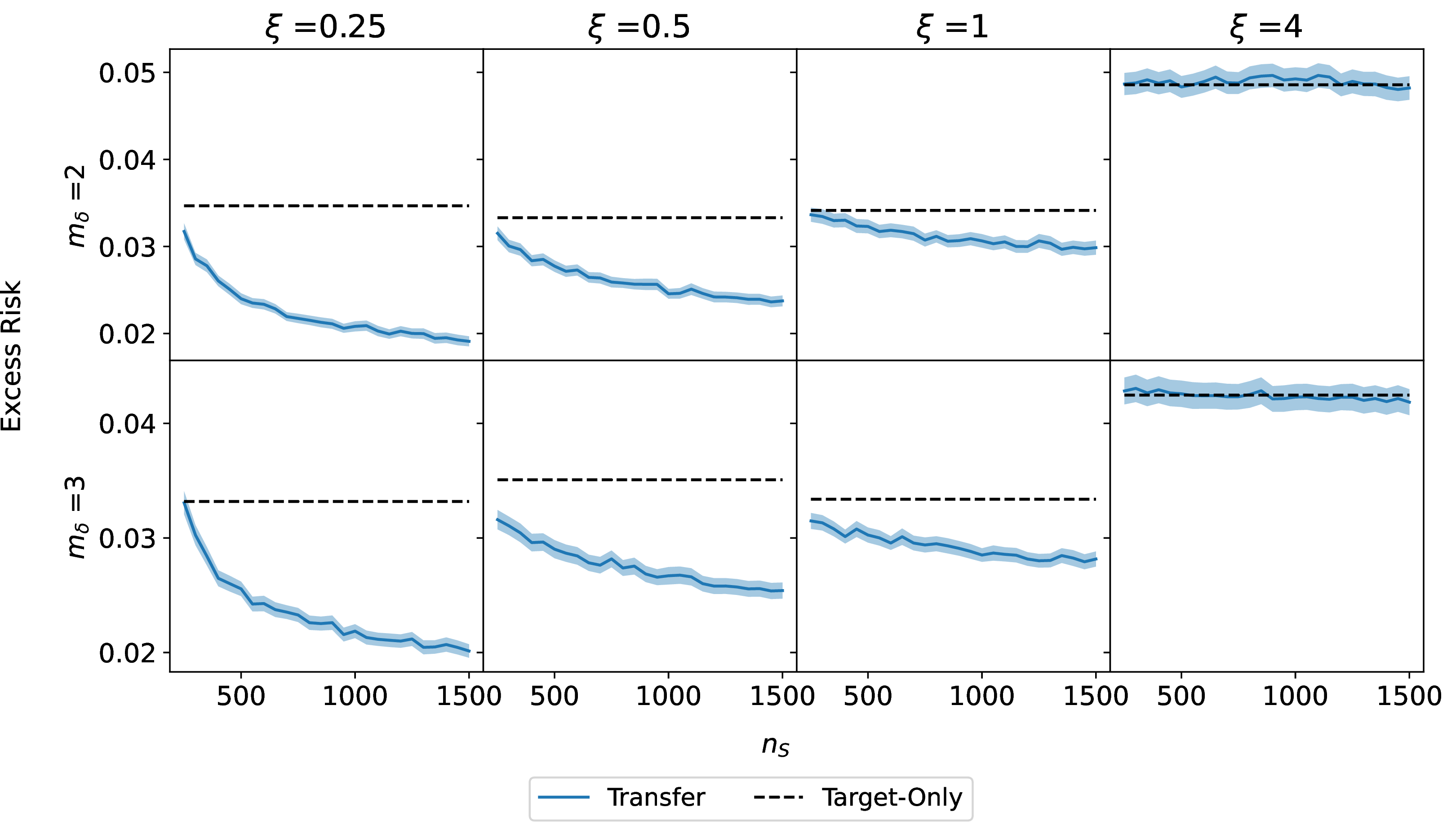
As discussed in Subsection 4.3, the magnitude of \(\xi\) affects the transfer efficiency. To confirm such influence of \(\xi\), we fix \(n_{Q} = 200\) while varying \(n_{P}\) from \(200\) to \(1500\) and \(\xi\) takes values in \(\{0.25, 0.5, 1, 4\}\). Under such settings, it is expected that as \(\xi\) increases, the fine-tuning error will start to dominate and remain unchanged, even as \(n_{P}\) increases. The results, presented in Figrue 6, show that the degree of decrease in the excess risks of the HTL algorithm diminishes as \(\xi\) increases. Eventually, these error curves become horizontal; that is, it does not decrease with the increase of \(n_{P}\). These observations confirm the influence of \(\xi\) discussed in Subsection 4.3.
6 Related Work↩︎
6.1 Hypothesis Transfer Learning↩︎
Under plausible distribution shifts relating two domains, the technique of leveraging data from source domains to enhance learnability in the target domain is known as transfer learning or domain adaptation [48], [49]. There is a long list of works on these topics in nonparametric methods and RKHS context, covering scenarios such as covariate shift [8], [50], [51], and concept shift [3], [5], [19], [52], to name a few. Focusing on transfer learning under concept shifts, the methodology of HTL has been theoretically studied over the past decade. [1], [53] studied the shifted offset being a linear model and established generalization bounds through Rademacher complexity. [13] further assumed true source functions in a Sobolev ellipsoid while shifted offsets belong to smoother ones, modeling them with finite basis functions. [5] proposed using general transformations to model domain shift and offer upper bounds on excess risk. More recently, following this transformation framework, [6] derived the optimal model transformation functions under square loss. These works, however, investigated neither the minimax optimality nor the robustness to model misspecification of HTL.
Recently, a line of work has been devoted to studying the minimax optimality for a special case of HTL, offset transfer learning, which typically involves regularizing the difference between target and pre-trained models via different norms. To name a few: [10], [12] considered \(\ell^{1}\)-norm for high-dimensional (generalized) linear regression. [54] considered \(\ell^{2}\)-norm for linear models in feature learning setting. [14] utilized RKHS-norm for functional linear models. Other similar studies for more specific problems include linear regression [45], binary classification [7], [11], [55], Gaussian mixture model [56], graphical model [57] and among others.
For theoretical studies of transfer learning on robustness against model misspecification, most works are concentrated on semiparametric models due to the fact that parametric parts are sensitive to misspecified models and can affect the efficiency of the estimator. For example, [58] utilized model averaging to achieve asymptotic minimax optimality when the target model is misspecified. Another line of works [59]–[62] developed robustness estimation procedures under the covariate shift assumption, allowing for one or multiple specified models are misspecified. For RKHS-based nonparametric regression, [29] achieved optimal HTL using misspecified kernels, but their framework was confined to offset transfer learning with the learning algorithms in both phrases being KRR. For nonparametric classification, multiple works obtained minimax optimal guarantees by using robust models, such as decision trees [44] or nearest neighbors estimators [9], under the assumption that true classification functions reside in certain Hölder spaces. Despite the distinctions in the problem setting and estimation procedures, the messages in these researches are analogous to ours: achieving robustness to model misspecification and adaptivity while ensuring minimax optimality is crucial for transfer learning algorithms, as these properties underpin their performance guarantees.
6.2 Misspecified Spectral Algorithm↩︎
For misspecified spectral algorithms, a line of works [15], [16], [34], [63]–[68] has investigated the cases where the true function belongs to the interpolation space of the RKHS associated with the imposed kernel, i.e., \([\mathcal{H}]^{s}\), and derive the minimax optimal rate for spectral algorithms under different norms. To our knowledge, the state-of-the-art results in [30] recovered the minimax optimal rate for all spectral algorithms under the \([\mathcal{H}]^{\gamma}\)-norm while removing the \(L^{\infty}(\mathcal{X})\) boundedness assumption on the true function \(f_{0}\) in previous literature. [69] further extended the results to the vector-valued spectral algorithms. Most of the aforementioned works typically assumed the eigenvalue decay rate of the imposed kernel is polynomial or the effective dimension bounded by \(\lambda^{-\beta}\). However, eigenvalues of Gaussian kernels decay exponentially fast and do not fit these assumptions. The closest case to our work is Assumption 8 in [70], which assumes a logarithmic decay of the effective dimension. Yet, this is only proven in specific instances, such as the univariate Gaussian kernel \(K(x,y) = xy + \exp\{-8(x-y)^2\}\), which is not the classical multivariate Gaussian kernel \(\exp\{-\|x-y\|_{2}^2/2h^{2}\}\) we consider.
When the imposed kernels are variable bandwidth Gaussian kernels, [43] proved that allowing regularization parameters and the bandwidths to decay polynomially yields convergence rates that can be arbitrarily close to the optimal rate in KRR when \(f_{0}\) belongs to Sobolev or Besov spaces. Later, [44] further improved the convergence rate up to logarithmic factors under the DIM condition.
Regarding the saturation effect, especially for KRR, was observed in practice and reported in [18], [33]. It was only recently that the saturation effect on KRR was theoretically proved by [71] and later extended to spectral algorithms [38]. In other specific settings, like (stochastic) distributed-based, online-based spectral algorithms and average gradient descent, the saturation effect was also noted and overcome by method-specified techniques [35], [72], [73]. Note that this does not weaken the novelty of our results since employing fixed bandwidth Gaussian kernels offers a consistent and robust solution to avoiding the potential saturation effect in arbitrary spectral algorithms with finite qualification.
7 Conclusion and Discussion↩︎
In this work, we address the underexplored problem of achieving robustness against model misspecification in hypothesis transfer learning under the concept shift condition. We first show that in classical nonparametric regression, where true functions belong to Sobolev spaces, specifying the hypothesis space as the RKHS of a fixed bandwidth Gaussian kernel allows spectral algorithms to produce estimators that attain minimax optimal convergence rates, provided the regularization parameter decays exponentially. This provides a stronger, robust result for the misspecified spectral algorithms as it can help to overcome the well-known saturation effect. Leveraging this result, we show that a modified version of a class of hypothesis transfer learning algorithms is robust against model misspecification while still attaining minimax optimality. The derived convergence rates reveal several factors that affect the transfer efficiency, which have been overlooked by previous research, and these findings are empirically validated through numerical simulations.
We aspire this work serves as a starting point for advancing robust transfer learning with statistical guarantees: it encourages the researchers to be aware of the necessity of robustness in learning algorithms under distribution shifts, particularly when leveraging conventional statistical tools or models for which misspecification is not the central research theme.
Moreover, we provide the following potential directions for further improvements. This work considers the setting where the distributions of \(X\) stay the same while conditional distributions of \(Y|X\) can vary. However, in practice, the invariant marginal distribution condition is often unverifiable, and the performance of HTL can degrade significantly when the support or covariate distributions differ substantially between domains. Exploring modifications to the HTL framework that enhance its robustness to covariate shifts while providing theoretical guarantees represents an important avenue for further study. Such advancements would significantly expand the applicability of our results.
8 Proofs for Section 3↩︎
While we introduce and present the results using the target dataset \(\mathcal{D}^{Q}\), for simplicity of notation, we present the proof in the context of classical nonparametric regression setting, i.e. \[y_{i} = f_{0}(x_{i}) + \epsilon_{i}, \quad \forall n = 1,\cdots,n,\] where the true function \(f_{0}\in H^{m_{0}}(\mathcal{X})\), and \(\epsilon_{i}\) satisfies Assumption 3. Note that replacing \(f_{0}\), \(m_{0}\) and the dataset \(\{(x_{i}, y_{i})\}_{i=1}^{n}\) with \(f^{Q}\), \(m_{Q}\) and \(\mathcal{D}^{Q}\) recovers what we presented in Section 3. Besides the notations defined in Section 2, we denote the operator norm of a bounded linear operator as \(\|\cdot\|_{op}\) and denote the effective dimension of \(T_{K}\) as \(\mathcal{N}(\lambda) =tr( (T_{K} + \lambda \mathbf{I})^{-1} T_{K} )\).
8.1 Proof of Theorem 1↩︎
The proof of the non-adaptive rate is mainly consistent with approximation-estimation error decomposition and control of each of them, respectively. We first state the approximation-estimation error decomposition. The estimator of spectral algorithms can be written as \[\hat{f} = \phi_{\lambda}(T_{K,n}) g_{n}.\] Then, we decompose the excess risk into approximation error and estimation error, i.e. \[\underbrace{\left\| \hat{f} - f_{0} \right\|_{L_{2}} }_{\text{excess risk of \hat{f}}} \leq \underbrace{\left\| \hat{f} - f_{\lambda} \right\|_{L_{2}}}_{\text{estimation error}} + \underbrace{\left\| f_{\lambda} - f_{0} \right\|_{L_{2}}}_{\text{approximation error}},\] where the intermediate term \(f_{\lambda}\) is defined as follows, \[f_{\lambda} = \phi_{\lambda}(T_{K}) T_{K}(f_{0})= \phi_{\lambda}(T_{K}) g.\] To prove the upper bound, we also need the following technical assumption.
Assumption 4. Suppose the following condition holds for some positive constants \(E_{K}\), \[\sup_{x\in \mathcal{X}} \sum_{j=1}^{\infty}\frac{s_{j}}{s_{j}+\lambda} e_{j}^{2}(x) \leq E_{K}^{2} \mathcal{N}(\lambda).\]
Remark 4. This assumption naturally holds if Gaussian integral operator \(T_{K}\) has uniformly bounded eigenfunctions, i.e., there exists a constant \(E_{K}\) such that the eigenfunction of \(T_{K}\) is uniformly bounded for all \(j \geq 1\), i.e. \(\sup_{j\geq 1}\|e_{j}\|_{L_{\infty}}\leq E_{K}\). Although the uniform boundedness condition holds for Gaussian kernels has been conjectured to be true for decades and used in research, rigorous proof still lacks and is a long-standing mathematical problem. Therefore, we consider this weaker assumption as the uniform boundedness condition for Gaussian kernels is currently out of the scope of this paper.
We now start to control each error separately. The following two theorems are used. We refer their proofs to Appendix 8.3.
Theorem 5 (Approximation error). Suppose \(f_{\lambda}\) is defined as \(f_{\lambda} = \phi_{\lambda}(T_{K}) T_{K}(f_{0})\). Then, the following inequality holds, \[\| f_{\lambda} - f_{0} \|_{L_{2}}^{2} \leq C log\left(\frac{1}{\lambda}\right)^{-m_{0}} \| f_{0} \|_{H^{m_{0}}}^{2},\] where \(C\) is a constant.
Theorem 6 (Estimation error). Suppose Assumptions 2 and 3 hold and \(\|f_{0}\|_{L_{q}}\leq C_{q}\) for some \(q\). Then by choosing \(\log(1/\lambda)\asymp n^{\frac{2}{2m_{0}+d}}\), for any fixed \(\delta \in (0,1)\), when \(n\) is sufficient large, with probability \(1-\delta\), we have \[\left \| \hat{f} - f_{\lambda} \right\|_{L_{2}} \leq C \log\left(\frac{4}{\delta}\right) n^{-\frac{m_{0}}{2m_{0}+d}}\] where \(C\) is a constant proportional to \(\sigma\).
Remark 5. Regarding the approximation error, as we mentioned in Section 3.3, the intermediate term \(f_{\lambda}\) is placed in \([H^{m_{0}}]^{s}\) while the true function in \(H^{m_{0}}\) (here, \(s\) denotes the interpolation index) for classical misspecified kernel methods. This allows one to expand \(f_{\lambda}\) and \(f_{0}\) under the same basis and makes the optimal order of \(\lambda\) in \(n\) takes polynomial pattern like Proposition 1. This technique is widely used in many misspecified kernel literature like Theorem A.2 in [30] etc. However, in our case, the intermediate term, \(f_{\lambda}\), lies in the RKHS associated with Gaussian kernels (\(s\) needs to be \(\infty\)). Therefore, the previous technique is no longer feasible. Therefore, the techniques we used are the Fourier transform of the Gaussian kernel and the Plancherel Theorem.
Regarding the estimation error, we apply standard integral operator techniques from [46], following a strategy similar to [16], [30]. Unlike most existing work focusing on polynomial eigenvalue decay, we refine the proof to address the Gaussian kernel case, where the eigenvalues decay exponentially.
Proof of Theorem 1. For approximation error, applying Theorem 5 leads to \[\|f_{\lambda} - f_{0}\|_{L_{2}}^{2} \leq C_{1} log(\frac{1}{\lambda})^{-m_{0}} \|f_{0}\|_{H^{m_{0}}}^{2}.\] Then selecting \(\log(1/\lambda) \asymp n^{\frac{2}{2m_{0}+d}}\) leads to \[\|f_{\lambda} - f_{0}\|_{L_{2}}^{2} \leq C_{1} n^{-\frac{2m_{0}}{2m_{0}+d}} \|f_{0}\|_{H^{m_{0}}}^{2}.\] For estimation error, applying Theorem 6 provides, with probability \(1-\delta\), \[\left \| \hat{f} - f_{\lambda} \right\|_{L_{2}}^{2} \leq C_{2} \left(\log \frac{4}{\delta} \right)^{2} n^{-\frac{2m_{0}}{2m_{0}+d}}.\] Combining both results finishes the proof, i.e., we have \[\left \| \hat{f} - f_{0} \right\|_{L_{2}}^{2} \leq C_{3} \left(\log \frac{4}{\delta} \right)^{2} n^{-\frac{2m_{0}}{2m_{0}+d}},\] with probability \(1-\delta\), and \(C_{3} \propto \sigma^{2} + \|f_{0}\|_{H^{m_{0}}}^{2}\) ◻
8.2 Proof of Theorem 2↩︎
Proof. To simplify the notation, for a given smoothness \(m\) and sample size \(n\), we define \[\psi_{n}(m) = \left( \frac{n}{\log n} \right)^{-\frac{2m}{2m + d}}.\] First, we show that it is sufficient to consider the true Sobolev smoothness \(m_{0}\) in the finite candidate set \(\mathcal{A}= \{m_{1},\cdots, m_{N}\}\) with \(m_{j} - m_{j-1}\asymp 1/\log n\). If \(m_{0} \in (m_{j-1}, m_{j})\), then by the embedding of Sobolev spaces, we have \(H^{m_{j}} \subset H^{m_{0}} \subset H^{m_{j-1}}\). Therefore, since \(\psi_{n}(m_{0})\) is squeezed between \(\psi_{n}(m_{j-1})\) and \(\psi_{n}(m_{j})\), it remains to show \(\psi_{n}(m_{j-1}) \asymp \psi_{n}(m_{j})\). By the definition of \(\psi_{n}(m)\), the claim follows since \[\log \frac{\psi_{n}(m_{j-1})}{\psi_{n}(m_{j})} = \left( -\frac{2m_{j-1}}{2m_{j-1}+d} + \frac{2m_{j}}{2m_{j} + d} \right) \log \frac{n}{\log n} \asymp (m_{j} - m_{j-1})\log n\asymp 1.\] Therefore, we can safely assume \(f_{0} \in H^{m_{i}}\) where \(i\in \{1,2,\cdots,N\}\).
Let \(m = \lfloor \frac{n}{2} + 1 \rfloor\), i.e. \(m\geq \frac{n}{2}\), by Theorem 1, for some constants \(C\) that doesn’t depend on \(n\), we have \[\label{eqn:32eqn132in32adaptive32estimator32via32TV} \begin{align} \left\| \hat{f}_{\lambda_{m},\mathcal{D}_{1}} - f_{0} \right\|_{L^{2}}^{2} & \leq \left( \log\frac{4}{\delta} \right)^2 \left( \text{E}(\lambda_{m},m) + \text{A}(\lambda_{m},m) \right)\\ \end{align}\tag{2}\] for all \(m \in \mathcal{A}\) simultaneously with probability at least \(1 - N \delta\). Here, \(\text{E}(\lambda,n)\) and \(\text{A}(\lambda,n)\) denote the estimation and approximation error that depends on the regularization parameter \(\lambda\) and sample size \(n\) in non-adaptive rate proof.
Furthermore, by Theorem 7.2 in [41] and Assumption 3, we have \[\label{eqn:32eqn232in32adaptive32estimator32via32TV} \begin{align} \left\|\hat{f}_{\hat{\lambda}} - f_{0} \right\|_{L^{2}}^{2} & < 6 \left( \inf_{m \in \mathcal{A}} \left\|\hat{f}_{\lambda_{m}} - f_{0} \right\|_{L^{2}}^{2} \right) + \frac{128\sigma^{2}L^2 \left(\log\frac{1}{\delta} + \log(1 + N)\right)}{n-m}\\ & < 6 \left( \inf_{m \in \mathcal{A}} \left\|\hat{f}_{\lambda_{m}} - f_{0} \right\|_{L^{2}}^{2} \right) + \frac{512 \sigma^{2}L^2 \left(\log\frac{1}{\delta} + \log(1 + N)\right)}{n} \end{align}\tag{3}\] with probability \(1 - \delta\), where the last inequality is based on the fact that \(n-m \geq \frac{n}{2} - 1 \geq \frac{n}{4}\).
Combining (2 ) and (3 ), we have \[\begin{align} \left\|\hat{f}_{\hat{\lambda}} - f_{0} \right\|_{L^{2}}^{2} & < 6 \left( \log\frac{4}{\delta} \right)^2 \left( \inf_{m \in \mathcal{A}} \text{E}(\lambda_{m},m) + \text{A}(\lambda_{m},m) \right) + \frac{512 \sigma^{2}L^2 \left(\log\frac{1}{\delta} + \log(1 + N)\right)}{n} \\ & \leq 6 C \left( \log\frac{4}{\delta} \right)^2 m^{-\frac{2m_{0}}{2m_{0} + d}} + \frac{512 \sigma^{2}L^2 \left(\log\frac{1}{\delta} + \log(1 + N)\right)}{n} \\ & \leq 12 C \left( \log\frac{4}{\delta} \right)^2 n^{-\frac{2m_{0}}{2m_{0} + d}} + \frac{512 \sigma^{2}L^2 \left(\log\frac{1}{\delta} + \log(1 + N)\right)}{n} \\ \end{align}\] with probability at least \(1 - (1+N)\delta\). With a variable transformation, we have \[\label{eqn:32eqn332in32adaptive32estimator32via32TV} \left\|\hat{f}_{\hat{\lambda}} - f_{0} \right\|_{L^{2}}^{2} \leq 12 C \left( \log\frac{4(1+N)}{\delta} \right)^2 n^{-\frac{2m_{0}}{2m_{0} + d}} + \frac{512 \sigma^{2}L^2 \left(\log\frac{1+N}{\delta} + \log(1 + N)\right)}{n}\tag{4}\] with probability \(1-\delta\). Therefore, for the first term \[\label{eqn:32eqn432in32adaptive32estimator32via32TV} \begin{align} 12 C \left( \log\frac{4(1+N)}{\delta} \right)^2 n^{-\frac{2m_{0}}{2m_{0} + d}} & \leq 24C \left\{\left(\log\frac{4}{\delta} \right)^2 \log^{2}(1+N) + 1 \right\}n^{-\frac{2m_{0}}{2m_{0} + d}} \\ & \leq 24C' \left(\log\frac{4}{\delta} \right)^2 \left( \frac{n}{\log n}\right)^{-\frac{2m_{0}}{2m_{0} + d}} + 24 C n^{-\frac{2m_{0}}{2m_{0} + d}} \end{align}\tag{5}\] where the first inequality is based on the fact that \(a+b<ab+1\) for \(a,b>1\), while the second inequality is based on the fact that \(\log(x) \leq x^{\frac{m_{0}}{2m_{0} + d}}\) for some \(n\) such that \(\log(\log n) / \log n< 1/4\). For the second term, \[\label{eqn:32eqn532in32adaptive32estimator32via32TV} \begin{align} \frac{512 \sigma^{2}L^2 \left(\log\frac{1+N}{\delta} + \log(1 + N)\right)}{n} & \leq \frac{512 \sigma^{2}L^2 \left(\log\frac{1}{\delta} + 1 + 2\log(1 + N)\right)}{n} \\ &\leq \frac{512 \sigma^{2}L^2 \left(\log\frac{1}{\delta} + 1 + 2\log n\right)}{n} \end{align}\tag{6}\] The proof is finished by combining (4 ), (5 ) and (6 ). ◻
8.3 Proof of Supporting Theorem↩︎
Proof of Theorem 5. Since \(\mathcal{X}\) has Lipschitz boundary, there exists an extension mapping from \(L_{2}(\mathcal{X})\) to \(L_{2}(\mathbb{R}^{d})\), such that the smoothness of functions in \(L_{2}(\mathcal{X})\) get preserved. Therefore, there exist constants \(C_{1}\) and \(C_{2}\) such that for any function \(g \in H^{m_{0}}(\mathcal{X})\), there exists an extension of \(g\), \(g_{e}\in H^{m_{0}}(\mathbb{R}^{d})\) satisfying \[C_{1} \|g_{e}\|_{H^{m_{0}}(\mathbb{R}^{d})} \leq \|g\|_{H^{m_{0}}(\mathcal{X})} \leq C_{2} \|g_{e}\|_{H^{m_{0}}(\mathbb{R}^{d})}.\] Denote \(f_{\lambda,e}\) as the extension of \(f_{\lambda}\), then we have \[\label{equ:32bias32proof32eqn321} \left\| f_{\lambda} - f_{0} \right\|_{L_{2}(\mathcal{X})}^{2} \leq \left\| f_{\lambda, e}|_{\mathcal{X}} - f_{0} \right\|_{L_{2}(\mathcal{X})}^{2} \leq C_{2} \left( \left\| f_{\lambda,e} - f_{0,e} \right\|_{L_{2}(\mathbb{R}^{d})}^{2} \right).\tag{7}\] where \(f_{\lambda,e}|_{\mathcal{X}}\) is the restriction of \(f_{\lambda,e}\) on \(\mathcal{X}\). By Fourier transform of the Gaussian kernel and Plancherel Theorem, we have \[\begin{align}\label{equ:32bias32proof32eqn322} & \left\|f_{\lambda, e}-f_{0,e}\right\|_{L_2(\mathbb{R}^{d})}^2 \\ = & \int_{\mathbb{R}^{d}}\left|\mathcal{F}\left(f_{0,e}\right)(\omega)-\mathcal{F}\left(f_{\lambda, e}\right)(\omega)\right|^2 d \omega \\ = & \int_{\mathbb{R}^{d}} |\mathcal{F}\left(f_{0,e}\right)(\omega)|^2 \big[ 1 - \phi_{\lambda}\left( \mathcal{F}(K)(\omega) \right) \mathcal{F}(K)(\omega) \big]^2 d \omega \\ \leq & C_{3}\int_{\mathbb{R}^{d}} \lambda \exp\left\{C\|\omega\|_{2}^{2}\right\} |\mathcal{F}\left(f_{0,e}\right)(\omega)|^2 d \omega \\ \leq & C_{3} \int_{\mathbb{R}^{d}} \lambda \exp\left\{C(1+\|\omega\|_{2}^{2})\right\} |\mathcal{F}\left(f_{0,e}\right)(\omega)|^2 d \omega \end{align}\tag{8}\] where \(\mathcal{F}(K) = \exp\{-C\|\omega\|^2\}\) is the Fourier transform of the Gaussian kernel, and the first equality is based on the property of filter function with \(\beta = 0.5\). To apply the property of the filter function, we also need to verify the Fourier transform of the Gaussian kernel ranges from \(0\) to \(\kappa^2\). For \(x,x^{'} \in \mathcal{X}\), let \(\xi = \|x - x^{'}\|\) denote the Euclidean distance between \(x\) and \(x'\), then for \(\omega \in \mathbb{R}\) \[\begin{align} \mathcal{F}(K)(\omega) & = \frac{1}{(\sqrt{2\pi})^{d}} \int_{\mathbb{R}^{d}} \exp\left\{- \frac{\xi^2}{\gamma}\right\} \exp\left\{-i \omega \xi\right\} d\xi \\ & = \frac{1}{(\sqrt{2\pi})^{d}} \prod_{j=1}^{d} \int_{\mathbb{R}} \exp\left\{- \frac{\xi_{j}^2}{\gamma}\right\} \exp\left\{-i \omega_{j} \xi_{j}\right\} d\xi_{j} \\ & = \frac{1}{(\sqrt{2\pi})^{d}} \prod_{j=1}^{d} \int_{\mathbb{R}} \exp\left\{- \frac{\xi_{j}^2}{\gamma}\right\} \cos\left( \omega_{j} \xi_{j} \right) d\xi_{j} \\ & \leq \left(\sqrt{\frac{2}{\pi}}\right)^{d}\prod_{j=1}^{d} \int_{\mathbb{R}^{+}} \cos\left( \omega_{j} \xi_{j} \right) d\xi_{j} \\ & \leq \left(\sqrt{\frac{2}{\pi}}\right)^{d} \leq 1 \leq \kappa^{2} \end{align}\] where the last inequality is based on the fact that \(\sup_{x}K(x,x)\leq 1\) for Gaussian kernels.
Define \(\Omega= \{ \omega : \lambda exp\{C(1+\|\omega\|_{2}^{2})\} <1 \}\) and \(\Omega^{C} = \mathbb{R}^{d} \backslash \Omega\). Notice over \(\Omega^{C}\), we have \[(1+\|\omega\|_{2}^{2}) \geq \frac{1}{C}log\left( \frac{1}{\lambda} \right) \implies C^{m_{0}} log\left( \frac{1}{\lambda} \right)^{-m_{0}} (1+\|\omega\|_{2}^{2})^{m_{0}} \geq 1.\] Besides, over \(\Omega\), we first note that the function \(h(\omega) = exp\{ C(1+\|\omega\|_{2}^{2})\} / (1+\|\omega\|_{2}^{2})^{m_{0}}\) reaches its maximum \(C^{m_{0}} \lambda^{-1} log(\frac{1}{\lambda})^{-m_{0}}\) if \(\lambda\) satisfies \(\lambda < exp\{-m_{0}\}\) and \(\lambda log(\frac{1}{\lambda})^{m_{0}} \leq C^{m_{0}} exp\{-C\}\). One can verify when \(\lambda \rightarrow 0\) as \(n\rightarrow 0\), the two previous inequality holds. Then \[\lambda exp\{C(1+\|\omega\|_{2}^{2})\} \leq C^{m_{0}} log\left( \frac{1}{\lambda} \right)^{-m_{0}} (1+\|\omega\|_{2}^{2})^{m_{0}} \quad \forall \omega \in \Omega.\] Combining the inequality over \(\Omega\) and \(\Omega^{C}\), \[\begin{align}\label{equ:32bias32proof32eqn323} & \int_{\mathbb{R}^{d}} \lambda \exp\{C(1+\|\omega\|_{2}^{2})\} |\mathcal{F}\left(f_{0,e}\right)(\omega)|^2 d \omega \\ \leq & \int_{\Omega} \lambda \exp\{C(1+\|\omega\|_{2}^{2})\} |\mathcal{F}\left(f_{0,e}\right)(\omega)|^2 d \omega + \int_{\Omega^{C}} |\mathcal{F}\left(f_{0,e}\right)(\omega)|^2 d \omega \\ \leq & C^{m_{0}} log\left( \frac{1}{\lambda} \right)^{-m_{0}} \int_{\mathbb{R}^{d}} (1+\|\omega\|_{2}^{2})^{m_{0}} |\mathcal{F}(f_{0,e})(\omega)|^2 d \omega \\ = & C^{m_{0}} log\left( \frac{1}{\lambda} \right)^{-m_{0}} \|f_{0,e}\|_{H^{m_{0}}(\mathbb{R}^{d})}^{2} \\ \leq & C^{'} log\left( \frac{1}{\lambda} \right)^{-m_{0}} \|f_{0}\|_{H^{m_{0}}(\mathcal{X})}^{2}. \end{align}\tag{9}\] Combining the inequality (7 ), (8 ), and (9 ), we have \[\|f_{\lambda} - f_{0}\|_{L_{2}(\mathcal{X})}^2 \leq C' log\left( \frac{1}{\lambda} \right)^{-m_{0}} \|f_{0}\|_{H^{m_{0}}(\mathcal{X})}^{2}.\] for some constant \(C'\), which completes the proof. ◻
Proof of Theorem 6. First, decompose the estimation error as \[\begin{align} \left\| \hat{f} - f_{\lambda} \right\|_{L_{2}} & = \left\| T_{K}^{\frac{1}{2}} \left( \hat{f} - f_{\lambda} \right) \right\|_{\mathcal{H}_{K}} \\ & \leq \underbrace{\left\|T_{K}^{\frac{1}{2}} \left( T_{K} + \lambda I \right)^{-\frac{1}{2}} \right\|_{op}}_{A_{1}} \cdot \underbrace{\left\| \left( T_{K} + \lambda I \right)^{\frac{1}{2}} \left( T_{K,n} + \lambda I \right)^{-\frac{1}{2}} \right\|_{op}}_{A_{2}} \\ & \quad \cdot \underbrace{\left\| \left( T_{K,n} + \lambda I \right)^{\frac{1}{2}} \left( \hat{f} - f_{\lambda} \right) \right\|_{\mathcal{H}_{K}}}_{A_{3}} \end{align}\] For the first term \(A_{1}\), we have \[A_{1} = \left\|T_{K}^{\frac{1}{2}} \left( T_{K} + \lambda I \right)^{-\frac{1}{2}} \right\|_{op} = \sup_{i\geq 1} \left( \frac{s_{j}}{s_{j} + \lambda}\right)^{\frac{1}{2}} \leq 1.\] For the second term \(A_{2}\), using Lemma 2 with sufficient large \(n\), we have \[u:=\frac{\mathcal{N}(\lambda)}{n} \log ( \frac{8\mathcal{N}(\lambda)}{\delta} \frac{(\|T_{K}\|_{op}+\lambda)}{\|T_{K}\|_{op}}) \leq \frac{1}{8}\] such that \[\left\| \left( T_{K} + \lambda I \right)^{-\frac{1}{2}} \left( T_{K} - T_{K,n} \right) \left( T_{K} + \lambda I \right)^{-\frac{1}{2}} \right\|_{op} \leq \frac{4}{3}u + \sqrt{2u}\leq \frac{2}{3}\] holds with probability \(1-\frac{\delta}{2}\). Thus, \[\begin{align} A_{2}^{2} &= \left\| (T_{K} + \lambda I)^{\frac{1}{2}} (T_{K,n} + \lambda I)^{-\frac{1}{2}}\right\|_{op}^2 \\ & = \left\| (T_{K} + \lambda I)^{\frac{1}{2}} (T_{K,n} + \lambda I)^{-1} (T_{K} + \lambda I )^{\frac{1}{2}}\right\|_{op}\\ & =\left\|\left( (T_{K} + \lambda I)^{-\frac{1}{2}}\left(T_{K,n}+\lambda\right) (T_{K} + \lambda I) ^{-\frac{1}{2}}\right)^{-1}\right\|_{op} \\ & =\left\|\left(I- (T_{K} + \lambda I )^{-\frac{1}{2}}\left(T_{K,n}-T_{K}\right) (T_{K} + \lambda I )^{-\frac{1}{2}}\right)^{-1}\right\|_{op} \\ & \leq \sum_{k=0}^{\infty}\left\| (T_{K} + \lambda I )^{-\frac{1}{2}}\left(T_{K} - T_{K,n}\right) (T_{K} + \lambda I )^{-\frac{1}{2}}\right\|_{op}^k \\ & \leq \sum_{k=0}^{\infty}\left(\frac{2}{3}\right)^k \leq 3, \end{align}\] For the third term \(A_{3}\), notice \[\hat{f} - f_{\lambda} = \phi_{\lambda}(T_{K,n})\left[ g_{n} - T_{K,n}(f_{\lambda}) \right] - \psi_{\lambda}(T_{K,n})(f_{\lambda})\] where \(\psi_{\lambda}(z) = 1 - z\phi_{\lambda}(z)\). Therefore, \[\begin{align} A_{3} & = \left\| \left( T_{K,n} + \lambda I \right)^{\frac{1}{2}} \left[ \hat{f} - f_{\lambda} \right] \right\|_{\mathcal{H}_{K}} \\ & \leq \underbrace{ \left\| \left( T_{K,n} + \lambda I \right)^{\frac{1}{2}} \phi_{\lambda}(T_{K,n}) \left[ g_{n} - T_{K,n}(f_{\lambda}) \right] \right\|_{\mathcal{H}_{K}}}_{A_{31}} + \underbrace{\left\| \left( T_{K,n} + \lambda I \right)^{\frac{1}{2}} \psi_{\lambda}(T_{K,n}) f_{\lambda} \right\|_{\mathcal{H}_{K}}}_{A_{32}} \end{align}\] For \(A_{31}\), we have \[\label{eqn:32equation32of32A9531} \begin{align} A_{31} \leq & \left\| \left( T_{K,n} + \lambda I \right)^{\frac{1}{2}} \phi_{\lambda}(T_{K,n}) \left( T_{K,n} + \lambda I \right)^{\frac{1}{2}} \right\|_{op} \cdot \left\| \left( T_{K,n} + \lambda I \right)^{-\frac{1}{2}} \left( T_{K} + \lambda I \right)^{\frac{1}{2}} \right\|_{op} \\ & \quad \cdot \left\| \left( T_{K} + \lambda I \right)^{-\frac{1}{2}} \left[ g_{n} - T_{K,n}(f_{\lambda})\right] \right\|_{\mathcal{H}_{K}} \end{align}\tag{10}\]
For the first term in (10 ), the properties of filter function indicate \(z\phi_{\lambda}(z)\leq E\) and \(\lambda \phi_{\lambda}(z)\leq E\), thus we have \[\left\| \left( T_{K,n} + \lambda I \right)^{\frac{1}{2}} \phi_{\lambda}(T_{K,n}) \left( T_{K,n} + \lambda I \right)^{\frac{1}{2}} \right\|_{op} = \left\| \left( T_{K,n} + \lambda I \right)^{1} \phi_{\lambda}(T_{K,n}) \right\|_{op} \leq 2E.\]
For the second term in (10 ), the bounds for \(A_{2}\) implies \[\left\| \left( T_{K,n} + \lambda I \right)^{-\frac{1}{2}} \left( T_{K} + \lambda I \right)^{\frac{1}{2}} \right\|_{op} \leq \sqrt{3}.\]
For the third term in (10 ), by choosing \(log(1/\lambda) \asymp n^{\frac{2}{2m_{0}+d}}\), \[\begin{align} & \left\| \left( T_{K} + \lambda I \right)^{-\frac{1}{2}} \left[ g_{n} - T_{K,n}(f_{\lambda})\right] \right\|_{\mathcal{H}_{K}} \\ & \leq \left\| \left( T_{K} + \lambda I \right)^{-\frac{1}{2}} \left[ (g_{n} - T_{K,n}(f_{\lambda})) - (g - T_{K}(f_{\lambda}))\right] \right\|_{\mathcal{H}_{K}} \\ & \qquad + \left\| \left( T_{K} + \lambda I \right)^{-\frac{1}{2}} \left[ g - T_{K}(f_{\lambda})\right] \right\|_{\mathcal{H}_{K}} \\ & \leq C \log\left(\frac{4}{\delta}\right)n^{-\frac{m_{0}}{2m_{0}+d}} + \left\| \left( T_{K} + \lambda I \right)^{-\frac{1}{2}} T_{K} \right\|_{op} \cdot \left\|f_{0} - f_{\lambda} \right\|_{L_{2}} \\ & \leq C \log\left(\frac{4}{\delta}\right)n^{-\frac{m_{0}}{2m_{0}+d}} + C^{'} n^{-\frac{m_{0}}{2m_{0}+d}} \left\| f_{0} \right\|_{H^{m_{0}}} \\ & \leq C \log\left(\frac{4}{\delta}\right)n^{-\frac{m_{0}}{2m_{0}+d}} \end{align}\] where \(\left\| \left( T_{K} + \lambda I \right)^{-\frac{1}{2}} T_{K} \right\|_{op}\leq 1\) is the same as bounding \(A_{1}\), the second inequality is based on Lemma 3, and the third inequality is based on estimation error.
Combining all results, we have \[A_{31} \leq C \log\left(\frac{4}{\delta}\right)n^{-\frac{m_{0}}{2m_{0}+d}}\] with probability \(1-\frac{\delta}{2}\).
Turning to \(A_{32}\), with the properties of filter function, we have \[\left\| \left( T_{K,n} + \lambda I \right)^{\frac{1}{2}} \psi_{\lambda}(T_{K,n})\right\|_{op} \leq \sup_{z \in\left[0, \kappa^2\right]}(z + \lambda)^{\frac{1}{2}}\psi_{\lambda}(z) \leq \sup_{z \in\left[0, \kappa^2\right]}(z^{\frac{1}{2}} + \lambda^{\frac{1}{2}})\psi_{\lambda}(z) \leq 2 F_{\tau} \lambda^{\frac{1}{2}}.\] Thus, \[\begin{align} A_{32} & \leq \left\| \left( T_{K,n} + \lambda I \right)^{\frac{1}{2}} \psi_{\lambda}(T_{K,n})\right\|_{op} \cdot \left\| \phi_{\lambda}(T_{K})T_{K}(f_0) \right\|_{\mathcal{H}_{K}} \\ & \leq 2 F_{\tau} \lambda^{\frac{1}{2}} \left\| \phi_{\lambda}(T_{K})T_{K} \right\|_{op} \left\| f_{0} \right\|_{L_{2}}\\ & \leq 2 F_{\tau} \lambda^{\frac{1}{2}} E \left\| f_{0} \right\|_{H^{m_{0}}}. \end{align}\] Notice having \(\lambda \asymp \exp\{-Cn^{\frac{2}{2m_{0}+d}}\}\), we have \(A_{32} = o(A_{31})\). Finally, combining the bounds on \(A_{1},A_{2},A_{3}\), we finish the proof. ◻
8.4 Supporting Lemmas↩︎
Lemma 2. For all \(\delta \in (0,1)\), with probability at least \(1-\delta\), we have \[\left\| \left( T_{K} + \lambda I \right)^{-\frac{1}{2}} \left( T_{K} - T_{K,n} \right) \left( T_{K} + \lambda I \right)^{-\frac{1}{2}} \right\|_{op} \leq \frac{4\mathcal{N}(\lambda)B}{3n} + \sqrt{\frac{2\mathcal{N}(\lambda)}{n}B}\] where \[B = \log \left( \frac{4\mathcal{N}(\lambda)}{\delta} \frac{(\|T_{K}\|_{op}+\lambda)}{\|T_{K}\|_{op}} \right).\]
Proof. Denote \(A_{i} = (T_{K} + \lambda I )^{-\frac{1}{2}} (T_{K} - T_{K,x_{i}}) (T_{K} + \lambda I )^{-\frac{1}{2}}\), applying Lemma 6, we get \[\begin{align} \|A_{i}\|_{op} & \leq \left\| \left( T_{K} + \lambda I \right)^{-\frac{1}{2}} T_{K,x} \left( T_{K} + \lambda I \right)^{-\frac{1}{2}}\right\|_{op} + \left\| \left( T_{K} + \lambda I \right)^{-\frac{1}{2}} T_{K,x_{i}} \left( T_{K} + \lambda I \right)^{-\frac{1}{2}}\right\|_{op} \\ & \leq 2 E_{K}^{2} \mathcal{N}(\lambda) \end{align}\] Notice \[\begin{align} \mathop{\mathrm{E}}A_{i}^2 & \preceq \mathop{\mathrm{E}}\left[ \left( T_{K} + \lambda I \right)^{-\frac{1}{2}} T_{K,x_{i}} \left( T_{K} + \lambda I \right)^{-\frac{1}{2}} \right]^2 \\ & \preceq E_{K}^{2} \mathcal{N}(\lambda ) \mathop{\mathrm{E}}\left[ \left( T_{K} + \lambda I \right)^{-\frac{1}{2}} T_{K,x_{i}} \left( T_{K} + \lambda I \right)^{-\frac{1}{2}} \right] \\ & = E_{K}^{2} \mathcal{N}(\lambda ) (T_{K} + \lambda I )^{-1}T_{K} := V \end{align}\] where \(A\preceq B\) denotes \(B-A\) is a positive semi-definite operator. Notice \[\|V\|_{op} = \mathcal{N}(\lambda) \frac{\|T_{K}\|_{op}}{\|T_{K}\|_{op} + \lambda} \leq \mathcal{N}(\lambda), \quad \text{and} \quad tr(V) = \mathcal{N}(\lambda)^2.\] The proof is finished by applying Lemma 7 to \(A_{i}\) and \(V\). ◻
Lemma 3. Suppose that Assumptions in the estimation error theorem hold. We have \[\left\| \left( T_{K} + \lambda I \right)^{-\frac{1}{2}} \left( g_{n} - \left( T_{K,n} + \lambda I \right)^{-1}f_{\lambda} \right) \right\|_{\mathcal{H}_{K}} \leq C \log\left(\frac{4}{\delta}\right) n^{-\frac{m_{0}}{2m_{0}+d}}\] where \(C\) is a universal constant.
Proof. Denote \[\begin{align} & \xi_{i} = \xi(x_i,y_i) = \left( T_{K} + \lambda I \right)^{-\frac{1}{2}}(K_{x_i}y_i - T_{K,x_i}f_{\lambda}) \\ & \xi_{x} = \xi(x,y) = \left( T_{K} + \lambda I \right)^{-\frac{1}{2}}(K_{x}y - T_{K,x}f_{\lambda}), \end{align}\] then it is equivalent to show \[\left\| \frac{1}{n}\sum_{i=1}^{n} \xi_{i} - \mathop{\mathrm{E}}\xi_{x} \right\|_{\mathcal{H}_{K}} \leq C \log\left(\frac{4}{\delta}\right) n^{-\frac{m_{0}}{2m_{0}+d}}\] Define \(\Omega_{1} = \{x\in \mathcal{X}: |f_{0}|\leq t\}\) and \(\Omega_{2} = \mathcal{X}\backslash\Omega_{1}\). We decomposite \(\xi_{i}\) and \(\xi_{x}\) over \(\Omega_{1}\) and \(\Omega_{2}\), which leads to \[\begin{align} \left\| \left( T_{K} + \lambda I \right)^{-\frac{1}{2}} \left( g_{n} - \left( T_{K,n} + \lambda I \right)^{-1}f_{\lambda} \right) \right\|_{\mathcal{H}_{K}} & \leq \underbrace{\left\|\frac{1}{n} \sum_{i=1}^n \xi_i I_{x_i \in \Omega_1}-\mathop{\mathrm{E}}\xi_x I_{x \in \Omega_1}\right\|_{\mathcal{H}_{K}}}_{B_{1}} \\ & \quad + \underbrace{\left\|\frac{1}{n} \sum_{i=1}^n \xi_i I_{x_i \in \Omega_2}\right\|_{\mathcal{H}_{K}}}_{B_{2}} + \underbrace{\left\|\mathop{\mathrm{E}}\xi_x I_{x \in \Omega_2}\right\|_{\mathcal{H}_{K}}}_{B_{3}}. \end{align}\] For \(B_{1}\), applying Lemma 4, for any \(\delta \in (0,1)\), with probability \(1-\delta\), we have \[\label{eqn:32upper32bound32for32B1} B_{1} \leq \log\left(\frac{2}{\delta}\right) \left( \frac{C_{1}\sqrt{\mathcal{N}(\lambda)}}{n} \tilde{M} + \frac{C_{2}\sqrt{\mathcal{N}(\lambda)}}{\sqrt{n}} + \frac{C_{1}log(\frac{1}{\lambda})^{-\frac{m_{0}}{2}}\sqrt{\mathcal{N}(\lambda)}}{\sqrt{n}} \right)\tag{11}\] where \(C_{1} = 8\sqrt{2}\), \(C_{2} = 8\sigma\) and \(\tilde{M} = L + (\mathcal{N}(\lambda)+1)t\). By choosing \(\lambda \asymp \exp\{ -C n^{\frac{2}{2m_{0}+d}}\}\) and applying Lemma 5, we have
for the second term in 11 , \[\frac{C_{2}\sqrt{\mathcal{N}(\lambda)}}{\sqrt{n}} \asymp n^{-\frac{m_{0}}{2m_{0}+d}}.\]
for the third term in 11 , \[\frac{C_{1}log(\frac{1}{\lambda})^{-\frac{m_{0}}{2}}\sqrt{\mathcal{N}(\lambda)}}{\sqrt{n}} \lesssim \frac{C_{2}\sqrt{\mathcal{N}(\lambda)}}{\sqrt{n}} \asymp n^{-\frac{m_{0}}{2m_{0}+d}}.\]
for the first term in 11 , \[\frac{C_{1}\sqrt{\mathcal{N}(\lambda)}}{n} \tilde{M}\leq \frac{C_1 L \sqrt{\mathcal{N}(\lambda)}}{n} + \frac{C_1 t \mathcal{N}(\lambda)^{\frac{3}{2}}}{n} \lesssim n^{-\frac{m_{0}}{2m_{0}+d}} \quad \text{given} \quad t \leq n^{\frac{2m_{0}-d}{2(2m_{0}+d)}}.\]
Combining all facts, if \(t \leq n^{\frac{2m_{0}-d}{2(2m_{0}+d)}}\), with probability \(1-\delta\) we have \[B_{1} \leq C \log\left(\frac{2}{\delta}\right) n^{-\frac{m_{0}}{2m_{0}+d}}.\] For \(B_{2}\), we have \[\begin{align} \tau_n:=P\left(B_{2}> \frac{\sqrt{\mathcal{N}(\lambda)}}{\sqrt{n}} \right) & \leq P\left(\exists x_i \text{ s.t. } x_i \in \Omega_2\right) \\ & =1-P\left(x \notin \Omega_2\right)^n \\ & =1-P\left(\left|f_{0}(x)\right| \leq t\right)^n \\ & \leq 1-\left(1-\frac{\left(C_q\right)^q}{t^q}\right)^n . \end{align}\] Letting \(\tau_{n} \rightarrow 0\) leading \(t\gg n^{\frac{1}{q}}\). That is to say, if \(t\gg n^{\frac{1}{q}}\) holds, we have \(\tau_{n} = P\left(B_{2}> B_{1} \right) \rightarrow 0\).
For \(B_{3}\), we have \[\begin{align} B_{3} & \leq \mathop{\mathrm{E}}\left\| \xi_{x}I_{x\in \Omega_{2}} \right\|_{\mathcal{H}_{K}} \\ & \leq \mathop{\mathrm{E}}\left[ \left\| (T_{K} + \lambda I)^{-\frac{1}{2}} K(x,\cdot) \right\|_{\mathcal{H}_{K}} \left| \left( y - f_{0}(x) \right)I_{x\in \Omega_{2}} \right| \right] \\ & \leq E_{K}^{2} \mathcal{N}(\lambda) \mathop{\mathrm{E}}\left| \left( y - f_{0}(x) \right)I_{x\in \Omega_{2}} \right| \\ & \leq E_{K}^{2} \mathcal{N}(\lambda) \left( \mathop{\mathrm{E}}\left| \left( f_{\lambda} - f_{0}(x) \right)I_{x\in \Omega_{2}} \right| + \mathop{\mathrm{E}}\left| \epsilon I_{x\in \Omega_{2}} \right| \right) \end{align}\] Using Cauchy-Schwarz inequality yields \[\mathop{\mathrm{E}}\left| \left( f_{\lambda} - f_{0}(x) \right)I_{x\in \Omega_{2}} \right| \leq \left\|f_{0} - f_{\lambda} \right\|_{L_{2}} P(x\in \Omega_{2}) \leq log(\frac{1}{\lambda})^{-\frac{m_{0}}{2}} (C_{q})^{q} t^{-q}\] In addition, we have \[\mathop{\mathrm{E}}\left| \epsilon I_{x\in \Omega_{2}} \right| \leq \sigma \mathop{\mathrm{E}}\left| I_{x\in \Omega_{2}} \right| \leq \sigma (C_{q})^{q} t^{-q}.\] Together, we have \[B_{3} \leq log(\frac{1}{\lambda})^{-\frac{m_{0}}{2}} (C_{q})^{q} t^{-q} + \sigma (C_{q})^{q} t^{-q}.\] Notice if we pick \(q \geq \frac{2(2m_{0}+d)}{2m_{0}-d}\), there exist \(t\) such that with probability \(1-\delta - \tau_{n}\), we have \[B_{1} + B_{2} + B_{3} \leq C \log\left(\frac{2}{\delta}\right) n^{-\frac{m_{0}}{2m_{0}+d}}.\] For fixed \(\delta\), as \(n\rightarrow\infty\), \(\tau_{n}\) is sufficiently small such that \(\tau_{n} = o(\delta)\), therefore without loss of generality, we can say with probability \(1-\delta - \tau_{n}\), we have \[B_{1} + B_{2} + B_{3} \leq C \log\left(\frac{2}{\delta}\right) n^{-\frac{m_{0}}{2m_{0}+d}}.\] ◻
Lemma 4. Under the same conditions as Lemma 3, we have \[\left\|\frac{1}{n} \sum_{i=1}^n \xi_i I_{x_i \in \Omega_1}-\mathop{\mathrm{E}}\xi_x I_{x \in \Omega_1}\right\|_{\mathcal{H}_{K}}\leq \log\left(\frac{2}{\delta}\right) \left( \frac{C_{1}\sqrt{\mathcal{N}(\lambda)}}{n} \tilde{M} + \frac{C_{2}\sqrt{\mathcal{N}(\lambda)}}{\sqrt{n}} + \frac{C_{1}log(\frac{1}{\lambda})^{-\frac{\alpha}{2}}\sqrt{\mathcal{N}(\lambda)}}{\sqrt{n}} \right)\] where \(C_{1} = 8\sqrt{2}\), \(C_{2} = 8\sigma\) and \(\tilde{M} = L + (\mathcal{N}(\lambda)+1)t\).
Proof. The objective can be typically controlled by certain concentration inequality. Therefore, to leverage Bernstein inequality, i.e., Lemma 8, we first bound the \(m\)-th moment of \(\xi_{x}I_{x\in \Omega_{1}}\). \[\begin{align} \mathop{\mathrm{E}}\left\|\xi_{x} I_{x \in \Omega_{1}}\right\|_{\mathcal{H}_{K}}^m & =\mathop{\mathrm{E}}\left\|\left( T_{K} + \lambda I \right)^{-\frac{1}{2}} K_x\left(y-f_\lambda(x)\right) I_{x \in \Omega_{1}}\right\|_{\mathcal{H}_{K}}^m \\ & \leq \mathop{\mathrm{E}}\left(\left\|\left( T_{K} + \lambda I \right)^{-\frac{1}{2}} K(x, \cdot)\right\|_{\mathcal{H}_{K}}^m \mathop{\mathrm{E}}\left(\left|\left(y-f_\lambda(x)\right) I_{x \in \Omega_{1}}\right|^m \mid x\right)\right) . \end{align}\] Using the inequality \((a+b)^m \leq 2^{m-1}\left(a^m+b^m\right)\), we have \[\begin{align} \left|y-f_\lambda(x)\right|^m & \leq 2^{m-1}\left(\left|f_\lambda(x)-f_\rho^*(x)\right|^m+\left|f_\rho^*(x)-y\right|^m\right) \\ & =2^{m-1}\left(\left|f_\lambda(x)-f_\rho^*(x)\right|^m+|\epsilon|^m\right) . \end{align}\] Combining the inequalities, we have \[\begin{align} \mathop{\mathrm{E}}\left\|\xi_{x} I_{x \in \Omega_{1}}\right\|_{\mathcal{H}_{K}}^m & \leq \underbrace{2^{m-1} \mathop{\mathrm{E}}\left(\left\|\left( T_{K} + \lambda I \right)^{-\frac{1}{2}} K(x, \cdot)\right\|_{\mathcal{H}_{K}}^m\left|\left(f_\lambda(x)-f_\rho^*(x)\right) I_{x \in \Omega_{1}}\right|^m\right)}_{C_{1}} \\ &\quad + \underbrace{2^{m-1} \mathop{\mathrm{E}}\left(\left\|\left( T_{K} + \lambda I \right)^{-\frac{1}{2}} K(x, \cdot)\right\|_{\mathcal{H}_{K}}^m \mathop{\mathrm{E}}\left(\left|\epsilon I_{x \in \Omega_{1}}\right|^m \mid x\right)\right)}_{C_{2}}. \end{align}\] We first focus on \(C_{2}\), by Lemma 6, we have \[\mathop{\mathrm{E}}\left\|\left( T_{K} + \lambda I \right)^{-\frac{1}{2}} K(x, \cdot)\right\|_{\mathcal{H}_{K}}^m \leq \left( E_{K}^{2} \mathcal{N}(\lambda) \right)^{\frac{m}{2}}.\] By the error moment assumption, we have \[\mathop{\mathrm{E}}\left(\left|\epsilon I_{x \in \Omega_{1}}\right|^m \mid x\right) \leq \mathop{\mathrm{E}}\left(\left|\epsilon \right|^m \mid x\right) \leq \frac{1}{2}m! \sigma^2 L^{m-2},\] together, we have \[\label{eqn:32bound32on32A2} C_{2} \leq \frac{1}{2} m! \left(\sqrt{2}\sigma \sqrt{\mathcal{N}(\lambda)} \right)^{2} \left(2L \mathcal{N}(\lambda)\right)^{m-2}.\tag{12}\] Turning to bounding \(C_{1}\), we first have \[\begin{align} \left\| (f_{\lambda} - f_{0})I_{x\in \Omega_{1}} \right\|_{L_{\infty}} & \leq \left\| f_{\lambda} I_{x\in \Omega_{1}} \right\|_{L_{\infty}} + \left\| f_{0} I_{x\in \Omega_{1}} \right\|_{L_{\infty}} \\ & \leq \left\| (T_{K} + \lambda I)^{-1}T_{K}(f_{0}) I_{x\in \Omega_{1}} \right\|_{L_{\infty}} + \left\| f_{0} I_{x\in \Omega_{1}} \right\|_{L_{\infty}} \\ & \leq \left( \left\| (T_{K}+\lambda I)^{-1}T_{K} \right\|_{op} + 1 \right)\left\| f_{0} I_{x\in \Omega_{1}} \right\|_{L_{\infty}}\\ & \leq \left( \mathcal{N}(\lambda) + 1 \right) t := M. \end{align}\] With bounds on approximation error, we get the upper bound for \(C_{1}\) as \[\label{eqn:32bound32on32A1} \begin{align} C_{1} & \leq 2^{m-1} \mathcal{N}(\lambda)^{\frac{m}{2}} \left\| (f_{\lambda} - f_{0})I_{x\in \Omega_{1}} \right\|_{L_{\infty}}^{m-2} \left\| (f_{\lambda} - f_{0})I_{x\in \Omega_{1}} \right\|_{L_{2}}^2\\ & \leq 2^{m-1} \mathcal{N}(\lambda)^{\frac{m}{2}} M^{m-2} log(\frac{1}{\lambda})^{-\alpha} \\ & \leq \frac{1}{2}m! \left( 2 log(\frac{1}{\lambda})^{-\frac{\alpha}{2}} \sqrt{\mathcal{N}(\lambda)} \right)^2 \left( 2M \sqrt{\mathcal{N}(\lambda)}\right)^{m-2}. \end{align}\tag{13}\] Denote \[\begin{align} & \tilde{L} = 2(L+M)\sqrt{\mathcal{N}(\lambda)}, \\ & \tilde{\sigma} = \sqrt{2}\sigma \sqrt{\mathcal{N}(\lambda)} + 2 log(\frac{1}{\lambda})^{-\frac{\alpha}{2}} \sqrt{\mathcal{N}(\lambda)}, \end{align}\] and combine the upper bounds for \(C_{1}\) and \(C_{2}\), i.e. (13 ) and (12 ), then we have \[\mathop{\mathrm{E}}\left\|\xi_{x} I_{x \in \Omega_{1}}\right\|_{\mathcal{H}_{K}}^m \leq \frac{1}{2} m! \tilde{\sigma}^2 \tilde{L}^{m-2}.\] The proof is finished by applying Lemma 8. ◻
Lemma 5. If \(s_{j} = C_{1} \exp(-C_{2} j^{2})\), by choosing \(\log(1/\lambda)\asymp n^{\frac{2}{2m_{0}+d}}\), we have \[\mathcal{N}(\lambda) = O\left( n^{\frac{d}{2m_{0}+d}} \right).\]
Proof. For a positive integer \(J\geq 1\) \[\begin{align} \mathcal{N}(\lambda) & = \sum_{j=1}^{J} \frac{s_{j}}{s_{j} + \lambda} + \sum_{j = J+1}^{\infty} \frac{s_{j}}{s_{j} + \lambda} \\ & \leq J + \sum_{j = J+1}^{\infty} \frac{s_{j}}{s_{j} + \lambda} \\ & \leq J + \frac{C_{1}}{\lambda} \int_{J}^{\infty} exp\{ -Cx^{2} \} dx \\ & \leq J + \frac{1}{ \lambda} \frac{C_{1} exp\{-C_{2} J^{2}\}}{\sqrt{2 C_{2}} J}, \end{align}\] where we use the fact that the eigenvalue of the Gaussian kernel decays at an exponential rate, i.e., \(s_{j} \leq C_{1} \exp\{ -C_{2} j^{2} \}\) and the inequality \[\int_{x}^{\infty} exp\{ \frac{-t^2}{2} \}dt \leq \int_{x}^{\infty} \frac{t}{x} exp\{ \frac{-t^2}{2} \}dt \leq \frac{exp\{-\frac{x^2}{2}\}}{x}.\] Then select \(J = \lfloor n^{\frac{d}{2 m_{0} + d}} \rfloor\) and \(\lambda = exp\{ - C^{'} n^{\frac{2}{2 m_{0} + d}}\}\) with \(C'\leq C_{2}\) leads to \[\mathcal{N}(\lambda) = O\left( n^{\frac{d}{2m_{0}+d}} \right).\] ◻
Lemma 6. Assume Assumption 4 holds. Then, for \(Q_{X}\)-almost \(x\in \mathcal{X}\), we have \[\left\| \left( T_{K} + \lambda I \right)^{-\frac{1}{2}} K(x,\cdot) \right\|_{\mathcal{H}_{K}}^{2} \leq E_{K}^{2} \mathcal{N}(\lambda), \quad \text{and}\quad \mathop{\mathrm{E}}\left\| \left( T_{K} + \lambda I \right)^{-\frac{1}{2}} K(x,\cdot) \right\|_{\mathcal{H}_{K}}^{2} \leq \mathcal{N}(\lambda).\] For some constant \(E_K\). Consequently, we also have \[\left\| \left( T_{K} + \lambda I \right)^{-\frac{1}{2}} T_{K,x} \left( T_{K} + \lambda I \right)^{-\frac{1}{2}}\right\|_{op} \leq E_{K}^{2} \mathcal{N}(\lambda).\]
Proof. For the first inequality, we have \[\begin{align} \left\| \left( T_{K} + \lambda I \right)^{-\frac{1}{2}} K(x,\cdot) \right\|_{\mathcal{H}_{K}}^{2} & = \left\| \sum_{j=1} \frac{1}{\sqrt{s_{j}+\lambda}} s_{j} e_{j}(x)e_{j}(\cdot)\right\|_{\mathcal{H}_{K}}^{2}\\ & = \sum_{j=1}^{\infty} \frac{s_{j}}{s_{j} + \lambda} e_{j}^{2}(x)\\ & \leq E_{K}^{2} \mathcal{N}(\lambda), \end{align}\] where the first equality is by Mercer Theorem and the inequality is by Assumption 4. The second inequality follows given the fact that \(\mathop{\mathrm{E}}e_{j}^{2}(x) = 1\). The third inequality comes from the observation that for any \(f\in \mathcal{H}_{K}\) \[\left( T_{K} + \lambda I \right)^{-\frac{1}{2}} T_{K,x} \left( T_{K} + \lambda I \right)^{-\frac{1}{2}} (f) = \left \langle \left( T_{K} + \lambda I \right)^{-\frac{1}{2}} K(x,\cdot), f \right\rangle_{\mathcal{H}_{K}} \left( T_{K} + \lambda I \right)^{-\frac{1}{2}} K(x,\cdot),\] and \[\begin{align} \left\| \left( T_{K} + \lambda I \right)^{-\frac{1}{2}} T_{K,x} \left( T_{K} + \lambda I \right)^{-\frac{1}{2}}\right\|_{op} & = \sup_{\|f\|_{\mathcal{H}_{k}}=1}\|\left( T_{K} + \lambda I \right)^{-\frac{1}{2}} T_{K,x} \left( T_{K} + \lambda I \right)^{-\frac{1}{2}} (f)\|_{\mathcal{H}_{K}} \\ & = \left\| \left( T_{K} + \lambda I \right)^{-\frac{1}{2}} K(x,\cdot) \right\|_{\mathcal{H}_{K}}^{2}. \end{align}\] ◻
The following lemma provides the concentration inequality about self-adjoint Hilbert-Schmidt operator-valued random variables, which is widely used in related kernel method literature, e.g., Theorem 27 in [16], Lemma 26 in [68] and Lemma 32 in [30].
Lemma 7. Let \((\mathcal{X},\mathcal{B}, \mu)\) be a probability space, and \(\mathcal{H}\) be a separable Hilbert space. Suppose \(A_{1},\cdots, A_{n}\) are i.i.d. random variables whose values are in the set of self-adjoint Hilbert-Schmidt operators. If \(\mathop{\mathrm{E}}A_{i} = 0\) and the operator norm \(\|A_{i}\|\leq L\) \(\mu\)-a.e. \(x\in \mathcal{X}\), and there exists a self-adjoint positive semi-definite trace class operator \(V\) with \(\mathop{\mathrm{E}}A_{i}^2 \preceq V\). Then for \(\delta\in(0,1)\), with probability at least \(1-\delta\), we have \[\left\| \frac{1}{n}\sum_{i=1}^{n} A_{i} \right\| \leq \frac{2L\beta}{3n} + \sqrt{\frac{2\|V\|\beta}{n}},\] where \(\beta = \log( 4\text{tr}(V) / \delta \|V\| )\).
Lemma 8. (Bernstein inequality)Let \((\Omega, \mathcal{B}, P)\) be a probability space, \(H\) be a separable Hilbert space, and \(\xi: \Omega \rightarrow H\) be a random variable with \[\mathop{\mathrm{E}}\|\xi\|_H^m \leq \frac{1}{2} m ! \sigma^2 L^{m-2},\] for all \(m>2\). Then for \(\delta \in(0,1)\), \(\xi_i\) are i.i.d. random variables, with probability at least \(1-\delta\), we have \[\left\|\frac{1}{n} \sum_{i=1}^n \xi_i-\mathop{\mathrm{E}}\xi\right\|_H \leq 4 \sqrt{2} \log \left(\frac{2}{\delta}\right)\left(\frac{L}{n}+\frac{\sigma}{\sqrt{n}}\right).\]
9 Proofs for Section 4↩︎
9.1 Proof of Theorem 3↩︎
For the lower bound, we proof the alternative but asymptotically equivalent version, i.e. \[\label{eqn:32alternative32version32of32lower32bound} \inf_{\tilde{f}} \sup_{\Theta(R_{P},R_{\delta},m_{P},m_{\delta})} \mathbb{P} \left( \| \tilde{f} - f^{Q} \|_{L_{2}}^2 \geq C \delta R^2 \left( (n_{P} + n_{Q})^{-\frac{2m_{P}}{2m_{P}+d}} + \xi n_{Q}^{-\frac{m_{\delta}}{2m_{\delta}+d}} \right) \right) \geq 1 - \delta\tag{14}\] for some \(C\) that does not depend on \(n_{P}\), \(n_{Q}\), \(R_{P}\), \(R_{\delta}\) and \(\delta\), with \(\xi \propto R_{\delta}^{2}/R_{P}^2\).
Proof. Any lower bound for a specific case directly implies a lower bound for the general case. Thus, we analyze the following two cases.
Consider \(f^{\delta}(x)=0\) for all \(x\in \mathcal{X}\), i.e., \(R_{\delta} = 0\). This means both source and target data are drawn from the same distribution; thus, there is no concept shift. In such case, the lower bound of the transfer learning problem becomes finding the lower bound of the classical nonparametric regression problem with sample size \(n_{P} + n_{Q}\) where the true function \(f^{Q}\) lies in \(H^{m_{P}}\) with Sobolev norm \(R_{P}\). Therefore, applying the Lemma 10 leads to \[\inf_{\tilde{f}} \sup_{ \Theta(R_{P},R_{\delta},m_{P},m_{\delta})} \mathbb{P} \left( \| \tilde{f} - f^{Q} \|_{L_{2}}^2 \geq C_{1} \delta R_{P}^{2} (n_{P} +n_{Q})^{-\frac{2m_{P}}{2m_{P} + d}} \right) \geq 1 - \delta,\] where \(C_{1}\) is independent of \(\delta\), \(R_{P}\), \(n_{P}\) and \(n_{Q}\).
Consider \(f^{P}(x) = 0\) for all \(x\in \mathcal{X}\). This means source domain provide no further information about \(f^{Q}\), making the parameter space \(\Theta\) reduce to \(\{Q: \|f^{\delta}\|_{H^{m_{\delta}}} \leq R_{\delta}\}\). Therefore, the lower bound for this case is to use the target dataset to recover \(f^{\delta}\) (also \(f^{Q}\)), which leads to \[\inf_{\tilde{f}} \sup_{ \Theta(R_{P},R_{\delta},m_{P},m_{\delta})} \mathbb{P} \left( \| \tilde{f} - f^{Q} \|_{L_{2}}^2 \geq C_{2} \delta R_{\delta}^{2} (n_{Q})^{-\frac{2m_{\delta}}{2m_{\delta} + d}} \right) \geq 1 - \delta,\] where \(C_{2}\) is independent of \(\delta\), \(R_{\delta}\), and \(n_{Q}\).
Combining the lower bound from both cases, we obtain the desired lower bound. ◻
Remark 6. This alternative version is also used in other transfer learning contexts like high-dimensional linear regression or GLM; see [10], [12]. While takes a slightly different form, the upper bound of the excess risk for the HTL algorithm is still sharp since we consider sufficient large \(n_{P}\) and \(n_{Q}\) in the transfer learning regime, i.e., it is always assumed \(n_{P} \gg n_{Q}\), and leads to \((n_{P} + n_{Q})^{-\frac{2m_{P}}{2m_{P}+d}} \asymp n_{P}^{-\frac{2m_{P}}{2m_{P}+d}}\).
9.2 Proof of Theorem 4↩︎
Now, we begin to prove the upper bound for the excess risk of the hypothesis transfer learning. The following Theorem 7 is used, which provides an upper bound for the error induced by using estimator \(\hat{f}^{P}\) to construct intermediate labels.
Theorem 7. Suppose the spectral algorithm used in the second phase possesses a filter function with regularization parameter \(\lambda_{2}\) and qualification \(\tau_{2}\). Given \(\lambda_{2} = C \exp\{n_{Q}^{\frac{2}{2m_{\delta}+d}}\}\), then for all \(\delta \in (0, 1)\), with probability at least \(1-\delta\), we have \[\begin{align} & \left\| \phi_{\lambda_{2}}(T_{K,n}^{Q}) \frac{1}{n_{Q}} \sum_{i=1}^{n_{Q}} K_{x_{i}^{Q}}^{*} \left( \hat{f}^{P}(x_{i}^{Q}) - f^{P}(x_{i}^{Q}) \right) \right\|_{L^{2}} \leq 6E_{\tau_{2}} \cdot \\ & \quad \quad \left\{ \left[ 1 + 4\sqrt{2} \log \left( \frac{6}{\delta} \right) E_{K} n_{Q}^{-\frac{1}{2}\frac{4m_{\delta} + d}{2m_{\delta}+d}} \right] \left\| \hat{f}^{P} - f^{P} \right\|_{L^{2}} + 4\sqrt{2} \log \left( \frac{6}{\delta} \right) n_{Q}^{-\frac{m_{\delta}}{2m_{\delta}+d}} \right\}. \end{align}\] with respect to \((\mathcal{D}^{P}, \mathcal{D}^{Q})\).
Proof of Theorem 4. We first decompose the excess risk of \(\hat{f}^{Q}\) as follows, \[\begin{align} \left\| \hat{f}^{Q} - f^{Q}\right\|_{L^{2}}^{2} & = \left\| G(\hat{f}^{\delta}, \hat{f}^{P}) - G(f^{\delta},f^{P})\right\|_{L^{2}}^{2} \\ & \leq L_{1}^{2} \left( \underbrace{\left\| \hat{f}^{P} - f^{P}\right\|_{L^{2}}^{2} }_{\text{pre-traing error}} + \underbrace{\left\| \hat{f}^{\delta} - f^{\delta}\right\|_{L^{2}}^{2}}_{\text{fine-tuning error}} \right) \\ & \leq L_{1}^{2} \left( \underbrace{\left\| \hat{f}^{P} - f^{P}\right\|_{L^{2}}^{2} }_{\text{pre-traing error}} + \underbrace{2\left\| \hat{f}^{\delta} - \tilde{f}^{\delta}\right\|_{L^{2}}^{2}}_{\text{fine-tuning error I}} + \underbrace{2\left\| \tilde{f}^{\delta} - \tilde{f}^{\delta}\right\|_{L^{2}}^{2}}_{\text{fine-tuning error II}}\right). \end{align}\] The first inequality is by Lipshitz continuity of \(G\) and the second inequality is by \((a-b)^{2} \leq 2(a-c)^{2} + 2(c - b)^{2}\). Denote \(\tilde{y}_{i}^{\delta} = g(y_{i}^{Q}, f^{P}(x_{i}^{Q}))\) as the true intermediate labels, i.e., the label that uses the true source function \(f^{P}\) to construct. Then, the term \(\tilde{f}^{\delta}\) is defined as \[\tilde{f}^{\delta}:= \mathcal{A}_{K,\lambda_{2}}^{\delta}(\{x_{i}^{Q}, \tilde{y}^{\delta}\}_{i=1}^{n_{Q}})= \phi_{\lambda_{2}}(T_{K,n}^{Q}) \frac{1}{n_{Q}} \sum_{i=1}^{n_{Q}} K_{x_{i}^{Q}}^{*} \tilde{y}_{i}^{\delta}.\] Therefore, the fine-tuning error II can be viewed as using the true observed intermediate dataset \(\tilde{\mathcal{D}}^{\delta} = \{x_{i}^{Q}, \tilde{y}^{\delta}\}_{i=1}^{n_{Q}}\) to recover \(f^{\delta}\), which can be reduced to classical single dataset nonparametric regression case. While for fine-tuning error I, by the Lipshitz continuity of data transformation function \(g\), we have \[\begin{align} \left\| \hat{f}^{\delta} - \tilde{f}^{\delta}\right\|_{L^{2}} & = \left\| \phi_{\lambda_{2}}(T_{K,n}^{Q})\frac{1}{n_{Q}}\sum_{i=1}^{n_{Q}}K_{x_{i}^{Q}}^{*}\left( y_{i}^{\delta} - \tilde{y}_{i}^{\delta}\right)\right\|_{L^{2}} \\ & = \left\| \phi_{\lambda_{2}}(T_{K,n}^{Q})\frac{1}{n_{Q}}\sum_{i=1}^{n_{Q}}K_{x_{i}^{Q}}^{*}\left\{ g\left(y_{i}^{Q},\hat{f}^{P}(x_{i}^{Q})\right) - g\left(y_{i}^{Q},f^{P}(x_{i}^{Q})\right)\right\}\right\|_{L^{2}} \\ & \leq L_{2} \left\| \phi_{\lambda_{2}}(T_{K,n}^{Q})\frac{1}{n_{Q}}\sum_{i=1}^{n_{Q}}K_{x_{i}^{Q}}^{*}\left( \hat{f}^{P}(x_{i}^{Q}) - f^{P}(x_{i}^{Q}) \right)\right\|_{L^{2}}. \end{align}\] Therefore, the fine-tuning error I can be viewed as the error induced by using \(\hat{f}^{P}\) to construct the intermediate label for recovering \(f^{\delta}\). The proof remains to bound three errors respectively.
For the pre-training error, applying Theorem 2 leads to, with probability \(1-\delta\), \[\label{eqn:32upper32bound32proof32pre-training32error} \begin{align} \left\| \hat{f}^{P} - f^{P}\right\|_{L^{2}}^{2} \leq C_{1} \left( \log \frac{4}{\delta} \right)^{2} \left(\frac{n_{P}}{\log n_{P}} \right)^{-\frac{2m_{P}}{2m_{P} +d}}. \end{align}\tag{15}\] Similarly, for the fine-tuning error, we have, with probability \(1-\delta\), \[\label{eqn:32upper32bound32proof32fine-tuning32error32II} \left\| \tilde{f}^{\delta} - f^{\delta}\right\|_{L^{2}}^{2} \leq C_{2} \left( \log \frac{4}{\delta} \right)^{2} \left(\frac{n_{Q}}{\log n_{Q}} \right)^{-\frac{2m_{\delta}}{2m_{\delta} +d}}.\tag{16}\] For the fine-tuning error II, applying Theorem 7 leads to, with probability \(1-\delta\) and sufficient large \(n_{Q}\), \[\begin{align} \left\| \hat{f}^{\delta} - \tilde{f}^{\delta}\right\|_{L^{2}} & \leq 6E_{\tau_{2}} \left\{1 + 4\sqrt{2} \log \left( \frac{6}{\delta} \right) E_{K} n_{Q}^{-\frac{1}{2}\frac{4m_{\delta} + d}{2m_{\delta}+d}} \right\} \left\| \hat{f}^{P} - f^{P} \right\|_{L^{2}} \\ & \quad \quad + 24 E_{\tau_{2}}\sqrt{2} \log \left( \frac{6}{\delta} \right) n_{Q}^{-\frac{m_{\delta}}{2m_{\delta}+d}}. \end{align}\] Therefore, for \(\delta\in (0,1)\), with sufficient large \(n_{Q}\), we have \[\label{eqn:32upper32bound32proof32fine-tuning32error32I} \left\| \hat{f}^{\delta} - \tilde{f}^{\delta}\right\|_{L^{2}}^{2} \leq 288 E_{\tau_{2}}^{2}C_{1} \left( \log \frac{4}{\delta} \right)^{2} \left(\frac{n_{P}}{\log n_{P}} \right)^{-\frac{2m_{P}}{2m_{P} +d}} .\tag{17}\] Combing 15 , 16 and 17 , we have with probability \(1-3\delta\) \[\left\| \hat{f}^{Q} - f^{Q}\right\|_{L^{2}}^{2} \leq \left( \log \frac{4}{\delta} \right)^{2} \left\{ C_{1}^{'} \left(\frac{n_{P}}{\log n_{P}} \right)^{-\frac{2m_{P}}{2m_{P} +d}} + C_{2}^{'} \left(\frac{n_{Q}}{\log n_{Q}} \right)^{-\frac{2m_{\delta}}{2m_{\delta} +d}} \right\},\] where \(C_{1}' \propto \sigma_{P}^{2} + \|f^{P}\|_{H^{m_{P}}}^2 \leq \sigma_{P}^{2} + R_{P}^{2}\) and \(C_{2}' \propto \sigma_{Q}^{2} + \|f^{\delta}\|_{H^{m_{\delta}}}^2 \leq \sigma_{P}^{2} + R_{\delta}^{2}\). ◻
9.3 Proof of Proposition 2↩︎
The property of composition preserves the Sobolev order and is termed the superposition property for (fractional) Sobolev spaces [74] and has been studied from the 1970s to 1990s under various conditions. However, most of the existing results are built on univariate composition function; see a detailed review in [75]. We thus prove the superposition property for the bivariate composition functions, which take two functions within different Sobolev spaces as input.
Proof. We first show that for \(u \in H^{m_{\delta}}(\mathcal{X})\cap W^{1, 2m_{\delta}}(\mathcal{X})\) and \(v \in H^{m_{P}}(\mathcal{X})\cap W^{1, 2m_{P}}(\mathcal{X})\), the mapping \[(u,v) \mapsto DG(u,v) = \frac{\partial G}{\partial u} Du + \frac{\partial G}{\partial v} Dv \in H^{m_{Q} - 1}(\mathcal{X})\] is well-defined and continuous. This is equivalent to showing that the mappings \[\label{equation:32mapping32132in32the32smoothness32of32target} u \mapsto \frac{\partial G}{\partial u} Du \in H^{m_{\delta}-1}(\mathcal{X}) \qquad \text{for all fixed } v\tag{18}\] and \[\label{equation:32mapping32232in32the32smoothness32of32target} v \mapsto \frac{\partial G}{\partial v} Dv \in H^{m_{P}-1}(\mathcal{X}) \qquad \text{for all fixed } u\tag{19}\] is well-defined and continuous. To prove these two statements, we have \(G(x,y)\in C^{\max\{m_{1},m_{2}\}}(\mathbb{R})\) for any fixed \(y\) and \(G(x,y)\in C^{\max\{m_{1},m_{2}\}}(\mathbb{R})\) for any fixed \(x\) since \(G(x,y) \in C^{\max\{m_{1},m_{2}\}}(\mathbb{R}^{2})\). Then, the proof for showing the mappings 18 and 19 is well-defined and continuous follows the same as Theorem 1 of [75]. This leads to \[\frac{\partial G}{\partial u} Du + \frac{\partial G}{\partial v} Dv \in H^{\min\{m_{P}-1, m_{\delta}-1\}} (\mathcal{X}) = H^{\min\{m_{P}, m_{\delta}\}-1} (\mathcal{X})\] is well-defined and continuous. Besides, notice the following statement holds, \[W^{1, 2m_{\delta}}(\mathcal{X}) \xhookrightarrow{} H^{m_{\delta}}(\mathcal{X}) \cap L^{\infty}(\mathcal{X}) = H^{m_{\delta}}(\mathcal{X}).\] where the inclusion is based on Lemma 1 of [76], and the equality is based on the embedding theorem of (fractional) Sobolev space in [77] as \[H^{m_{\delta}}(\mathcal{X}) \xhookrightarrow{} C^{m_{\delta} -\frac{d}{2}}(\mathcal{X}) \xhookrightarrow{} L^{\infty}(\mathcal{X}).\] Therefore, the aforementioned statements \(DG(u,v)\) also holds for all \(u \in H^{m_{\delta}}(\mathcal{X})\) and \(v \in H^{m_{P}}(\mathcal{X})\). Finally, since \(G\) is Lipschitz continuous, and \(\mathcal{X}\) is compact, the mapping \((u,v) \mapsto G(u,v)\) is well-defined and continuous, which completes the proof. ◻
9.4 Proof of Supporting Theorems↩︎
Proof of Theorem 7. The error induced by using pre-trained models to generate offset labels is \[\begin{align} & \left\| \phi_{\lambda_{2}}(T_{K,n}^{Q}) \frac{1}{n_{Q}} \sum_{i=1}^{n_{Q}} K_{x_{i}^{Q}}^{*} \left( \hat{f}^{P}(x_{i}^{Q}) - f^{P}(x_{i}^{Q}) \right) \right\|_{L^{2}} \\ = & \left\| T_{K}^{\frac{1}{2}} \phi_{\lambda_{2}}(T_{K,n}^{Q}) \frac{1}{n_{Q}} \sum_{i=1}^{n_{Q}} K_{x_{i}^{Q}}^{*} \left( \hat{f}^{P}(x_{i}^{Q}) - f^{P}(x_{i}^{Q}) \right) \right\|_{\mathcal{H}_{K}} \\ \leq & \underbrace{\left\|T_{K}^{\frac{1}{2}} \left( T_{K} + \lambda I \right)^{-\frac{1}{2}} \right\|_{op}}_{D_{1}} \cdot \underbrace{\left\| \left( T_{K} + \lambda I \right)^{\frac{1}{2}} \left( T_{K,n}^{Q} + \lambda I \right)^{-\frac{1}{2}} \right\|_{op}}_{D_{2}} \\ & \quad \cdot \underbrace{\left\| \left( T_{K,n}^{Q} + \lambda I \right)^{\frac{1}{2}} \phi_{\lambda_{2}}(T_{K,n}^{Q}) \frac{1}{n_{Q}} \sum_{i=1}^{n_{Q}} K_{x_{i}^{Q}}^{*} \left( \hat{f}^{P}(x_{i}^{Q}) - f^{P}(x_{i}^{Q}) \right)\right\|_{\mathcal{H}_{K}}}_{D_{3}} \end{align}\] For the first term \(D_{1}\), we have \[D_{1} = \left\|T_{K}^{\frac{1}{2}} \left( T_{K} + \lambda I \right)^{-\frac{1}{2}} \right\|_{op} = \sup_{i\geq 1} \left( \frac{s_{j}}{s_{j} + \lambda}\right)^{\frac{1}{2}} \leq 1.\] For the second term \(D_{2}\), using Lemma 2 with sufficient large \(n\), we have \[u:=\frac{\mathcal{N}(\lambda)}{n} \log ( \frac{12\mathcal{N}(\lambda)}{\delta} \frac{(\|T_{K}\|_{op}+\lambda)}{\|T_{K}\|_{op}}) \leq \frac{1}{8}\] such that \[\left\| \left( T_{K} + \lambda I \right)^{-\frac{1}{2}} \left( T_{K} - T_{K,n}^{Q} \right) \left( T_{K} + \lambda I \right)^{-\frac{1}{2}} \right\|_{op} \leq \frac{4}{3}u + \sqrt{2u}\leq \frac{2}{3}\] holds with probability \(1-\frac{\delta}{3}\). Thus, \[\begin{align} D_{2}^{2} &= \left\| (T_{K} + \lambda I)^{\frac{1}{2}} (T_{K,n}^{Q} + \lambda I)^{-\frac{1}{2}}\right\|_{op}^2 \\ & = \left\| (T_{K} + \lambda I)^{\frac{1}{2}} (T_{K,n}^{Q} + \lambda I)^{-1} (T_{K} + \lambda I )^{\frac{1}{2}}\right\|_{op}\\ & =\left\|\left( (T_{K} + \lambda I)^{-\frac{1}{2}}\left(T_{K,n}^{Q}+\lambda\right) (T_{K} + \lambda I) ^{-\frac{1}{2}}\right)^{-1}\right\|_{op} \\ & =\left\|\left(I- (T_{K} + \lambda I )^{-\frac{1}{2}}\left(T_{K,n}^{Q}-T_{K}\right) (T_{K} + \lambda I )^{-\frac{1}{2}}\right)^{-1}\right\|_{op} \\ & \leq \sum_{k=0}^{\infty}\left\| (T_{K} + \lambda I )^{-\frac{1}{2}}\left(T_{K} - T_{K,n}^{Q}\right) (T_{K} + \lambda I )^{-\frac{1}{2}}\right\|_{op}^k \\ & \leq \sum_{k=0}^{\infty}\left(\frac{2}{3}\right)^k \leq 3, \end{align}\] For the third term \(D_{3}\), notice \[\begin{align} D_{3} & = \left\| \left( T_{K,n}^{Q} + \lambda I \right)^{\frac{1}{2}} \phi_{\lambda_{2}}(T_{K,n}^{Q}) \frac{1}{n_{Q}} \sum_{i=1}^{n_{Q}} K_{x_{i}^{Q}}^{*} \left( \hat{f}^{P}(x_{i}^{Q}) - f^{P}(x_{i}^{Q}) \right)\right\|_{\mathcal{H}_{K}} \\ & \leq \underbrace{\left\| \left( T_{K,n}^{Q} + \lambda I \right)^{\frac{1}{2}} \phi_{\lambda_{2}}(T_{K,n}^{Q}) \left( T_{K,n}^{Q} + \lambda I \right)^{\frac{1}{2}} \right\|_{op}}_{D_{31}} \cdot \underbrace{\left\| \left( T_{K,n}^{Q} + \lambda I \right)^{-\frac{1}{2}} \left( T_{K} + \lambda I \right)^{\frac{1}{2}} \right\|_{op}}_{D_{32}} \\ & \quad \cdot \underbrace{\left\| \left( T_{K} + \lambda I \right)^{-\frac{1}{2}} \frac{1}{n_{Q}} \sum_{i=1}^{n_{Q}} K_{x_{i}^{Q}}^{*} \left( \hat{f}^{P}(x_{i}^{Q}) - f^{P}(x_{i}^{Q}) \right)\right\|_{\mathcal{H}_{K}}}_{D_{33}} \end{align}\] For \(D_{31}\), the properties of filter function indicates \(z \phi_{\lambda_{2}} \leq E\), thus we have \[\left\| \left( T_{K,n}^{Q} + \lambda I \right)^{\frac{1}{2}} \phi_{\lambda}(T_{K,n}^{Q}) \left( T_{K,n}^{Q} + \lambda I \right)^{\frac{1}{2}} \right\|_{op} = \left\| \left( T_{K,n}^{Q} + \lambda I \right) \phi_{\lambda}(T_{K,n}^{Q}) \right\|_{op} \leq 2E_{\tau_{2}}.\] For \(D_{32}\), the bound for \(D_{2}\) implies, with probability \(1-\frac{\delta}{3}\), we have \[\left\| \left( T_{K,n}^{Q} + \lambda I \right)^{-\frac{1}{2}} \left( T_{K} + \lambda I \right)^{\frac{1}{2}} \right\|_{op} \leq \sqrt{3}.\] For \(D_{33}\), applying Lemma 9 and Lemma 5, we have \[\begin{align} & \left\| \left( T_{K} + \lambda_{2} I \right)^{-\frac{1}{2}} \frac{1}{n_{Q}} \sum_{i=1}^{n_{Q}} K_{x_{i}^{Q}}^{*} \left( \hat{f}^{P}(x_{i}^{Q}) - f^{P}(x_{i}^{Q}) \right)\right\|_{\mathcal{H}_{K}} \\ & \quad \leq \left\{1 + 4\sqrt{6} \log \left( \frac{2}{\delta} \right) E_{K} n_{Q}^{-\frac{1}{2}\frac{4m_{\delta} + d}{2m_{\delta}+d}} \right\} \left\| \hat{f}^{P} - f^{P} \right\|_{L^{2}} + 4\sqrt{2} \log \left( \frac{6}{\delta} \right) n_{Q}^{-\frac{m_{\delta}}{2m_{\delta}+d}} \end{align}\] with probability \(1-\frac{\delta}{3}\) with respect to \(\mathcal{D}^{Q}\) given \(\mathcal{D}^{P}\). Combining all terms, we have \[\begin{align} & \left\| \phi_{\lambda_{2}}(T_{K,n}^{Q}) \frac{1}{n_{Q}} \sum_{i=1}^{n_{Q}} K_{x_{i}^{Q}}^{*} \left( \hat{f}^{P}(x_{i}^{Q}) - f^{P}(x_{i}^{Q}) \right) \right\|_{L^{2}}\\ & \quad \leq 6E_{\tau_{2}} \left\{1 + 4\sqrt{2} \log \left( \frac{6}{\delta} \right) E_{K} n_{Q}^{-\frac{1}{2}\frac{4m_{\delta} + d}{2m_{\delta}+d}} \right\} \left\| \hat{f}^{P} - f^{P} \right\|_{L^{2}} + 4\sqrt{2} \log \left( \frac{6}{\delta} \right) n_{Q}^{-\frac{m_{\delta}}{2m_{\delta}+d}} \end{align}\] with probability at least \(1-\delta\) with respect to \((\mathcal{D}^{P}, \mathcal{D}^{Q})\). ◻
9.5 Supporting Lemmas↩︎
The following lemma controls the error induced by using \(\hat{f}^{P}\) under the Tikhonov regularization function.
Lemma 9. Suppose \(n_{P}\) is sufficient large and fixed (thus \(\hat{f}^{P}\) is fixed), then for \(\delta \in (0,1)\), with probability \(1-\delta\), we have \[\begin{align} & \left\| \left( T_{K} + \lambda_{2} I \right)^{-\frac{1}{2}} \frac{1}{n_{Q}} \sum_{i=1}^{n_{Q}} K_{x_{i}^{Q}}^{*} \left( \hat{f}^{P}(x_{i}^{Q}) - f^{P}(x_{i}^{Q}) \right)\right\|_{\mathcal{H}_{K}} \\ & \quad \leq \left\{1 + 4\sqrt{2} \log \left( \frac{2}{\delta} \right) \frac{E_{K} \sqrt{\mathcal{N}(\lambda_{2})} }{n_{Q}} \right\} \left\| \hat{f}^{P} - f^{P} \right\|_{L^{2}} + 4\sqrt{2} \log \left( \frac{2}{\delta} \right) \frac{\sqrt{ \mathcal{N}(\lambda_{2})} }{\sqrt{n_{Q}}} \end{align}\]
Proof. \[\begin{align} & \left\| \left( T_{K} + \lambda_{2} I \right)^{-\frac{1}{2}} \frac{1}{n_{Q}} \sum_{i=1}^{n_{Q}} K_{x_{i}^{Q}}^{*} \left( \hat{f}^{P}(x_{i}^{Q}) - f^{P}(x_{i}^{Q}) \right)\right\|_{\mathcal{H}_{K}} \\ \leq & \underbrace{\left\| \left( T_{K} + \lambda_{2} I \right)^{-\frac{1}{2}} T_{K} \left( \hat{f}^{P} - f^{P} \right) \right\|_{\mathcal{H}_{K}}}_{E_{1}} \\ \quad & + \underbrace{\left\| \left( T_{K} + \lambda{2} I \right)^{-\frac{1}{2}} \left\{ \frac{1}{n_{Q}} \sum_{i=1}^{n_{Q}} K_{x_{i}^{Q}}^{*} \left( \hat{f}^{P}(x_{i}^{Q}) - f^{P}(x_{i}^{Q}) \right) - T_{K}\left(\hat{f}^{P} - f^{P}\right)\right\} \right\|_{\mathcal{H}_{K}}}_{E_{2}} . \end{align}\] For term \(E_{1}\), \[\begin{align} \left\| \left( T_{K} + \lambda_{2} I \right)^{-\frac{1}{2}} T_{K} \left( \hat{f}^{P} - f^{P} \right) \right\|_{\mathcal{H}_{K}} & = \left\| \left( T_{K} + \lambda_{2} I \right)^{-\frac{1}{2}} T_{K}^{\frac{1}{2}} \left( \hat{f}^{P} - f^{P} \right) \right\|_{L^{2}} \\ & \leq \left\| \left( T_{K} + \lambda_{2} I \right)^{-\frac{1}{2}} T_{K}^{\frac{1}{2}} \right\|_{op} \cdot \left\| \hat{f}^{P} - f^{P} \right\|_{L^{2}} \\ & \leq \left\| \hat{f}^{P} - f^{P} \right\|_{L^{2}}, \end{align}\] where the last inequality is based on the fact that the operator norm of \(( T_{K} + \lambda_{2} I )^{-\frac{1}{2}} T_{K}^{\frac{1}{2}}\) is bounded by \(1\).
For term \(E_{2}\), denote \[\begin{align} & \xi_{i} = \left( T_{K} + \lambda_{2} I \right)^{-\frac{1}{2}} K_{x_{i}^{Q}}^{*} \left( \hat{f}^{P}(x_{i}^{Q}) - f^{P}(x_{i}^{Q})\right), \\ & \xi_{x} = \left( T_{K} + \lambda_{2} I \right)^{-\frac{1}{2}} K_{x^{Q}} \left( \hat{f}^{P}(x^{Q}) - f^{P}(x^{Q})\right). \end{align}\] Therefore, bounding \(E_{2}\) is equivalent to bounding \[\left \| \frac{1}{n_{Q}} \sum_{i=1}^{n_{Q}} \xi_{i} - \mathop{\mathrm{E}}\xi_{x} \right\|_{\mathcal{H}_{K}}.\] Notice for \(r> 2\) \[\begin{align} \mathop{\mathrm{E}}_{x^{Q}} \left\| \xi_{x} \right\|_{\mathcal{H}_{K}}^{r} & = \mathop{\mathrm{E}}_{x^{Q}} \left\| \left( T_{K} + \lambda_{2} I \right)^{-\frac{1}{2}} K_{x^{Q}} \left( \hat{f}^{P}(x^{Q}) - f^{P}(x^{Q}) \right)\right\|_{\mathcal{H}_{K}}^{r}\\ & \leq \mathop{\mathrm{E}}_{x^{Q}} \left( \left\| \left( T_{K} + \lambda_{2} I \right)^{-\frac{1}{2}} K_{x^{Q}} \right\|_{\mathcal{H}_{K}}^{r} \cdot \left| \hat{f}^{P}(x^{Q}) - f^{P}(x^{Q})\right |^{r} \right). \end{align}\] By Lemma 6, \[\left\| \left( T_{K} + \lambda_{2} I \right)^{-\frac{1}{2}} K_{x^{Q}} \right\|_{\mathcal{H}_{K}}^{r} \leq E_{K}^{r} \mathcal{N}(\lambda_{2})^{\frac{r}{2}}.\] Further, for sufficient large but fixed \(n_{P}\), by Cauchy–Schwarz inequality, we have, \[\begin{align} \mathop{\mathrm{E}}_{X\sim Q_{X}} \left| \hat{f}^{P}(X) - f^{P}(X) \right|^{r} & \leq \sqrt{ \int_{\mathcal{X}} (\hat{f}^{P} - f^{P})^{2} d Q_{X}(x) \cdot \int_{\mathcal{X}} (\hat{f}^{P} - f^{P})^{2r-2}d Q_{X}(x) } \\ & = \left\| (\hat{f}^{P} - f^{P}) \right\|_{L^{2}}\cdot \left\| (\hat{f}^{P} - f^{P})^{r} \right\|_{L^{2}} \\ & \leq \left\| \hat{f}^{P} - f^{P} \right\|_{L^{2}}^{2}. \end{align}\] Combining, we have \[\begin{align} \mathop{\mathrm{E}}_{x^{Q}} \left\| \xi_{x} \right\|_{\mathcal{H}_{K}}^{r} & \leq E_{K}^{r } \mathcal{N}(\lambda_{2})^{\frac{r}{2}} \left\| \hat{f}^{P} - f^{P} \right\|_{L^{2}}^{2} \\ & \leq \frac{1}{2} r! \left( \sqrt{ \mathcal{N}(\lambda_{2})} \left\| \hat{f}^{P} - f^{P}\right\|_{L^{2}} \right)^{2} \cdot \left( E_{K} \sqrt{ \mathcal{N}(\lambda_{2})} \right)^{r-2} \\ & := \frac{1}{2} r! \tilde{\sigma}^{2} \tilde{L}^{r-2}. \end{align}\] Then by applying Lemma 8, we have \[E_{2} \leq 4\sqrt{2} \log\left(\frac{2}{\delta}\right) \left( \frac{E_{K} \sqrt{ \mathcal{N}(\lambda_{2})} \left\| \hat{f}^{P} - f^{P}\right\|_{L^{2}}}{n_{Q}} + \frac{\sqrt{\mathcal{N}(\lambda_{2})} }{\sqrt{n_{Q}}} \right)\] with probability \(1-\delta\). ◻
The following lemma states the minimax lower bound of the excess risk, often referred to as the information-theoretic lower bound, under the single dataset scenario. The proof is standard and can be found in different kernel methods literature; see [30], [65], among others. However, most of the works omit the property of constant \(C\). In order to derive the form of \(\xi\) in Theorem 3, we apply a version from [29], where the authors have shown that \(C\) is proportional to the radius of the Sobolev ball.
Lemma 10. Following the same classical nonparametric regression setting in Appendix 8, the underlying true function \(f_{0} \in \{ f\in H^{m_{0}}: \|f\|_{H^{m_{0}}} \leq R \}:=\mathcal{B}_{m_{0}}(R)\). Then, when \(n\) is sufficiently large, one has \[\inf_{\tilde{f}} \sup_{ f\in \mathcal{B}_{m_{0}}(R) } \mathbb{P} \left( \| \tilde{f} - f \|_{L_{2}}^2 \geq C \delta n^{-\frac{2m_{0}}{2m_{0} + d}} \right) \geq 1 - \delta,\] where the constant \(C\) is proportional to \(R^{2}\) and independent of \(\delta\) and \(n\).
References↩︎
Work does not relate to the author’s position at Amazon.↩︎