LiLaN: A linear latent Network approach for real-time solutions to stiff nonlinear ordinary differential equations
January 01, 1970
Abstract
Solving stiff ordinary differential equations (StODEs) requires sophisticated numerical solvers, which are often computationally expensive. In general, traditional explicit time integration schemes with restricted time step sizes are not suitable for
StODEs, and one must resort to costly implicit methods to compute solutions. On the other hand, state-of-the-art machine learning (ML) based methods such as Neural ODE (NODE) poorly handle the timescale separation of various elements of the solutions to
StODEs, while still requiring expensive implicit/explicit integration at inference time. In this work, we propose a linear latent network (LiLaN) approach in which the dynamics in the latent space can be integrated analytically, and thus
numerical integration is completely avoided. At the heart of LiLaN are the following key ideas: i) two encoder networks to encode initial condition together with parameters of the ODE to the slope and the initial condition for the latent
dynamics, respectively. Since the latent dynamics, by design, are linear, the solution can be evaluated analytically; ii) a neural network to map the initial condition, parameters, and the physical time to latent times, one for each latent variable.
Intuitively, this allows for the "stretching/squeezing" of time in the latent space, thereby allowing for varying levels of attention to different temporal scales in the solution. Finally, iii) a decoder network to decode the latent solutions into the
physical solution at the corresponding physical time. LiLaN is thus a solution operator approach that instantly provides an approximate flow map solution of a system of nonlinear ODEs at any time. We provide a universal approximation
theorem for the proposed LiLaN approach, showing that it can approximate the solution of any stiff nonlinear system on a compact set to any degree of accuracy \(\varepsilon\). We also show an interesting fact
that the dimension of the latent dynamical system in LiLaN is independent of \(\varepsilon\). Numerical results on "Robertson Stiff Chemical Kinetics Model" [1] and "Plasma Collisional-Radiative Model" [2] suggest that LiLaN outperformed state-of-the-art machine learning approaches for handling StODEs. Numerically, we also show that LiLaN outperformed other machine learning
methods on multiple partial differential equations (PDEs) with known stiff behaviors, such as the "Allen-Cahn" and "Cahn-Hilliard" PDEs [3].
Stiff ordinary differential equations; Stiff partial differential equations; Latent dynamics; Encoder-decoder architecture
1 Introduction↩︎
Stiff ordinary differential equations (StODEs), arising in many scientific and engineering disciplines, pose unique challenges for numerical integration. While a precise definition of stiffness has eluded mathematicians for decades, systems characterized by numerical stiffness typically have important behaviors on timescales that differ by several orders of magnitude. In order to realize these features and ensure that the solution remains bounded during numerical integration with explicit methods, extremely small time steps must be taken [4], making explicit integration prohibitively expensive. It has been established that stiff problems are generally solved more efficiently using implicit methods, which are more costly at each integration step, than with explicit methods [5]. Stiff solvers often require solving a nonlinear system of equations at each integration step [5] which drastically increases the computational requirements for large systems. For certain applications, specifically for control, design, optimization, and uncertainty quantification scenarios, one often needs to run an expensive forward model many times [6], which renders implicit approaches computationally infeasible. The expensive nature of solving StODEs, whether by explicit or implicit numerical methods, necessitates the development of novel machine learning (ML) techniques for accelerating simulation of such systems.
In recent years, scientific machine learning techniques have been deployed as a faster alternative to traditional numerical solvers [1], [7]–[10]. One popular approach for modeling dynamical systems is the Neural ODE (NODE) approach, which approximates the right-hand side of an ordinary differential equation (ODE) using a neural network [11], [12]. However, as discussed in [13], NODE struggles to learn solutions of stiff systems of ODEs. The authors propose scaling factors, derived from the data, which can be used to normalize the NODE dynamics such that learning stiff dynamical systems becomes feasible [13]. Specifically, the scaling factors help balance the scales of different components in the loss function to make training less challenging for the optimizer. Furthermore, it was shown that, for stiff problems, the implementation of explicit conservation of mass constraints in the loss function during NODE training led to significantly better performance than an unconstrained NODE approach [14]. Another NODE-based approach considers encoding the ODE system to a latent space and implements an explicit constraint in the loss function to minimize an estimate of the stiffness ratio for the latent dynamics, showing promising results on two reaction equations [10]. These modifications to vanilla NODE exhibited great success in the simulation of stiff ODEs. However, though NODE-based approaches were able to achieve reasonable accuracy on stiff problems, all of the methods discussed still require the use of an expensive, implicit integrator at inference time.
Another approach, the physics-informed neural network (PINN), described in [15], has received significant attention for its ability to speed up the simulation of ODEs and PDEs. Training a PINN results in a function that can be evaluated to approximate the solution of an ODE/PDE, and thus avoids expensive numerical integration entirely. However, it was shown in [16] that the gradient flow dynamics for training PINNs are typically stiff themselves, placing strict limitations on the gradient descent step size required for stable training. Stiff gradient dynamics may mean that gradient descent cannot effectively optimize network parameters during training and the optimization may diverge [16]. One solution to this problem is proposed in [17], which illustrates a method utilizing quasi-steady state assumptions (QSSA) to convert a stiff system into one that is non-stiff and thus easier for PINNs to handle. The work in [18] proposed a different, but effective solution to the problem of learning stiff ODEs, using PINNs, by augmenting the loss function with conservation of energy constraints and implementing a sequential training process which prioritizes learning the early temporal evolution of the ODE during early epochs and gradually increasing the time interval seen in training. Additionally, in [19], the authors were able to accurately simulate stiff ODEs using a modified PINN architecture based on solving the corresponding integral form of the ODE of interest. The aforementioned approaches showed significant improvements in accuracy over the basic PINN architecture, which typically struggles to learn solutions for stiff ODEs. While the PINN approach is efficient due to avoiding numerical integration, and the modifications to the PINN approach described in [17]–[19] have allowed PINNs to model stiff problems more accurately than before, PINNs have their own issues, such as not being generalizable to unseen initial and boundary conditions, unless retraining is carried out.
Several approaches to simulate dynamical systems involve the use of autoencoders to learn a latent dynamical system, typically of lower dimensionality than the original system, that is faster to solve than the original model. The latent solutions are then decoded to approximate solutions using trained decoders [9], [10], [20]–[24]. The encoders and decoders can be trained to handle a wide range of initial conditions, boundary conditions, and input parameters so that the latent dynamical system holds significant information about the true dynamics under many different circumstances. However, without a good estimate of the intrinsic dimensionality of the system, important information could be lost in the encoding process [25]. On the other hand, some new approaches propose increasing the dimension of the state through nonlinear featurization. In the area of reservoir computing, methods that utilize high-dimensional "reservoir" representations of data have shown promise in the integration of stiff and even chaotic systems [1], [7], [26]. Additionally, in the reinforcement learning (RL) community, augmenting the state vector with nonlinear featurization has been shown to improve the training of RL algorithms for certain tasks [27]. Even though these reservoir computing approaches increase the dimensionality of the original problem, they achieve speedup at inference time because they do not require classical numerical integration at inference time (such as in the case for NODE). Instead, the result of training is a neural network that can be evaluated to obtain the solution to the stiff system at the desired future time. The approach we will propose in this paper follows this philosophy, i.e., expanding the dimension of the problem through nonlinear featurization to approximate solution operatorsi.e., the flow mapof the stiff ODE without requiring numerical integration.
While the approaches we have discussed above have shown some speedup in integration, while still accurately predicting the solutions to StODEs, major challenges remain. In the NODE approaches, for example, while [10], [13], [14] demonstrate the ability of NODE to learn stiff dynamics, each approach still necessitates the use of an expensive implicit solver at inference time. On the other hand, while the PINN approaches [17]–[19] do not require expensive implicit integration, they must be retrained for new boundary and/or initial conditions. The QSSA approach [17] works by removing the fastest evolving components of the solution, meaning that the information about those components will be lost, though that information is important for many applications such as those in this paper. Similarly, the approach in [1], though it obtained significant speedup results, can be inaccurate due to exhibiting oscillatory behavior, resembling Gibb’s phenomenon, in prediction. Other work that presented speedup results showed only mild speedup and often only under specific test conditions [7], [10]. In [9], multiple orders of magnitude of speedup were achieved; however, the approach presented lacks any theoretical guarantees. In this work, we will propose an approach which not only provides an approximate solution operator to achieve a remarkable speedup, but also maintains a high level of accuracy when evaluated across a wide range of new initial conditions and parameter inputs, even for the fastest evolving components of the solution to stiff systems.
In particular, we developed an autoencoder-based approach, called LiLaN (Linear Latent Network), to accelerate the simulation of StODEs by approximating the solution operator (i.e., the flow map in the context of ODEs).
LiLaN is inspired by kernel methods, in which the original problem under consideration is featurized/lifted to (much) higher-dimensional feature spaces where the problem is now easier. In particular, a similar intuition is that, given a stiff
dynamical system, it may be possible to learn a non-stiff, higher-dimensional latent dynamical system with trivial solutions. Unlike kernel methods, which rely on particular feature maps to organize the latent dynamics so that hopefully it is easier to
simulate, LiLaN forces the latent dynamics to be trivially linear, and then learns the nonlinear feature maps using neural networks. To achieve this goal, we deploy an encoder that takes in the initial condition of the original dynamical
system as input and outputs the initial condition for the latent dynamics. Furthermore, by implicitly imposing a constant velocity latent dynamics structure, we completely evade numerical integration in the latent space since the solution is a sequence of
fully linear trajectories and can therefore be computed analytically. The trained decoder can then retrieve, from the latent representation, the solution to the original dynamics, at any desirable time. Our theoretical analysis reveals that under mild
assumptions, one can approximate the flow map of a stiff, nonlinear system on a compact set to any degree of accuracy, \(\varepsilon\), using LiLaN, and that the required dimension of the latent space is
independent of \(\varepsilon\). Additionally, our theoretical results mandate that employing a nonlinear transformation on the time variable is necessary to guarantee that a LiLaN architecture exists which can
approximate a given flow map. Intuitively, this transformation allows for "stretching/squeezing" time in the latent space, thereby allowing for varying levels of attention to different temporal regions of the solution. Numerical experiments on the
"Robertson Stiff Chemical Kinetics Model" [1] and the "Plasma
Collisional-Radiative Model" [2] suggest that LiLaN can outperform state-of-the-art ML approaches for calculating solutions to StODEs.
Additionally, LiLaN outperformed other machine learning methods on multiple PDEs with known stiff behaviors, such as the "Allen-Cahn" and "Cahn-Hilliard" PDEs [3]. It should be pointed out that though we focus on stiff ODEs, LiLaN is equally applicable to non-stiff ODEs.
2 Mathematical framework↩︎
In this work, all the vectors are represented in boldface small, and matrices are represented in boldface capital. We consider the following autonomous parametrized StODE: \[\frac{d \boldsymbol{x}}{d t}=\boldsymbol{f}\left( \boldsymbol{x},\;\mathbf{p} \right),\quad \boldsymbol{x}(0)=\boldsymbol{x}_0, \label{original95dynamics}\tag{1}\] where \(\boldsymbol{f}\left( \boldsymbol{x},\;\mathbf{p} \right): {\mathcal{G}}\times {\mathcal{X}}_p \rightarrow \mathbb{R}^{n_x}\), with \({\mathcal{G}}\subseteq \mathbb{R}^{n_x}\) denoting a non-empty open set, and \({\mathcal{X}}_p\subset \mathbb{R}^{n_p}\) denoting a non-empty, compact set, and \(\boldsymbol{x}_0\in {\mathcal{G}}\). Here, \(\mathbf{p}\) is the \(n_p\) dimensional parameter vector which does not vary with time and \(\boldsymbol{x}(t)\) is the \(n_x\) dimensional state vector.
Definition 1 (Flow map). By \({\mathcal{W}}\) we denote the following \[{\mathcal{W}}=\bigcup_{\boldsymbol{x}_0\in {\mathcal{G}},\;\mathbf{p} \in {\mathcal{X}}_p} I_{\boldsymbol{x}_0; \mathbf{p}} \times \{\boldsymbol{x}_0 \} \times \{\mathbf{p} \}\subseteq \mathbb{R}\times {\mathcal{G}}\times {\mathcal{X}}_p,\] where \(I_{\boldsymbol{x}_0; \mathbf{p}}\) is the maximal interval of existence of the solution1 of 1 for a given \(\boldsymbol{x}_0,\;\mathbf{p}\). We define the flow map (if it exists) to be the function \(\boldsymbol{\psi}: {\mathcal{W}}\rightarrow {\mathcal{G}}\) such that \(\boldsymbol{\psi}\left( t,\boldsymbol{x}_0,\mathbf{p} \right)=\boldsymbol{x}(t)\), where \(\boldsymbol{x}(t)\) is a solution of 1 at time \(t\) for a given \(\{\boldsymbol{x}_0,\;\mathbf{p}\}\).
The objective in this work is to develop a surrogate model for approximating the solution \(\boldsymbol{x}(t)\), and thus the flow map, on some closed and bounded interval \(I\), for any given \(\mathbf{p}\in {\mathcal{X}}_p,\;\boldsymbol{x}_0\in {\mathcal{G}}\) (assuming that \(I\subseteq I_{\boldsymbol{x}_0; \mathbf{p}}\) for all \(\mathbf{p},\;\boldsymbol{x}_0\)).
2.1 Description of the proposed LiLaN approach↩︎
In this section, we present the key components of LiLaN. LiLaN deploys four neural networks:
Encoders \(\boldsymbol{{\boldsymbol{e}}}\left( \boldsymbol{x}_0,\;\mathbf{p}; \;\boldsymbol{\beta} \right)\) and \(\boldsymbol{\boldsymbol{c}}\left( \boldsymbol{x}_0,\;\mathbf{p}; \;\boldsymbol{\alpha} \right)\): Note that both \(\boldsymbol{{\boldsymbol{e}}}\) and \(\boldsymbol{\boldsymbol{c}}\) are neural networks with parameters \(\boldsymbol{\beta}\) and \(\boldsymbol{\alpha}\) respectively. The network \(\boldsymbol{{\boldsymbol{e}}}\left( .,.,\boldsymbol{\beta} \right): {\mathcal{G}}\times {\mathcal{X}}_p\mapsto \mathbb{R}^m\) takes in \(\boldsymbol{x}_0,\;\mathbf{p}\), as defined in 1 , as inputs and outputs an \(m\) dimensional initial condition for the latent dynamical system given below: \[\begin{align} &diag\left( \frac{d \boldsymbol{y}}{d \boldsymbol{\tau}} \right)=\boldsymbol{\boldsymbol{c}}(\boldsymbol{x}_0, \mathbf{p};\;\boldsymbol{\alpha}),\quad \;\;\boldsymbol{y}({\boldsymbol{0}})=\boldsymbol{{\boldsymbol{e}}}\left( \boldsymbol{x}_0, \mathbf{p}; \;\boldsymbol{\beta} \right) = \boldsymbol{y}_0, \end{align} \label{latent95dynamics}\tag{2}\] where \(diag\left( \frac{d \boldsymbol{y}}{d \boldsymbol{\tau}} \right)\) extracts the diagonal elements of matrix \(\left[ \frac{d \boldsymbol{y}}{d \boldsymbol{\tau}} \right]\) into a column vector, \(\boldsymbol{y}(\boldsymbol{\tau})\in\mathbb{R}^m\) denotes the solution to 2 given by 3 , \(\boldsymbol{\tau} \in \mathbb{R}^m\) is a nonlinear transformation of time as described by a neural network below. The network \(\boldsymbol{\boldsymbol{c}}\left( .,.,\boldsymbol{\alpha} \right): {\mathcal{G}}\times {\mathcal{X}}_p\mapsto \mathbb{R}^m\) takes in \(\boldsymbol{x}_0,\;\mathbf{p}\), as defined in 1 , as inputs and outputs an \(m\) dimensional slope vector (constant velocity) for the latent dynamics as described in 2 .
Nonlinear Time Transformation \(\boldsymbol{\tau}\left( t,\;\boldsymbol{x}_0,\;\mathbf{p}; \;\boldsymbol{\nu} \right)\): In 2 , \(\boldsymbol{\tau}\) is a neural network with parameters \(\boldsymbol{\nu}\). The network \(\boldsymbol{\tau}\left( .,.,.;\boldsymbol{\nu} \right): I \times {\mathcal{G}}\times {\mathcal{X}}_p \mapsto \mathbb{R}^m\) performs a nonlinear transformation on the time variable which "stretches/squeezes" time in the latent space, thereby allowing for varying levels of attention to different regions/dynamics in the solution depending on the inputs \(\boldsymbol{x}_0,\;\mathbf{p}\). Note that the solution of 2 is a sequence of linear trajectories, \[\boldsymbol{y}(\boldsymbol{\tau})=\boldsymbol{{\boldsymbol{e}}}(\boldsymbol{x}_0, \mathbf{p};\;\boldsymbol{\beta}) + \boldsymbol{\tau}\;\circ\;\boldsymbol{\boldsymbol{c}}(\boldsymbol{x}_0, \mathbf{p};\;\boldsymbol{\alpha}), \label{solution95latent}\tag{3}\] where \(\circ\) denotes the Hadamard product for vectors.
Decoder \(\boldsymbol{{\boldsymbol{d}}}\left( \boldsymbol{y};\;\boldsymbol{\theta} \right):\) The decoder network \(\boldsymbol{{\boldsymbol{d}}}(.; \;\boldsymbol{\theta}): \mathbb{R}^m\mapsto \mathbb{R}^{n_x}\) with parameters, \(\boldsymbol{\theta}\), decodes the solution, \(\boldsymbol{y}\), in 3 , back to the solution of original dynamics, \(\boldsymbol{x}\), in 1 .
Based on the above networks, our procedure can be summarized as follows. For a given initial condition, \(\boldsymbol{x}_0\), and parameters, \(\mathbf{p}\), the encoders, \(\boldsymbol{{\boldsymbol{e}}}\) and \(\boldsymbol{\boldsymbol{c}}\) generate the initial condition and the constant velocity vector for the latent dynamics described in 2 . The solution of this latent dynamics at a latent time \(\boldsymbol{\tau}\) is given in 3 . The decoder then retrieves the solution \(\boldsymbol{x}(t)\) to the original dynamics 1 . The networks are trained, in tandem, to find the optimal parameters \(\boldsymbol{\alpha},\;\boldsymbol{\beta},\;\boldsymbol{\theta},\;\boldsymbol{\nu}\) that minimize the loss function (details in 6.2) that compares the generated solution \(\hat{\boldsymbol{x}}(t)\) to the true solution \(\boldsymbol{x}(t)\). The training data for LiLaN take the form: \[\{\{\boldsymbol{x}_0,\;\mathbf{p}\}_i,\;\{\boldsymbol{x}(t_0),\;\boldsymbol{x}(t_1),\dots \boldsymbol{x}(t_M)\}_i \}_{i=1}^N, \label{train95form}\tag{4}\] where \(N\) is the total number
of training sample trajectories, and \(t_0,\dots, t_M\) are the temporal collocation points for each trajectory, which are used to construct the loss function (see 6.2 for more details).
It should be noted that an independent approach2 by Sulzer and Buck [9] considers a fully linear latent space to simulate stiff dynamics. Even though the method lacks theoretical guarantees, it achieves multiple orders of magnitude
of speedup versus a traditional numerical solver. Here we highlight key differences between LiLaN and the method proposed by Sulzer and Buck [9]. Notably, their method does not consider a learned nonlinear transformation on the time variable, denoted by \(\boldsymbol{\tau}\) in this work. The authors also emphasize the use of a lower-dimensional latent space (i.e., \(m<n_x\)) in their approach. Additionally, they assumed that the parameters
\(\boldsymbol{p}\) are fixed-i.e., \(\boldsymbol{p}\) in 1 remains constant across all training samples. The objective then is to train a surrogate model
to simulate the trajectory \(\boldsymbol{x}(t)\) for new unseen initial conditions \(\boldsymbol{x}_0\) in 1 . The latent NODE in their approach,
analogous to our \(\boldsymbol{\boldsymbol{c}}\), takes as input the latent initial condition \(\mathbf{y}_0\) rather than the true initial condition \(\boldsymbol{x}_0\). In 3, we provide extensive numerical experiments comparing the performance of LiLaN with the approach by Sulzer and Buck [9]. Specifically, we evaluate two variants of their method: i) Sulzer and Buck I: Their original
approach with a reduced latent dimension (i.e. \(m\leq n_x\)); and ii) Sulzer and Buck II: Their approach with an expanded latent dimension (i.e. \(m \ge n_x\)).
2.2 The LiLaN approach↩︎
2.2.1 "Direct learning" is a special case of LiLaN ↩︎
When dealing with stiff systems, integration using both implicit and explicit methods can be computationally expensive. If the flow map is continuous on a compact set, then by the universal approximation theorem for neural networks [29], [30], theoretically, one could use a single hidden layer neural network to learn the flow map to any degree of accuracy, \(\varepsilon\). That is, there exists a one-hidden layer neural network that can predict the future state of the system for any given initial condition, parameters, and future time. In particular, denoting the flow map in 1 as \(\boldsymbol{\psi}\left( t,\boldsymbol{x}_0,\mathbf{p} \right)=\boldsymbol{\psi}\left( \boldsymbol{z} \right)\) (where \(\boldsymbol{z}=\left( t,\boldsymbol{x}_0,\mathbf{p} \right)\)), and the universal neural network as \[\boldsymbol{{\mathcal{N}}}_{\mathrm{direct}}\left( \boldsymbol{z} \right)={\boldsymbol{W}}_1\phi\left( {\boldsymbol{W}}\boldsymbol{z}+\boldsymbol{b} \right)+ \boldsymbol{c}_1, \label{direct95net}\tag{5}\] where \({\boldsymbol{W}}_1\in \mathbb{R}^{n_x\times m},\;{\boldsymbol{W}}\in \mathbb{R}^{m\times (1+n_x+n_p)},\;\boldsymbol{b}\in \mathbb{R}^{m},\;\boldsymbol{c}_1\in \mathbb{R}^{n_x}\) denotes the weights and biases of the network \(\boldsymbol{{\mathcal{N}}}_{\mathrm{direct}}\), \(\phi\) is a nonlinear activation function, and \(m\) denotes the number of neurons in the hidden layer. Note that in this approach, the neural network 5 tries to learn the ground truth flow map \(\boldsymbol{\psi}\left( \boldsymbol{z} \right)\) based on the training data 4 . This procedure completely avoids numerical integration at inference time and provides an extremely fast surrogate model. We call this approach the "direct learning" approach.
We now show that "direct learning" is a special case of our proposed LiLaN approach in 2.1. To that end, note that the direct neural network in 5 can be
equivalently written as: \[\begin{align}
\boldsymbol{{\mathcal{N}}}_{\mathrm{direct}}\left( t,\boldsymbol{x}_0,\mathbf{p} \right)&={\boldsymbol{W}}_1\boldsymbol{\phi}\left( {\boldsymbol{W}}_t
\;t+{\boldsymbol{W}}_{\boldsymbol{x}_0}\boldsymbol{x}_0+{\boldsymbol{W}}_{\mathbf{p}}\mathbf{p}+\boldsymbol{b} \right)+ \boldsymbol{c}_1,\\ \end{align} \label{simm}\tag{6}\] where \({\boldsymbol{W}}_t\in
\mathbb{R}^{m\times 1}\) denotes the first column of \({\boldsymbol{W}}\), \({\boldsymbol{W}}_{\boldsymbol{x}_0}\in \mathbb{R}^{m\times n_x}\) denotes the \(2^{nd}\) to \((n_x+1)^{th}\) columns of \({\boldsymbol{W}}\), \({\boldsymbol{W}}_{\mathbf{p}}\in \mathbb{R}^{m\times n_p}\)
denotes the \((n_x+2)^{th}\) to \((n_x+n_p+1)^{th}\) columns of \({\boldsymbol{W}}\). Next, by choosing \[\begin{align} \boldsymbol{{\boldsymbol{e}}}\left( \boldsymbol{x}_0,\;\mathbf{p}; \;\{ {\boldsymbol{W}}_{\boldsymbol{x}_0},{\boldsymbol{W}}_{\mathbf{p}},\boldsymbol{b}\}
\right)&={\boldsymbol{W}}_{\boldsymbol{x}_0}\boldsymbol{x}_0+{\boldsymbol{W}}_{\mathbf{p}}\mathbf{p}+\boldsymbol{b}, \;\;\boldsymbol{\boldsymbol{c}}\left( \boldsymbol{x}_0,\;\mathbf{p} \right)=\mathbf{1}_m,\;\;\boldsymbol{\tau}\left(
t,\;\boldsymbol{x}_0,\;\mathbf{p}; \;{\boldsymbol{W}}_t \right)={\boldsymbol{W}}_t\;t,\;\,\\ \boldsymbol{{\boldsymbol{d}}}\left( \boldsymbol{y};\;\{ {\boldsymbol{W}}_1, \boldsymbol{c}_1 \} \right)&={\boldsymbol{W}}_1\boldsymbol{\phi}\left(
\boldsymbol{y} \right)+\boldsymbol{c}_1, \end{align} \label{dl95l}\tag{7}\] then the LiLaN approach in 2.1 reduces to 6 .
Remark 1. \(None\)
Note that instead of employing simple linear encoders and linear time transformation as in 7 ,
LiLaNdeploys deep nonlinear encoders \(\boldsymbol{{\boldsymbol{e}}}\left( \boldsymbol{x}_0,\;\mathbf{p}; \;\boldsymbol{\beta} \right)\) and \(\boldsymbol{\boldsymbol{c}}\left( \boldsymbol{x}_0,\;\mathbf{p}; \;\boldsymbol{\alpha} \right)\), and a deep nonlinear time transformation network \(\boldsymbol{\tau}\left( t,\;\boldsymbol{x}_0,\;\mathbf{p}; \;\boldsymbol{\nu} \right)\). This is expected to improve the expressiveness of networks, possibly requiring significantly fewer parameters to learn the flow map [31], [32]. In 1, we demonstrate how employing nonlinear encoders and time transformation improves the generalization performance of the architecture. 1 (left) depicts the average point-wise relative error of predictions (see 37 ) over time for the test dataset from [sec:full-CR], withLiLaN, shown in blue, and the "direct learning" approach shown in orange.LiLaNgreatly outperforms the "direct learning" approach, having at least an order of magnitude lower error than the direct learning approach for the majority of the simulation time interval. Both methods become less accurate in the middle portion of the trajectory, where the dynamics for the collisional-radiative cooling model ([sec:full-CR]) begin evolving on very small timescales. However, the "direct learning" approach, struggles more in this region, shown by the larger increase in error. The error of the direct learning approach decreases to a similar value to that ofLiLaNas the dynamics approach steady state near \(t=10^{-3}s\). Viewing 1 (right), we observe that while both approaches reached very low final losses on the training data, the "direct learning" approach failed to generalize to unseen cases as well, signified by the larger validation loss, which did not converge. Note that, for a fair comparison, both approaches were given approximately the same number of learnable parameters and the same data-points for training.In 2.2.1 we will present a universal approximation theorem for
LiLaN, which also provides a new proof of the universal approximation theorem for the direct approach as a by-product.
2.2.2 Universal approximation for LiLaN ↩︎
In the following sections, we will prove a universal approximation theorem for LiLaN presented in 2.1. We begin with a definition.
Definition 2 (Class of functions \({\mathcal{N}}^{\phi}_{a,b}\)). Let \(\phi:\mathbb{R}\rightarrow \mathbb{R}\) be any non-affine, Lipschitz continuous function which is continuously differentiable at least at one point, having a nonzero derivative at that point. We denote by \({\mathcal{N}}^{\phi}_{a,b}\) the class of functions described by feedforward neural networks with ‘a’ neurons in the input layer, ‘b’ neurons in the output layer, and an arbitrary number of hidden layers, each with ‘\(a+b+2\)’ neurons and activation function \(\phi\). Every neuron in the output layer has the identity activation function.
Remark 2. Note that commonly employed activation functions in deep learning such as ‘Tanh’, ‘Sigmoid’, ‘ReLU’, and ‘ELU’ satisfy the conditions in 2.
We will start by examining the conditions on \(\boldsymbol{f}\left( \boldsymbol{x}(t),\;{\mathbf{p}} \right)\) such that for any given \(\boldsymbol{x}_0,\;\mathbf{p}\) the solution exists on the entire real line and the flow map is continuous with respect to its arguments. The result is summarized in 1.
Lemma 1. Consider the autonomous ordinary differential equation in 1 . Assume that \(\boldsymbol{f}\left( \boldsymbol{x}(t),\;{\mathbf{p}} \right)\) is globally Lipschitz continuous with respect to both \(\boldsymbol{x}\left( t \right)\) and \(\mathbf{p}\)3. Then, the flow map in 1, \(\boldsymbol{\psi}(t,\;\boldsymbol{x}_0,\;\mathbf{p})\), is continuous on \({\mathcal{W}}\) with \(I_{\boldsymbol{x}_0; \mathbf{p}}=\mathbb{R}\).
2.2.2.1 Proof:
Rewriting the ODE 1 in terms of a new variable \(\tilde{\boldsymbol{x}}(t)\) as: \[\frac{d \tilde{\boldsymbol{x}}}{d t}=\tilde{\boldsymbol{f}}\left( \tilde{\boldsymbol{x}}(t) \right),\quad \tilde{\boldsymbol{x}}(t)= \begin{bmatrix} \boldsymbol{x}(t) \\ \mathbf{p} \end{bmatrix}, \quad \tilde{\boldsymbol{x}}(0)= \tilde{\boldsymbol{x}}_0= \begin{bmatrix} \boldsymbol{x}_0 \\ \mathbf{p} \end{bmatrix}, \label{new95ode}\tag{8}\] where \[\tilde{\boldsymbol{f}}\left( \tilde{\boldsymbol{x}}(t) \right)=\begin{bmatrix} {\boldsymbol{f}}\left( I_1 \tilde{\boldsymbol{x}}(t),\;{I_2 \tilde{\boldsymbol{x}}(t)} \right) \\ \mathbf{0} \end{bmatrix}.\] where, \(I_1\) projects \(\tilde{\boldsymbol{x}}(t)\) to \(\boldsymbol{x}(t)\), and \(I_2\) projects \(\tilde{\boldsymbol{x}}(t)\) to \(\mathbf{p}\), and they are linear and differentiable. Since \(\boldsymbol{f}\left( \boldsymbol{x},\;{\mathbf{p}} \right)\) is globally Lipschitz continuous, by the global existence theorem (Theorem B, Chapter 13 in [33]), we note that \(\mathbb{R}\) is the interval of existence of the unique maximal solution of 8 for any given \(\tilde{\boldsymbol{x}}_0\). Also note that \(\tilde{\boldsymbol{f}}\) is continuous on \({\mathcal{P}}\), where \({\mathcal{P}}={\mathcal{G}}\times {\mathcal{X}}_p\), due to the assumption that \(\boldsymbol{f}\left( \boldsymbol{x}(t),\;\mathbf{p} \right)\) is globally Lipschitz continuous with respect to both \(\mathbf{p}\) and \(\boldsymbol{x}(t)\). Now introduce the set: \[\tilde{{\mathcal{W}}}=\bigcup_{\tilde{\boldsymbol{x}}_0\in {\mathcal{P}}} \mathbb{R}\times \{\tilde{\boldsymbol{x}}_0 \} \subseteq \mathbb{R}\times {\mathcal{P}},\] and define the corresponding flow map for 8 as \(\boldsymbol{\psi}_{\tilde{\boldsymbol{x}}}:\tilde{{\mathcal{W}}} \rightarrow {\mathcal{P}}\) such that \(\boldsymbol{\psi}_{\tilde{\boldsymbol{x}}}(t,\tilde{\boldsymbol{x}}_0)=\tilde{\boldsymbol{x}}(t)\), where \(\tilde{\boldsymbol{x}}(t)\) solves 8 for a given \(\tilde{\boldsymbol{x}}_0\). Since \(\tilde{\boldsymbol{f}}\) is continuous on \({\mathcal{P}}\), by Theorem 6.1 in [34], we have \(\boldsymbol{\psi}_{\tilde{\boldsymbol{x}}}(t,\tilde{\boldsymbol{x}}_0)\) is continuous on \(\tilde{{\mathcal{W}}}\). Now, defining \(\boldsymbol{\psi}(t,\;\boldsymbol{x}_0,\;\mathbf{p})=\boldsymbol{\psi}_{\tilde{\boldsymbol{x}}}(t,\tilde{\boldsymbol{x}_0})\) concludes the proof.
There exists a continuous function \({\boldsymbol{l}}\left( \boldsymbol{y} \right): \mathbb{R}^{n_x}\mapsto \mathbb{R}^m\) (\(m\geq n_x\)) with a continuous left-inverse \({\boldsymbol{l}}^{-1}\left( \boldsymbol{z} \right): \mathrm{Range}({\boldsymbol{l}})\mapsto \mathbb{R}^{n_x}\).
2.2.2.2 Proof:
We prove the assertion by constructing a function with the desirable properties. In this proof, the exponential and logarithm are Hadamard exponential and logarithm, that is, with a given vector input, both exponential and logarithm act in a componentwise fashion. Now, consider the functions \({\boldsymbol{l}}\left( \boldsymbol{y} \right): \mathbb{R}^{n_x}\mapsto \mathbb{R}^m\) and \(\boldsymbol{g}\left( \boldsymbol{z} \right):\mathrm{Range}({\boldsymbol{l}})\mapsto \mathbb{R}^{n_x}\) as follows: \[{\boldsymbol{l}}\left( \boldsymbol{y} \right)=\log \left( \mathbf{1}+e^{{\boldsymbol{A}}\boldsymbol{y}} \right),\quad {\boldsymbol{l}}^{-1}\left( \boldsymbol{z} \right)={\boldsymbol{A}}^{\dagger}\left( \log(e^{\boldsymbol{z}}-\mathbf{1}) \right), \label{construct}\tag{9}\] where \({\boldsymbol{A}}\in \mathbb{R}^{m\times n_x}\) (\(m\geq n_x\)) is an arbitrary matrix with linearly independent columns, and \({\boldsymbol{A}}^{\dagger}\in \mathbb{R}^{n_x\times m}\) is the pseudo-inverse of \({\boldsymbol{A}}\). Clearly \(\boldsymbol{g}\left( \boldsymbol{z} \right)\) is a left-inverse of \({\boldsymbol{l}}\left( \boldsymbol{y} \right)\) and both are continuous functions on \(\mathbb{R}^{n_x}\) and \(\mathrm{Range}(\boldsymbol{l})\), respectively.
Next, we will determine the conditions under which the flow map admits the following decomposition: \[\boldsymbol{\psi}\left( t,\;\boldsymbol{x}_0, \mathbf{p} \right)={\boldsymbol{l}}^{-1}\left( \mathbf{g}(\boldsymbol{x}_0,\mathbf{p})+\boldsymbol{h}(t,\boldsymbol{x}_0,\mathbf{p})\;\circ\;\boldsymbol{b}(\boldsymbol{x}_0,\mathbf{p}) \right),\] where a continuous function \({\boldsymbol{l}}\left( \boldsymbol{y} \right):\mathbb{R}^{n_x}\mapsto \mathbb{R}^m\) and its left-inverse \({\boldsymbol{l}}^{-1}\) are given in [prop:leftInverse], \(\mathbf{g}\left( \boldsymbol{x}_0,\;\mathbf{p} \right): {\mathcal{G}}_0\times {\mathcal{X}}_p\mapsto \mathbb{R}^m\) continuous with respect to both arguments, \(\boldsymbol{b}\left( \boldsymbol{x}_0,\;\mathbf{p} \right): {\mathcal{G}}_0\times {\mathcal{X}}_p\mapsto \mathbb{R}^m\) continuous with respect to both arguments, and \(\boldsymbol{h}(t,\boldsymbol{x}_0,\mathbf{p}): I\times {\mathcal{G}}_0\times {\mathcal{X}}_p \mapsto \mathbb{R}^m\) continuous with respect to all arguments. Here, \(I\) is a closed and bounded interval, \(\boldsymbol{x}_0\in {\mathcal{G}}_0\subset {\mathcal{G}}\) is a given non-empty compact set. The result is summarized in 2.
Lemma 2. Consider the autonomous ordinary differential equation in 1 and assume the following:
The conditions in 1 are satisfied.
Assume that the initial condition \(\boldsymbol{x}_0\in {\mathcal{G}}_0\subset {\mathcal{G}}\), where \({\mathcal{G}}_0\) is a non-empty compact set, and consider a set \(E=I\times {\mathcal{G}}_0\times {\mathcal{X}}_p\), where \(I=[0,\;t^u]\), with \(t^u\in \mathbb{R}^{+}\), is a closed and bounded interval.
Then, there exists a (non-unique4) decomposition for a given flow map \(\boldsymbol{\psi}\) as follows: \[\boldsymbol{\psi}\left( t,\;\boldsymbol{x}_0, \mathbf{p} \right)={\boldsymbol{l}}^{-1}\left( \mathbf{g}(\boldsymbol{x}_0,\mathbf{p})+\boldsymbol{h}(t,\boldsymbol{x}_0,\mathbf{p})\;\circ \;\boldsymbol{b}(\boldsymbol{x}_0,\mathbf{p}) \right), \label{non95uniq}\qquad{(1)}\] where the functions \({\boldsymbol{l}}\), \(\boldsymbol{b}\), \(\mathbf{g}\), \(\boldsymbol{h}\) have the following properties:
\({\boldsymbol{l}}\left( \boldsymbol{y} \right): \mathbb{R}^{n_x}\mapsto \mathbb{R}^m\) (\(m\geq n_x\)) belongs to the space of continuous functions with a continuous left-inverse denoted as \({\boldsymbol{l}}^{-1}\left( \boldsymbol{z} \right):\mathrm{Range}({\boldsymbol{l}})\mapsto \mathbb{R}^{n_x}\)5;
\(\boldsymbol{b}\left( \boldsymbol{x}_0,\;\mathbf{p} \right): {\mathcal{G}}_0\times {\mathcal{X}}_p\mapsto \mathbb{R}^m\) belongs to the space of strictly non-zero continuous functions on \({\mathcal{G}}_0\times {\mathcal{X}}_p\);
\(\mathbf{g}\left( \boldsymbol{x}_0,\;\mathbf{p} \right): {\mathcal{G}}_0\times {\mathcal{X}}_p\mapsto \mathbb{R}^m\) belongs to the space of continuous functions on \({\mathcal{G}}_0\times {\mathcal{X}}_p\), and \(\boldsymbol{h}(t,\boldsymbol{x}_0,\mathbf{p}): I\times {\mathcal{G}}_0\times {\mathcal{X}}_p \mapsto \mathbb{R}^m\) belong to the space of continuous functions on \(I\times {\mathcal{G}}_0\times {\mathcal{X}}_p\).
2.2.2.3 Proof:
Given the flow map \(\boldsymbol{\psi}\) and a function \(\boldsymbol{l}\) let us decompose the action of \(\boldsymbol{l}\) on the flow map \(\boldsymbol{\psi}\left( t,\;\boldsymbol{x}_0, \mathbf{p} \right)\) as follows: \[{\boldsymbol{l}}\left( \boldsymbol{\psi}\left( t,\;\boldsymbol{x}_0, \mathbf{p} \right) \right)= {\boldsymbol{l}}\left( \boldsymbol{\psi}\left( t^*,\;\boldsymbol{x}_0, \mathbf{p} \right) \right)+{\boldsymbol{u}(t,\boldsymbol{x}_0,\mathbf{p})}, \label{action}\tag{10}\] for some \(t^*>0\) in the interval \(I\), and the function \(\boldsymbol{u}(t,\;\boldsymbol{x}_0,\;\mathbf{p})\) is defined as \(\boldsymbol{u}(t,\;\boldsymbol{x}_0,\;\mathbf{p})={\boldsymbol{l}}\left( \boldsymbol{\psi}\left( t,\;\boldsymbol{x}_0, \mathbf{p} \right) \right)-{\boldsymbol{l}}\left( \boldsymbol{\psi}\left( t^*,\;\boldsymbol{x}_0, \mathbf{p} \right) \right)\). Note that \(\boldsymbol{\psi}\left( t^*,\;\boldsymbol{x}_0, \mathbf{p} \right)\) exists since the solution exists on the entire real line for any \((\boldsymbol{x}_0,\;\mathbf{p})\in {\mathcal{G}}_0\times {\mathcal{X}}_p\) (see 1). Further, \(\boldsymbol{u}(t,\;\boldsymbol{x}_0,\;\mathbf{p})\) is continuous on \(E\) due to the fact the continuity of \(\boldsymbol{\psi}\left( t,\;\boldsymbol{x}_0, \mathbf{p} \right)\) and \(\boldsymbol{l}\). Now define the following functions: \[\mathbf{g}(\boldsymbol{x}_0,\mathbf{p})={\boldsymbol{l}}\left( \boldsymbol{\psi}\left( t^*,\;\boldsymbol{x}_0, \mathbf{p} \right) \right),\] \[\boldsymbol{h}_i(t,\boldsymbol{x}_0,\mathbf{p})\; \boldsymbol{b}_i(\boldsymbol{x}_0,\mathbf{p})=\boldsymbol{u}_i(t,\boldsymbol{x}_0,\mathbf{p})={\boldsymbol{r}_i\left( \boldsymbol{x}_0,\;\mathbf{p} \right)} \frac{\boldsymbol{u}_i(t,\boldsymbol{x}_0,\mathbf{p})}{{\boldsymbol{r}_i\left( \boldsymbol{x}_0,\;\mathbf{p} \right)}},\] where \(\boldsymbol{r}_i\left( \boldsymbol{x}_0,\;\mathbf{p} \right):{\mathcal{G}}_0\times {\mathcal{X}}_p\mapsto \mathbb{R}^m\) is a strictly non-zero continuous function. Finally, by taking \(\boldsymbol{b}_i\left( \boldsymbol{x}_0,\;\mathbf{p} \right)=\boldsymbol{r}_i\left( \boldsymbol{x}_0,\;\mathbf{p} \right)\) and \(\boldsymbol{h}_i(t,\boldsymbol{x}_0,\mathbf{p})=\frac{\boldsymbol{u}_i(t,\boldsymbol{x}_0,\mathbf{p})}{{\boldsymbol{r}_i\left( \boldsymbol{x}_0,\;\mathbf{p} \right)}}\), 10 can be rewritten as: \[{\boldsymbol{l}}\left( \boldsymbol{\psi}\left( t,\;\boldsymbol{x}_0, \mathbf{p} \right) \right)= \mathbf{g}(\boldsymbol{x}_0,\mathbf{p})+ \boldsymbol{h}(t,\boldsymbol{x}_0,\mathbf{p})\;\circ\; \boldsymbol{b}(\boldsymbol{x}_0,\mathbf{p}). \label{pr95left}\tag{11}\] Now applying the left inverse \({\boldsymbol{l}}^{-1}\) on both sides of 11 we have: \[{\boldsymbol{l}}^{-1}\left( {\boldsymbol{l}}\left( \boldsymbol{\psi}\left( t,\;\boldsymbol{x}_0, \mathbf{p} \right) \right) \right)={\boldsymbol{l}}^{-1}\left( \mathbf{g}(\boldsymbol{x}_0,\mathbf{p})+\boldsymbol{h}(t,\boldsymbol{x}_0,\mathbf{p})\;\circ \;\boldsymbol{b}(\boldsymbol{x}_0,\mathbf{p}) \right)\] \[\implies \boldsymbol{\psi}\left( t,\;\boldsymbol{x}_0, \mathbf{p} \right)={\boldsymbol{l}}^{-1}\left( \mathbf{g}(\boldsymbol{x}_0,\mathbf{p})+\boldsymbol{h}(t,\boldsymbol{x}_0,\mathbf{p})\;\circ \;\boldsymbol{b}(\boldsymbol{x}_0,\mathbf{p}) \right), \label{subs}\tag{12}\] where we used the fact that \({\boldsymbol{l}}^{-1}\left( {\boldsymbol{l}}(\boldsymbol{y}) \right)=\boldsymbol{y}\) since the left-inverse exists by assumption, and this concludes the proof.
We are now in the position to present the universal approximation theorem for LiLaN.
Theorem 1. Consider the autonomous ordinary differential equation in 1 and assume that the conditions in 2 are satisfied.
Then, \(\forall m\geq n_x\), \(m\) being the latent dimension, and \(\forall \varepsilon>0\), there exist four neural networks \(\boldsymbol{{\boldsymbol{d}}}\left( .;\;\boldsymbol{\theta} \right):\mathbb{R}^m\mapsto \mathbb{R}^{n_x}\), \(\boldsymbol{{\boldsymbol{e}}}\left( .,.;\boldsymbol{\beta} \right): {\mathcal{G}}_0 \times {\mathcal{X}}_p\mapsto \mathbb{R}^m\), \(\boldsymbol{\boldsymbol{c}}\left( .,.;\boldsymbol{\alpha} \right): {\mathcal{G}}_0 \times {\mathcal{X}}_p\mapsto \mathbb{R}^m\), and \(\boldsymbol{\tau}\left( .,.,.;\boldsymbol{\nu} \right): \mathbb{R}\times {\mathcal{G}}_0 \times {\mathcal{X}}_p \mapsto \mathbb{R}^m\) with the associated latent dynamics: \[\begin{align} &diag\left( \frac{d \boldsymbol{y}}{d \boldsymbol{\tau}} \right)=\boldsymbol{\boldsymbol{c}}(\boldsymbol{x}_0, \mathbf{p};\;\boldsymbol{\alpha}),\quad \;\;\boldsymbol{y}(\boldsymbol{{0}})=\boldsymbol{{\boldsymbol{e}}}\left( \boldsymbol{x}_0, \mathbf{p}; \;\boldsymbol{\beta} \right) = \boldsymbol{y}_0, \end{align} \label{latent95dynamic}\qquad{(2)}\] such that: \[\sup_{(t,\;\boldsymbol{x}_0, \, \mathbf{p})\in E}\left( \left\| \boldsymbol{\psi}\left( t,\;\boldsymbol{x}_0, \mathbf{p} \right)-{\boldsymbol{{\boldsymbol{d}}}}\left( \boldsymbol{{\boldsymbol{e}}}(\boldsymbol{x}_0, \mathbf{p};\;\boldsymbol{\beta}) + \boldsymbol{\tau}\left( t,\boldsymbol{x}_0,\mathbf{p};\;\boldsymbol{\nu} \right)\;\circ \; \boldsymbol{\boldsymbol{c}}(\boldsymbol{x}_0, \mathbf{p};\;\boldsymbol{\alpha}); \;\boldsymbol{\theta} \right) \right\|_2 \right)\leq \varepsilon, \label{univ95appr}\qquad{(3)}\] where each network \(\boldsymbol{{\boldsymbol{d}}},\;\boldsymbol{\mathcal{E}},\;\boldsymbol{\boldsymbol{c}},\) and \(\;\boldsymbol{\tau}\) belong to the appropriate class functions defined in 2 and satisfies:
\[\sup_{(t,\;\boldsymbol{x}_0, \, \mathbf{p})\in E}\left\| {\boldsymbol{l}}^{-1}\left( \mathbf{g}(\boldsymbol{x}_0,\mathbf{p})+\boldsymbol{h}(t,\boldsymbol{x}_0,\mathbf{p})\;\circ \;\boldsymbol{b}(\boldsymbol{x}_0,\mathbf{p}) \right)-\boldsymbol{{\boldsymbol{d}}}\left( \mathbf{g}(\boldsymbol{x}_0,\mathbf{p})+\boldsymbol{h}(t,\boldsymbol{x}_0,\mathbf{p})\;\circ \;\boldsymbol{f}(\boldsymbol{x}_0,\mathbf{p});\;\boldsymbol{\theta} \right) \right\|_2\leq \frac{\varepsilon}{4},\]
\[\sup_{(t,\;\boldsymbol{x}_0, \, \mathbf{p})\in E}\left\| \mathbf{g}(\boldsymbol{x}_0,\mathbf{p})-\boldsymbol{{\boldsymbol{e}}}\left( \boldsymbol{x}_0, \, \mathbf{p}\;; \boldsymbol{\beta} \right) \right\|_2\leq \frac{\varepsilon}{4L},\quad \sup_{(t,\;\boldsymbol{x}_0, \, \mathbf{p})\in E}\left\| \boldsymbol{b}(\boldsymbol{x}_0,\mathbf{p})-\boldsymbol{\boldsymbol{c}}\left( \boldsymbol{x}_0, \, \mathbf{p}; \boldsymbol{\alpha} \right) \right\|_2\leq \frac{\varepsilon}{4L c_2},\] \[\sup_{(t,\;\boldsymbol{x}_0, \, \mathbf{p})\in E}\left\| \boldsymbol{h}(t,\boldsymbol{x}_0,\mathbf{p})-\boldsymbol{\tau}\left( t,\;\boldsymbol{x}_0, \, \mathbf{p};\;\boldsymbol{\nu} \right) \right\|_2\leq \frac{\varepsilon}{4Lc_1},\] where \(\boldsymbol{l}(\boldsymbol{y}),\;\mathbf{g}\left( \boldsymbol{x}_0,\;\mathbf{p} \right),\;\boldsymbol{b}\left( \boldsymbol{x}_0,\;\mathbf{p} \right),\;\boldsymbol{h}(t,\boldsymbol{x}_0,\mathbf{p})\) are functions defined in 2, \(L\) is the Lipschitz constant of \(\boldsymbol{{\boldsymbol{d}}}\left( .;\;\boldsymbol{\theta} \right)\) with respect to the first argument, \(c_1=\sup_{(\boldsymbol{x}_0, \, \mathbf{p})\in E} \left\| \boldsymbol{b}(\boldsymbol{x}_0,\mathbf{p}) \right\|_{\infty}\), \(c_2=\sup_{(t,\;\boldsymbol{x}_0, \, \mathbf{p})\in E}\left\| \boldsymbol{\tau}\left( t,\boldsymbol{x}_0,\mathbf{p};\;\boldsymbol{\nu} \right) \right\|_\infty\).
2.2.2.4 Proof:
Note that the analytical solution for the constant velocity latent dynamics ?? can be written as: \[\boldsymbol{y}(\boldsymbol{\tau})=\boldsymbol{{\boldsymbol{e}}}(\boldsymbol{x}_0, \mathbf{p};\;\boldsymbol{\beta}) +
\boldsymbol{\tau}\;\circ \;\boldsymbol{\boldsymbol{c}}(\boldsymbol{x}_0, \mathbf{p};\;\boldsymbol{\alpha}).\] For any \(\left( t,\boldsymbol{x}_0,\mathbf{p} \right)\in E\), define the error \(\rho\) between the ground truth flow map \(\boldsymbol{\psi}\left( t,\;\boldsymbol{x}_0, \mathbf{p} \right)\) and the one predicted by LiLaN (for arbitrary choice of networks and
it’s parameters \(\boldsymbol{\theta},\;\boldsymbol{\beta},\;\boldsymbol{\alpha},\;\boldsymbol{\nu}\)) as follows: \[\rho=\left\| \boldsymbol{\psi}\left(
t,\;\boldsymbol{x}_0, \mathbf{p} \right)-{\boldsymbol{{\boldsymbol{d}}}}\left( \boldsymbol{{\boldsymbol{e}}}(\boldsymbol{x}_0, \mathbf{p};\;\boldsymbol{\beta}) + \boldsymbol{\tau}\;\circ \;\boldsymbol{\boldsymbol{c}}(\boldsymbol{x}_0,
\mathbf{p};\;\boldsymbol{\alpha});\;\boldsymbol{\theta} \right) \right\|_2. \label{error}\tag{13}\] Now, using 12 in 2, the error 13 can be rewritten as: \[\rho=\left\| {\boldsymbol{l}}^{-1}\left( \mathbf{g}(\boldsymbol{x}_0,\mathbf{p})+\boldsymbol{h}(t,\boldsymbol{x}_0,\mathbf{p})\;\circ\;\boldsymbol{b}(\boldsymbol{x}_0,\mathbf{p})
\right)-{\boldsymbol{{\boldsymbol{d}}}}\left( \boldsymbol{{\boldsymbol{e}}}(\boldsymbol{x}_0, \mathbf{p};\;\boldsymbol{\beta}) + \boldsymbol{\tau}\;\circ\;\boldsymbol{\boldsymbol{c}}(\boldsymbol{x}_0, \mathbf{p};\;\boldsymbol{\alpha});\;\boldsymbol{\theta}
\right) \right\|_2\] Adding and subtracting term \({\boldsymbol{{\boldsymbol{d}}}}\left(
\mathbf{g}(\boldsymbol{x}_0,\mathbf{p})+\boldsymbol{h}(t,\boldsymbol{x}_0,\mathbf{p})\;\circ\;\boldsymbol{b}(\boldsymbol{x}_0,\mathbf{p});\;\boldsymbol{\theta} \right)\) above and applying a triangle inequality we have:
\[\begin{align} & \rho=\left\| {\boldsymbol{l}}^{-1}\left( \mathbf{g}(\boldsymbol{x}_0,\mathbf{p})+\boldsymbol{h}(t,\boldsymbol{x}_0,\mathbf{p})\;\circ
\;\boldsymbol{b}(\boldsymbol{x}_0,\mathbf{p}) \right)-{\boldsymbol{{\boldsymbol{d}}}}\left( \boldsymbol{{\boldsymbol{e}}}(\boldsymbol{x}_0, \mathbf{p};\;\boldsymbol{\beta}) + \boldsymbol{\tau}\;\circ \;\boldsymbol{\boldsymbol{c}}(\boldsymbol{x}_0,
\mathbf{p};\;\boldsymbol{\alpha});\;\boldsymbol{\theta} \right) \right\|_2 \\ &\leq \underbrace{\left\| {\boldsymbol{l}^{-1}}\left( \mathbf{g}(\boldsymbol{x}_0,\mathbf{p})+\boldsymbol{h}(t,\boldsymbol{x}_0,\mathbf{p})\;\circ
\;\boldsymbol{b}(\boldsymbol{x}_0,\mathbf{p}) \right)-{\boldsymbol{{\boldsymbol{d}}}}\left( \mathbf{g}(\boldsymbol{x}_0,\mathbf{p})+\boldsymbol{h}(t,\boldsymbol{x}_0,\mathbf{p})\;\circ\;\boldsymbol{b}(\boldsymbol{x}_0,\mathbf{p});\;\boldsymbol{\theta}
\right) \right\|_2}_{I}\\
&+\underbrace{\left\| {\boldsymbol{{\boldsymbol{d}}}}\left( \mathbf{g}(\boldsymbol{x}_0,\mathbf{p})+\boldsymbol{h}(t,\boldsymbol{x}_0,\mathbf{p})\;\circ \;\boldsymbol{b}(\boldsymbol{x}_0,\mathbf{p});\;\boldsymbol{\theta} \right)-
{\boldsymbol{{\boldsymbol{d}}}}\left( \boldsymbol{{\boldsymbol{e}}}(\boldsymbol{x}_0, \mathbf{p};\;\boldsymbol{\beta}) + \boldsymbol{\tau}\;\circ \;\boldsymbol{\boldsymbol{c}}(\boldsymbol{x}_0, \mathbf{p};\;\boldsymbol{\alpha});\;\boldsymbol{\theta}
\right) \right\|_2}_{II}
\end{align}
\label{finl95decom}\tag{14}\] Now let us consider the term (I) in 14 . Given the continuous functions \({\boldsymbol{l}}^{-1}\), \({\mathbf{g}},\;\boldsymbol{h},\;\boldsymbol{b}\), \(\forall \varepsilon_1\) there exists a neural network \({\boldsymbol{d}}\left(
.;\;\boldsymbol{\theta}(\varepsilon_1) \right)\in {\mathcal{N}}^{\phi}_{m,n_x}\) with parameters \(\boldsymbol{\theta}(\varepsilon_1)\) such that the following holds (the universal approximation result in [29]): \[\sup_{(t,\;\boldsymbol{x}_0, \, \mathbf{p})\in E}\left\|
{\boldsymbol{l}}^{-1}\left( \mathbf{g}(\boldsymbol{x}_0,\mathbf{p})+\boldsymbol{h}(t,\boldsymbol{x}_0,\mathbf{p})\;\circ \;\boldsymbol{b}(\boldsymbol{x}_0,\mathbf{p}) \right)-\boldsymbol{{\boldsymbol{d}}}\left(
\mathbf{g}(\boldsymbol{x}_0,\mathbf{p})+\boldsymbol{h}(t,\boldsymbol{x}_0,\mathbf{p})\;\circ \;\boldsymbol{b}(\boldsymbol{x}_0,\mathbf{p});\boldsymbol{\theta}(\varepsilon_1) \right) \right\|_2\leq \varepsilon_1,
\label{second95network}\tag{15}\] Now let us consider the term (II) in 14 . We have: \[\begin{align} & \left\|
{\boldsymbol{{\boldsymbol{d}}}}\left( \mathbf{g}(\boldsymbol{x}_0,\mathbf{p})+\boldsymbol{h}(t,\boldsymbol{x}_0,\mathbf{p})\;\circ \;\boldsymbol{b}(\boldsymbol{x}_0,\mathbf{p});\;\boldsymbol{\theta} \right)-
{\boldsymbol{{\boldsymbol{d}}}}\left( \boldsymbol{{\boldsymbol{e}}}(\boldsymbol{x}_0, \mathbf{p};\;\boldsymbol{\beta}) + \boldsymbol{\tau}\;\circ \;\boldsymbol{\boldsymbol{c}}(\boldsymbol{x}_0, \mathbf{p};\;\boldsymbol{\alpha});\;\boldsymbol{\theta}
\right) \right\|_2\\ & \leq L \left( \underbrace{\left\| \mathbf{g}(\boldsymbol{x}_0,\mathbf{p})+\boldsymbol{h}(t,\boldsymbol{x}_0,\mathbf{p})\;\circ \; \boldsymbol{b}(\boldsymbol{x}_0,\mathbf{p})-\boldsymbol{{\boldsymbol{e}}}(\boldsymbol{x}_0,
\mathbf{p};\;\boldsymbol{\beta}) + \boldsymbol{\tau}\;\circ \;\boldsymbol{\boldsymbol{c}}(\boldsymbol{x}_0, \mathbf{p},\;\boldsymbol{\alpha}) \right\|_2}_{III} \right) \end{align} \label{term955}\tag{16}\] where we have used the fact that
\({\boldsymbol{d}}\left( .;\;\boldsymbol{\theta} \right)\in {\mathcal{N}}_{m,n_x}^{\phi}\) is Lipschitz continuous (with constant \(L\)). Note that the Lipschitz continuity of \({\boldsymbol{d}}\) is easily obtained by employing Lipschitz continuous activation functions. We can bound (III) in 16 triangle inequality as \[\begin{align} & \left\| \mathbf{g}(\boldsymbol{x}_0,\mathbf{p})+\boldsymbol{h}(t,\boldsymbol{x}_0,\mathbf{p})\;\circ \;\boldsymbol{b}(\boldsymbol{x}_0,\mathbf{p})-\boldsymbol{{\boldsymbol{e}}}(\boldsymbol{x}_0,
\mathbf{p};\;\boldsymbol{\beta}) + \boldsymbol{\tau}\;\circ \;\boldsymbol{\boldsymbol{c}}(\boldsymbol{x}_0, \mathbf{p},\;\boldsymbol{\alpha}) \right\|_2\\ & \leq \underbrace{\left\|
\mathbf{g}(\boldsymbol{x}_0,\mathbf{p})-\boldsymbol{{\boldsymbol{e}}}(\boldsymbol{x}_0, \mathbf{p};\boldsymbol{\beta}) \right\|_2}_{IV}+\underbrace{\left\| \boldsymbol{h}(t,\boldsymbol{x}_0,\mathbf{p})\;\circ \;\boldsymbol{b}(\boldsymbol{x}_0,\mathbf{p})-
\boldsymbol{\tau}\;\circ \;\boldsymbol{\boldsymbol{c}}(\boldsymbol{x}_0, \mathbf{p},\boldsymbol{\alpha}) \right\|_2}_{V}.
\end{align}
\label{6957}\tag{17}\] For (IV) in 17 , again by invoking [29], we have \(\forall \varepsilon_2\) there exists a neural network \(\boldsymbol{{\boldsymbol{e}}}\left( \boldsymbol{x}_0, \, \mathbf{p}\;; \boldsymbol{\beta}(\varepsilon_2) \right) \in
{\mathcal{N}}^{\phi}_{n_x+n_p,m}\) with parameters \(\boldsymbol{\beta}(\varepsilon_2)\) such that, \[\sup_{(t,\;\boldsymbol{x}_0, \,
\mathbf{p})\in E}\left\| \mathbf{g}(\boldsymbol{x}_0,\mathbf{p})-\boldsymbol{{\boldsymbol{e}}}\left( \boldsymbol{x}_0, \, \mathbf{p}\;; \boldsymbol{\beta}(\varepsilon_2) \right) \right\|_2\leq \varepsilon_2.
\label{third95network}\tag{18}\] Analyzing term (V) in 17 , we have: \[\begin{align} &\left\| \boldsymbol{h}(t,\boldsymbol{x}_0,\mathbf{p})\;\circ
\;\boldsymbol{b}(\boldsymbol{x}_0,\mathbf{p})- \boldsymbol{\tau}\circ \boldsymbol{\boldsymbol{c}}(\boldsymbol{x}_0, \mathbf{p},\boldsymbol{\alpha}) \right\|_2\\ & = \left\| \boldsymbol{h}(t,\boldsymbol{x}_0,\mathbf{p})\;\circ
\;\boldsymbol{b}(\boldsymbol{x}_0,\mathbf{p}) - \boldsymbol{\tau}\;\circ \;\boldsymbol{b}(\boldsymbol{x}_0, \mathbf{p}) + \boldsymbol{\tau}\;\circ \;\boldsymbol{b}(\boldsymbol{x}_0, \mathbf{p})- \boldsymbol{\tau}\;\circ
\;\boldsymbol{\boldsymbol{c}}(\boldsymbol{x}_0, \mathbf{p},\boldsymbol{\alpha}) \right\|_2\\ & \leq \left\| \left( \boldsymbol{h}(t,\boldsymbol{x}_0,\mathbf{p})-\boldsymbol{\tau} \right)\;\circ \;\boldsymbol{b}(\boldsymbol{x}_0,\mathbf{p})
\right\|_2+\left\| \boldsymbol{\tau}\;\circ \;\left( \boldsymbol{b}(\boldsymbol{x}_0,\mathbf{p})-\boldsymbol{\boldsymbol{c}}(\boldsymbol{x}_0, \mathbf{p},\boldsymbol{\alpha}) \right) \right\|_2 \\ & \leq \left\| {\mathbf{F}}_{f}\left(
\boldsymbol{x}_0,\;\mathbf{p} \right)\left( \boldsymbol{h}(t,\boldsymbol{x}_0,\mathbf{p})-\boldsymbol{\tau} \right) \right\|_2+\left\| {\mathbf{T}}_{\tau}\left( t,\boldsymbol{x}_0,\mathbf{p} \right) \left(
\boldsymbol{b}(\boldsymbol{x}_0,\mathbf{p})-\boldsymbol{\boldsymbol{c}}(\boldsymbol{x}_0, \mathbf{p},\boldsymbol{\alpha}) \right) \right\|_2\\ &\leq \left\| {\mathbf{F}}_f\left( \boldsymbol{x}_0,\;\mathbf{p} \right) \right\|_2\left\|
\boldsymbol{h}(t,\boldsymbol{x}_0,\mathbf{p})-\boldsymbol{\tau} \right\|_2+\left\| {\mathbf{T}}_{\tau}\left( t,\boldsymbol{x}_0,\mathbf{p} \right) \right\|_2\left\| \boldsymbol{b}(\boldsymbol{x}_0,\mathbf{p})-\boldsymbol{\boldsymbol{c}}(\boldsymbol{x}_0,
\mathbf{p},\boldsymbol{\alpha}) \right\|_2
\end{align}
\label{last95two}\tag{19}\] where \({\mathbf{F}}_f\left( \boldsymbol{x}_0,\;\mathbf{p} \right)\) is a diagonal matrix whose diagonal elements are \(\boldsymbol{b}_i(\boldsymbol{x}_0,\mathbf{p})\) and \({\mathbf{T}}_{\tau}\left( t,\boldsymbol{x}_0,\mathbf{p} \right)\) is a diagonal matrix whose diagonal elements are \(\boldsymbol{\tau}_i\left( t,\boldsymbol{x}_0,\mathbf{p};\;\boldsymbol{\nu} \right)\). From [29], \(\forall \varepsilon_3\) there exists a neural network \(\boldsymbol{\boldsymbol{c}}\left( \boldsymbol{x}_0, \, \mathbf{p}; \boldsymbol{\alpha}(\varepsilon_3) \right) \in
{\mathcal{N}}^{\phi}_{n_x+n_p,m}\) such that, \[\sup_{(t,\;\boldsymbol{x}_0, \, \mathbf{p})\in E}\left\|
\boldsymbol{b}(\boldsymbol{x}_0,\mathbf{p})-\boldsymbol{\boldsymbol{c}}\left( \boldsymbol{x}_0, \, \mathbf{p}; \boldsymbol{\alpha}(\varepsilon_3) \right) \right\|_2\leq \varepsilon_3,
\label{fourth95network}\tag{20}\] and \(\forall \varepsilon_4\) there exists a neural network \(\boldsymbol{\tau}\left( t,\;\boldsymbol{x}_0, \,
\mathbf{p};\;\boldsymbol{\nu}(\varepsilon_4) \right)\in {\mathcal{N}}^{\phi}_{n_x+n_p+1,m}\) such that, \[\sup_{(t,\;\boldsymbol{x}_0, \, \mathbf{p})\in E}\left\|
\boldsymbol{h}(t,\boldsymbol{x}_0,\mathbf{p})-\boldsymbol{\tau}\left( t,\;\boldsymbol{x}_0, \, \mathbf{p};\;\boldsymbol{\nu}(\varepsilon_4) \right) \right\|_2\leq \varepsilon_4.
\label{fifth95network}\tag{21}\] Plugging the results 16 , 17 , 19 back in 14 , the error \(\rho\) in
13 can now be bounded as follows: \[\begin{align} &\rho= \left\| \boldsymbol{\psi}\left( t,\;\boldsymbol{x}_0, \mathbf{p} \right)-{\boldsymbol{{\boldsymbol{d}}}}\left(
\boldsymbol{{\boldsymbol{e}}}(\boldsymbol{x}_0, \mathbf{p};\;\boldsymbol{\beta}) + \boldsymbol{\tau}\;\circ \;\boldsymbol{\boldsymbol{c}}(\boldsymbol{x}_0, \mathbf{p};\;\boldsymbol{\alpha});\;\boldsymbol{\theta} \right) \right\|_2\\ &\leq \left\|
{\boldsymbol{l}^{-1}}\left( \mathbf{g}(\boldsymbol{x}_0,\mathbf{p})+\boldsymbol{h}(t,\boldsymbol{x}_0,\mathbf{p})\;\circ \;\boldsymbol{b}(\boldsymbol{x}_0,\mathbf{p}) \right)-{\boldsymbol{{\boldsymbol{d}}}}\left(
\mathbf{g}(\boldsymbol{x}_0,\mathbf{p})+\boldsymbol{h}(t,\boldsymbol{x}_0,\mathbf{p})\;\circ \;\boldsymbol{b}(\boldsymbol{x}_0,\mathbf{p});\;\boldsymbol{\theta} \right) \right\|_2\\ &+ L \left( \left\|
\mathbf{g}(\boldsymbol{x}_0,\mathbf{p})-\boldsymbol{{\boldsymbol{e}}}(\boldsymbol{x}_0, \mathbf{p}; \boldsymbol{\beta}) \right\|_2+\left\| {\mathbf{F}}_f\left( \boldsymbol{x}_0,\;\mathbf{p} \right) \right\|_2\left\|
\boldsymbol{h}(t,\boldsymbol{x}_0,\mathbf{p})-\boldsymbol{\tau} \right\|_2+\left\| {\mathbf{T}}_{\tau}\left( t,\boldsymbol{x}_0,\mathbf{p} \right) \right\|_2\left\| \boldsymbol{b}(\boldsymbol{x}_0,\mathbf{p})-\boldsymbol{\boldsymbol{c}}(\boldsymbol{x}_0,
\mathbf{p};\boldsymbol{\alpha}) \right\|_2 \right)\\ &\leq \left\| {\boldsymbol{l}^{-1}}\left( \mathbf{g}(\boldsymbol{x}_0,\mathbf{p})+\boldsymbol{h}(t,\boldsymbol{x}_0,\mathbf{p})\;\circ \;\boldsymbol{b}(\boldsymbol{x}_0,\mathbf{p})
\right)-{\boldsymbol{{\boldsymbol{d}}}}\left( \mathbf{g}(\boldsymbol{x}_0,\mathbf{p})+\boldsymbol{h}(t,\boldsymbol{x}_0,\mathbf{p})\;\circ \;\boldsymbol{b}(\boldsymbol{x}_0,\mathbf{p});\;\boldsymbol{\theta} \right) \right\|_2\\ & + L
\sup_{(t,\;\boldsymbol{x}_0, \, \mathbf{p})\in E} \left( \left\| \mathbf{g}(\boldsymbol{x}_0,\mathbf{p})-\boldsymbol{{\boldsymbol{e}}}(\boldsymbol{x}_0, \mathbf{p}; \boldsymbol{\beta}) \right\|_2+\left\| {\mathbf{F}}_f\left( \boldsymbol{x}_0,\;\mathbf{p}
\right) \right\|_2\left\| \boldsymbol{h}(t,\boldsymbol{x}_0,\mathbf{p})-\boldsymbol{\tau} \right\|_2 \right)\\ &+L \sup_{(t,\;\boldsymbol{x}_0, \, \mathbf{p})\in E}\left( \left\| {\mathbf{T}}_{\tau}\left( t,\boldsymbol{x}_0,\mathbf{p} \right)
\right\|_2\left\| \boldsymbol{b}(\boldsymbol{x}_0,\mathbf{p})-\boldsymbol{\boldsymbol{c}}(\boldsymbol{x}_0, \mathbf{p};\boldsymbol{\alpha}) \right\|_2 \right).
\end{align}
\label{fi95l}\tag{22}\] Next, substituting 15 , 18 , 20 and 21 in 22 , and by
setting \({\boldsymbol{d}}\left( .;\;\boldsymbol{\theta} \right)={\boldsymbol{d}}\left( .;\;\boldsymbol{\theta}(\varepsilon_1) \right)\), \(\boldsymbol{\tau}=\boldsymbol{\tau}\left(
t,\;\boldsymbol{x}_0, \, \mathbf{p};\;\boldsymbol{\nu}(\varepsilon_4) \right)\), \(\boldsymbol{\boldsymbol{c}}(\boldsymbol{x}_0, \mathbf{p};\boldsymbol{\alpha})=\boldsymbol{\boldsymbol{c}}(\boldsymbol{x}_0,
\mathbf{p};\boldsymbol{\alpha}(\varepsilon_3))\), \(\boldsymbol{{\boldsymbol{e}}}\left( \boldsymbol{x}_0, \, \mathbf{p}\;; \boldsymbol{\beta} \right) =\boldsymbol{{\boldsymbol{e}}}\left( \boldsymbol{x}_0, \, \mathbf{p}\;;
\boldsymbol{\beta}(\varepsilon_2) \right)\), we have the following estimate for \(\rho\): \[\rho \leq \varepsilon_1+L \left( \varepsilon_2+\varepsilon_4\times \sup_{(t,\;\boldsymbol{x}_0,
\, \mathbf{p})\in E} \left\| {\mathbf{F}}_f\left( \boldsymbol{x}_0,\;\mathbf{p} \right) \right\|_2+\varepsilon_3 \times \sup_{(t,\;\boldsymbol{x}_0, \, \mathbf{p})\in E}\left\| {\mathbf{T}}_{\tau}\left( t,\boldsymbol{x}_0,\mathbf{p} \right) \right\|_2
\right)\] Now, by Weierstrauss extreme value theorem [36] we have \(\sup_{( \boldsymbol{x}_0, \,
\mathbf{p})\in E} \left\| {\mathbf{F}}_f\left( \boldsymbol{x}_0,\;\mathbf{p} \right) \right\|_2\le \sqrt{m}\sup_{(\boldsymbol{x}_0, \, \mathbf{p})\in E} \left\| \boldsymbol{b}(\boldsymbol{x}_0,\mathbf{p}) \right\|_{\infty}=c_1\) and \(\sup_{(t,\;\boldsymbol{x}_0, \, \mathbf{p})\in E}\left\| {\mathbf{T}}_{\tau}\left( t,\boldsymbol{x}_0,\mathbf{p} \right) \right\|_2\le \sqrt{m}\sup_{(t,\;\boldsymbol{x}_0, \, \mathbf{p})\in E}\left\| \boldsymbol{\tau}\left(
t,\boldsymbol{x}_0,\mathbf{p};\;\boldsymbol{\nu}(\varepsilon_4) \right) \right\|_\infty=c_2(\varepsilon_4)\). Also note that the Lipschitz constant \(L\) now depends on \(\varepsilon_1\) due to the choice of parameter \(\boldsymbol{\theta}=\boldsymbol{\theta}(\varepsilon_1)\) in 16 and we denote this dependence as \(L(\varepsilon_1)\). Therefore, we have: \[\rho \leq \varepsilon_1+L(\varepsilon_1) \times \left( \varepsilon_2+\varepsilon_4\times c_1+\varepsilon_3 \times c_2(\varepsilon_4) \right).\]
Finally, setting \(\varepsilon_1=\frac{\varepsilon}{4}\), \(\varepsilon_2=\frac{\varepsilon}{4L(\varepsilon_1)}\), \(\varepsilon_4=\frac{\varepsilon}{4L(\varepsilon_1) c_1}\), \(\varepsilon_3=\frac{\varepsilon}{4L(\varepsilon_1) c_2(\varepsilon_4)}\) concludes the proof.
Remark 3 (Independence of the latent dimension on the accuracy \(\varepsilon\)). 1 shows that LiLaN can
approximate the flow map, \(\boldsymbol{\psi}\left( t,\;\boldsymbol{x}_0, \mathbf{p} \right)\), on a compact set to any degree of accuracy, \(\varepsilon\), as long as the dimension of the
latent dynamics is greater than or equal to the dimension the original dynamics 1 . Further, the latent dimension does not depend on the accuracy \(\varepsilon\).
Remark 4 (Relaxing assumption in 1). Note that the assumption of \(\boldsymbol{f}\left( \boldsymbol{x}(t),\;{\mathbf{p}} \right)\) to be globally Lipschitz, is necessary to guarantee the existence of solution on the entire real line, for any \((\boldsymbol{x}_0,\;\mathbf{p})\in {\mathcal{G}}_0\times {\mathcal{X}}_p\). However, if it is known that the solution exists on some closed and bounded interval, \(\tilde{I}=[0,\;\tilde{t}]\), for any \((\boldsymbol{x}_0,\;\mathbf{p})\in {\mathcal{G}}_0\times {\mathcal{X}}_p\), then the requirement for \(\boldsymbol{f}\left( \boldsymbol{x}(t),\;{\mathbf{p}} \right)\) to be globally Lipschitz can be relaxed. In such cases case, the set \(E=I\times {\mathcal{G}}_0\times {\mathcal{X}}_p\) in 2 needs to be such that \(I\subseteq \tilde{I}\). With these changes, the result in 1 holds.
For example, consider the Robertson Stiff Chemical Kinetics Model in 3.1. In this case the solution \(\boldsymbol{x}(t)\) of remains bounded in \([0,\;1]\) for any time \(t\in \mathbb{R}^{+}\) and \(\forall \mathbf{p}\in {\mathcal{X}}_p\) (species concentration is always positive, and the sum of species concentration is 1 at any time). Based on the existence theorem in [37] (page 147), given that \(\boldsymbol{f}\left( \boldsymbol{x}(t),\;{\mathbf{p}} \right)\) is continuously differentiable with respect to both arguments and the solution does not leave the closed and bounded set \([0,\;1]\), solution exists on \(\mathbb{R}^{+}\) for any \(\mathbf{p\in {\mathcal{X}}_p}\). Therefore, in this case we do not need \(\boldsymbol{f}\left( \boldsymbol{x}(t),\;{\mathbf{p}} \right)\) to be globally Lipschitz.
2.3 Architectural Variants↩︎
This section presents a few variants of LiLaN presented in 2.1. There are several, simple modifications that can be made to create "stacked" variants of the architecture, similar to the DeepONet implementation
in [24]. We tested the following four variants:
The "Full learning" approach. This approach is exactly the same as the one described in 2.1. In particular, we have three encoders, (\(\boldsymbol{{\boldsymbol{e}}},\;\boldsymbol{\boldsymbol{c}},\;\boldsymbol{\tau}\)), and one decoder, \(\boldsymbol{{\boldsymbol{d}}}\). The description of each network is provided in 2.1. A schematic of the approach is provided in 2.
The "Independent learning" approach. In this case, we have \(n_x\) triples of encoders, \(\left( \boldsymbol{{\boldsymbol{e}}}_i,\;\boldsymbol{\boldsymbol{c}}_i,\;\boldsymbol{\tau}_i \right)\), where each triple encodes to a unique set of latent dynamics. Additionally, there are separate decoders, \(\boldsymbol{{\boldsymbol{d}}}_i\), for each \(i^{th}\) latent dynamics, which recovers the associated \(i^{th}\) component of the solution vector \(\boldsymbol{x}(t)\) in 1 , denoted as \(\boldsymbol{x}_{i}(t)\). A schematic of the approach is provided in 3.
The "Common encoder learning" approach. In this case, we have three encoders, (\(\boldsymbol{{\boldsymbol{e}}},\;\boldsymbol{\boldsymbol{c}},\;\boldsymbol{\tau}\)), as described in 2.1. However, we have \(n_x\) separate decoders, \(\boldsymbol{{\boldsymbol{d}}}_i\), which decode the same latent dynamics to recover the associated \(i^{th}\) component of the solution vector \(\boldsymbol{x}(t)\) in 1 . A schematic of the approach is provided in 4.
The "Common decoder learning" approach. In this case, we have \(n_x\) triples of encoders, \(\left( \boldsymbol{{\boldsymbol{e}}}_i,\;\boldsymbol{\boldsymbol{c}}_i,\;\boldsymbol{\tau}_i \right)\), where each triple encodes to a unique set of latent dynamics. However, we have a single decoder, \(\boldsymbol{{\boldsymbol{d}}}\), which separately decodes each \(i^{th}\) latent dynamics to recover the associated \(i^{th}\) component of the solution vector \(\boldsymbol{x}(t)\) in 1 . A schematic of the approach is provided in 5.
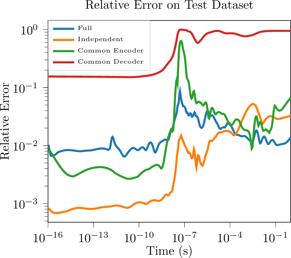
6 shows the average point-wise relative error 37 (for a test data set), on the collisional-radiative charge state model in 3.2, achieved by each approach presented above. Each approach was tested with approximately the same number of trainable parameters and the same training data. Based on the numerical result in 6, the "independent learning" approach shows the best performance, for the given problem, illustrated by i) the error being the lowest on average for the full time series and ii) its error spike near \(t=10^{-8}s\), the region where the dynamics evolve quickly, being lowest. The "common decoder" approach struggled, never outperforming any other method for any period of time. The "common encoder" and "full" approaches, on the other hand, had competitive performance with one another. Though they were not more accurate than "independent learning," except near \(t=10^{-3}s\), where steady state is usually reached. However, the rapid increase of error at \(t=10^{-8}s\) for the "common encoder" approach was uniquely large, leading to a two order of magnitude increase in error. For all the ODE numerical results (sections 3.1, 3.2), we only present results for the "independent learning" approach, while for the PDE problems (sections 3.3, 3.4), we present results only for the "full" approach. Note that for PDE problems such as 28 , a fine spatial discretization leads to a high-dimensional state space. As a result, the "independent learning" approach incurs a heavy computational cost during training, since using a separate network for each dimension results in a very large number of parameters (weights and biases). Hence, the results for the "independent learning" approach are not presented for PDE problems.




3 Numerical Experiments↩︎
In this section, we numerically demonstrate the effectiveness of LiLaN on a variety of prototype problems such as:
Robertson Stiff Chemical Kinetics Model [1]
Plasma Collisional-Radiative Model [2]
Allen-Cahn Phase Separation PDE [3]
Cahn-Hilliard Phase Separation PDE [3]
General experimental settings for all the problems and descriptions of methods adopted for comparison are detailed in [hyper95parameter].
3.1 Robertson Stiff Chemical Kinetics Model↩︎
The Robertson chemical kinetics problem is a prototype stiff system of ODEs that describes the concentration of three species of reactants in a chemical reaction [1]. The model has been widely used to evaluate the performance of stiff integrators in traditional numerical analysis. The reaction is characterized by the following system of ODEs: \[\begin{align} & \frac{d x_1}{d t} = -p_1 x_1 + p_3 x_2 x_3, \\ & \frac{dx_2}{dt} = p_1 x_1 - p_3 x_2 x_3 - p_2 x_2^2, \\ &\frac{dx_3}{dt} = p_2 x_2^2, \end{align} \label{rob}\tag{23}\] where the second species, \(x_2\), is the fastest evolving component and leads to numerical stiffness and difficulties in integration by explicit numerical solvers. In 23 , the three reaction rates are typically chosen as \(p_1 = 4 \cdot 10^{-2}\), \(p_2 = 3 \cdot 10^7\), and \(p_3 = 10^4\). Note that in 1 , we have the parameters of the StODE as \(\mathbf{p}=[p_1,\;p_2,\;p_3]\) and states as \(\boldsymbol{x}=[x_1,\;x_2,\;x_3]\).
3.1.1 Data Generation↩︎
For a given initial condition, \(\boldsymbol{x}_0\), and parameters, \(\mathbf{p}\), we integrate the system 23 with the Kvaerno5 stiff solver [38], from the Diffrax library [39], on a 50-point (i.e. \(M=50\) in 4 ) logarithmically scaled time grid, spanning from \(t=10^{-5}s\) to \(t=10^{5}s\). In this problem, the initial condition is fixed as \(\boldsymbol{x}_0= [1, 0, 0]\) and the reaction rates \(\mathbf{p}\) vary across training
samples. Similar to the data generation approach in [1], training
input samples \(\left( p_1,\;p_2,\;p_3 \right)\) were sampled from \([0.2\cdot10^{-2}, 0.6\cdot10^{-2}]\times [1.5 \cdot 10^{7}, 3.5 \cdot 10^{7}] \times [5 \cdot 10^{3},\;1.5 \cdot
10^{4}]\). The parameters of the training set, \(\left( p_1,\;p_2,\;p_3 \right)\), were sampled on a uniformly discretized grid of 16 linearly spaced collocation points in each domain. Thus, we consider a total of
\(4096\) training samples. An additional \(512\) validation samples and \(1000\) test samples were generated using a uniformly discretized grid of 8 and 10
points in each domain respectively.
3.1.2 Results↩︎
LiLaN was tested and compared with the NODE [21], DeepONet [24], and the Sulzer and Buck I and II approaches. The choice of latent dimension \(m\) for each method is provided in 8, 6.6. 7 shows a comparison of the average point-wise relative error, calculated via 37 , for each method when applied to the test dataset. From
7, we see that LiLaN outperformed DeepONet by approximately one order of magnitude over the entire time, and also outperformed NODE by several orders of magnitude. Compared to Sulzer and Buck I and II, the
performance of LiLaN is similar until the middle of the figure, where LiLaN takes the lead in accuracy. Note that the error of Sulzer and Buck I, the direct implementation of the methodology in [9], becomes greater than that of the modified Sulzer and Buck II with latent dimension expansion,
which reveals the benefit of increasing the problem dimensionality. The computation is done using single-precision floats, which means the error is close to machine precision for prediction on the early steps of the time series. The average error achieved
by different machine learning methods has been tabulated in 1 and shows that LiLaN achieved the lowest error out of all the approaches, when evaluated on the test dataset. 1
also shows that the method by Sulzer and Buck [9] produced a competitive
relative error compared to LiLaN. LiLaN outperformed NODE by two orders of magnitude and DeepONet by an order of magnitude. 8 depicts a simulated trajectory using LiLaN for a randomly chosen
set of parameters, \(\mathbf{p}\), from the test dataset, where we observe the predicted solution matches closely to the one calculated by the numerical solver. In 2, results on the
speedup achieved over the chosen traditional numerical solver (Kvaerno5 stiff solver) have been tabulated, where it is presented that the LiLaN approach achieved over 800x speedup in the task of simulating trajectories from 1000
initial conditions.
![Figure 7: Average point-wise relative error over time 37 when evaluating Robertson chemical kinetics model on test data. All methods, besides NODE, performed well on this problem, with LiLaN having a slight performance edge due to greater accuracy at the end of the time series t\in[10^0s,10^5s].](/article/2501.08423/_pdflatex/jlotdabw.png "fig:")
3.2 Plasma Collisional-Radiative Model↩︎
In this section, we consider a collisional-radiative (CR) model, for a lithium plasma, which has more significant multiscale behavior in comparison to the Robertson problem, in addition to being stiff. The CR model is a nonlinear dynamical system written as follows: \[\frac{d\mathbf{n}}{dt} = {\mathbf{R}}(\mathbf{n}) \cdot \mathbf{n}, \quad \mathbf{n}(0)=\mathbf{n}_{initial}. \label{eq:1}\tag{24}\] In 24 , \(\mathbf{n}\in\mathbb{R}^{n_x}\) and \({\mathbf{R}}\) is the \(n_x\times n_x\) rate matrix with nonlinear dependence on \(\mathbf{n}\). The rate matrix \({\mathbf{R}}\) contains a set of rules for the up-transitions and down-transitions of electrons between the \(n_x\) discrete excited state levels of the state vector \(\mathbf{n}\). The rate matrix explicitly depends on the temperature \(T_e\) and the electron density \(n_e\). The dependence on temperature comes from the fact that the electron distribution is assumed to be a Maxwellian distribution, parameterized by \(T_e\) [40]. The electron density is defined as \[n_e = \sum_{j=0}^{Z}jn_{j}, \label{electron95density}\tag{25}\] where \(Z\) denotes the atomic number of the plasma element (in our simulation we consider lithium, for which \(Z=3\)), \(j\) is the ion charge state, and \(n_j\) is the lithium ion density at charge state \(j\) given by 26. We have \(L=31\) in 26 , implying that \(\mathbf{n}\in \mathbb{R}^{94}\), i.e. there are \(94\) discrete excited states, and \[n_0 = \sum_{i=0}^{L-1}\mathbf{n}_{i}, \;\;\;\;n_1 = \sum_{i=L}^{2L-1}\mathbf{n}_{i}, \;\;\;\;n_2 = \sum_{i=2L}^{3L-1}\mathbf{n}_{i}, \;\;\;\;n_3 = \mathbf{n}_{3L}. \label{eq:4states}\tag{26}\] The traditional approach to solving 24 are methods well suited for stiff problems, such as Backward Differentiation Formula (BDF) methods, described in detail in [41]. These approaches are implicit linear multistep methods and require solving a system of \(n_x\) equations at each time step. Solving this system becomes very expensive when \(n_x\) is large, as is the case for CR models with high-Z element impurities or when \(L\) is large.
3.2.1 Data Generation↩︎
For data generation, 24 is integrated using the six-step BDF formula on a 400-step (i.e. \(M=400\) in 4 ) logarithmic time grid on \(t \in [1^{-16},1^0]\). We generate different initial conditions \({\mathbf{n}}_{initial}\) for 24 through two parameters \(n_A\) and \(n_{per}\) as follows: \[\begin{align} & \left( \mathbf{n}_{initial} \right)_0 = \left( 1 - n_{per} - 92 \cdot 10^{-5} \cdot n_{per} \right) \cdot n_A,\\ & \left( \mathbf{n}_{initial} \right)_1, \left( \mathbf{n}_{initial} \right)_2, \dots \left( \mathbf{n}_{initial} \right)_{92} = 10^{-5} \cdot n_{per} \cdot n_A,\\ & \left( \mathbf{n}_{initial} \right)_{93} = n_{per} \cdot n_A, \end{align} \label{f95map}\tag{27}\] where \(\left( \mathbf{n}_{initial} \right)_i\) denotes the \(i^{th}\) component of \(\mathbf{n}_{initial}\). We sample parameters \(\left( n_A,\;n_{per},\;T_e \right)\) from \([10^{14}, 10^{15}]\times [1 \cdot 10^{-3}, 2 \cdot 10^{-3}] \times [5,\;95]\), by considering a uniformly discretized grid (\(25\) equally spaced collocation points) in each variable, to generate the training data. This leads to a total of \(15625\) training samples. Here, \(n_A\) is the total number of lithium ions, of all charge states, in the plasma, \(T_e\) is the temperature in KeV, and \(n_{per}\) is a constant used to parameterize the initial electron distribution. An additional \(1000\) validation samples and \(4096\) test samples were also generated using respective grids of \(10\) and \(16\) linearly discretized collocation points. Note that the sum of the entries in \(\mathbf{n}_{initial}\) will be \(n_A\). In fact, the total number of electrons is conserved for all time steps of the simulation. Note that in 1 , we have the parameters \(\mathbf{p}=[T_e, \;n_A]\) and \(\boldsymbol{x}_0=\left( \mathbf{n}_{initial} \right)=\mathcal{F}\left( \mathbf{n_p} \right)\), where \(\mathbf{n_p}=[n_A, \;n_{per}]\) and \(\mathcal{F}\) is a map determined by 27 . In implementation, our approach only acts on the variables \(n_A\), \(T_e\), \(n_{per}\), and \(t\), and learning the parameterization 27 becomes part of the learning task.
3.2.2 Results↩︎
We demonstrate our approach on two cases:
CR charge state model: The aim here is to predict only the four charge states \(n_0,\dots, n_3\) in 26 .
Full CR model: The aim here is to predict the full state \(\mathbf{n}\in \mathbb{R}^{94}\) in 24 .
Results on the CR charge state model
LiLaN was tested and compared against NODE [21], DeepONet [24], the approach by Sulzer and Buck [9], as well as the modified Sulzer and Buck II. The choice of latent dimension \(m\) for each method is provided in 8, 6.6. The right subfigure of 9 shows a comparison of the average point-wise relative error, calculated via 37 , for each method when applied
to the test dataset. For this problem, we see that the error produced by LiLaN is lower than that of DeepONet. In particular, DeepONet has a large spike in error up to \(\mathcal{O}(10^{-1})\) near \(t=10^{-8}s\), which is typically the beginning of the temporal region where rapid changes in the solution take place. The error increase is present in the error of LiLaN, but it is not as significant, with the
error remaining on \(\mathcal{O}(10^{-2})\). The error of DeepONet decreases to nearly the same value as that of LiLaN in the temporal region where the steady state is typically reached, \(t\in[10^{-3}s, 10^{0}s]\). Additionally, NODE performs very poorly for this problem. Sulzer and Buck I and II produce a very close relative error to that of LiLaN throughout the simulation time, appearing
marginally less accurate in the initial range \(t \in [10^{-16}s, 10^{-10}s]\). The left subfigure of 9 depicts a simulated trajectory using LiLaN for a randomly chosen initial
condition and set of parameters, \(\mathbf{x}_0, \,\mathbf{p}\), from the test dataset. We observe that the predicted solution closely matches the numerical solution. 1 shows that Sulzer
and Buck II method produced slightly better relative error than LiLaN, when averaged over all time steps for all test samples. Sulzer and Buck I performed second best, followed very closely by LiLaN. The difference in their
averaged test errors was approximately \(1.1 \cdot 10^{-5}\). 1 also shows that DeepONet was an order of magnitude worse in terms of error than LiLaN and Sulzer and Buck I and
II, while NODE was notably inaccurate, lagging three orders of magnitude behind. The speedup achieved over the chosen numerical solver (BDF6 method) of LiLaN was almost 1500x, when generating full trajectories from 1000 test initial
conditions, as appears in 2.

Expanding Latent Space and Hidden Dimension

10 shows the change in training and test loss when different architectures are chosen, i.e. the dimension of the latent space and hidden layers were altered. For networks where the latent dimension was expanded (referred
to as "latent dimension expansion" in 10), all hidden layers were held at 100 neurons, while the latent dimension was allowed to vary. The x-axis of 10, for the "latent dimension expansion"
case, represents the ratio of the latent space dimension to the original problem dimension, i.e. \(\frac{m}{n_x}\) in 2.1. For networks where the hidden layer width was expanded (referred to as
"hidden dimension expansion" in 10), the latent dimension multiplier was kept at one, indicating that the latent space has the same dimension as the original system. The x-axis of 10, for
the "hidden dimension expansion" case, represents the number of neurons in each hidden layer. The result shows that much greater gains in accuracy are achieved by expanding the problem dimension to a higher-dimensional latent space. This agrees with our
motivation during the development of LiLaN, namely, that lifting a stiff problem to higher-dimensional latent space makes the problem easier to solve with high accuracy. In contrast, expanding the dimension of hidden layers, while not allowing
for latent expansion, resulted in very little gain in accuracy.
Results on the full CR model
To reduce the memory requirements associated with training the full CR model, we use \(4096\) data samples for training while \(2500\) samples are reserved for testing. The choice of
latent dimension \(m\) for each method is provided in 8, 6.6. For this higher-dimensional problem, training a NODE was not computationally feasible on our hardware
(NVIDIA Quadro RTX 5000) due to high memory requirements, even with the reduced training data set size. Hence, results for the NODE approach are not presented here. 11 (right) shows a comparison of the average
point-wise relative error, calculated via 37 , for each method, when applied to the test dataset. We see that LiLaN outperformed all other methods. Another key observation from 11
(right) is that, while all of the methods have a spike in error near \(t=10^{-8}s\), LiLaN’s error increase is the smallest by a wide margin, remaining on \(\mathcal{O}(10^{-2})\), while Sulzer and Buck I reaches \(\mathcal{O}(10^{-1})\) and DeepONet and Sulzer and Buck II increase to \(\mathcal{O}(10^{0})\). Recall
from 3.2.2, that \(t=10^{-8}s\) marks the approximate beginning of the region of the most rapid evolution of the dynamics, indicating that LiLaN handles this complex
behavior, which is a significant challenge to predict, the best of all methods considered. Moving to the left subfigure of 11, there is a depiction of the solution to the CR model using LiLaN for a
randomly chosen initial condition, \(\mathbf{x}_0\), and set of parameters, \(\mathbf{p}\), from the test dataset. The figure shows that LiLaN produces a good approximation of
the numerical solution. This approximation is particularly impressive near \(t=10^{-7}s\), where several components of the solution collapse in a nearly discontinuous manner. Again, the average error achieved by different
machine learning methods has been tabulated in 1, and additional results on the speedup achieved over the chosen traditional numerical solver (BDF6 method) have been tabulated in 2. We
observe from 1 that LiLaN produced the lowest relative error in comparison to all other methods. LiLaN outperformed DeepONet and Sulzer and Buck I by one order of magnitude. Sulzer and Buck II did
not perform well on this problem and had two orders of magnitude greater error than LiLaN. 2 reports the speedup achieved over the numerical solver (BDF6 method) by LiLaN, which was
approximately 800x in the same experiment as described in [sec:Robertson] [sec:chargestate] (CR charge state model).

3.3 Allen-Cahn PDE in 1D↩︎
The governing equation for the Allen-Cahn problem [3] is given below: \[u_t = \varepsilon u_{xx} + u - u^3, \label{sys95al}\tag{28}\] where the solution is \(u(x,t).\) The equation describes phase separation in iron alloys and has a second order diffusive term and a cubic reaction term [3]. In order to write 28 in the form 1 , the spatial domain is discretized and integrated as a system of ODEs by the method of lines [42]. The spatial domain, \(x \in [0,2\pi]\) is discretized by 201 linearly spaced points leading to dimension \(n_x=201\) in 1 . In the below discussions, \(\boldsymbol{x}\) denotes the vector containing the ordered set of discrete points on the spatial domain.
3.3.1 Data Generation↩︎
Initial conditions are generated using a sum of three sinusoidal waves as follows: \[\label{eq:ac95initialconditions} \mathbf{u}_0 = \sum_{i=1}^3 \alpha sin(\beta \boldsymbol{x}+ \phi) + \alpha cos(\beta \boldsymbol{x}+ \phi)\tag{29}\] \[\label{eq:ac95dists} \alpha \sim \mathcal{U}(0,1/6), \, \, \beta \sim \mathcal{U}_{discrete}(1,3), \, \, \phi \sim \mathcal{U}(0,2\pi),\tag{30}\] where \(\mathcal{U}\) represents the continuous uniform distribution and \(\mathcal{U}_{discrete}\) denotes the discrete uniform distribution. The amplitude \(\alpha\) and phase \(\phi\) are sampled from continuous uniform distributions, while the frequency \(\beta\) of each wave is sampled from a discrete uniform distribution where the frequencies \(1\), \(2\), or \(3\) are the discrete choices, each with equal probability of being selected. The integer frequencies ensure that the solution, \(\mathbf{u}\), is periodic on the problem domain. After the construction of the initial conditions, each is evolved in time using the ETDRK4 explicit, exponential integrator proposed in [43]. The problem is solved over the time interval \(t\in[0,10]\) seconds, which is discretized by \(101\) linearly spaced points, (i.e. \(M=101\) in 4 ). The dataset contains \(900\) samples for training, \(100\) samples for validation, and an additional \(200\) test samples, where each sample is a complete, time-integrated trajectory from a random initial condition generated by 29 .
3.3.2 Results↩︎
The results for this problem are presented in 12, where the left subfigure shows the numerical solution, while the middle subfigure shows the solution produced by LiLaN, from the same random initial condition,
unseen during training. We observe that the solutions are visibly identical. The right subfigure in 12 shows the absolute point-wise error between LiLaN and the numerical code. The errors are quite low nearly
everywhere, except at phase boundaries where the solution quickly switches between \(1\) and \(-1\), indicated by a quick shift from red to blue in the two leftmost subfigures of 12. This is a naturally challenging region to approximate, considering the sharp boundaries, yet the absolute pointwise error remains on \(\mathcal{O}(10^{-2})\). In terms of performance over the
entire test set, 13 presents the average error over time 37 , for five machine learning approaches: LiLaN, Sulzer and Buck I and II, DeepONet, and NODE. Each approach is trained with the
same data, hyperparameter settings, and approximately the same total number of trainable parameters. Additionally, the choice of latent dimension \(m\) for each method is provided in 8, 6.6. In 13, NODE performs slightly better than LiLaNduring the initial, short time interval. This is because NODE begins integration from a known initial condition, \(\boldsymbol{x}_0\) [21]. With no error accumulation at the starting point, the solution computed by NODE is most accurate in
the vicinity of \(\boldsymbol{x}_0\). 13 also shows that while LiLaNis particularly effective (with very low relative error) between 0s-7s, the approach by Sulzer and Buck [9] produced slightly lower error than LiLaNbetween 7s-10s. We also
observe that the relative errors of all methods converge to similar values toward the end of the simulation, suggesting a need for further investigation. However, the reason could be that all of the methods are nearly equally good for predicting the steady
state of the problem, a phenomenon that was observed between LiLaN, DeepONet, and Sulzer and Buck I and II in previous results [sec:Robertson] [sec:chargestate] (7 9). The average error achieved by different machine learning methods, for the
Allen-Cahn PDE, are included in 1, and report that the error produced by LiLaN is lowest in comparison to Sulzer and Buck I and II, DeepONet, and NODE, though they are all on the same order of magnitude.
LiLaN achieved 14.3x speedup over the solver (ETDRK4 method), as shown in 2. The experiment to test the speed of LiLaN versus the traditional solver is the same as in 3.1. The speedup is less radical than previous results sections because exponential integrators are already extremely efficient for simulating stiff PDEs, meaning any speedup is a significant success.

3.4 Cahn-Hilliard PDE in 1D↩︎
The governing equation for the Cahn-Hilliard problem [3] is given below: \[u_t = \alpha \left( -u_{xx} - \gamma u_{xxxx} + (u^3)_{xx} \right)\] where the solution is \(u(x,t).\) This is another equation describing phase separation in alloys, but with much more complex physics due to the presence of the higher-order derivatives in the governing equation. Just as with the Allen-Cahn problem (3.3), the spatial domain is discretized and integrated as a system of ODEs by the method of lines [42]. The spatial domain, \(x \in [-1,1]\) is discretized by 201 linearly spaced points, and is denoted by \(\boldsymbol{x}\) in the below discussions.
3.4.1 Data Generation↩︎
Initial conditions in the Cahn-Hilliard problem are generated as follows: \[\label{eq:ch95initialconditions} \mathbf{u}_0 = \alpha sin(\beta \pi (\boldsymbol{x}+1) + \phi) + \alpha cos(\beta \pi (\boldsymbol{x}+1) + \phi),\tag{31}\] \[\label{eq:ch95dists} \alpha \sim \mathcal{U}(0.1,0.6), \, \, \beta \sim \mathcal{U}_{discrete}(1,3), \, \, \phi \sim \mathcal{U}(0,2\pi),\tag{32}\] where \(\mathcal{U}\) represents the continuous uniform distribution and \(\mathcal{U}_{discrete}\) denotes the discrete uniform distribution. For each initial condition, generated by 31 , the amplitude \(\alpha\) and phase \(\phi\) are sampled from continuous uniform distributions, specified in 32 , while the frequency coefficient \(\beta\) of the wave is sampled from a discrete uniform distribution where the frequencies \(1\), \(2\), or \(3\) are the discrete choices, each with equal probability of being selected. The integer frequencies ensure that the solution, \(\mathbf{u}\), is periodic on the problem domain. After the construction of the initial conditions, each is evolved in time using the ETDRK4 explicit, exponential integrator [43]. The problem is solved over the time interval \(t\in[0,20]\) seconds, which is discretized by \(401\) linearly spaced points (i.e. M = 401 in 4 ). The dataset contains \(900\) samples for training, \(100\) samples for validation, and an additional \(200\) test samples, where each sample is a complete, time-integrated trajectory from a random initial condition generated by 31 .
3.4.2 Results↩︎
14 (left) shows a solution generated by numerical code, while 14 (middle) shows the solution produced by LiLaN, from the same initial condition that was not seen during training. The
solutions are strikingly similar visibly. 14 (right) shows the absolute point-wise error between our approach and the numerical code for the example initial condition considered. Notice that on this problem, the largest errors
are not at steady state phase boundaries, in contrast to the Allen-Cahn PDE results from 3.3. Instead, high errors are most prevalent in the initial transient evolution before the solution reaches steady state, while the
steady state has lower error than in 3.3. In terms of performance over the entire test set, 15 depicts the average error over time 37 , for LiLaN, Sulzer and
Buck I and II, DeepONet, and NODE. Each approach is trained with the same data, hyperparameter settings, and approximately the same total number of trainable parameters. Again, the choice of latent dimension \(m\) for each
method is provided in 8, 6.6. From 15 we see that LiLaN outperformed both NODE and DeepONet for prediction on the Cahn-Hilliard PDE. NODE performs slightly
better than LiLaN during the initial, short time interval. The reason for this has been highlighted in 3.3.2. We also observe that the approach of Sulzer and Buck I and II produce a very close relative error
to that of LiLaN towards the end of the simulation time. This, again, could be due to the fact that predicting the steady state is easier that predicting the time dependent evolution. Looking at the example in 14,
the evolution is done before \(t=3s\), which is typical across the entire dataset, with some exceptions where the evolution is slower. Now, the region of 15 prior to \(t=4s\) is where LiLaN performs the best, beating all other methods, suggesting that it is uniquely suited for handling the time dependent portion of the solution. 1 illustrates
that the average relative error produced by LiLaN is lowest of all methods tested. Significantly, DeepONet has an order of magnitude greater error than LiLaN, while the Sulzer and Buck I and II and NODE methods, though less
accurate than LiLaN, achieve errors on the same order of magnitude. The speedup achieved over the chosen traditional numerical solver (ETDRK4 method) is tabulated in 2, showing that LiLaN was
13.7x faster when generating full trajectories from 1000 test initial conditions. Again, even though the speedup is less than that of the ODE problems, it is still impressive due to the competition being conducted against an exponential integrator.

3.5 Improving Training Efficiency of LiLaN↩︎
Thus far, all previous sections have presented results for LiLaN training in the data-rich regime. In each problem considered, data is relatively cheap, but this may not hold true for other engineering tasks which require surrogate
modeling. Therefore, it provides valuable insight to investigate the accuracy of the LiLaN model in the data-poor regime. On the other hand, a data-intensive training procedure can pose a heavy computational burden for training any model. This
is especially the case when using large networks for high-dimensional problems (for example, the PDE problems in [sec:AC] [sec:CH]). In situations where the available memory or training time budget have strict limitations, data reduction is an effective tool to meet project requirements. This being the case, the accuracy of
LiLaN surrogates under different data reduction schemes must be examined. In this section, we consider two data reduction procedures and their ramifications for LiLaN :
The first strategy involves reducing the training data and investigating the effect on the generalization performance of
LiLaN. In particular, we study how reducing the number of sample trajectories (i.e. the parameter \(N\) in 4 ) affects the performance ofLiLaN. Note that smaller training datasets significantly improve the computational efficiency during training while also reducing the data generation time. Additionally, in some applications, data cannot be generated at will and is limited to data from real-world sensor observations. For these reasons, it is highly desirable that theLiLaNarchitecture is robust and can achieve a high degree of generalization accuracy with varying amounts of data.The second strategy involves the use of coarsened time discretizations in training, meaning reduction of the parameter \(M\) in 4 ) and investigating the impact on the generalization performance of
LiLaN. Reducing the discretization of training data means potentially massive savings on memory during training. This, in turn, means that one can use a greater number of samples for a fixed training memory budget or can simply reap the rewards of lower memory cost and faster training speed.
3.5.1 Reducing Training Sample Size \(N\) in 4↩︎
The first strategy for improving the training efficiency of LiLaN considers reducing the number of sample trajectories (i.e. the parameter \(N\) in 4 ). For the Robertson (3.1) and full CR models ([sec:full-CR]), the original network was trained with \(4096\) samples from a
three-dimensional parameter space. To understand how the prediction accuracy degrades with training data size, several smaller datasets were created by repeatedly reducing the number of training samples by a factor of two. For the CR charge state model (3.2.2), the initial training utilized \(15625\) samples from a three-dimensional parameter input space. For this problem, smaller datasets were created by repeatedly reducing the number
of training samples, this time by a factor of five. The smallest dataset, for each ODE problem considered, contained only the eight corners of the original 3-dimensional parameter space.
From 16 (left subfigure) we see that for the Robertson model (3.1), using only \(128\) samples, a LiLaN can be trained to achieve error on the
same order of magnitude as a network of the same architecture trained with \(4096\) samples (a reduction of \(32\)x). For the CR charge state model (16, (middle
subfigure)), \(125\) samples were required to train a network which achieved error on the same order of magnitude of the original network trained with \(15625\) samples. Finally, after \(256\) training samples, the LiLaN’s final accuracy on the full CR test dataset does not significantly improve if more samples are provided, as seen in 16 (right subfigure). From these ODE
problem results, we observe that the amount of data used for training LiLaN surrogates can be reduced significantly while maintaining accuracy, indicating that data reduction via reducing the training samples is a viable data reduction
strategy.
For completeness, the same sample reduction experiment was performed on each of the two PDE problems ([sec:AC] [sec:CH]). In each case, the original dataset of \(900\) samples was repeatedly reduced by \(100\) samples and used to train a new model. The smallest dataset contained \(100\) total sample trajectories. The change in accuracy with respect to sample size is shown in 17. 17 shows that for each of the PDE problems, adding more samples typically resulted in a significant decrease in the relative error, though this decrease does slow after the first few hundred samples are added in both cases. However, this does suggest that reducing the training data may not be a favorable option for improving the computational efficiency, as these problems might require a large number of samples to guarantee a low relative error.

3.5.2 Using Coarse Time Discretizations in Training↩︎
An additional strategy to reduce the data and memory requirements of training the network is to consider a coarse time grid for the sample trajectories. In this section, we investigate the effect of reducing the parameter \(M\) in 4 on the performance of LiLaN. We consider different time discretizations by removing large numbers of time steps from the training and validation data and using this new
dataset to train the networks. Examples of different time grids considered for training neural networks are shown in 18 19 20 21 22 (left subfigures). For assessing the performance, we retain the original test data, which still has a fine discretization in time. The main purpose of this study is to investigate whether coarsening the discretization in time is
an effective means to reduce data, while maintaining the test accuracy of LiLaN.
Our results indicate that, in all test problems, data reduction by coarsening the underlying time discretization of data trajectories proves to be an effective path to reducing computational cost while maintaining test accuracy. The results of our
experiments are shown in 18 19 20 21 22. The left subfigure in each of the aforementioned figures depicts
the new time discretizations used in training, while the right subfigure shows the change in relative error compared to how many steps were skipped. The x-axis of the right subfigures, labeled "Skipped Steps," indicates the number of time steps which were
removed between steps in the original discretization. For example, if skipped steps \(= 10\), then we retain the time steps \(\{x_i\}_{i=0,\, 10,\, 20,\, \cdots,\, M-10,\, M}\) for each
training and validation sample. It is important to note that the accuracy reported is still evaluated on the test dataset, which is not downsampled in time. In each of 18 19 20 21 22, the results indicate that a significant number of time steps can be removed from the training discretization before accuracy degrades significantly. Specifically, 18, shows that on the Robertson ODE problem (3.1), we may take skipped steps = 8 before seeing the first major drop in accuracy. For the CR charge states and full CR models (3.2), 19 20 show that generalization error does not decrease until 20 steps are skipped between each preserved step. In the case of the Allen-Cahn PDE (3.3), 21 suggests that accuracy deteriorates very slowly in relation to the number of skipped steps, again with a falling off observed after gaps of 20 are removed from the data. For the final problem
considered, in 22 we see that skipping a remarkable 40 steps results in almost no loss of test performance, and finally after 80 steps there is a larger decline in accuracy for the Cahn-Hilliard PDE (3.4). These results lead us to believe that coarsening the time discretization of the data is a very effective data reduction technique for LiLaN surrogates. However, the ability to train on coarse discretizations
naturally begs the question of why LiLaN is so effective after data is reduced in this manner. To attempt to answer this question we devised an additional experiment to determine whether the time transformation network, \(\boldsymbol{\tau}\), plays a significant role in LiLaN robustness to training on temporally downsampled discretizations of the original training data.
3.6 Importance of Learned Time Transformation↩︎
In this section, we investigate the importance of the nonlinear time transformation (\(\boldsymbol{\tau}\left( t,\;\boldsymbol{x}_0,\;\mathbf{p}; \;\boldsymbol{\nu} \right)\) in 3 ) on
all problems considered in this work. The following experiments were inspired by the results on temporally downsampling training data, presented in 16. Additionally, since one of the key differences between LiLaN and
the methodology of Sulzer and Buck [9] is the learned, nonlinear
transformation of the time variable, we thought it informative to test the results of the LiLaN architecture if the time transformation was removed. In particular, instead of 3 , we consider the solution in
the latent space to have the following form: \[\boldsymbol{y}\left( t,\;\boldsymbol{x}_0,\;\mathbf{p} \right)= \boldsymbol{{\boldsymbol{e}}}(\boldsymbol{x}_0,
\mathbf{p};\;\boldsymbol{\beta}) + t\;\boldsymbol{\boldsymbol{c}}(\boldsymbol{x}_0, \mathbf{p};\;\boldsymbol{\alpha}). \label{eq:no95time95transform}\tag{33}\] where time, \(t\), is first log scaled with the
base \(10\) logarithm and then rescaled to the range \([0, 1]\). This new transform of the time variable is the same as used in [9]. The right subfigure of 18 19
20 21 22 explore the benefit of the time transformation in the context of data reduction described in 3.5.2. The black circles
represent the error for LiLaNs trained with a learned time transformation, while the red dots indicate the error for LiLaNs trained with the simple, rescaled time variable. For the rest of this section, we will refer to the
LiLaNs trained without using a time transformation \(\boldsymbol{\tau}\) network as \(\texttt{LiLaN}_{\cancel{\boldsymbol{\tau}}}\). Observing the right subfigures of 19 21 22, we see a clear benefit in terms of final relative error achieved when using LiLaN over \(\texttt{LiLaN}_{\cancel{\boldsymbol{\tau}}}\). Specifically, there are two important features to recognize in each figure. First, in each case, the error is lower for LiLaN. Second, when coarsening the time
discretization of training data, the accuracy of \(\texttt{LiLaN}_{\cancel{\boldsymbol{\tau}}}\) degrades significantly more quickly. On the CR charge state model (19 right subfigure),
LiLaN with skipped steps \(=20\) outperformed \(\texttt{LiLaN}_{\cancel{\boldsymbol{\tau}}}\) with skipped steps \(=12\). For the Allen-Cahn PDE
(21 right subfigure) LiLaN with skipped steps \(=20\) achieved lower error than a \(\texttt{LiLaN}_{\cancel{\boldsymbol{\tau}}}\) with skipped steps
\(=10\). For the Cahn-Hilliard PDE (22 right subfigure) LiLaN with skipped steps \(=50\) outperformed a \(\texttt{LiLaN}_{\cancel{\boldsymbol{\tau}}}\) with skipped steps \(=25\). These results suggest that the learned time transformation helps the LiLaN architecture in modeling the
time dependence of the underlying dynamical system with fewer temporal data points. This result also reinforces the claims from [sec:full-CR] [sec:AC] [sec:CH] that LiLaN is very good at modeling time dependent behaviors. In situations where memory budget is
very limited or a large number of initial conditions must be trained over, LiLaN will be the better choice of architecture, in comparison to \(\texttt{LiLaN}_{\cancel{\boldsymbol{\tau}}}\), since each sample
trajectory will require fewer snapshots in time, which greatly reduces the memory impact in training for each sample trajectory.
For the Robertson ODE and full CR model, shown in the right subfigures of 18 20 respectively, we did not observe significant benefits of a learned time transformation. Therefore, we conclude
that the importance of the learned time transformation is problem dependent, however in the majority of cases investigated in our work, LiLaN allowed for greater data reduction than \(\texttt{LiLaN}_{\cancel{\boldsymbol{\tau}}}\). Considering the fact that the additional training cost associated with training the time transformation network \(\boldsymbol{\tau}\) is
negligible, the use of LiLaN (with time transformation \(\boldsymbol{\tau}\)) is generally advisable, instead of \(\texttt{LiLaN}_{\cancel{\boldsymbol{\tau}}}\).


4 Summary of results↩︎
1 shows the prediction error computed using 38 for each machine learning method, on each problem. We see that LiLaN produced the lowest relative error for all the problems except the
CR charge state problem, where the Sulzer and Buck II approach, a modified form of the method in [9], slightly outperformed LiLaN, though the errors were on the same order of magnitude. 1 also shows that for the Robertson ODE Model 3.1,
LiLaN outperformed NODE by approximately two order of magnitude and outperformed DeepONet and Sulzer and Buck I by one order of magnitude in terms of the relative error achieved. For the CR charge state model, LiLaN and Sulzer and
Buck I and II achieved errors on the same order of magnitude which were three and one orders of magnitude less than the errors of NODE and DeepONet respectively. For the full CR model, DeepONet and Sulzer and Buck I exceeded the error of
LiLaN by an order of magnitude. On the same problem, Sulzer and Buck II struggled significantly compared to LiLaN , having two orders of magnitude greater relative error. On the two PDE problems, all methods had the same order of
magnitude error, on the test dataset; however, LiLaN ’s was quantitatively the lowest. The one notable exception was DeepONet, which had one order of magnitude greater error on the Cahn-Hilliard problem compared to the other methods.
2 shows the speedup of LiLaN in comparison to the traditional stiff numerical solver used to generate the data in each problem. To measure the speedup achieved, \(1000\)
initial conditions were chosen to run the simulations for each problem. 2 shows the total time taken by both the numerical solver and LiLaN to compute the solutions for all the \(1000\) initial conditions. We see that LiLaN achieved \(\mathcal{O}(10^1)\)-\(\mathcal{O}(10^3)\) speedup on all problems, in terms of wall clock
computation time, with especially remarkable speedup displayed on the three ODE problems ([sec:Robertson] [sec:CR-model]).
| Relative Error | |||||
|---|---|---|---|---|---|
| Problem | Robertson | CR charge state | Full CR model | Allen-Cahn | Cahn-Hilliard |
| NODE | \(1.112\cdot10^{-2}\) | \(2.209\cdot10^{0}\) | \(\mathbf{OOM}\) | \(6.070\cdot10^{-2}\) | \(8.810\cdot10^{-2}\) |
| DeepONet | \(1.697\cdot10^{-3}\) | \(2.003\cdot10^{-2}\) | \(3.968\cdot10^{-2}\) | \(8.589\cdot10^{-2}\) | \(2.492\cdot10^{-1}\) |
| Sulzer and Buck I | \(1.475\cdot10^{-3}\) | \(1.970\cdot10^{-3}\) | \(2.132\cdot10^{-2}\) | \(3.633\cdot10^{-2}\) | \(5.627\cdot10^{-2}\) |
| Sulzer and Buck II | \(7.645\cdot10^{-4}\) | \(\mathbf{1.598\cdot10^{-3}}\) | \(1.797\cdot10^{-1}\) | \(3.391\cdot10^{-2}\) | \(5.517\cdot10^{-2}\) |
| \(\mathbf{2.80\cdot10^{-4}}\) | \(1.981\cdot10^{-3}\) | \(\mathbf{7.486\cdot10^{-3}}\) | \(\mathbf{1.072\cdot10^{-2}}\) | \(\mathbf{4.741\cdot10^{-2}}\) | |
| Speed tests in wall clock time | |||||
|---|---|---|---|---|---|
| Problem | Robertson | CR charge state | Full CR model | Allen-Cahn | Cahn-Hilliard |
| Numerical Solver | \(6232.8\)s | \(11034.1\)s | \(10955.5\)s | \(53.25\)s | \(212.1\)s |
| \(7.648\)s | \(7.366\)s | \(13.604\)s | \(3.729\)s | \(15.485\)s | |
| Speedup | \(\mathbf{815.0x}\) | \(\mathbf{1498.0x}\) | \(\mathbf{805.3x}\) | \(\mathbf{14.3x}\) | \(\mathbf{13.7x}\) |
5 Conclusion↩︎
In this paper, we have presented a novel, machine learning approach, called LiLaN, for fast and accurate simulation of stiff, nonlinear, ordinary and partial differential equations. LiLaN is inspired by kernel methods in which
the original problem under consideration is featurized/lifted to (much) higher dimensional feature spaces where the problem is now easier. In particular, LiLaN, via nonlinear neural networks, lifts the original stiff problems into higher
dimensions where the problem is no longer stiff. Unlike kernel methods which rely on particular feature maps to organize the latent dynamics so that hopefully it is easier to simulate, LiLaN forces the latent dynamics to be trivially linear,
and then learns the nonlinear feature maps using neural networksthe encoders. With linear latent dynamics that admits analytical solutions, no numerical integration, but instead evaluations of encoders/decoders, are needed during the inference stage, and
this is key to LiLaN’s real-time efficiency. LiLaN is thus a solution operator approach that learns the flow maps of nonlinear systems of ODEs. Indeed, theoretical results show that LiLaN can approximate an arbitrary
continuous flow map to any desired accuracy and that the latent dimension is independent of the accuracy. Various numerical results with varying dimensionality, complexity, and stiffness have been presented to demonstrate the speed and accuracy of
LiLaN against contemporary machine learning and numerical methods. Numerical results also show that the temporal nonlinear mapping into the latent space plays a vital role in achieving better generalization performance especially when using
coarse time grids for training the networks. In particular, LiLaN architectures show better generalization capabilities compared to a direct learning method for approximating the flow map of a system of ODEs. It should be pointed out that, in
this paper, though the motivation and numerical examples for LiLaN are stiff ODEs, it is equally applicable to non-stiff ODEs. Part of our future work will focus on additional theoretical analysis (non-asymptotic analysis) and numerical
results to address the question of why LiLaN outperformed the direct learning approach for learning flow maps. For many problems, data generation may be costly, and part of our future work is to develop algorithms for adaptive data sampling
(active learning) to reduce the amount of data required to train each model, while also answering the question of finding the optimal neural network architecture (number of layers, number of neurons in each layer) for prediction such as in [44].
6 Acknowledgments↩︎
This research is partially funded by the National Science Foundation award NSF-OAC-2212442 and by the Department of Energy awards DE-SC0024724 and DE-SC0024633. The authors would like to thank Wesley Lao and Hai Nguyen for productive conversations. The authors also acknowledge the Texas Advanced Computing Center (TACC) at The University of Texas at Austin for providing HPC resources that have been vital to the research results reported within this paper. URL: http://www.tacc.utexas.edu
General setting for numerical experiments
6.1 Data Transformations↩︎
ODE Problems: [sec:Robertson] [sec:CR-model]
To address the multiscale nature of the data in the three ODE problems, as a preprocessing step, all time series data is log scaled using the base \(10\) logarithm. This procedure reduces the scale separation of different
components of the solution. As an additional training aid, all network inputs, apart from time, are scaled independently to the range \([-1,1]\). Finally, the time discretization points are log scaled, using the base 10
logarithm, and then rescaled to fit the range \([0,1]\) seconds. Additionally, since each of the ODE problems is conservative (Robertson ODE has conservation of total concentration and CR ODEs have conservation of total
number of electrons), we implement conservation constraints implicitly, by applying a softmax to the output of the decoder and multiplying by the appropriate constant (known from \(\boldsymbol{x}_0\)) to obtain a solution
satisfying the conservation constraint.
PDE Problems: [sec:AC] [sec:CH]
For both PDE models, the data all lies on the range \([-1,1]\), so no rescaling is required. However, the time discretization points are rescaled to fit the range \([0,1]\) seconds.
6.2 Training for Multiscale Stiff Systems↩︎
In all of the ODE ([sec:Robertson] [sec:CR-model]) test problems presented in this paper, the unique degrees of freedom in the solution vary by several orders of magnitude. This led to challenges in training with traditional loss functions such as mean squared error (MSE). In training, such loss functions were heavily biased toward learning the large magnitude components of the solution. To remedy this issue, we considered an absolute relative error loss function. The use of relative error balances out the magnitudes of errors for each individual degree of freedom. \[\label{eq:J95old95rel} \mathcal{L}(\mathbf{X}; \boldsymbol{\alpha}, \boldsymbol{\beta}, \boldsymbol{\nu}, \boldsymbol{\theta}) = \frac{1}{(N+1) \cdot (M+1)}\sum_{i=0}^{N}\sum_{j=0}^{M}\left|\frac{\mathbf{x}_{i}(t_{j}) - \mathbf{\hat{x}}_{i}(t_{j})}{\mathbf{x}_{i}(t_{j})}\right|.\tag{34}\] where, the predicted state \(\hat{\boldsymbol{x}}_{i}(t_j)\) for time \(t_j\) and for the \(i^{th}\) training input \(\{\left( \boldsymbol{x}_0 \right)_i, \mathbf{p}_i\}\) is given by 36 . \({\boldsymbol{x}}_{i}(t_j)\) denotes the actual state at time \(t_j\) for the \(i^{th}\) input. However, this loss function still has the problem that overshooting errors are punished much more harshly than undershooting errors. Finally, we settled on the following loss function which resolves the unbalanced penalties between overshooting and undershooting. \[\label{eq:J} \mathcal{L}(\mathbf{X}; \boldsymbol{\alpha}, \boldsymbol{\beta}, \boldsymbol{\nu}, \boldsymbol{\theta}) = \frac{1}{N+1}\sum_{i=0}^{N}\prod_{j=0}^{M}10^{\frac{1}{M+1}\left|\mathbf{x}_{i}(t_{j}) - \mathbf{\hat{x}}_{i}(t_{j})\right|},\tag{35}\] \[\mathbf{\hat{x}}_{i}(t_{j}) = \boldsymbol{d}\left( \boldsymbol{e}\left( \left( \mathbf{x}_0 \right)_{i},\mathbf{p}_{i}; \boldsymbol{\alpha} \right) + \boldsymbol{\tau}(t_j, \left( \mathbf{x}_0 \right)_{i},\mathbf{p}_{i}; \boldsymbol{\nu}) \;\circ \;\boldsymbol{c}(\mathbf{x}_{0_i},\mathbf{p}_{i}; \boldsymbol{\beta});\boldsymbol{\theta}\right). \label{for95prop}\tag{36}\] In 34 and 35 , \(\mathbf{X}\) is a third order tensor containing \(\left[ \mathbf{x}(t_{j}) \right]_{i}\) for all samples, \(s = 0, \ldots, N_s\), and all times, \(t = 0, \ldots, N_t\), in the dataset.
The above loss function is used for the ODE problems which are trained using a log scaled version of the original data. For the PDE problems ([sec:AC] [sec:CH]), the data is not log scaled so a different loss function was chosen. We do not use an absolute error style loss function, since some of the true data is 0, meaning the relative error will be undefined at those points. Instead, the evaluation metric 38 was used as the loss function in training.
6.3 Error Evaluation Metrics↩︎
The plots, in this paper, depicting point-wise relative error over time, report the relative error in the Euclidean norm, averaged over all \(N\) samples, given as \[\label{eq:R1} \mathcal{R}_1 = \frac{1}{N+1}\sum_{i=0}^{N}\frac{\left|\left|\mathbf{x}_{i}(t_{j}) - \mathbf{\hat{x}}_{i}(t_{j})\right|\right|_{2}}{\left|\left|\mathbf{x}_{i}(t_{j})\right|\right|_{2}}.\tag{37}\] 1 reports the point-wise relative error in the Euclidean norm, averaged over all \(N\) samples and \(M\) time steps, given as: \[\label{eq:R2} \mathcal{R}_2 = \frac{1}{(N+1) \cdot (M+1)}\sum_{i=0}^{N}\sum_{j=0}^{M}\frac{\left|\left|\mathbf{x}_{i}(t_{j}) - \mathbf{\hat{x}}_{i}(t_{j})\right|\right|_{2}}{\left|\left|\mathbf{x}_{i}(t_{j})\right|\right|_{2}}.\tag{38}\]
6.4 Description of methods adopted for comparison↩︎
LiLaN is compared with the four approaches described below: \[\begin{align}
\text{DeepONet}&: \text{An operator learning approach with branch networks, taking the state as its input, and trunk}\\
&\text{ \;\;networks, taking time as its input, with the inner product of their respective outputs being the}\\
&\text{ \;\;predicted solution, as described in \cite{goswami2023learningstiffchemicalkinetics}.}\\
\text{Neural ODE}&: \text{A scheme for approximating the right hand side of a parameterized ODE with a neural network}\\
&\text{\;\;\; and solving using traditional numerical integration schemes, as described in \cite{Lee_2021}. The solver used}\\
&\text{ \;\;with the Neural ODEs implemented in our work is an implicit Euler scheme. Data and time steps}\\
&\text{ \;\;are rescaled in ways resembling the methodology in \cite{Kim_2021}.}\\
\text{Sulzer and Buck I}&: \text{A Neural ODE approach in a reduced dimension (n_x \ge m) latent space, described in \cite{sulzer2023speedingastrochemicalreactionnetworks}, in which}\\
&\text{\;\;\;the right hand side is considered a constant function of the encoded initial condition.}\\
\text{Sulzer and Buck II}&: \text{A Neural ODE approach in an expanded dimension (n_x \le m) latent space, in which the right hand}\\
&\text{\;\;\;side is considered a constant function of the encoded initial condition. This is a modified version}\\
&\text{\;\;\;of the approach described in \cite{sulzer2023speedingastrochemicalreactionnetworks}.}\\
\end{align}\]
6.5 Architectural Details↩︎
[arc_det_1,arc_det_2,arc_det_3,arc_det_4,arc_det_5] show the neural network architectures
used for each machine learning method and problem setting. Each network uses the \(tanh\) activation function at each hidden layer and has a linear output layer. The notation, [*,...,*], indicates the number of neurons in
each layer for a multilayer perceptron network, including the initial input layer. Recall that, since we use the independent architectural variants for testing each ODE problem, there is one network of each type per degree of freedom in the system of ODEs
for LiLaN and DeepONet. Networks following the "independent" architectural variant from 2.3 are labeled with a \(*\) in the following table. All other networks are
implemented as the "full" variant from 2.3. The labels (DR1) and (DR2) denote the architectures which were used in the data reduction experiments, described in 3.5. The label (DR1)
indicates our approach, while (DR2) indicates the omission of the time transform. For problems, in the table without a (DR1) entry, the same architecture used in 3 was used for the data reduction experiments.
| Approach | |||||
|---|---|---|---|---|---|
| Problem | Encoder \(\bs{e}\) | Encoder \(\bs{c}\) | Encoder \(\boldsymbol{\tau}\) | Decoder \(\bs{d}\) | Total Parameters |
| Robertson\(^*\) | [\(3\),\(20\),\(5\)] | [\(3\),\(20\),\(5\)] | [\(4\),\(20\),\(5\)], \(5\) | [\(5\),\(20\),\(20\),\(1\)] | \(3,423\) |
| Robertson\(^*\) (DR2) | [\(3\),\(23\),\(5\)] | [\(3\),\(23\),\(5\)] | N/A | [\(5\),\(23\),\(23\),\(1\)] | \(3,414\) |
| CR Charge States\(^*\) | [\(3\),\(20\),\(5\)] | [\(3\),\(20\),\(5\)] | [\(4\),\(20\),\(5\)], \(5\) | [\(5\),\(20\),\(20\),\(1\)] | \(4,564\) |
| CR Charge States\(^*\) (DR2) | [\(3\),\(23\),\(5\)] | [\(3\),\(23\),\(5\)] | N/A | [\(5\),\(23\),\(23\),\(1\)] | \(4,552\) |
| Full CR\(^*\) | [\(3\),\(40\),\(20\)] | [\(3\),\(40\),\(20\)] | [\(4\),\(40\),\(20\)], \(20\) | [\(20\),\(40\),\(40\),\(1\)] | \(518,974\) |
| Full CR\(^*\) (DR1) | [\(3\),\(40\),\(5\)] | [\(3\),\(40\),\(5\)] | [\(4\),\(40\),\(5\)], \(5\) | [\(5\),\(40\),\(40\),\(1\)] | \(287,734\) |
| Full CR\(^*\) (DR2) | [\(3\),\(44\),\(5\)] | [\(3\),\(44\),\(5\)] | N/A | [\(5\),\(44\),\(44\),\(1\)] | \(290,554\) |
| Allen-Cahn | [\(201\),\(201\),\(201\)] | [\(201\),\(201\),\(201\)] | [\(202\),\(201\),\(201\)], 201 | [\(201\),\(201\),\(201\),\(201\)] | \(365,820\) |
| Allen-Cahn (DR1) | [\(201\),\(100\),\(20\)] | [\(201\),\(100\),\(20\)] | [\(202\),\(100\),\(20\)], 20 | [\(20\),\(100\),\(100\),\(201\)] | \(99,281\) |
| Allen-Cahn (DR2) | [\(201\),\(155\),\(20\)] | [\(201\),\(155\),\(20\)] | N/A | [\(202\),\(155\),\(155\),\(20\)] | \(99,596\) |
| Cahn-Hilliard | [\(201\),\(201\),\(201\)] | [\(201\),\(201\),\(201\)] | [\(202\),\(201\),\(201\)], 201 | [\(201\),\(201\),\(201\),\(201\)] | \(365,820\) |
| Cahn-Hilliard (DR1) | [\(201\),\(100\),\(20\)] | [\(201\),\(100\),\(20\)] | [\(20\),\(100\),\(201\)], 20 | [\(20\),\(100\),\(100\),\(201\)] | \(99,281\) |
| Cahn-Hilliard (DR2) | [\(201\),\(155\),\(20\)] | [\(201\),\(155\),\(20\)] | N/A | [\(20\),\(155\),\(155\),\(201\)] | \(99,596\) |
| Sulzer and Buck I | ||||
|---|---|---|---|---|
| Problem | Encoder | Neural ODE | Decoder | Total Parameters |
| Robertson | [3,49,3] | [3,49,3] | [3,49,49,3] | \(3,488\) |
| CR Charge States | [3,55,4] | [4,55,4] | [4,55,55,4] | \(4,522\) |
| Full CR | [3,645,16] | [16,645,16] | [16,645,645,94] | \(522,576\) |
| Allen-Cahn | [201,390,34] | [34,390,34] | [34,390,390,201] | \(363,749\) |
| Cahn-Hilliard | [201,390,34] | [34,390,34] | [34,390,390,201] | \(363,749\) |
| Sulzer and Buck II | ||||
|---|---|---|---|---|
| Problem | Encoder | Neural ODE | Decoder | Total Parameters |
| Robertson | [3,33,15] | [15,33,15] | [15,33,33,3] | \(3,432\) |
| CR Charge States | [3,36,20] | [20,36,20] | [20,36,36,4] | \(4,616\) |
| Full CR | [3,67,1880] | [1880,67,1880] | [1880,67,67,94] | \(518,950\) |
| Allen-Cahn | [201,250,201] | [201,250,201] | [201,250,250,201] | \(365,603\) |
| Cahn-Hilliard | [201,250,201] | [201,250,201] | [201,250,250,201] | \(365,603\) |
| DeepONet | |||
|---|---|---|---|
| Problem | Branch Network | Trunk Network | Total Parameters |
| Robertson | [\(3\),\(20\),\(20\),\(5\)] | [\(1\),\(20\),\(20\),\(5\)] | \(3,510\) |
| CR Charge States | [\(3\),\(20\),\(20\),\(5\)] | [\(1\),\(20\),\(20\),\(5\)] | \(4,680\) |
| Full CR | [\(3\),\(42\),\(42\),\(20\)] | [\(1\),\(42\),\(42\),\(20\)] | \(524,896\) |
| Allen-Cahn | [\(201\),\(8\),\(8\),\(8\)] | [\(1\),\(8\),\(8\),\(8\)] | \(356,976\) |
| Cahn-Hilliard | [\(201\),\(8\),\(8\),\(8\)] | [\(1\),\(8\),\(8\),\(8\)] | \(356,976\) |
| Neural ODE | ||
|---|---|---|
| Problem | Network | Total Parameters |
| Robertson | [\(6\),\(39\),\(39\),\(39\),\(3\)] | \(3,513\) |
| CR Charge States | [\(7\),\(45\),\(45\),\(45\),\(4\)] | \(4,684\) |
| Allen-Cahn | [\(201\),\(338\),\(338\),\(338\),\(201\)] | \(365,579\) |
| Cahn-Hilliard | [\(201\),\(338\),\(338\),\(338\),\(201\)] | \(365,579\) |
6.6 Choice of Latent Dimension \(m\) for each problem↩︎
The choice of latent dimension \(m\) for each problem and for different approaches is shown in 8.
| Sulzer and Buck I | Sulzer and Buck II | DeepONet | ||
|---|---|---|---|---|
| Robertson | 15 | 3 | 15 | 15 |
| CR Charge States | 20 | 4 | 20 | 20 |
| Full CR | 1880 | 16 | 1880 | 1880 |
| Allen-Cahn | 201 | 34 | 201 | 201 |
| Cahn-Hilliard | 201 | 34 | 201 | 201 |
6.7 Hyperparameter Settings↩︎
9 shows the hyperparameter settings used in training for each method and problem setting. In each ODE problem, the batch size is approximately \(5\%\) of the total samples. In the PDE problems ([sec:AC] [sec:CH]), the entire training set is given to the network as a single batch. The label (DR) in the table indicates the hyperparameter setting used in 3.6, which contains experiments on coarsening the time discretization of training data.
| Training Hyperparameter Settings | ||||
|---|---|---|---|---|
| Problem | Learning Rate | Training Samples | Batch Size | Training epochs |
| Robertson | \(10^{-5}\) | \(4,096\) | \(204\) | \(10,000\) |
| Robertson (DR) | \(10^{-5}\) | \(128\) | \(6\) | \(10,000\) |
| CR Charge States | \(10^{-4}\) | \(15,625\) | \(781\) | \(10,000\) |
| CR Charge States (DR) | \(10^{-4}\) | \(125\) | \(6\) | \(10,000\) |
| Full CR | \(10^{-4}\) | \(4,096\) | \(204\) | \(10,000\) |
| Full CR (DR) | \(10^{-4}\) | \(256\) | \(12\) | \(10,000\) |
| Allen-Cahn | \(10^{-4}\) | \(900\) | \(900\) | \(20,000\) |
| Allen-Cahn (DR) | \(10^{-4}\) | \(900\) | \(900\) | \(50,000\) |
| Cahn-Hilliard | \(10^{-4}\) | \(900\) | \(900\) | \(20,000\) |
| Cahn-Hilliard (DR) | \(10^{-4}\) | \(900\) | \(900\) | \(100,000\) |
6.8 Initialization Sensitivity Studies↩︎
6.8.1 Robertson Chemical Reaction ODE↩︎
For the Robertson ODE (3.1), we trained networks considering 100 random parameter initializations. In 23, the left plot shows the mean relative error over time 37 on a test dataset of 512 samples, while the right plot shows the width of the error band over time. The width of the error band generally stays on the same scale as the error.
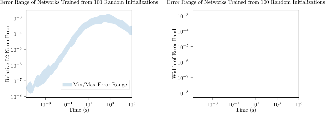
6.8.2 Collisional-Radiative Model↩︎
For the CR charge state model (3.2), we, again, trained networks from 100 random parameter initializations. In 24, the left plot shows the mean relative error over time 37 on a test dataset of 4096 samples, while the right plot shows the width of the error band over time. The width of the error band generally stays on the same scale as the error.
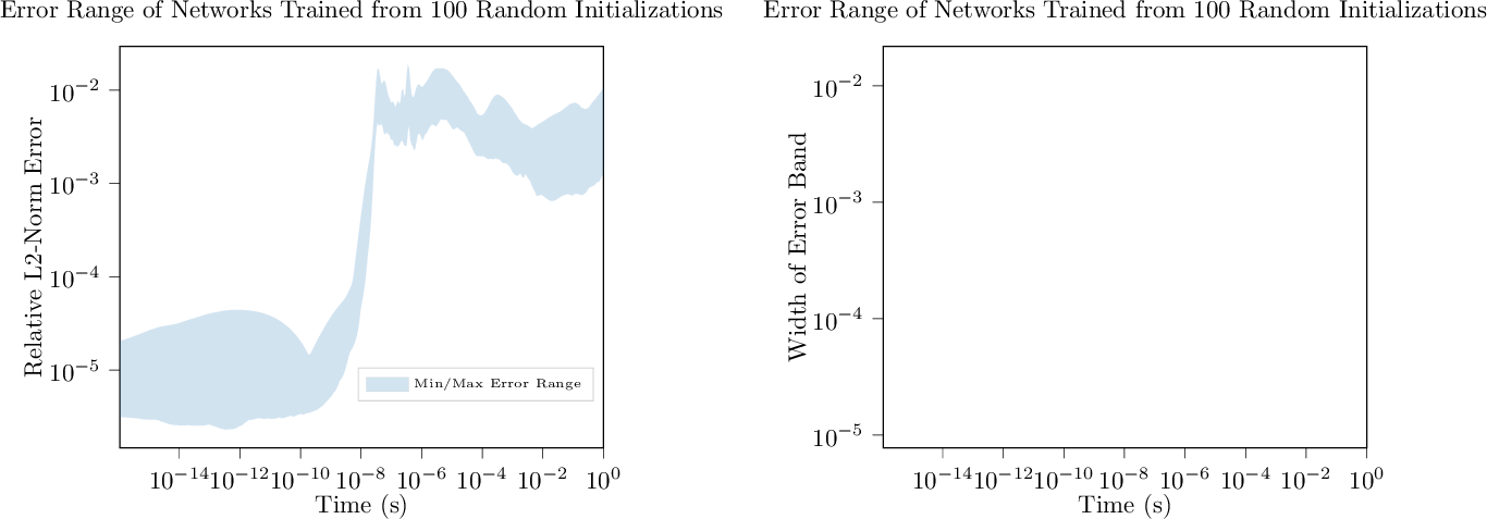
For the full CR model (3.2), we trained networks from 15 random parameter initializations. Fewer networks were trained because the networks are much more costly to train on this problem. In 25, the left plot shows the mean relative error over time 37 on a test dataset of 2500 samples, while the right plot shows the width of the error band over time. The width of the error band generally stays on the same scale as the error.

6.8.3 Allen-Cahn PDE↩︎
For the Allen-Cahn PDE (3.3), we trained networks from 100 random parameter initializations. In 26, the left plot shows the mean relative error over time 37 on a test dataset of 200 samples, while the right plot shows the width of the error band over time. The width of the error band generally stays on the same scale as the error.

6.8.4 Cahn-Hilliard PDE↩︎
For the Cahn-Hilliard PDE (3.4), we trained networks from 100 random parameter initializations. In 27, the left plot shows the mean relative error over time 37 on a test dataset of 200 samples, while the right plot shows the width of the error band over time. The width of the error band generally stays on the same scale as the error.
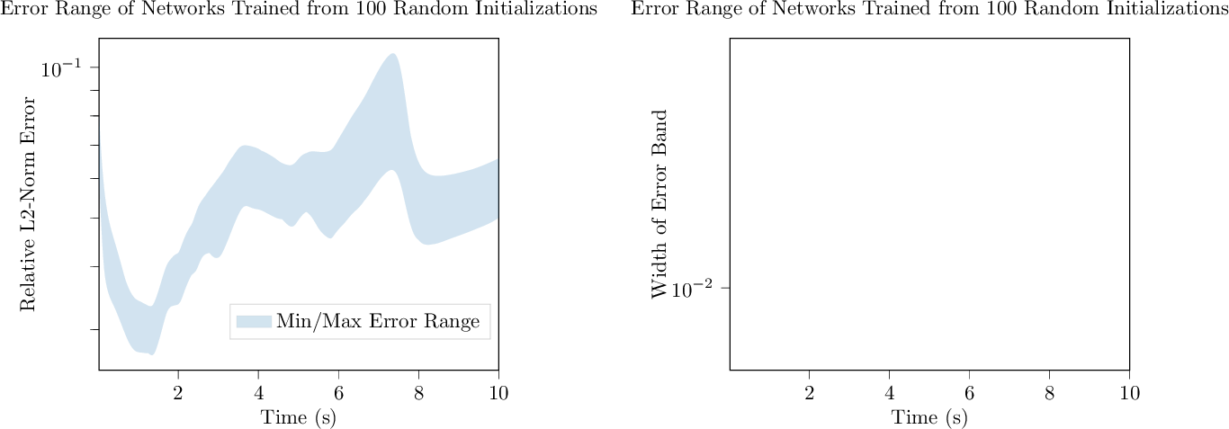
References↩︎
Refer to [28] for the definition of maximal interval of existence of the solution.↩︎
We were not aware of their work during the development of
LiLaN. Our inspiration is kernel methods as discussed at the end of 1.↩︎\(\boldsymbol{f}\left( \boldsymbol{x},\;\mathbf{p} \right)\) is globally Lipschitz continuous if there exists a non-negative constant \(M\) such that \(\left\| \boldsymbol{f}(\boldsymbol{x}_1,\;\mathbf{p}_1)-\boldsymbol{f}(\boldsymbol{x}_2,\;\mathbf{p}_2) \right\|_2\leq M\left\| \mathbf{r}_1-\mathbf{r_2} \right\|_2,\forall \mathbf{r}_1,\mathbf{r}_2\in \mathbb{R}^{n_x+n_p}\), where \(\mathbf{r}_1=[\boldsymbol{x}_1,\;\mathbf{p}_1]\) and \(\mathbf{r}_2=[\boldsymbol{x}_2,\;\mathbf{p}_2]\).↩︎
Non-uniqueness here implies that there are infinitely many choices for functions \({\boldsymbol{l}}\), \(\boldsymbol{b}\), \(\mathbf{g}\), \(\boldsymbol{h}\) for which ?? holds true.↩︎
When \({\boldsymbol{l}}\) satisfies this condition we say that \({\boldsymbol{l}}\) is a topological embedding of \(\mathbb{R}^{n_x}\) into \(\mathbb{R}^m\)[35].↩︎