Keywords. modulating function, infinite-dimensional systems, partial differential equations, boundary control, state feedback, state reconstruction

Mathematics Subject Classification (2020). 93C25, 93B53, 93B07, 93B28

1 Introduction↩︎

The modulating function approach reconstructs selected components of the state by convolving the input and output with suitably chosen precomputed functions. More precisely, for a linear system \[\begin{align} \dot{x}(t)&=Ax(t)+Bu(t),\\ y(t)&=Cx(t)+Du(t), \end{align}\label{eq:ABCDfin}\tag{1}\] \(A\in\mathbb{R}^{n\times n}\), \(B\in\mathbb{R}^{n\times m}\), \(C\in\mathbb{R}^{p\times n}\), \(D\in\mathbb{R}^{p\times m}\), the approach consists of constructing, for given \(T>0\) and \(\varphi_0\in\mathbb{R}^n\), functions \(\mu:[0,T]\to\mathbb{R}^m\) and \(\eta:[0,T]\to\mathbb{R}^p\) such that every trajectory of 1 satisfies \[\forall\,t\geq T: \quad \varphi_0^\top x(t)=\int_{0}^T u(t-\tau)^\top \mu(\tau)-y(t-\tau)^\top \eta(\tau){\rm d}\tau. \label{eq:movhor95fin}\tag{2}\] Thus, \(\varphi_0^\top x(t)\), which represents a component of \(x(t)\) in the direction determined by \(\varphi_0\), can be reconstructed from the input and output on the moving horizon \([t-T,t]\) by evaluating the integral in 2 . A straightforward integration by parts shows that suitable functions \(\mu\) and \(\eta\) are obtained by solving the following null-control problem for the adjoint system \[\begin{align} \dot{\varphi}(t)&=A^\top \varphi(t)+C^\top \eta(t),\qquad \varphi(0)=\varphi_0,\;\;\;\varphi(T)=0,\\ \mu(t)&=B^\top \varphi(t)+D^\top\eta(t). \end{align}\label{eq:ABCDfin95dualnull}\tag{3}\] Then \(\mu\) and \(\eta\) satisfy the reconstruction identity 2 . Classical systems theory implies that the control problem 3 is solvable if the system 1 is observable. Moreover, the solution of 3 can be computed offline, so that the online reconstruction requires only the evaluation of the convolution integrals. This approach can be used for two purposes:

(a) State estimation: By choosing a linearly independent family \((\varphi_{01},\ldots,\varphi_{0n})\) and determining corresponding null controls \(\eta_1,\ldots,\eta_n\) and outputs \(\mu_1,\ldots,\mu_n\) of the adjoint system, we can reconstruct the scalars \(\varphi_{0i}^\top x(t)\) for \(i=1,\ldots,n\). These values then allow us to determine \(x(t)\). If only \(N\leq n\) such null controls are used, we obtain the orthogonal projection, and hence the best approximation, of \(x(t)\) onto the \(N\)-dimensional subspace \(\operatorname{span}(\varphi_{01},\ldots,\varphi_{0N})\). The reconstruction is particularly simple if the initial values of the adjoint null-control problems form an orthonormal family.

(b) State feedback: Here, the aim is to realise the state feedback \(u(t)=Fx(t)\), \(F\in\mathbb{R}^{m\times n}\), using only the measured input and output. To achieve this, we solve \(m\) null control problems for the adjoint system, where the initial values \(\varphi_{01},\ldots,\varphi_{0m}\in\mathbb{R}^n\) are the transposes of the row vectors of \(F\). Then 2 shows that the moving-horizon integrals of the input and output of 1 yield \[\left(\begin{smallmatrix} \varphi_{01}^\top x(t)\\[-1.2mm]\vdots\\ \varphi_{0m}^\top x(t) \end{smallmatrix}\right)=\left[\begin{smallmatrix} \varphi_{01}^\top\\[-1.2mm]\vdots\\ \varphi_{0m}^\top \end{smallmatrix}\right]x(t)=Fx(t).\]

Although the modulating-function approach is relatively straightforward for finite-dimensional systems, its extension to infinite-dimensional systems involves substantial difficulties, particularly in the presence of boundary control or observation. To cover a broad class of infinite-dimensional linear systems, we employ the system-node framework developed by Staffans in [1] and related publications. Such systems are described by \[\left(\begin{smallmatrix}\dot{x}(t)\\y(t)\end{smallmatrix}\right) = \left[\begin{smallmatrix}A\&B\\[-1mm]\\C\&D\end{smallmatrix}\right] \left(\begin{smallmatrix}{x}(t)\\u(t)\end{smallmatrix}\right),\label{eq:ODEnode}\tag{4}\] where \(A\&B:X\times U\supset\operatorname{dom}(A\&B)\to X\) and \(C\&D:X\times U\supset\operatorname{dom}(C\&D)\to Y\) are linear operators whose precise properties are specified in the next section. The symbols \(\&\) indicate that the domains of these operators need not be Cartesian products of subspaces of \(X\) and \(U\). Although the comprehensive theory of system nodes developed in [1] contains only a few examples involving partial differential equations, many such systems can be incorporated naturally into this framework, including systems on multidimensional spatial domains. Examples include systems governed by the wave equation, advection–diffusion equations, Maxwell’s equations, the Oseen equations, and the Euler–Bernoulli and Timoshenko beam equations [2]–[5].

A further important advantage is that the class of system nodes is closed under adjunction, which allows us to formulate an infinite-dimensional counterpart of the null-control problem 3 .

The objective of this article is to develop a modulating-function framework for infinite-dimensional linear systems described by system nodes, with particular emphasis on state estimation and the realisation of state feedback using only input and output data. For state estimation, we show that, for \(\varphi_0\in X\) and suitable functions \(\mu\in L^2([0,T];U)\) and \(\eta\in L^2([0,T];Y)\) arising from a null-control problem for the adjoint system, \[\forall\,t\geq T: \quad \langle x(t),\varphi_0\rangle_X=\int_{0}^T \langle u(t-\tau),\mu(\tau)\rangle_U -\langle y(t-\tau),\eta(\tau)\rangle_Y{\rm d}\tau. \label{eq:movhor95inf}\tag{5}\] Applying this identity simultaneously to initial values \(\varphi_{01},\ldots,\varphi_{0k}\) of the adjoint null-control problem yields the orthogonal projection of \(x(t)\) onto \(\operatorname{span}(\varphi_{01},\ldots,\varphi_{0k})\).

The application to state feedback becomes more involved when the feedback operator is unbounded. More precisely, we consider feedback laws of the form \(u=Fx\), where \(F\) maps an intermediate space \(\mathcal{V}\) between \(\operatorname{dom}(A)\) and \(X\) into the input space \(U\). In this setting, \(U\) is assumed to be finite-dimensional. For \(U=\mathbb{R}^m\), the feedback operator \(F\) can be represented by an \(m\)-tuple of elements of \(\mathcal{V}^\prime\), where \(\mathcal{V}^\prime\) denotes the dual of \(\mathcal{V}\) with respect to the pivot space \(X\). The space \(\mathcal{V}^\prime\) may be regarded as an extension of the state space of the adjoint system. We therefore seek inputs \(\eta_i\) that drive the adjoint system, formally initialised at \(\varphi(0)=F_i\), to zero in an appropriate sense. Such null controls need not exist within a classical function-space setting. This motivates the extension of the solution theory for system nodes to distributional inputs and trajectories. In this distributional setting, the reconstruction identity 5 requires a more general interpretation. More precisely, the action of \(F_i\) on \(x(t)\) is represented by convolutions of the distributions \(\eta_i\) and \(\mu_i\) with the input \(u\) and the output \(y\), rather than by moving-horizon \(L^2\)-inner products. The treatment of unbounded feedback operators is particularly important because it allows feedback laws involving spatial point evaluations for systems governed by partial differential equations.

We do not assume that the system or its adjoint is well-posed. Although well-posedness considerably simplifies the analysis, it restricts the class of systems under consideration, and suitable well-posedness criteria are not available for all systems of practical interest. By allowing non-well-posed system nodes, our framework applies to a broader class of boundary-controlled partial differential equations. This generality, together with the treatment of unbounded feedback operators, requires a more extensive theoretical framework.

The remainder of this article is organised as follows. Section 2 introduces the notation, function spaces, and operator-theoretic framework used throughout the article. In Section 3, we recall the basic theory of system nodes and develop a distributional solution framework. Section 4 considers the adjoint system and its systems-theoretic properties and contains our main result on distributional partial-state reconstruction. Section 5 applies this result to state estimation, while Section 6 addresses the implementation of state feedback. Section 7 presents two examples. The first concerns the construction of an exponentially stabilising feedback law for a vibrating string with boundary force control and an interior velocity measurement. The second considers state estimation for a reaction–diffusion equation on a two-dimensional spatial domain with Dirichlet boundary control and Neumann boundary observation.

We conclude this introduction with a brief overview of the literature on the modulating-function approach. The method originates from the work of Shinbrot [6]. Its basic idea is to use modulating functions to transform linear and certain nonlinear ordinary differential equations into algebraic equations, thereby enabling the application of regression methods to the estimation of unknown system parameters. In the following decades, the modulating-function method was applied to parameter estimation for increasingly broad classes of systems. Of particular relevance to the present work are the early applications to systems governed by partial differential equations by Perdreauville and Goodson [7] and, subsequently, by Fairman and Shen [8]. Subsequent developments largely focused on finite-dimensional systems and, in particular, on the choice of suitable modulating functions. The modulating-function method was first applied to state estimation for finite-dimensional systems in [9], [10], where modulating functions with non-zero boundary values were employed. Since the original work of Shinbrot, modulating functions have typically been required only to satisfy suitable homogeneous boundary conditions and differentiability assumptions, leaving their precise shape as a degree of freedom.

In [11], Fischer and Deutscher developed a modulating-function-based fault-detection framework for systems governed by partial differential equations. Their approach transforms the differential equation into an algebraic relation that gives rise to a kernel equation, whose solution determines the modulating function. This approach was subsequently used in [12] to construct a state estimator for parabolic partial differential equations. The resulting estimate is given in terms of the coefficients of a truncated series expansion of the distributed state. The approach was extended to coupled parabolic systems in [13] and to parabolic systems with certain nonlinear reaction terms in [14]. To the best of our knowledge, a systematic and unified modulating-function framework for infinite-dimensional systems that accommodates boundary control and unbounded feedback operators has not yet been developed.

2 Notation, function spaces, and operator-theoretic preliminaries↩︎

The sets of positive and non-negative integers are denoted by \(\mathbb{N}\) and \(\mathbb{N}_0\), respectively. Unless stated otherwise, all Hilbert spaces considered in this article are real. By complexification, the results can also be formulated for complex Hilbert spaces. The norm on \(X\) is denoted by \(\|\cdot\|_X\), or simply by \(\|\cdot\|\) if the underlying space is clear from the context. The identity operator on \(X\) is denoted by \(I_X\), or simply by \(I\).

The topological dual of \(X\) is denoted by \(X^\prime\), and the corresponding duality pairing by \(\langle\cdot,\cdot\rangle_{X^\prime,X}\). Using the reflexivity of \(X\), we set \(\langle x,x^\prime\rangle_{X,X^\prime}\mathrel{\vcenter{:}}= \langle x^\prime,x\rangle_{X^\prime,X}\) for all \(x\in X\) and \(x^\prime\in X^\prime\).

The space of bounded linear operators from \(X\) to \(Y\) is denoted by \(L(X,Y)\), and we write \(L(X)\mathrel{\vcenter{:}}= L(X,X)\). The domain \(\operatorname{dom}A\) of a possibly unbounded linear operator \(A:X\supset\operatorname{dom}A\to Y\) is endowed with the graph norm \[\|x\|_{\operatorname{dom}A}\mathrel{\vcenter{:}}= \big(\|x\|_{X}^2+\|Ax\|_{Y}^2\big)^{1/2}.\] For a densely defined linear operator \(A:X\supset\operatorname{dom}A\to Y\), its dual operator \(A^\prime:Y^\prime\supset\operatorname{dom}A^\prime\to X^\prime\) is defined by \[\operatorname{dom}A^\prime=\left\{ y^\prime\in Y^\prime \left\vert\vphantom{y^\prime\in Y^\prime} \exists\, z^\prime\in X^\prime\text{ s.t.\;}\forall\,x\in\operatorname{dom}A:\;\langle Ax,y^\prime\rangle_{Y,Y^\prime}=\langle z^\prime,x\rangle_{X^\prime,X} \right.\right\}.\] For each \(y^\prime\in\operatorname{dom}A^\prime\), the element \(z^\prime\in X^\prime\) in the above definition is uniquely determined, and we set \(A^\prime y^\prime\mathrel{\vcenter{:}}= z^\prime\). If \(X\) and \(Y\) are identified with their dual spaces, the dual operator is called the adjoint of \(A\) and is denoted by \(A^*:Y\supset\operatorname{dom}A^*\to X\).

For Lebesgue and Sobolev spaces, we follow the notation of Adams [15]. For spaces of functions taking values in a Hilbert space \(X\), the target space is indicated after a semicolon. For example, the space of \(p\)-integrable \(X\)-valued functions on \(\Omega\) is denoted by \(L^p(\Omega;X)\).

For \(T>0\) and \(k\in\mathbb{N}\), we define \[\begin{align} H^k_{0l}([0,T];X) &\mathrel{\vcenter{:}}= \left\{ v\in H^k([0,T];X) \left\vert\vphantom{v\in H^k([0,T];X)} v(0)= \cdots =\tfrac{\mathrm{d}^{k-1}}{\mathrm{d}t^{k-1}}v(0) = 0 \right.\right\},\tag{6}\\ H^k_{0r}([0,T];X) &\mathrel{\vcenter{:}}= \left\{ v\in H^k([0,T];X) \left\vert\vphantom{v\in H^k([0,T];X)} v(T)= \cdots =\tfrac{\mathrm{d}^{k-1}}{\mathrm{d}t^{k-1}}v(T) = 0 \right.\right\}.\tag{7} \end{align}\] These spaces will be used throughout the article. Both are closed subspaces of \(H^k([0,T];X)\) and hence Hilbert spaces with respect to the norm inherited from \(H^k([0,T];X)\).

Using \(L^2([0,T];X)\) as the pivot space, we define the corresponding negative-order spaces by \[H^{-k}_{0l}([0,T];X) \mathrel{\vcenter{:}}= H^k_{0r}([0,T];X)^\prime,\qquad H^{-k}_{0r}([0,T];X) \mathrel{\vcenter{:}}= H^k_{0l}([0,T];X)^\prime. \label{eq:H-kl}\tag{8}\] For \(k=0\), we set \[H^{0}_{0l}([0,T];X)\mathrel{\vcenter{:}}= L^2([0,T];X)=:H^{0}_{0r}([0,T];X).\] The Dirac distribution \(\delta\in H^{-1}_{0l}([0,T])\) is defined by \[\langle\delta,w\rangle_{H^{-1}_{0l}([0,T]),H^{1}_{0r}([0,T])} =w(0) \qquad \forall\,w\in H^{1}_{0r}([0,T]).\] For \(k\geq0\), the left derivative \[\big(\tfrac{\mathrm{d}}{\mathrm{d}t}\big)_l: H^{-k}_{0l}([0,T];X)\to H^{-k-1}_{0l}([0,T];X)\] is defined as the negative dual of the right derivative, that is, \[\begin{align} \label{eq:l2nder} \begin{aligned} \left\langle \big(\tfrac{\mathrm{d}}{\mathrm{d}t}\big)_l v, w\right\rangle_{H^{-k-1}_{0l}([0,T];X),H^{k+1}_{0r}([0,T];X)} &\mathrel{\vcenter{:}}= -\left\langle v,\tfrac{\mathrm{d}}{\mathrm{d}t}w\right\rangle_{H^{-k}_{0l}([0,T];X),H^{k}_{0r}([0,T];X)} \\ &\forall\,v\in H^{-k}_{0l}([0,T];X),\, w\in H^{k+1}_{0r}([0,T];X). \end{aligned} \end{align}\tag{9}\] For \(v\in H^{k}_{0l}([0,T];X)\), \(k\in\mathbb{N}\), the left derivative agrees with the conventional weak derivative. Consequently, for every \(k\in\mathbb{Z}\), \(\big(\tfrac{\mathrm{d}}{\mathrm{d}t}\big)_l\) is a bounded bijective operator from \(H^{k}_{0l}([0,T];X)\) onto \(H^{k-1}_{0l}([0,T];X)\). The right derivative \[\big(\tfrac{\mathrm{d}}{\mathrm{d}t}\big)_r: H^{k}_{0r}([0,T];X)\to H^{k-1}_{0r}([0,T];X), \qquad k\in\mathbb{Z},\] is defined analogously.

For \(\tau\in[0,T]\), the \(\tau\)-right shift operator \(S_{r,\tau}\in L(L^2([0,T];X))\) maps \(v\in L^2([0,T];X)\) to the function \(S_{r,\tau}v\) defined by \[(S_{r,\tau}v)(t)= \begin{cases} 0,&t\in[0,\tau),\\ v(t-\tau),&t\in[\tau,T], \end{cases}\] for almost every \(t\in[0,T]\). Its restriction defines a bounded operator on \(H^k_{0l}([0,T];X)\). Analogously, the \(\tau\)-left shift operator \(S_{l,\tau}\) defines a bounded operator on \(H^k_{0r}([0,T];X)\). For \(k\geq0\), the \(\tau\)-right shift on \(H^{-k}_{0l}([0,T];X)\) is defined as the dual of the \(\tau\)-left shift on \(H^{k}_{0r}([0,T];X)\). With this definition, the right shift on \(L^2([0,T];X)\) extends to the spaces \(H^{-k}_{0l}([0,T];X)\).

Let \(A\in L(X,Y)\) and \(k\in\mathbb{N}\). For \(w\in H^{k}_{0l}([0,T];X)\), the pointwise application \(Aw\mathrel{\vcenter{:}}= \big(t\mapsto Aw(t)\big)\) belongs to \(H^{k}_{0l}([0,T];Y)\). Likewise, \(Aw\in H^{k}_{0r}([0,T];Y)\) whenever \(w\in H^{k}_{0r}([0,T];X)\). The pointwise application of \(A\) to an element \(v\in H^{-k}_{0l}([0,T];X)\) is defined by \[\begin{gather} \label{eq:Apointwl} \langle A v, w\rangle_{H^{-k}_{0l}([0,T];Y),H^k_{0r}([0,T];Y)} \mathrel{\vcenter{:}}= \langle v, A^* w\rangle_{H^{-k}_{0l}([0,T];X),H^k_{0r}([0,T];X)} \\ \forall\,v\in H^{-k}_{0l}([0,T];X),\, w\in H^k_{0r}([0,T];Y). \end{gather}\tag{10}\] The pointwise application of \(A\) to elements of \(H^{-k}_{0r}([0,T];X)\) is defined analogously. With these definitions, the pointwise application of \(A\) commutes with both the left and the right derivative, that is, \[\big(\tfrac{{\rm d}}{{\rm d}t}\big)_lA =A\big(\tfrac{{\rm d}}{{\rm d}t}\big)_l, \qquad \big(\tfrac{{\rm d}}{{\rm d}t}\big)_rA =A\big(\tfrac{{\rm d}}{{\rm d}t}\big)_r.\]

We next introduce function spaces on the infinite time horizon. The elements of the spaces defined above can be canonically identified with distributions in the sense of Schwartz. More precisely, an element of \(H^{-k}_{0l}([0,T];X)\), \(k\in\mathbb{N}\), defines a distribution on \((-\infty,T)\) supported in \([0,T)\) by \[\langle v,\psi\rangle \mathrel{\vcenter{:}}= \langle v,\psi|_{[0,T]}\rangle_{H^{-k}_{0l}([0,T];X),H^k_{0r}([0,T];X)}, \qquad \psi\in C^\infty_0((-\infty,T);X).\] The elements of \(H^{-k}_{0r}([0,T];X)\) are identified analogously with distributions on \((0,\infty)\) supported in \((0,T]\). Elements of non-negative order are regarded as regular distributions.

Accordingly, the support of an element of any of these spaces is understood as its distributional support in the sense of Schwartz; see [16]. Equivalently, for \(v\in H^{-k}_{0l}([0,T];X)\), a relatively open set \(J\subset[0,T)\) is disjoint from \(\mathop{\mathrm{supp}}v\) if and only if \[\langle v,w\rangle_{H^{-k}_{0l}([0,T];X),H^k_{0r}([0,T];X)} =0\] for every \(w\in H^k_{0r}([0,T];X)\) with \(\mathop{\mathrm{supp}}w\subset J\). The analogous characterisation applies to elements of \(H^{-k}_{0r}([0,T];X)\).

For \(k\in\mathbb{N}_0\), the space \(H^k_{0,\mathrm{loc}}(\mathbb{R}_{\ge0};X)\) consists of all \(v\in L^2_{\mathrm{loc}}(\mathbb{R}_{\ge0};X)\) such that, for every \(T>0\), the restriction of \(v\) to \([0,T]\) belongs to \(H^k_{0l}([0,T];X)\). We equip this space with the locally convex topology generated by the seminorms given by the \(H^k_{0l}([0,T];X)\)-norms of these restrictions; see [16].

To define \(H^{-k}_{0,\mathrm{loc}}(\mathbb{R}_{\geq0};X)\) for \(k>0\), let \(0<T_1<T_2\). Extension by zero on \([T_1,T_2]\) defines a continuous embedding of \(H_{0r}^k([0,T_1];X)\) into \(H_{0r}^k([0,T_2];X)\). Its dual defines the restriction operator from \(H_{0l}^{-k}([0,T_2];X)\) to \(H_{0l}^{-k}([0,T_1];X)\). An element \(v\in H_{0,\mathrm{loc}}^{-k}(\mathbb{R}_{\geq0};X)\) is a family \((v_T)_{T>0}\) with \(v_T\in H^{-k}_{0l}([0,T];X)\) such that, whenever \(0<T_1<T_2\), the restriction of \(v_{T_2}\) to \([0,T_1]\) equals \(v_{T_1}\). We equip this space with the locally convex topology generated by the seminorms \[v\mapsto\|v_T\|_{H^{-k}_{0l}([0,T];X)}, \qquad T>0.\] The support of \(v=(v_T)_{T>0}\) is defined by \[\mathop{\mathrm{supp}}v \mathrel{\vcenter{:}}= \bigcup_{T>0} \big(\mathop{\mathrm{supp}}v_T\cap[0,T)\big).\] With these definitions, \(H_{0,\mathrm{loc}}^{0}(\mathbb{R}_{\geq0};X)\) is identified with \(L^2_{\mathrm{loc}}(\mathbb{R}_{\geq0};X)\).

The left derivative \(\left(\frac{{\rm d}}{{\rm d}t}\right)_l\) extends naturally to \(H_{0,\mathrm{loc}}^{k}(\mathbb{R}_{\ge0};X)\) for every \(k\in\mathbb{Z}\). It defines a continuous bijection from \(H_{0,\mathrm{loc}}^{k}(\mathbb{R}_{\ge0};X)\) onto \(H_{0,\mathrm{loc}}^{k-1}(\mathbb{R}_{\ge0};X)\) with continuous inverse. Similarly, the \(\tau\)-right shift defines a continuous operator on \(H_{0,\mathrm{loc}}^{k}(\mathbb{R}_{\ge0};X)\) for every \(k\in\mathbb{Z}\), as follows from its boundedness on finite time intervals.

We conclude these preliminaries by introducing convolution. For \(v,w\in L^{2}_{\mathrm{loc}}(\mathbb{R}_{\ge0};X)\), we define their convolution \(v\ast w\in L^{2}_{\mathrm{loc}}(\mathbb{R}_{\ge0})\) by \[(v\ast w)(t)=\int_0^t \langle v(\tau),w(t-\tau)\rangle_X\,{\rm d}\tau.\] The convolution \(v\ast w\) is continuous. Moreover, convolution is bilinear and commutative and defines a continuous mapping from \(L^{2}_{\mathrm{loc}}(\mathbb{R}_{\ge0};X)\times L^{2}_{\mathrm{loc}}(\mathbb{R}_{\ge0};X)\) to \(L^{2}_{\mathrm{loc}}(\mathbb{R}_{\ge0})\). Its restriction to \([0,T]\) depends only on the restrictions of \(v\) and \(w\) to \([0,T]\).

If \(v\in H^{1}_{0,\mathrm{loc}}(\mathbb{R}_{\ge0};X)\) and \(w\in L^{2}_{\mathrm{loc}}(\mathbb{R}_{\ge0};X)\), then \(v\ast w\in H^{1}_{0,\mathrm{loc}}(\mathbb{R}_{\ge0})\) and \[\big(\tfrac{{\rm d}}{{\rm d}t}\big)_l(v\ast w) = \left(\big(\tfrac{{\rm d}}{{\rm d}t}\big)_lv\right)\ast w.\] Since the left derivative is a linear homeomorphism from \(H^{k}_{0,\mathrm{loc}}(\mathbb{R}_{\geq0};X)\) onto \(H^{k-1}_{0,\mathrm{loc}}(\mathbb{R}_{\geq0};X)\) for every \(k\in\mathbb{Z}\), convolution extends uniquely to a continuous bilinear mapping \[\ast: H^{k_1}_{0,\mathrm{loc}}(\mathbb{R}_{\geq0};X) \times H^{k_2}_{0,\mathrm{loc}}(\mathbb{R}_{\geq0};X) \to H^{k_1+k_2}_{0,\mathrm{loc}}(\mathbb{R}_{\geq0})\] defined by \[\begin{align} \big(\tfrac{{\rm d}}{{\rm d}t}\big)_l^{k_1+k_2}(v\ast w) &= \left(\big(\tfrac{{\rm d}}{{\rm d}t}\big)_l^{k_1}v\right) \ast \left(\big(\tfrac{{\rm d}}{{\rm d}t}\big)_l^{k_2}w\right) \end{align} \label{eq:convrule}\tag{11}\] for all \(k_1,k_2\in\mathbb{Z}\), \(v\in H^{k_1}_{0,\mathrm{loc}}(\mathbb{R}_{\geq0};X)\), and \(w\in H^{k_2}_{0,\mathrm{loc}}(\mathbb{R}_{\geq0};X)\). Here, negative powers of the left derivative denote powers of its continuous inverse. The convolution \(\varphi\ast v\in H^{k_1+k_2}_{0,\mathrm{loc}}(\mathbb{R}_{\geq0};X)\) of a scalar element \(\varphi\in H^{k_1}_{0,\mathrm{loc}}(\mathbb{R}_{\geq0})\) and an \(X\)-valued element \(v\in H^{k_2}_{0,\mathrm{loc}}(\mathbb{R}_{\geq0};X)\) is defined analogously.

3 System nodes and trajectories↩︎

Let \(X\), \(U\), and \(Y\) be Hilbert spaces, and let \(A\&B:\operatorname{dom}(A\&B)\subset X\times U\to X\) and \(C\&D:\operatorname{dom}(C\&D)\subset X\times U\to Y\) be linear operators. In this section, we recall the basic concepts required for systems of the form 4 . In contrast to the finite-dimensional case, the operators \(A\&B\) and \(C\&D\) need not decompose into separate components associated with the state and the input. This feature is essential for the treatment of boundary control systems governed by partial differential equations. The autonomous dynamics, corresponding to the trivial input \(u\equiv0\), are determined by the so-called main operator \(A\colon\operatorname{dom}(A)\subset X\to X\), where \(\operatorname{dom}(A)\mathrel{\vcenter{:}}=\left\{ x\in X \left\vert\vphantom{x\in X} \left(\begin{smallmatrix}x\\0\end{smallmatrix}\right)\in\operatorname{dom}(A\&B) \right.\right\}\) and \(Ax\mathrel{\vcenter{:}}= A\&B\left(\begin{smallmatrix}x\\0\end{smallmatrix}\right)\) for all \(x\in\operatorname{dom}(A)\).

These properties imply that \(S\) is closed and that \(\operatorname{dom}(S)=\operatorname{dom}(A\&B)\).

We next introduce classical and generalised trajectories of 4 . The space \(C(\mathbb{R}_{\geq0};X)\) is equipped with the locally convex topology generated by the seminorms given by the maximum norm on intervals \([0,T]\), \(T>0\).

Any operator \(A\&B\) satisfying conditions [def:sysnodea], [def:sysnodec], and [def:sysnoded] of Definition 1 can be regarded as a system node on \((X,U,\{0\})\). Accordingly, we also speak of classical and generalised trajectories \((x,u)\) of \[\begin{align} \label{eq:ODE} \dot{x}=A\&B\left(\begin{smallmatrix}x\\u\end{smallmatrix}\right). \end{align}\tag{12}\]

We next recall a solvability result from [1]. In addition to sufficient regularity of the input, it requires compatibility between the initial state and the initial input value in the sense that the corresponding pair belongs to \(\operatorname{dom}(A\&B)\). For boundary control systems, this means that the boundary value of the prescribed initial state is consistent with the input at \(t=0\).

To formulate further results on the existence and regularity of trajectories, it is useful to separate \(A\&B\) into operators associated with the state and the input, as is customary in the theory of infinite-dimensional systems; see, for instance, [17]. This separation requires the introduction of extrapolation spaces containing \(X\) as a continuously and densely embedded subspace.

We collect some further properties of classical and generalised trajectories.

The output expression
$$y(t)=C\&D\left(\begin{smallmatrix}x(t)\\u(t)\end{smallmatrix}\right)$$
is not necessarily defined pointwise. However, [@Staffans2005] shows
that the second time primitive $$g
\mathrel{\vcenter{:}}=
\int_0^\cdot(\cdot-\tau)
\left(\begin{smallmatrix}x(\tau)\\u(\tau)\end{smallmatrix}\right)\,{\rm d}\tau$$
belongs to $$C(\mathbb{R}_{\geq0};\operatorname{dom}(A\&B))
\subset
L^2_{\mathrm{loc}}(\mathbb{R}_{\geq0};\operatorname{dom}(A\&B)).$$
We may therefore define the distributional output by $$y
\mathrel{\vcenter{:}}=
\big(\tfrac{{\rm d}}{{\rm d}t}\big)_l^2
\big(C\&Dg\big)
=
C\&D\left(\begin{smallmatrix}x\\u\end{smallmatrix}\right)
\in H^{-2}_{0,\mathrm{loc}}(\mathbb{R}_{\geq0};Y),
\label{eq:ydef}$$ {#eq:eq:ydef}  where the final equality follows
from the pointwise application of bounded operators introduced in
@eq:eq:Apointwl .

Consequently, a triple $$(x,u,y)\in
C(\mathbb{R}_{\geq0};X)
\times L^2_{\mathrm{loc}}(\mathbb{R}_{\geq0};U)
\times L^2_{\mathrm{loc}}(\mathbb{R}_{\geq0};Y)$$ is a generalised
trajectory of @eq:eq:ODEnode if and only if $(x,u)$ is a generalised
trajectory of @eq:eq:ODE and the distribution defined in @eq:eq:ydef
is represented by the $L^2_{\mathrm{loc}}$-function $y$.

Remark 5 motivates the introduction of the continuous input-to-state map \[\begin{align} \mathfrak S:\quad L^2_{\mathrm{loc}}(\mathbb{R}_{\geq0};U) &\to L^2_{\mathrm{loc}}(\mathbb{R}_{\geq0};X_{-1}), \label{eq:genISmap}\\ u&\mapsto \int_0^\cdot \mathfrak A_{-1}(\cdot-\tau)Bu(\tau)\,{\rm d}\tau. \nonumber \end{align}\tag{15}\] It maps an input to the corresponding state trajectory with zero initial state. For every \(T>0\), the restriction of \(\mathfrak Su\) to \([0,T]\) belongs to \(C([0,T];X_{-1})\). We nevertheless use \(L^2_{\mathrm{loc}}(\mathbb{R}_{\geq0};X_{-1})\) as the codomain in 15 , since this allows us to incorporate \(\mathfrak S\) into the Sobolev-space framework introduced above.

Remark 5 [rem:sols2] further implies that the mapping \[u\mapsto\left(\begin{smallmatrix}\mathfrak Su\\u\end{smallmatrix}\right) \label{eq:uA38B}\tag{16}\] is continuous from \(L^2_{\mathrm{loc}}(\mathbb{R}_{\geq0};U)\) to \(H^{-2}_{0,\mathrm{loc}}(\mathbb{R}_{\geq0};\operatorname{dom}(A\&B))\).

In this notation, well-posedness is equivalent to the following three properties: the map \(\mathfrak C_0\) takes values in \(L^2_{\mathrm{loc}}(\mathbb{R}_{\geq0};Y)\), the map \(\mathfrak S\) takes values in \(C(\mathbb{R}_{\geq0};X)\), and \[u\mapsto C\&D\left(\begin{smallmatrix}\mathfrak Su\\u\end{smallmatrix}\right)\] maps \(L^2_{\mathrm{loc}}(\mathbb{R}_{\geq0};U)\) into \(L^2_{\mathrm{loc}}(\mathbb{R}_{\geq0};Y)\).

It follows from Remark 5 that \[(x,u,y)\in C(\mathbb{R}_{\geq0};X) \times L^2_{\mathrm{loc}}(\mathbb{R}_{\geq0};U) \times L^2_{\mathrm{loc}}(\mathbb{R}_{\geq0};Y)\] is a generalised trajectory of 4 if and only if there exists some \(x_0\in X\) such that \[x=\mathfrak A(\cdot)x_0+\mathfrak Su, \qquad y=\mathfrak C_0x_0+C\&D\left(\begin{smallmatrix}\mathfrak Su\\u\end{smallmatrix}\right).\] This characterisation provides the basis for the distributional extension of the trajectory concept.

By shift invariance, \[\forall\,u\in C_0^\infty(\mathbb{R}_{>0};U):\quad \mathfrak S\big(\tfrac{{\rm d}}{{\rm d}t}\big)_lu = \big(\tfrac{{\rm d}}{{\rm d}t}\big)_l\mathfrak Su.\] Since \(C_0^\infty(\mathbb{R}_{>0};U)\) is dense in \(H^1_{0,\mathrm{loc}}(\mathbb{R}_{\geq0};U)\), this identity extends by continuity to every \(u\in H^1_{0,\mathrm{loc}}(\mathbb{R}_{\geq0};U)\). In particular, \[\mathfrak Su\in H^1_{0,\mathrm{loc}}(\mathbb{R}_{\geq0};X_{-1})\] and \[\mathfrak S\big(\tfrac{{\rm d}}{{\rm d}t}\big)_lu = \big(\tfrac{{\rm d}}{{\rm d}t}\big)_l\mathfrak Su.\] Iteration shows that \(\mathfrak S\) restricts to a continuous operator from \(H^k_{0,\mathrm{loc}}(\mathbb{R}_{\geq0};U)\) to \(H^k_{0,\mathrm{loc}}(\mathbb{R}_{\geq0};X_{-1})\) for every \(k\in\mathbb{N}_0\).

For \(m\in\mathbb{N}\), the continuous extension to \(H^{-m}_{0,\mathrm{loc}}(\mathbb{R}_{\geq0};U)\) is uniquely determined by \(\mathfrak S_{-m}u \mathrel{\vcenter{:}}= \big(\tfrac{{\rm d}}{{\rm d}t}\big)_l^m \mathfrak S \big(\tfrac{{\rm d}}{{\rm d}t}\big)_l^{-m}u\). Thus, for every \(k\in\mathbb{Z}\), we obtain the continuous distributional input-to-state map \[\begin{align} \mathfrak S_k:\quad H^k_{0,\mathrm{loc}}(\mathbb{R}_{\geq0};U) &\to H^k_{0,\mathrm{loc}}(\mathbb{R}_{\geq0};X_{-1}), \label{eq:DistrOp1} \end{align}\tag{17}\] where \(\mathfrak S_0=\mathfrak S\).

Applying the same extension procedure to the continuous mapping 16 yields \[\left[\begin{smallmatrix}\mathfrak S_k\\I\end{smallmatrix}\right]: H^k_{0,\mathrm{loc}}(\mathbb{R}_{\geq0};U) \to H^{k-2}_{0,\mathrm{loc}}(\mathbb{R}_{\geq0};\operatorname{dom}(A\&B)) \quad\text{is continuous}. \label{eq:DistrOp2}\tag{18}\]

The distributional input-to-state map commutes with scalar convolution.

4 Duality and the modulating function↩︎

In this section, we develop the modulating-function framework for system nodes. We first introduce the adjoint system node and then formulate a distributional null-control problem that forms the basis of our reconstruction result.

Let \(S=\left[\begin{smallmatrix}A\&B\\C\&D\end{smallmatrix}\right]\) be a system node on \((X,U,Y)\). Its adjoint system node \[S^*=\left(\left[\begin{smallmatrix}A\&B\\C\&D\end{smallmatrix}\right]\right)^*\] is again a system node by [1]. We write \[\label{eq:Sstar} S^*=\left[\begin{smallmatrix}A^d\&B^d\\C^d\&D^d\end{smallmatrix}\right]\tag{19}\] and consider the corresponding adjoint system \[\left(\begin{smallmatrix}\dot{\varphi}(t)\\\mu(t)\end{smallmatrix}\right) = \left[\begin{smallmatrix}A^d\&B^d\\C^d\&D^d\end{smallmatrix}\right] \left(\begin{smallmatrix}\varphi(t)\\\eta(t)\end{smallmatrix}\right). \label{eq:ODEnodeadj}\tag{20}\] Moreover, [1] shows that the main operator of \(S^*\) is the adjoint of the main operator of \(S\), that is, \(A^d=A^*\).

We now formulate the main idea underlying the modulating-function approach. Our framework extends the classical theory in two respects: it applies to infinite-dimensional systems represented by system nodes, and it allows for distributional null controls.

Let \(K\&L\in L(\operatorname{dom}(A\&B),\mathbb{R})=\operatorname{dom}(A\&B)^\prime\). For a system 4 , we aim to reconstruct the additional output \[z(t)=K\&L\left(\begin{smallmatrix}x(t)\\u(t)\end{smallmatrix}\right) \label{eq:zout}\tag{21}\] from the past input \(u\) and output \(y\). It follows directly from the definition of a system node that \[S_{\rm ext} = \left[ \begin{smallmatrix} A\&B\\ C\&D\\ K\&L \end{smallmatrix} \right] \label{eq:Sext}\tag{22}\] is a system node on \((X,U,Y\times\mathbb{R})\).

Writing the adjoint of \(S_{\rm ext}\) as \[S_{\rm ext}^* = \left[ \begin{smallmatrix} A^d\&[B^d\,G]\\ C^d\&[D^d\,H] \end{smallmatrix} \right], \label{eq:Sextadj}\tag{23}\] we consider a distributional input \(\eta\) such that \[\left(\begin{smallmatrix}\dot{\varphi}\\\mu\end{smallmatrix}\right) = \left[ \begin{smallmatrix} A^d\&[B^d\,G]\\ C^d\&[D^d\,H] \end{smallmatrix} \right] \left( \begin{smallmatrix} \varphi\\ \eta\\ \delta \end{smallmatrix} \right), \label{eq:deltanullcontrol}\tag{24}\] where \(\delta\in H^{-1}_{0,\mathrm{loc}}(\mathbb{R}_{\geq0})\) denotes the Dirac distribution at zero. We require \(\varphi\), \(\eta\), and \(\mu\) to vanish on \([T,\infty)\) for some \(T>0\).

More precisely, let \(k\in\mathbb{N}_0\), let \(\eta\in H^{-k}_{0,\mathrm{loc}}(\mathbb{R}_{\geq0};Y)\), and set \(r\mathrel{\vcenter{:}}= \max\{k,1\}\). Then \[\left(\begin{smallmatrix}\eta\\\delta\end{smallmatrix}\right) \in H^{-r}_{0,\mathrm{loc}}(\mathbb{R}_{\geq0};Y\times\mathbb{R}).\] Let \(\mathfrak S^d_{-r,{\rm ext}}\) denote the distributional input-to-state map associated with the system node \(S_{\rm ext}^*\). We require that there exist \[\varphi\in H^{-k}_{0,\mathrm{loc}}(\mathbb{R}_{\geq0};X), \qquad \mu\in H^{-k-2}_{0,\mathrm{loc}}(\mathbb{R}_{\geq0};U),\] such that \[\left(\begin{smallmatrix}\varphi\\\mu\end{smallmatrix}\right) = \left[ \begin{smallmatrix} I\qquad0\quad\\ C^d\&[D^d\,H] \end{smallmatrix} \right] \left[\begin{smallmatrix}\mathfrak S^d_{-r,{\rm ext}}\\I\end{smallmatrix}\right] \left(\begin{smallmatrix}\eta\\\delta\end{smallmatrix}\right), \label{eq:extadjcontrol}\tag{25}\] and \[\mathop{\mathrm{supp}}\varphi\subset[0,T],\qquad \mathop{\mathrm{supp}}\eta\subset[0,T],\qquad \mathop{\mathrm{supp}}\mu\subset[0,T]. \label{eq:extadjsupp}\tag{26}\] An input \(\eta\) satisfying 25 and 26 is called a generalised null control in time \(T\).

This terminology is consistent with the classical notion of null control. If \(\varphi\), \(\eta\), and \(\mu\) are functions rather than genuine distributions, then 26 means that the state \(\varphi\) is driven to zero by time \(T\).

A particularly important special case arises when the additional scalar output depends only on the state. Suppose that there exists some \(\varphi_0\in X\) such that \[K\&L\left(\begin{smallmatrix}x\\u\end{smallmatrix}\right) = \langle x,\varphi_0\rangle_X \qquad \forall\,\left(\begin{smallmatrix}x\\u\end{smallmatrix}\right)\in\operatorname{dom}(A\&B).\] Then \(\operatorname{dom}(S_{\rm ext}^*)=\operatorname{dom}(S^*)\times\mathbb{R}\) and \[S_{\rm ext}^* \left( \begin{smallmatrix} \varphi\\ \eta\\ \lambda \end{smallmatrix} \right) = \left[\begin{smallmatrix}A^d\&B^d\\C^d\&D^d\end{smallmatrix}\right] \left(\begin{smallmatrix}\varphi\\\eta\end{smallmatrix}\right) + \left(\begin{smallmatrix}\lambda\varphi_0\\0\end{smallmatrix}\right)\] for all \(\left(\begin{smallmatrix}\varphi\\\eta\end{smallmatrix}\right)\in\operatorname{dom}(S^*)\) and \(\lambda\in\mathbb{R}\). In this case, 24 describes the adjoint system with the initial state \(\varphi_0\), which is driven to zero in time \(T\).

In the distributional setting, the moving-horizon integral in 5 is replaced by the convolution expression \(u\ast\mu-y\ast\eta\). We say that this convolution coincides with the additional output \(z=K\&L\left(\begin{smallmatrix}x\\u\end{smallmatrix}\right)\) after time \(T\) if \[\mathop{\mathrm{supp}}\big(u\ast\mu-y\ast\eta-z\big)\subset[0,T]. \label{eq:maineq}\tag{27}\] Thus, the two distributions agree on \((T,\infty)\).

We are now in a position to state the main result of this section. It shows that a generalised null control of the extended adjoint system yields a modulating distribution that reconstructs the additional output \(z\). This distributional formulation substantially broadens the scope of the method and is particularly relevant for the realisation of unbounded state feedback considered in Section 6.

5 State estimation↩︎

Throughout this section, let \(S\) be a system node on \((X,U,Y)\), where the Hilbert space \(X\) is separable. Let \(D\subset X\) be a dense subspace, and let \(T>0\). We assume that every \(\varphi_0\in D\) is distributionally null-controllable in time \(T\) by the adjoint system 20 , in the following sense.

Let \(\mathfrak C^d_0:X\to H^{-1}_{0,\mathrm{loc}}(\mathbb{R}_{\geq0};U)\) denote the state-to-output map introduced in 14 . For \(k\in\mathbb{N}_0\), let \(\mathfrak S_{-k}^d\) denote the distributional input-to-state map of the adjoint system 20 . For \(\varphi_0\in X\) and \(\eta\in H^{-k}_{0,\mathrm{loc}}(\mathbb{R}_{\geq0};Y)\), set \[\varphi \mathrel{\vcenter{:}}= \mathfrak A^*(\cdot)\varphi_0+\mathfrak S_{-k}^d\eta\] and let \[\mu \mathrel{\vcenter{:}}= \mathfrak C^d_0\varphi_0 + C^d\&D^d \left(\begin{smallmatrix}\mathfrak S_{-k}^d\eta\\\eta\end{smallmatrix}\right)\] be the corresponding distributional output. The input \(\eta\) is called a distributional null control for \(\varphi_0\in X\) in time \(T\) if \[\mathop{\mathrm{supp}}\varphi\subset[0,T], \qquad \mathop{\mathrm{supp}}\eta\subset[0,T], \qquad \mathop{\mathrm{supp}}\mu\subset[0,T].\] If \(\varphi\) is represented by a continuous function, as is the case for the state of a generalised trajectory of 20 , the first condition means that the initial state \(\varphi_0\) is driven to zero by time \(T\). The above definition extends this notion to the distributional setting.

Moreover, for \(\varphi_0\in X\) and \(K\&L\in\operatorname{dom}(A\&B)^\prime\) satisfying \[K\&L\left(\begin{smallmatrix}x\\u\end{smallmatrix}\right) = \langle x,\varphi_0\rangle_X \qquad \forall\,\left(\begin{smallmatrix}x\\u\end{smallmatrix}\right)\in\operatorname{dom}(A\&B),\] the distributional null-control problem introduced above is equivalent to the generalised null-control problem 25 , 26 .

Since \(D\) is dense in the separable Hilbert space \(X\), the Gram–Schmidt procedure yields an orthonormal basis \((\varphi_{0j})_{j\in\mathbb{N}}\) of \(X\) with \(\varphi_{0j}\in D\) for every \(j\in\mathbb{N}\). For each \(j\in\mathbb{N}\), let \[\eta_j\in H^{-k_j}_{0,\mathrm{loc}}(\mathbb{R}_{\geq0};Y), \qquad k_j\in\mathbb{N}_0,\] be a distributional null control for \(\varphi_{0j}\) in time \(T\), and let \[\mu_j\in H^{-k_j-2}_{0,\mathrm{loc}}(\mathbb{R}_{\geq0};U)\] be the corresponding output.

Let \((x,u,y)\) be a generalised trajectory of 4 . By Theorem 7, the distribution \[z_j\mathrel{\vcenter{:}}= u\ast\mu_j-y\ast\eta_j\] coincides on \((T,\infty)\) with the continuous function \[t\mapsto\langle x(t),\varphi_{0j}\rangle_X.\] Consequently, the restriction of \(z_j\) to \((T,\infty)\) is represented by a continuous function. If, in addition, \(\eta_j\) and \(\mu_j\) belong to \(L^2\), then 5 gives \[\forall\,t\geq T:\quad \langle x(t),\varphi_{0j}\rangle_X = \int_0^T \langle u(t-\tau),\mu_j(\tau)\rangle_U - \langle y(t-\tau),\eta_j(\tau)\rangle_Y \,{\rm d}\tau.\]

Thus, the Fourier coefficients \(\langle x(t),\varphi_{0j}\rangle_X\) of the state can be reconstructed from the input and output of 4 using precomputed null controls of the adjoint system. For \(N\in\mathbb{N}\), define \[w_N \mathrel{\vcenter{:}}= \sum_{j=1}^N \big(u\ast\mu_j-y\ast\eta_j\big)\varphi_{0j}.\] On \((T,\infty)\), this distribution is represented by the continuous \(X\)-valued function \[t\mapsto \sum_{j=1}^N \langle x(t),\varphi_{0j}\rangle_X\varphi_{0j},\] which is the orthogonal projection of \(x(t)\) onto \(\operatorname{span}(\varphi_{01},\ldots,\varphi_{0N})\). If the null controls and their corresponding outputs belong to \(L^2\), this reconstruction is given explicitly by \[w_N(t) = \sum_{j=1}^N \left( \int_0^T \langle u(t-\tau),\mu_j(\tau)\rangle_U - \langle y(t-\tau),\eta_j(\tau)\rangle_Y \,{\rm d}\tau \right) \varphi_{0j}. \label{eq:staterecons}\tag{31}\]

We conclude this section with two remarks on the state-reconstruction procedure.

The corresponding property of the adjoint system may be regarded as
*approximate null-controllability in time $T$*, since every state
can be approximated by states that are null-controllable in time
$T$. It generalises *exact null-controllability in time $T$*, which
requires every state to be null-controllable in time $T$.

For well-posed systems, exact null-controllability of the adjoint
system is equivalent to *exact reconstructability of @eq:eq:ODEnode
in time $T$*; see [@Staffans2005]. Here, exact reconstructability in
time $T$ means that there exists some $M>0$ such that every
classical, and hence every generalised, trajectory of @eq:eq:ODEnode
with $u\equiv0$ satisfies $$\|x(T)\|_X
\leq
M\|y\|_{L^2([0,T];Y)}.$$ The above observation establishes a duality
between reconstructability of @eq:eq:ODEnode and approximate
null-controllability of the adjoint system @eq:eq:ODEnodeadj ,
without requiring the system to be well posed.

6 State feedback↩︎

We now apply Theorem 7 to the implementation of state feedback. To this end, we introduce a subspace of \(X\) consisting of those states that are compatible with some input in the domain of \(A\&B\). More precisely, let \[\tag{32} \begin{equation} \mathcal{V} = \left\{ x\in X \left\vert\vphantom{x\in X} \exists\,u\in U\text{ such that }\left(\begin{smallmatrix}x\\u\end{smallmatrix}\right)\in\operatorname{dom}(A\&B) \right.\right\}. \end{equation} Equipped with the norm \begin{equation}\tag{33} \|x\|_{\mathcal{V}} = \inf \left\{ \left\|\left(\begin{smallmatrix}x\\u\end{smallmatrix}\right)\right\|_{\operatorname{dom}(A\&B)} \left\vert\vphantom{ \left\|\left(\begin{smallmatrix}x\\u\end{smallmatrix}\right)\right\|_{\operatorname{dom}(A\&B)} } \, u\in U\text{ such that }\left(\begin{smallmatrix}x\\u\end{smallmatrix}\right)\in\operatorname{dom}(A\&B) \right.\right\}, \end{equation}\] the space \(\mathcal{V}\) is a Hilbert space; see [1]. Moreover, the embeddings \[\operatorname{dom}(A)\subset\mathcal{V}\subset X\] are continuous.

The feedback operators considered below need not be bounded on \(X\). Instead, they are assumed to be bounded from \(\mathcal{V}\) to the input space \(U\). Recall from Remark 4 [rem:nodesb] that \(A\&B\) extends to \[[A_{-1}\;B]\in L(X\times U,X_{-1}),\] where \(A_{-1}:X_{-1}\supset\operatorname{dom}(A_{-1})=X\to X_{-1}\) is the extension of \(A\).

We first specify what is meant by an admissible state feedback for the control system 12 .

For further details on state feedback for system nodes, we refer to [1].

To apply Theorem 7, we assume from now on that the input space is finite-dimensional. This assumption is natural for systems with finitely many actuators. After identifying \(U\) with \(\mathbb{R}^m\), an admissible feedback operator \(F\in L(\mathcal{V},\mathbb{R}^m)\) can be represented by an \(m\)-tuple \[(F_1,\ldots,F_m)\in(\mathcal{V}^\prime)^m, \qquad F_i=e_i^\top F,\quad i=1,\ldots,m,\] where \(e_i\in\mathbb{R}^m\) denotes the \(i\)th canonical unit vector. Consequently, \[Fx = \sum_{i=1}^m \langle x,F_i\rangle_{\mathcal{V},\mathcal{V}^\prime}\,e_i, \qquad x\in\mathcal{V}. \label{eq:Feeddec}\tag{34}\]

Let \(T>0\). For each \(i=1,\ldots,m\), define \((K\&L)_i\in\operatorname{dom}(A\&B)^\prime\) by \[(K\&L)_i\left(\begin{smallmatrix}x\\u\end{smallmatrix}\right) = \langle x,F_i\rangle_{\mathcal{V},\mathcal{V}^\prime} \qquad \forall\,\left(\begin{smallmatrix}x\\u\end{smallmatrix}\right)\in\operatorname{dom}(A\&B).\] Suppose that, for each \(i=1,\ldots,m\), there exists a generalised null control \[\eta_i\in H^{-k_i}_{0,\mathrm{loc}}(\mathbb{R}_{\geq0};Y), \qquad k_i\in\mathbb{N}_0,\] in time \(T\) for the extended adjoint system corresponding to \(K\&L=(K\&L)_i\), and let \[\mu_i\in H^{-k_i-2}_{0,\mathrm{loc}}(\mathbb{R}_{\geq0};U)\] denote the corresponding output.

Let \((x,u,y)\) be a generalised trajectory of 4 . For \(i=1,\ldots,m\), define the distributional additional output \[z_i \mathrel{\vcenter{:}}= (K\&L)_i\left(\begin{smallmatrix}x\\u\end{smallmatrix}\right) \in H^{-2}_{0,\mathrm{loc}}(\mathbb{R}_{\geq0}).\] By Theorem 7, \[\mathop{\mathrm{supp}}\big(u\ast\mu_i-y\ast\eta_i-z_i\big) \subset[0,T], \qquad i=1,\ldots,m.\] If \(\left(\begin{smallmatrix}x\\u\end{smallmatrix}\right)\) is represented by a function with values in \(\operatorname{dom}(A\&B)\), then \[z_i(t) = \langle x(t),F_i\rangle_{\mathcal{V},\mathcal{V}^\prime}\] for almost every \(t\geq0\). In particular, this identity holds for classical trajectories. Accordingly, the distributional extension of the feedback output is \[Fx := \sum_{i=1}^m z_i e_i \in H^{-2}_{0,\mathrm{loc}}(\mathbb{R}_{\geq0};U).\] Combining the above reconstruction identities yields \[Fx = \sum_{i=1}^m \big(u\ast\mu_i-y\ast\eta_i\big)e_i \qquad \text{on }(T,\infty).\] Consequently, the state feedback \(u=Fx\) can be realised by imposing \[u = \sum_{i=1}^m \big(u\ast\mu_i-y\ast\eta_i\big)e_i \qquad \text{on }(T,\infty).\] For classical trajectories, this relation realises the state feedback \(u(t)=Fx(t)\) pointwise. For generalised trajectories, it is understood in the distributional sense described above.

7 Examples↩︎

7.1 Stabilisation of a vibrating string↩︎

Consider a spatially homogeneous, undamped vibrating string of length \(\ell>0\) that is clamped at the right endpoint and force-controlled at the left endpoint. For simplicity, we assume that the propagation speed is equal to one. The velocity of the string is measured at an interior point \(\xi_0\in(0,\ell)\). We assume that \[\frac{\xi_0}{\ell}=\frac{p}{q}, \qquad p,q\in\mathbb{N},\qquad \gcd(p,q)=1,\] where at least one of \(p\) and \(q\) is even.

Let \(w(t,\xi)\) denote the displacement at position \(\xi\in[0,\ell]\) and time \(t\geq0\), and abbreviate \(v^\prime\mathrel{\vcenter{:}}= \tfrac{\partial v}{\partial\xi}\). The system is governed by \[\begin{align} \ddot{w}(t,\xi) &= w^{\prime\prime}(t,\xi), & (t,\xi) &\in\mathbb{R}_{\geq0}\times[0,\ell], \\ u(t) &= -w^\prime(t,0), \qquad 0=w(t,\ell), & t &\in\mathbb{R}_{\geq0}, \\ y(t) &= \dot{w}(t,\xi_0), & t &\in\mathbb{R}_{\geq0}. \end{align} \label{eq:waveq}\tag{35}\] The configuration is illustrated in Fig. 1. The equation is supplemented with initial conditions for the displacement and velocity, which need not be specified here.

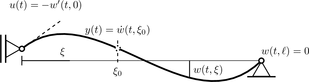
Our objective is to stabilise the system exponentially. This can be achieved by applying velocity feedback at the left endpoint, that is, by using the control law \[u(t)=-k\dot{w}(t,0)\] with \(k>0\). According to [21], this feedback law renders the system exponentially stable. Since only the velocity at the interior point \(\xi_0\) is measured, however, the boundary velocity \(\dot{w}(t,0)\) is not directly available. We therefore apply the framework developed above to reconstruct this quantity from the input and output.

We first represent 35 as a system node. As is customary for the wave equation, we introduce the state \[x(t) = \left( \begin{smallmatrix} q(t)\\ p(t) \end{smallmatrix} \right) \mathrel{\vcenter{:}}= \left( \begin{smallmatrix} w^\prime(t,\cdot)\\ \dot{w}(t,\cdot) \end{smallmatrix} \right) \in L^2([0,\ell];\mathbb{R}^2).\] Here, \(q(t),p(t)\in L^2([0,\ell])\) denote the spatial distributions of the strain and momentum, respectively. In the present dimensionless setting, the momentum coincides with the velocity. Since the clamping condition \(w(t,\ell)=0\) implies \(p(t,\ell)=0\), the system can be written in the form 4 with \(S=\left[\begin{smallmatrix}A\&B\\[-1mm]\\C\&D\end{smallmatrix}\right]\), where \[\label{eq:wavenode} \begin{equation} \begin{align} \operatorname{dom}(S)=\operatorname{dom}(A\&B) &= \left\{ \left( \begin{smallmatrix} q\\ p\\ u \end{smallmatrix} \right) \in H^1([0,\ell];\mathbb{R}^2)\times\mathbb{R} \left\vert\vphantom{ \left( \begin{smallmatrix} q\\ p\\ u \end{smallmatrix} \right) \in H^1([0,\ell];\mathbb{R}^2)\times\mathbb{R} } p(\ell)=0 \;\wedge\; -q(0)=u \right.\right\}, \\ A\&B \left( \begin{smallmatrix} q\\ p\\ u \end{smallmatrix} \right) &= \left( \begin{smallmatrix} p^\prime\\ q^\prime \end{smallmatrix} \right), \qquad C\&D \left( \begin{smallmatrix} q\\ p\\ u \end{smallmatrix} \right) = p(\xi_0). \end{align} \end{equation} The fact that this defines a system node on (L^2([0,\ell];\mathbb{R}^2),\mathbb{R},\mathbb{R}) can be established using the techniques developed in \cite{PhReSc23}. The class considered there differs only in that the output is a boundary value. Replacing this boundary output by the interior point evaluation above does not affect the system-node property. To reconstruct the velocity at the left endpoint, we introduce the additional output \eqref{eq:zout} determined by K\&L\in\operatorname{dom}(A\&B)^\prime with \begin{equation} K\&L \left( \begin{smallmatrix} q\\ p\\ u \end{smallmatrix} \right) = p(0). \end{equation}\tag{36}\]

We next determine the adjoint of the extended system node \[S_{\rm ext} = \left[ \begin{smallmatrix} A\&B\\ C\&D\\ K\&L \end{smallmatrix} \right].\] Let \(\varphi_q,\varphi_p\in L^2([0,\ell])\) and \(\eta,\alpha\in\mathbb{R}\). Then \[\label{eq:waveadj} \begin{align} & \left\langle \left( \begin{smallmatrix} \varphi_q\\ \varphi_p\\ \eta\\ \alpha \end{smallmatrix} \right), \left[ \begin{smallmatrix} A\&B\\ C\&D\\ K\&L \end{smallmatrix} \right] \left( \begin{smallmatrix} q\\ p\\ u \end{smallmatrix} \right) \right\rangle \\ &\qquad = \left\langle \left( \begin{smallmatrix} \varphi_q\\ \varphi_p\\ \eta\\ \alpha \end{smallmatrix} \right), \left( \begin{smallmatrix} p^\prime\\ q^\prime\\ p(\xi_0)\\ p(0) \end{smallmatrix} \right) \right\rangle_{L^2([0,\ell];\mathbb{R}^2)\times\mathbb{R}^2} \\ &\qquad = \int_0^\ell \varphi_q(\xi)p^\prime(\xi) + \varphi_p(\xi)q^\prime(\xi) \,{\rm d}\xi + \eta p(\xi_0) + \alpha p(0). \end{align}\tag{37}\] Assume that \[\left( \begin{smallmatrix} \varphi_q\\ \varphi_p\\ \eta\\ \alpha \end{smallmatrix} \right) \in\operatorname{dom}(S_{\rm ext}^*).\] Choosing \(p,q\in C_0^\infty([0,\ell])\) with \(\xi_0\notin\mathop{\mathrm{supp}}(p)\) and using the definition of the weak derivative gives \[\varphi_p\in H^1([0,\ell]), \qquad \varphi_q|_{[0,\xi_0]}\in H^1([0,\xi_0]), \qquad \varphi_q|_{[\xi_0,\ell]}\in H^1([\xi_0,\ell]). \label{eq:phismooth}\tag{38}\] We denote the left and right limits of a function \(f\) at \(\xi_0\) by \(f(\xi_0^-)\) and \(f(\xi_0^+)\), respectively. Moreover, \(\varphi_q^\prime\in L^2([0,\ell])\) denotes the function that coincides with the weak derivative of \(\varphi_q|_{[0,\xi_0]}\) on \([0,\xi_0]\) and with that of \(\varphi_q|_{[\xi_0,\ell]}\) on \([\xi_0,\ell]\).

Using \(p(\ell)=0\) and \(q(0)=-u\), the right-hand side of 37 becomes \[\begin{align} & -\int_0^{\xi_0} \varphi_q^\prime(\xi)p(\xi)\,{\rm d}\xi + \varphi_qp\Big|_0^{\xi_0^-} - \int_{\xi_0}^\ell \varphi_q^\prime(\xi)p(\xi)\,{\rm d}\xi + \varphi_qp\Big|_{\xi_0^+}^{\ell} \\ &\qquad - \int_0^\ell \varphi_p^\prime(\xi)q(\xi)\,{\rm d}\xi + \varphi_pq\Big|_0^\ell + \eta p(\xi_0) + \alpha p(0) \\ &= -\int_0^\ell \big( \varphi_q^\prime(\xi)p(\xi) + \varphi_p^\prime(\xi)q(\xi) \big) \,{\rm d}\xi \\ &\qquad + \big( \varphi_q(\xi_0^-) - \varphi_q(\xi_0^+) + \eta \big)p(\xi_0) + \big( \alpha-\varphi_q(0) \big)p(0) + \varphi_p(\ell)q(\ell) + \varphi_p(0)u. \end{align}\] Consequently, \[\begin{align} \operatorname{dom}(S_{\rm ext}^*) &= \left\{ \left( \begin{smallmatrix} \varphi_q\\ \varphi_p\\ \eta\\ \alpha \end{smallmatrix} \right) \in L^2([0,\ell];\mathbb{R}^2)\times\mathbb{R}^2 \left\vert\vphantom{ \left( \begin{smallmatrix} \varphi_q\\ \varphi_p\\ \eta\\ \alpha \end{smallmatrix} \right) \in L^2([0,\ell];\mathbb{R}^2)\times\mathbb{R}^2 } \begin{array}{l} \eqref{eq:phismooth}\text{ holds},\; \varphi_p(\ell)=0,\\ \alpha=\varphi_q(0),\; \eta=\varphi_q(\xi_0^+)-\varphi_q(\xi_0^-) \end{array} \right.\right\}, \\ S_{\rm ext}^* \left( \begin{smallmatrix} \varphi_q\\ \varphi_p\\ \eta\\ \alpha \end{smallmatrix} \right) &= \left( \begin{smallmatrix} -\varphi_p^\prime\\ -\varphi_q^\prime\\ \varphi_p(0) \end{smallmatrix} \right). \end{align}\]

Thus, the system governed by \(S_{\rm ext}^*\) is again a wave equation, with a clamped condition at the right endpoint and force control at the left endpoint, together with an interface condition at \(\xi_0\). Define \(\varphi_w:\mathbb{R}_{\geq0}\to H^1([0,\ell])\) by \[\varphi_w(t,\xi) = \int_\xi^\ell \varphi_q(t,\zeta)\,{\rm d}\zeta. \label{eq:wadj}\tag{39}\] The adjoint system can then be written as \[\begin{align} \ddot{\varphi}_w(t,\xi) &=\phantom{-}\varphi_w^{\prime\prime}(t,\xi), && (t,\xi)\in\mathbb{R}_{\geq0}\times \big((0,\xi_0)\cup(\xi_0,\ell)\big), \\ \alpha(t) &=-\varphi_w^\prime(t,0), && t\in\mathbb{R}_{\geq0}, \\ \eta(t) &=-\varphi_w^\prime(t,\xi_0^+) +\varphi_w^\prime(t,\xi_0^-), && t\in\mathbb{R}_{\geq0}, \\ 0 &=\phantom{-}\varphi_w(t,\ell), && t\in\mathbb{R}_{\geq0}, \\ \mu(t) &=\phantom{-}\dot{\varphi}_w(t,0), && t\in\mathbb{R}_{\geq0}. \end{align} \label{eq:waveqadj}\tag{40}\] The input \(\eta\) may therefore be interpreted as a point force acting at \(\xi_0\).

We now construct a generalised null control. Set \(h\mathrel{\vcenter{:}}= \frac{\ell}{q}\), so that \(\xi_0=ph\), \(\ell=qh\). We use the right-shift operator \(S_{r,h}\) introduced in Section 2. Thus, \(S_{r,h}^j\) represents a delay of length \(jh\). In particular, \(S_{r,h}^j\delta=\delta_{jh}\). For a polynomial \(P(X)=p_0+p_1X+\cdots+ p_NX^N\), we use the notation \[P(S_{r,h}) \mathrel{\vcenter{:}}= \sum_{j=0}^N p_jS_{r,h}^j.\] Since \(p\) and \(q\) are coprime and at least one of them is even, the polynomials \(1+X^{2p}\), \(1+X^{2q}\) are coprime. Hence, there exist polynomials \(P,Q\in\mathbb{R}[X]\) satisfying the Bézout identity \[P(X)(1+X^{2p})+Q(X)(1+X^{2q})=1. \label{eq:wavebezout}\tag{41}\] To determine a corresponding null control, introduce the Riemann invariants \[R\mathrel{\vcenter{:}}= \dot{\varphi}_w+\varphi_w^\prime, \qquad S\mathrel{\vcenter{:}}= \dot{\varphi}_w-\varphi_w^\prime.\] On both subintervals \((0,\xi_0)\) and \((\xi_0,\ell)\), they satisfy \[\dot{R}-R^\prime=0, \qquad \dot{S}+S^\prime=0.\] Thus, \(R\) and \(S\) represent left- and right-travelling waves, respectively. Consider a smooth input \(\alpha\in C_0^\infty(\mathbb{R}_{>0})\) and zero initial conditions. At the interface, define \[\begin{align} s_-(t)&\mathrel{\vcenter{:}}= S(t,\xi_0^-), & r_+(t)&\mathrel{\vcenter{:}}= R(t,\xi_0^+), \\ r_-(t)&\mathrel{\vcenter{:}}= R(t,\xi_0^-), & s_+(t)&\mathrel{\vcenter{:}}= S(t,\xi_0^+). \end{align}\] Continuity of \(\dot{\varphi}_w\) and the interface condition in 40 yield \[r_-=r_++\eta, \qquad s_+=s_-+\eta. \label{eq:waveinterface}\tag{42}\] Propagation between the interface and the two endpoints gives \[s_- = S_{r,h}^{2p}r_- + 2S_{r,h}^p\alpha, \qquad r_+ = -S_{r,h}^{2(q-p)}s_+. \label{eq:wavepropagation}\tag{43}\] Indeed, the first identity describes propagation to the left endpoint and back, together with the boundary input \(\alpha\), whereas the second identity incorporates the sign change caused by reflection at the clamped endpoint. Combining 42 and 43 , we obtain \[\big(I+S_{r,h}^{2q}\big)s_+ = 2S_{r,h}^p\alpha + \big(I+S_{r,h}^{2p}\big)\eta. \label{eq:wavecharrelation}\tag{44}\] Motivated by the Bézout identity 41 , define \[\eta_\alpha \mathrel{\vcenter{:}}= -2P(S_{r,h})S_{r,h}^p\alpha. \label{eq:waveadjinp}\tag{45}\] Then 44 and 41 give \[\big(I+S_{r,h}^{2q}\big)s_+ = 2\big(I+S_{r,h}^{2q}\big) Q(S_{r,h})S_{r,h}^p\alpha.\] Since \(I+S_{r,h}^{2q}\) is injective on causal distributions, it follows that \[s_+ = 2Q(S_{r,h})S_{r,h}^p\alpha.\] The remaining travelling-wave components are therefore \[\begin{align} r_+ &= -2S_{r,h}^{2q-p}Q(S_{r,h})\alpha, \\ r_- &= -2S_{r,h}^p \big( P(S_{r,h}) + S_{r,h}^{2(q-p)}Q(S_{r,h}) \big)\alpha, \\ s_- &= 2S_{r,h}^p \big( P(S_{r,h})+Q(S_{r,h}) \big)\alpha. \end{align}\] Consequently, all travelling-wave components are finite linear combinations of delayed copies of \(\alpha\). In particular, the corresponding adjoint state has compact temporal support.

At the left endpoint, \[\alpha=\tfrac{1}{2}(S-R), \qquad \mu=\tfrac{1}{2}(S+R),\] and the incoming left-travelling wave is given by \(S_{r,h}^p r_-\). Hence, \[\mu_\alpha = \alpha+S_{r,h}^p r_-.\] Using 41 , we obtain \[\mu_\alpha = A(S_{r,h})\alpha, \qquad A(X) \mathrel{\vcenter{:}}= P(X)(1-X^{2p})+Q(X)(1-X^{2q}). \label{eq:waveadjout}\tag{46}\] Equivalently, \[A(X) = 1-2X^{2p}P(X)-2X^{2q}Q(X).\]

Let \((\alpha_n)\) be a one-sided mollifier sequence satisfying \[\mathop{\mathrm{supp}}\alpha_n\subset(0,h/n], \qquad \alpha_n\longrightarrow\delta \quad\text{in }H^{-1}_{0,\mathrm{loc}}(\mathbb{R}_{\geq0}).\] Define \(\eta_n \mathrel{\vcenter{:}}= -2P(S_{r,h})S_{r,h}^p\alpha_n\), \(\mu_n \mathrel{\vcenter{:}}= A(S_{r,h})\alpha_n\), and let \(\varphi_n\) be the corresponding adjoint state. Since all travelling-wave components consist of finitely many fixed delays of \(\alpha_n\), there exists some \(T>0\), independent of \(n\), such that \[\mathop{\mathrm{supp}}\varphi_n\subset[0,T], \qquad \mathop{\mathrm{supp}}\eta_n\subset[0,T], \qquad \mathop{\mathrm{supp}}\mu_n\subset[0,T].\] Passing to the distributional limit gives \[\eta = -2P(S_{r,h})S_{r,h}^p\delta, \qquad \mu = A(S_{r,h})\delta,\] together with a corresponding adjoint state \(\varphi\) satisfying \(\mathop{\mathrm{supp}}\varphi\subset[0,T]\). Thus, \(\eta\) is a generalised null control satisfying the assumptions of Theorem 7, for instance with \(k=1\). Consequently, for every generalised trajectory of 35 , understood as a trajectory of the system node 36 , the distribution \(u\ast\mu-y\ast\eta\) coincides on \((T,\infty)\) with the velocity at the left endpoint. Therefore, \[\dot{w}(\cdot,0) = A(S_{r,h})u + 2P(S_{r,h})S_{r,h}^p y \qquad \text{on }(T,\infty). \label{eq:wavevelocityreconstruction}\tag{47}\] The Bézout identity 41 evaluated at \(X=0\) gives \[P(0)+Q(0)=1,\] and hence \(A(0)=1\). We may therefore write \[A(X)=1+\widetilde{A}(X), \qquad \widetilde{A}(0)=0.\] The exponentially stabilising feedback law \[u(t)=-k\dot{w}(t,0), \qquad k>0,\] can thus be realised, after time \(T\), in the causal form \[u = -\frac{k}{1+k} \left( \widetilde{A}(S_{r,h})u + 2P(S_{r,h})S_{r,h}^p y \right). \label{eq:wavefeedbackrealisation}\tag{48}\] Since \(\widetilde{A}(0)=0\) and \(p\geq1\), the right-hand side of 48 contains only delayed values of the input and output.

For example, if \(\xi_0=\ell/2\), then \(p=1\) and \(q=2\). One possible choice in 41 is \(P(X)=\tfrac12-\tfrac12 X^2\), \(Q(X)=\tfrac{1}{2}\). In this case, \(\eta=-\delta_h+\delta_{3h}\), \(\mu=\delta-\delta_{2h}\). The corresponding adjoint state is supported in \([0,3h]\). Hence, Theorem 7 applies with \(T=3h=\tfrac{3\ell}{2}\), and 47 becomes \[\dot{w}(t,0) = u(t)-u(t-2h)+y(t-h)-y(t-3h), \qquad t>3h.\] Consequently, the stabilising feedback law \(u(t)=-k\dot{w}(t,0)\) can be implemented as \[u(t) = \frac{k}{1+k} \left( u(t-\ell) -y\left(t-\tfrac{\ell}{2}\right) +y\left(t-\tfrac{3\ell}{2}\right) \right), \qquad t>\tfrac{3\ell}{2}.\]

7.2 State reconstruction for a reaction–diffusion equation with Dirichlet boundary control↩︎

Consider a reaction–diffusion equation on the rectangular domain \(\Omega=(0,L_1)\times(0,L_2)\subset\mathbb{R}^2\). The control acts through the Dirichlet boundary values on the right-hand part of the boundary, \[\Gamma=\{L_1\}\times[0,L_2]\subset\partial\Omega,\] while homogeneous Dirichlet boundary conditions are imposed on \(\partial\Omega\setminus\Gamma\). The output is given by the negative Neumann trace on \(\Gamma\). We consider a unit diffusion coefficient and a spatially constant reaction coefficient \(c\in\mathbb{R}\). Thus, the system is governed by \[\label{eq:rdeq} \begin{align} \dot{x}(t,\xi) &=\phantom{-} \Delta x(t,\xi)+cx(t,\xi), &(t,\xi)&\in\mathbb{R}_{\geq0}\times\Omega, \\ u(t,\xi) &=\phantom{-} x(t,\xi), &(t,\xi)&\in\mathbb{R}_{\geq0}\times\Gamma, \\ 0 &=\phantom{-} x(t,\xi), &(t,\xi)&\in\mathbb{R}_{\geq0}\times \big(\partial\Omega\setminus\Gamma\big), \\ y(t,\xi) &=- n^\top(\xi)\nabla x(t,\xi), &(t,\xi)&\in\mathbb{R}_{\geq0}\times\Gamma, \end{align}\tag{49}\] where \(n\in L^\infty(\partial\Omega;\mathbb{R}^2)\) denotes the outward unit normal vector field on \(\partial\Omega\).

We next formulate 49 as a system node. The state space is \(L^2(\Omega)\). Since the full Dirichlet trace belongs to the fractional Sobolev space \(H^{1/2}(\partial\Omega)\); see [3], the input space is chosen as \(H^{1/2}_0(\Gamma)\). This is the space of all elements of \(H^{1/2}(\Gamma)\) whose extension by zero to \(\partial\Omega\setminus\Gamma\) belongs to \(H^{1/2}(\partial\Omega)\); see also [2]. The output space is \[H^{-1/2}(\Gamma)\mathrel{\vcenter{:}}= H^{1/2}_0(\Gamma)^\prime.\] Let \(\gamma:H^1(\Omega)\to H^{1/2}(\partial\Omega)\) denote the trace operator, and define \[H^1_\Gamma(\Omega) = \left\{ x\in H^1(\Omega) \left\vert\vphantom{x\in H^1(\Omega)} (\gamma x)|_{\partial\Omega\setminus\Gamma}=0 \right.\right\}.\] The restricted trace operator \[\gamma_\Gamma:H^1_\Gamma(\Omega)\to H^{1/2}_0(\Gamma)\] maps a function to the restriction of its trace to \(\Gamma\). Furthermore, let \(H_{\operatorname{div}}(\Omega)\) denote the space of all vector fields in \(L^2(\Omega;\mathbb{R}^2)\) whose weak divergence belongs to \(L^2(\Omega)\). The restricted normal trace operator is denoted by \[\gamma_{\Gamma,n}:H_{\operatorname{div}}(\Omega)\to H^{-1/2}(\Gamma);\] see [2]. For the basic properties of the normal trace operator, we refer to [22].

With these spaces and trace operators, the system node associated with 49 is given by \[\label{eq:rdeqnode} \begin{align} \operatorname{dom}S=\operatorname{dom}(A\&B) &= \left\{ \left(\begin{smallmatrix}x\\u\end{smallmatrix}\right)\in H^1_\Gamma(\Omega)\times H^{1/2}_0(\Gamma) \left\vert\vphantom{ \left(\begin{smallmatrix}x\\u\end{smallmatrix}\right)\in H^1_\Gamma(\Omega)\times H^{1/2}_0(\Gamma) } \nabla x\in H_{\operatorname{div}}(\Omega) \;\wedge\; u=\gamma_\Gamma x \right.\right\}, \\ A\&B\left(\begin{smallmatrix}x\\u\end{smallmatrix}\right) &= \Delta x+cx, \qquad C\&D\left(\begin{smallmatrix}x\\u\end{smallmatrix}\right) =- \gamma_{\Gamma,n}(\nabla x). \end{align}\tag{50}\] A direct calculation shows that \(S\) is a self-dual system node, that is, \(S=S^\prime\). Consequently, if \[\mathcal{R}:H^{1/2}_0(\Gamma)\to H^{-1/2}(\Gamma)\] denotes the Riesz isomorphism, then the adjoint of \(S\) satisfies \[S^* = \left[\begin{smallmatrix}I & 0\\0 & \mathcal{R}^{-1}\end{smallmatrix}\right] S \left[\begin{smallmatrix}I & 0\\0 & \mathcal{R}^{-1}\end{smallmatrix}\right]. \label{eq:rdadj}\tag{51}\]

We now apply the state-reconstruction procedure developed in Section 5. To this end, we determine null controls for the adjoint system. By 51 , the adjoint differs from the original system 49 only through the Riesz identifications of its input and output spaces. More precisely, the adjoint system is described by \[\label{eq:rdeq95adj} \begin{align} \dot{\varphi}(t,\xi) &=\phantom{-} \Delta\varphi(t,\xi)+c\varphi(t,\xi), &(t,\xi)&\in\mathbb{R}_{\geq0}\times\Omega, \\ \widetilde{\eta}(t,\xi) &=\phantom{-} \varphi(t,\xi), &(t,\xi)&\in\mathbb{R}_{\geq0}\times\Gamma, \\ 0 &=\phantom{-} \varphi(t,\xi), &(t,\xi)&\in\mathbb{R}_{\geq0}\times \big(\partial\Omega\setminus\Gamma\big), \\ \widetilde{\mu}(t,\xi) &= -n^\top(\xi)\nabla\varphi(t,\xi), &(t,\xi)&\in\mathbb{R}_{\geq0}\times\Gamma. \end{align}\tag{52}\] The abstract input and output of the adjoint system are related to these traces by \[\label{eq:rcriesz} \eta(\cdot,t) = \mathcal{R}\widetilde{\eta}(\cdot,t), \qquad \mu(\cdot,t) = \mathcal{R}^{-1}\widetilde{\mu}(\cdot,t), \qquad t\in\mathbb{R}_{\geq0}.\tag{53}\] The results of [23], [24] imply that, for every \(T>0\) and \(\varphi_0\in L^2(\Omega)\), there exists a null control \[\widetilde{\eta} \in L^2([0,T];H^{1/2}_0(\Gamma))\] such that the solution of 52 satisfying \(\varphi(0,\cdot)=\varphi_0\) fulfils \(\varphi(T,\cdot)=0\). The corresponding output satisfies \[\widetilde{\mu} \in L^2([0,T];H^{-1/2}(\Gamma)).\] Consequently, \[\eta\in L^2([0,T];H^{-1/2}(\Gamma)), \qquad \mu\in L^2([0,T];H^{1/2}_0(\Gamma)).\] Thus, in this case, the reconstruction can be formulated entirely in terms of functions rather than distributions.

The results of Section 5 then imply that every generalised, and hence every classical, trajectory of 49 satisfies \[\forall\,t\geq T:\quad \langle x(t),\varphi_0\rangle_{L^2} = \int_0^T \langle u(t-\tau),\mu(\tau)\rangle_{H^{1/2}} - \langle y(t-\tau),\eta(\tau)\rangle_{H^{-1/2}} \,{\rm d}\tau. \label{eq:concrd}\tag{54}\]

The Riesz isomorphism can be eliminated from the final reconstruction formula. Indeed, its definition gives \[\forall\,v\in H^{-1/2}(\Gamma),\; w\in H^{1/2}_0(\Gamma):\quad \langle v,\mathcal{R}w\rangle_{H^{-1/2}} = \langle v,w\rangle_{H^{-1/2},H^{1/2}} = \langle\mathcal{R}^{-1}v,w\rangle_{H^{1/2}}.\] Hence, 54 is equivalent to \[\forall\,t\geq T:\quad \langle x(t),\varphi_0\rangle_{L^2} = \int_0^T \langle u(t-\tau),\widetilde{\mu}(\tau)\rangle_{H^{1/2},H^{-1/2}} - \langle y(t-\tau),\widetilde{\eta}(\tau)\rangle_{H^{-1/2},H^{1/2}} \,{\rm d}\tau.\] Thus, the two terms in the integrand are duality pairings between the Dirichlet and Neumann traces of the original and adjoint systems.

For the numerical illustration, we compute null controls for the adjoint system 52 and reconstruct the projection of the state using 31 , with the inner products in that formula replaced by the corresponding duality pairings. The orthonormal family \((\varphi_{0j})_{j\in\mathbb{N}}\) is obtained by applying the Gram–Schmidt procedure to a basis of bivariate polynomials of total degree at most ten. This results in an approximation space of dimension \(N=66\). The simulation results are shown in Fig. 2.

Conclusion↩︎

We have developed a modulating-function framework for partial state reconstruction from past input and output data. The approach is based on generalised null controls of the adjoint system and corresponding convolutions with the input and output.

The first main contribution is a unified formulation for infinite-dimensional linear systems in the system-node framework. This framework requires comparatively few assumptions, is closed under adjunction, and does not require the system to be well-posed. The second contribution is a distributional extension of the modulating-function method. The resulting modulating distributions allow the reconstruction of additional outputs defined by unbounded operators and are therefore particularly suitable for the implementation of unbounded state feedback.

The theoretical results were illustrated by two examples. For a vibrating string, the distributional approach was used to reconstruct a boundary velocity from input and output data and thereby realise an exponentially stabilising feedback law. For a reaction–diffusion equation with Dirichlet boundary control and Neumann boundary observation, the method was applied to finite-dimensional state reconstruction and illustrated numerically.

References↩︎