Capital Asset Pricing Model with Size Factor and Normalizing by Volatility Index
November 29, 2024
Abstract
The Capital Asset Pricing Model (CAPM) relates a well-diversified stock portfolio to a benchmark portfolio. We insert size effect in CAPM, capturing the observation that small stocks have higher risk and return than large stocks, on average. For some size-based stock portfolios, dividing their returns by the Volatility Index makes them closer to independent and normal. In this article, we combine these ideas to create a new discrete-time model, which includes volatility, relative size, and CAPM. We fit this model using real-world data, prove the long-term stability, and connect this research to Stochastic Portfolio Theory. We fill important gaps in our previous article on CAPM with the size factor.
1 Introduction↩︎
Here, we briefly describe the parts of the model analyzed in this article. We remind the readers that price returns for a stock or a portfolio measure only price changes, ignoring dividends, while total returns include both price changes and dividends paid. Also, equity premium is computed as total returns minus risk-free returns (usually measured by short-term Treasury bills). We combine three main ideas in this article.
Idea 1: Capital Asset Pricing Model. We model a target stock portfolio (well-diversified) using a simple linear regression versus the benchmark stock portfolio. A typical example is the Standard & Poor 500 (S&P 500), a well-known index of large USA stocks. The classic measuring tool there is equity premia (for target and benchmark), but we can also apply this for price returns. The slope and intercept of this regression are called beta and alpha.
Idea 2: Size Effect. Small stocks, on average, have higher volatility but also higher returns than large stocks, see the classic articles [1], [2]. This feature implies long-term stability: Well-diversified stock portfolios stay together and not split into several clouds. We combined these two ideas in the previous article by the second author [3]. This article is a sequel of that work. Such long-term stability is of interest in Stochastic Portfolio Theory, which constructs portfolios as functions of market weights, utilizing the observation that small stocks have higher risk and return.
Idea 3: The Volatility Index. In another article [4] by the second author, we observe that total monthly returns of the benchmark are not IID (independent identically distributed) Gaussian. However, dividing them by volatility makes them IID Gaussian. Here, volatility is measured by the Volatility Index (VIX) monthly average. The volatility itself is modeled as an autoregression of order 1 on the logarithmic scale. Similar observation holds for price monthly returns of large stocks, and for the small stocks.
In this article, we continue research of [3] by inserting Idea 3 in this setting, thus combining all three ideas. We create a new discrete-time model, and fit it using real market data from Kenneth French’s data library and Federal Reserve Economic Data web site. We then state and prove long-term stability of this market model, and interpret this for Stochastic Portfolio Theory. Unlike [3], we consider only discrete time models in this article. We fill a couple of important gaps left in the previous research [3].
In Section 2, we provide a comprehensive motivation of proposed models and a literature review. As a motivation to use the volatility to normalize the returns and premia, we do a simple graphical analysis of real-world
financial data. Section 3 is devoted to real-world financial data description, and statistical fit of these models. In Section 4, we state and prove long-term stability (ergodicity) result for
this model: Theorem 1. It does not contain any simulations or empirical data analysis. In Section 5, we interpret our
results in terms of Stochastic Portfolio Theory. We simulate capital distribution curve (ranked market weights vs ranks). We state and prove a rigorous long-term stability result for this curve in Theorem 2. Next, Theorem 3 contains results about its shape:
We reduce it to normal order statistics. Finally, the Appendix contains a discussion of the capital distribution curve based on ranked standard normal sample, continuing the research of Section 5, and doing some more theorems with proofs and simulations. All data and code are available on GitHub repository asarantsev/size-capm-vix
2 Background and Motivation↩︎
2.1 Capital Asset Pricing Model↩︎
This celebrated model, abbreviated as CAPM, compares returns of a stock portfolio with returns of the benchmark. This model was proposed by [5]–[7]. The benchmark is usually taken to be the Standard & Poor 500 for the American stock market. The model states that the only factor which matters for a well-diversified portfolio is market exposure, otherwise known by a standard term beta and denoted by \(\beta\). The case \(\beta = 0\) corresponds to the risk-free portfolio, with guaranteed deterministic return. This is usually measured using a benchmark of a short-term rate \(r\), for example 1-month Treasury rate. The case \(\beta = 1\) corresponds to the market portfolio (the benchmark). When \(\beta \in (0, 1)\), the stock portfolio can be replicated by investing in a portfolio of risk-free bonds and the stock market benchmark, in proportions \(1 - \beta\) and \(\beta\), respectively. In other words, total returns \(Q\) (including price changes and dividends) of this portfolio are related to total returns \(Q_0\) of the benchmark: \[\label{eq:CAPM-Q} Q = (1-\beta)r + \beta Q_0.\tag{1}\] Equivalently, we can rewrite 1 in terms of equity premia \(P = Q - r\) of the portfolio and \(P_0 = Q_0 - r\) of the benchmark: \[\label{eq:CAPM} P = \beta P_0.\tag{2}\] If \(\beta > 1\), this 2 still holds, and can be interpreted as shorting bonds and investing everything in the benchmark. We can treat \(\beta\) as a risk measure: \(\beta > 1\) means that the portfolio is riskier than the benchmark, and \(\beta \in (0, 1)\) means the opposite. The case \(\beta < 0\) does not usually happen in practice, see [8].
It is not considered a big achievement if a money manager improved returns by increasing \(\beta\). In fact, often these managers are expected to maximize excess return: Total returns of a portfolio adjusted for market exposure. This quantity is denoted by \(\alpha\) and, accordingly, is called alpha. These two Greek letters \(\alpha\) and \(\beta\) are standard notation in Finance. This methodology of market exposure and excess return is well-accepted by both finance academics and practitioners. One can include \(\alpha\) into 2 as \[\label{eq:alpha-beta} P = \alpha + \beta P_0 + \varepsilon,\quad \mathbb{E}\varepsilon = 0.\tag{3}\] We also include an error term \(\varepsilon\), since the model might not hold almost surely. This makes 3 a simple linear regression of \(P\) upon \(P_0\).
Subsequent research disproved the strong claims of CAPM that market exposure \(\beta\) is the only risk measure and quantity of interest for a diversified stock portfolio, see [2], [9], and [8]. For one, there are systematic ways to generate excess return \(\alpha\) by using several factors. Also, \(\beta\) might be unstable in the long run. Still, \(\beta\) is an established risk measure, accepted by financial theorists, analysts, and managers. The CAPM is useful as a benchmark model, a starting point for more complicated and real-life models. Calculating \(\beta\) for mutual funds and exchange-traded funds is common practice.
2.2 Size and value↩︎
The most well-known and accepted factors are size (average market capitalization of portfolio stocks) and value (fundamentals such as earnings, dividends, or book value, compared to price). These are well-accepted by financial academic community and are considered useful by industry practitioners, to the extent that there are multiple size- and value-based funds traded alongside the S&P 500 funds. See [1], [2], [10].
Including a few factors (for example size and value) would enrich 3 . In particular, size factor is related to \(\beta\) as follows: Well-diversified portfolios of small stocks have equity premia \(P\) closely correlated with that \(P_0\) of large stock benchmark S&P 500. This simple linear regression of \(P\) vs \(P_0\) has very large \(R^2\) but \(\beta\) which is slightly larger as \(1\). This can be done, for example, with exchange-traded funds tracking small, mid, and large (=benchmark) stock indices, see [3]. The \(\beta\) for mid-cap index is 1.15, and for small-cap index is 1.27. A natural idea then is to model the \(\beta\) as a function of a portfolio size relative to benchmark.
Additionally, we could model the \(\alpha\) similarly, as a function of a portfolio size relative to benchmark. However, this might not be as important as for the \(\beta\). Indeed, in [3] we have \(\alpha\) is not significantly different from zero for both small-cap and mid-cap indices. See more on the size effect in [11], and the discussion in [8].
2.3 CAPM-based model with size as factor↩︎
Therefore, we developed the following model in [3]: Let \(S\) = market capitalization of target portfolio, and \(S_0\) = market capitalization of benchmark portfolio. Then the relative size (on the log scale) is defined as \[\label{eq:relsize} C = \ln(S_0/S)\tag{4}\] For \(C = 0\), the relative size is 0 (on the log scale) or 1 (on the absolute scale). This corresponds to the target portfolio having the same properties as the benchmark portfolio, with \(\alpha = 0\) and \(\beta = 1\). The simplest model is linear: For some coefficients \(a, b\), \[\label{eq:alpha-beta-functions} \alpha = aC, \quad \beta = bC + 1\tag{5}\] In fact, in [3] we have more general conditions: \(\alpha\) and \(\beta\) are general functions of \(C\). Here, we focus only on linear functions, see [3]. Analysis for small-cap and mid-cap funds above shows that \(a \approx 0\) but \(b > 0\). Rewrite 3 as follows by plugging there 5 : \[\label{eq:CAPM-size} P = AC + \left(1 + BC\right)P_0 + \delta,\tag{6}\] where \(\delta\) are IID regression residuals with mean zero. A good way to generalize 6 is to make it dynamic: a time series. To this end, we make the model complete by writing an equation for \(S, S_0, P_0\). With regard to the benchmark equity premia \(P_0\) and market cap \(S_0\), we shall write this equation in the next subsection. Unlike total returns, which include dividends, price returns are computed only using price movements. The main idea is to take CAPM linear regression, and replace equity premia with price returns. We get \[\label{eq:returns-size} R = aC + \left(1 + bC\right)R_0 + \varepsilon,\tag{7}\] where \(a, b\) are some coefficients (not necessarily the same as the \(A, B\) from 6 ), and \(\varepsilon\) are IID regression residuals with mean zero (not necessarily the same as \(\varepsilon\), but possibly correlated with these). We can interpret change in logarithm as price returns: \[\begin{align} \label{eq:d-ln} \begin{aligned} R(t) &= \ln S(t+1) - \ln S(t) = \ln\frac{S(t+1)}{S(t)},\\ R_0(t) &= \ln S_0(t+1) - \ln S_0(t) = \ln\frac{S_0(t+1)}{S_0(t)}. \end{aligned} \end{align}\tag{8}\] In real-life finance, a stock market is stable in the long run: Small stocks grow, on average, faster than large stocks. Thus formerly small stocks might become large, and formerly large stocks might become small. The relative size of a stock portfolio exhibits mean-reversion. In our article [3], we proved this for continuous time and more general systems than 6 , 7 , under the assumptions that the benchmark follows a lognormal Samuelson (Black-Scholes) model of geometric random walk with growth rate \(g\) and total returns \(G\), and \[\label{eq:stability} a + bg < 0.\tag{9}\] This is consistent with the observation made above that \(a \approx 0\) and \(b < 0\), since \(g > 0\). Analysis of real-world finance data in [3] showed that \(A \approx a\) and \(B \approx b\).
2.4 Stochastic volatility↩︎
However, there is a drawback in our modeling from [3]. We fit regressions 6 and 7
using real-world monthly data taken from Kenneth French’s Dartmouth College Financial Data Library. Residuals \(\varepsilon, \delta\) are not IID. Absolute values are autocorrelated. This feature is also true for S&P
500 monthly returns themselves, see our recent article [4]. Also, these returns are not Gaussian. We wish to improve the fit of regressions 6 and 7 to make residuals closer to IID Gaussian. For S&P 500 returns, we did this in [4] as
follows: We divided these returns by monthly average VIX: The S&P 500 Volatility Index \(V\) computed daily by the Chicago Board of Options Exchange. Our main idea of this article [4] is (in our notation, see [4]): \[\label{eq:norm-return}
\frac{R_0(t)}{V(t)} \sim IID Gaussian.\tag{10}\] Similarly, it is reasonable to model normalized equity premia as IID Gaussian: \[\label{eq:norm-premia}
\frac{P_0(t)}{V(t)} \sim IID Gaussian.\tag{11}\] We did not do this in [4], but we complete this work in this article. For the original equity premia
of benchmark \(P_0\), we plot in Figure 1 the quantile-quantile plot and the autocorrelation function for \(P_0\) and \(|P_0|\). For the normalized equity premia \(P_0/V\), we plot these in Figure 2. We see that division by VIX is needed to model
equity premia as in 11 . Data for \(P_0\) is taken from Kenneth French’s data library: Top 10% decile, January 1986–December 2025 (exactly 40 years and 480 months). For short-term rate \(r\), we use the 3-month Treasury rate from Federal Reserve Economic Data: start of month data. Data and Python code is available on Github repository: asarantsev/capm-size-vix
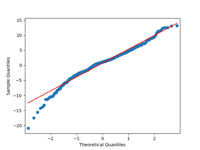
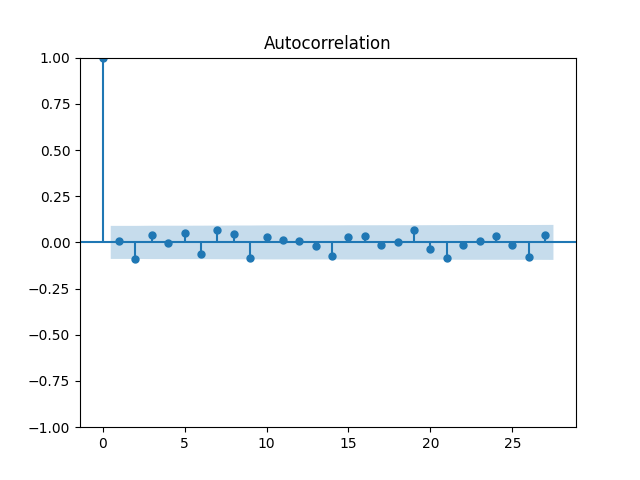
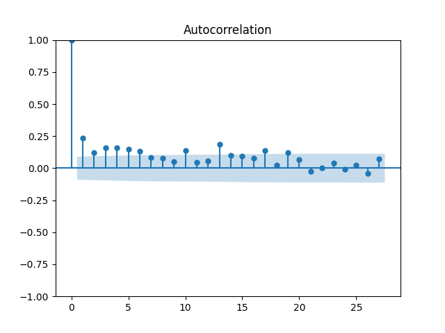
Figure 1: Empirical real-world data: The quantile-quantile (QQ) plot for equity premia \(P_0\), and the empirical autocorrelation function (ACF) for \(P_0\) and for \(|P_0|\), given the monthly data 1986–2025 for equal-weighted portfolio of the top decile \(P_0\)..
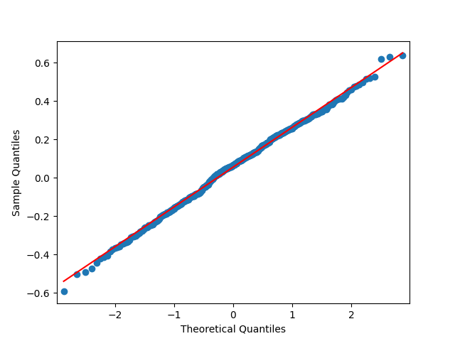
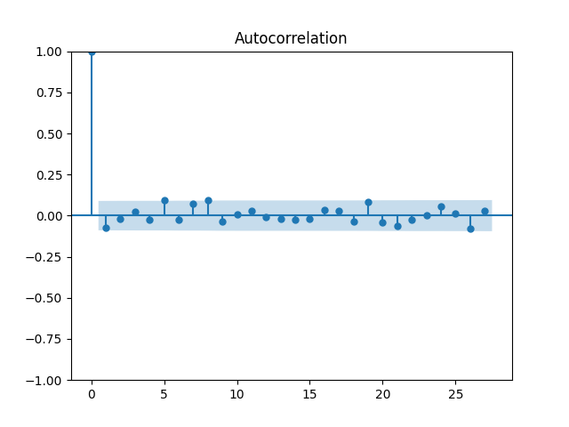
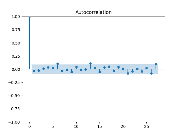
Figure 2: Empirical real-world data: The quantile-quantile (QQ) plot for equity premia \(P_0/V\), and the empirical autocorrelation function (ACF) for \(P_0/V\) and for \(|P_0/V|\), given the monthly data 1986–2025 equal-weighted portfolio of the top decile \(P_0\), normalized by monthly VIX \(V\)..
The VIX itself is modeled by an autoregression of order 1 on the log scale, see [4]: \[\label{eq:ln-VIX} \ln V(t) = \alpha + \beta \ln V(t-1) + W(t).\tag{12}\] Slightly abusing the notation, but following [4], in the rest of the article we use \(\alpha\) and \(\beta\) as the intercept and the slope of this autoregression 12 , instead of excess return and market exposure from the CAPM. This model 12 has good fit, as shown in [4]. Innovations \(W\) are IID but not Gaussian, with some finite exponential moments. The point estimate \(\hat{\beta} = 0.88\), and we reject the unit root hypothesis \(\beta = 1\).
Methodology of [4] stands in contrast to classic stochastic volatility models [12], where the volatility \(V\) is not observed directly and must be inferred from the data \(R_0\) or \(P_0\).
2.5 Capital distribution curve↩︎
A newly developed framework for portfolio management in Stochastic Portfolio Theory, see [13]. One question which concerns it is model stability: In a model of \(N\) stocks, do they move together in the long run, or do they split into several subsets, moving away from each other in the long run? A related question is analysis of market weights: A market weight \(\mu\) of a stock is its market capitalization (size) divided by the sum of all market capitalizations. Rank market weights at each time from top to bottom: \[\mu_{(1)}(t) \ge \ldots \ge \mu_{(N)}(t).\] The plot of \(N\) points \[(\ln n, \ln\mu_{(n)}(t)),\, n = 1, \ldots, N\] is called the capital distribution curve. For real-world markets, this curve is concave and straight at left upper end. See the picture in [13] for 1929, 1939, …, 1999. If the model is stable, the capital distribution curve is also stable in the long run: see Theorem 2. Previous research analyzed long-term stability and capital distribution curve for various continuous-time models: [14], [15]. These models were designed to capture the observations that, on average, small stocks have higher volatility and growth rates than large stocks. In [14], competing Brownian particle models were analyzed, where drift and diffusion coefficients depend on the rank of the stock, and linearity of the capital distribution curve was reproduced. In [15], the drift and diffusion depend on the market weight of a stock, but the capital distribution curve is not linear. These models do not use CAPM or VIX.
In the previous article by the second coauthor [3], devoted to the CAPM with size but without VIX (in other words, with constant volatility), we also reproduced model stability for its continuous-time version [3]. Using simulation, we reproduced the linearity of the capital distribution curve. But we did not state and prove rigorous results on this. A natural question is to reproduce these results for our model here. We accomplish both tasks in this article: (a) we simulate the capital distribution curve in Subsection 5.2, which reproduces its linearity; (b) we prove results on convergence to a Poisson point process. This fills a gap in [3].
2.6 Our contributions↩︎
In this article, we combine the ideas of our articles [3] on CAPM and [4] on VIX to state a reasonable generalization of [3]. This model can be truncated: Include only price changes for the benchmark \(R_0\) and the target \(R\) (or, equivalently, market size \(S_0\) and \(S\)), and volatility \(V\). Alternatively, it can be completed: Include also equity premia \(P_0, P\) for the benchmark and the target. A truncated model contains 3 time series, and a completed model contains 5 time series.
In [3], we model 7 and 6 but with \(P_0\) or \(S_0\) IID Gaussian, in continuous time. The article [3] does not include VIX \(V\). However, this article is concerned with the idea from [4] that division by VIX normalized returns and premia. We replace \(P\) and \(P_0\) with \(P/V\) and \(P_0/V\) in 6 . Also, we replace \(R\) with \(R/V\) and \(R_0\) with \(R_0/V\) in 7 . We model \((R_0/V, P_0/V)\) as IID (but maybe not Gaussian), following 10 and 11 . As mentioned in the Introduction, in Section 3 we perform statistical data analysis.
We fill two lacunas left in our research [3]. The first lacuna is stability results for discrete time. In Section 4 of this article, we state and prove this for the case of stochastic volatility. The second lacuna is rigorous results for the capital distribution curve, which are lacking in [3]. In Section 5 of this article, we state and prove a convergence result for the capital distribution curve: Theorem 2. Next, in Theorem 3, we show a remarkable result: the curve is \[(\ln n, X_{(n)}),\quad n = 1, \ldots, N,\] where \(X_{(1)} \ge \ldots \ge X_{(N)}\) are order statistics of a conditional normal sample: \[X_1, \ldots, X_N \mid \mu, \sigma \sim \mathcal{N}(\mu, \sigma^2)\] for random \(\mu\) and \(\sigma\). We perform the simulation in Section 5 for stochastic VIX. In Appendix, we further analyze this curve for the standard normal \(X_1, \ldots, X_N\), and show its upper left and lower right ends replicate real-world behavior.
3 Financial Data and Statistical Analysis↩︎
3.1 Data description↩︎
We take monthly data January 1986–December 2025. This gives us exactly 40 years and 480 data points. As discussed in the Introduction and Background sections, we measure volatility \(V\) as Chicago Board of Options Exchange VIX: The Volatility Index for S&P 500, monthly average data. This data is taken from Federal Reserve Economic Data (FRED) web site. For equity premia computation, we need short-term Treasury rates, which are also taken from the FRED web site.
The rest of the data is taken from Kenneth French’s Dartmouth College Financial Data Library. It contains equally-weighted portfolios of stocks split into 10 deciles by size: Decile 1 has smallest 10% stocks by size (market capitalization), Decile 2 has
the next 10% smallest stocks, etc up to Decile 10, which contains top 10% largest stocks. We use Decile 10 as the benchmark. We stress that this equally-weighted portfolio of Decile 10 is different from the classic benchmark S&P 500. These portfolios
are reconstituted at the end of June of each year. For each decile and each month, the data contains average market size, price returns (excluding dividends), and total returns (including dividends). The data are available on the GitHub
repository asarantsev/size-capm-vix in the file data-new.xlsx
3.2 Regression description↩︎
Our goal is to fit 7 and 6 . We rewrite these as \[\frac{R(t) - R_0(t)}{V(t)} = aC(t) + bC(t)\frac{R_0(t)}{V(t)} + \varepsilon(t).\] \[\frac{P(t) - P_0(t)}{V(t)} = AC(t) + BC(t)\frac{P_0(t)}{V(t)} + \delta(t).\] These linear regressions do not have an intercept, however. To make the models complete, we add intercepts:
\[\label{eq:returns-reg}
\frac{R(t) - R_0(t)}{V(t)} = aC(t) + bC(t)\frac{R_0(t)}{V(t)} + m + \varepsilon(t).\tag{13}\] \[\label{eq:premia-reg}
\frac{P(t) - P_0(t)}{V(t)} = AC(t) + BC(t)\frac{P_0(t)}{V(t)} + M + \delta(t).\tag{14}\] For the benchmark with price returns \(R_0\) and equity premia \(P_0\), we take Decile
10. For the target with price returns \(R\) and equity premia \(P\), we use Deciles 1, …, 9. Each decile is fit separately. See results in Table 1 and Table 2. The Python code is available on the GitHub repository asarantsev/size-capm-vix in the file
regression-fit.py
| Decile | \(m\) | \(T_{m}\) | \(a\) | \(T_a\) | \(b\) | \(T_b\) | \(s\) |
|---|---|---|---|---|---|---|---|
| 1 | -.12 | -0.64 | .021 | 0.75 | -.025 | -3 | .25 |
| 2 | -.37 | -2.57 | .072 | 2.57 | .012 | 1.3 | .22 |
| 3 | -.21 | -1.64 | .047 | 1.68 | .020 | 2.16 | .19 |
| 4 | -.25 | -2.08 | .06 | 2.09 | .02 | 2.17 | .18 |
| 5 | -.17 | -1.77 | .046 | 1.78 | .033 | 3.56 | .16 |
| 6 | -.027 | -.41 | .009 | .46 | .025 | 2.92 | .13 |
| 7 | -.086 | -1.78 | .032 | 1.88 | .027 | 3.2 | .11 |
| 8 | -.055 | -1.48 | .025 | 1.54 | .03 | 3.46 | .09 |
| 9 | -.02 | -.82 | .015 | .93 | .01 | 1.11 | .07 |
| Decile | \(M\) | \(T_M\) | \(A\) | \(T_A\) | \(B\) | \(T_B\) | \(s\) |
|---|---|---|---|---|---|---|---|
| 1 | -.15 | -.78 | .024 | .85 | -.025 | -3.1 | .25 |
| 2 | -.4 | -2.8 | .077 | 2.75 | .012 | 1.3 | .22 |
| 3 | -.24 | -1.86 | .053 | 1.86 | .020 | 2.18 | .19 |
| 4 | -.27 | -2.3 | .066 | 2.28 | .02 | 2.2 | .17 |
| 5 | -.19 | -2 | .051 | 2 | .033 | 3.59 | .16 |
| 6 | -.044 | -.68 | .014 | .69 | .026 | 2.94 | .13 |
| 7 | -.093 | -1.9 | .034 | 1.96 | .026 | 3.13 | .11 |
| 8 | -0.057 | -1.55 | .025 | 1.56 | .03 | 3.53 | .09 |
| 9 | -.02 | -.79 | .014 | .87 | .01 | 1.12 | .07 |
3.3 Results of the residual analysis↩︎
In both regressions, we apply the Shapiro-Wilk normality test for residuals, and the Ljung-Box white noise test with lag 10 for residuals. For both regressions, the Shapiro-Wilk test gives us \(p > 10\%\) for Deciles 5–8, but \(p < 2\%\) for other deciles. But the Ljung-Box test gives us \(p > 10\%\) for all deciles. The \(R^2\) is very small for all 18 regressions, around 3% or less.
4 Long-Term Stability↩︎
4.1 Formal construction of the model↩︎
Take a sequence of five-dimensional vectors: \[\label{eq:innovations} \mathbf{Y}(t) := (W(t), Z(t), U(t), \delta(t), \varepsilon(t)),\quad t = 1, 2, \ldots\tag{15}\]
Assumption 1. Vectors \(\mathbf{Y}(t)\) are IID with mean zero and finite second moment, with Lebesgue joint density on \(\mathbb{R}^5\) which is everywhere strictly positive.
These five components might be correlated between themselves. First, we model \(V\) using 12 with innovations \(W\). Next, we model \(R_0\) following 10 for some constant \(g \in \mathbb{R}\): \[\label{eq:n-return} \frac{R_0(t)}{V(t)} = g + U(t),\tag{16}\] but we do not necessarily assume \(U\) is Gaussian. We add \(g\) because Assumption 1 states that \(\mathbb{E}[U(t)] = 0\), but the left-hand side of 16 has nonzero mean. Similarly, we model \(P_0\) following 11 for another constant \(G \in \mathbb{R}\): \[\label{eq:n-premia} \frac{P_0(t)}{V(t)} = G + Z(t),\tag{17}\] and \(Z\) might not be Gaussian. These two equations 16 and 17 model the benchmark. Next, we combine 6 and 7 with these new ideas, following the outline in Section 2. We can replace \(P_0\) and \(P\) with \(P_0/V\) and \(P/V\) in 6 : \[\label{eq:premia-main} \frac{P(t)}{V(t)} = M + AC(t) + (1 + BC(t))\frac{P_0(t)}{V(t)} + \delta(t).\tag{18}\] Similarly, we can replace \(R_0\) and \(R\) with \(R_0/V\) and \(R/V\) in 7 : \[\label{eq:return-main} \frac{R(t)}{V(t)} = m + aC(t) + (1 + bC(t))\frac{R_0(t)}{V(t)} + \varepsilon(t).\tag{19}\] Recall the definition of the relative size process \[\label{eq:rel-size} C(t) = \ln\frac{S(t)}{S_0(t)}.\tag{20}\]
4.2 Stability results↩︎
Consider a discrete-time process \(\mathbf{X} = (\mathbf{X}(0), \mathbf{X}(1), \ldots)\) in \(\mathbb{R}^d\).
Definition 1. This process \(\mathbf{X}\) is called time-homogeneous Markov if there exists a transition function \(\mathcal{Q} : \mathbb{R}^d \times \mathcal{B} \to [0, 1]\) (where \(\mathcal{B}\) is the Borel \(\sigma\)-algebra on \(\mathbb{R}^d\)) such that for all \(t = 1, 2, \ldots\), \(\boldsymbol{x}_0, \boldsymbol{x}_1, \ldots, \boldsymbol{x}_{t-1} \in \mathbb{R}^d\), and \(A \in \mathcal{B}\), we have: \[\mathbb{P}(\mathbf{X}(t) \in A\mid \mathbf{X}(0) = \boldsymbol{x}_0, \mathbf{X}(1) = \boldsymbol{x}_1, \ldots, \mathbf{X}(t-1) = \boldsymbol{x}_{t-1}) = \mathcal{Q}(\boldsymbol{x}_{t-1}, A).\]
Lemma 1. Under Assumption 1, the process \(C\) is Markov. Also, the truncated model \((V, R_0, R)\) is Markov. Finally, the completed model \((V, R_0, R, P_0, P)\) is Markov.
Proof. It is clear from 12 that the process \(\ln V\) (and therefore \(V\)) is Markov. Together with 16 , this shows that \((V, R_0)\) is Markov. From definition 20 , we write \[\begin{align} \label{eq:dc} \begin{aligned} C(t+1) - C(t) &= \ln\frac{S(t+1)}{S_0(t+1)} - \ln\frac{S(t)}{S_0(t)} \\ & = \ln\frac{S(t+1)}{S(t)} - \ln\frac{S_0(t+1)}{S_0(t)} = R(t) - R_0(t). \end{aligned} \end{align}\tag{21}\] Using 21 , we rearrange 19 as follows: \[\label{eq:C-main} C(t+1) = (1 + aV(t) + bR_0(t))C(t) + V(t)(m + \varepsilon(t)).\tag{22}\] But from Assumption 1, this process \(C\) from 22 is Markov, too. From 21 and 16 , this equation 22 shows that \((V, R_0, C)\), or, equivalently, \((V, R_0, R)\), is Markov. Finally, from 18 and 17 , we get that the completed model is Markov. ◻
Definition 2. A time-homogeneous Markov process \(\mathbf{X}\) has a stationary distribution \(\pi\) if \(\pi\) is a probability measure on \(\mathbb{R}^d\), and from \(\mathbf{X}(0) \sim \pi\) it follows that \(\mathbf{X}(1) \sim \pi\) (and therefore \(\mathbf{X}(t) \sim \pi\) for all \(t\)). Equivalently, in terms of transition function \(\mathcal{Q}\): For every \(A \in \mathcal{B}\), \[\int_{\mathbb{R}^d}\mathcal{Q}(x, A)\pi(\mathrm{d}x) = \pi(A).\]
Definition 3. A time-homogeneous Markov process \(\mathbf{X}\) is ergodic if it has a unique stationary distribution \(\pi\), and for every \(x \in \mathbb{R}^d\), we have: \[\sup\limits_{A \subseteq \mathbb{R}^d}\Bigl|\mathbb{P}(\mathbf{X}(t) \in A\mid \mathbf{X}(0) = x) - \pi(A)\Bigr| \to 0,\quad t \to \infty.\]
Assumption 2. We have: \(\beta \in (0, 1)\), and for stationary versions of \((V(t), R_0(t))\), \[\label{eq:log-negative} \mathbb{E}\ln|1 + aV(t) + bR_0(t)| < 0.\tag{23}\]
Below, we show that, if \(\beta \in (0, 1)\), these stationary versions \((V(t), R_0(t))\) exist, and Assumption 2 is well-defined. The following is the main result of this article.
Theorem 1. Consider the relative size process \(C\), the truncated model \((V, R_0, R)\), and the completed model \((V, R_0, R, P_0, P)\). Under Assumptions 1, 2, each of these models is ergodic.
Proof. Step 1. We use the main result of [16]: If \(\{(A_n, B_n),\, n = 1, 2, \ldots\}\) is stationary, and \[\label{eq:Brandt} \mathbb{E}\ln|A_n| < 0,\quad \mathbb{E}\max(\ln|B_n|, 0) < \infty,\tag{24}\] then there exists a stationary version of the process \(\{X_n,\, n = 1, 2, \ldots\}\) which satisfies the autoregressive-type equation \[\label{eq:ar-brandt} X_{n+1} = A_nX_n + B_n,\, n = 1, 2, \ldots\tag{25}\]
Step 2. Under Assumption 1 and \(\beta \in (0, 1)\), it is a well-known result that the process \(V\) has a unique stationary distribution. Indeed, we let \(A_n = \alpha\) and \(B_n = W(n)\) in 25 , then \(X_n = \ln V(n)\). Check the conditions 24 . It is easy to check that for some \(\kappa > 0\) an elementary inequality \(\max(\ln|x|, 0) \le \kappa x^2\) holds for all \(x \in \mathbb{R}\). Therefore, from \(\mathbb{E}[W^2(n)] < \infty\) it follows that \(\mathbb{E}[\max(\ln|W(n)|, 0)] < \infty\).
Step 3. Under 16 and 17 , \((P_0, R_0, V)\) has a unique stationary distribution. The second condition in Assumption 2 is taken for this stationary distribution.
Step 4. Let us show that \(C\) from 22 is stationary. Apply the main result of [16] again and verify 24 . In the notation of [16], we have \(A_n := 1 + aV(n) + bR_0(n)\) and \(B_n := V(n)(m + \varepsilon(n))\). Therefore, Assumption 2 ensures that \(\mathbb{E}\ln|A_n| < 0\). We need to show that \[\label{eq:Brandt-new} \mathbb{E}\max(\ln|B_n|, 0) = \mathbb{E}\max(\ln|V(t)(m+\varepsilon(t))|, 0) < \infty.\tag{26}\] For any real number \(c \ne 0\), we have: \[\label{eq:ineq-0} \ln|c| \le |c|.\tag{27}\] Applying 27 to the left-hand side of 26 . \[\label{eq:logs} \ln|V(t)(m+\varepsilon(t))| = \ln|m + \varepsilon(t)| + \ln V(t) \le |m+\varepsilon(t)| + \ln V(t).\tag{28}\] Next, for any real numbers \(c_1, c_2\), \[\label{eq:ineq-1} \max(c_1 + c_2, 0) \le \max(c_1, 0) + \max(c_2, 0) \le \max(c_1, 0) + |c_2|.\tag{29}\] From 29 and 28 , the left-hand side of 26 is dominated by \[\label{eq:LHS} \mathbb{E}\max(|m + \varepsilon(t)|, 0) + \mathbb{E}|\ln V(t)|.\tag{30}\] The innovations \(\varepsilon\) have finite second moment by Assumption 1. Therefore, \[\label{eq:eps} \mathbb{E}\max(|m + \varepsilon(t)|, 0) < \infty.\tag{31}\] Next, \(\ln V\) is governed by an autoregression of order 1 with innovations \(W\) having finite second moment. Thus the stationary distribution of \(\ln V\) also has finite second moment and therefore finite first moment. Together with 31 , this proves that 30 is finite. This proves 26 and with this the stationarity of \(C\).
Step 5. Further, \((V, R_0, P_0, C)\) is stationary. Together with 18 and 19 , this proves stationarity of the truncated and the completed models: \[\label{eq:ln-MC} (\ln V, R_0, R)\quad and\quad (\ln V, R_0, R, P_0, P).\tag{32}\]
Step 6. Finally, let us show ergodicity for the completed model. The transition function \(\mathcal{Q}\) of this five-dimensional Markov chain is strictly positive: For any set \(E \subseteq \mathbb{R}^5\) of positive Lebesgue measure, the transition probability \(\mathcal{Q}(\mathbf{x}, E) > 0\) for every \(\mathbf{x} \in \mathbb{R}^5\). Indeed, this transition probability is a push-forward of the distribution of the innovations in \(\mathbb{R}^d\) under a certain smooth bijection \(\mathbb{R}^5 \to \mathbb{R}^5\). And for every \(\mathbf{x} \in \mathbb{R}^5\), this probability measure \(\mathcal{Q}(\mathbf{x}, \cdot)\) and the Lebesgue measure on \(\mathbb{R}^5\) are mutually absolutely continuous. For the rest of this proof, we refer the reader to the classic book [17] for terminology. It is straightforward to show that this Markov chain is irreducible and aperiodic. We have already shown it has a stationary distribution. Therefore, this Markov chain is positive Harris recurrent, and by [17], this Markov chain is ergodic.
Step 7. Exactly the same argument works for the truncated three-dimensional version, or for the relative size process in one dimension. Since we proved these stability and ergodicity results for 32 , they are all true if we replace \(\ln V\) with \(V\) in 32 . ◻
5 Stochastic Portfolio Theory↩︎
5.1 Capital distribution curve↩︎
Consider the benchmark and \(N\) portfolios \(1, \ldots, N\). We model each pair (benchmark, portfolio \(k\)) with this model. The model must be the same for all \(k\). We let \(S_k(t)\) be the market capitalization (size) for the \(k\)th portfolio, and \(S_0(t)\) the market size of the benchmark. We define market weights as \[\label{eq:market-weights} \mu_{k}(t) = \frac{S_k(t)}{S_0(t) + S_1(t) + \ldots + S_N(t)},\quad k = 0, 1, \ldots, N.\tag{33}\] We can also rank them from top to bottom: \[\label{eq:ranked-market-weights} \mu_{(0)}(t) \ge \ldots \ge \mu_{(N)}(t).\tag{34}\] Market weights and portfolios based on them are the main topic of Stochastic Portfolio Theory in both discrete time, see [18], [19] and continuous time, see the classic book [13] and a more recent but also classic survery [20].
Define by \(\delta_k\) and \(\varepsilon_k\) the sequences of innovations for equity premium, as in 18 , and price returns, as in 19 , for the \(k\)th portfolio, \(k = 1, \ldots, N\): \[\begin{align} \label{eq:many} \begin{aligned} \frac{P_k(t)}{V(t)} &= M + AC_k(t) + (1 + BC_k(t))\frac{P_0(t)}{V(t)} + \delta_k(t);\\ \frac{R_k(t)}{V(t)} &= m + aC_k(t) + (1 + bC_k(t))\frac{R_0(t)}{V(t)} + \varepsilon_k(t);\\ R_k(t) &= \ln\frac{S_k(t)}{S_k(t-1)},\quad C_k(t) = \ln\frac{S_k(t)}{S_0(t)}. \end{aligned} \end{align}\tag{35}\] Together with 12 , 16 , 17 , this is a time series Markov model for \(2N+3\) series.
Assumption 3. The \(2N+3\)-dimensional vectors \[(W(t), Z(t), U(t), \delta_1(t), \ldots, \delta_N(t), \varepsilon_1(t), \ldots, \varepsilon_N(t))\] are independent identically distributed with mean zero, finite second moment, with strictly positive Lebesgue density on \(\mathbb{R}^{2N+3}\).
Theorem 2. Under Assumptions 2, 3, the process of market weights \((\mu_{0}, \ldots, \mu_{N})\) from 33 is ergodic.
This is the main stability result. It has the meaning that if we have several portfolios, they stay in the long run as one cloud, and do not split into several clouds.
Proof. The relative size processes are time-homogeneous Markov and ergodic: \[\label{eq:rel-sizes} C_k(t) = \ln\frac{S_k(t)}{S_0(t)},\quad k = 1, \ldots, N.\tag{36}\] Their vector \((C_1, \ldots, C_N)\) is also time-homogeneous Markov and ergodic: Follows from Assumption 3 in the same way as in Theorem 1. And there exists a one-to-one continuous mapping \((C_1, \ldots, C_N) \mapsto (\mu_0, \mu_1, \ldots, \mu_N)\), between \(\mathbb{R}^N\) and the \(N\)-dimensional simplex \[\{(m_0, \ldots, m_N) \in [0, \infty)^{N+1}\mid m_0 + \ldots + m_N = 1\}.\] Thus the process of market weights from 33 is ergodic. ◻
Thus the ranked market weights process also has a stationary distribution and converges to this distribution in the long run, regardless of the initial conditions. In this stationary distribution, we can plot these ranked market weights versus their ranks on the log scale: \[\left((\ln(n+1), \ln\mu_{(n)}(t)),\quad n = 0, \ldots, N\right)\] This plot is called the capital distribution curve. With real-world markets, this curve is linear on most span, and concave overall. Moreover, it shows remarkable long-term stability. See the famous picture in [13] for eight capital distribution curves at end of years 1929, 1939, …, 1999; see the same picture as in [20].
In our previous article [3], we captured the observation that well-diversified portfolios of small stocks have higher risk but higher return than that of large stocks. We reproduced this shape of capital distribution curve in [3] using simulation.
From 36 and 33 , we get a simple expression of \(\mu_k(t)\) from \(C_k(t)\): \[\ln\mu_k(t) = C_k(t) + \ln S_0(t) - \ln(S_0(t)+\ldots + S_N(t)),\, k = 1, \ldots, N.\] Therefore, ranking market weights \(\mu_k(t), k = 1, \ldots, N\) from top to bottom at any fixed time \(t\) is equivalent to ranking relative size terms \(C_k(t), k = 1, \ldots, N\) from top to bottom: \(C_{(1)}(t) \ge \ldots \ge C_{(N)}(t)\). Thus instead of plotting the (slightly modified) capital distribution curve \((\ln k, \ln\mu_{(k)}(t)), k = 1, \ldots, N\), we can plot \((\ln k, C_{(k)}(t)), k = 1, \ldots, N\).
The linearity of the capital distribution curve was rigorously proved in [14] for competing Brownian particles and disproved in [15] for volatility-stabilized models. These two types of continuous-time models both capture the property that small stocks have higher risk but higher return than large stocks. But these models do not use CAPM.
5.2 Reduction to normal order statistics↩︎
Fix a constant \(k = 1, 2, \ldots\). Assume the market weights \(\mu_n\), or, equivalently, relative size \(C_n\) are in the stationary distribution, which (by Theorem 2) is limiting distribution. To stress this, we write \(t = \infty\) for time argument. Thus we have the ranked (sorted, ordered from top to bottom) values of the relative size process in the stationary distribution: \[C_{(1)}(\infty) > \ldots > C_{(N)}(\infty).\] Here, \(N\) is the overall number of portfolios (excluding the benchmark). We are interested in the joint distribution of these sorted relative size values. Assume \(\mathcal{Z}_1, \ldots, \mathcal{Z}_N \sim \mathcal{N}(0, 1)\) IID is the standard normal sample.
Theorem 3. If we assume that \(\varepsilon_k\) are Gaussian, there exist random variables \(\mathcal{M}\) and \(\mathcal{S} > 0\) independent of the point process \(\mathcal{N}\) which are functions of two time series: \(V\) and \(Z\), and \[\left[\frac{C_1(\infty) - \mathcal{M}}{\mathcal{S}}, \ldots, \frac{C_N(\infty) - \mathcal{M}}{\mathcal{S}}\right] \stackrel{d}{=} (\mathcal{Z}_1, \ldots, \mathcal{Z}_N).\]

Proof. Fix a \(k = 1, \ldots, N\). Apply [16] to express the stationary distribution of the relative size process \(C_k\) from 22 : letting \[\begin{align} \label{eq:A-B} \begin{aligned} A_n &:= 1 + aV(n) + bR_0(n) = 1 + aV(n) + bV(n)(g+Z(n)),\\ B_n &:= V(n)(m + \varepsilon_k(n)), \end{aligned} \end{align}\tag{37}\] pick any \(n = 1, 2, \ldots\) and get: \[\label{eq:C-A-B} C_k(\infty) := B_n + A_nB_{n-1} + A_nA_{n-1}B_{n-2} + \ldots\tag{38}\] We assume \(V(n)\) and \(Z(n)\) are defined for all \(n \in \mathbb{Z}\), not just \(n \ge 0\). Assume \(\sigma_{\varepsilon}\) is the standard deviation of innovations \(\varepsilon_k\). From 37 and 38 , given time series \(V\) and \(Z\), the stationary distribution of \(C_k(\infty)\) is Gaussian with mean and variance \[\begin{align} \mathcal{M} &:= m\left[V(n) + A_nV(n-1) + A_nA_{n-1}V(n-2) + \ldots\right],\\ \mathcal{S}^2 &:= \sigma^2_{\varepsilon}\left[V^2(n) + A_n^2V^2(n-1) + A_n^2A_{n-1}^2V^2(n-2) + \ldots\right]. \end{align}\] Given time series \(V\) and \(Z\), the random variables \(C_1(\infty), \ldots, C_N(\infty)\) are independent. Thus their standardized versions are (conditionally on \(V\) and \(Z\)) IID standard Gaussian: \[\label{eq:standardize} \mathcal{Z}_n := \frac{C_n(\infty) - \mathcal{M}}{\mathcal{S}}, \quad n = 1, \ldots, N.\tag{39}\] ◻
This motivates the following definition.
Definition 4. We define the standard normal market curve \[\label{eq:standard-normal-curve} (\ln k, \mathcal{Z}_{(k)}),\quad k = 1,\ldots, N,\tag{40}\] for standard normal sample \(\mathcal{Z}_1, \ldots, \mathcal{Z}_N\) and its ranked version \(\mathcal{Z}_{(1)} \ge \ldots \ge \mathcal{Z}_{(N)}\).
We study this curve in Appendix. The significance of Theorem 3 is as follows. Assume we rank \(\mathcal{Z}_{(1)} > \ldots > \mathcal{Z}_{(N)}\). An immediate consequence of Theorem 3 is that the (slightly modified) capital
distribution curve \((\ln k, C_{(k)})\) for \(k = 1, \ldots, N\) has almost the same shape as the standard normal market curve. The only difference is a shift and change in slope, both
random but independent of the standard normal market slope itself. Multiplication by \(\mathcal{S}\) preserves ordering, since \(\mathcal{S} > 0\). We plotted three simulations of such
curve in Figure 3. The Python code for this simulation in Figure 3 is available on GitHub repository
asarantsev/size-capm-vix, file standard-normal-curve.py which reproduces the real-world shape of the curve. The changes in random constants \(\mathcal{M}\) and \(\mathcal{S}\) make this curve shift and change its slope. But they do not influence its overall shape.
6 Conclusion and Further Research↩︎
We combined main results of our previous articles [3], [4]. In [3], the main model (CAPM plus linear dependence of \(\alpha\) and \(\beta\) upon relative size) was used to capture the property that small stocks have, on average, higher risks and returns. In this article, we add to this model the normalization (division by the Volatility Index). The resulting multivariate Markov time series model fits better using real-world market data: Some portfolios have regression residuals which are better are described as IID Gaussian with normalization that without. We state and prove a simple sufficient condition (Theorem 1) for ergodicity. And we make some connections with Stochastic Portfolio Theory, adding our model to the collection of proposed models capturing this size effect. We state and prove rigorous results on the capital distribution curve. We fill two lacunas in our previous research from [3].
First lacuna: Long-term stability results apply to the case of constant volatility from [3].
Second lacuna: The curve is order statistics of the normal sample (but with random mean and standard deviation). Such curve reproduces the real-world shape of the capital distribution curve: linear at the upper left end, and concave at the lower right end.
For future research, we could fit non-normal distributions for innovation series \(W, \delta, \varepsilon\), and check conditions of Theorem 1 for the resulting distributions. Also, we could include the value effect: Stocks priced cheaply to fundamentals (earnings, dividends, book value) tend to outperform other stocks, on average. We would include, for example, dividend yield as a factor in \(\alpha\) and \(\beta\) from CAPM. To make the model complete, we need to model dividend yield separately (for example, as an autoregression). Our goal is to statistically fit this model and prove long-term stability.
Appendix: Standard Normal Market Curve↩︎
To continue subsection 5.3, it remains to study the behavior of the curve 40 using the classic Extreme Value Theory. Most of the definitions and results of this subsection are well-known. We do not even attempt to provide an exhaustive list of references. Instead, we mention classic monograph [21] and a classic textbook [22]. For Poisson point processes on the real line, see another classic monograph [23]. Pick a function \(\lambda : \mathbb{R} \to [0, \infty)\) which satisfies \[\Lambda(u) := \int_{u}^{\infty}\lambda(x)\,\mathrm{d}x < \infty,\quad u \in \mathbb{R};\quad \Lambda(-\infty) = \infty.\]
Definition 5. A Poisson point process on \(\mathbb{R}_+\) with intensity or rate \(\lambda\) is defined as a decreasing sequence of random numbers \(\mathcal{N}^+_1 > \mathcal{N}^+_2 > \ldots\) such that the (random) number of points on any interval \([a, b]\) has the Poisson distribution with mean \(\int_a^b\lambda(u)\,\mathrm{d}u\).
If \(\lambda(t) = e^{-t}\), denote by \(\tau_k\) the \(k\)th jump time of the standard Poisson process on \([0, \infty)\): \(\tau_k - \tau_{k-1}\) are IID exponential with mean 1, where by convention \(\tau_0 := 0\). For fixed \(m\), we can also express (see [22]): \[\label{eq:rescaling43} \mathcal{N}^+_k = -\ln(\tau_k),\quad k = 1, \ldots, m.\tag{41}\]
Definition 6. The (standard) Gumbel distribution \(G\) is defined by its cumulative distribution function \(\exp(-\exp(-x))\).
It is known, see classic references [22] or [21], that the normal distribution belongs to the Gumbel domain of attraction: Consider the maximum of \(n\) IID normal variables: \[M_n = \max(X_1, \ldots, X_n),\quad X_1, X_2, \ldots \sim \mathcal{N}(0, 1)\;IID.\] After scaling, this maximum converges weakly to Gumbel distribution as \(n \to \infty\): \[\label{eq:Gumbel} \frac{M_n - b_n}{a_n} \xrightarrow{d} G,\quad n \to \infty,\tag{42}\] where \(a_n > 0\) and \(b_n\) are suitable constants. A common suggestion is \[a_n = \frac{1}{\sqrt{2\ln n}},\quad b_n = \sqrt{2\ln n} - \frac{\ln(4\pi\ln n)}{2\sqrt{2\ln n}}.\] But the convergence rate for this choice of constants is not the best, as shown in [22]. There are ways to improve this, for example [24]: \[n\varphi(b_n) = b_n,\quad a_n = 1/b_n,\quad \varphi(u) := \frac{1}{\sqrt{2\pi}}\exp\left[-\frac{u^2}{2}\right].\] For any such sequences \((a_n)\) and \((b_n)\), we have convergence of top \(k\) ranked standardized variables \(X_{(1)} > \ldots > X_{(k)}\) to the rightmost \(k\) points of \(\mathcal{N}\), as \(N \to \infty\): \[\label{eq:multiple-conv43} \left[\frac{X_{(1)} - b_N}{a_N}, \ldots, \frac{X_{(k)} - b_N}{a_N}\right] \xrightarrow{d} \left[\mathcal{N}^+_1, \ldots, \mathcal{N}^+_k\right].\tag{43}\] Similarly and symmetrically, as \(N \to \infty\), \[\label{eq:multiple-conv-} \left[\frac{X_{(N)} + b_N}{a_N}, \ldots, \frac{X_{(N-k+1)} + b_N}{a_N}\right] \xrightarrow{d} -\left[\mathcal{N}^+_1, \ldots, \mathcal{N}^+_k\right].\tag{44}\] This convergence 43 or 44 follows from [22], or [25], or [21]; see also [22] and compare with 41 . Recall 41 and plot this Poisson point process with \(x\)-axis log scale. This represents (up to shift by \(b_N\) and rescaling by \(a_N\)) the left upper end of the capital distribution curve: \[\label{eq:standard-curve43} (\ln k, \mathcal{N}^+_k) = (\ln k, -\ln(\tau_k)),\, k = 1, 2, \ldots, m.\tag{45}\]
Lemma 2. For each \(k\), the distribution of \(\ln\tau_{k+1} - \ln\tau_k\) is exponential with mean \(1/k\).
Proof. From definitions of \(\tau_k\), we have: \(\tau_k\) and \(\tau_{k+1} - \tau_k\) are independent; \(\tau_k\) has Gamma distribution (sum of \(k\) IID exponential random variables with mean \(1\)); \(\tau_{k+1} - \tau_k\) is another exponential random variable with mean \(1\). Therefore, \(\ln\tau_{k+1} - \ln\tau_k \ge 0\) almost surely. What is more, the tail of the exponential distribution with mean 1 is given by: \[\label{eq:exp-tail} \mathbb{P}(\tau_{k+1} - \tau_k \ge v) = e^{-v},\quad v \ge 0.\tag{46}\] Using 46 , we get: for every \(u \ge 0\), \[\begin{align} \label{eq:tail} \begin{aligned} \mathbb{P}&(\ln\tau_{k+1} - \ln\tau_k \ge u) = \mathbb{P}(\tau_{k+1} \ge e^u\tau_k) \\ & = \mathbb{P}(\tau_{k+1} - \tau_k \ge (e^u-1)\tau_k) = \mathbb{E}(\mathbb{P}(\tau_{k+1} - \tau_k \ge (e^u-1)\tau_k\mid\tau_k)), \end{aligned} \end{align}\tag{47}\] Next, the Laplace transform of the Gamma random variable \(\tau_k\) with shape \(k\) is \[\label{eq:Laplace-gamma} \mathbb{E}\left[\exp(-v\tau_k)\right] = (1+v)^{-k}.\tag{48}\] Use independence of \(\tau_{k+1} - \tau_k\) and \(\tau_k\) for 47 and 48 : \[\label{eq:Gamma} \mathbb{P}(\ln\tau_{k+1} - \ln\tau_k \ge u) = \mathbb{E}\left[\exp(-\tau_k(e^u-1))\right].\tag{49}\] Next, apply the Laplace transform of \(\tau_k\) to \(v := e^u - 1\). The right-hand side of 49 is \((1 + (e^u-1))^{-k} = e^{-ku}\). This is the tail of the exponential distribution with mean \(1/k\). ◻
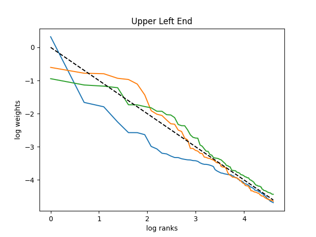
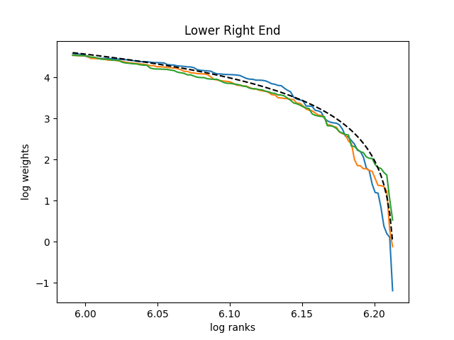
Figure 4: Simulated capital distribution curves. Left panel: \((-\ln k, -\ln\tau_k)\) for \(k = 1, \ldots, 100\) and \(y = -x\) for \(x \in[0, \ln100]\). Right panel: \((\ln(501-k), -\ln\tau_k)\) for \(k = 1, \ldots, 100\) and \(y = \ln(500 - e^x)\) for \(x \in[\ln 401, \ln 500]\). For each panel, 3 simulations (solid) and the deterministic function (dotted)..
The next lemma is the key to our analysis of both ends of the standard normal curve 40 . It is proved very similarly to our results in [26], but we provide the full proof for completeness.
Lemma 3. With probability \(1\), the sequence \(|\ln\tau_k - \ln k|,\, k = 1, 2, \ldots\) is bounded.
Proof. From [22], we know that the random variables \(\ln\tau_k - \ln\tau_{k-1}\) are independent. By Lemma 2, the mean of \(\ln\tau_{k+1} - \ln\tau_k\) is \(1/k\) and the variance is \(1/k^2\). These differences \(\ln\tau_{k+1} - \ln\tau_k\) all are independent. Therefore, \[\label{eq:sums} \mathbb{E}\left[\ln\tau_k\right] = \sum_{j=1}^k\frac{1}{j} =: S(k),\quad \mathrm{Var}\left[\ln\tau_k\right] = \sum_{j=1}^k\frac{1}{j^2} := V(k).\tag{50}\] It is well-known that \(S(k) \sim \ln k\) as \(k \to \infty\), and the sequence \((S(k) - \ln k)\) is bounded. Also, \(V(k) \to \pi^2/6\) as \(k \to \infty\). By [27], from 50 we complete the proof. ◻
Thus we can replace \(\ln\tau_k\) in 45 with \(\ln k\). This result allows us to approximate the curve 45 with
continuous functions. The upper-left end of the curve 45 then becomes \((\ln k, -\ln k)\). This is a linear curve with 45 degrees of incline. Next, the lower-right end of the curve
becomes \((\ln k, \ln(N+1-k))\). Let \(x = \ln k\) and \(y = \ln(N+1-k)\): Then \[y = \ln(a - e^x),\quad a := N+1.\] This
function is concave but obviously not linear: \[y'' = \left(\frac{(a-e^x)'}{a - e^x}\right)' = \left(1 + \frac{a}{e^x-a}\right)' = -\frac{ae^x}{(e^x-a)^2} < 0.\] In light of all this, we reproduce
the shape of this capital distribution curve. See Figure 4 for the upper left and lower right ends of the capital distribution curve. The simulation of \(\ln\tau_k\) for \(k = 1, \ldots, 100\) and the plot of the comparative deterministic function (with \(N = 500\)) was done in Python. The code
standard-curve-simulation.py is in GitHub repository asarantsev/size-capm-vix The shape of both ends of the curve in Figure 3 are reproduced here in
Figure 4.