Shortest Path Lengths in Poisson Line Cox Processes: Approximations and Applications
November 25, 2024
Abstract
We study street-constrained (\(\ell_1\)) shortest paths in a Poisson line Cox process (PLCP), where Poisson points of linear intensity \(\mu\) lie on the lines of an underlying Poisson line process (PLP) of density \(\lambda\). Under a one-turn restriction, we derive closed-form expressions for the distribution of the nearest-neighbor path length from (i) the typical PLCP point and (ii) the typical PLP intersection, by explicitly evaluating the relevant void probabilities via a geometric decomposition of the feasible path-length set. For the intersection case, we further provide analytically tractable upper and lower bounds that capture the impact of \(\lambda\) and \(\mu\). Allowing two turns from the typical point, we obtain a computable upper bound using a feasible-set shrinking argument and identify regimes in which it is tight. We also delineate parameter ranges where a one-turn route from a typical intersection can outperform a two-turn route from a typical point. Finally, we discuss how the results enable statistical performance characterization of ride-hailing services in terms of service guarantee, trip time, and consequently, derive dimensioning insights. We also illustrate qualitatively, how the results can be employed to study vehicle-to-vehicle communication broadcast messages near intersections.
Line process, point process, Cox process, path lengths, stochastic geometry, road transportation.
1 Introduction↩︎
Line or hyperplane processes are critical statistical models used to address various engineering issues in transportation and urban infrastructure planning, wireless communications, and industrial automation [1], [2]. In the Euclidean plane, these processes represent the set of points that constitute lines on the plane, where, the locations and orientations of the lines are specified on a parameter space according to a spatial point process. In particular, the PLP is a stochastic model used to describe random patterns of lines on a plane, where the lines are generated by a PPP in the parameter space. Researchers utilize line processes to investigate doubly stochastic processes called Cox processes, which are Poisson point processes constrained on the line process as their domain [3]–[7]. These models are instrumental in solving engineering questions, such as planning for the number of electric vehicle charging stations and bus stops, analyzing the cellular coverage performance for urban users with on-street deployments of wireless small cells [8], etc.
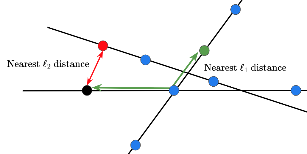
The \(\ell_1\) distance is a metric that measures the shortest path between two points when the movement is restricted to the lines of the PLP. This is particularly important for transportation networks since it characterizes the distance traveled by a vehicle or pedestrian along the streets. Despite the relevance of this metric for practical applications, the characteristics and computational methods for \(\ell_1\) distances in the PLCP are not well understood. Let \(\Phi\) denote the PLCP on \(\mathbb{R}^2\) and let \(\mathbf{o}\) be the typical location (e.g., either the typical point or the typical intersection). The \(\ell_2\) (Euclidean) distance to the nearest PLCP point is \(R \triangleq \inf_{\mathbf{x}\in\Phi} \lVert \mathbf{x}-\mathbf{o} \rVert_2\). Fig. 1 illustrates the difference between the nearest neighbor with respect to the Euclidean distance in contrast to the same in terms of the path length. Although the nearest \(\ell_2\) distance is simple to derive, e.g., see [8], [9], the same is not true for the shortest path-length or the \(\ell_1\) distance.
Researchers have studied the shortest path length distributions for the case of the Manhattan line Cox process [10], where the orientations of the lines are restricted to a discrete set of two angles \(\{0,\pi/2\}\). This was further extended to study dynamic charging of electric vehicles in [11]. For the PLCP model, the authors of [12] have proposed a method for simple computation of the mean shortest path lengths leveraging Neveu’s exchange formula [13]. The asymptotic behavior of this shortest path distance is investigated in [14]. However, due to the random orientation of the lines in a PLP, the exact characterization of the distribution of the shortest path length is challenging, and is still an open problem.
1.1 Contributions↩︎
The main contributions of this paper are summarized as follows.
Exact single-turn distance distribution from the typical point: Under the restriction of at most one turn, we derive a closed-form expression for the CDF of the shortest path length from the typical point of a PLCP to its nearest neighbor. The derivation is based on an explicit evaluation of the void probability via conditioning on the underlying PLP and exploiting the conditional independence of the one-dimensional PPPs defined on distinct lines.
Exact single-turn distance distribution from the typical intersection: We establish an exact characterization of the shortest path length distribution when the origin is the typical intersection of the PLP. This requires a detailed geometric decomposition of the feasible path-length region along intersecting random lines and a case-by-case evaluation of the corresponding void probabilities. The resulting expression captures the interaction between line orientation randomness and point process density.
Upper and lower bounds for the intersection case: We derive analytically tractable lower and upper bounds on the shortest path length distribution from the typical intersection. These bounds are obtained by systematically enlarging or shrinking the feasible path set and provide interpretable performance limits in terms of the line density \(\lambda\) and point density \(\mu\).
Two-turn analysis via feasible-set shrinking: For the two-turn case starting from the typical point, we derive an explicit upper bound on the shortest path length distribution. The bound is obtained through a feasible-set shrinking argument, whereby only a subset of admissible two-turn paths is considered to ensure tractability. This yields a computable expression that captures the impact of additional routing flexibility while preserving analytical rigor.
Transportation-system performance metrics: We formally connect the derived shortest path length distributions to transportation-relevant metrics, including accessibility probability and expected distance in urban street networks modeled by PLCPs. We further quantify the discrepancy between Euclidean-distance-based planning and street-constrained planning, providing explicit analytical expressions for the accessibility gap and detour bias as functions of \(\lambda\) and \(\mu\).
Finally, we show qualitatively how our results will find applications both in wireless network analysis, especially in vehicular communications. We discuss two such applications, one on near-field broadcasting of basic safety messages leveraging RISs and the other on planning for the placement of electric vehicle charging points.
2 Background and Notation↩︎
A line process in \(\mathbb{R}^2\) is a set of points in \(\mathbb{R}^2\) that constitute a set of lines. Each line \(L_i\) is uniquely characterized by its signed distance \(r_i\) from the origin and the angle \(\theta_i\) that the normal to the line makes with the \(x-\)axis. The parameter pair \((\theta_i, r_i)\) thus resides as a point in a parameter space \([0, \pi) \times (-\infty, \infty)\) that generates the line \(L_i\) in \(\mathbb{R}^2\).
Definition 1. A line process \(\mathcal{P} \subset \mathbb{R}^2\) is called a PLP iff the generating points form a PPP on the parameter space \([0, \pi) \times (-\infty, \infty)\) with a constant density \(\lambda\).
On each \(L_i \subset \mathcal{P}\), let us define a one dimensional PPP \(\Phi_i \subset L_i\) with intensity \(\mu\). The collection of all such one dimensional PPPs on all such lines \(\Phi \coloneq \cup_{i: L_i \subset \mathcal{P}} \Phi_i\) is called a PLCP with intensity parameters \(\lambda\) and \(\mu\). Furthermore, we denote by \(I_{ij}\) as the point of intersection of \(L_i\) and \(L_j\), and define the intersection process as \(\Phi_{\rm I} \coloneq \cup_{i,j: L_i,L_j \subset \mathcal{P}} I_{ij} = \cup_{i,j \in \mathcal{P}} L_i \cap L_j\). We perform our analysis from the perspective of the typical point of \(\Phi\). In particular, let us define \[\begin{align} \Phi^o\triangleq(\Phi\mid o\in\Phi), \nonumber \end{align}\] and note that under expectation over \(\Phi^o\), \(o\) becomes the typical point of the process \(\Phi\). Since by construction, \(\Phi\) is a stationary process, let us consider \(o\) to be the origin of \(\mathbb{R}^2\). Under Palm conditioning, there exists a line \(L_{\rm x}\) passing through \(o\). Without loss of generality, let us consider \(L_{\rm x}\) to be the \(x-\)axis. Let the lines intersecting \(L_{\rm x}\) be enumerated (in no particular order) by the elements of the set \(\{L_i\}\), \(i \in \mathbb{N}\) and the corresponding intersections be \(\{I_i\}\). Let the distance of \(I_i\) from the origin be denoted by \(s_i\) and the angle between \(L_1\) and \(L_{\rm x}\) be denoted by \(\theta_i\). Let \(D\) denote the length of the shortest path from the typical point to the nearest neighbor of the PLCP. Mathematically, \(D = \min_{x\in\Phi^{!o}} \|x\|_1,\) where \(\Phi^{!o}\) is the reduced Palm process constructed by assuming the typical point to be a part of \(\Phi\) and then by removing the typical point.
2.1 Limitation of a trivial approximation↩︎
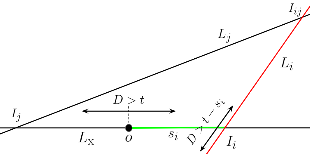
Note that a simple approximation as illustrated in Fig. 2 follows by assuming that the distribution of the shortest path length from the typical PLCP point is the same as the distribution of the shortest path length from \(I_i\) conditioned on the event that the path from \(I_i\) cannot start along \(L_{\rm x}\) but along \(L_{i}\). In Fig. 2 it means that at \(I_i\), we remove the line \(L_{\rm x}\) and consider \(I_i\) as the surrogate of the typical point and study the event \(D > t- s_i\). Mathematically, this results in the following recursive equation. \[\begin{align} \mathbb{P}(D>t)=& \exp\left(-\mu t\right) \sum_k p_k(t) \left(\frac{1}{t}\int_{0}^{t}\mathbb{P}(D>t-s)\, ds\right)^k, \nonumber \end{align}\] where \(p_k(t)\coloneq \exp\left({-2\lambda t}\right) \frac{(2\lambda t)^k}{k!},\) is the probability that there are \(k\) intersections within a distance \(t\) from the typical point. Conditioned on \(k\), the distances of these intersections are independent and identically (in fact uniformly) distributed in \([0,t]\). As per the approximation, given that an intersection is at a distance \(s\) from the typical point on \(L_{\rm x}\), for no points within a path length \(t\) from the typical point, we are interested in the event \(D > t -s\) from the intersection. Thus, we get \[\begin{align} \mathbb{P}(D>t) = \exp\left(-\mu+2\lambda\right) t \sum_k \frac{1}{k!} \left(2\lambda \int_{0}^{t}\mathbb{P}(D>t-s)\, d{\rm s}\right)^k, \nonumber \end{align}\] Now defining \(u(t) \coloneq \mathbb{P}(D>t)\), \(I(t) \coloneq \int_{0}^{t}u(t-s)\, d{\rm s}\) and differentiating with respect to \(t\) we obtain the following differential equation. \[\begin{align} u'(t)&=\exp\left(-(\mu+2\lambda) t\right)\sum_k \frac{1}{(k-1)!} \left(2\lambda \int_{0}^{t}u(t-s)\, {\rm d}s\right)^{k-1} \nonumber \\ &\frac{{\rm d}}{{\rm d}t}\left(2\lambda \int_{0}^{t}u(t-s)\, ds\right) -(\mu+2\lambda)u(t) \nonumber \\ &=\exp\left({-(\mu+2\lambda) t}\right) 2\lambda \sum_k \frac{1}{(k-1)!} \nonumber \\ & \left(2\lambda t \int_{0}^{t}u(t-s)\, ds\right)^{k-1} -(\mu+2\lambda)u(t) \nonumber\\ &= 2\lambda u(t) -(\mu+2\lambda)u(t) = -\mu u(t). \nonumber \end{align}\] This solution results in \(\mathbb{P}\left(D > t\right) = \exp(-\mu t)\), which is incidentally the same as the probability of no PLCP point being located within a distance \(t\) on \(L_{\rm x}\) from the typical point. This occurs due to the fact that while approximating the path length from \(I_{i}\) to be \(D\), we over-count segments of the PLP, e.g., the segment between the typical point and \(I_i\) shown in green in Fig. 2. This motivates the need for a more careful characterization of the path length distribution.
3 Single Turn Case↩︎
Let us first consider the restriction that only those PLCP points are accounted for that are reachable by traversing at most two lines \(L_i\), including \(L_{\rm x}\). Within this restriction, we consider two cases: first where the origin is the typical point and second where the origin is the typical intersection.
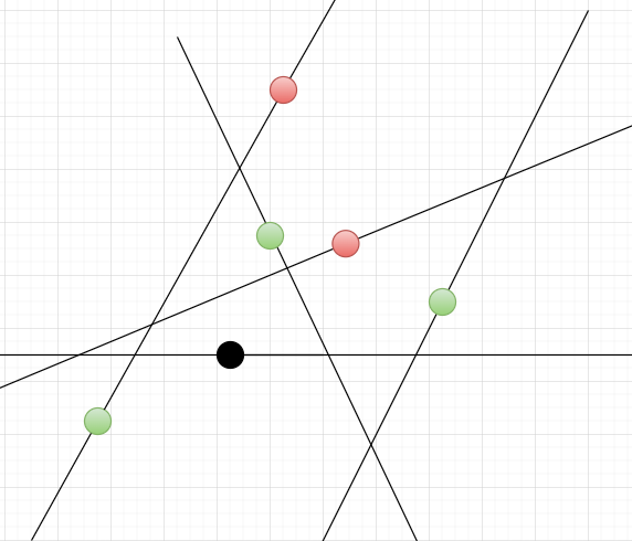
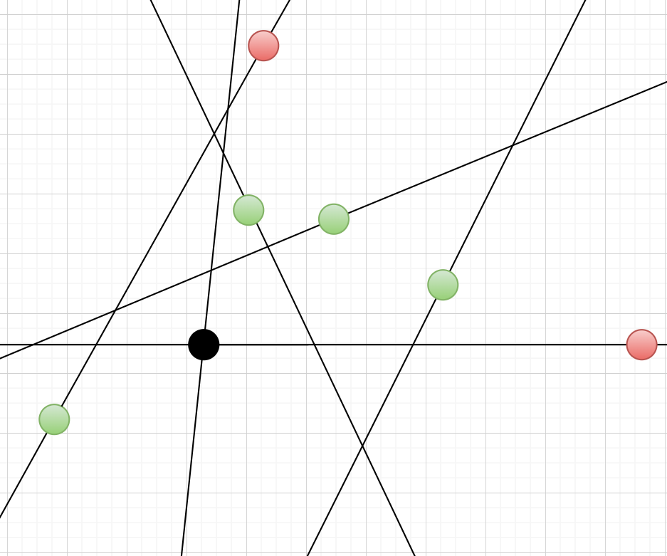
Figure 3: All the green colored points are within a distance \(t\) by taking at most one turn from the origin (black point) when (a) the origin is the typical point of the PLCP and (b) the origin is the typical intersection of the PLP..
3.1 From the typical point↩︎
Let the number of intersections from the origin within a distance \(t\) be \(N_t\). Furthermore, let \([N_t]\) denote the set \(\{1, 2, \ldots, N_t\}\). As per the property of PLP, \(N_t\) is Poisson distributed with intensity \(2\lambda t\) [4]. Accordingly, the CCDF of \(D\) is evaluated as one minus the void probability.
Theorem 1. Restricted to the single turn case, the distribution of the shortest path length from the typical point of the PLCP to another point of the PLCP is \[\begin{align} F_D(t) = 1 - \exp\left(-2\mu t - 2 \lambda t + \frac{\lambda}{\mu}\left(1 - \exp\left(-2\mu t\right)\right)\right). \label{eq:one95turn95CDF} \end{align}\qquad{(1)}\]
The shortest path length distribution follows directly from the void probability \(\mathbb{P}(D > t)\). Conditioned on \(\mathcal{P}\), the point processes \(\{\Phi_i\}_{L_i \in \mathcal{P}}\) defined on distinct lines are independent one-dimensional PPPs with intensity \(\mu\). Hence, conditioned on \(\mathcal{P}\), events corresponding to disjoint path-length segments on different lines are independent.
Using the counting measure notation for point processes [15], where \(\Phi(A)\) denotes the number of points of \(\Phi\) within a path length \(A\), and letting \(\Phi_{\rm x}\) denote the PPP on \(L_{\rm x}\), we first evaluate the conditional void probability: \[\begin{align} \mathbb{P}(D > t \mid \mathcal{P}) &= \mathbb{P}\!\left(\Phi_{\rm x}(t)=0, \bigcup_{i:s_i\le t}\Phi_i(t-s_i)=0 \,\middle|\, \mathcal{P}\right). \end{align}\]
By conditional independence of the point processes on distinct lines, \[\begin{align} \mathbb{P}(D > t \mid \mathcal{P}) &= \mathbb{P}\!\left(\Phi_{\rm x}(t)=0 \mid \mathcal{P}\right) \prod_{i:s_i\le t} \mathbb{P}\!\left(\Phi_i(t-s_i)=0 \mid \mathcal{P}\right). \end{align}\] In what follows, we first condition on the PLP, then exploit the conditional independence pf the PPPs across different lines, and finally apply the law of total expectation. Since each \(\Phi_i\) is a one-dimensional PPP with intensity \(\mu\), the conditional void probabilities are \[\mathbb{P}\!\left(\Phi_{\rm x}(t)=0 \mid \mathcal{P}\right)=\exp(-2\mu t),\] and \[\mathbb{P}\!\left(\Phi_i(t-s_i)=0 \mid \mathcal{P}\right) =\exp\big(-2\mu (t-s_i)\big).\]
Therefore, \[\begin{align} \mathbb{P}(D > t \mid \mathcal{P}) &= \exp(-2\mu t) \prod_{i:s_i\le t} \exp\big(-2\mu (t-s_i)\big). \end{align}\]
The unconditional void probability is then obtained by applying the law of total expectation with respect to the distribution of the PLP: \[\begin{align} \mathbb{P}(D > t) &= \mathbb{E}_{\mathcal{P}} \left[ \exp(-2\mu t) \prod_{i:s_i\le t} \exp\big(-2\mu (t-s_i)\big) \right]. \end{align}\]
Now, the number of lines intersecting \(L_{\rm x}\) within distance \(t\) is Poisson distributed with mean \(2\lambda t\), and conditioned on this number being \(k\), the intersection locations \(\{s_i\}\) are i.i.d. uniform on \([0,t]\). Hence, \[\begin{align} \mathbb{P}(D > t) &= \exp(-2\mu t) \sum_{k=0}^{\infty} \frac{\exp(-2\lambda t)(2\lambda t)^k}{k!} \nonumber \\ &\left( \frac{1}{t}\int_0^t \exp(-2\mu(t-s))\,{\rm d}s \right)^k. \end{align}\]
Evaluating the geometric series yields \[\begin{align} \mathbb{P}(D > t) = \exp\left(-2\mu t - 4\lambda t + \frac{2\lambda}{\mu}\left(1-\exp(-2\mu t)\right) \right). \end{align}\]
Finally, one minus the void probability gives the required distance distribution.
Remark 1. Note that the expression for the void probability is composed of three different terms: \(\exp\left(-2\mu t\right)\) that represents the probability that no PLCP points is present within \(t\) in \(L_{\rm x}\); the term \(\exp\left(-4\lambda t\right)\) corresponds to the event that no line intersects within a distance \(t\) from the typical point; while, considering the fact that for the void event, lines can intersect within \(t\) as long as they do not contain any points within a distance \(t -s_i\), the second term is weighted by the positive quantity \(\exp\left(\frac{2\lambda}{\mu}(1 - \exp(-2 \mu t))\right)\).
3.2 From the typical intersection↩︎
Next, let us consider the typical intersection \(O\) depicted in Fig. 4. Here, unlike the previous case, under Palm conditioning, there exists two lines passing through the typical intersection, denoted by \(L_{\rm x}\) and \(L_{\rm y}\), respectively. To be precise, we define the conditioned line process \(\mathcal{P}^o\) as \[\begin{align} \mathcal{P}^o \triangleq (\mathcal{P} | L_{\rm x}, L_{\rm y} \in \mathcal{P}), \end{align}\] where \(L_{\rm x}\) and \(L_{\rm y}\) are two lines with a uniformly distributed angle of intersection. Then, under expectation over \(\mathcal{P}^o\), the intersecting point \(O\) becomes the typical intersection. Let the angle between \(L_{\rm x}\) and \(L_{\rm y}\) be \(\theta\). Let the random variable \(Z_1\) denote the length of the lines of \(\mathcal{P}\) wherein no point of \(\Phi\) should be present for the event \(D > t\) to hold. First, we characterize \(Z_1\) for different cases of intersection locations of lines \(L_1\) on \(L_{\rm x}\) and \(L_{\rm y}\). Then, we average out over all possible such \(L_1\) within \(t\) to obtain the final result.
Theorem 2. The distribution of the distance to the nearest PLCP point from the typical intersection of the PLP is \[\begin{align} F_D(t) = 1 - \exp\left( - 4 \mu t - 2\lambda \left(2t - \mathcal{T}_x - \mathcal{T}_y\right)\right), \end{align}\] where \[\begin{align} \mathcal{T}_x =\frac{1}{\pi^2} \int_0^\pi \int_0^t \int_0^\pi \exp\left(-\mu Z(x, \omega_1, \omega)\right) {\rm d}\omega_1 {\rm d}x {\rm d}\omega, \nonumber \\ \mathcal{T}_y =\frac{1}{\pi^2} \int_0^\pi \int_0^t \int_{\theta_{\mathcal{E}_{1,1}}}^{\theta_{\mathcal{E}_{1,2}}} \exp\left(-\mu Z(x, \omega_1, \omega)\right) {\rm d}\omega_1 {\rm d}x {\rm d}\omega, \nonumber \end{align}\] and \[\begin{align} &Z(x, \omega_1, \omega) = \nonumber \\ &\begin{cases} 2t - x \left(\frac{\sin \omega - \sin \omega_1}{\sin (\omega_1 - \omega)} +1 \right); \omega_1 \in [0, \theta_{\mathcal{E}_{2,1}}] \cup [\theta_{\mathcal{E}_{2,2}}, \pi] \nonumber \\ 2(t - x); \quad \theta_1 \in [\theta_{\mathcal{E}_{1,1}}, \theta_{\mathcal{E}_{1,2}}] \nonumber \\ 4t - 2x\left(1 + \frac{2\sin \omega_1}{\sin (\omega_1 - \omega)}\right); \omega_1 \in [\theta_{\mathcal{E}_{2,1}}, \theta_{\mathcal{E}_{1,1}}] \cup [\theta_{\mathcal{E}_{1,2}}, \theta_{\mathcal{E}_{2,2}}]. \end{cases} \end{align}\] The ranges of \(\theta_1\) in the above equation are as follows. \[\begin{align} &\theta_{\mathcal{E}_{1,1}} = \arctan \left(\frac{t\sin \omega}{ t\cos \omega - x}\right), \nonumber \\ & \theta_{\mathcal{E}_{1,2}} = \arctan\left(\frac{t\sin \omega}{x + t\cos \omega}\right),\nonumber \\ &\theta_{\mathcal{E}_{2,1}} = \arccos \left(\frac{\left(\left(\frac{2t - x}{x}\right)^2 + 1\right) \cos \omega + 2\left(\frac{2t - x}{x}\right) }{2\left(\frac{2t - x}{x}\right)\cos\omega + \left(\frac{2t - x}{x}\right)^2 + 1}\right), \nonumber \\ &\theta_{\mathcal{E}_{2,2}} = \arccos \left(\frac{\left(\left(\frac{2t - x}{x}\right)^2 + 1\right) \cos \omega - 2\left(\frac{2t - x}{x}\right) }{-2\left(\frac{2t - x}{x}\right)\cos\omega + \left(\frac{2t - x}{x}\right)^2 + 1}\right).\nonumber \end{align}\]
From the typical intersection, under the restriction of at most one turn, we can traverse either \(L_{\rm x}\) or \(L_{\rm y}\), but not both. Its worth recalling that conditioned on \(\mathcal{P}\), the point processes defined on distinct lines are independent one-dimensional PPPs with intensity \(\mu\). Additionally, note that across realizations of \(\mathcal{P}^o\), all the other lines almost surely intersect both \(L_{\rm x}\) and \(L_{\rm y}\). Let us consider one such line, \(L_1\), that intersects \(L_{\rm x}\) at \(P'\) at a distance \(s_1\) from the origin and \(L_{\rm y}\) at \(Q'\) at a distance \(s'_1\) from the origin. Naturally, \[\begin{align} s'_1 = \frac{s_1\sin \theta_1}{\sin(\theta_1 -\theta)}. \label{eq:s2} \end{align}\tag{1}\] The length of the segment of intersection \(|P'Q'|\) has two equivalent forms for given \(s_1\), \(\theta\), and \(\theta_1\): \[\begin{align} |P'Q'| &= \frac{s_1 \sin \theta}{\sin (\theta_1 - \theta)} = \frac{s'_1 \cos \theta - s_1 }{\cos \theta_1}, \label{eq:PQ2} \end{align}\tag{2}\] where \(s'_1\) is given by 1 . Now conditioned on \(\theta\) and \(s_1\) consider the following events: (i) the event \(\mathcal{E}^c_1\) (complement of event \(\mathcal{E}_1\)) defined as the case \(s'_1 > t\). In this case, for the shortest path to be of length less than \(t\) and the corresponding point to lie on \(L_1\), the path can only be via the intersection \(I_{{\rm x}1}\) and not via \(I_{{\rm y}1}\); and (ii) the joint event \(\mathcal{E}_2 \mathcal{E}_1\) defined as \(|P'Q'| \leq (t-s_1) + (t - s'_1)\) and \(s'_1 \leq t\). In this case, the both \(I_{{\rm x}1}\) and \(I_{{\rm y}1}\) are feasible intersection points distances less than \(t\) on \(P'Q'\). We convert the above conditions on \(s'_1\) to corresponding conditions on \(\theta_1\), given \(s_1\) and \(\theta\). Note that \(\theta_1 = \arctan \left(\frac{s'_1\sin \theta}{s'_1\cos \theta - s_1}\right)\). Thus, for \(s'_1 > t\), we have \[\begin{align} \theta_1 > \arctan \left(\frac{t\sin \theta}{ t\cos \theta - t}\right) = \theta_{\mathcal{E}_{1,1}}. \label{eq:phiE11} \end{align}\tag{3}\] Similarly, let \(\theta_{\mathcal{E}_{1,2}}\) be the angle for which \(L_1\) intersects \(L_{\rm y}\) at a distance \(t\) from the origin below the x-axis. For that case, we find a similar angle \(\theta_{\mathcal{E}_{1,2}} = \arctan\left(\frac{t\sin \theta}{s_1 + t\cos \theta}\right)\). Thus, the event \(\mathcal{E}^c_1\) is equivalent to \(\theta_1 \in (\theta_{\mathcal{E}_{1,1}},\theta_{\mathcal{E}_{1,2}})\). Since for the event \(\mathcal{E}^c_1\), any point within a distance \(t\) on \(L_1\) is reachable only from the \(I_{{\rm x}1}\) intersection, for such a point to not exist, we calculate the void probability in a segment of length \(Z_1(s_1, \theta, \phi) = 2(t - s_1)\) on \(L_1\).
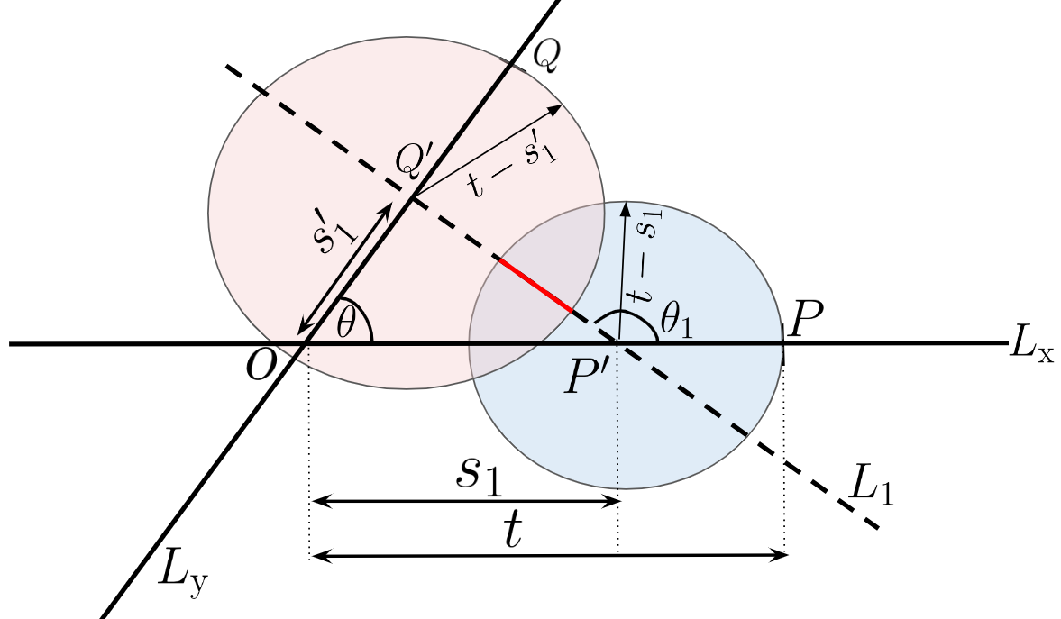
Next let us study the event \(\mathcal{E}_1\mathcal{E}_2\). Following the same steps as before, we note that if \(L_1\) intersects \(L_{\rm y}\) above the \(x-\)axis, then the event \(\mathcal{E}_2\) corresponds to \(\frac{s'_1\sin \theta}{\sin (\theta_1 - \theta)} < 2t - s_1 - \frac{s_1}{\sin (\theta_1 - \theta)}\), or \[\begin{align} \pi \geq \theta_1 &> \arccos \left(\frac{\left(\left(\frac{2t - s_1}{s_1}\right)^2 + 1\right) \cos \theta - 2\left(\frac{2t - s_1}{s_1}\right) }{-2\left(\frac{2t - s_1}{s_1}\right)\cos\theta + \left(\frac{2t - s_1}{s_1}\right)^2 + 1}\right) \nonumber \\ &= \theta_{\mathcal{E}_{2,2}}. \label{eq:phiE22} \end{align}\tag{4}\] On the contrary, in case \(L_1\) intersects \(L_{\rm y}\) below the \(x-\)axis, the event \(\mathcal{E}_2\) corresponds to \[\begin{align} 0 \leq \theta_1 &\leq \arccos \left(\frac{\left(\left(\frac{2t - s_1}{s_1}\right)^2 + 1\right) \cos \theta + 2\left(\frac{2t - s_1}{s_1}\right) }{2\left(\frac{2t - s_1}{s_1}\right)\cos\theta + \left(\frac{2t - s_1}{s_1}\right)^2 + 1}\right) \nonumber \\ &=\theta_{\mathcal{E}_{2,1}}. \label{eq:phiE21} \end{align}\tag{5}\] Thus, the joint event \(\mathcal{E}_1\mathcal{E}_2\) corresponds to \(\theta_1 \in [0, \theta_{\mathcal{E}_{2,1}}) \cup (\theta_{\mathcal{E}_{2,2}}, \pi]\). For this case, the length of interest on \(L_1\) where no points should reside is evaluated as \[\begin{align} Z_1(s_1, \theta, \theta_1) = 2t - s_1 \left(\frac{\sin \theta + \sin \theta_1}{\sin (\theta_1 - \theta)} +1 \right). \label{eq:ZE1E2} \end{align}\tag{6}\] Finally, for the event \(\mathcal{E}_1\mathcal{E}^{\rm c}_2\), we have \(\theta_1 \in [\theta_{\mathcal{E}_{2,1}}, \theta_{\mathcal{E}_{1,1}}] \cup [\theta_{\mathcal{E}_{1,2}}, \theta_{\mathcal{E}_{2,2}}]\). In this case, \[\begin{align} Z_1(s_1, \theta, \theta_1) = 4t - 2s_1\left(1 + \frac{\sin \theta_1}{\sin (\theta_1 - \theta)}\right). \label{eq:ZE1E2c} \end{align}\tag{7}\]
Let \(\mathcal{P}_{\rm x} \subset \mathcal{P}\) denote the set of lines that intersect \(L_{\rm x}\) within a distance \(t\) from the origin. Furthermore, let \(\mathcal{P}'_{\rm y} \subset \mathcal{P}\) denote the set of lines that intersect \(L_{\rm y}\) within a distance \(t\) from the origin and intersect \(L_{\rm x}\) outside a distance \(t\) from the origin. Based on the above characterization, we proceed with our derivation of the void probability as follows. \[\begin{align} &\mathbb{P}\left(D > t\right) = \mathbb{P}\left(\Phi_{\rm x}(t) = 0, \Phi_{\rm y}(t) = 0, \cup_{\mathcal{P}_{\rm x}}\Phi_i(t - s_i)\right. \nonumber \\ &\left.\cup_{\mathcal{P}'_{\rm y}} \Phi_j(t - s'_i) = 0 \right) \nonumber \\ &=\mathbb{P}\left(\Phi_{\rm x}(t) = 0\right)\mathbb{P}\left(\Phi_{\rm y}(t) = 0\right) \mathbb{P}\left(\Phi \cap \left(\cup_{i \in \mathcal{P}_{\rm x}} Z_i\right) = 0\right)\nonumber \\ &\mathbb{P}\left(\Phi \cap \left(\cup_{i \in \mathcal{P}'_{\rm y}} Z_i\right) = 0\right) \nonumber \\ &=\exp\left(- 4 \mu t\right) \cdot \nonumber \\ &\left[\sum_{k = 0}^\infty \frac{p_k(t)}{\pi^2 t} \left( \int_0^\pi \int_0^t \int_0^\pi \exp\left(-\mu Z(x, \omega_1, \omega)\right)d\omega_1 {\rm d}x {\rm d}\omega\right)^k\right]\nonumber \\ & \left[\sum_{k = 0}^\infty \frac{p_k(t)}{\pi^2 t} \left(\int_0^\pi \int_0^t \int_{\phi_{\mathcal{E}_{1,1}}}^{\phi_{\mathcal{E}_{1,2}}} \exp\left(-\mu Z(x, \omega_1, \omega)\right) \right.\right. \nonumber \\ &\left.\left. {\rm d}\omega_1 {\rm d}x d\omega\right)^k\right] \nonumber \\ & = \exp\left( - 4 \mu t - 2\lambda \left(2t - \mathcal{T}_x - \mathcal{T}_y\right)\right). \end{align}\]
Remark 2. In Theorem 2, the term \(\exp(-4\mu t)\) corresponds to the probability that no point located in either \(L_{\rm x}\) or \(L_{\rm y}\) within a distance \(t\). The term \(\exp(-4\lambda t)\) is the probability that no lines should be present with a distance \(t\) from the origin along \(L_{\rm x}\) or \(L_{\rm y}\). However, for the void event such lines can be present given that they do not contain any PLCP points within a path length \(t\) from the origin. Consequently, the probability is augmented by the factor \(\exp(2\lambda\mathcal{T}_{\rm x}) \cdot \exp\left(2 \lambda \mathcal{T}_{\rm y}\right)\). The first term takes into account the region along the lines of \(\mathcal{P}_{\rm x}\) while the second term does so for the lines of \(\mathcal{P}'_{\rm y}\).
Corollary 1 (Zero Turn Case). The CDF of \(D\) is lower bound as \[\begin{align} F_D(t) \geq 1 - \exp\left(-4\mu t\right). \end{align}\]
This is derived by considering the void probability of \((\Phi_{\rm x} \cup \Phi_{\rm y}) \cap \mathcal{B}(0, t)\), where \(\Phi_{\rm x}\) and \(\Phi_{\rm y}\) respectively represent the points of \(\Phi\) on \(L_{\rm x}\) and \(L_{\rm y}\), and \(\mathcal{B}(0, t)\) represents a ball of radius \(t\) centered at the typical intersection.
Corollary 2 (Upper bound). The CDF of \(D\) is upper bound as \[\begin{align} F_D(t) \leq 1 - \exp\left(-4(\mu + 4\lambda)t\right). \end{align}\]
The upper bound is derived by considering the void probability of \((\Phi_{\rm x} \cup \Phi_{\rm y} \cup \Phi_{\rm Ix} \cup \Phi_{\rm Iy}) \cap \mathcal{B}(0, t)\), where \(\cup \Phi_{\rm Ix}\) and \(\cup \Phi_{\rm Iy}\) are the intersection in \(\Phi_{\rm I}\) present along \(L_{\rm x}\) and \(L_{\rm y}\), respectively.
The above completes an exact characterization of the distribution of the distance to the nearest PLCP point from either the typical point or from the typical intersection restricted to one turn. The next section extends these results to approximate the two-turns case.
4 Two Turns From The Typical Point↩︎
For the two turns case, we restrict our analysis to the case where starting from the origin, we are allowed to move only in a given direction (without loss of generality, let us consider this to be along the positive direction of the x-axis).
Theorem 3. The distribution of the nearest PLCP point from the typical point of the PLCP under the restriction of two-turns along a single direction is bounded as \[\begin{align} \mathbb{P}\left(D \leq t\right) &\leq 1 - \exp\left(-\lambda \int_0^t 2 - \exp\left( -\lambda \int_0^{u} 2 - \right.\right.\nonumber \\ &\left.\left. T(w, u) f_{s_i|s_1}(w) {\rm d}w\right) f_{s_1}(u) {\rm d}u \right), \end{align}\] where, \(f_{s_i|s_1}(w) = \frac{1}{s_1}\) for \(0 \leq w \leq s_1\), \(f_{s_1}(u) = \frac{1}{t}\) for \(0 \leq u \leq t\). The innermost integrand is \[\begin{align} &T(w, u) = \mathbb{1}\left(\mathcal{E}_i\right) \iint_{\theta_i, \theta_1 \in \mathcal{E}_{i}} \exp\left(-\mu \left( t- \right.\right.\nonumber \\ &\left.\left.\left(\frac{u-w}{\cos \theta_i - \sin \theta_i \cot\theta_1} + w\right)\right)\right) {\rm d}\theta_1 {\rm d}\theta_i + \left(1 - \mathbb{1}\left(\mathcal{E}_i\right)\right)\infty. \end{align}\] The event \(\mathcal{E}_i\) is defined with the following conditions on \(\theta_i\) and \(\theta_1\) as follows. \[\begin{align} \mathcal{E}_{i} = \begin{cases} \theta_1 \leq {\rm cot}^{-1} \left(\cos \theta_i - \left(\frac{u - w}{t - w}\right) \csc \theta_i \right); \quad 0 \leq \theta_i \leq \frac{\pi}{2}, \nonumber \\ \theta_1 > {\rm cot}^{-1} \left(\left(\frac{u - w}{t - w} - \cos \theta_i\right) \csc \theta_i \right); \quad \frac{\pi}{2} < \theta_i \leq \pi. \end{cases} \end{align}\]
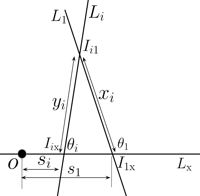
Let us consider the intersection formed by two lines \(L_1\) and \(L_i\) that cross \(L_{\rm x}\) at distances \(s_1\) and \(s_i\), respectively, from the origin such that \(0 \leq s_i \leq s_1 \leq t\). Let us denote by \(x_i\) the distance between the intersection \(I_{i1}\) and \(I_{1X}\). Similarly, \(y_i\) denotes the distance between \(I_{i1}\) and \(I_{iX}\). Naturally, we have \[\begin{align} x_i = \frac{y_i \sin \theta_i}{\sin \theta_1}, \quad \text{ and } y_i = \frac{d_i}{\cos \theta_i - \sin \theta_i \cot\theta_1}. \nonumber \end{align}\] From the intersection \(I_{i1}\), along the line \(L_1\), we have a remaining path-length budget of \(z_i = \max\{0, t - (y_i + s_i)\}\). Thus, we need conditions on \(\theta_1\) and \(\theta_i\) that correspond to the event \(\mathcal{E}_{i} \coloneq \{y_i + s_i \leq t\}\). This evaluates to \[\begin{align} \mathcal{E}_{i} \coloneq \begin{cases} \theta_1 \leq {\rm cot}^{-1} \left(\cos \theta_i - \left(\frac{d_i}{t - s_i}\right) \csc \theta_i \right); \quad 0 \leq \theta_i \leq \frac{\pi}{2}, \nonumber \\ \theta_1 > {\rm cot}^{-1} \left(\left(\frac{d_i}{t - s_i} - \cos \theta_i\right) \csc \theta_i \right); \quad \frac{\pi}{2} < \theta_i \leq \pi. \end{cases} \end{align}\] Accordingly, \(z_i\) takes a value 0 in the event \(\mathcal{E}^c_{i}\) (the event that no path length budget remains once we reach \(I_{1i})\) and a value \(t - (y_i + s_i)\) in the event \(\mathcal{E}_{i}\). Let us denote by \(D_i\) to be the conditional path length \(D\) given that it resides in the line \(L_1\) and is reached via the intersections \(I_{i{\rm x}}\) and \(I_{i1}\). Leveraging the fact that \(\Phi \cap [O, I_{iX}]\) and \(\Phi \cap [I_{iX}, I_{i1} ]\) are independent, we have \[\begin{align} T(s_i, s_1) &= \mathbb{P}\left(D_i \geq t | s_i, s_1\right) = \mathbb{P}\left(\Phi_i((t - (y_i + s_i))^+) = 0\right) \nonumber \\ &= \int_0^{\pi}\int_0^{\pi} \exp\left(-\mu z_i\right) {\rm d}\theta_1 {\rm d}\theta_i \nonumber \\ &= \iint_{\theta_i, \theta_1 \in \mathcal{E}_{i}} \exp\left(-\mu ( t- (y_i + s_i))\right) {\rm d}\theta_1 {\rm d}\theta_i. \nonumber \end{align}\] Next, we take into account all \(s_i\) such that \(0 \leq s_i \leq s_1\). Thanks to the property of the PLP, the number \(n_1\) of such lines is Poisson distributed with parameter \(2s_1 \lambda\). Accordingly, \[\begin{align} T(s_1) &= \mathbb{P}\left( \cup_{i:s_i \leq s_1} \Phi_i((t - (y_i + s_i))^+)= 0\right) \nonumber\\ &= \mathbb{E}_{n1, \{s_i\}}\left[\cup_i T(s_i, s_1)\right] \nonumber \\ &\geq \mathbb{E}_{n_1}\left[\prod_{i = 1}^{n_1} \mathbb{E}_{s_1} \left[T(s_i, s_1)\right]\right] \nonumber \\ &= \sum_{k = 0}^\infty \left(\int_0^{s_1} T(w, s_1) f_{s_i|s_1}(w)\right)^k \frac{\exp(-2\lambda s_1) (\lambda s_1)^k}{k!} \nonumber \\ &=\exp\left( -\lambda \int_0^{s_1} 2 - T(w, s_1) f_{s_i|s_1}(w)\right) {\rm d}w, \nonumber \end{align}\] where \(f_{s_i|s_1}(w) = \frac{1}{s_1}\) for \(0 \leq w \leq s_1\). Finally, we note that the selected line \(L_1\) could be any of the Poisson number of lines between 0 and \(t\). This implies that the void probability is upper bounded by \[\begin{align} \mathbb{P}\left(D > t\right) \geq& \exp\left(-\lambda \int_0^t 2 - \exp\left( -\lambda \int_0^{u} 2 - \right.\right.\nonumber \\ &\left.\left. T(w, u) f_{s_i|s_1}(w) {\rm d}w\right) f_{s_1}(u) {\rm d}u \right) \end{align}\] Finally, the distribution of \(D\) follows from the void probability.
Remark 3. The above expression is obtained by shrinking the feasible set of two-turn paths. In particular, instead of accounting for all possible two-turn trajectories, we restrict attention to a subset in which the second turn occurs only after reaching a selected intermediate line \(L_1\). This restriction reduces the set of admissible paths, thereby increasing the corresponding void probability. Consequently, the resulting distribution provides an upper bound on \(\mathbb{P}(D \leq t)\) rather than an exact characterization.
5 Numerical Results on the Trends of the Shortest Path-Length Distribution↩︎
Here we discuss the accuracy of the analytical results and the approximation derived for the two turn case. All the quantities are presented as unit less since the model is scale invariant.
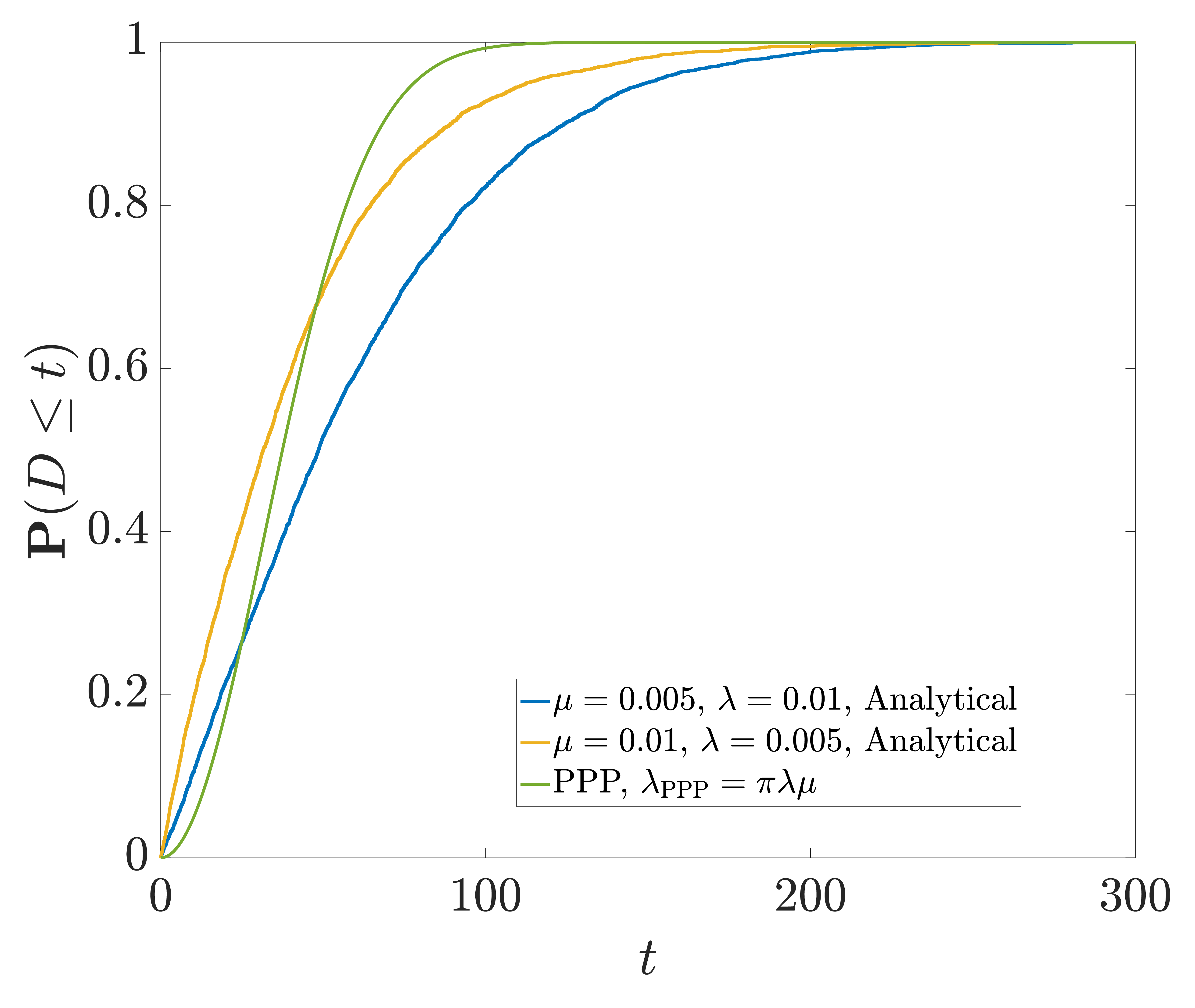
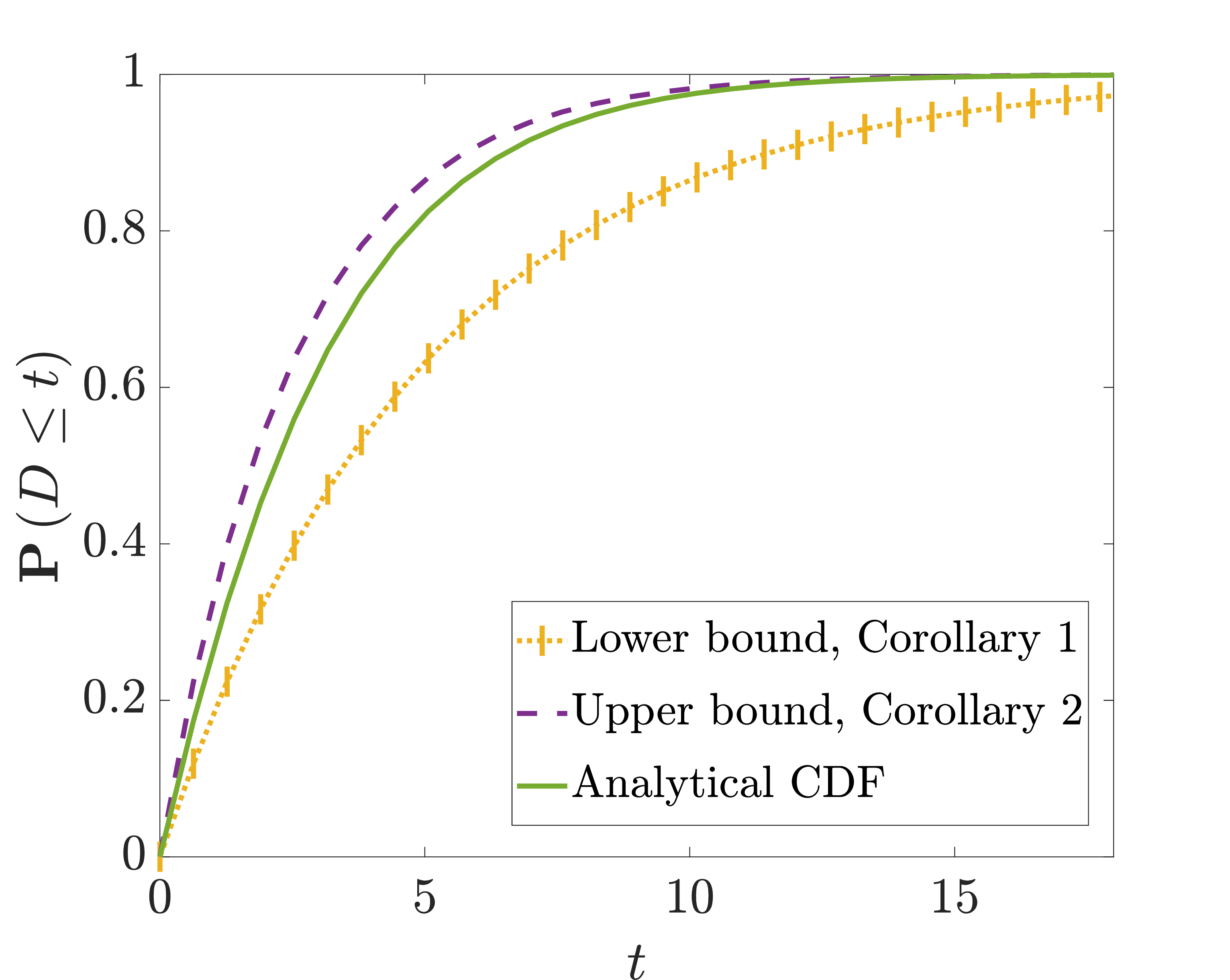
Fig. 6 shows that the distance to the nearest PLCP point is statistically closer from the nearest intersection as compared to the nearest point due to the two possible initial paths \(L_{\rm x}\) and \(L_{\rm y}\) available from the typical intersection as compared to only one path available from the typical point. Furthermore, for comparison, we plot the nearest neighbor distribution for a 2D PPP with intensity \(\lambda_{\rm PPP} = \mu \lambda\). Interestingly, we see that the CDF is lower for the 2D PPP for lower values of \(t\), while the contrary is true for higher values of \(t\). Indeed, due to the fact that a line passes through the typical point of a PLCP, the nearest point can likely be present on such a line. Based on the values of \(\mu\) and \(\lambda\), this may be closer or farther than the nearest neighbor of a 2D PPP with intensity \(\mu \lambda\). However, in case the shortest path to a point is present in a different line than the one passing through the typical PLCP point, its Euclidean distance is smaller than the path length.
Fig. 7 demonstrates the upper and the lower bounds for the shortest path length distribution from the typical intersection as compared to the actual value. Recall that the lower bound is obtained by evaluating the void probability of \((\Phi_{\rm x} \cup \Phi_{\rm y}) \cap \mathcal{B}(0, t)\), where \(\Phi_{\rm x}\) and \(\Phi_{\rm y}\) respectively represent the points of \(\Phi\) on \(L_{\rm x}\) and \(L_{\rm y}\). On the contrary, the upper bound follows from the void probability of \((\Phi_{\rm x} \cup \Phi_{\rm y} \cup \Phi_{\rm Ix} \cup \Phi_{\rm Iy}) \cap \mathcal{B}(0, t)\), where \(\cup \Phi_{\rm Ix}\) and \(\cup \Phi_{\rm Iy}\) are the intersection in \(\Phi_{\rm I}\) present along \(L_{\rm x}\) and \(L_{\rm y}\), respectively. Naturally, the lower bound is tighter when \(\mu\) is higher while the upper bound is tighter when \(\lambda\) is higher. Both the bounds can act as surrogate measures for analysing the performance of wireless networks with low computational complexity.

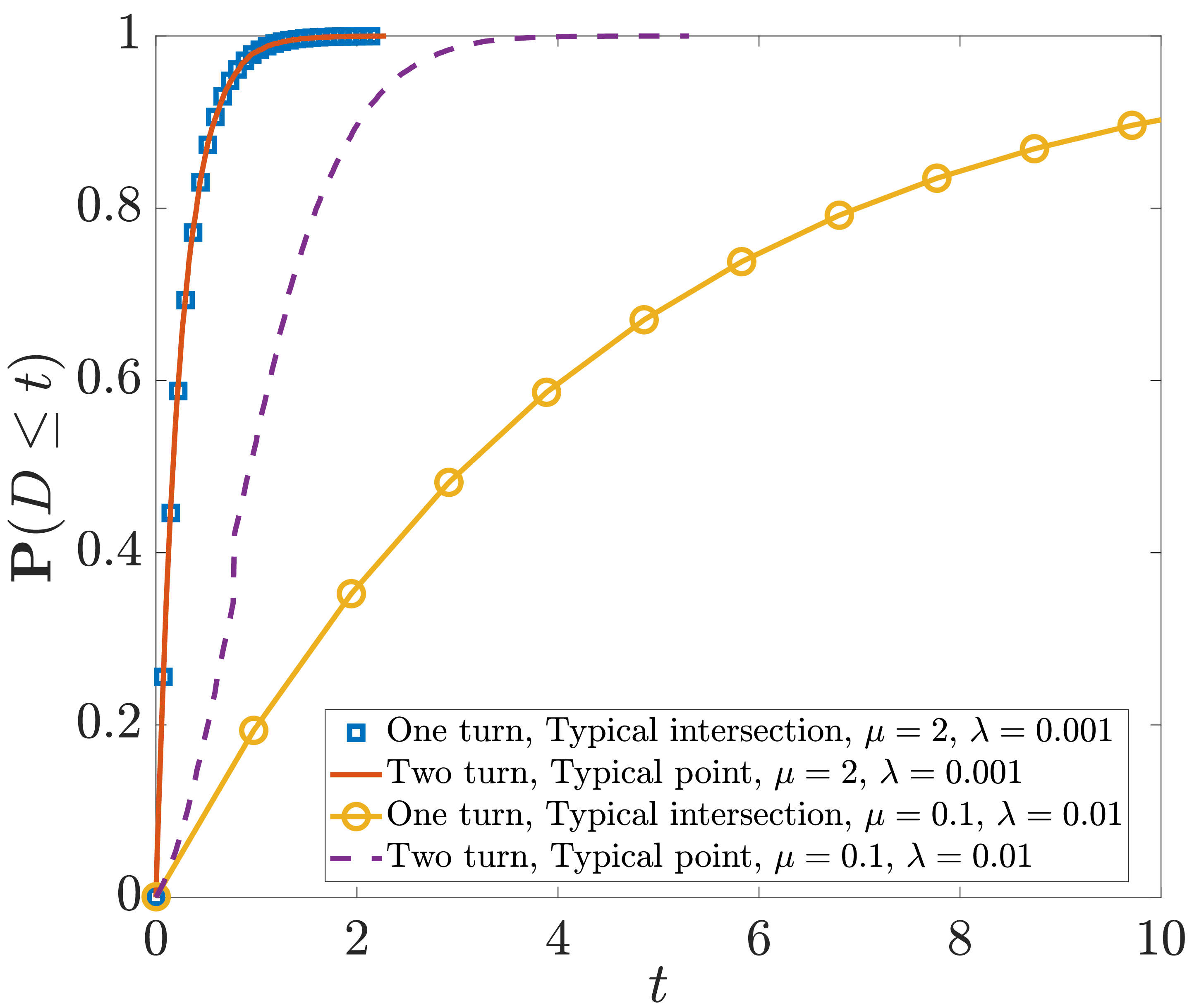
Fig. 8 compares the shortest path length distribution from the typical point and the typical intersection for the single turn case with the same from the typical point for the two turn case. For illustration we have also plotted the analytical bound derived in Theorem 3. Naturally, allowing for two turns statistically brings the nearest point of the PLCP closer. However, Fig. 9 shows that based on the line and point densities, the distance to the nearest point may be same for the two turn case form the typical point and the one turn case from the typical intersection. Indeed, while the former has the benefit of having two starting paths, i.e., along \(L_{\rm x}\) and \(L_{\rm y}\), the later has the advantage of taking two turns, thereby resulting in the same statistics of the shortest path length, especially for high values of \(\mu\) and low values of \(\lambda\). On the contrary, for high \(\lambda\) and/or low \(\mu\), the nearest point is much closer to the typical point if two turns are allowed as compared to the typical intersection in case only a single turn is allowed.
6 Case Study: Quantitative Evaluation in an Urban Ride-Hailing System↩︎
In this section, we quantitatively demonstrate how the analytical results can be directly embedded into the performance evaluation and dimensioning of a transportation system. We explicitly map the theoretical distance distributions to measurable operational metrics, including expected pickup distance and service reliability.
6.1 System Model and Operational Objective↩︎
Consider an urban ride-hailing system operating in a dense downtown region whose road layout is well approximated by a stationary PLP with line intensity \(\lambda\). Vehicles are distributed along each road according to independent one-dimensional PPP with linear intensity \(\mu\), forming the PLCP. We consider a passenger request occurring at the typical intersection and let \(D\) denote the shortest path distance from the request location to the nearest available vehicle. The key operational questions of interest are: what is the expected pickup distance \(\mathbb{E}[D]\); what vehicle density \(\mu\) guarantees a target level of service reliability; and what is the quantitative benefit of allowing additional turns. All three can be answered directly using the derived expressions as discussed below.
6.2 Real-World Data-Driven Parameter Extraction↩︎
However, before proceeding to the numerical analysis, to construct the street network models with realistic parameters, we employ the OSMnx Python library, which facilitates the modeling, analysis, and visualization of street networks derived from
OpenStreetMap data [16]. Leveraging these real-world datasets, we approximate the parameters of the PLP, thereby enabling a statistically robust representation of urban street configurations. Specifically, the street network data are utilized to estimate the PLP intensity parameter \(\lambda_{\rm L}\). For a PLP, the expected total length of line segments within a
given planar region is given by the product of \(\lambda_{\rm L}\) and the area of that region. By considering the geographical region of interest as a disk, we obtain an estimate of the street intensity, \(\hat{\lambda}_{\rm L}\), as \[\begin{align} \hat{\lambda}_{\rm L} = \frac{\pi}{\texttt{street\textunderscore density}},
\end{align}\] where streetdensity denotes the street length density computed using OSMnx. As an illustrative example, the estimated value of \(\hat{\lambda}_{\rm L}\) corresponding to the network
snapshot depicted in Fig. 11 is 0.0052 m\(^{-1}\) and 0.0065 m\(^{-1}\) for Toulouse and Vancouver, respectively.
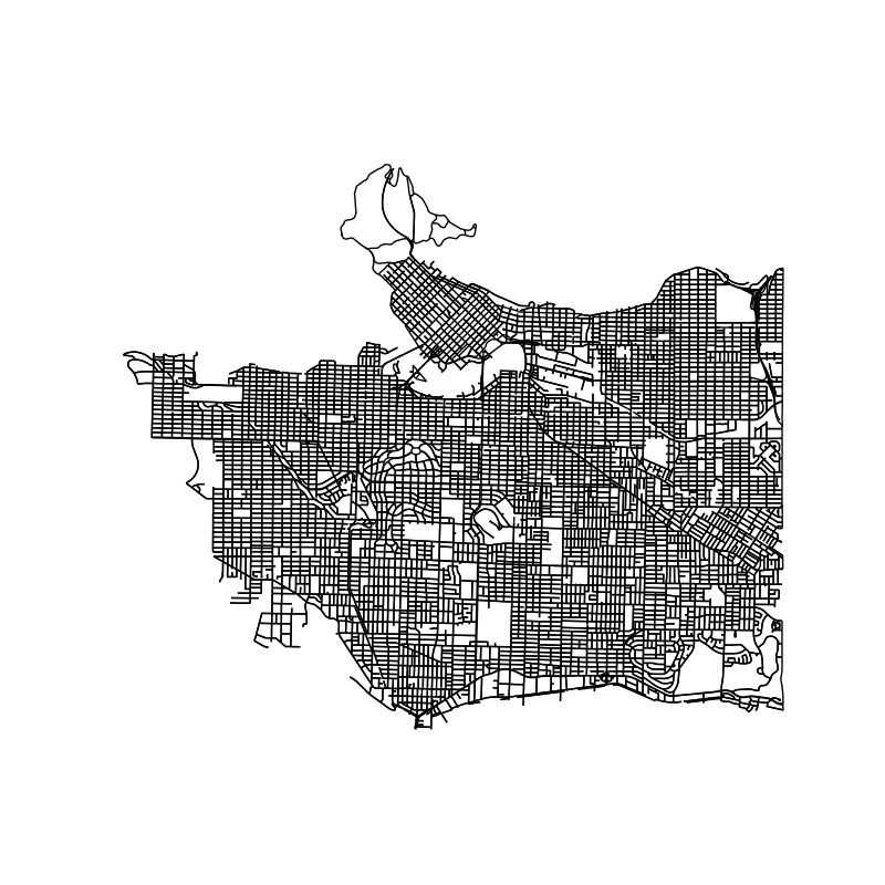
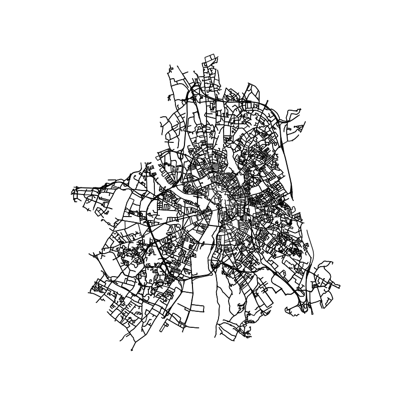
Figure 11: Map (from OSMnx) of different cities considered for determination of a working \(\lambda_L\): (a) Vancouver and (b) Toulouse..
6.3 Expected Pickup Distance↩︎
Given the distribution of the path length, the expected pickup distance is \[\begin{align} \mathbb{E}[D] = \int_{0}^{\infty} \mathbb{P}(D>t)\,{\rm d}t. \label{eq:mean95distance} \end{align}\tag{8}\] Using the exact void probability in Theorem 2, \(\mathbb{P}(D>t) = \exp\!\left(-4\mu t - 2\lambda(2t-\mathcal{T}_x-\mathcal{T}_y) \right)\), substitution into 8 yields a single integral that can be evaluated numerically for any \((\lambda,\mu)\). For example, consider the representative urban parameters \(\lambda = 0.0052 \text{ m}^{-1}\) for Toulouse and \(\mu = 0.02 \text{ m}^{-1},\) corresponding to an average road spacing of 200 m and vehicle spacing of 50 m, numerical evaluation gives \(\mathbb{E}[D_{\text{1-turn}}] \approx 63 \text{ m}.\) On the contrary, using Theorem 1, \(\mathbb{P}(D>t)=\exp\left( -2\mu t -4\lambda t + \frac{2\lambda}{\mu}(1-e^{-2\mu t}) \right),\) which yields \(\mathbb{E}[D_{\text{0-turn}}] \approx 92 \text{ m}\). Thus, we see that allowing a single turn reduces expected pickup distance by approximately \(31\%\) under these parameters. Theorem 3 provides an upper bound on \(\mathbb{P}(D\le t)\) under the two-turn constraint and it enables quantitative comparison with the single-turn case. Using the bound in Theorem 3, we compute \(\mathbb{E}[D_{\text{2-turn}}] \lesssim 58 \text{ m}.\) Compared with the single-turn value of 63 m, the additional reduction is approximately \(8\%\). The first turn yields substantial performance improvement, while the second turn provides diminishing returns. This insight is directly obtained from the analytical expressions and would be difficult to infer from qualitative reasoning alone.
6.4 Service Reliability and Fleet Dimensioning↩︎
Define a service guarantee threshold \(d_0\) (i.e., the maximum acceptable pickup distance). The reliability constraint is \(\mathbb{P}(D \le d_0) \ge \eta,\) for some target probability \(\eta\) (e.g., \(\eta=0.9\)). Using Theorem 2, this becomes \[\begin{align} 1 - \exp\!\left( -4\mu d_0 - 2\lambda(2d_0-\mathcal{T}_x-\mathcal{T}_y) \right) \ge \eta. \label{eq:reliability95constraint} \end{align}\tag{9}\] Solving 9 for \(\mu\) numerically provides the minimum vehicle density required to meet the service guarantee. As an example, in Vancouver, for \(d_0=100\) m and \(\eta=0.9\), numerical inversion yields \(\mu_{\min} \approx 0.015 \text{ m}^{-1},\) corresponding to an average vehicle spacing of approximately 67 m. Thus, the results directly provide fleet sizing guidelines without resorting to Monte Carlo simulations. Furthermore, let \(v\) denote the average vehicle speed. The pickup time is \(T=D/v\) (correspondingly, \(t_0=d_0/v\)). The distance-based service reliability can thus be translated to a time-based service reliability, i.e., \(\mathbb{P}(T \le t_0)\).
6.5 Comparison With Euclidean Planning↩︎
If one incorrectly approximates the PLCP with an equivalent PPP so as to estimate the distance using the Euclidean nearest-neighbor distance with intensity \(\lambda\mu\), the CDF would scale approximately as \(\mathbb{P}(R \le r) = 1-\exp(-\pi \lambda\mu r^2),\) which incorrectly estimates network-constrained distance. We show below analytically that whether the Euclidean approximation over-estimates or underestimates the path-length depends on the system parameters.
Theorem 4. Let \(F_{\mathrm{PPP}}(t) = 1-\exp\!\left( -\pi^{2}\lambda\mu t^{2} \right)\) denote the nearest-neighbor distance distribution in a planar Poisson point process of intensity \(\lambda_{\mathrm{PPP}} = \pi\lambda\mu.\)
Define \[g(t) = \pi^{2}\lambda\mu t^{2} - 2(\mu+\lambda)t + \frac{\lambda}{\mu} \left(1-e^{-2\mu t}\right).\] Then, (i) the crossing points of \(F_1\) and \(F_{\mathrm{PPP}}\) are precisely the roots of \(g\), (ii) The function \(g\) is strictly convex on \([0,\infty)\), and (iii) there exists a unique positive root \(t^\star>0\) satisfying \(g(t^\star)=0.\)
Furthermore, the ordering \[\begin{align} & F_1(t)>F_{\mathrm{PPP}}(t), &0<t<t^\star, \\ &F_1(t)<F_{\mathrm{PPP}}(t), &t>t^\star \end{align}\] holds. Consequently, \(F_1\) and \(F_{\mathrm{PPP}}\) cross exactly once on \((0,\infty)\).
Proof. Since \(x\mapsto 1-e^{-x}\) is strictly increasing on \([0,\infty)\), we have \(F_1(t)=F_{\mathrm{PPP}}(t)\) if and only if \(2(\mu+\lambda)t-\frac{\lambda}{\mu}(1-e^{-2\mu t})=\pi^{2}\lambda\mu t^{2}\), i.e., \(g(t)=0\); hence the crossing points are precisely the roots of \(g\). Note that \(g(0)=0\), \(g'(t)=2\pi^{2}\lambda\mu t-2(\mu+\lambda)+2\lambda e^{-2\mu t}\) and thus \(g'(0)=-2\mu<0\), so \(g(t)<0\) in a neighborhood of \(0\). Moreover, \(g''(t)=2\pi^{2}\lambda\mu-4\lambda\mu e^{-2\mu t}=2\lambda\mu(\pi^{2}-2e^{-2\mu t})\ge 2\lambda\mu(\pi^{2}-2)>0\) since \(0<e^{-2\mu t}\le 1\), so \(g\) is strictly convex on \([0,\infty)\) and \(g'\) is strictly increasing with \(g'(0)<0\) and \(\lim_{t\to\infty}g'(t)=+\infty\). Therefore there exists a unique \(t_m>0\) such that \(g'(t_m)=0\), and this \(t_m\) is the unique global minimizer of \(g\). Since \(g(t_m)<g(0)=0\) while \(\lim_{t\to\infty}g(t)=+\infty\), the Intermediate Value Theorem gives at least one positive root \(t^\star>t_m\) with \(g(t^\star)=0\); by strict convexity and the existing root at \(0\), this \(t^\star\) is unique. Finally, for \(0<t<t^\star\) we have \(g(t)<0\), equivalently \(2(\mu+\lambda)t-\frac{\lambda}{\mu}(1-e^{-2\mu t})<\pi^{2}\lambda\mu t^{2}\), and exponentiating yields \(F_1(t)>F_{\mathrm{PPP}}(t)\); similarly, for \(t>t^\star\) we have \(g(t)>0\) and thus \(F_1(t)<F_{\mathrm{PPP}}(t)\). Hence the two distributions cross exactly once at \(t=t^\star\). ◻
Remark 4. Theorem 4 implies that the one-turn PLCP distance and the matched-intensity PPP distance are not comparable in the sense of first-order stochastic dominance. Consequently, shorter distances are more likely to occur in the PLCP than in the matched-intensity PPP, while longer distances are more likely to occur in the PPP than in the PLCP.
Corollary 3 (Vehicle-density crossing). Fix a threshold distance \(t>0\) and line intensity \(\lambda>0\). If there exists a unique solution \(\mu^\star>0\) of \(2(\mu+\lambda)t-\frac{\lambda}{\mu}\left(1-e^{-2\mu t}\right)=\pi^2\lambda\mu t^2\), then \(F_1(t;\mu)>F_{\mathrm{PPP}}(t;\mu)\) for \(0<\mu<\mu^\star\), whereas \(F_1(t;\mu)<F_{\mathrm{PPP}}(t;\mu)\) for \(\mu>\mu^\star\). Consequently, for the fixed threshold \(t\), the one-turn PLCP and matched-intensity PPP models exhibit a unique crossover as a function of the vehicle density.
6.6 Numerical Results and Discussion↩︎
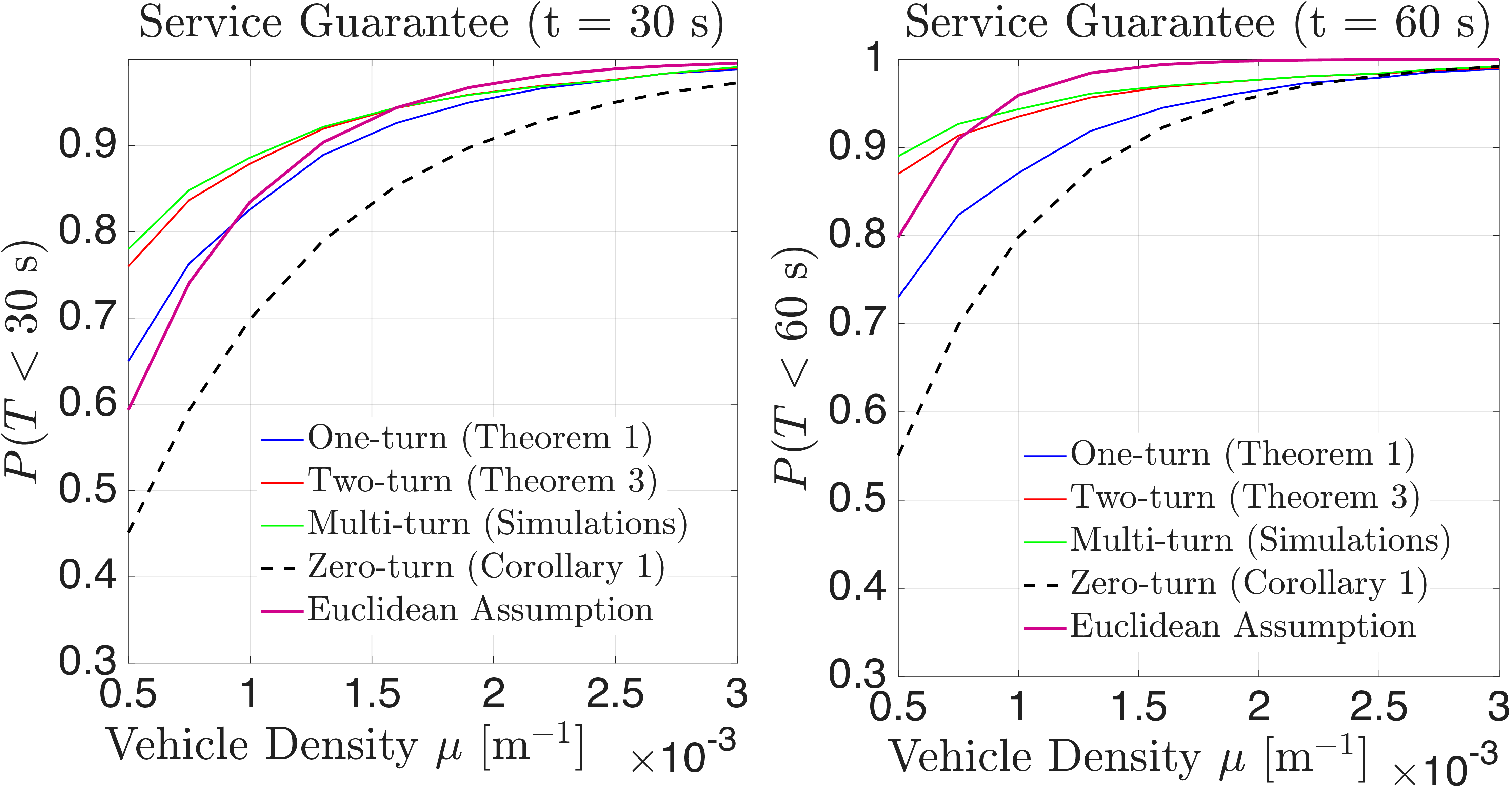
Fig. 10 illustrates the service guarantee \(\mathbb{P}(T<t)\) as a function of the vehicle density \(\mu\) for two latency thresholds: (a) \(t = 30\) s and (b) \(t = 60\) s. For all cases and both latency thresholds, the service guarantee increases monotonically with vehicle density. This behavior is intuitive, as higher density increases the likelihood of encountering a forwarding vehicle within the prescribed deadline, thereby reducing the service time. The zero-turn case consistently provides the lowest service guarantee across the entire density range, while allowing one turn yields a significant improvement. Further gains are observed in the two-turn and multi-turn scenarios, albeit diminishing in the difference, confirming that additional routing flexibility enhances spatial connectivity and improves delay performance marginally.
This suggests that most of the achievable connectivity benefits are captured within two turns. Comparing Figs. 2(a) and 2(b), relaxing the deadline from \(30\) s to \(60\) s shifts all curves upward, with the improvement being more pronounced in the sparse regime where additional time compensates for limited vehicle availability. It is interesting to note that the Euclidean distance assumption crosses the multi-turn plot for a given density consistent with the findings of Corollary 3.
This case study demonstrates that the closed-form expressions in Theorems 1 and 2 enable direct computation of expected pickup distance and reliability, that the bound in Theorem 3 quantifies the marginal value of additional turning flexibility, that fleet sizing and service guarantees can be analytically dimensioned as explicit functions of \((\lambda,\mu)\), and that Euclidean approximations introduce significant structural bias in transportation planning. Importantly, every quantitative metric above is obtained by direct substitution of the derived distance distributions into operational performance formulas. Hence, the proposed stochastic-geometry framework serves not only as a structural characterization tool but as a practical analytical engine for transportation system design.
We stress that from a driving perspective, the one-turn and two-turn shortest-path distributions studied in this paper are not intended to model general navigation based routing with an unrestricted number of turns. Rather, they provide analytically tractable accessibility benchmarks that quantify geometry-induced detours in Poisson-line street networks and are especially relevant for short-range/last-mile accessibility and limited-maneuver routing scenarios. The two-turn analysis represents the first extension beyond single-turn routing and serves as a stepping stone for future extensions to multi-turn routing via numerical methods. It is also interesting to note that the multi-turn option matters most when the driver is in a dense setting with many intersections. There, wrong turns have limited cost because the driver can quickly correct them, so precise path-distance characterization is unnecessary. In contrast, on highways, wrong turns can greatly increase path distance. These low-intersection settings make single- and two-turn characterizations useful.
7 Other Applications↩︎
7.1 Near-Field Broadcasting of Basic Safety Messages Leveraging RIS↩︎
In RF communications, based on electromagnetic principles, the total gain of the cascaded channel (transmitter-RIS-receiver) is approximately the product of the gains from these two sub-channels and the reflection coefficient of the RIS element, characterizing it as a multiplicative channel. In contrast, the channel reflected by an ORIS, especially in the near-field and very near-field regime, behaves as an additive channel [17], [18]. This behavior is also observed in the near-field broadcasting configuration of RISs even for RF communications [19]. In such near-field transmission, the reflected signal can thus be considered as emanating directly from a virtual transmitter, which is symmetrically positioned relative to the actual transmitter across the plane of the RIS reflecting element.
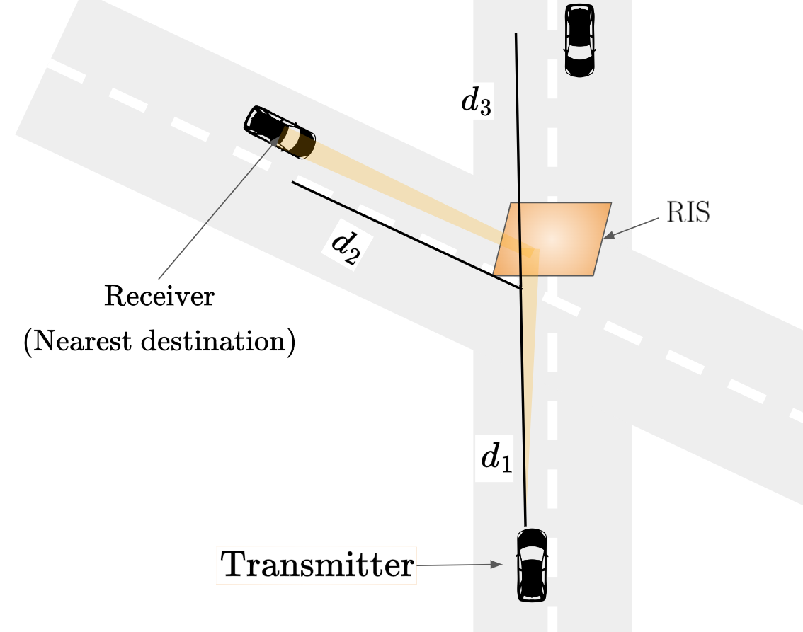
Accordingly, consider the V2V communication system shown in Fig. 12 where the vehicles intend to transmit BSMs to neighboring vehicles as they approach street intersections. The vehicles employ a network-configured PC5 side-link to communicate [20]. Assume that RISs are deployed on the street intersections so that the vehicle on intersecting streets can communication with each other. Considering the size of the RIS to be large as compared to the transmitting distance, the transmitter can be assume to be in the near-field of the RIS. For the transmitter, the nearest vehicle (in terms of the path length) may either be on the same street at a distance \(d_1 + d_3\) from the transmitter (as illustrated in the figure), or in the intersecting street at a path length \(d_1 + d_2\), connected via the RIS. In case the transmitter leverages the RIS to communicate with the receiver located on the intersecting street, the received signal power in the near-field broadcasting regime is approximated as [19] \[\begin{align} P_{ri} \approx \frac{G_t G_r \lambda^2 A^2}{16 \pi^2 (d_1 + d_i)^2} P_t; \quad i \in \{2,3\}, \end{align}\] where \(G_t, G_r,\) and \(P_t\) are respectively the transmitter gain, receiver gain, and the transmit power. The carrier wavelength is \(\lambda\) and \(A\) is the area of the RIS board. Based on the distances of other vehicles, the nearest receiver corresponds to either \(i \in \{2,3\}\). Let us assume that the receiver is able to decode the BSM packets if the received SNR is higher than a threshold \(\gamma\). Naturally, for a noise power \(N_0\), the probability that the nearest vehicle to the transmitter successfully decodes the BSM packet is evaluated as \[\begin{align} \mathbb{P}\left(\max_{i}\{P_r\} \geq \gamma\right) &\approx \mathbb{P}\left(\min_i\{d_1 + d_i\} \leq \left(\frac{16 \pi^2\gamma N_0}{G_t G_r \lambda^2 A^2}\right)^{\frac{1}{2}}\right) \nonumber \\ &=F_D\left(\left(\frac{16 \pi^2\gamma N_0}{G_t G_r \lambda^2 A^2}\right)^{\frac{1}{2}}\right), \end{align}\] which is evaluated using ?? .
7.2 Bound for Far-Field Communications↩︎
The shortest path distribution can be used to derive bound on the far-field communication. In particular, the maximum far-field received power with optimized phase responses and no misalignment is given by [19] \[P_{\text{F}} = \frac{G_t G_r G M^2 N^2 d_x d_y \lambda^2 A^2}{64 \pi^3 d_1^2 d_2^2} P_t,\] where \(d_x\) and \(d_y\) represent the size of a unit cell along the two dimensions of a square RIS. \(M\) and \(N\) are respectively the number of RIS elements along the two dimensions. Consequently, \[\begin{align} &\mathbb{P}\left(P_{\text{F}} \geq \gamma \right) = \mathbb{P}\left(\frac{G_t G_r G M^2 N^2 d_x d_y \lambda^2 A^2}{64 \pi^3 d_1^2 d_2^2} P_t \geq \gamma\right) \nonumber \\ &=\mathbb{P}\left(d_1d_2 \leq \sqrt{\frac{64 \pi^3}{G_t G_r G M^2 N^2 d_x d_y \lambda^2 A^2}}\right) \nonumber \\ &\overset{(a)}{\geq} \mathbb{P}\left(d_1 + d_2 \leq 2\left({\frac{64 \pi^3}{G_t G_r G M^2 N^2 d_x d_y \lambda^2 A^2}}\right)^{\frac{1}{4}}\right) \nonumber \\ &= F_D\left(2\left({\frac{64 \pi^3}{G_t G_r G M^2 N^2 d_x d_y \lambda^2 A^2}}\right)^{\frac{1}{4}}\right), \nonumber \end{align}\] where the step \((a)\) is from the inequality that the arithmetic mean of \(d_1\) and \(d_2\) is greater than the geometric mean.
The V2V application above is an illustrative example of how the derived shortest-path distributions can be used in performance analysis of standardized V2V systems. The considered sidelink communication follows the 3GPP PC5 interface for direct V2V (3GPP TS 23.287, TS 36.300, TS 36.321 for LTE-V2X, and TS 38.300, TS 38.321, TS 38.331 for NR-V2X). Basic safety messages (BSMs) are defined by SAE J2735 and transmitted using IEEE 802.11p/IEEE 1609 WAVE or their cellular V2X counterparts. The proposed shortest-path framework does not change any PHY, MAC, resource allocation, or packet scheduling mechanisms in these standards. Instead, it statistically characterizes the path lengths between communicating vehicles, which can then be mapped to received power, SNR, packet delivery ratio, and latency in standard-compliant V2V systems.
8 Conclusion and Open Questions↩︎
We characterized street-constrained (\(\ell_1\)) nearest-neighbor distances in the PLCP by deriving exact one-turn shortest path length distributions from both the typical PLCP point and the typical PLP intersection. For the intersection case, we additionally developed analytically tractable upper and lower bounds that clarify how the line density \(\lambda\) and the linear point intensity \(\mu\) shape the distribution. Allowing two turns from the typical point, we obtained a computable upper bound via a feasible-set shrinking approach and identified regimes in which it is tight. The analysis also reveals parameter ranges where a one-turn path from a typical intersection can be shorter than a two-turn path from a typical point, highlighting nontrivial tradeoffs between origin selection, routing flexibility, and the pair \((\lambda,\mu)\).
Several questions remain open. Most prominently, an exact characterization of the shortest path length distribution without restricting the number of turns is still unresolved. Related open directions include tighter or exact results for multi-turn routing, connectivity/percolation properties of the induced street-constrained graph, and extensions to anisotropic line processes and nonhomogeneous deployments that better reflect real cities.
References↩︎
G. Ghatak is with Department of Electrical Engineering, IIT Delhi, Hauz Khas, India 110016. Email: gghatak@ee.iitd.ac.in. S. K. Jhawar is with the DYOGENE team, INRIA Paris, France. Email: sanjoy-kumar.jhawar@inria.fr. M. Haenggi is with the Department of Electrical Engineering, University of Notre Dame, Notre Dame, IN 46556 USA (e-mail: mhaenggi@nd.edu).↩︎