Abstract
We propose a novel method for estimating nonseparable selection models. We show that, for a given selection function and under suitable contraction conditions, the potential outcome distributions are nonparametrically identified from the selected outcome distributions and can be recovered using a simple iterative algorithm based on a contraction mapping. This result enables a full-information approach to estimating selection models without imposing parametric or separability assumptions on the outcome equation. We propose a two-step estimation strategy for the potential outcome distributions and the parameters of the selection function and establish the consistency and asymptotic normality of the resulting estimators. Monte Carlo simulations demonstrate that our approach performs well in finite samples. The method is applicable to a wide range of empirical settings, including consumer demand models with only transaction prices, auctions with stochastic winning rules and incomplete bid data, and Roy-type models with data on accepted wages.
Keywords: Sample Selection, Nonseparable Models, Functional Contraction, Potential Outcome Distribution, Semiparametric Estimation, Demand Estimation, Auction, Roy Models.
JEL Codes: C14, C24, C51, L11, D44, J31.
1 Introduction↩︎
Sample selection issues arise in many empirical settings. In consumer demand studies, researchers often observe only the transaction prices of chosen products [1]–[7]. In auctions, available data may consist solely of the winning bids [8]–[11]. In labor economics, wage data are typically observed only for individuals who choose to work [12], [13], and in the Roy model [14], earnings within an occupation are observed only for those who self-select into that sector.
Observing only a selected sample of outcomes—such as prices, bids, or wages—poses significant challenges for estimating two key elements. First is the selection function, which specifies how agents choose among alternatives, for example, through a consumer demand system, an auction’s winning rule, or a labor force participation decision. Second is the distribution of outcomes prior to selection, often referred to as “potential outcomes" in the literature. Flexibly estimating potential outcome distributions is crucial in many empirical contexts, such as analyzing price distributions to understand firms’ pricing strategies and wage distributions to examine inequality.
Our paper proposes a new approach to estimating nonseparable selection models by exploiting a previously unrecognized one-to-one mapping between the outcome distributions before and after selection. Our key contribution is a constructive identification result showing that, for a given selection function and under suitable contraction conditions, the potential outcome distributions are nonparametrically identified from the selected outcome distributions and can be recovered using a simple iterative algorithm. Consequently, the remaining object to be estimated is the selection function, which can be recovered from observed choice patterns. Our method enables a full-information approach to estimating selection models without imposing parametric or separability assumptions on the outcome equation.
Formally, we consider a discrete choice problem in which each alternative is associated with a potential outcome distribution. A selection function maps a vector of realized potential outcomes to a probability distribution over the alternatives. For example, in the consumer demand setting, each alternative represents a product, and the potential outcome is the offered price, with the selection function micro-founded by the consumer’s utility maximization problem. We allow the outcome equations to be fully nonparametric with nonseparable error terms and to vary flexibly across different alternatives. We assume that potential outcomes across alternatives are independent conditional on observable and unobservable characteristics, which allows for correlation across outcomes when conditioning only on observables. Our framework also permits the unobservable component in the outcome equation to enter directly into agents’ preferences over alternatives, thereby capturing selection on unobservables.
We analyze how the selection model maps the potential outcome distributions to the distributions of selected outcomes and seek to invert the mapping. The key insight of our approach is that, given the selection model and potential outcome distributions across all alternatives, we can derive the likelihood of an outcome being selected at each price. Conversely, if this selection likelihood were known, we could recover the potential outcome distributions from the selected outcome distributions using Bayes’ rule. This two-way relationship characterizes a fixed-point problem.
Building on this intuition, we construct an operator whose fixed point is the potential outcome distributions and establish sufficient conditions for it to be a functional contraction (Theorems 1 and 2). Our results imply that, given the selection function and the distributions of selected outcomes, we can nonparametrically identify the potential outcome distributions under the contraction condition. Importantly, the contraction condition is automatically satisfied in binary choice models. Moreover, this identification result is constructive: starting with any initial guess for the potential outcome distributions, we iteratively apply the operator. This process converges to the potential outcome distributions associated with the selection function.
We then embed this identification result into a two-step estimation strategy for the unobserved potential outcome distributions and the parameters of the selection function. In the first step, we estimate the selected outcome distribution conditional on both observable and unobservable covariates using the instrumental variable approach from the nonclassical measurement error literature [15], [16]. In the second step, we propose a nested fixed-point algorithm to estimate the parameters of the selection function: in the inner loop, for any candidate selection function, we recover the potential outcome distributions by iterating the operator, while in the outer loop we search for the parameter values that maximize the likelihood of the observed choice patterns. The potential outcome distributions are then obtained by reapplying the fixed-point algorithm at the estimated parameters of the selection function.
We establish the consistency and asymptotic normality of the proposed estimators in Theorems 3 and 4 under suitable regularity conditions. To examine their finite sample properties, we conduct Monte Carlo simulations across various designs of the outcome equation. Our results show that the biases in our estimators are generally small, and the standard deviation decreases as the sample size increases across all simulation designs. Our nonparametric estimation of the potential outcome distributions outperforms the classic Heckman parametric two-step approach and the quantile selection model of [17] with linear quantile functions and a Gaussian copula, particularly when the outcome equation contains nonseparable error terms.
In [7], we apply our method to estimate consumer demand for auto insurance products when only transaction prices are observed. We nonparametrically estimate the offered price distribution for each insurance company and allow these distributions to vary fully flexibly across firms. The substantial heterogeneity in the recovered price distributions reflects differences in firms’ information technologies and cost structures, which are key primitives we estimate through a supply-side competition model. We omit the details of this application here and refer readers to [7] for the full empirical setup and results.
1.0.0.1 Related Literature
Our paper contributes to the extensive theoretical literature on sample selection models. An early solution to sample selection bias is full information maximum likelihood (FIML) estimation based on parametric assumptions, as in [13] and [18] ([18], [19]). More commonly employed methods for sample selection models are the two-step control function approach pioneered by [20] ([20], [21]). A substantial body of theoretical work has been developed to relax the distributional assumptions in the two stages of the estimation procedure [22]–[29]. For a comprehensive survey of semiparametric two-step estimation methods for selection models, see [30].
Our approach provides an alternative framework that differs from existing methods along several dimensions. First, we allow the outcome equation to be nonparametric and nonseparable in the error terms, and we exploit the full information in the selected outcome distribution to recover the entire distribution of potential outcomes. [26] and [28] use control function approaches to correct for sample selection in nonseparable models with binary and censored selection rules, respectively, and they focus on identifying certain global and local parameters of the outcome distribution.
Second, our method accommodates fully heterogeneous effects of covariates on outcomes. By contrast, many existing approaches that estimate conditional mean models restrict covariates to affecting only the location of the outcome distribution. Notable exceptions include [17], who develop a sample-selection correction for quantile regression by modeling the copula of the error terms in the outcome and selection equations, and [29], who propose a semiparametric generalization of the Heckman selection model that allows for rich forms of heterogeneity in the effects of covariates on both outcomes and selection.
Third, our approach does not require the conventional exclusion restriction used in many sample selection models, namely a variable that shifts the choice probability without directly affecting outcomes. Such variables are central to identification in many two-step procedures and may not always be readily available in practice (see [30] and [31] for further discussion). Furthermore, our method does not rely on identification-at-infinity arguments.2
Instead, we assume that the potential outcomes are conditionally independent given the observed and unobserved characteristics, and our method relies on instruments satisfying the conditional independence requirements of the nonclassical measurement-error literature, as in [15] and [16], to estimate the selected outcome distributions conditional on the unobservable in the first step. These instruments serve a different role from the exclusion restrictions commonly used in sample selection models. Neither identifying strategy is uniformly weaker than the other; rather, they represent alternative sources of identifying variation that may be more or less plausible depending on the application.
Estimation of the selection function in our model is closely related to the demand estimation literature following the seminal work of [35] and [36]. In particular, observed choice patterns play the same role as market shares in recovering consumer preference parameters. Our method addresses the problem of missing full price menu that arises in many demand estimation contexts [1]–[7], an issue that is especially relevant in the presence of price discrimination or personalized pricing.3
At a broader conceptual level, our reliance on the structural restrictions implied by the selection model resonates with the nonparametric identification literature on auction models with missing bids and competing risks models [8]–[10], [37].4 In these models, the selection rule is deterministic (e.g., the highest bidder wins), which allows order-statistic arguments to be applied. In contrast, our selection model assigns a probability distribution over alternatives and is therefore closer in spirit to multi-attribute auction environments [38]. Because selection is probabilistic rather than determined by an extremal outcome, classical order-statistic techniques are not applicable. Instead, our identification strategy relies on a fixed-point characterization of the selection process. Moreover, our framework can flexibly accommodate asymmetries across alternatives, whereas bidder asymmetries are known to pose significant challenges in auction models (see the discussion in the handbook chapter by [39]).
1.0.0.2 Outline
The rest of the paper is organized as follows. Section 2 formally introduces our model and presents the main theoretical results. In Section 3, we describe our estimation strategy and establish the asymptotic properties of the estimators. Section 4 reports results from our Monte Carlo simulations, and Section 5 discusses the empirical application in [7]. Section 6 concludes. All proofs are collected in the appendix.
2 Model and Main Results↩︎
In this section, all analyses are conditional on a vector of characteristics \((x, x^\ast)\), where \(x\) denotes observables and \(x^\ast\) denotes unobservables. The structure of the model and the main theoretical results do not depend on whether the conditioning set includes unobserved components, although the presence of unobservables introduces additional challenges for estimation, which we address in Section 3. Because all results in this section are stated conditional on \((x, x^\ast)\), we omit these variables from the notation to simplify exposition.
Consider a discrete choice problem. There is a finite set of alternatives \(\mathcal{J}=\{1, \ldots, J\}\). Each alternative is associated with a price distribution. Let \(G_j \in \Delta ([\underline p_j, \overline{p}_j])\) denote the price distribution associated with alternative \(j\), where \(\Delta (A)\) denotes the set of all probability measures over a set \(A\subset \mathbb{R}\). The collection of \(G_j\) is denoted by \(G=\prod_{j\in\mathcal{J}} G_j\). We refer to \(G\) as the offered price distribution.
We assume that the offered prices \(p_j\sim G_j\) are independently distributed across alternatives, conditional on \(x\) and \(x^\ast\). This assumption allows prices across alternatives to be correlated conditional on observables. For example, if \(x^\ast\) captures a worker’s unobserved productivity, wage offers from different firms may appear correlated when conditioning only on observable characteristics. However, the assumption imposes a more restrictive dependence structure: any residual correlation across prices must be mediated by \(x^\ast\), rather than allowing prices to be arbitrarily correlated conditional on observables. Nevertheless, \(x^\ast\) is not restricted to be one-dimensional and may instead represent a high-dimensional vector of latent characteristics. As the conditioning information becomes richer, more of the dependence across alternatives is captured by the observed and latent characteristics, leaving less residual dependence to be ruled out by the conditional independence assumption.
A selection function is denoted by \(f=(f_1,f_2,\ldots,f_J)\) where \(f_j\) maps prices \(\boldsymbol{p}=(p_1, \ldots, p_J)\) to the probability of selecting alternative \(j \in \mathcal{J}\). We assume that \(f_j\) is continuous on the compact price support and strictly positive: \[f_j:\prod_j[\underline p_j,\overline{p}_j]\to(0,1],\] with \(\sum_{j\in\mathcal{J}} f_j\le 1\). The inequality allows for the case with an outside option.
The strict positivity assumption ensures that every price realization has a positive probability of generating an observed choice and therefore can, in principle, be observed in the data. To see why this is important, suppose instead that there exists an interval \(A \subset [\underline{p}_j, \overline{p}_j]\) such that whenever \(p_j \in A\), the probability of choosing alternative \(j\) is zero. Then prices in \(A\) are effectively censored from the data; that is, the data contain no information about the frequency with which such prices are offered. As a result, \(G_j\) cannot be identified on \(A\) without imposing additional restrictions.5
The selection function \(f\) is taken as a primitive of our framework. Nevertheless, it can be microfounded through a standard utility-maximization problem. Under particular assumptions on the distribution of utility shocks, familiar discrete choice models such as the multinomial logit and probit arise as special cases. We also want to emphasize that the selection function \(f\) can freely depend on observable and unobservable characteristics \((x, x^\ast)\). This flexibility allows the model to capture dependence between the potential outcome distribution and the selection mechanism. For example, unobserved productivity may simultaneously influence wage offers and labor-force participation decisions, thereby generating endogenous selection.
The offered price distribution (or potential outcome distribution) \(G_j\) is generally not directly observed in the data, yet it is often the primary object of interest. Instead, data typically reveal only the selected (or accepted) outcome distribution. For example, researchers may observe the distribution of transacted prices or accepted wage offers, but not the distribution of all offered prices or wage offers. Let \(\tilde{G}_j\in \Delta ([\underline p_j, \overline{p}_j])\) represent the price distribution of alternative \(j\) conditional on \(j\) being selected. Similarly, \(\tilde{G}=\prod_{j\in\mathcal{J}} \tilde{G}_j\) denotes the collection of selected outcome distributions across all alternatives.
In the remainder of this section, we establish identification of the potential outcome distributions \(G\) from the selected outcome distributions \(\tilde{G}\), holding the selection function \(f\) fixed. We then turn in Section 3 to the empirically relevant case in which \(f\) is specified up to a finite-dimensional parameter vector that is estimated from observed choice behavior.
2.1 A Fixed-Point Characterization of Potential Outcome Distributions↩︎
We begin with a density-based formulation that highlights the main ideas most transparently. Throughout Section 2.1, we assume that all relevant distributions admit densities with full support and use lower-case letters to denote densities corresponding to probability measures denoted by upper-case letters. In particular, let \(g_j\) and \(\tilde{g}_j\) denote the densities of the probability measures \(G_j\) and \(\tilde{G}_j\), respectively. Similarly, let \(g=\prod_{j\in\mathcal{J}} g_j\) and \(\tilde{g}=\prod_{j\in\mathcal{J}} \tilde{g}_j\) denote the collections of potential and selected outcome densities across all alternatives, respectively. A measure-theoretic formulation accommodating general probability measures, including discrete distributions, continuous distributions, and arbitrary mixtures thereof, is provided in Section 2.2.
The density of selected outcomes \(\tilde{g}_j\) can be derived from the density of potential outcomes \(g_j\) using Bayes’ rule: \[\label{eq:32expost} \tilde{g}_j(p_j)\propto Pr_j(p_j;g) g_j(p_j), \text{ for all } j.\tag{1}\] In Equation (1 ), \(Pr_j(p_j;g)\) represents the probability of selecting alternative \(j\) conditional on \(p_j\) and is given by \[\begin{align} \label{eq:choice95prob} Pr_j(p_j;g)=\int_{\boldsymbol{p}_{-j}}f_j(p_j, \boldsymbol{p}_{-j})\prod_{k\neq j}g_k(p_k)d\boldsymbol{p}_{-j}, \end{align}\tag{2}\] where \(\boldsymbol{p}_{-j}=(p_1, \ldots, p_{j-1}, p_{j+1}, \ldots, p_J)\) denotes the vector of prices excluding \(j\)’s price. Because we assume that prices are independently distributed across alternatives conditional on \((x,x^\ast)\), the joint distribution of \(\boldsymbol{p}_{-j}\) factors into the product of the marginal densities, \(\prod_{k\ne j} g_k(p_k)\).
Collecting Equations 1 and 2 across all alternatives \(j \in \mathcal{J}\) defines a forward mapping from the potential outcome distributions to the selected outcome distributions, where the selection mechanism is governed by the selection function \(f\) through the conditional choice probabilities. Our objective, however, is the inverse: to recover the unobserved potential outcome distributions \(g\) from the observed selected outcome distributions \(\tilde{g}\).
Whether such recovery is possible depends critically on the information contained in the observed data. In this regard, the conditional independence assumption plays a key role in identification. Because the data reveal only the price of the selected alternative, they contain no direct information about the dependence structure of prices across alternatives. As a result, any correlation among competing alternatives is generally unidentifiable.6 For example, if prices tend to move together across alternatives, this dependence would not be detectable from the observed data. The conditional independence assumption circumvents this problem by restricting the joint distribution of prices to be determined by the marginal distributions. As a result, for a given selection function, the system defined by Equations 1 and 2 contains as many unknown objects as identifying restrictions: both \(g\) and \(\tilde{g}\) consist of \(J\) densities. Even so, identification remains challenging because it requires recovering a collection of infinite-dimensional objects from a nonlinear system of equations.
To address this challenge, we now derive an inversion of the forward mapping defined by Equations 1 and 2 . In particular, dividing both sides of Equation 1 by the selection probability \(Pr_j(p_j;g)\) yields \[\label{eq:inversion} g_j(p_j)\propto \tilde{g}_j(p_j)/Pr_j(p_j;g), \text{ for all } j .\tag{3}\] We illustrate this inversion process using the simulated example in Figure 1. The red solid line plots the selected price density for an alternative. Dividing this density by the probability that the alternative is chosen at each price, \(Pr_j(p_j;g)\), yields the unnormalized offered price density shown by the blue dashed line. The gap between these two densities captures the selection mechanism: when a lower price is offered, agents are more likely to accept it, whereas higher prices make them more likely to choose other alternatives. The offered price distribution shown by the blue solid line is then obtained after normalization.
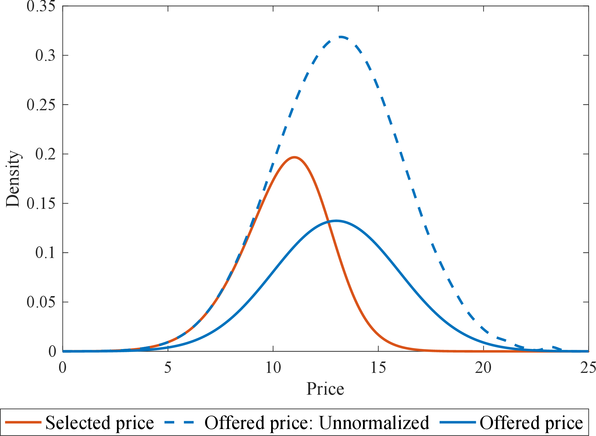
Equation (3 ) plays a central role in our analysis. Note that if the selection probability \(Pr_j(\cdot;g)\)—that is, the probability of selecting product \(j\) conditional on its offered price—were known, then recovering the offered price distribution from Equation (3 ) would be straightforward. However, \(Pr_j(\cdot;g)\) is not known, because it depends on the offered price distribution \(g\), which we seek to recover. A tentative solution is to start with a conjecture \(\psi\) for the offered price distribution and use it to compute the implied selection probability \(Pr_j(\cdot;\psi)\). Equation (3 ) then delivers an updated conjecture of the offered price distribution. This procedure, which maps a conjectured offered price distribution into its updated version, defines an operator \(T\colon \prod_j \Delta([\underline p_j, \overline{p}_j])\to \prod_j \Delta([\underline p_j, \overline{p}_j])\) as follows. \[\label{eq:operator} (T\psi)_j(p_j)=\frac{ \tilde{g}_j(p_j)/Pr_j(p_j;\psi) }{ \int_{\underline p_j}^{\overline{p}_j} \tilde{g}_j(p)/Pr_j(p;\psi)dp }, \text{ for all } j.\tag{4}\] where \(\psi=(\psi_1,\psi_2,\ldots,\psi_J)\in \prod_j \Delta([\underline p_j, \overline{p}_j])\). The denominator is the normalizing constant that ensures \((T\psi)_j\) integrates to one.
Importantly, if the conjecture \(\psi\) is correct, i.e., \(\psi=g\), then the selection probability \(Pr_j(\cdot;\psi)\) is correct, ensuring that the updated conjecture \(T\psi\) also equals \(g\). Thus, the offered price distribution \(g\) is a fixed point of the operator \(T\).
The operator \(T\) is a contraction if there exists some real number \(0\leq \rho<1\) such that for all \(\psi, \phi\in \prod_j \Delta([\underline p_j, \overline{p}_j])\), \[\label{eq:contraction32definition} D(T\psi, T\phi)\leq \rho D(\psi, \phi),\tag{5}\] given some metric \(D\).7 We now introduce a suitable metric.
2.1.0.1 Hilbert’s Projective Metric
For two densities \(\psi_j,\phi_j \in \Delta([\underline{p}_j,\overline{p}_j])\), we measure their distance using Hilbert’s projective metric. If \(\psi_j\) and \(\phi_j\) are strictly positive on the same support, \[\label{eq:hilbert} d_H(\psi_j,\phi_j) = \ln \bigg(\frac{ \operatorname*{sup}_{p\in[\underline{p}_j,\overline{p}_j]} \frac{\psi_j(p)}{\phi_j(p)}}{\operatorname*{inf}_{p\in[\underline{p}_j,\overline{p}_j]} \frac{\psi_j(p)}{\phi_j(p)}} \bigg ),\tag{6}\] otherwise set \(d_H(\psi_j,\phi_j)=+\infty\).
The choice of this metric is deliberate and closely tailored to the structure of the operator \(T\). In particular, the usefulness of Hilbert’s projective metric in our setting comes from its invariance to positive rescaling. Since the operator \(T\) updates each density by reweighting \(\tilde{g}_j\) by the reciprocal of selection probability \(Pr_j(\cdot;\psi)\) and then renormalizing, both the common factor \(\tilde{g}_j\) and the normalizing constants cancel out when computing the projective distance. Therefore, for any two conjectured densities \(\psi\) and \(\phi\), \[\begin{align} d_H((T\psi)_j,(T\phi)_j) & = \ln \bigg(\frac{ \operatorname*{sup}_{p\in[\underline{p}_j,\overline{p}_j]} \frac{(T\psi)_j(p)}{(T\phi)_j(p)}}{\operatorname*{inf}_{p\in[\underline{p}_j,\overline{p}_j]} \frac{(T\psi)_j(p)}{(T\phi)_j(p)}} \bigg ) \\ & = \ln \bigg( \frac{\operatorname*{sup}_{p\in[\underline{p}_j,\overline{p}_j]} \frac{ \tilde{g}_j(p)/Pr_j(p;\psi) }{ \text{norm.\;const.\;for \psi} } \frac{\text{norm.\;const.\;for \phi} }{ \tilde{g}_j(p)/Pr_j(p;\phi) } }{ \operatorname*{inf}_{p\in[\underline{p}_j,\overline{p}_j]} \frac{ \tilde{g}_j(p)/Pr_j(p;\psi) }{ \text{norm.\;const.\;for \psi} } \frac{\text{norm.\;const.\;for \phi} }{ \tilde{g}_j(p)/Pr_j(p;\phi) } } \bigg) \\ & =\ln \bigg(\frac{ \operatorname*{sup}_{p\in[\underline{p}_j,\overline{p}_j]} \frac{Pr_j(p;\phi)}{Pr_j(p;\psi)}}{\operatorname*{inf}_{p\in[\underline{p}_j,\overline{p}_j]} \frac{Pr_j(p;\phi)}{Pr_j(p;\psi)}} \bigg ) = d_H(Pr_j(\cdot;\phi),Pr_j(\cdot;\psi)). \end{align}\] This equation reveals an important isometry: measuring the distance between \((T\psi)_j\) and \((T\phi)_j\) is equivalent to measuring the distance between the corresponding selection probabilities under Hilbert’s projective metric. Consequently, the contraction properties of the operator \(T\) can be characterized by studying how perturbations in the conjectured densities affect the implied choice probabilities.
2.2 General Probability Measure Formulation↩︎
The density formulation in Section 2.1 is useful for illustrating the key ideas but is not essential for the results. We now present the corresponding measure-theoretic formulation for arbitrary probability measures and adopt this framework for the rest of the paper.
As before, the selected outcome distribution \(\tilde{G}_j\) can be derived from the potential outcome distribution \(G_j\) via Bayes’ rule. For any Borel set \(A\subseteq[\underline p_j,\overline{p}_j]\), the counterpart of Equation 1 for general probability measures is: \[\label{eq:32expost95app} \tilde{G}_j(A) = \frac{ \int_A Pr_j(p_j;G)\,dG_j(p_j) }{ \int_{\underline p_j}^{\overline{p}_j} Pr_j(p_j;G)\,dG_j(p_j) }, \text{ for all }j,\tag{7}\] where \[\label{eq:choice95prob95app} Pr_j(p_j;G)=\int_{\boldsymbol{p}_{-j}}f_j(p_j, \boldsymbol{p}_{-j})\prod_{k\neq j}dG_k(p_k).\tag{8}\] Equation 7 defines a mapping \(F\colon \prod_j \Delta([\underline p_j, \overline{p}_j])\to \prod_j \Delta([\underline p_j, \overline{p}_j])\) that maps the potential outcome distribution \(G\) to the selected outcome distribution \(\tilde{G}\).
The inversion argument developed in the density-based framework extends directly to the present setting. In particular, the counterpart of Equation 3 is \[\label{eq:inversion95app} G_j(A) = \frac{ \int_A d\tilde{G}_j(p_j)/Pr_j(p_j;G) }{ \int_{\underline p_j}^{\overline{p}_j} d\tilde{G}_j(p_j)/Pr_j(p_j;G) }, \text{ for all }j.\tag{9}\] Equation 9 defines an operator \(T\colon \prod_j \Delta([\underline p_j, \overline{p}_j])\to \prod_j \Delta([\underline p_j, \overline{p}_j])\) as follows. \[\label{eq:operator95app} (T\Psi)_j(A) = \frac{ \int_A d\tilde{G}_j(p_j)/Pr_j(p_j;\Psi) }{ \int_{\underline p_j}^{\overline{p}_j} d\tilde{G}_j(p_j)/Pr_j(p_j;\Psi) }, \text{ for all }j,\tag{10}\] where \(\Psi=(\Psi_1,\Psi_2,\ldots,\Psi_J)\in \prod_j \Delta([\underline p_j, \overline{p}_j])\).
For two probability measures \(\Psi_j,\Phi_j \in \Delta([\underline{p}_j,\overline{p}_j])\), let \(d_H(\Psi_j,\Phi_j)\) denote their distance under the general form of Hilbert’s projective metric; see Appendix 7.1 for details. To account for the presence of \(J\) alternatives, we define a metric in the space \(\prod_j \Delta([\underline p_j, \overline{p}_j])\) by taking the maximum distance among all alternatives: \[D(\Psi, \Phi)=\max_{j\in\mathcal{J}} d_H(\Psi_j, \Phi_j)\] for any \(\Psi, \Phi\in \prod_j \Delta([\underline p_j, \overline{p}_j])\). Henceforth, we work with the metric space \((\prod_j \Delta([\underline p_j, \overline{p}_j]), D)\).
2.3 Functional Contraction↩︎
We now provide a primitive sufficient condition under which the Bayes-inversion operator \(T\) is a contraction. We first define the relative selection probability variation: \[\Delta_j = \sup_{\substack{ p_j,p_j'\in [\underline p_j,\overline{p}_j] \\ \boldsymbol{p}_{-j},\boldsymbol{p}_{-j}'\in \prod_{k\neq j}[\underline p_k,\overline{p}_k] }} \left| \log \frac{f_j(p_j,\boldsymbol{p}_{-j})}{f_j(p_j',\boldsymbol{p}_{-j})} - \log \frac{f_j(p_j,\boldsymbol{p}_{-j}')}{f_j(p_j',\boldsymbol{p}_{-j}')} \right|.\] Intuitively, \(\Delta_j\) measures how much the relative selection probability of alternative \(j\) between two own-price realizations, \(p_j\) and \(p_j'\), can vary as competitors’ prices change from \(\boldsymbol{p}_{-j}\) to \(\boldsymbol{p}_{-j}'\).8
Let \[\rho = (J-1) \max_{j\in\mathcal{J}} \tanh\left(\frac{\Delta_j}{4}\right),\] where \(\tanh(\cdot)\) denotes the hyperbolic tangent function. Since \(\Delta_j\ge 0\) is finite under the maintained assumption that \(f_j\) is continuous and strictly positive on compact support, it follows that \(\tanh(\Delta_j/4)\in[0,1)\).
Theorem 1 (Contraction). If \(\rho<1\), the operator \(T\) is a contraction with modulus at most \(\rho\). In particular, in the binary-choice case (\(J=2\)), the operator \(T\) is a contraction.
Proof. See Appendix 7.2. ◻
Theorem 1 establishes a key identification result for selection models. Whenever \(\rho<1\) (which is automatically satisfied in the binary-choice case), the Bayes-inversion operator \(T\) admits a unique fixed point. Since the offered price distribution \(G\) is characterized as the fixed point of \(T\), it follows that \(G\) is uniquely determined by \(\tilde{G}\) given the selection function \(f\). Thus \(G\) is identified given \(f\). Notably, the theorem imposes no assumptions on the functional form of the potential outcome distributions, allowing the outcome equation to be fully nonparametric and nonseparable in the error terms.9 We formally state the identification results in the following corollary.
Corollary 1 (Identification). Suppose \(\rho<1\). Then, for every selected price distribution \(\tilde{G}\), there exists a unique offered price distribution \(G\) consistent with \(\tilde{G}\) given the selection function \(f\). Moreover, for any initial distribution \(\Psi\in \prod_j \Delta([\underline p_j, \overline{p}_j])\), \(G=\lim_{n\to \infty}T^n \Psi\). Hence, the offered price distribution \(G\) is nonparametrically identified from \(\tilde{G}\) given \(f\).
Corollary 1 provides a constructive identification result for the offered price distribution \(G\). Take any initial distribution \(\Psi\in \prod_j \Delta([\underline p_j, \overline{p}_j])\), by Theorem 1, \[D(T^n \Psi,G)=D(T^n \Psi,TG)\leq \rho D(T^{n-1} \Psi,G)\leq \rho^{n-1} D(T \Psi,G),\] where \(D(T \Psi,G)\) is finite.10 This implies \[\begin{align} &\lim_{n\to \infty}D(T^n \Psi,G)=0, \\ &\lim_{n\to \infty}T^n \Psi=G. \end{align}\] Thus, starting from any initial conjecture, repeated application of \(T\) converges geometrically to the potential outcome distributions associated with the selection function.
2.3.0.1 Interpreting the Contraction Condition.
We now provide some economic intuition for the factors that determine the strength of the contraction in Theorem 1.
First, the factor \(J-1\) arises in \(\rho\) because the selection probability for alternative \(j\) depends on the product distribution of the \(J-1\) competing alternatives. When \(J=2\), the contraction condition holds automatically. This observation is empirically relevant because many applications can be naturally formulated as binary-choice problems, including treatment-versus-control settings, labor force participation decisions, and purchase decisions involving a single product and an outside option. In such environments, the contraction property follows without imposing additional restrictions.
Another key primitive underlying the contraction condition is the relative selection probability variation \(\Delta_j\). This quantity can be related to a familiar semi-elasticity measure. Specifically, if \(\ln f_j\) is continuously differentiable in \(p_j\), define \[M_j = \sup_{p_j,\boldsymbol{p}_{-j},\boldsymbol{p}_{-j}'} \left| \frac{\partial \ln f_j(p_j,\boldsymbol{p}_{-j})}{\partial p_j} - \frac{\partial \ln f_j(p_j,\boldsymbol{p}_{-j}')}{\partial p_j} \right|.\] By the mean value theorem, \[\Delta_j \le (\bar p_j-\underline p_j)M_j.\] The quantity \(M_j\) measures the maximum variation in the own-price semi-elasticity of alternative \(j\) across different configurations of competitors’ prices. It is small when the own-price responsiveness of alternative \(j\) remains stable as competitors’ prices vary. This is likely to occur when alternative \(j\) is highly differentiated or only weakly substitutable with other alternatives, so that changes in competitors’ prices have little effect on consumers’ sensitivity to \(p_j\). In the extreme case where the own-price semi-elasticity of alternative \(j\) is independent of competitors’ prices, \(M_j=0\), which in turn implies \(\Delta_j=0\).
In addition to the strength of interaction effects, as captured by the selection function \(f_j\), the relative selection probability variation also depends on the range over which prices vary. Holding the selection function fixed, \(\Delta_j\) is weakly increasing as the price support expands. Consequently, even when competitors’ prices affect the responsiveness of demand to product \(j\)’s own price, the resulting \(\Delta_j\) may remain small if prices vary over a sufficiently narrow range. Conversely, the same degree of interaction can generate a larger \(\Delta_j\) when prices span a wider interval.
Finally, note that the contraction condition in Theorem 1 is sufficient rather than necessary. The operator \(T\) may still be a contraction even when the upper bound exceeds one. Moreover, the contraction modulus established in the theorem is a global bound. Consequently, even when the operator is not globally contractive, it may still be locally contractive in a neighborhood of the fixed point.
This distinction is particularly important for empirical applications. While the global bound is driven by worst-case conjectures in Equation 5 , estimation in practice is primarily concerned with regions near the economically relevant distributions implied by the observed data. Moreover, numerical inversion procedures based on fixed-point iterations are typically initialized from economically plausible distributions. As a result, local contraction may be sufficient to ensure stable recovery of the offered price distributions, even in settings where the global sufficient condition cannot be verified.
2.3.0.2 Proof Intuition
We now briefly discuss the key idea underlying the contraction result. Recall that the operator \(T\) defined in Equation (10 ) is a nonlinear self-map that takes a conjectured offered price distribution \(\Psi\) and produces an updated distribution \(T\Psi\). Although the update rule is nonlinear, it can be decomposed into three simpler steps, which makes its contraction properties easier to analyze.
Construct the competitors’ joint price distribution from the collection of conjectured distributions \(\Psi=(\Psi_1,\ldots,\Psi_J)\): \[\Psi \mapsto \Psi_{-j} \equiv \prod_{k\neq j}\Psi_k.\]
Use the competitors’ price distributions to derive the selection probability of alternative \(j\) given its own price \(p_j\): \[\Psi_{-j}\mapsto Pr_j(\cdot;\Psi),\] where \[Pr_j(p_j;\Psi)=\int f_j(p_j,p_{-j})\,d\Psi_{-j}(p_{-j}).\] This mapping is a positive linear operator: it maps the competitors’ price distributions \(\Psi_{-j}\) to a positive function of \(p_j\).11
Apply Bayes’ rule to obtain the updated distribution: \[Pr_j(\cdot;\Psi)\mapsto (T\Psi)_j.\]
This decomposition separates the source of contraction from the other components of the update. The first step only aggregates the coordinate-wise distances between conjectured marginal distributions into a distance between product measures. The Bayes update in the third step amounts to a positive rescaling. Since Hilbert’s projective metric is invariant to positive rescaling, the Bayes step does not affect projective distances. Thus, the nontrivial source of contraction is the positive linear operator in the second step, which maps competitors’ price distributions into selection probabilities.
This decomposition is the central ingredient in the proof of Theorem 1. Although the operator \(T\) is nonlinear, its core component is the positive linear operator in Step 2 that maps competitors’ price distributions into selection probabilities. This linear structure allows us to apply Perron–Frobenius theory and the Birkhoff–Hopf contraction theorem (see [42] and Theorem A.4.1 of [43]). The theorem states that a positive linear operator contracts Hilbert’s projective metric at a rate determined by its projective diameter: \[d_H(Pr_j(\cdot;\Psi),Pr_j(\cdot;\Phi)) \le \tanh\left(\frac{\Delta_j}{4}\right)d_H(\Psi_{-j},\Phi_{-j}).\] Theorem 1 shows that this one-coordinate Perron–Frobenius contraction propagates through the nonlinear Bayes operator \(T\) and yields a global contraction of the full vector of offered price distributions. The complete proof is provided in Appendix 7.2.
2.4 Special Cases↩︎
Thus far, we have not imposed any structure on the selection function. For a general selection function, we have to take the supremum over prices to compute the relative selection probability variation. Now we impose an assumption on the selection function to determine where the supremum is attained.
Assumption 1 (Log Supermodularity). Suppose \(\ln f_j\) is continuously differentiable in \(p_j\). For all \(j\in\mathcal{J}\) and \(p_j\in[\underline p_j, \overline{p}_j]\), \(\frac{\partial\ln f_j(p_j,\boldsymbol{p}_{-j})}{\partial p_j}\) is weakly increasing in each \(p_k\) with \(k\neq j\).
Under log supermodularity, the relative selection probability variation in Theorem 1 is attained at the boundary. The result is stated below. Let \[\rho^* = (J-1)\max_{j\in\mathcal{J}} \tanh\left\{ \frac{1}{4} \left[ \ln \frac{f_j(\overline{p}_j,\overline{\boldsymbol{p}}_{-j})}{ f_j(\underline p_j,\overline{\boldsymbol{p}}_{-j})} -\ln \frac{f_j(\overline{p}_j,\underline{\boldsymbol{p}}_{-j}) }{ f_j(\underline p_j,\underline{\boldsymbol{p}}_{-j})} \right] \right\}.\]
Theorem 2. Suppose that Assumption 1 holds. If \(\rho^*<1\), the operator \(T\) is a contraction with modulus at most \(\rho^*\).
Proof. See Appendix 7.3. ◻
Under Assumption 1, the modulus \(\rho^\ast\) takes a much simpler form and is straightforward to compute. The log-supermodularity assumption holds in models widely adopted by empirical researchers. For example, the multinomial logit model satisfies Assumption 1. However, Assumption 1 may not hold for probit models with three or more alternatives; in such cases, the more general results in Theorem 1 can be applied.
To summarize, our contraction results provide a novel method for identifying the potential outcome distribution from the selected outcome distribution, given any selection function \(f\)—whether parametric or nonparametric, and regardless of whether it is microfounded in a utility maximization problem. Moreover, the identification is constructive: starting with an initial guess, iterative application of the operator converges to the potential outcome distributions associated with the selection function. This powerful identification result exhausts all the information contained in the selected outcome distributions. Then the estimation of the selection model essentially reduces to recovering the selection function from observed choice patterns. We discuss the estimation strategy in the next section.
3 Estimation↩︎
We now turn to the estimation of the model’s primitives, which include the unobserved offered price distributions \(G\) and the selection function \(f\). In the data, for each individual \(i\), we observe their choice \(y_i \in \mathcal{J}\) and the price of the selected product \(p_i\). Let \(x_{ij}\) denote a vector of observable characteristics, and define \(x_i=(x_{i1}', \cdots, x_{iJ}')'\in X\). We let \(x_i^\ast \in X^\ast\) denote an unobservable characteristic which may affect both the selection decision and the distribution of potential outcomes. Note that the unobserved characteristic need not be one-dimensional. More generally, \(x^\ast\) may represent a vector of latent characteristics. In this case, \(X^\ast\) denotes the corresponding product space of latent attributes.
Our theoretical results are developed under a highly flexible specification of the selection mechanism \(f\). In principle, the framework could be combined with parametric, semiparametric, or nonparametric approaches to estimating \(f\). In practice, however, the selection mechanism may depend on the entire vector of prices and product characteristics, as well as consumer heterogeneity, rendering fully nonparametric estimation challenging. We therefore adopt the standard differentiated-products demand framework as in [35] and [36], which provides a tractable and widely used parameterization of the selection probabilities. This parametric specification allows us to propose a simple estimation procedure while substantially reducing the data requirements needed to recover \(f\), a feature that is particularly valuable when observed choice variation is limited.
In particular, we assume that the selection function \(f\) is derived from a standard multinomial choice model with an indirect utility given by \[u_{ij}=v_j(p_{ij}, x_{ij}, x_i^\ast, \varepsilon_{ij}; \theta),\] where \(v_j\) is a known function indexed by a finite-dimensional parameter vector \(\theta\). Here, \(p_{ij}\) is the offered price of alternative \(j\) for individual \(i\), and the vector of unobserved shocks \(\varepsilon_i=(\varepsilon_{i1}, \cdots, \varepsilon_{iJ})\) follows a known joint distribution, such as Type 1 extreme value. Each individual chooses the alternative that maximizes utility, and the selection function \(f\) is captured by the parameter \(\theta\). Throughout the paper, we use \(\theta_0\) to denote the true parameter.
For example, a widely used specification takes the following form: \[\begin{align} u_{ij} = \gamma p_{ij} + x_{ij}'\beta + \xi_j + x_i^\ast\kappa_j+\varepsilon_{ij}, \quad j=1, 2, \cdots, J, \label{eq:utility95example} \end{align}\tag{11}\] where \(\xi_j\) represents a scalar-valued unobserved characteristic of alternative \(j\), such as product quality or brand loyalty. The term \(x_i^\ast \kappa_j\) allows preferences for product \(j\) to vary with the unobservable characteristic \(x_i^\ast\). In this example, \(\theta=(\gamma, \beta, \boldsymbol{\xi},\boldsymbol{\kappa})\), where \(\boldsymbol{\xi}=(\xi_1, \cdots, \xi_J)\) and \(\boldsymbol{\kappa}=(\kappa_1, \cdots, \kappa_J)\).
3.1 Two-Step Estimation Strategy↩︎
We propose a two-step estimation procedure. In the first step, we estimate the selected outcome distribution conditional on both observable and unobservable covariates using instruments. Once the selected outcome distribution has been recovered, for any given selection function \(f\), the potential outcome distribution can be recovered iteratively using the contraction mapping results in Section 2. The second step nests this fixed-point problem within an estimation routine that recovers the parameters of the selection function from agents’ observed choice patterns. Using the resulting parameter estimates, we then re-run the fixed-point algorithm to recover the offered price distribution \(G\).
3.1.0.1 Step 1: Estimating Selected Outcome Distribution
The key inputs for our contraction-mapping results are the selected outcome distributions \(\tilde{G}\) conditional on \((x, x^\ast)\). When all relevant covariates are observed, so that no unobserved component \(x^\ast\) is present, \(\tilde{G}\) conditional on \(x\) can be easily estimated nonparametrically from the data, for example using kernel methods. We therefore do not elaborate on this case. The more challenging setting arises when an unobserved covariate \(x^\ast\) is present. In this case, \(\tilde{G}\) conditional on \((x, x^\ast)\) cannot be directly estimated from the observed data, and additional information about the unobserved covariates is required in order to recover this distribution.
We follow the instrumental variable approach of [15] to estimate the selected outcome distribution conditional on the unobservable \(x^\ast\) in the first step. Let \(z_1\) and \(z_2\) denote two instrumental variables. We assume that the variables \(\omega_i=\{x_i,y_i,p_i,z_{1i},z_{2i}\}\) are observed in an i.i.d.sample and take values on a finite support. The finite support assumption, however, is not essential for identifying and estimating the selected outcome distributions in the first step. [16] extend the results in [15] to settings with continuously distributed variables, so a similar identification argument and estimation procedure remain valid without discreteness. Nor is the finite-support assumption required for consistency of our estimator. Rather, it is adopted primarily for technical convenience in establishing asymptotic normality, a point to which we return in Section 3.2.
The instrumental variables \(z_1\) and \(z_2\) are required to satisfy the following condition: \[\begin{align} & h_{p,z_1|z_2,x,y}(p,z_1|z_2, x,y) \nonumber \\ =&\sum_{x^*} h_{p|x^*,x,y}(p|x^*, x, y) h_{z_1|x^*,x,y}(z_1|x^*, x, y)h_{x^*|z_2,x,y}(x^*|z_2, x, y), \label{eq:32decomposition} \end{align}\tag{12}\] where \(h(\cdot)\) represents probability mass functions. Equation (12 ) shows that the joint distribution of \((p,z_1)\) conditional on \((z_2,x,y)\) can be expressed as a mixture over the latent variable \(x^\ast\). This condition requires, first, that the two instrumental variables are informative about the latent variable \(x^\ast\), and second, that once we condition on \(x^\ast\), the price and the instruments are independent.12 In practice, finding such instruments is often feasible. For example, in the insurance pricing setting studied by [7], the latent variable \(x^\ast\) represents a consumer’s unobserved risk type, which affects the premiums offered by insurers. Realized claims are informative about underlying risk and can therefore serve as proxy variables for the latent type. In labor applications, the latent variable might correspond to a worker’s unobserved productivity, which affects wages. Measures such as work-performance evaluations or test scores can provide useful proxies in these settings.
Theorem 1 in [15] shows that, under additional rank and ordering assumptions, the unknown probability mass functions on the right-hand side of Equation (12 ), \(h=(h_{p|x^*,x,y}, h_{z_1|x^*,x,y}, h_{x^*|z_2,x,y})\in H\), are nonparametrically identified. We do not restate these additional assumptions here and instead refer readers to [15] for the technical details.
Given Equation (12 ), a maximum likelihood estimator of \(h\) can be obtained in a straightforward manner. We denote this estimator by \(\hat{h}=(\hat{h}_{p|x^*,x,y},\hat{h}_{z_1|x^*,x,y}, \hat{h}_{x^*|z_2,x,y})\). The term \(\hat{h}_{p|x^*,x,y}\) represents the estimate of the selected price distribution conditional on \((x,x^\ast)\), which corresponds to \(\tilde{G}(x,x^*)\). We do not distinguish between these two objects in what follows. Finally, by taking the expectation of \(\hat{h}_{x^*|z_2, x, y}\) with respect to the distribution of \(z_2\), we obtain an estimate of the distribution of the latent variable \(x^\ast\) conditional on \((x,y)\), which we denote by \(\hat{h}_{x^*|x,y}\).
3.1.0.2 Step 2: Estimating Selection Function Parameters and Offered Price Distribution
Given the first-step estimates \(\hat{h}_{p|x^*,x,y}\) and \(\hat{h}_{x^*|x,y}\), we propose a semiparametric maximum likelihood estimator for parameter \(\theta\) in the selection function: \[\begin{align} \label{eq:estimator} \hat{\theta} = \arg\max_{\theta \in \Theta} \hat{Q}_n(\theta), \end{align}\tag{13}\] where \[\begin{align} & \hat{Q}_n(\theta)=\frac{1}{n} \sum_{i=1}^n \sum_{x^*} \hat{h}_{x^*|x,y}(x^*|x_i,y_i)\ln Prob_{y_i}( x_i,x^* , \theta,\hat{h}_{p|x^*,x,y}), \tag{14} \\ & Prob_j( x,x^* ; \theta,\tilde{G}) = \int_{\boldsymbol{p}} f_j(\boldsymbol{p}; x,x^*, \theta)d\big(F^{-1}(\tilde{G}(x,x^*);\theta,x,x^*)\big)(\boldsymbol{p}). \tag{15} \end{align}\] Equation (15 ) derives the probability that alternative \(j\) is chosen conditional on \((x, x^\ast)\) for any utility parameters \(\theta\) and any selected outcome distributions \(\tilde{G}\). This probability is obtained by integrating the selection function \(f_j(\boldsymbol{p}; x, x^\ast, \theta)\) with respect to \(F^{-1}(\tilde{G}(x,x^*);\theta,x,x^*)\), which is the recovered offered price distribution for all alternatives. Recall that \(F\) denotes the mapping \(G\mapsto\tilde{G}\) defined by Equation 7 . The inverse \(F^{-1}\) therefore maps the selected outcome distribution \(\tilde{G}\) back to the corresponding potential outcome distribution \(G\).
To recover the offered price distribution, we rely on the contraction-mapping results in Theorem 1, which guarantees that we can replicate \(F^{-1}\) by iterating the operator \(T\) until convergence. Note that the operator \(T\) depends on two components: (1) the parameters of the selection function, \(\theta\), and (2) the selected outcome distributions \(\tilde{G}\), for which a first-step estimate \(\hat{h}_{p|x^*, x, y}\) is obtained. We use \(\hat{T}_{\theta,\hat{h}}\) to denote the operator constructed given \(\theta\) and \(\hat{h}\). Let \(\hat{T}^{\infty}_{\theta,\hat{h}} \Psi\) denote the limit of the iterates of \(\hat{T}_{\theta,\hat{h}}\) starting from an initial distribution \(\Psi\).13
Our second-step estimation follows a nested fixed-point algorithm. In the inner loop, for any candidate value of the parameter \(\theta\) in the selection function, we obtain the fixed point of the operator \(T\) as \(\hat{T}^{\infty}_{\theta,\hat{h}} \Psi\). Given the resulting offered price distribution, we compute agents’ choice probabilities using Equation 15 and then construct the sample analogue of the likelihood function in Equation (14 ). In the outer loop, we then search over \(\theta\) to maximize this likelihood.
Once \(\hat{\theta}\) is obtained, a plug-in estimator of the offered price distribution \(G\) can be constructed by \[\hat{G}=\hat{T}^{\infty}_{\hat{\theta},\hat{h}} \Psi.\] This step essentially repeats the inner-loop procedure, except that we replace \(\theta\) with its estimate \(\hat{\theta}\).
3.2 Consistency and Asymptotic Normality↩︎
We now discuss the asymptotic properties of our proposed estimators \(\hat{\theta}\) and \(\hat{G}\). When constructing the model-implied choice probabilities in Equation 15 , the inverse mapping \(F^{-1}\) maps the selected price distribution \(\tilde{G}\) back to the offered price distribution \(G\). This inverse mapping is the key nonstandard component of our likelihood function. Since \(F^{-1}\) does not admit a closed-form expression, its properties are not immediate. We therefore first establish its theoretical properties, which provide the foundation for the subsequent asymptotic analysis of \(\hat{\theta}\) and \(\hat{G}\).
Proposition 1. Suppose \(\rho<1\). The mapping \(F\) is a homeomorphism. Moreover, both \(F\) and \(F^{-1}\) are Lipschitz continuous, with Lipschitz constants \(1+\rho\) and \(\frac{1}{1-\rho}\), respectively.
Proof. See Appendix 7.4. ◻
Proposition 1 has three important implications. First, because \(F\) is a homeomorphism, its inverse \(F^{-1}\) is well-defined, and we have \(G=F^{-1}(\tilde{G})\). Second, the continuity of \(F^{-1}\) implies that if a consistent estimator \(\tilde{G}_n\) of the selected outcome distribution is used in place of \(\tilde{G}\), then \[F^{-1}(\tilde{G}_n)\overset{p}{\to} F^{-1}(\tilde{G}) = G \quad\text{as}\quad \tilde{G}_n\overset{p}{\to} \tilde{G}.\] Finally, since \(F^{-1}\) is Lipschitz continuous, \(F^{-1}(\tilde{G}_n)\) converges to \(G\) at the same rate as \(\tilde{G}_n\) converges to \(\tilde{G}\).
We now turn to the consistency and asymptotic normality of our estimators. To establish consistency, we rely on the fundamental consistency theorem for extremum estimators (Theorem 2.1 in [44]). We construct the true population objective function as follows: \[Q_0(\theta)=\mathbb{E}_{x,x^*}\sum_{j=1}^J\bigg( \int_{\boldsymbol{p}} f_j(\boldsymbol{p};x,x^*, \theta_0)dG(x,x^*)(\boldsymbol{p})\bigg) \ln\big(Prob_j( x,x^*, \theta,\tilde{G})\big),\] where \(\int_{\boldsymbol{p}} f_j(\boldsymbol{p};x,x^*, \theta_0)dG(x,x^*)(\boldsymbol{p})\) represents the true probability of selecting alternative \(j\) conditional on \(x\) and \(x^*\).
We maintain the standing assumptions that \(f_j\) is strictly positive and continuous. The following additional technical conditions are required for consistency.
Assumption 2. (i) The space \(\Theta\) of parameter \(\theta\) is compact; (ii) for each \(x,x^*\), the selection function \(f(\boldsymbol{p};x,x^*, \theta)\) is jointly continuous in \(\theta\) and \(\boldsymbol{p}\); (iii) the condition in Theorem 1 holds for all \(\theta\in \Theta\), that is, \(\sup_{\theta\in\Theta} \rho(\theta)\leq \bar \rho<1\) for some \(\bar \rho\).
Assumption 3. There does not exist \(\theta'\in \Theta\), \(\theta'\neq \theta_0\) such that for all \(j\in \mathcal{J}\) and all \(x,x^*\), \[Prob_j( x,x^* ; \theta_0,\tilde{G})=Prob_j( x,x^* ; \theta',\tilde{G}).\]
Assumption 2 (i) and (ii) are standard regularity conditions. Assumption 2 (iii) ensures that for all \(\theta \in \Theta\), the operator \(T\) is a contraction.
Assumption 3 imposes an injectivity condition that merits additional discussion. The conditional choice probabilities \(Prob_j( x,x^* ; \theta,\tilde{G})\) in this assumption are defined in Equation 15 as the integral of the selection function \(f_j(\boldsymbol{p}; x, x^\ast, \theta)\) with respect to the recovered offered price distribution \(F^{-1}(\tilde{G}(x,x^*);\theta,x,x^*)\). The unknown objects in our model are the parameter vector \(\theta\) in the selection function \(f\) and the offered price distribution \(G\). A key insight from our contraction mapping result (Theorem 1) is that, for any given selection function \(f\), the operator \(T\) admits a unique fixed point, and this fixed point is the offered price distribution. In other words, given \(\theta\), the offered price distribution \(G\) is fully nonparametrically identified from the accepted price distribution \(\tilde{G}\). Therefore, the remaining identification problem is to recover the finite-dimensional parameter vector \(\theta\) governing the selection function. The substantive content of Assumption 3 is thus that no distinct parameter value \(\theta'\neq\theta_0\) can generate the same conditional choice probabilities.
This type of injectivity requirement is familiar in structural demand models, including the seminal random-coefficients demand framework of [36]. In their setting, for any given value of the parameters \(\theta\) characterizing consumer preference heterogeneity, the mean utility levels (and hence the unobserved demand shocks, \(\xi\)) can be recovered from observed market shares through the fixed-point inversion. The parameters \(\theta\) are then identified and estimated through moment conditions of the form \(E[\xi(\theta) z]=0\), where \(z\) denotes a set of excluded instruments. Since \(\xi(\theta)\) is a nonlinear function of \(\theta\) and generally does not admit a closed-form expression, identification therefore relies on the uniqueness of the mapping from the implied moments to the underlying parameters.
Our setting is analogous. For any candidate value of the selection function parameters \(\theta\), the offered price distribution can be recovered from the identified accepted price distribution through a fixed point procedure. This recovered distribution implies a set of model-predicted choice probabilities. The parameter \(\theta\) is then estimated by matching these model-implied moments to their empirical counterparts. The mapping from \(\theta\) to the implied choice probabilities is highly nonlinear, particularly due to the presence of the inverse mapping \(F^{-1}\), which lacks a closed form. As a result, deriving primitive global identification conditions is challenging. We therefore follow the standard practice and impose Assumption 3 as a high-level injectivity condition ensuring that the identified conditional choice probabilities contain sufficient information to distinguish alternative parameter values.
If additional instrumental variables are available, such as exogenous cost shocks that shift the offered price distribution, they provide extra moment conditions for identifying the price sensitivity parameter as in the classical demand estimation literature. For expositional simplicity, we present the high-level injectivity condition above. However, the framework readily accommodates such additional instrumental variables when available. These extra moments can be included in the outer loop of the Step 2 estimation procedure described in Section 3.1. We summarize the consistency result in the following theorem.
Theorem 3 (Consistency). Under Assumptions 2 and 3, \(\hat{\theta}\overset{p}{\to }\theta_0\), \(\hat{T}^{\infty}_{\hat{\theta},\hat{h}} \Psi \overset{p}{\to } G\).
Proof. See Appendix 7.4. ◻
Next, we show that the estimator defined in Equation 13 is asymptotically normal. Let \[\mathfrak g(\omega ;\theta, h)=\nabla_\theta \bigg(\sum_{x^*} h_{x^*|x,y}(x^*|x, y )\ln Prob_{y }( x ,x^* , \theta, h_{p|x^*, x, y})\bigg ),\] where \(\nabla_\theta\) denotes the gradient operator with respect to \(\theta\). The estimator \(\hat{\theta}\) solves the first-order condition \[\frac{1}{n}\sum_{i=1}^n \mathfrak g(\omega_i;\theta, \hat{h})=0.\] Moreover, we define \[\mathfrak m(\omega_i, h)=\nabla_{h}\ln\bigg( \sum_{x^*} h_{p|x^*, x, y}(p_i|x^*, x_i, y_i) h_{z_1|x^*, x, y}(z_{1i}|x^*, x_i, y_i) h_{x^*|z_2, x, y}(x^*|z_{2i}, x_i, y_i) \bigg).\]
We stack \(\mathfrak g\) and \(\mathfrak m\) to form \[\tilde{\mathfrak g}(\omega, \theta, h)=[\mathfrak g(\omega, \theta, h)', \mathfrak m(\omega, {h})']',\] then the estimators in the first two steps can be viewed as a GMM estimator. We impose the following standard regularity conditions.
Assumption 4. (i) \((\theta_0,h_0)\) is in the interior of \(\Theta\times H\). (ii) \(f\) is twice continuously differentiable in \(\theta\). (iii) \(\mathbb{E} \nabla_{\theta,h} \tilde{\mathfrak g}(\omega;\theta_0,h_0)\) is nonsingular. (iv) After representing \(G\) and \(\tilde{G}\) by free coordinates, \(\nabla_G F(G,\theta_0)\) is nonsingular.
Theorem 4 (Asymptotic Normality). Suppose that Assumption 2, 3, and 4 hold. Then \(\hat{\theta}\), \(\hat{h}\), \(\hat{T}^{\infty}_{\hat{\theta},\hat{h}} \Psi\) are \(\sqrt{n}\)-asymptotically normal and \(\sqrt{n} (\hat{\theta}-\theta_0)\overset{d}{\to} \mathcal{N}(0,V)\).14
Proof. See Appendix 7.5. ◻
Theorems 3 and 4 present the main consistency and asymptotic normality results for our estimators. They are stated under the assumption that the operator is iterated infinitely many times. In practice, however, the iteration used to obtain the offered price distribution is stopped after a finite number of steps. The resulting approximation error is asymptotically negligible as long as the number of iterations grows fast enough relative to the logarithm of the sample size. Formally, let \(m(n)\) denote the number of iterations given the sample size \(n\). Consistency of our estimator (Theorem 3) can be achieved as long as \(\lim_{n\to+\infty} m(n)\to\infty\). Asymptotic normality (Theorem 4) continues to hold if in addition, \(\liminf_{n\to+\infty}\frac{m(n)}{\ln n}>\frac{1}{2}(\ln(1/\bar\rho))^{-1}\).
Finally, we discuss the finite support assumption imposed on the outcome \(p_i\). This assumption is not essential for the consistency result in Theorem 3. As long as the estimator of \(h\) is consistent, our proposed estimator remains consistent even when \(p_i\) is continuous. Assuming that \(p_i\) has finite support mainly keeps the proof of asymptotic normality in Theorem 4 tractable. If \(p_i\) is instead continuous, establishing asymptotic normality for a semiparametric two-step estimator typically requires a first-order expansion around the nonparametric estimator (see Theorem 8.1 in [44]). In our setting, this would require expanding the function \(\mathfrak g\) around \(\hat{h}_{p|x^*,x,y}\). A standard argument would apply if \(\hat{h}_{p|x^*, x, y}\) entered Equation 15 directly. However, in our case it enters only through \(F^{-1}\), for which no analytic expression is available. As a result, working with the infinite-dimensional distribution \(\tilde{G}\) is extremely challenging and remains an interesting avenue for future research.
In practice, when the selected outcome distribution is estimated nonparametrically, even if \(p_i\) is conceptually continuous, the estimator necessarily evaluates its CDF on a finite grid of points. The leading empirical applications of the framework also involve monetary outcomes, such as transaction prices, accepted wages, and bids, which are typically recorded in some reporting units, for example in cents or dollars. For this reason, the finite-support assumption is best viewed as a finite-dimensional implementation of the nonparametric first step, rather than as a substantive restriction on the underlying economic model.
4 Monte Carlo Simulations↩︎
To examine how our estimators for \(\theta\) and the offered price distribution \(G\) perform in finite samples, we conduct a Monte Carlo simulation experiment with \(J=2\). In this case, the contraction condition \(\rho<1\) is automatically satisfied. The utilities of individual \(i\) from the two alternatives are specified as follows: \[\begin{align} & u_{i1}=-\gamma \ln(p_{i1}) + \xi_1 + \beta x_{i1} + \kappa x_i^\ast+\varepsilon_i,\\ & u_{i2}=-\gamma \ln(p_{i2}) + \xi_2, \end{align}\] where \(p_{ij}\) and \(\xi_j\) are, respectively, the offered price and unobserved heterogeneity for alternative \(j\); \(x_{i1} \in \{0, 1\}\) is a binary observable with \(Pr(x_{i1}=1)=0.5\) that shifts individual \(i\)’s choice probabilities; \(x_i^\ast \in \{-1, 1\}\) is a binary unobservable with \(Pr(x_{i}^\ast=1)=0.5\); and \(\varepsilon_i \sim N(0,1)\) is the error term. Throughout the main simulation exercises, we set the utility parameters as follows: \(\gamma=1\), \(\xi_1=0\), \(\xi_2=0.5\), \(\beta=0.5\) and \(\kappa=0.1\).15 Let \(y_i \in \{1, 2\}\) denote the choice of individual \(i\).
We consider four data generating processes for the offered prices. Let \(x_{i2}\) denote the observable characteristic of individual \(i\) that enters the pricing equation. We assume that \(x_{i2}\) takes values in \(\{0, 0.25, 0.5, 0.75, 1\}\) with equal probability.
\(\ln(p_{ij}) = \delta_{0j}+\delta_{1j}x_{i2}+\delta_{2j}x_i^\ast+\eta_{ij}\), where \(\eta_{ij} \sim N(0, \sigma_j^2)\). For alternative 1, we set \(\delta_{01}=0.2, \delta_{11}=0.5, \delta_{21}=0.1, \sigma_1=0.1\). For alternative 2, we set \(\delta_{02}=0.1, \delta_{12}=1,\delta_{22}=0.1, \sigma_2=0.2\).
\(\ln(p_{ij}) = \delta_{0j}+\delta_{1j}x_{i2}^2+\delta_{2j}x_i^\ast+\eta_{ij}\), where \(\eta_{ij} \sim N(0, \sigma_j^2)\). For alternative 1, we set \(\delta_{01}=0.2, \delta_{11}=0.5, \delta_{21}=0.1, \sigma_1=0.1\). For alternative 2, we set \(\delta_{02}=0.1, \delta_{12}=1,\delta_{22}=0.1, \sigma_2=0.2\).
\(\ln(p_{ij}) = \exp\left( (\delta_{0j}+\delta_{1j}x_{i2})(\delta_{2j}x_i^\ast+\eta_{ij})\right)\), where \(\eta_{ij} \sim N(1, \sigma_j^2)\). For alternative 1, we set \(\delta_{01}=0.2, \delta_{11}=0.3, \delta_{21}=0.1, \sigma_1=0.1\). For alternative 2, we set \(\delta_{02}=0.1, \delta_{12}=0.5,\delta_{22}=0.1, \sigma_2=0.2\).
\(\ln(p_{ij}) = (\delta_{0j}+\delta_{1j}x_{i2}^2)(\delta_{2j}x_i^\ast+\eta_{ij})^{-1}\), where \(\eta_{ij} \sim N(-2, \sigma_j^2)\). For alternative 1, we set \(\delta_{01}=0.2, \delta_{11}=0.1, \delta_{21}=0.1, \sigma_1=0.1\). For alternative 2, we set \(\delta_{02}=0.1, \delta_{12}=0.3,\delta_{22}=0.1, \sigma_2=0.2\).
Across all data generating processes, the unobserved characteristic \(x_i^\ast\) enters the pricing equations for both alternatives, which induces correlation in prices conditional on observables. In addition, \(x_i^\ast\) also enters the utility specification, allowing the unobserved type to jointly affect the prices individuals face and their preferences over alternatives. DGP 1 specifies an additively separable linear pricing equation, which is commonly assumed in empirical applications. DGP 2 introduces a nonlinear term. DGPs 3 and 4 consider scenarios where the pricing function takes a nonseparable form.16
For each DGP, we simulate offered prices and individual choices. To implement our estimator, we require an instrument \(z_i\) to recover the selected price distribution conditional on \((x_{i1},x_{i2},x_i^\ast)\) in the first step, since \(x_i^\ast\) is unobserved. We construct such an instrument by assuming \(z_i \sim Poisson(x_i^\ast)\) when \(x_{i}^\ast=1\), and \(z_i=0\) otherwise. This choice is motivated by settings where \(x_i^\ast\) can be interpreted as an individual’s unobserved risk type, and such risk types may be reflected in the ex post realization of accidents, which are often modeled using a Poisson distribution. Because we impose a parametric relationship between the instrument and the unobservable, only one instrument is needed.
We assume that the econometrician observes \((y_i, x_{i1}, x_{i2}, p_i, z_i)\), where \(p_i\) denotes the price of the chosen alternative. Using these data, we apply the procedure described in Section 3.1 to estimate the parameters of the selection function, \(\theta=(\gamma, \xi_2, \beta, \kappa)\) with \(\xi_1\) normalized to 0, along with the offered price distribution for each alternative.17 For comparison, we first implement the classic Heckman parametric two-step method, assuming that the pricing equations are linearly separable and that the error terms in the selection and pricing equations follow a bivariate normal distribution. We also compare our estimator with the quantile selection model of [17]. To implement their approach, we follow the standard practice of assuming that the quantile functions are linear in \(x_{i2}\) and that the dependence structure is governed by a Gaussian copula.18 For each design, we run 500 simulations with sample sizes of 2,000 and 5,000 observations.
Table 1 reports the Monte Carlo biases, standard deviations, and root mean squared errors for the estimates of \(\theta\) obtained using our method. Overall, the estimator performs well in finite samples across all DGPs, including those with nonseparable pricing equations. The biases are small, and the root mean squared errors remain modest for all parameters in the selection function. The standard deviation decreases as the sample size increases in all simulation designs.
| DGP 1 | ||||||
| \(N=2000\) | \(N=5000\) | |||||
| Bias | Std. Dev. | RMSE | Bias | Std. Dev. | RMSE | |
| \(\gamma\) | -0.1017 | 0.1762 | 0.2033 | -0.0697 | 0.1087 | 0.1290 |
| \(\beta\) | -0.0058 | 0.0619 | 0.0621 | -0.0013 | 0.0372 | 0.0371 |
| \(\kappa\) | -0.0224 | 0.0491 | 0.0540 | -0.0095 | 0.0350 | 0.0362 |
| \(\xi_2\) | -0.0267 | 0.0570 | 0.0629 | -0.0156 | 0.0349 | 0.0382 |
| DGP 2 | ||||||
| \(N=2000\) | \(N=5000\) | |||||
| Bias | Std. Dev. | RMSE | Bias | Std. Dev. | RMSE | |
| \(\gamma\) | -0.1003 | 0.1672 | 0.1949 | -0.0705 | 0.1067 | 0.1278 |
| \(\beta\) | -0.0049 | 0.0626 | 0.0627 | -0.0013 | 0.0379 | 0.0379 |
| \(\kappa\) | -0.0185 | 0.0487 | 0.0521 | -0.0072 | 0.0344 | 0.0351 |
| \(\xi_2\) | -0.0197 | 0.0508 | 0.0544 | -0.0114 | 0.0319 | 0.0338 |
| DGP 3 | ||||||
| \(N=2000\) | \(N=5000\) | |||||
| Bias | Std. Dev. | RMSE | Bias | Std. Dev. | RMSE | |
| \(\gamma\) | -0.1092 | 0.2557 | 0.2778 | -0.0685 | 0.1535 | 0.1680 |
| \(\beta\) | -0.0011 | 0.0639 | 0.0639 | 0.0015 | 0.0367 | 0.0367 |
| \(\kappa\) | -0.0194 | 0.0485 | 0.0522 | -0.0076 | 0.0330 | 0.0339 |
| \(\xi_2\) | -0.0074 | 0.0458 | 0.0463 | -0.0032 | 0.0278 | 0.0279 |
| DGP 4 | ||||||
| \(N=2000\) | \(N=5000\) | |||||
| Bias | Std. Dev. | RMSE | Bias | Std. Dev. | RMSE | |
| \(\gamma\) | 0.0934 | 0.8041 | 0.8087 | 0.0666 | 0.4806 | 0.4847 |
| \(\beta\) | 0.0005 | 0.0613 | 0.0613 | 0.0038 | 0.0361 | 0.0363 |
| \(\kappa\) | -0.0194 | 0.0474 | 0.0512 | -0.0103 | 0.0335 | 0.0350 |
| \(\xi_2\) | -0.0003 | 0.0451 | 0.0451 | 0.0016 | 0.0280 | 0.0280 |
For the cumulative distribution functions of \(log(price)\), Tables 2 and 3 report the integrated squared biases and integrated mean squared errors for our proposed estimator, the Heckman two-step estimator, and the copula-based sample-selection correction estimator for quantile regression, separately for the two alternatives. Each row of the tables corresponds to the price distribution conditional on a specific value of \(x_{i2}\). We also plot the true CDFs for alternatives 1 and 2 alongside the estimates produced by these models conditional on \(x_{i2}=0.25\) and \(x_{i2}=0.75\) in Figures 2 and 3, respectively. To save space, we report the CDF results only for the sample size of 2,000 observations, and we omit the figures for other values of the observable covariates.
Our method allows for nonparametric estimation of the offered price distributions, whereas the alternative approaches impose parametric restrictions on either the conditional mean or quantiles of the pricing distributions, or on the dependence structure through the copula. Tables 2 and 3 show that our estimator achieves very low integrated squared bias and integrated mean squared error for the CDFs of \(log(price)\) across all simulation designs and for all values of \(x_{i2}\). In contrast, while the classic Heckman two-step method and the quantile selection model perform well in DGP 1, their biases and mean squared errors increase substantially as the pricing equation becomes more complex in DGPs 2–4. These results are expected, since the parametric assumptions underlying these methods, such as linear conditional mean or quantile functions and a Gaussian copula, are severely violated in these designs.
Figures 2 and 3 provide a visual illustration of these results. We can see that across all simulation designs, the estimated CDFs of \(log(price)\) for both alternatives produced by our functional contraction approach closely track the true CDFs, as indicated by the black curves with “+” markers and the red solid curve in Figures 2 and 3. By comparison, the biases of the Heckman two-step method (blue dashed curves) and the quantile selection model (purple dash–dotted curves) can be substantial, particularly in DGPs 3 and 4. The direction and magnitude of these biases also vary with the values of the observable covariates.
| DGP 1 | ||||||
| Functional Contraction | Heckman Two-Step | Quantile Selection | ||||
| IBias\(^2\) | IMSE | IBias\(^2\) | IMSE | IBias\(^2\) | IMSE | |
| \(x_{i2}=0\) | 0.0005 | 0.0017 | 0.0001 | 0.0039 | 0.0001 | 0.0046 |
| \(x_{i2}=0.25\) | 0.0004 | 0.0015 | 0.0001 | 0.0033 | 0.0001 | 0.0038 |
| \(x_{i2}=0.5\) | 0.0002 | 0.0012 | 0.0001 | 0.0027 | 0.0001 | 0.0031 |
| \(x_{i2}=0.75\) | 0.0002 | 0.0010 | 0.0001 | 0.0023 | 0.0001 | 0.0026 |
| \(x_{i2}=1\) | 0.0001 | 0.0010 | 0.0001 | 0.0021 | 0.0001 | 0.0023 |
| DGP 2 | ||||||
| Functional Contraction | Heckman Two-Step | Quantile Selection | ||||
| IBias\(^2\) | IMSE | IBias\(^2\) | IMSE | IBias\(^2\) | IMSE | |
| \(x_{i2}=0\) | 0.0005 | 0.0017 | 0.0235 | 0.0275 | 0.0185 | 0.0231 |
| \(x_{i2}=0.25\) | 0.0005 | 0.0017 | 0.0017 | 0.0053 | 0.0031 | 0.0072 |
| \(x_{i2}=0.5\) | 0.0003 | 0.0014 | 0.0124 | 0.0153 | 0.0145 | 0.0177 |
| \(x_{i2}=0.75\) | 0.0002 | 0.0011 | 0.0037 | 0.0062 | 0.0052 | 0.0080 |
| \(x_{i2}=1\) | 0.0001 | 0.0010 | 0.0133 | 0.0154 | 0.0106 | 0.0129 |
| DGP 3 | ||||||
| Functional Contraction | Heckman Two-Step | Quantile Selection | ||||
| IBias\(^2\) | IMSE | IBias\(^2\) | IMSE | IBias\(^2\) | IMSE | |
| \(x_{i2}=0\) | 0.0007 | 0.0019 | 0.0207 | 0.0259 | 0.0017 | 0.0071 |
| \(x_{i2}=0.25\) | 0.0002 | 0.0013 | 0.0061 | 0.0102 | 0.0011 | 0.0052 |
| \(x_{i2}=0.5\) | 0.0002 | 0.0013 | 0.0017 | 0.0049 | 0.0013 | 0.0049 |
| \(x_{i2}=0.75\) | 0.0002 | 0.0012 | 0.0016 | 0.0041 | 0.0002 | 0.0037 |
| \(x_{i2}=1\) | 0.0002 | 0.0013 | 0.0053 | 0.0074 | 0.0007 | 0.0040 |
| DGP 4 | ||||||
| Functional Contraction | Heckman Two-Step | Quantile Selection | ||||
| IBias\(^2\) | IMSE | IBias\(^2\) | IMSE | IBias\(^2\) | IMSE | |
| \(x_{i2}=0\) | 0.0014 | 0.0023 | 0.0432 | 0.0463 | 0.0390 | 0.0425 |
| \(x_{i2}=0.25\) | 0.0014 | 0.0024 | 0.0147 | 0.0182 | 0.0153 | 0.0190 |
| \(x_{i2}=0.5\) | 0.0011 | 0.0021 | 0.0412 | 0.0443 | 0.0358 | 0.0392 |
| \(x_{i2}=0.75\) | 0.0012 | 0.0021 | 0.0106 | 0.0141 | 0.0059 | 0.0100 |
| \(x_{i2}=1\) | 0.0005 | 0.0018 | 0.0270 | 0.0304 | 0.0346 | 0.0384 |
Note: The \(\text{IBias}^2\) of a function \(h\) is calculated as follows. Let \(\hat{h}_r\) be the estimate of \(h\) from
the \(r\)-th simulated dataset, and \(\bar{h}(p) = \frac{1}{R}\sum_{r=1}^{R} \hat{h}_r(p)\) be the point-wise average over \(R\) simulations. The integrated
squared bias is calculated by numerically integrating the point-wise squared bias \((\bar{h}(p)-h(p))^2\) over the distribution of \(p\). The integrated MSE is computed in a similar way. The
values reported in each row correspond to the price distributions conditional on a given value of \(x_{i2}\)
. The results shown in this table are based on 500 Monte Carlo replications with a sample size of 2,000. Corresponding results for a sample size of 5,000 are available upon request.
| DGP 1 | ||||||
| Functional Contraction | Heckman Two-Step | Quantile Selection | ||||
| IBias\(^2\) | IMSE | IBias\(^2\) | IMSE | IBias\(^2\) | IMSE | |
| \(x_{i2}=0\) | 0.0002 | 0.0008 | 0.0000 | 0.0016 | 0.0001 | 0.0018 |
| \(x_{i2}=0.25\) | 0.0002 | 0.0009 | 0.0000 | 0.0019 | 0.0001 | 0.0020 |
| \(x_{i2}=0.5\) | 0.0002 | 0.0010 | 0.0000 | 0.0023 | 0.0001 | 0.0024 |
| \(x_{i2}=0.75\) | 0.0002 | 0.0011 | 0.0000 | 0.0028 | 0.0001 | 0.0030 |
| \(x_{i2}=1\) | 0.0002 | 0.0012 | 0.0000 | 0.0034 | 0.0001 | 0.0038 |
| DGP 2 | ||||||
| Functional Contraction | Heckman Two-Step | Quantile Selection | ||||
| IBias\(^2\) | IMSE | IBias\(^2\) | IMSE | IBias\(^2\) | IMSE | |
| \(x_{i2}=0\) | 0.0002 | 0.0008 | 0.0231 | 0.0246 | 0.0211 | 0.0228 |
| \(x_{i2}=0.25\) | 0.0002 | 0.0008 | 0.0058 | 0.0075 | 0.0067 | 0.0086 |
| \(x_{i2}=0.5\) | 0.0002 | 0.0009 | 0.0200 | 0.0220 | 0.0213 | 0.0234 |
| \(x_{i2}=0.75\) | 0.0002 | 0.0010 | 0.0030 | 0.0058 | 0.0040 | 0.0069 |
| \(x_{i2}=1\) | 0.0003 | 0.0011 | 0.0368 | 0.0401 | 0.0329 | 0.0365 |
| DGP 3 | ||||||
| Functional Contraction | Heckman Two-Step | Quantile Selection | ||||
| IBias\(^2\) | IMSE | IBias\(^2\) | IMSE | IBias\(^2\) | IMSE | |
| \(x_{i2}=0\) | 0.0031 | 0.0036 | 0.0492 | 0.0515 | 0.0030 | 0.0047 |
| \(x_{i2}=0.25\) | 0.0005 | 0.0011 | 0.0190 | 0.0212 | 0.0052 | 0.0072 |
| \(x_{i2}=0.5\) | 0.0003 | 0.0010 | 0.0047 | 0.0068 | 0.0019 | 0.0041 |
| \(x_{i2}=0.75\) | 0.0002 | 0.0009 | 0.0014 | 0.0035 | 0.0002 | 0.0026 |
| \(x_{i2}=1\) | 0.0002 | 0.0011 | 0.0112 | 0.0131 | 0.0049 | 0.0072 |
| DGP 4 | ||||||
| Functional Contraction | Heckman Two-Step | Quantile Selection | ||||
| IBias\(^2\) | IMSE | IBias\(^2\) | IMSE | IBias\(^2\) | IMSE | |
| \(x_{i2}=0\) | 0.0011 | 0.0016 | 0.1443 | 0.1459 | 0.1123 | 0.1141 |
| \(x_{i2}=0.25\) | 0.0009 | 0.0015 | 0.0568 | 0.0592 | 0.0455 | 0.0483 |
| \(x_{i2}=0.5\) | 0.0005 | 0.0011 | 0.1095 | 0.1109 | 0.0952 | 0.0966 |
| \(x_{i2}=0.75\) | 0.0003 | 0.0009 | 0.0290 | 0.0308 | 0.0133 | 0.0155 |
| \(x_{i2}=1\) | 0.0002 | 0.0007 | 0.0530 | 0.0546 | 0.0722 | 0.0741 |
Note: The \(\text{IBias}^2\) of a function \(h\) is calculated as follows. Let \(\hat{h}_r\) be the estimate of \(h\) from
the \(r\)-th simulated dataset, and \(\bar{h}(p) = \frac{1}{R}\sum_{r=1}^{R} \hat{h}_r(p)\) be the point-wise average over \(R\) simulations. The integrated
squared bias is calculated by numerically integrating the point-wise squared bias \((\bar{h}(p)-h(p))^2\) over the distribution of \(p\). The integrated MSE is computed in a similar way. The
values reported in each row correspond to the price distributions conditional on a given value of \(x_{i2}\)
. The results shown in this table are based on a 500 Monte Carlo replications with a sample size of 2,000. Corresponding results for a sample size of 5,000 are available upon request.


Our method requires the econometrician to correctly specify the functional form of the selection function. To evaluate how the estimator performs under misspecification, we conduct a series of Monte Carlo simulations in which the econometrician assumes that \(\varepsilon\) follows a logistic distribution, while in truth it is generated from a normal distribution. In Tables 6–7 in Appendix 8, we report the estimation results for the utility parameters and CDFs of \(log(price)\) under this misspecification. For the utility parameters, we rescale the estimates by the scale parameter of the logit model to make them comparable to those in the original probit specification. After this adjustment, the biases are small. The estimator for the offered price distributions also performs well: the integrated squared biases and mean squared errors of the CDFs remain close to those in Tables 2 and 3. These results suggest that the estimator of the offered price distributions may be relatively insensitive to moderate misspecification of the selection function. This property could be useful in practice, particularly when limited prior information is available regarding the appropriate functional form.
Finally, we briefly discuss how the functional contraction performs computationally in practice. The average numbers of iterations needed to reach convergence (with a tolerance of \(10^{-5}\)) are 3.8, 3.8, 3.4, and 2.1 for DGPs 1 through 4, respectively (averaged over 500 replications). These results indicate that the proposed estimator is computationally efficient, converges rapidly, and remains stable across a range of data generating processes, making it attractive for applied work.
5 Discussion of Empirical Applications↩︎
The estimator introduced in Section 3 is broadly applicable to a wide range of empirical settings. It offers an alternative approach to addressing the challenge of selection bias that arises when only the outcomes of chosen alternatives are observed. The method has several features that can be useful in empirical applications. First, it imposes no parametric or separability restrictions on the potential outcome distributions and allows them to vary flexibly across alternatives. Second, the framework accommodates unobservable characteristics in both the outcome distributions and the selection model, capturing selection on unobservables. Third, the selection function can incorporate alternative-specific unobserved heterogeneity and does not require an excluded variable to exogenously shift the choice probability. Such an excluded variable may not be readily available in certain empirical settings.
A natural application of the proposed method is consumer demand estimation in markets where only transaction prices are observed. In classic differentiated product demand estimation pioneered by [35] and [36], the price of a product is often assumed to be uniform across all consumers (e.g., the list price of a vehicle). But this assumption does not hold in contexts involving price discrimination or personalized pricing [5], [6], [45], [46], discount negotiation [1], [47], or risk-based pricing [3], [7]. In these contexts, researchers can relatively easily gather data on the transaction prices consumers pay, but it is challenging to gain access to competing prices offered to consumers.
In [7], we apply the method to estimate demand and insurance companies’ information technology in the auto insurance market, where only the transaction prices of selected insurance plans are observed. In this market, insurance companies employ risk-based pricing. For each consumer, an insurance company generates a noisy estimate of their risk type and prices accordingly. Our goal is to quantify the heterogeneity in insurers’ information technology, as measured by the dispersion of their risk estimates. Since the shape of the offered price distribution reflects the distribution of risk estimates, allowing for flexible estimation of the offered price distribution is crucial.
In this application, we assume that the offered prices across different firms are independent conditional on observable characteristics and the consumer’s true unobserved risk type. At the same time, the consumer’s risk type may also influence their preferences over insurance products. For example, higher-risk consumers may prefer insurers with higher service quality. We therefore allow the true risk type to affect both the pricing distributions and the utility parameters. Our data include realized claim records for each consumer over multiple years, and we use these records as instruments for the latent risk type in the first-step estimation.
We nonparametrically estimate each insurance company’s offered price distribution using our functional contraction approach. In Figure 4, we plot the CDFs of offered price for several firms based on estimates in [7]. The distributions differ substantially across firms, indicating significant heterogeneity in their pricing strategies. Building on this result, we estimate each firm’s information precision parameter using supply-side model restrictions. These estimates provide important insights for analyzing competition under heterogeneous information structures in this market.
![Figure 4: CDFs of the offered price distributions for firms 1, 4, 8, and 11 based on estimates from [7]. The CDFs are averaged across different characteristic groups.](/article/2411.01799/figures_20251222/insurance_CDF.png "fig:")
From a practical point of view, our iterative procedure to numerically solve for the offered price distributions given demand parameters is easy to implement and performs well in practice. In our empirical application using data from 11 insurers, the iterative algorithm converges very quickly, typically requiring only 6–7 iterations.
The usefulness of this method is not limited to consumer demand. It can also be applied to auction models and Roy models, where similar selection issues arise. For example, in multi-attribute auctions, our approach can be used to nonparametrically recover the full bid distribution and the auctioneer’s scoring weights when only the winning bids and the winner’s identity are observed, even in the presence of bidder asymmetry.19 Auctions in many settings have used the scoring rule that departs from the pure price-based criterion by accounting for quality differences,20 and our framework can flexibly accommodate these multi-attribute scoring mechanisms with both observable and unobservable components. A similar application arises in Roy-type models, where our method can recover the distribution of potential wages flexibly when only realized wages in the chosen sector are observed. Unlike identification strategies that rely on excluded variables in the selection equation, our approach instead requires proxy variables to recover the selected outcome distribution conditional on the latent characteristics. For example, in studies of occupational choice and wage inequality, cognitive and noncognitive abilities may be treated as latent characteristics that jointly affect occupational choices and wages, while standardized test scores or other skill assessments can be used as proxies for these latent characteristics.
6 Conclusion↩︎
We introduce a new method for estimating nonseparable selection models. We show that, for a given selection function and under suitable contraction conditions, the potential outcome distributions are nonparametrically identified from the distribution of selected outcomes and can be recovered using a simple iterative algorithm. We achieve this by constructing an operator whose fixed point is the potential outcome distributions and establishing sufficient conditions under which the operator is a functional contraction. Building on this theoretical result, we propose a two-step estimation strategy for both the selection function and potential outcome distributions. The consistency and asymptotic normality of the proposed estimators are established under suitable regularity conditions.
Our method has several features that are relevant for empirical applications. First, we allow the outcome equation to be fully nonparametric and nonseparable in error terms, and we recover the entire distribution of potential outcomes rather than focusing on specific moments or quantiles. In essence, we correct for sample selection bias by examining how the bias is systematically generated by the selection model. Second, our approach allows for fully heterogeneous effects of covariates on outcomes. Third, it does not require an excluded variable that shifts the selection probability without entering the outcome equation, nor does it rely on identification-at-infinity arguments. However, our approach does require a different class of instruments satisfying the conditional independence assumptions commonly imposed in the nonclassical measurement-error literature. Finally, the framework accommodates asymmetry in outcome distributions across alternatives and flexibly incorporates unobserved alternative-specific heterogeneity in the selection model.
We find that the proposed estimation strategy performs well in both simulations and real-world data applications; see our demand estimation using insurance market data in [7]. The approach is straightforward to implement and computationally efficient, making it appealing to empirical researchers. More broadly, the estimator can be applied in a wide range of settings in which only selected outcomes are observed, including consumer demand models with only transaction prices, multi-attribute auctions with incomplete bid data, and various selection models in labor economics. Our method is particularly valuable in applications where the entire distribution of outcomes is of interest.
7 Omitted Proofs↩︎
All proofs are developed using the measure-theoretic formulation of the model presented in Section 2.2.
7.1 Hilbert’s Projective Metric↩︎
For two probability measures \(\Psi_j,\Phi_j \in \Delta([\underline{p}_j,\overline{p}_j])\), we measure their distance using Hilbert’s projective metric. If \(\Psi_j\) and \(\Phi_j\) are mutually absolutely continuous, \[d_H(\Psi_j,\Phi_j) = \ln \frac{ \operatorname*{ess\,sup}_{p\in[\underline{p}_j,\overline{p}_j]} \frac{d\Psi_j}{d\Phi_j}(p) }{ \operatorname*{ess\,inf}_{p\in[\underline{p}_j,\overline{p}_j]} \frac{d\Psi_j}{d\Phi_j}(p) },\] where \(\frac{d\Psi_j}{d\Phi_j}(p)\) denotes the Radon-Nikodym derivative. If \(\Psi_j\) and \(\Phi_j\) are not mutually absolutely continuous, set \(d_H(\Psi_j,\Phi_j)=+\infty\). When both \(\Psi_j\) and \(\Phi_j\) have continuous densities, the Radon-Nikodym derivative simplifies to the ratio of densities as in Equation 6 .
Recall that two probability measures \(\Psi_j\) and \(\Phi_j\) are equivalent, denoted \(\Psi_j\sim \Phi_j\), if they are mutually absolutely continuous. Since the selection function \(f_j\) is strictly positive, \(Pr_j(\cdot; G)\) is also strictly positive. It follows from Equation 7 that \(G_j\sim \tilde{G}_j\). When \(\Psi_j\sim \Phi_j\), the Radon-Nikodym derivative, \[\frac{d\Psi_j}{d\Phi_j}\colon [\underline p_j, \overline{p}_j] \to \mathbb{(}0,\infty),\] exists, as guaranteed by the Radon-Nikodym Theorem. Note that \[\Psi_j=\Phi_j\quad\Leftrightarrow \quad \frac{d\Psi_j}{d\Phi_j}(p)=1 \quad\quad \Phi_j\text{-a.e. }\]
Given our operator \(T\) in Equation 10 , for all \(\Psi_j,\Phi_j\in \Delta([\underline p_j, \overline{p}_j])\), \[(T\Psi)_j\sim \tilde{G}_j\sim (T\Phi)_j.\] Moreover, since \(f_j>0\) is continuous with compact support, \(Pr_j\) is bounded away from \(0\). Thus, \(d_H((T\Psi)_j,G_j)\), \(d_H((T\Psi)_j,\tilde{G}_j)\) and \(d_H((T\Psi)_j,(T\Phi)_j)\) are all finite.
7.2 Proof of Theorem 1↩︎
Fix a probability measure \(G_j\in\Delta([\underline p_j,\overline{p}_j])\) and define \[\mathcal{X}(G_j) = \left\{ \Psi\in\Delta([\underline p_j,\overline{p}_j]): d_H(\Psi,G_j)<\infty \right\}.\] Equivalently, \(\Psi\in\mathcal{X}(G_j)\) if and only if \(\Psi\sim G_j\) and \[\log\frac{d\Psi}{dG_j}\in L^\infty(G_j).\]
Lemma 1 (Completeness of the finite-distance component). Metric space \((\mathcal{X}_j(G_j),d_H)\) is complete. Consequently, \[\mathcal{X}( G) = \prod_{j\in\mathcal{J}}\mathcal{X}_j( G_j)\] is complete under the max metric \(D\).
Proof. Consider the one-dimensional component first. Let \((\Phi_n)_{n\ge1}\) be a Cauchy sequence in \((\mathcal{X}(G_j),d_H)\). Then \[\log\frac{d\Phi_n}{dG_j}\in L^\infty(G_j)\] and \[\int \exp\left(\log\frac{d\Phi_n}{dG_j}\right)dG_j=1\] for all \(n\).
For any \(n,m\), we have \[\begin{align} d_H(\Phi_n,\Phi_m) &= \operatorname{osc}_{G_j} \left( \log\frac{d\Phi_n}{dG_j} - \log\frac{d\Phi_m}{dG_j} \right), \end{align}\] where \[\operatorname{osc}_G(v) = \operatorname*{ess\,sup}_G v - \operatorname*{ess\,inf}_G v.\] Moreover, \[\int \exp\left( \log\frac{d\Phi_n}{dG_j} - \log\frac{d\Phi_m}{dG_j} \right) d\Phi_m = \int \frac{d\Phi_n}{d\Phi_m}\,d\Phi_m = 1.\] Hence, \[\operatorname*{ess\,inf}_{G_j} \left( \log\frac{d\Phi_n}{dG_j} - \log\frac{d\Phi_m}{dG_j} \right) \le 0 \le \operatorname*{ess\,sup}_{G_j} \left( \log\frac{d\Phi_n}{dG_j} - \log\frac{d\Phi_m}{dG_j} \right),\] where the essential infimum and supremum can equivalently be taken with respect to \(G_j\) or \(\Phi_m\), since \(\Phi_m\sim G_j\). Therefore, \[\left\| \log\frac{d\Phi_n}{dG_j} - \log\frac{d\Phi_m}{dG_j} \right\|_\infty \le \operatorname{osc}_{G_j} \left( \log\frac{d\Phi_n}{dG_j} - \log\frac{d\Phi_m}{dG_j} \right) = d_H(\Phi_n,\Phi_m).\] Since \((\Phi_n)\) is Cauchy under \(d_H\), it follows that \[\left( \log\frac{d\Phi_n}{dG_j} \right)_{n\ge1}\] is a Cauchy sequence in \(L^\infty(G_j)\). Because \(L^\infty(G_j)\) is a Banach space, there exists \(\ell\in L^\infty(G_j)\) such that \[\left\| \log\frac{d\Phi_n}{dG_j} - \ell \right\|_\infty \to 0.\]
Define a measure \(\Phi\) on \([\underline p_j,\overline{p}_j]\) by \[d\Phi=e^\ell dG_j.\] We first show that \(\Phi\) is a probability measure. Since \[\left\| \log\frac{d\Phi_n}{dG_j} - \ell \right\|_\infty \to0,\] for all sufficiently large \(n\), \[\exp\left(\log\frac{d\Phi_n}{dG_j}\right) \le e^{\ell+1}.\] The function \(e^{\ell+1}\) is \(G_j\)-integrable because \(\ell\in L^\infty(G_j)\) and \(G_j\) is a probability measure. Hence, by dominated convergence, \[\int e^\ell dG_j = \lim_{n\to\infty} \int \exp\left(\log\frac{d\Phi_n}{dG_j}\right)dG_j = 1.\] Thus \(\Phi\in\Delta([\underline p_j,\overline{p}_j])\).
Since \(\ell\in L^\infty(G_j)\), the density \(e^\ell=d\Phi/dG_j\) is bounded above and bounded away from zero. Hence \(\Phi\sim G_j\) and \[d_H(\Phi,G_j)<\infty.\] Therefore \(\Phi\in\mathcal{X}(G_j)\).
Finally, \[\begin{align} d_H(\Phi_n,\Phi) &= \operatorname{osc}_{G_j} \left( \log\frac{d\Phi_n}{dG_j} - \log\frac{d\Phi}{dG_j} \right) \\ &= \operatorname{osc}_{G_j} \left( \log\frac{d\Phi_n}{dG_j} - \ell \right) \\ &\le 2 \left\| \log\frac{d\Phi_n}{dG_j} - \ell \right\|_\infty \to0. \end{align}\] Therefore \((\mathcal{X}(G_j),d_H)\) is complete.
Since the full space \[\mathcal{X}( G) = \prod_{j\in\mathcal{J}}\mathcal{X}( G_j)\] is a finite product of complete metric spaces, it is complete under the max metric \[D(\Psi,\Phi) = \max_{j\in\mathcal{J}}d_H(\Psi_j,\Phi_j).\] ◻
Proof of Theorem 1. Fix \(j\in\mathcal{J}\). By the definition of \(T\), \[d(T\Psi)_j(p_j) = \frac{d\tilde{G}_j(p_j)/Pr_j(p_j;\Psi)}{\int d\tilde{G}_j(y)/Pr_j(y;\Psi)}.\] Therefore, \[\frac{d(T\Psi)_j}{d(T\Phi)_j}(p_j) = C_j(\Psi,\Phi) \frac{Pr_j(p_j;\Phi)}{Pr_j(p_j;\Psi)},\] where \(C_j(\Psi,\Phi)>0\) is a normalizing constant that does not depend on \(p_j\). Since Hilbert’s projective metric is invariant to multiplication by positive constants, the normalizing constant cancels out. Hence, \[d_H((T\Psi)_j,(T\Phi)_j) \le \operatorname{osc}_{p_j} \log \frac{Pr_j(p_j;\Psi)}{Pr_j(p_j;\Phi)}.\] where \(\operatorname{osc} g=\sup g-\inf g\). The inequality becomes equality when \(\tilde{G}_j\) has full support on \([\underline p_j,\bar p_j]\).
Write \[\Psi_{-j}=\bigotimes_{k\ne j}\Psi_k, \qquad \Phi_{-j}=\bigotimes_{k\ne j}\Phi_k.\] For fixed \(j\), the map \[\Psi_{-j}\mapsto Pr_j(\cdot;\Psi)\] is the restriction to product probability measures of a positive linear operator from the cone of finite nonnegative measures on \[\prod_{k\ne j}[\underline p_k,\overline{p}_k]\] to the cone of positive functions on \([\underline p_j,\overline{p}_j]\). Indeed, for any finite positive measure \(\Psi_{-j}\) on \(\prod_{k\ne j}[\underline p_k,\overline{p}_k]\), define \[Pr_j(p_j;\Psi_{-j}) = \int f_j(p_j,p_{-j})\,d\Psi_{-j}(p_{-j}).\] This map is linear in \(\Psi_{-j}\) and positive because \(f_j>0\). To invoke Birkhoff contraction theorem, the first step is to bound the projective diameter of this positive linear operator. See [42] for an excellent introduction on Hilbert’s metric and Birkhoff theorem.21
Take any two finite positive measures \(\Phi_{-j}\) and \(\Psi_{-j}\) on \(\prod_{k\ne j}[\underline p_k,\bar p_k]\). For any \(p_j,p_j'\), \[\frac{ Pr_j(p_j;\Phi_{-j})Pr_j(p_j';\Psi_{-j}) }{ Pr_j(p_j;\Psi_{-j})Pr_j(p_j';\Phi_{-j}) } = \frac{ \int\!\!\int f_j(p_j,\boldsymbol{p}_{-j})f_j(p_j',\boldsymbol{p}_{-j}')\, d\Phi_{-j}(\boldsymbol{p}_{-j})d\Psi_{-j}(\boldsymbol{p}_{-j}') }{ \int\!\!\int f_j(p_j,\boldsymbol{p}_{-j}')f_j(p_j',\boldsymbol{p}_{-j})\, d\Phi_{-j}(\boldsymbol{p}_{-j})d\Psi_{-j}(\boldsymbol{p}_{-j}') }.\] By the definition of \(\Delta_j\), for all \(p_j,p_j',\boldsymbol{p}_{-j},\boldsymbol{p}_{-j}'\), \[f_j(p_j,\boldsymbol{p}_{-j})f_j(p_j',\boldsymbol{p}_{-j}') \le \exp(\Delta_j) f_j(p_j,\boldsymbol{p}_{-j}')f_j(p_j',\boldsymbol{p}_{-j}).\] Integrating both sides with respect to \(d\Phi_{-j}(\boldsymbol{p}_{-j})d\Psi_{-j}(\boldsymbol{p}_{-j}')\), we obtain \[\frac{ Pr_j(p_j;\Phi_{-j})Pr_j(p_j';\Psi_{-j}) }{ Pr_j(p_j;\Psi_{-j})Pr_j(p_j';\Phi_{-j}) } \le \exp(\Delta_j).\] Taking logs and then the supremum over \(p_j,p_j'\) gives \[d_H\!\left(Pr_j(\cdot;\Phi_{-j}), Pr_j(\cdot;\Psi_{-j})\right) \le \Delta_j.\] Thus, the projective diameter of the positive linear operator \(\Psi_{-j}\mapsto Pr_j(\cdot;\Psi)\) is at most \(\Delta_j\).
By the Birkhoff–Hopf contraction theorem for positive linear operators under Hilbert’s projective metric, \[\label{eq:32Pr32distance} d_H\!\left(Pr_j(\cdot;\Psi),Pr_j(\cdot;\Phi)\right) \le \tanh\left(\frac{\Delta_j}{4}\right) d_H(\Psi_{-j},\Phi_{-j}).\tag{16}\] Combining this with the previous bound on \(d((T\Psi)_j,(T\Phi)_j)\), we have \[d_H((T\Psi)_j,(T\Phi)_j) \le \tanh\left(\frac{\Delta_j}{4}\right) d_H(\Psi_{-j},\Phi_{-j}).\]
It remains to bound the distance between the product measures. If \(D(\Psi,\Phi)<\infty\), then \(\Psi_k\sim\Phi_k\) for every \(k\), and \[\frac{d\Psi_{-j}}{d\Phi_{-j}}(p_{-j}) = \prod_{k\ne j}\frac{d\Psi_k}{d\Phi_k}(p_k).\] Therefore, \[\log\operatorname*{ess\,sup} \frac{d\Psi_{-j}}{d\Phi_{-j}} \le \sum_{k\ne j} \log\operatorname*{ess\,sup} \frac{d\Psi_k}{d\Phi_k},\] and similarly, \[\log\operatorname*{ess\,sup} \frac{d\Phi_{-j}}{d\Psi_{-j}} \le \sum_{k\ne j} \log\operatorname*{ess\,sup} \frac{d\Phi_k}{d\Psi_k}.\] Hence, \[d_H(\Psi_{-j},\Phi_{-j}) \le \sum_{k\ne j}d_H(\Psi_k,\Phi_k) \le (J-1)D(\Psi,\Phi).\] If \(D(\Psi,\Phi)=\infty\), the desired inequality is trivial under the extended metric convention.
Therefore, for each \(j\), \[d_H((T\Psi)_j,(T\Phi)_j) \le (J-1) \tanh\left(\frac{\Delta_j}{4}\right) D(\Psi,\Phi).\] Taking the maximum over \(j\) yields \[D(T\Psi,T\Phi) \le (J-1)\max_{j\in\mathcal{J}} \tanh\left(\frac{\Delta_j}{4}\right) D(\Psi,\Phi).\] Thus, if \[\rho_B = (J-1)\max_{j\in\mathcal{J}} \tanh\left(\frac{\Delta_j}{4}\right) <1,\] then \(T\) is a contraction under \(D\) with modulus at most \(\rho_B\).
To obtain existence and uniqueness of the fixed point, fix the selected distribution \(\tilde{G}\) and consider the finite-distance component \[\mathcal{X}(\tilde{G}) = \prod_{j\in\mathcal{J}} \left\{ \Psi_j\in \Delta([\underline p_j,\bar p_j]): d_H(\Psi_j,\tilde{G}_j)<\infty \right\}.\] By Lemma 1, \(\mathcal{X}(\tilde{G})\) is complete under the metric \(D\). Moreover, for any \[\Psi\in \prod_{j\in\mathcal{J}}\Delta([\underline p_j,\bar p_j]),\] the update \(T\Psi\) satisfies \[(T\Psi)_j \sim \tilde{G}_j \qquad \text{for all } j\in\mathcal{J} .\] Since \(f_j\) is continuous and strictly positive on the compact support, the selection probability \(Pr_j(\cdot;\Psi)\) is bounded above and bounded away from zero. Hence \[d_H((T\Psi)_j,\tilde{G}_j)<\infty \qquad \text{for all } j\in\mathcal{J} ,\] and therefore \[T\Psi\in \mathcal{X}(\tilde{G}).\] Thus, \(T\) maps into \(\mathcal{X}(\tilde{G})\).
The contraction inequality established above therefore applies on the complete metric space \(\mathcal{X}(\tilde{G})\). By the Banach fixed-point theorem, \(T\) has a unique fixed point in \(\mathcal{X}(\tilde{G})\), which must be \(G\).
Finally, if the initial conjecture \[\Psi\in \prod_{j\in\mathcal{J}}\Delta([\underline p_j,\bar p_j])\] does not lie in \(\mathcal{X}(\tilde{G})\), then its first iterate \(T\Psi\) does. Applying the contraction result from the second iterate onward yields \[D(T^n\Psi,G) \le \rho^{\,n-1}D(T\Psi,G) \to 0 .\] Hence, for any initial conjecture \(\Psi\), \[\lim_{n\to\infty}T^n\Psi = G.\] ◻
7.3 Proof of Theorem 2↩︎
Proof of Theorem 2. By Theorem 1, it suffices to show that, under Assumption 1, the projective diameter for each \(j\) satisfies \[\Delta_j = \ln f_j(\overline{\boldsymbol{p}}) -\ln f_j(\underline p_j,\overline{\boldsymbol{p}}_{-j}) -\ln f_j(\overline{p}_j,\underline{\boldsymbol{p}}_{-j}) +\ln f_j(\underline{\boldsymbol{p}}).\]
Fix \(j\in\mathcal{J}\). For any \(p_j,p_j'\in[\underline p_j,\overline{p}_j]\) and \(\boldsymbol{p}_{-j},\boldsymbol{p}_{-j}'\in \prod_{k\ne j}[\underline p_k,\overline{p}_k]\), consider \[\ln \frac{ f_j(p_j,\boldsymbol{p}_{-j}) f_j(p_j',\boldsymbol{p}_{-j}') }{ f_j(p_j',\boldsymbol{p}_{-j}) f_j(p_j,\boldsymbol{p}_{-j}') }.\] Since interchanging \(p_j\) and \(p_j'\) changes the sign of this expression, we may assume without loss of generality that \(p_j\ge p_j'\). Then \[\begin{align} &\ln \frac{ f_j(p_j,\boldsymbol{p}_{-j}) f_j(p_j',\boldsymbol{p}_{-j}') }{ f_j(p_j',\boldsymbol{p}_{-j}) f_j(p_j,\boldsymbol{p}_{-j}') } \\ &= \int_{p_j'}^{p_j} \left[ \frac{\partial \ln f_j(s,\boldsymbol{p}_{-j})}{\partial s} - \frac{\partial \ln f_j(s,\boldsymbol{p}_{-j}')}{\partial s} \right]ds . \end{align}\] By Assumption 1, \(\partial \ln f_j(s,\boldsymbol{p}_{-j})/\partial s\) is weakly increasing in each component of \(\boldsymbol{p}_{-j}\). Therefore, for every \(s\), \[\left| \frac{\partial \ln f_j(s,\boldsymbol{p}_{-j})}{\partial s} - \frac{\partial \ln f_j(s,\boldsymbol{p}_{-j}')}{\partial s} \right| \le \frac{\partial \ln f_j(s,\overline{\boldsymbol{p}}_{-j})}{\partial s} - \frac{\partial \ln f_j(s,\underline{\boldsymbol{p}}_{-j})}{\partial s}.\] It follows that \[\begin{align} &\left| \ln \frac{ f_j(p_j,\boldsymbol{p}_{-j}) f_j(p_j',\boldsymbol{p}_{-j}') }{ f_j(p_j',\boldsymbol{p}_{-j}) f_j(p_j,\boldsymbol{p}_{-j}') } \right| \\ &\le \int_{\underline p_j}^{\overline{p}_j} \left[ \frac{\partial \ln f_j(s,\overline{\boldsymbol{p}}_{-j})}{\partial s} - \frac{\partial \ln f_j(s,\underline{\boldsymbol{p}}_{-j})}{\partial s} \right]ds \\ &= \ln f_j(\overline{\boldsymbol{p}}) -\ln f_j(\underline p_j,\overline{\boldsymbol{p}}_{-j}) -\ln f_j(\overline{p}_j,\underline{\boldsymbol{p}}_{-j}) +\ln f_j(\underline{\boldsymbol{p}}). \end{align}\] The upper bound is attained by taking \[p_j=\overline{p}_j,\qquad p_j'=\underline p_j,\qquad \boldsymbol{p}_{-j}=\overline{\boldsymbol{p}}_{-j},\qquad \boldsymbol{p}_{-j}'=\underline{\boldsymbol{p}}_{-j}.\] Hence, \[\Delta_j = \ln f_j(\overline{\boldsymbol{p}}) -\ln f_j(\underline p_j,\overline{\boldsymbol{p}}_{-j}) -\ln f_j(\overline{p}_j,\underline{\boldsymbol{p}}_{-j}) +\ln f_j(\underline{\boldsymbol{p}}).\] By Theorem 1, \[D(T\Psi,T\Phi) \le (J-1)\max_{j\in\mathcal{J}} \tanh\left(\frac{\Delta_j}{4}\right) D(\Psi,\Phi).\] Substituting the expression for \(\Delta_j\) derived above gives \[D(T\Psi,T\Phi)\le \rho^*D(\Psi,\Phi).\] Therefore, if \(\rho^*<1\), the operator \(T\) is a contraction with modulus at most \(\rho^*\). ◻
7.4 Proof of Theorem 3↩︎
Proof of Proposition 1. Suppose \(\rho<1\). By Theorem 1, the operator \(T\) is a contraction. This implies that \(F\) is surjective, since for any \(\tilde{G}\), we can take a \(\Psi\in \prod_j \Delta([\underline p_j, \overline{p}_j])\), \[F(\lim_{n\to\infty} T^n \Psi )=\tilde{G}.\] Moreover, \(F\) is injective. Towards a contradiction, suppose \(F\) maps both \(G_1\neq G_2\in \prod_j \Delta([\underline p_j, \overline{p}_j])\) to the same \(\tilde{G}\). Then both \(G_1\) and \(G_2\) are fixed points for operator \(T\), contradicting contraction.
The mapping \(F\) is continuous by Equation 8 and 7 . Take two offered distributions \(G\) and \(G'\). By Equation 7 and the definition of our metric, \[\begin{align} d(F(G)_j,F( G')_j)&=\ln\mathop{\mathrm{ess\,sup}}_{p\in[\underline p_j,\overline{p}_j]}\bigg(\frac{dG_j}{dG_j'}(p)\frac{Pr_j(p;G)}{Pr_j(p;G')}\bigg)+\ln\mathop{\mathrm{ess\,sup}}_{p\in[\underline p_j,\overline{p}_j]}\bigg(\frac{dG'_j}{dG_j}(p)\frac{Pr_j(p;G')}{Pr_j(p;G)}\bigg)\\ &\leq \ln\mathop{\mathrm{ess\,sup}}_{p\in[\underline p_j,\overline{p}_j]}\frac{dG_j}{dG_j'}(p)+\ln\mathop{\mathrm{ess\,sup}}_{p\in[\underline p_j,\overline{p}_j]}\frac{dG'_j}{dG_j}(p)\\&+\ln\sup_{p\in[\underline p_j,\overline{p}_j]}\bigg(\frac{Pr_j(p;G)}{Pr_j(p;G')}\bigg)+\ln\sup_{p\in[\underline p_j,\overline{p}_j]}\bigg(\frac{Pr_j(p;G')}{Pr_j(p;G)}\bigg)\\ &\leq D(G,G')+\rho D(G,G') \end{align}\] where the last inequality is by Equation 16 . Consequently, \[D(F(G),F(G'))\leq (1+\rho) D(G,G')\] \(F\) is Lipschitz continuous with Lipschitz constant \(1+\rho\).
Next, we show \(F^{-1}\) is Lipschitz continuous. Take two selected distributions \(\tilde{G}\neq \tilde{G}'\in \prod_j \Delta([\underline p_j, \overline{p}_j])\) where \(\tilde{G}=F(G)\). Let \(T_{\tilde{G}}\) and \(T_{\tilde{G}'}\) denote the corresponding operator \(T\). Here we express dependence on the selected distribution. Note that \[D(\tilde{G},\tilde{G}')=D(T_{\tilde{G}} G, T_{\tilde{G}'}G)=D(G, T_{\tilde{G}'}G)\] where the first equality is by the definition of the operator \(T\) and the metric \(D\), while the second equality is by \(G\) being a fixed point of \(T_{\tilde{G}}\). Observe that \[D(T_{\tilde{G}'}^k G, T_{\tilde{G}'}^{k+1} G)\leq \rho^k D(G, T_{\tilde{G}'}G)=\rho^k D(\tilde{G},\tilde{G}')\] \[\begin{align} D(F^{-1}(\tilde{G}), F^{-1}(\tilde{G}'))=D(G, F^{-1}(\tilde{G}'))= & D(G, T_{\tilde{G}'}^{\infty} G)\\ \leq & \sum_{k=0}^{\infty} D(T_{\tilde{G}'}^k G, T_{\tilde{G}'}^{k+1} G)\\ \leq & \sum_{k=0}^{\infty} \rho^k D(\tilde{G},\tilde{G}')\\ =&\frac{1}{1-\rho} D(\tilde{G},\tilde{G}') \end{align}\] where the first inequality is by triangular inequality. This proves that \(F^{-1}\) is Lipschitz continuous with Lipschitz constant \(\frac{1}{1-\rho}\). ◻
We next prove the consistency result (Theorem 3). For proofs below, we shall suppress the dependence on variable \(x\) and \(x^*\). The proof requires a combination of Lemma 2-3 below.
For the next lemma, we view \(F^{-1}(\theta;\tilde{G})\) as a function of \(\theta\) parametrized by \(\tilde{G}\).
Lemma 2. The function \(F^{-1}(\theta;\tilde{G})\) is equicontinuous in \(\theta\), i.e., for all \(\theta\in \Theta\), \(\epsilon>0\), there exists a \(\delta>0\) such that for all \(|\theta'-\theta|<\delta\), \(\tilde{G}\in \prod_j \Delta([\underline p_j, \overline{p}_j])\), \[D(F^{-1}(\theta;\tilde{G}), F^{-1}(\theta';\tilde{G}))\leq \epsilon.\]
Proof of Lemma 2. Since the function \(f\) is continuous on a compact set \(\prod_j [\underline p_j, \overline{p}_j]\times \Theta\) and \(f_j>0\), there exists \(\underline f>0\) such that for all \(j\in \mathcal{J}\), \(\theta\in\Theta\), \(\boldsymbol{p}\in \prod_j [\underline p_j, \overline{p}_j]\), \[\underline f<f_j(\boldsymbol{p};\theta).\] Consequently, for all \(j\in \mathcal{J}\), \(\theta\in\Theta\), \(p_j\in [\underline p_j, \overline{p}_j]\), \(G\in \prod_j \Delta([\underline p_j, \overline{p}_j])\), \[\label{eq:32bounded32Pr} \underline f<Pr_j(p_j;G,\theta).\tag{17}\] Moreover, since the function \(f\) is continuous on a compact set \(\prod_j [\underline p_j, \overline{p}_j]\times \Theta\), \(f\) is uniformly continuous. Thus, for any \(\epsilon'>0\), there exists a \(\delta'>0\) such that for all \(j\in \mathcal{J}\), \(\boldsymbol{p} \in \prod_j [\underline p_j, \overline{p}_j]\), \(\theta,\theta'\in\Theta\) with \(|\theta-\theta'|<\delta'\), \[|f_j(\boldsymbol{p},\theta)-f_j(\boldsymbol{p},\theta')|<\epsilon'.\] Therefore, for all \(j\in \mathcal{J}\), \(p_j\in [\underline p_j, \overline{p}_j]\), \(G\in \prod_j \Delta([\underline p_j, \overline{p}_j])\), \(\theta,\theta'\in\Theta\) with \(|\theta-\theta'|<\delta'\), \[\begin{align} &| Pr_j(p_j;G,\theta)-Pr_j(p_j;G,\theta')|\nonumber\\ =&\bigg| \int_{\boldsymbol{p}_{-j}}[f_j(p_j, \boldsymbol{p}_{-j};\theta)-f_j(p_j, \boldsymbol{p}_{-j};\theta')]\prod_{k,k\neq j}dG_k(p_k)\bigg|<\epsilon'.\label{eq:32Pr32equicontinuous} \end{align}\tag{18}\]
Take an arbitrary \(\tilde{G}\in \prod_j \Delta([\underline p_j, \overline{p}_j])\). Let \(G_\theta=F^{-1}(\theta;\tilde{G})\). Let \(T_\theta\) and \(T_{\theta'}\) be the operator \(T\) associated with selected distribution \(\tilde{G}\), when the parameter is \(\theta\) and \(\theta'\), respectively: for any \(\Psi\in \prod_j \Delta([\underline p_j, \overline{p}_j])\), \[(T_\theta \Psi)_j(p_j)=\frac{\int_{\underline p_j}^{p_j} d\tilde{G}_j(p)/Pr_j(p;\Psi,\theta)}{\int_{\underline p_j}^{\overline{p}_j} d\tilde{G}_j(p)/Pr_j(p;\Psi,\theta)}.\] By the definition of metric \(D\), \[D(T_\theta G_\theta, T_{\theta'} G_\theta)\leq \max_{j} \bigg [\sup_{p}\ln \frac{Pr_j(p;G_\theta,\theta)}{Pr_j(p;G_\theta,\theta')}+\sup_{p}\ln \frac{Pr_j(p;G_\theta,\theta')}{Pr_j(p;G_\theta,\theta)} \bigg].\] By Equation 17 and 18 , for all \(\tilde{G}\in \prod_j \Delta([\underline p_j, \overline{p}_j])\), \(\theta,\theta'\in\Theta\) with \(|\theta-\theta'|<\delta'\), \[D(T_\theta G_\theta, T_{\theta'} G_\theta)\leq 2\ln\frac{\underline f+\epsilon'}{\underline f},\] \[\begin{align} D(F^{-1}(\theta;\tilde{G}), F^{-1}(\theta';\tilde{G}))=&D(G_\theta, T_{\theta'}^{\infty} G_\theta)\\ \leq & \sum_{k=0}^\infty D(T_{\theta'}^{k}G_\theta, T_{\theta'}^{k+1} G_\theta)\\ \leq & \sum_{k=0}^\infty \bar \rho ^k D(G_\theta, T_{\theta'} G_\theta)\\ = & \frac{1}{1-\bar\rho} D(T_\theta G_\theta, T_{\theta'} G_\theta)\\ \leq & \frac{2}{1-\bar\rho} \ln\frac{\underline f+\epsilon'}{\underline f}. \end{align}\] Finally, for any \(\epsilon>0\), let \(\epsilon'\) be such that \(\frac{2}{1-\bar\rho} \ln\frac{\underline f+\epsilon'}{\underline f}=\epsilon\). The \(\delta'\) corresponding to this \(\epsilon'\) is the desired \(\delta\) in the statement of the Lemma. ◻
Lemma 3. \(\hat{Q}_n(\theta)\) converges uniformly in probability to \(Q_0(\theta)\).
Proof of Lemma 3. By standard consistency argument of MLE (Theorem 2.5 in [44]) and identification result (Theorem 1) in [15], \(\hat{h}\overset{p}{\to} h_0\).
Let \(\omega_i=(x_i,y_i,p_i,z_{1i},z_{2i})\). For a generic first-step object \[h=\left(h_{p\mid x^*,x,y},h_{x^*\mid x,y}\right),\] define the individual criterion \[\ell(\omega,\theta,h) = \sum_{x^*\in X^*} h_{x^*\mid x,y}(x^*\mid x,y) \log \operatorname{Prob}_{y} \left( x,x^*;\theta,h_{p\mid x^*,x,y} \right).\] Then the sample criterion can be written as \[\hat{Q}_n(\theta) = \frac{1}{n}\sum_{i=1}^n \ell(\omega_i,\theta,\hat{h}),\] and the population criterion is \[Q_0(\theta) = \mathbb{E}\left[ \ell(\omega,\theta,h_0) \right],\] where the expectation is taken with respect to the true distribution of a generic observation \(\omega\).
For any \(\theta\in\Theta\), we decompose \[\begin{align} \hat{Q}_n(\theta)-Q_0(\theta) &= \frac{1}{n}\sum_{i=1}^n \ell(\omega_i,\theta,\hat{h}) - \mathbb{E}\left[ \ell(\omega,\theta,h_0) \right] \\ &= \frac{1}{n}\sum_{i=1}^n \left\{ \ell(\omega_i,\theta,\hat{h}) - \ell(\omega_i,\theta,h_0) \right\} \\ &\quad+ \left[ \frac{1}{n}\sum_{i=1}^n \ell(\omega_i,\theta,h_0) - \mathbb{E}\left[ \ell(\omega,\theta,h_0) \right] \right]. \end{align}\] Therefore, \[\begin{align} \sup_{\theta\in\Theta} \left| \hat{Q}_n(\theta)-Q_0(\theta) \right| &\leq \sup_{\theta\in\Theta} \left| \frac{1}{n}\sum_{i=1}^n \left\{ \ell(\omega_i,\theta,\hat{h}) - \ell(\omega_i,\theta,h_0) \right\} \right| \\ &\quad+ \sup_{\theta\in\Theta} \left| \frac{1}{n}\sum_{i=1}^n \ell(\omega_i,\theta,h_0) - \mathbb{E}\left[ \ell(\omega,\theta,h_0) \right] \right|. \end{align}\]
We first show that the first term is \(o_p(1)\). By Assumption 2, \(f_j(p;x,x^*,\theta)\) is continuous in \((p,\theta)\) on a compact set and is strictly positive. Hence, uniformly over \(j,x,x^*,p\), and \(\theta\in\Theta\), there exists a constant \(\underline f>0\) such that \[f_j(p;x,x^*,\theta)\geq \underline f .\] \[\operatorname{Prob}_{j} \left( x,x^*;\theta,h_{p\mid x^*,x,y} \right)\geq \underline f.\] Thus the logarithm in \(\ell(\omega,\theta,h)\) is uniformly bounded.
Note that \(h\) enters \(\ell\) in two ways. First it enters linearly through the mixing weight. Second it enters through \(Prob\). Then, by the logarithm in \(\ell(\omega,\theta,h)\) being uniformly bounded, the first part influence of \(h\) on \(\ell\) is Lipschitz. By the logarithm in \(\ell(\omega,\theta,h)\) is uniformly bounded and map \(F^{-1}\) being Lipschitz continuous, the second part influence of \(h\) on \(\ell\) is Lipschitz. Thus, \(\ell(\omega,\theta,h)\) is Lipschitz continuous in \(h\), uniformly over \(\theta\in\Theta\) and over \(\omega\) in the support of the data. Since \(\|\hat{h}-h_0\|=o_p(1)\), we have \[\sup_{\theta\in\Theta}\sup_{\omega} \left| \ell(\omega,\theta,\hat{h}) - \ell(\omega,\theta,h_0) \right| = o_p(1).\] Consequently, \[\begin{align} \sup_{\theta\in\Theta} \left| \frac{1}{n}\sum_{i=1}^n \left\{ \ell(\omega_i,\theta,\hat{h}) - \ell(\omega_i,\theta,h_0) \right\} \right| &\leq \sup_{\theta\in\Theta}\sup_{\omega} \left| \ell(\omega,\theta,\hat{h}) - \ell(\omega,\theta,h_0) \right| \\ &= o_p(1). \end{align}\]
It remains to control the second term. For fixed \(h_0\), consider the class of functions \[\mathcal{L} = \left\{ \ell(\omega,\theta,h_0):\theta\in\Theta \right\}.\] By Lemma 2 and the continuity of \(f_j\), the function \(\ell(\omega,\theta,h_0)\) is continuous in \(\theta\). Since \(\Theta\) is compact and the log choice probability is uniformly bounded, \(\mathcal{L}\) is a bounded and continuous class indexed by a compact parameter space. Because \(\{\omega_i\}_{i=1}^n\) are i.i.d., a standard uniform law of large numbers implies \[\sup_{\theta\in\Theta} \left| \frac{1}{n}\sum_{i=1}^n \ell(\omega_i,\theta,h_0) - \mathbb{E}\left[ \ell(\omega,\theta,h_0) \right] \right| \xrightarrow{p}0 .\] For example, this follows from Lemma 2.4 of [44].
Combining the two bounds yields \[\sup_{\theta\in\Theta} \left| \hat{Q}_n(\theta)-Q_0(\theta) \right| \xrightarrow{p}0 .\] ◻
Proof of Theorem 3. We are ready to apply Theorem 2.1 in [44]. (1). By the identification assumption 3, \(Q_0(\theta)\) is uniquely maximized at \(\theta_0\). (2). \(\Theta\) is compact. (3). As \(Prob_j(\theta; \tilde{G})\) is also bounded below by \(\underline f>0\) and continuous in \(\theta\) by Lemma 2, \(Q_0(\theta)\) is continuous. (4). \(\hat{Q}_n(\theta)\) converges uniformly in probability to \(Q_0(\theta)\), by Lemma 3. Thus, \(\hat{\theta}\) is consistent.
To see \(\hat{T}^{\infty} \Psi \overset{p}{\to } G\), note that \(\hat{T}^{\infty} \Psi=F^{-1}(\hat{h}_{p|y},\hat{\theta})\), \[D(\hat{T}^{\infty} \Psi, G)\leq D( F^{-1}(\hat{h}_{p|y},\hat{\theta}), F^{-1}(\hat{h}_{p|y}, \theta_0))+ D( F^{-1}(\hat{h}_{p|y}, \theta_0), G).\] The first term \[D( F^{-1}(\hat{h}_{p|y},\hat{\theta}), F^{-1}(\hat{h}_{p|y}, \theta_0))\overset{p}{\to} 0,\quad\text{as}\quad\hat{\theta}\overset{p}{\to} \theta_0\] since \(F^{-1}\) is continuous in \(\theta\) by Lemma 2. The second term \[D( F^{-1}(\hat{h}_{p|y}, \theta_0), G)\overset{p}{\to} 0,\quad\text{as}\quad\hat{h}_{p|y}\overset{p}{\to} \tilde{G}\] since \(F\) is a homeomorphism by Proposition 1. ◻
7.5 Proof of Theorem 4↩︎
Proof of Theorem 4. Our GMM estimator is \[\frac{1}{n}\sum_{i=1}^n \tilde{\mathfrak g}(\omega_i,\hat{\theta},\hat{h})=0.\] For this GMM estimator, we can directly invoke Theorem 6.1 in [44]. Note that our \(\mathfrak g\) is their \(g\) and our \(h\) is their \(\gamma\) in [44].
By the proof of Theorem 3, \(\hat{\theta}\overset{p}{\to}\theta_0\). By standard argument of MLE and identification result in [15], \(\hat{h}\overset{p}{\to} h_0\). By Assumption 4, \((\theta_0,h_0)\) is in the interior of \(\Theta\times H\). Next, we verify that \(\tilde{\mathfrak g}(\omega, \theta, h)\) is continuously differentiable in a neighborhood \(\mathscr{N}\) of \((\theta_0, h_0)\).
First, we verify that \(\mathfrak g(\omega, \theta, h)\) is continuously differentiable in \(\theta\). It suffices to show that \(Prob(\theta,h_{p|y})\) is twice continuously differentiable in \(\theta\). As \(f\) is twice continuously differentiable in \(\theta\), we only need to show that \(F^{-1}(\tilde{G}, \theta)\) is twice continuously differentiable in \(\theta\). By Equation 8 , 7 , \(F(G, \theta)\) is infinitely continuously differentiable in \(G\). By \(f\) being twice continuously differentiable in \(\theta\), \(F(G, \theta)\) is twice continuously differentiable in \(\theta\). Moreover, matrix \(\nabla_G F(G, \theta)\) is non-singular by Assumption 4. Thus, by the implicit function theorem, \[\nabla_{\theta}F^{-1}(\tilde{G}, \theta)=-\big[\nabla_G F(G, \theta)\big]^{-1} \nabla_{\theta} F(G, \theta)\] and \(F^{-1}\) is twice continuously differentiable in \(\theta\).
Next, we verify that \(\mathfrak g(\omega, \theta,h)\) is continuously differentiable in \(h\). It suffices to show that \(Prob(\theta,h_{p|y})\) is continuously differentiable in \(h_{p|y}\), which follows if \(F^{-1}(\tilde{G},\theta)\) is continuously differentiable in \(\tilde{G}\). Since \(F(G,\theta)\) is continuously differentiable in \(G\), and \(\nabla_G F(G,\theta)\) is nonsingular by Assumption 4, the implicit function theorem implies that \(F^{-1}(\tilde{G},\theta)\) is continuously differentiable in \(\tilde{G}\). Moreover, for \(G=F^{-1}(\tilde{G},\theta)\), \[\nabla_{\tilde{G}}F^{-1}(\tilde{G},\theta) = [\nabla_G F(G,\theta)]^{-1}.\] Additionally, \(\mathfrak m\) is infinitely continuously differentiable in all parameters \(\theta,h\). Consequently, we have shown that \(\tilde{\mathfrak g}(\omega, \theta, h)\) is continuously differentiable in \(\theta, h\).
In addition, \[\mathbb{E}[\tilde{\mathfrak g}(\omega, \theta_0, h_0)]=0\] by the first-order condition of MLE and \(Q_0\). Since for each observation \(\omega\), the value of Equation 12 is strictly positive, \(||\mathfrak m(\omega,h_0)||\) is finite. Since \(f_j\geq \underline{f}>0\) is bounded from \(0\) and \(Prob(\theta, h_{p|y})\) is continuously differentiable in \(\theta\), \(||\mathfrak g(\omega, \theta_0, h_0)||\) is finite for each \(\omega\). Since there are only finite possible realizations of \(\omega\), \[\mathbb{E}[||\tilde{\mathfrak g}(\omega, \theta_0, h_0)||^2]<\infty\]
By \(\tilde{\mathfrak g}(\omega, \theta,h)\) being continuously differentiable in \((\theta, h)\) and a finite number of possible values of \(\omega\), \[\mathbb{E}[\sup_{(\theta, h)\in \mathscr N}||\nabla_{\theta, h} \tilde{\mathfrak g}(\omega, \theta,h)||]< \infty.\]
The last condition we need is that \(\mathbb{E} \nabla_{\theta,h} \tilde{\mathfrak g}(\omega;\theta_0,h_0)\) is nonsingular, which is in Assumption 4.
We can write down the variance matrix \(V\) by Theorem 6.1 in [44]. \[V=\big(\mathbb{E} \nabla_\theta \mathfrak g(\omega, \theta_0,h_0)\big)^{-1}\times \mathbb{E}(\mathscr A(\omega)\mathscr A(\omega)') \times \bigg(\big(\mathbb{E} \nabla_\theta \mathfrak g(\omega, \theta_0,h_0)\big)^{-1} \bigg)'\] where \[\mathscr A(\omega)=\mathfrak g(\omega,\theta_0,h_0)-\mathbb{E}[\nabla_h \mathfrak g(\omega,\theta_0,h_0)]\bigg(\mathbb{E}[\nabla_h\mathfrak m(\omega,h_0)]\bigg)^{-1}m(\omega,h_0).\]
To see the convergence rate of \(\hat{T}^{\infty}_{\hat{\theta},\hat{h}} \Psi\), note that \[D(\hat{T}^{\infty} \Psi, G)\leq D( F^{-1}(\hat{h}_{p|y},\hat{\theta}), F^{-1}(\hat{h}_{p|y}, \theta_0))+ D( F^{-1}(\hat{h}_{p|y}, \theta_0), G).\] By the proof above, \(F^{-1}\) is continuously differentiable in \(\theta\). Moreover, as \(\Theta\) is compact, \(F^{-1}(\tilde{G},\theta)\) is Lipschitz continuous in \(\theta\). As \(\hat{\theta}\overset{p}{\to}\theta_0\) at rate \(\sqrt n\), the first term \[D( F^{-1}(\hat{h}_{p|y},\hat{\theta}), F^{-1}(\hat{h}_{p|y}, \theta_0))\] is \(O_p(n^{-1/2})\). By Theorem 6.1 of [44], \(\hat{h}_{p|y}\overset{p}{\to} \tilde{G}\) at rate \(\sqrt n\). By Proposition 1, \(F^{-1}(\tilde{G},\theta)\) is Lipschitz continuous in \(\tilde{G}\). Thus, the second term is \(O_p(n^{-1/2})\).
At last, we show \(\sqrt{n}\)-asymptotic normality of \(\hat{T}^{\infty}_{\hat{\theta},\hat{h}} \Psi= F^{-1}(\hat{h}_{p|y},\hat{\theta})\). We follow the influence function approach in [44]. (See their Section 6.1, especially Equation 6.6, for a detailed treatment.) We introduce several useful definitions. \[\mathfrak M=\mathbb{E} [\nabla_h \mathfrak m(\omega,h_0)],\] \[\mathfrak G_h= \mathbb{E}[\nabla_h\mathfrak g(\omega;\theta_0,h_0)],\] \[\mathfrak G_\theta= \mathbb{E}[\nabla_\theta\mathfrak g(\omega;\theta_0,h_0)].\]
Under the finite-support assumption, after parameterizing all probability mass functions by free coordinates, \((\tilde{G},\theta)\mapsto F^{-1}(\tilde{G},\theta)\) is a finite-dimensional continuously differentiable map in a neighborhood of \((\tilde{G},\theta_0)\). Moreover, \[\hat{h}_{p|y}-\tilde{G}=O_p(n^{-1/2}),\qquad \hat{\theta}-\theta_0=O_p(n^{-1/2}).\] Hence, by the delta method, the error term is \[\begin{align} &\sqrt{n}[F^{-1}(\hat{h}_{p|y},\hat{\theta})-F^{-1}(\tilde{G},\theta_0)]\\ =& \sqrt{n}[\nabla_{\tilde{G}} F^{-1}(\tilde{G},\theta_0)(\hat{h}_{p|y}-\tilde{G})+\nabla_{\theta} F^{-1}(\tilde{G},\theta_0)(\hat{\theta}-\theta_0)]+o_p(1)\\ =& \nabla_{\tilde{G}} F^{-1}(\tilde{G},\theta_0)\sqrt{n}(\hat{h}_{p|y}-\tilde{G})+\nabla_{\theta} F^{-1}(\tilde{G},\theta_0)\sqrt{n}(\hat{\theta}-\theta_0)+o_p(1)\\ =& \nabla_{\tilde{G}} F^{-1}(\tilde{G},\theta_0)\bigg [\sum_{i=1}^n \frac{-\mathfrak M^{-1} \mathfrak m(\omega_i,h_0)}{\sqrt{n}}\bigg|_{h_{p|y}} +o_p(1)\bigg]\\ &+\nabla_{\theta} F^{-1}(\tilde{G},\theta_0)\bigg[-\mathfrak G_\theta^{-1}\sum_{i=1}^n \frac{\mathfrak g(\omega_i;\theta_0,h_0)-\mathfrak G_h\mathfrak M^{-1} \mathfrak m(\omega_i,h_0)}{\sqrt{n}}+o_p(1)\bigg] +o_p(1)\\ =& \frac{1}{\sqrt{n}}\sum_{i=1}^n\bigg\{-\nabla_{\tilde{G}} F^{-1}(\tilde{G},\theta_0)(\mathfrak M^{-1})\bigg|_{h_{p|y}} \mathfrak m(\omega_i,h_0) \\ &-\nabla_{\theta} F^{-1}(\tilde{G},\theta_0)\mathfrak G_\theta^{-1} [\mathfrak g(\omega_i;\theta_0,h_0)-\mathfrak G_h\mathfrak M^{-1} \mathfrak m(\omega_i,h_0)]\bigg\} +o_p(1) \end{align}\] where \(\bigg|_{h_{p|y}}\) means we take the first \(|h_{p|y}|\) rows (the two objects on which we apply \(\bigg|_{h_{p|y}}\) has \(|h|\) rows where \(|h|\) denotes the number of entries of vector \(h\)). The first equality is by \(F^{-1}\) being continuously differentiable in both \(\tilde{G}\) and \(\theta\), \(\sqrt{n}\)-consistency of \(\hat{h}\) and \(\hat{\theta}\); the third equality is by plugging in the influence function of \(\hat{h}\) and \(\hat{\theta}\), given by Equation 6.6 of [44]. The conclusion follows by applying the central limit theorem to the term in the last equality. ◻
8 Additional Tables↩︎
| DGP 1 | ||||||
| \(N=2000\) | \(N=5000\) | |||||
| Bias | Std. Dev. | RMSE | Bias | Std. Dev. | RMSE | |
| \(\gamma\) | -0.0658 | 0.1743 | 0.1861 | -0.0358 | 0.1159 | 0.1212 |
| \(\kappa\) | -0.0223 | 0.0527 | 0.0572 | -0.0081 | 0.0351 | 0.0360 |
| \(\xi_2\) | -0.0162 | 0.0458 | 0.0485 | -0.0090 | 0.0309 | 0.0322 |
| DGP 2 | ||||||
| \(N=2000\) | \(N=5000\) | |||||
| Bias | Std. Dev. | RMSE | Bias | Std. Dev. | RMSE | |
| \(\gamma\) | -0.0708 | 0.1636 | 0.1781 | -0.0452 | 0.1091 | 0.1180 |
| \(\kappa\) | -0.0192 | 0.0546 | 0.0579 | -0.0070 | 0.0342 | 0.0349 |
| \(\xi_2\) | -0.0130 | 0.0381 | 0.0402 | -0.0083 | 0.0252 | 0.0265 |
| DGP 3 | ||||||
| \(N=2000\) | \(N=5000\) | |||||
| Bias | Std. Dev. | RMSE | Bias | Std. Dev. | RMSE | |
| \(\gamma\) | -0.0623 | 0.2467 | 0.2542 | -0.0262 | 0.1634 | 0.1653 |
| \(\kappa\) | -0.0151 | 0.0516 | 0.0537 | -0.0060 | 0.0345 | 0.0350 |
| \(\xi_2\) | -0.0050 | 0.0313 | 0.0317 | -0.0023 | 0.0201 | 0.0202 |
| DGP 4 | ||||||
| \(N=2000\) | \(N=5000\) | |||||
| Bias | Std. Dev. | RMSE | Bias | Std. Dev. | RMSE | |
| \(\gamma\) | 0.0453 | 0.8115 | 0.8119 | 0.0062 | 0.5276 | 0.5271 |
| \(\kappa\) | -0.0138 | 0.0501 | 0.0519 | -0.0068 | 0.0323 | 0.0330 |
| \(\xi_2\) | -0.0001 | 0.0308 | 0.0308 | -0.0003 | 0.0189 | 0.0189 |
Note: In these specifications, we remove the excluded variable \(x_{i1}\) from the selection function, so the parameter \(\beta\) in \(u_{i1}\)
is not estimated.
| DGP 1 | ||||
| \(j=1\) | \(j=2\) | |||
| IBias\(^2\) | IMSE | IBias\(^2\) | IMSE | |
| \(x_{i2}=0\) | 0.0004 | 0.0019 | 0.0001 | 0.0006 |
| \(x_{i2}=0.25\) | 0.0002 | 0.0016 | 0.0001 | 0.0007 |
| \(x_{i2}=0.5\) | 0.0001 | 0.0014 | 0.0001 | 0.0008 |
| \(x_{i2}=0.75\) | 0.0001 | 0.0013 | 0.0002 | 0.0009 |
| \(x_{i2}=1\) | 0.0001 | 0.0011 | 0.0001 | 0.0009 |
| DGP 2 | ||||
| \(j=1\) | \(j=2\) | |||
| IBias\(^2\) | IMSE | IBias\(^2\) | IMSE | |
| \(x_{i2}=0\) | 0.0003 | 0.0019 | 0.0001 | 0.0006 |
| \(x_{i2}=0.25\) | 0.0003 | 0.0018 | 0.0001 | 0.0007 |
| \(x_{i2}=0.5\) | 0.0002 | 0.0016 | 0.0001 | 0.0007 |
| \(x_{i2}=0.75\) | 0.0001 | 0.0015 | 0.0002 | 0.0008 |
| \(x_{i2}=1\) | 0.0001 | 0.0011 | 0.0001 | 0.0008 |
| DGP 3 | ||||
| \(j=1\) | \(j=2\) | |||
| IBias\(^2\) | IMSE | IBias\(^2\) | IMSE | |
| \(x_{i2}=0\) | 0.0007 | 0.0023 | 0.0029 | 0.0033 |
| \(x_{i2}=0.25\) | 0.0002 | 0.0015 | 0.0005 | 0.0010 |
| \(x_{i2}=0.5\) | 0.0001 | 0.0015 | 0.0002 | 0.0007 |
| \(x_{i2}=0.75\) | 0.0001 | 0.0015 | 0.0002 | 0.0008 |
| \(x_{i2}=1\) | 0.0001 | 0.0014 | 0.0001 | 0.0009 |
| DGP 4 | ||||
| \(j=1\) | \(j=2\) | |||
| IBias\(^2\) | IMSE | IBias\(^2\) | IMSE | |
| \(x_{i2}=0\) | 0.0014 | 0.0025 | 0.0011 | 0.0016 |
| \(x_{i2}=0.25\) | 0.0013 | 0.0023 | 0.0009 | 0.0014 |
| \(x_{i2}=0.5\) | 0.0012 | 0.0022 | 0.0005 | 0.0010 |
| \(x_{i2}=0.75\) | 0.0011 | 0.0023 | 0.0002 | 0.0008 |
| \(x_{i2}=1\) | 0.0005 | 0.0019 | 0.0001 | 0.0006 |
Note: In these specifications, we remove the excluded variable from the selection function. The \(\text{IBias}^2\) of a function \(h\) is calculated as follows. Let \(\hat{h}_r\) be the estimate of \(h\) from the \(r\)-th simulated dataset, and \(\bar{h}(p) = \frac{1}{R}\sum_{r=1}^{R}
\hat{h}_r(p)\) be the point-wise average over \(R\) simulations. The integrated squared bias is calculated by numerically integrating the point-wise squared bias \((\bar{h}(p)-h(p))^2\) over the distribution of \(p\). The integrated MSE is computed in a similar way. The values reported in each row correspond to the price distributions conditional on a
given value of \(x_{i2}\)
. The results shown in this table are based on a 500 Monte Carlo replications with a sample size of 2,000. Corresponding results for a sample size of 5,000 are available upon request.
| DGP 1 | ||||||
| \(N=2000\) | \(N=5000\) | |||||
| Bias | Std. Dev. | RMSE | Bias | Std. Dev. | RMSE | |
| \(\gamma\) | -0.0851 | 0.1829 | 0.2016 | -0.0540 | 0.1123 | 0.1245 |
| \(\beta\) | 0.0009 | 0.0634 | 0.0633 | 0.0052 | 0.0378 | 0.0381 |
| \(\kappa\) | -0.0210 | 0.0499 | 0.0541 | -0.0080 | 0.0356 | 0.0365 |
| \(\xi_2\) | -0.0193 | 0.0596 | 0.0626 | -0.0083 | 0.0364 | 0.0373 |
| DGP 2 | ||||||
| \(N=2000\) | \(N=5000\) | |||||
| Bias | Std. Dev. | RMSE | Bias | Std. Dev. | RMSE | |
| \(\gamma\) | -0.0834 | 0.1739 | 0.1927 | -0.0540 | 0.1103 | 0.1228 |
| \(\beta\) | 0.0028 | 0.0642 | 0.0642 | 0.0062 | 0.0387 | 0.0391 |
| \(\kappa\) | -0.0167 | 0.0497 | 0.0523 | -0.0054 | 0.0351 | 0.0355 |
| \(\xi_2\) | -0.0116 | 0.0532 | 0.0544 | -0.0034 | 0.0333 | 0.0334 |
| DGP 3 | ||||||
| \(N=2000\) | \(N=5000\) | |||||
| Bias | Std. Dev. | RMSE | Bias | Std. Dev. | RMSE | |
| \(\gamma\) | -0.0970 | 0.2606 | 0.2779 | -0.0569 | 0.1558 | 0.1657 |
| \(\beta\) | 0.0053 | 0.0652 | 0.0653 | 0.0079 | 0.0374 | 0.0382 |
| \(\kappa\) | -0.0179 | 0.0493 | 0.0524 | -0.0061 | 0.0336 | 0.0341 |
| \(\xi_2\) | -0.0013 | 0.0474 | 0.0473 | 0.0030 | 0.0288 | 0.0289 |
| DGP 4 | ||||||
| \(N=2000\) | \(N=5000\) | |||||
| Bias | Std. Dev. | RMSE | Bias | Std. Dev. | RMSE | |
| \(\gamma\) | 0.1083 | 0.8175 | 0.8239 | 0.0813 | 0.4889 | 0.4951 |
| \(\beta\) | 0.0053 | 0.0624 | 0.0626 | 0.0086 | 0.0367 | 0.0376 |
| \(\kappa\) | -0.0183 | 0.0480 | 0.0514 | -0.0091 | 0.0340 | 0.0351 |
| \(\xi_2\) | 0.0047 | 0.0466 | 0.0468 | 0.0065 | 0.0289 | 0.0296 |
Note: In these specifications, we misspecify the selection model in estimation, assuming that the error term \(\varepsilon_{i}\) is drawn from \(Logistic (0,1)\)
. For the utility parameters, we rescale the estimates by the scale parameter of the logit model to make them comparable to those in the original probit specification.
| DGP 1 | ||||
| \(j=1\) | \(j=2\) | |||
| IBias\(^2\) | IMSE | IBias\(^2\) | IMSE | |
| \(x_{i2}=0\) | 0.0004 | 0.0016 | 0.0002 | 0.0009 |
| \(x_{i2}=0.25\) | 0.0004 | 0.0015 | 0.0002 | 0.0009 |
| \(x_{i2}=0.5\) | 0.0002 | 0.0012 | 0.0002 | 0.0010 |
| \(x_{i2}=0.75\) | 0.0002 | 0.0010 | 0.0002 | 0.0011 |
| \(x_{i2}=1\) | 0.0001 | 0.0010 | 0.0002 | 0.0012 |
| DGP 2 | ||||
| \(j=1\) | \(j=2\) | |||
| IBias\(^2\) | IMSE | IBias\(^2\) | IMSE | |
| \(x_{i2}=0\) | 0.0005 | 0.0016 | 0.0002 | 0.0008 |
| \(x_{i2}=0.25\) | 0.0005 | 0.0017 | 0.0002 | 0.0008 |
| \(x_{i2}=0.5\) | 0.0003 | 0.0013 | 0.0002 | 0.0009 |
| \(x_{i2}=0.75\) | 0.0002 | 0.0011 | 0.0002 | 0.0010 |
| \(x_{i2}=1\) | 0.0001 | 0.0010 | 0.0003 | 0.0011 |
| DGP 3 | ||||
| \(j=1\) | \(j=2\) | |||
| IBias\(^2\) | IMSE | IBias\(^2\) | IMSE | |
| \(x_{i2}=0\) | 0.0007 | 0.0019 | 0.0031 | 0.0036 |
| \(x_{i2}=0.25\) | 0.0002 | 0.0013 | 0.0005 | 0.0011 |
| \(x_{i2}=0.5\) | 0.0002 | 0.0013 | 0.0003 | 0.0010 |
| \(x_{i2}=0.75\) | 0.0002 | 0.0012 | 0.0002 | 0.0009 |
| \(x_{i2}=1\) | 0.0002 | 0.0013 | 0.0002 | 0.0011 |
| DGP 4 | ||||
| \(j=1\) | \(j=2\) | |||
| IBias\(^2\) | IMSE | IBias\(^2\) | IMSE | |
| \(x_{i2}=0\) | 0.0014 | 0.0023 | 0.0011 | 0.0016 |
| \(x_{i2}=0.25\) | 0.0014 | 0.0024 | 0.0009 | 0.0015 |
| \(x_{i2}=0.5\) | 0.0011 | 0.0021 | 0.0005 | 0.0011 |
| \(x_{i2}=0.75\) | 0.0012 | 0.0021 | 0.0003 | 0.0009 |
| \(x_{i2}=1\) | 0.0005 | 0.0018 | 0.0002 | 0.0007 |
Note: In these specifications, we misspecify the selection model, assuming that the error term \(\varepsilon_{i}\) is drawn from \(Logistic (0,1)\). The \(\text{IBias}^2\) of a function \(h\) is calculated as follows. Let \(\hat{h}_r\) be the estimate of \(h\) from the \(r\)-th simulated dataset, and \(\bar{h}(p) = \frac{1}{R}\sum_{r=1}^{R} \hat{h}_r(p)\) be the point-wise average over \(R\) simulations. The integrated squared
bias is calculated by numerically integrating the point-wise squared bias \((\bar{h}(p)-h(p))^2\) over the distribution of \(p\). The integrated MSE is computed in a similar way. The values
reported in each row correspond to the price distributions conditional on a given value of \(x_{i2}\)
. The results shown in this table are based on a 500 Monte Carlo replications with a sample size of 2,000. Corresponding results for a sample size of 5,000 are available upon request.
References↩︎
Wu: Peking University HSBC Business School, University Town of Shenzhen, China. Email: fanwu@phbs.pku.edu.cn. Xin: Division of the Humanities and Social Sciences, California Institute of Technology, 1200 East California Blvd., MC 228-77, Pasadena, CA 91125. Email: yixin@caltech.edu. We appreciate valuable discussions with Yonghong An, Jeremy Fox, Michael Keane, Philip Haile, Yingyao Hu, Yao Luo, Luciano Pomatto, Yuya Sasaki, Robert Sherman, Xun Tang, Omer Tamuz, and Ao Wang. We thank seminar and conference participants at Caltech, CUFE, Peking University, Tsinghua University, UC Irvine, University of Michigan, USC, 2025 Asian Summer School in Econometrics and Statistics, Econometric Society World Congress 2025, DSE Conference 2025, and BSE Summer Forum 2026. Financial support from the Ronald and Maxine Linde Institute of Economic and Management Sciences is gratefully acknowledged.↩︎
Relatedly, [32] and [33] develop estimation methods for semiparametric sample selection models without an instrument or a large-support regressor, leveraging the independence-at-infinity assumption. [34] study nonparametric identification in competing risks models without exclusion restrictions or identification-at-infinity (or near-zero) arguments. [31] derive identified sets for sample selection models without exclusion restrictions.↩︎
A recent paper by [5] addresses a related challenge in demand estimation under unobserved price discrimination by imposing supply-side restrictions, such as assumptions about firm conduct (e.g., Bertrand competition), and assuming identical costs across consumers.↩︎
[8] show that the symmetric independent private values (IPV) models are identified with the transaction price by exploiting a one-to-one mapping between an order statistic and its parent distribution. [9] analyzes asymmetric second-price auctions where only the winning bids and the winner’s identity are observed. A related result for generalized competing risks models can be found in [37]. More recently, [10] examine nonparametric identification of symmetric IPV first-price auctions with only winning bids, accounting for unobserved competition.↩︎
The strict positivity assumption is analogous to the overlap assumption in the treatment effect literature, which requires each individual to have a positive probability of receiving each treatment level. The strict positivity assumption excludes deterministic selection rules, such as standard auction, competing-risks, and pure Roy models, in which some alternatives are selected with probability zero for certain realizations of \(\boldsymbol{p}\). Identification in these settings typically relies on arguments based on ordered statistics, which are well established in the literature. See the discussion in the handbook chapter by [39].↩︎
See [40] for an early discussion of this nonidentification result; see also the survey chapter by [41] for a related discussion.↩︎
We adopt the convention that \(+\infty\) and \(+\infty\) are not comparable, but \(c<+\infty\) for any \(c\in \mathbb{R}_+\).↩︎
In Perron-Frobenius theory, \(\Delta_j\) is also known as the projective diameter. Geometrically, \(\Delta_j\) measures the departure of \(f_j\) from multiplicative separability between \(p_j\) and \(\boldsymbol{p}_{-j}\). If \(f_j(p_j,\boldsymbol{p}_{-j})=a(p_j)b(\boldsymbol{p}_{-j})\), then \(\Delta_j=0\).↩︎
Theorem 1 applies more generally to any selection function \(f\) that is strictly positive and has finite projective diameter. Thus, the continuity and compact-support assumptions on the selection function \(f\) are not essential to this theorem.↩︎
Appendix 7.1 shows that \(D(T \Psi,G)\) is finite for any initial distribution \(\Psi\) under the maintained assumption that \(f_j\) is continuous and strictly positive on compact support.↩︎
This mapping is linear in the product measure \(\Psi_{-j}\), although not jointly linear in the vector of marginal distributions \((\Psi_k)_{k\ne j}\).↩︎
Alternatively, suppose we have three instruments \((z_1, z_2, z_3)\) such that, \[\begin{align} & h_{z_3,z_1|z_2,x,y, p}(z_3,z_1|z_2, x,y, p) \\ =&\sum_{x^*} h_{z_3|x^*,x,y,p}(z_3|x^*, x, y, p) h_{z_1|x^*,x,y, p}(z_1|x^*, x, y, p)h_{x^*|z_2,x,y,p}(x^*|z_2, x, y,p). \end{align}\] Under this condition, the instruments are allowed to depend arbitrarily on the price, while only requiring independence across instruments conditional on the latent variable.↩︎
In practice, the algorithm used to solve the fixed point is terminated after a finite number of iterations. We show that the resulting approximation error is asymptotically negligible, provided that the number of iterations grows fast enough compared to the logarithm of the sample size. Further details are provided at the end of Section 3.2.↩︎
See the analytical form of \(V\) in the proof of Theorem 4.↩︎
Note that \(x_{i1}\) is included in the utility specification to facilitate the implementation of the two-step method for sample selection. Our method does not require this type of conventional excluded variable to exogenously shift the selection probability. We therefore also consider a simulation exercise in which \(x_{i1}\) is omitted, that is, \(\beta=0\). The results are reported in Tables 4 and 5 in Appendix 8. As shown, our estimator performs well in finite samples without an excluded variable in the selection model.↩︎
Although the offered price distributions have unbounded support, in the implementation we approximate the support by the realized price range. Given the large sample size, this range contains almost all simulated probability mass. Later we show that the estimation of the offered price distribution performs well.↩︎
We estimate the cumulative distribution function of prices at 300 grid points.↩︎
Although [17] discuss identification under more general settings, their empirical implementation focuses on cases in which the copula depends on a low-dimensional vector of parameters, which is the specification we adopt here.↩︎
Flexibly accommodating bidder asymmetries is a well-known challenge in auction models (see discussions in [39]). Bidder asymmetries may arise from factors such as distance to the contract location [48], information advantages [49], [50], varying risk attitudes [51], or strategic sophistication [52].↩︎
[43] provide a detailed discussion on Perron-Frobenius theory and Birkhoff theorem.↩︎