Exponential volumes of moduli spaces of hyperbolic surfaces
January 01, 1970
Abstract
A decorated surface \({\Bbb S}\) is an oriented topological surface with marked points on the boundary considered modulo the isotopy. We consider the moduli space \({\cal M}_{\Bbb S}\) of hyperbolic structures on \({\Bbb S}\) with geodesic boundary, such that the hyperbolic structure near each marked point is a cusp, equipped with a horocycle. The space \({\cal M}_{\Bbb S}\) carries a volume form \(\Omega\). Let us fix the set \({{\rm K}}\) of the distances between the horocycles at the adjacent cusps, and the set \({\rm L}\) of the geodesic lengths of boundary circles without cusps. We get a subspace \({\cal M}_{\Bbb S}({{\rm K}}, {\rm L})\) with the induced volume form \(\Omega_{\Bbb S}({{{\rm K}}, {\rm L}})\). However, if the cusps are present, the volume of the space \({\cal M}_{\Bbb S}({{\rm K}}, {\rm L})\), or its variant without horocycles, is infinite.
We introduce the exponential volume form \(e^{-{W}}\Omega\), where \({W}\) is the potential - a positive function on \({\cal M}_{\Bbb S}\), given by the sum over the cusps of the hyperbolic areas under the horocycles. We show that the following exponential volume is finite: \[\label{VF} \int_{{\cal M}_{\Bbb S}({{\rm K}}, {\rm L})}e^{-{W}}\Omega_{\Bbb S}({{{\rm K}}, {\rm L}}).\] {#eq:VF}
We suggest that moduli spaces \({\cal M}_{\Bbb S}({{\rm K}}, {\rm L})\) with the exponential volume forms are the true analogs of moduli spaces \({\cal M}_{g,n}\) with the Weil–Petersson volume form, e.g. relevant to the open string theory.
We prove unfolding formulas, expressing integrals \(\int_{{\cal M}_{\Bbb S}({{\rm K}}, {\rm L})}f\;e^{-{W}}\Omega_{\Bbb S}({{{\rm K}}, {\rm L}})\), where \(f\) is an integrable function, as finite sums of similar integrals for the three elementary decorated surfaces. They generalise Mirzakhani’s recursions for the volumes of moduli spaces of hyperbolic surfaces.
We show that exponential volumes for elementary decorated surfaces give rise to a commutative algebra \({\cal E}\), which we call the positive Hecke-Whittaker algebra for \({\rm PGL}_2({\mathbb{R}})\). Exponential volumes for all decorated surfaces and unfolding formulas extend the algebra \({\cal E}\) to all decorated surfaces.
1 Introduction↩︎
1.1 Exponential volumes of moduli spaces of ideal hyperbolic surfaces↩︎
1.1.1 Ideal hyperbolic surfaces.↩︎
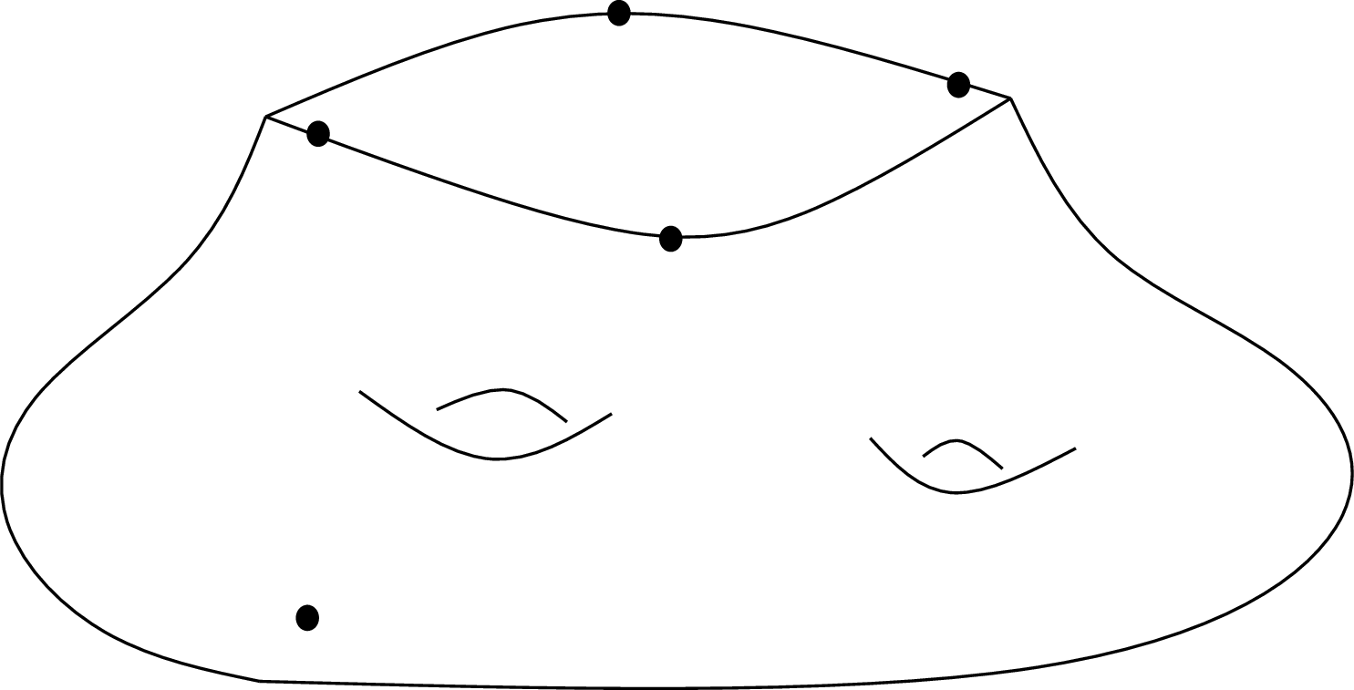
A decorated surface \({\Bbb S}\) is a connected oriented topological surface with boundary circles, and a finite number of marked points on the boundary, considered modulo isotopy. We sometimes refer to the boundary circles without marked points as punctures, see Figure 1, and to the marked points as cusps.
Denote by \({\rm D}_n^*\) a once punctured disc with \(n\) marked boundary points, see the left picture on Figure 2.
A hyperbolic crown is the decorated surface \({\rm D}_n^*\) with a hyperbolic structure, which is bordered on the one side by the crown end - a collection of bi-infinite geodesics such that each adjacent pair forms a cusp - and on the other side by the unique geodesic, called the neck geodesic, plus a horocycle near each cusp, see the middle picture on Figure 2. The universal cover of the hyperbolic crown is shown on the right of Figure 2. A fundamental domain for the deck transformation action of the fundamental group \({\mathbb{Z}}\) is a geodesic \((n+3)-\)gon in the hyperbolic plane, bounded by the universal cover \(\widetilde{\gamma}\) of the neck geodesic \(\gamma\).

Definition 1. An ideal hyperbolic structure* on a decorated surface \({\Bbb S}\) is a hyperbolic metric of curvature \(-1\) on \({\Bbb S}\) with the following boundary structure, illustrated on Figure 3:*
Each boundary circle without marked points is a geodesic.
The hyperbolic metric near each boundary component with marked points is a crown end.
A choice of a horocycle \(h_p\) near each cusp \(p\).

Let us now introduce the moduli spaces which we study in the paper.
Definition 2.
The Teichmüller space \(\mathcal{T}_{\Bbb S}\) of a decorated surface \({\Bbb S}\) parametrises ideal hyperbolic structures on \({\Bbb S}\), up to orientation and boundary preserving homeomorphisms of \({\Bbb S}\) isotopic to the identity.
The pure mapping class group \({\rm Mod}({\Bbb S})\) is the quotient of the group of orientation \(\&\) boundary preserving homeomorphisms of \({\Bbb S}\) modulo the ones isotopic to the identity. The moduli space of \(\mathcal{M}_{\Bbb S}\) is the quotient \[\mathcal{M}_{\Bbb S}:= \mathcal{T}_{\Bbb S}/{\rm Mod}({\Bbb S}).\]
Here are a few examples and comments.
When \({\Bbb S}\) is a disc with \(n\) marked points, an ideal hyperbolic structure on \({\Bbb S}\) describes a collection of \(n\) horocycles in the hyperbolic disc. Each horocycle defines a point on the boundary circle, and we connect each pair of adjacent points by a bi-infinite geodesic. The Teichmüller space \({\cal T}_{\Bbb S}\) parametrises ideal \(n-\)gons with horocycles at the vertices, see Figure 4. The group \({\rm Mod}({\Bbb S})\) is trivial. So \(\mathcal{M}_{\Bbb S}= \mathcal{T}_{\Bbb S}\).
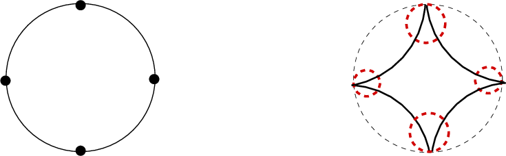
When \({\Bbb S}={\rm D}^*_n\) is a punctured disc with \(n\) marked points, the Teichmüller space \({\cal T}_{{\rm D}_n^*}\) parametrises hyperbolic crowns with \(n\) cusps, see Figure 2. The group \({\rm Mod}({\Bbb S})\) is trivial. So \(\mathcal{M}_{\Bbb S}= \mathcal{T}_{\Bbb S}\).
When \({\Bbb S}\) does not have any crown end, the Teichmüller space \(\mathcal{T}_{\Bbb S}\) is the usual Teichmüller space.
The classical Teichmuller space \({\cal T}^{\rm cl}_{\Bbb S}\) parametrises hyperbolic structures on \({\Bbb S}\) with geodesic boundary and crown ends, see [1]. There is a canonical \({\rm Mod}({\Bbb S})-\)equivariant isomorphism \[{\cal T}_{\Bbb S}\stackrel{\sim}{\longrightarrow} {\cal T}^{\rm cl}_{\Bbb S}\times {\mathbb{R}}^{\{\rm cusps p on {\Bbb S}\}}.\] The projection onto \({\cal T}^{\rm cl}_{\Bbb S}\) forgets the horoarcs. The map onto the second factor is given by the areas of domains enclosed between the cusps \(p\) and the horoarcs \(h_p\). It plays the crucial role in the story.
Consider the decorated Teichmuller space \({\cal T}^{\rm d}_{\Bbb S}\) parametrising ideal hyperbolic structures on \({\Bbb S}\) where geodesic boundary circles are reduced to punctures, that is have zero length, and equipped with horocycles. For a punctured surface without boundary we get Penner’s decorated Teichmuler space [2]. The Teichmuller spaces \({\cal T}_{\Bbb S}\) and \({\cal T}^{\rm d}_{\Bbb S}\) are dual to each other. In particular \({\rm dim}{\cal T}_{\Bbb S}= {\rm dim}{\cal T}^{\rm d}_{\Bbb S}\). This duality is a manifestation of the cluster duality [3], see Section 2.
A decorated surface \({\Bbb S}\) carries a collection of isotopy classes of simple loops, isotopic to the boundary circles, with or without marked points. We call them boundary loops of \({\Bbb S}\). Given an ideal hyperbolic structure on \({\Bbb S}\), each boundary loop is represented by the neck geodesic. If a boundary component is not a crown, the neck geodesic is the boundary geodesic loop. We denote by \(m\) the number of boundary components of \({\Bbb S}\), by \(l_1, \ldots, l_m\) the lengths of the neck geodesics, and by \(r\) the number of boundary components with marked points.
For each boundary geodesic connecting two adjacent cusps at the ends of a boundary interval \({\rm F}\), we define its length \(\kappa_{{\rm F}}\in {\mathbb{R}}\) as the distance between the two horocycles at the cusps, taken with the minus sign if the horocycles overlap. We call it the signed distance. Let us define the \({\rm K}-\)coordinate1
\[\label{KF} {\rm K}_{{\rm F}}:= e^{-\kappa_{{\rm F}}}.\tag{1}\]
Take an ideal hyperbolic structure on a decorated surface \({\Bbb S}\) with ideal crowns \({\rm C}_1,\ldots, {\rm C}_r\). Given an ideal crown \({\rm C}_i\) with \(n_i\) cusps, there are \({\rm K}-\)coordinates \({\rm K}_{{\rm C}_i, j}\), \(1 \leq j \leq n_i\) at the boundary intervals of the crown. They are positive numbers. We denote by \({{\rm K}}\) the collection of these numbers: \[\label{KC} {{\rm K}}:= \{{{\rm K}}_{{{\rm C}_i}}\}, \qquad {{\rm K}}_{{{\rm C}_i}}:=({{\rm K}}_{{{\rm C}}_{i, 1}},..., {{\rm K}}_{{{\rm C}}_i, n_i})\in {\Bbb R}^{n_i}_{>0}.\tag{2}\]
We denote the geodesic lengths of the boundary geodesic circles by \[\label{spL} {\rm L}=(l_{r+1},...,l_{m})\in {\mathbb{R}}_{\geq 0}^{m-r}.\tag{3}\]
Definition 3. The Teichmüller space \({\cal T}_{\Bbb S}({{\rm K}}, {\rm L})\) is the subspace of the Teichmüller space \({\cal T}_{\Bbb S}\) with the given set \({{\rm K}}\) of \({\rm K}-\)coordinates (2 ), and the given set \({\rm L}\) of lengths of the boundary geodesic circles (3 ).
The moduli space \(\mathcal{M}_{\Bbb S}({\rm K}, {\rm L})\) is the quotient: \[\label{MS} \begin{align} &\mathcal{M}_{\Bbb S}({{\rm K}}, {\rm L}):= \mathcal{T}_{\Bbb S}({{\rm K}}, {\rm L})/{\rm Mod}({\Bbb S}).\\ \end{align}\qquad{(1)}\] We denote by \(\mathcal{T}_{\Bbb S}({{\rm K}})\) and \(\mathcal{M}_{\Bbb S}({{\rm K}})\) the Teichmüller and moduli space when \({\rm L}\) is not fixed.
If \({\Bbb S}\) is a genus \(g\) surface without marked points and with \(m\) boundary circles of zero lengths, we get the moduli space \({\cal M}_{g,m}\).
1.1.2 The exponential volumes.↩︎
Recall that an ideal hyperbolic structure on \({\Bbb S}\) carries a horoarc \(h_p\) at each cusp \(p\). We denote by \(W_p\) the area enclosed by the horoarc \(h_p\). We call it the local potential at the cusp \(p\), or just the potential at the cusp \(p\). The potential \(W_{\Bbb S}\) is a function on the Teichmüller space \({\cal T}_{\Bbb S}\) given by the sum of the potentials at all cusps on \({\Bbb S}\): \[W_{\Bbb S}:= \sum_{p}W_p.\] Both the local potentials \(W_p\) and the potential \(W_{\Bbb S}\) are \({\rm Mod}({\Bbb S})-\)invariant. Therefore they are functions on the moduli space (?? ).
Given an orientation of the Teichmüller space \(\mathcal{T}_{\Bbb S}\), there is canonical volume form \(\Omega_{\Bbb S}\) on \(\mathcal{T}_{\Bbb S}\), with positive integrals over discs. It has a simple expression (33 ) in the cluster Poisson coordinates. It is \({\rm Mod}({\Bbb S})-\)invariant, and induces a volume form \(\Omega_{\Bbb S}({{{\rm K}}, {\rm L}})\) on the moduli space \(\mathcal{M}_{\Bbb S}({{\rm K}}, {\rm L})\) as in equation (48 ). When \({\Bbb S}\) has no marked points, it is propotional to the Weil–Petersson volume form. The exponential volume form is a positive measure on the oriented Teichmüller space \(\mathcal{T}_{\Bbb S}\) given by \[\label{6} e^{-W_{\Bbb S}}\Omega_{\Bbb S}({{{\rm K}}, {\rm L}}).\tag{4}\]
Definition 4. The exponential volume of the moduli space \(\mathcal{M}_{\Bbb S}({{\rm K}}, {\rm L})\) is given by \[\label{EXV} {\rm Vol}_{{\mathcal{E}}}\mathcal{M}_{\Bbb S}({{\rm K}}, {\rm L}):=\int_{\mathcal{M}_{\Bbb S}({{\rm K}}, {\rm L})} e^{-W_{\Bbb S}}\Omega_{\Bbb S}({{{\rm K}}, {\rm L}}).\qquad{(2)}\]
1.1.3 Mirzakhani’s volume formula.↩︎
When \({\Bbb S}=S\) has no marked points, the potential \({W}_S\) is zero, and the set \({\rm K}\) is empty. Then we write \(\Omega_S({\rm L})\) for the cluster form (
4 ). It is proportinal to the Weil–Petersson volume form: \[\label{WPCL} \Omega_S({\rm L}) = d_S\Omega^{\rm WP}_S({\rm L}), \;\;\;\;d_S \in {\mathbb{Q}}^*_+,\tag{5}\] for some positive rational constant \(d_S\).2 So we get the Weil-Peterssen volume of the moduli space \(\mathcal{M}_S({\rm L})\) of genus \(g\) hyperbolic surfaces with fixed boundary geodesic lengths \({\rm L}= (l_1, ..., l_m)\): \[{\rm Vol}_{\rm WP}(\mathcal{M}_S)({\rm L}):= \int_{\mathcal{M}_S({\rm L})} \Omega^{\rm WP}_S({\rm L}).\] By Mirzakhani’s theorem [5] it is an even polynomial in \(l_i\) of degree \(6g-6+2m\): \[\label{V1} {\rm Vol}_{\rm WP}(\mathcal{M}_S({\rm L})) = \sum_{d_1+ \ldots + d_m \leq d} {\cal V}_{g, d_1, ..., d_m}l_1^{2d_1} \ldots l_m^{2d_m}, \;\;\;\;d:= 3g-3+m = \frac{1}{2}{\rm dim}_{\mathbb{R}}{\cal M}_S({\rm L}).\tag{6}\] Here \(d_i\geq 0\) are integers. Setting \(|d|:= d_1+\ldots + d_m\) and \(q:=d-|d|\), we have \[\label{NV} {\cal V}_{g, d_1, ..., d_m} \in \pi^{2q}{\Bbb Q}.\tag{7}\] By [5], we have \[\label{WCM} {\cal V}_{g, d_1, ..., d_m} = \frac{1}{2^{|d|}|d|! q!}\cdot \int_{\overline{\cal M}_{g,m}}\psi_1^{d_1}\cdots \psi_m^{d_m}\omega^{q}.\tag{8}\] Here \(\psi_i\) is the first Chern class of the line bundle on \(\overline{\cal M}_{g,m}\) given by the tangent space at the \(i-\)th puncture on the curve, and \(\omega\) is the Weil–Petersson symplectic form on \(\overline{\cal M}_{g,m}\).
So the leading coefficients are rational numbers - the intersection numbers of the \(\psi-\)classes on \(\overline{\cal M}_{g,m}\).
1.1.4 The first main result.↩︎
If \({\Bbb S}\) has marked points, the volume is always infinite. In contrast with this we prove in Section 3.3:
Theorem 1. For any decorated surface \({\Bbb S}\), the exponential volume \({\rm Vol}_{{\mathcal{E}}}\mathcal{M}_{\Bbb S}({{\rm K}}, {\rm L})\) is finite.
Theorem 1 supports the main idea of this paper:
The moduli spaces \({\cal M}_{{\Bbb S}}({{\rm K}}, {\rm L})\) with the exponential volume forms are the true analogs of the moduli spaces \({\cal M}_{g,n}\) and \({\cal M}_S({\rm L})\) with the Weil–Petersson volume forms.
For instance the Weil–Petersson volume forms are essential in the string theory [6] as the background measures for the correlation functions/volume forms on \({\cal M}_{g,m}\). The exponential volume form should play a similar role in the open string theory.
1.2 The Laplace transform of exponential volumes and \({\cal B}-\)functions↩︎
1.2.1 The Laplace transform of exponential volumes.↩︎
Take a collection of complex numbers \[s=(s_1, \ldots, s_m)\in {\mathbb{C}}^m.\] Recall the set of parameters \({\rm K}\) from (2 ). Denote by \[{\rm L}= (l_1, \ldots, l_m)\in {\mathbb{R}}_{+}^m\] the lengths of all neck geodesics, including the boundary geodesics. We denote by \(\Omega_{\Bbb S}({\rm K})\) the volume form on the space \(\mathcal{M}_{\Bbb S}({{\rm K}})\), where \({\rm L}\) is not fixed. Consider the following integral: \[\label{EIIa} \begin{align} {\mathcal{L}}_{\Bbb S}({{\rm K}}; s_1, ..., s_m, \hbar) :=& \int_{{\cal M}_{\Bbb S}}e^{-W/\hbar}\;e^{-(l_1 s_1 + \ldots +l_m s_m)/2}\Omega_{\Bbb S}({{\rm K}}). \\ \end{align}\tag{9}\]
::: {#MTHOEE* .lemma} Lemma 1. For any decorated surface \({\Bbb S}\), the integral (9 ) is convergent for \({\rm Re}(s_i)\geq 0\), and has an analytic continuation to a meromorphic function in \(s\). :::
Proof. This is proved in Theorem 19. Alternatively, the convergence of the integral for \({\rm Re}(s_i)\geq 0\) follows from the finiteness of the exponential volume, see Theorem 1. Then the analytic continuation and its properties follow from the standard properties of the distribution \(x_+^\lambda\) on \({\mathbb{R}}\), applied to \({\rm L}_i^{s_i}\) [7]. ◻
The function (9 ) generalizes the Laplace transform of the classical volumes \({\rm Vol}(\mathcal{M}_S({\rm L}))\) in (6 ).
Let us note that Mirzakhani’s recursions for these volumes are equivalent to the Eynard–Orantin Topological Recursion for the Laplace transform of the volumes, for a certain spectral curve [8]. The complex variables \(s_1, \ldots , s_m\) become the points on the spectral curve.
1.2.2 \({\cal B}-\)function of a decorated surface \({\Bbb S}\).↩︎
It is a similar integral: \[\label{EIa} \begin{align} {\mathcal{B}}_{\Bbb S}({{\rm K}}; s_1, ..., s_m; \hbar) := & \int_{{\cal M}^{\circ \circ}_{\Bbb S}}e^{-W/\hbar}\;e^{-(l_1 s_1 + \ldots +l_m s_m)/2}\Omega_{\Bbb S}({{\rm K}}).\\ \end{align}\tag{10}\] The integration is over the \(2^{r}:1\) ramified cover \({\cal M}^{\circ \circ}_{\Bbb S}\) of \({\cal M}_{\Bbb S}\), obtained by specifying an eigenvalue of the monodromy around each crown neck geodesic. Their logarithms \(l_1, ..., l_r\) can be any real numbers. So \[(l_1, ..., l_r, l_{r+1}, ..., l_{m}) \in {\mathbb{R}}^r\times {\mathbb{R}}_+^{m-r}.\]
The \({\cal B}-\)function is the sum of \({\cal L}-\)functions, over all \(2^r\) ways to put the signs: \[{\mathcal{B}}_{\Bbb S}({{\rm K}}; s_1, ..., s_m;\hbar) = \sum {\mathcal{L}}_{\Bbb S}({{\rm K}}; \pm s_1, ..., \pm s_r, s_{r+1}, ..., s_m; \hbar).\] Below we often specialize \(\hbar=1\), skipping \(\hbar\) from the notation.
Recall the modified Bessel function of the second kind, which we refer to below as the Bessel function3: \[\label{f22} \begin{align} J_s(z):=&\int_{0}^\infty {\rm exp}\Bigl({-\sqrt{z}(\lambda+\lambda^{-1}} )\Bigr)\lambda^{s} d\log {\lambda}\\ =&z^{-s/2}\cdot \int_{0}^\infty {\rm exp}\Bigl({-t-\frac{z}{t}} \Bigr)t^{s} d\log {t}.\\ \end{align}\tag{11}\] Note that it is an even function in \(s\): \(J_s(z)=J_{-s}(z)\).
There are important special cases of the function \({\cal B}_{\Bbb S}\), when it reduces to the Bessel function.
When \({\Bbb S}= {\rm D}_1^*\) is a punctured disc with one cusp, we get the Bessel function \[\label{213} \mathcal{B}_{{\rm D}^*_1}({{\rm K}}; s) = 2 J_{s}({\rm K}).\tag{12}\] Indeed, the moduli spaces of enhanced ideal hyperbolic structures on \({\rm D}_1^*\) is parametrised by pairs of real numbers \((\kappa, l)\), where \(\kappa\) is the length of the crown geodesic between its intersections with the horocycle, and \(l\in {\mathbb{R}}\) is the signed length of the neck geodesic. We use the exponential coordinates \[{\rm K}= e^{-\kappa}, \;{\rm L}=e^{l}.\] The potential function at the cusp is calculated in Proposition 5 below: \[\label{EXVtI*} \begin{align} W_{ {{\rm D}_1^*} }({\rm K}, l) = \;&{\rm K}^{1/2} (e^{l/2} +e^{-l/2} ).\\ \end{align}\tag{13}\] The volume form \(\Omega_{ {{\rm D}_1^*}}= d\log {\rm L}^{1/2}\). Therefore by the very definition of the \({\cal B}-\)function: \[\label{FBFa} \mathcal{B}_{{\rm D}^*_1}({{\rm K}}; s) := 2 \int_{-\infty}^\infty {\rm exp}(-{\rm K}^{1/2} (e^{l/2} +e^{-l/2} ))e^{-ls/2}d(l/2) =2J_{s}({\rm K}).\tag{14}\]
When \({\Bbb S}= {\rm D}_n^*\) is a punctured disc with \(m\) cusps, the \({\cal B}-\)function is a product of Bessel functions: \[\label{GC} \mathcal{B}_{{\rm D}^*_n}({{\rm K}_1, ..., {\rm K}_n}; s) = 2 J_{s}({\rm K}_1)\cdots J_{s}({\rm K}_n).\tag{15}\] We prove this in Example 1 of Section 3.
1.2.3 The function \({\cal B}_{\Bbb S}\) via \({\rm A}-\)model.↩︎
a) According to Givental [9], see also [10], the Bessel function \(J_s({\rm K})\) solves the quantum differential equation for the \({\Bbb C}^\times-\) equivariant quantum cohomology \({\rm QH}^*_{{\Bbb C}^\times}({\Bbb C}{\rm P}^1)\), where \({\mathbb{C}}^\times\) acts by preserving points \(\{0, \infty\} \subset {\mathbb{C}}{\rm P}^1\). Here \({\rm K}\) is the Kähler parameter, and \(s\) the \({\mathbb{C}}^\times-\)equivariant parameter.4
b) Givental’s theorem, combined with (15 ), tells that the function \(\mathcal{B}_{{\rm D}^*_n}({{\rm K}_1, ..., {\rm K}_n}, s)\) solves the quantum differential equation for the \({\Bbb C}^\times-\)equivariant quantum cohomology \[{\rm QH}^*_{{\Bbb C}^\times}({\Bbb C}{\rm P}^1\times \cdots \times {\Bbb C}{\rm P}^1)\] of the product of \(n\) copies of \({\Bbb C}{\rm P}^1\). Here \({\rm K}_1, ..., {\rm K}_n\) are Kähler parameters, and \(s\) the equivariant parameter. In particular, the function \({\cal B}_{\Bbb S}\) is related to an \({\rm A}-\)model interpretation.
c) If \({\Bbb S}=S\) is a genus \(g\) surface with \(m\) punctures, Mirzakhani’s formula (8 ) calculates the volume in terms of the \({\rm A}-\)model on \({\cal M}_{g,m}\).
It would be very interesting to find an \({\rm A}-\)model interpretation of the function \({\cal B}_{\Bbb S}\) for the general \({\Bbb S}\). The key
problem is that in general the group \({\rm Mod}({\Bbb S})\) is infinite, while in the examples a), b) it is trivial.
1.3 Neck recursion formula↩︎
Our next goal is a recursion formula which allows us to calculate the exponential volume integrals.
Let us cut \({\Bbb S}\) along a neck geodesic \(\ell\): \[{\Bbb S}= {\rm D}_{\ell} \cup {\Bbb S}_{\ell}; \quad {\Bbb S}_{\ell}:= {\Bbb S}-{\rm D}_{\ell}.\] Here \({\rm D}_{\ell}\) is a decorated surface given by a punctured disc with \(k\) cusps. Denote by \(l\) the length of \(\ell\). Since the neck geodesic \(\ell\) is a boundary component of both surfaces \({\rm D}_{\ell}\) and \({\Bbb S}_{\ell}\), the exponential volumes \({\rm Vol}_{\cal E}({\cal M}_{{{\rm D}}_{\ell}})\) and \({\rm Vol}_{\cal E}({\cal M}_{{\Bbb S}_{\ell}})\) depend on \(l\).
Theorem 2. Let \({\rm C}_{{\Bbb S}, \ell}:=2^{-\mu_\ell} c_{{\Bbb S}, \ell}\) where \(\mu_\ell\) is the number of one-holed tori cut off by \(\ell\) and \(c_{{\Bbb S}, \ell}\) is a positive constant depending only on \({\Bbb S}\) and \(\ell\) defined in Proposition 17. One has the following neck recursion formula: \[\label{NRF1} \begin{align} & {\rm Vol}_{\cal E}({\cal M}_{\Bbb S})({\rm K},{\rm L}) = {\rm C}_{{\Bbb S}, \ell} \int^\infty_{0} {\rm Vol}_{\cal E}({\cal M}_{{{\rm D}}_{\ell}})({\rm K}_{\rm D_\ell}) \cdot {\rm Vol}_{\cal E}({\cal M}_{{\Bbb S}_{\ell}})({\rm K}',{\rm L}') \;ldl,\\ \end{align}\qquad{(3)}\] \[\label{NRF2*} \begin{align} & {\cal L}_{\Bbb S}({{\rm K}}; s_1, ..., s_m) = {\rm C}_{{\Bbb S}, \ell} \int^\infty_{0} {\rm Vol}_{\cal E}({\cal M}_{{{\rm D}}_{\ell}})({\rm K}_{\rm D_\ell}) \cdot {\cal L}_{{\Bbb S}_{\ell}}({\rm K}'; s_1, ..., s_{m}) \;l dl.\\ \end{align}\qquad{(4)}\]
Theorem 2 is proved in Section 2.2.5.
Theorem 2, combined with Mirzakhani’s formula (6 ), has the following two applications.
1. It allows us to express the function \({\cal B}_{\Bbb S}({{\rm K}}; s)\) as a linear combination with coefficients in the ring \[\label{RR} {\mathbb{Q}}[\pi^2, s_{r+1}^{-1}, ... , s_m^{-1}]\tag{16}\] of the product of odd derivatives of Bessel functions, generalizing formula (15 ). Precisely, consider the following differential operator in \(s_1, ..., s_r\), where \({\cal V}_{g, d_1, ..., d_m}\in {\mathbb{Q}}[\pi^2]\) were defined in (6 ): \[\label{DS} {\cal D}_{\Bbb S}:= \sum_{d_1+ ... + d_m\leq 3g-3+m} 2^{m} \;{\cal V}_{g, d_1, ..., d_m} \Bigl(-2\frac{d}{ds_1}\Bigr)^{2d_1+1}\cdots \Bigl(-2\frac{d}{ds_r}\Bigr)^{2 d_r+1}\cdot \prod_{j=r+1}^m\frac{(2d_j)!}{s_j^{2d_j+1}}.\tag{17}\] Denote by \({\boldsymbol{K}}_j\) the product of the \({\rm K}-\)coordinates at the \(j-\)th boundary component of \({\Bbb S}\).
Theorem 3. The function \({\cal B}_{\Bbb S}\) is obtained by applying operator (17 ) to the product of Bessel functions: \[\label{MFOEaaa} \begin{align} &{\cal B}_{{\Bbb S}}({{\rm K}}, s_1, ..., s_r) = {\rm C}_{{\Bbb S}} \cdot {\cal D}_{{\Bbb S}} \;\prod_{j=1}^r J_{s_j}({\boldsymbol{K}}_j), \;\;\;\; {\rm C}_{\Bbb S}:= \prod_{i=1}^r {\rm C}_{{\Bbb S},\ell_i}.\\ \end{align}\qquad{(5)}\]
Theorem 3 is proved in Section 3.
2. Setting \(s_1=...=s_r=0\), Theorem 3 allows us to express the exponential volumes as linear combinations with coefficients in the ring (16 ) of odd derivatives of Bessel like integrals at \(s=0\), see Theorem 21 combined with formula (72 ). Each of the terms is manifestly a period of exponential mixed motive, discussed in Section 1.6.
Our main result is a different way to express the exponential volume integrals via integrals over the products of the moduli spaces with simpler topology, which we call unfolding formulas.
1.4 Unfolding exponential volumes↩︎
The unfolding starts from a choice of a cusp \(p\) on \({\Bbb S}\), and consists of two steps.
1.4.1 Reduction to the case when \(p\) is single cusp on a crown.↩︎
There is a unique up to an isotopy arc \(\pi_p\) from the cusp \(p\) to itself, which is homotopic to the boundary component containing \(p\). Cutting \({\Bbb S}\) along it, we get a disjoint union of a polygon \({\rm P}_p\) and a decorated surface \({\Bbb S}_p = {\Bbb S}-{\rm P}_p\): \[{\Bbb S}- \pi_p = {\rm P}_p \cup {\Bbb S}_p.\] The surface \({\Bbb S}_p\) inherits a single cusp \(p\) on the crown \({\rm C}_p\) bounded by \(\pi_p\). If the crown of \({\Bbb S}\) containing the cusp \(p\) has \(n\) sides with the \({\rm K}-\)coordinates \({\rm K}_1, ..., {\rm K}_n\) assigned to them, the polygon \({\rm P}_p\) is an \((n+1)-\)gon with the \({\rm K}-\)coordinates \({\rm K}_1, ..., {\rm K}_n, {\rm K}\). The decorated surface \({\Bbb S}_p\) has a single boundary interval on the crown \({\rm C}_p\) containing \(p\), with the \({\rm K}-\)coordinate \({\rm K}\) assigned to it.
Proposition 4. One has \[\label{recurP} \begin{align} &{\rm Vol}_{\cal E}({\cal M}_{\Bbb S})= \int_{\mathbb{R}_+} {\rm{Vol}}_{\mathcal{E}}({\cal M}_{ {{\rm P}_p}})({\rm K}_1, \ldots , {\rm K}_n, {\rm K}) \cdot{ \rm{Vol}}_{\mathcal{E}}({\cal M}_{{\Bbb S}_p})({\rm K}, \ldots)\; d\log {\rm K}. \\ \end{align}\qquad{(6)}\]
Proposition 4 follows immediately from the cutting and gluing formulas for the exponential volume forms in Sections 2.2 and 5.1.
From now on, we assume that \(p\) is a single cusp on a certain crown of \({\Bbb S}\), denoted by \({\rm C}_p\).
1.4.2 Trouser legs and ideal triangles at a cusp \(p\).↩︎
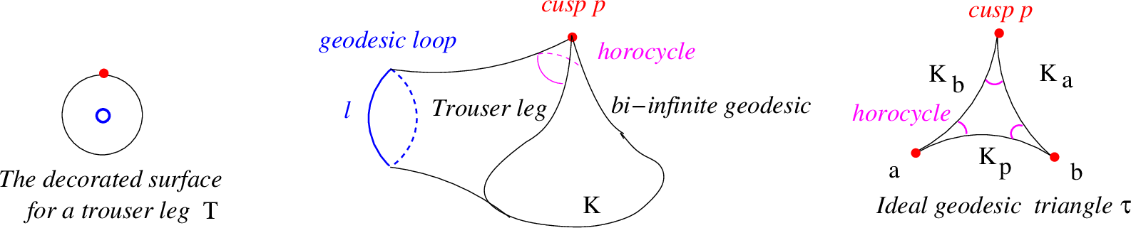
We call a decorated surface \({\Bbb S}\) is elementary, if the moduli space \({\cal M}_{\Bbb S}({\rm K}, {\rm L})\) is a point. There are three of them: a punctured disc \({\rm D}_1^*\) with a special point, a triangle, and a pair of pants. We refer to the first two, embedded as decorated surfaces into a decorated surface \({\Bbb S}\), as trouser legs and ideal triangles, respectively. So the elementary decorated surfaces containing the cusp \(p\), see Figure 5, are:
Trouser legs \({\rm T}\subset {\Bbb S}\), containing the cusp \(p\).
Ideal triangles \(\tau\subset {\Bbb S}\) and containing the cusp \(p\).
1.4.3 Unfolding for a crown with a single cusp \(p\).↩︎
The moduli spaces \({\cal M}_\tau({\rm K}_a, {\rm K}_b, {\rm K}_p)\) and \({\cal M}_{{\rm T}}({\rm K}, l)\) of ideal hyperbolic structures on a triangle \(\tau({\rm K}_a, {\rm K}_b, {\rm K}_p)\) and a trouser leg \({\rm T}({\rm K},l)\) with \({\rm K}-\)coordinates \(({\rm K}_a, {\rm K}_b, {\rm K}_p)\) and \(({\rm K}, l)\), see Figure 5, are points. Yet their exponential volumes are non-trivial functions of \({\rm K}-\)coordinates denoted by \({\cal E}_\tau\) and \({\cal E}_{{\rm T}}\). Precisely, let \(W_\tau\) and \(W_{\rm T}\) be the potentials of a triangle \(\tau\) and a trouser leg \({\rm T}\). Then by Corollaries 1 and 2 \[\label{eqelevol} \begin{align} &{\cal E}_{\tau}({\rm K}_a, {\rm K}_b, {\rm K}_p):= e^{-W_{\tau}}; \;\;\;\;\;\;\;\;\;\; {\cal E}_{\rm T}({\rm K}, l):= e^{-W_{\rm T}}. \\ \end{align}\tag{18}\]
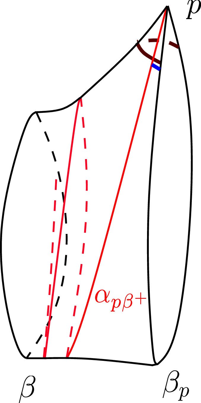
Next, let \(W_{\tau, p}\) be the partial potential of a triangle \(\tau\) at the cusp \(p\). For a trouser leg \({\rm T}\) with a cusp \(p\), let \(Q_{{\rm T}}({\rm K}, l)\) be the area of the triangle cut by the horocycle \(h_p\) at \(p\), the boundary geodesic \(\beta_p\), and the geodesic \(\ell_{p\beta^+}\) from \(p\) circling around the geodesic boundary loop \(\beta = \ell_{\rm T}\) of \({\rm T}\), see Figure 6. We have:
Proposition 5. For an ideal triangle \(\tau({\rm K}_a, {\rm K}_b, {\rm K}_p)\) and a trouser leg \({\rm T}({\rm K},l)\) with a cusp \(p\) one has \[\label{gapfunctI} \begin{align} {W}_{\tau, p}({\rm K}_a, {\rm K}_b, {\rm K}_p)\;&= \; \Bigl(\frac{{\rm K}_a{\rm K}_b}{{\rm K}_p}\Bigr)^{1/2}, \\ W_{\tau}({\rm K}_a, {\rm K}_b, {\rm K}_p) \;&:= \;{W}_{\tau, p} + {W}_{\tau, a} +{W}_{\tau, b}, \\ Q_{{\rm T}}({\rm K}, l) \;&={\rm K}^{1/2}e^{-l/2},\\ W_{ {{\rm T}} }({\rm K}, l) \;&= \;{\rm K}^{1/2} (e^{l/2} +e^{-l/2} ).\\ \end{align}\qquad{(7)}\]
For the formula in the first line see (39 ); it goes back to [11], see also [12]. The formula in the second line is just a definition. The last two formulas are proved in Lemmas 11 and 12.
Given a cusp \(p\), we introduce recursion kernel functions \({\cal R}_{\zeta, p}\) for the ideal triangles \(\zeta=\tau({\rm K}_a, {\rm K}_b, {\rm K}_p)\) and trouser legs \(\zeta ={\rm T}({{\rm K}},l)\) containing \(p\): \[\label{gapfunctII} \begin{align} &{\cal R}_{\tau, p}({\rm K}_a, {\rm K}_b, {\rm K}_p):= {W}_{\tau, p}\;\;\stackrel{(\ref{gapfunctI})}{=} \; \;\Bigl(\frac{{\rm K}_p}{{\rm K}_a{\rm K}_b}\Bigr)^{-1/2}, \\\ &{\cal R}_{{\rm T}, p}({\rm K}, l):= \left\{ \begin{array}{lll} { {\rm K}}^{1/2} (e^{l/2} +e^{-l/2} ), \;\;\; \; \;\;\; \;\; if the geodesic loop \ell_{\rm T}\subset \partial {\Bbb S}.\\ 2^{1-\mu_{{\rm T}}}{{\rm K}}^{1/2}e^{-l/2}, \; \; \;\;\;\; \qquad if the geodesic loop \ell_{\rm T}\not \subset \partial {\Bbb S}.\\ \end{array}\right.\\ \end{align}\tag{19}\] Here \(\mu_{{\rm T}}\) is the number of one-holed tori cut out by a trouser leg \(\rm T\).
A function \(f\) on the moduli space \({\cal M}_{\Bbb S}({{\rm K}}, {\rm L})\) is just a \({\rm Mod}({\Bbb S})-\)invariant function on the Teichmüller space \({\cal T}_{\Bbb S}({{\rm K}}, {\rm L})\). So it provides a function on Teichmuller spaces \({\cal T}_{{\Bbb S}- \tau}\) and \({\cal T}_{{\Bbb S}- {\rm T}}\), also denoted by \(f\).
Given an elementary surface \(\zeta\subset {\Bbb S}\) containing the cusp \(p\), consider the fibered product of Teichmuller spaces over the base \({\cal C}_{\zeta, {\Bbb S}}\), provided by the common boundary components of \(\zeta\) and \({\Bbb S}-\zeta\): \[\label{FP} {\cal T}_{\zeta}\times_{{\cal C}_{\zeta, {\Bbb S}}} {\cal T}_{{\Bbb S}-\zeta }.\tag{20}\] The base \({\cal C}_{\zeta, {\Bbb S}}\) is parametrised as follows, where \(\ell_{\rm T}\) is the geodesic boundary loop of a trouser leg \({\rm T}\subset {\Bbb S}\):
If \(\zeta = \tau\): by the \({\rm K}-\)coordinates on internal edges of \(\zeta\).
These are \({\rm K}_a\) if there is one internal edge, and \(({\rm K}_a, {\rm K}_b)\) if there are two.
If \(\zeta ={\rm T}\): by the \({\rm K}-\)coordinate \({\rm K}_a\) if \(\ell_{\rm T}\subset \partial {\Bbb S}\), and by the \(({\rm K}_a, l, \theta)\) if \(\ell_{\rm T}\not \subset \partial {\Bbb S}\).
In the latter case, \((\theta, l)\) are the Fenchel–Nielsen coordinates related to the loop \(\ell_{\rm T}\).
Let \(c_{{\Bbb S},\ell_{\rm T}}\) be some positive rational constant depending only on \({\Bbb S}\) and \(\ell_{\rm T}\) as in Proposition 17. There is the following canonical volume form on the base \({\cal C}_{\zeta, {\Bbb S}}\): \[\label{formvol} \begin{align} & {\rm vol}_{{\cal C}_{\zeta, {\Bbb S}}} = \left\{ \begin{array}{lll} d\log {\rm K}_a \;\;\; \; \;\; \;\;\; \;\; \; \; \;\;\; \; \;\;\;\;\;if \zeta = {\rm T} and \ell_{\rm T}\subset \partial {\Bbb S},\\ c_{{\Bbb S},\ell_{\rm T}} \cdot dl \wedge d\theta\wedge d\log {\rm K}_a \; \; if \zeta = {\rm T} and \ell_{\rm T}\not \subset \partial {\Bbb S}, \\ d\log {\rm K}_a \; \;\;\;\; \;\; \; \;\; \;\; \; \;\; \; \;\; \;\;\;\;if \zeta = \tau with one internal side with coordinate {\rm K}_a,\\ d\log {\rm K}_a \wedge d\log {\rm K}_b \;\; \;\; \;\;\;\; \;if \zeta = \tau is with two internal sides with coordinates {\rm K}_a, {\rm K}_b.\\ \end{array}\right.\\\end{align}\tag{21}\]
We use the shorthand for the exponential volume form on the space \({\cal M}_{\Bbb S}({{\rm K}}, {\rm L})\) from Definition 3: \[\label{OKL} {\Bbb E}_{{\Bbb S}}:= {\Bbb E}_{{\Bbb S}}({\rm K}, {\rm L}) := e^{-W_{\Bbb S}} \;\Omega_{\Bbb S}({{\rm K}}, {\rm L}).\tag{22}\]
The pure mapping class group \({\rm Mod}({\Bbb S})\) fixes the cusps. So it acts on isotopy classes of elementary decorated surfaces \(\zeta\) containing the cusp \(p\). There are finitely many \({\rm Mod}({\Bbb S})-\)orbits. Indeed, an orbit is determined by the topology of the surface \({\Bbb S}-\zeta\), and there are only finitely many topological types of surfaces. Let us consider the following finite set.
- The set \([{\cal H}_{{\zeta}, p}]\) of \({\rm Mod}({\Bbb S})-\)orbits on the set of isotopy classes of elementary decorated surfaces \({\zeta}\subset {\Bbb S}\) containing the cusp \(p\). Here if \(\zeta\) is an ideal triangle, we assume that its side opposite to \(p\) is a boundary interval of \({\Bbb S}\). We call such triangles the \(p-\)narrowest triangles.
Denote by \({\rm Stab}_\zeta\) the stabiliser of the elementary decorated surface \(\zeta\subset {\Bbb S}\) in \({\rm Mod}({\Bbb S})\). Let us set \[\label{MZETA} {\cal M}_{{\Bbb S}, \zeta}({\rm K}, {\rm L}):= {\cal T}_{{\Bbb S}}({\rm K}, {\rm L})/{\rm Stab}_\zeta.\tag{23}\]
A function \(f\) on the moduli space \({\cal M}_{\Bbb S}({{\rm K}}, {\rm L})\) is a \({\rm Mod}({\Bbb S})-\)invariant function on the Teichmüller space \({\cal T}_{\Bbb S}({{\rm K}}, {\rm L})\). So it provides a function on the fibered product (20 ), also denoted by \(f\).
Theorem 6. For any decorated surface \({\Bbb S}\), a crown with a single cusp \(p\), and any smooth function \(f\) on the space \({\cal M}_{\Bbb S}({{\rm K}}, {\rm L})\), we have the following recursion formula: \[\label{recur**} \begin{align} & \int _{{\cal M}_{\Bbb S}({{\rm K}}, {\rm L})}f \;W_p\; {\Bbb E}_{\Bbb S}\;= \;\sum_{[{\zeta}]\in [ {\cal H}_{{\zeta},p}]} \int_{ {\cal M}_{{\Bbb S}, \zeta}({\rm K}, {\rm L})} f\cdot {\cal R}_{{\zeta}, p}\; {\cal E}_{\zeta} \cdot \;{\Bbb E}_{{\Bbb S}-{\zeta}}\wedge {\rm vol}_{{\cal C}_{\zeta, {\Bbb S}}}.\\ \end{align}\qquad{(8)}\]
Here we use the two projections from (23 ) onto \({\cal M}_{\zeta}\) and \({\cal M}_{{\Bbb S}-\zeta }\) to pull back the function \({\cal R}_{{\zeta}, p} \;{\cal E}_{\zeta}\) and the form \({\Bbb E}_{{\Bbb S}-{\zeta}}\), respectively. We elaborate formula (?? ) in Theorem 25.
1.4.4 Comments on the unfolding formula and its structure.↩︎
The right hand side of formula (?? ) is obtained as follows. Cut out from \({\Bbb S}\) an elementary decorated surface \(\zeta\) containing the cusp \(p\). Multiply \(f\) by the exponential volume function \({\cal E}_\zeta\) and by the recursion kernel function \({\cal R}_{\zeta, p}\), provided by the McShane identity. Multiply the resulting function by the exponential volume form \({\Bbb E}_{{\Bbb S}-\zeta}\). Induce the obtained form to the fiber product (20 ), multiply by the form \({\rm vol}_{{\cal C}_{\zeta, {\Bbb S}}}\) lifted from the base \({\cal C}_{\zeta, {\Bbb S}}\), and integrate the resulting volume form.
All but one term of the right hand side of formula (?? ) are topologically simpler than the left hand side. Let us describe the exceptional term. Given a crown with a single cusp \(p\), let us cut the surface along the neck geodesic loop \(\ell_p\) around this cusp. The obtained surface has two components. The one containing the cusp \(p\) is called the neck trouser leg, and denoted by \({\rm T}_{\ell_p}\). It makes sense to subtract the term corresponding to the neck trouser leg \({\rm T}_{\ell_p}\). The resulting formula, called the reduced unfolding formula, is presented in Section 5.3.
When \({\Bbb S}=S\) has no cusps, Mirzakhani [13] proved recursion formulas for the volumes of moduli spaces \({\cal M}_S({\rm L})\) of hyperbolic surfaces using McShane identities and a variant of unfolding. Theorem 6 can be viewed as a generalization of Mirzakhani’s recursions for the volumes. Indeed:
Mirzakhani’s recursion is a sum over all topological types of embedded into \(S\) pairs of pants containing a given boundary circle.
Recursion (?? ) is a sum over all topological types of ideal triangles and trouser legs in \({\Bbb S}\) containing the cusp \(p\).
So in both cases we sum over all topological types of elementary surfaces containing either the given boundary circle, or a given cusp.
If \(\zeta = {\rm T}\) is a trouser leg with \(\ell_{\rm T}\not \subset \partial {\Bbb S}\), and the function \(f\) does not depend on the angle parameter \(\theta\) of \(\ell_{\rm T}\), we can integrate \(d\theta\), getting the 2-form \({\rm vol}_{{\cal C}_{\zeta, {\Bbb S}}} = ldl\wedge d\log {\rm K}\). In particular, this is so when \(f\) is a function of the length of the neck geodesic at the cusp \(p\), e.g. is the \({\cal B}-\)function of \({\Bbb S}\).
If \(\zeta\) is an ideal triangle, the sum in formula (?? ) is over \(p-\)narrowest ideal triangles with the vertex \(p\). There are two options:
i) The cusp \(p\) and the opposite side \(ab\) lie on different boundary components, see Figure 7. In this case the number of connected components of \({\Bbb S}\) does not change.

ii) The cusp \(p\) is on the same boundary component as the side \(ab\). In fact the side \(ab\) can have both of its vertices at \(p\), see the right picture on Figure 8. The left picture helps to imagine such a cut. In this case we increase the number of connected components of \({\Bbb S}\) by one.

Theorem 6 is proved in Section 5. The proof consists of two ingredients:
Generalized McShane identities [14], [15] for ideal hyperbolic surfaces, see Section 4.
The factorization property of exponential volume forms, see also (81 ) for the elaborated form: \[\begin{align} &i_\zeta^*({\Bbb E}_{\Bbb S}) ={\cal E}_\zeta \cdot {\Bbb E}_{{\Bbb S}-\zeta} \wedge {\rm vol}_{{\cal C}_{\zeta, {\Bbb S}}}.\\ \end{align}\]
The additivity of the potential \(W_{\Bbb S}\) under the cutting of \({\Bbb S}\) is crucial for both of them.
Unfolding formulas (?? ) are of independent interest on their own:
They show effectively that the exponential volumes are functions of algebraic geometric origin - periods of variations of exponential motives, see Section 1.6.
Mirzakhani’s recursion for the volumes \({\rm Vol}({\cal M}_S)({\rm L})\) is a primary example of the Topological Recursion [8]. Its combinatorial skeleton is the same: the sum over all topologically different embedded pairs of pants containing a given boundary circle.
One should have an open string analog of Topological Recursion, with the combinatorial skeleton given by the sum over topological types of ideal triangles/trouser legs containing a cusp.
The surfaces \({\Bbb S}- {\rm T}\) and \({\Bbb S}-\tau\) can have one or two components. At least one of them has cusps. We pick a cusp to perform unfolding. If one of the components does not have cusps, it has a boundary circle, and we perform Mirzakhani’s recursion at this circle. Keep doing this, we decompose \({\Bbb S}\) into a finite collection of triangles \(\tau_i\), trouser legs \({\rm T}_j\) and pairs of pants \({\cal P}_k\), glued according to a gluing pattern \(\gamma\), which tells which pairs of sides/boundary loops have to be glued. Schematically, \[{\Bbb S}= \tau_1 \cup_\gamma \cdots \cup_\gamma \tau_a \cup_\gamma {\rm T}_1 \cup_\gamma \cdots \cup_\gamma {\rm T}_b \cup {\cal P}_1 \cup_\gamma \cdots \cup_\gamma{\cal P}_c.\] This allows us to present the moduli space \({\cal M}_{\Bbb S}\) as a fibered product of the elementary ones \[\label{DEC} {\cal M}_{\Bbb S}= {\cal M}_{\tau_1} \ast \cdots \ast {\cal M}_{\tau_a} \ast {\cal M}_{{\rm T}_1} \ast \cdots \ast {\cal M}_{{\rm T}_b} \ast {\cal M}_{{\cal P}_1} \ast \cdots \ast {\cal M}_{{\cal P}_c}.\tag{24}\] If \(f\) is a regular function, then, by complexifying all factors in (24 ), each of the resulting integrals is on the nose an exponential period, as explained in Section 1.6.
Recursion for a crown with a single cusp \(p\). Formula (?? ) gives an unfolding of the integral of \(f{\Bbb E}_{\Bbb S}\), getting factors \(f/W_p\) on the right. If \(f=1\), we get an unfolding for the exponential volume of \({\Bbb S}\). However, unlike Mirzakhani’s recursion, it has a factor \(1/W_p\) which does not factorise into a product of the ones lifted from \({\cal M}_{\zeta}\) and \({\cal M}_{{\Bbb S}-\zeta}\).
Here is how we can treat this problem by introducing parameters \(\alpha_p\) at the potentials at the cusps \(p\). We introduce a modification of the potential depending on parameters \(\alpha_p\in {\mathbb{R}}_{>0}\) at the cusps \(p\): \[\begin{align} &\widetilde{W}_{\Bbb S}:= \sum_p \alpha_pW_p, \;\;\;\widetilde{\Bbb E}_{\Bbb S}:= e^{-\widetilde{W}_{\Bbb S}}\Omega_{\Bbb S}.\\ \end{align}\] Then \[-\frac{d}{d\alpha_p}\int _{{\cal M}_{\Bbb S}({{\rm K}}, {\rm L})}f \;\widetilde{\Bbb E}_{\Bbb S}= \int _{{\cal M}_{\Bbb S}({{\rm K}}, {\rm L})}f \;W_p \widetilde{\Bbb E}_{\Bbb S}.\]
Therefore Theorem 6 implies immediately the following.
::: {#recur**** .theorem} Theorem 7. Under the same assumptions as in Theorem 6, we have the following recursion: \[\label{recur**!} -\frac{d}{d\alpha_p}\int _{{\cal M}_{\Bbb S}({{\rm K}}, {\rm L})}f \;\widetilde{\Bbb E}_{\Bbb S}\;= \; \rm \alpha_p-modified right hand side of\;(\ref{recur**}).\qquad{(9)}\] Here on the right hand side we use everywhere the modified exponential factors \(e^{-\widetilde{W}_*}\).
Note that for the cusps \(p', p''\) on \({\Bbb S}-\zeta\) matching the cusp \(p\) on \({\Bbb S}\) we have \(\alpha_{p'}=\alpha_{p''}\). :::
The integration over \(\alpha_p\) recovers the exponential volume since, as \(\alpha_p\to \infty\) it exponentially decays: \[\label{8/31/24} -\int_{\alpha_p}^\infty \Bigl(\frac{d}{d\alpha_p}\int _{{\cal M}_{\Bbb S}({{\rm K}}, {\rm L})}f \;\widetilde{\Bbb E}_{\Bbb S}\Bigr) d\alpha_p = \int _{{\cal M}_{\Bbb S}({{\rm K}}, {\rm L})}f \;\widetilde{\Bbb E}_{\Bbb S}.\tag{25}\] So using recursion formula (?? ), and integrating over \(\alpha_p\) using (25 ), we get a recursion for the exponential volumes, where the right hand side does factorise.
Note that recursion kernels \({\cal R}_{\zeta, p}\) for all \(\zeta\) but the one \(\zeta = {\rm T}\) with \(\ell_{\rm T}\subset \partial {\Bbb S}\) are the local potentials of the elementary surface \(\zeta\) at the cusp \(p\), see (19 ). Recursion kernels depending on the parameters \(\alpha_p\) are derivatives of the exponential volume functions for the elementary surface: \[\begin{align} &( e^{-\widetilde{W}_{\rm T}}Q_{{\rm T}})(\alpha_p) =\left(-\frac{1}{2} \frac{d }{d\alpha_p} +\frac{1}{\alpha_p}\frac{d}{dl}\right) e^{-\widetilde{W}_{\rm T}}(\alpha_p); \\ &( e^{-\widetilde{W}_\zeta }W_{\zeta, p})(\alpha_p) = -\frac{d }{d\alpha_p}e^{-\widetilde{W}_\zeta }(\alpha_p). \\ \end{align}\]
1.5 Exponential volumes and positive Whittaker–Hecke algebra for \({\rm SL}_2({\mathbb{R}})\)↩︎
Exponential volumes of elementary decorated surfaces with cusps - that is a triangle \(\tau\) and a trouser leg \({\rm T}\) - are non-trivial functions \({\cal E}_\tau({\rm K}_1, {\rm K}_2, {\rm K}_3)\) and \({\cal E}_{\rm T}({\rm K}, {\rm L})\). We define an algebra \({\cal E}\), consisting of functions \(f\) on \({\mathbb{R}}_{>0}\) with exponential decay at infinity, with the product given by \[\label{PFE9xx} (f\ast g)({\rm K}_3):= \int_{{\mathbb{R}}_{>0}\times {\mathbb{R}}_{>0}} {\cal E}_\tau({\rm K}_1, {\rm K}_2, {\rm K}_3)f({\rm K}_1)g({\rm K}_2) d\log{\rm K}_1 d\log {\rm K}_2.\tag{26}\] The product is evidently commutative. Its associativity is non-trivial, and will be discussed momentarily.
The spectrum of the algebra \({\cal E}\) is described as follows. The Mellin transform of the function \({\cal E}_{\rm T}({\rm K}, {\rm L})\) is the Bessel function \({\cal B}_{\rm T}({\rm K}, s) = \int_{{\mathbb{R}}_{>0}} {\cal E}_{\rm T}({\rm K}, {\rm L}){\rm L}^{s/2}d\log {\rm L}\). We prove that it satisfies the product formula \[\label{PF10xx} {\cal B}_{\rm T}({\rm K}_1, s)\cdot {\cal B}_{\rm T}({\rm K}_2, s) = \int_{{\mathbb{R}}_{>0}} {\cal E}_\tau({\rm K}_1, {\rm K}_2, {\rm K}){\cal B}_{\rm T}({\rm K}, s)d\log {\rm K}.\tag{27}\] It implies that the function \({\cal B}_{\rm T}({\rm K}, s)\) provides a homomorphism \(\psi_s\) of the algebras \(({\cal E}, \ast)\) to \({\mathbb{C}}\): \[\label{PF13xx} \psi_{s}(f):= \int_{{\mathbb{R}}_{>0}} f({\rm K}){\cal B}_{\rm T}({\rm K}, s)d\log {\rm K}.\tag{28}\]
Let \({\Bbb S}\) be a decorated surface with trivial mapping class group \({\rm Mod}({\Bbb S})\), that is either \({\rm D}_m^*\) or a polygon \({\rm P}_n\). Cutting \({\Bbb S}\) into a collection \(\{{\Bbb S}_\alpha\}\) of smaller decorated surfaces gives rise to a formula expressing the exponential volume of the moduli space \({\cal M}_{\Bbb S}({\rm K}, {\rm L})\) as an integral of the product of exponential volumes of \({\cal M}_{{\Bbb S}_\alpha}({\rm K}', {\rm L}')\). Cutting \({\Bbb S}\) into two different collections \(\{{\Bbb S}_\alpha\}\) and\(\{{\Bbb S}_\beta\}\) provides an identity between the integrals. The associativity of the product and formula (27 ) are examples, see Figures 9 and 10.
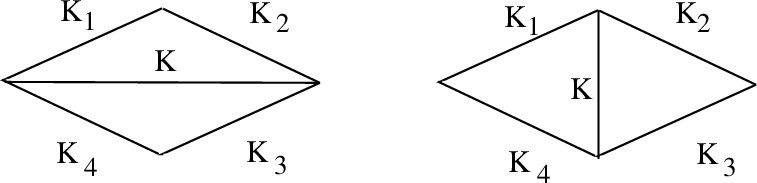
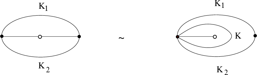
Identities between integral formulas resulting from cutting a general \({\Bbb S}\) follow formally from this.
Formulas (26 ) - (28 ) are similar to formulas in the classical theory of spherical functions [16]. The Hecke algebra of spherical functions is given by compactly supported functions on \({\rm SL}_2({\mathbb{R}})\), invariant under the left and right actions of \({\rm SO}(2)\), with the convolution product. It is a commutative algebra, and its characters are described by zonal spherical functions similarly to (28 ).
In our case Whittaker functions on \({\rm SL}_2({\mathbb{R}})\) play the role of spherical functions, covariant under the left and right action of the unipotent subgroup \({\rm N}({\mathbb{R}})\subset {\rm SL}_2({\mathbb{R}})\) by a given non-trivial character. The Bessel function \({\cal B}_{\rm T}({\rm K}, s)\) is the restriction of the zonal Whittaker function for the principal series representation \(V_s\) of \({\rm PGL}_2({\mathbb{R}})\) to the Cartan subgroup. The key difference is that the convolution of such functions is ill-defined due to non-compactness of \({\rm N}({\mathbb{R}})\). Remarkably, one can still define the product for restrictions of Whittaker functions to the positive diagonal matrices by formula (26 ). This suggests the name positive Whittaker–Hecke algebra for the algebra \({\cal E}\). We will continue the discussion in Section 8.
1.6 Exponential volumes are exponential periods↩︎
We show that the exponential volumes of moduli spaces are functions of algebraic-geometric origin. Here the space \({\cal P}_{\Bbb S}\) is essential, providing the complexification of the Teichmüller space, its volume form, and the potential \(W\).
We start with a data \[\label{DEM} (X, W, f, \Omega; \gamma),\tag{29}\] where \(X\) is a regular variety over \(\Bbb Q\), \(W\) and \(f\) is a regular function on \(X\), \(\Omega_X\) is an algebraic volume form on \(X\) with logarithmic singularities, and \(\gamma\) is a possibly non-compact cycle of real dimension \({\rm dim}(X)\) such that the map \(W:\gamma \to {\mathbb{C}}\) is proper, and \({\rm Re} \;W\to +\infty\). Then we can consider the following integral \[\label{ETI} \int_{\gamma\subset X({\mathbb{C}})}e^{-W} f \;\Omega_X.\tag{30}\] The conditions on the cycle \(\gamma\) guarantee that the integral is convergent: the integrand exponentially decays at infinity of the cycle \(\gamma\). The numbers which we can get this way are called the exponential periods over \({\mathbb{Q}}\). If the data (29 ) depends on parameters \({\rm K}\) parametrised by a variety \({\cal K}\), then the functions in \({\rm K}\) given by integrals (30 ) are called the periods of variations of exponential motives.
The exponential volume function \({\rm Vol}_{{\mathcal{E}}}\mathcal{M}_{\Bbb S}({{\rm K}}, {\rm L})\) is defined by an apparently similar data \[({\cal P}_{{\Bbb S}}, W, 1, \Omega_{\Bbb S}; \gamma={\cal T}^{\rm en}_{\Bbb S}).\] However this data is \({\rm Mod}({\Bbb S})-\)invariant. If the group \({\rm Mod}({\Bbb S})\) is finite, it defines an exponential period on the nose. Otherwise the integral diverges. So we have to integrate over a fundamental domain for the action of \({\rm Mod}({\Bbb S})\) on the Teichmüller space. Yet there is no natural choice of the fundamental domain.
Here is a classical analogy. It is known that for the standard invariant volume form \(\omega\) on \({\rm SL}_n\) we have \[\label{ZV} {\rm Volume}_\omega\Bigl({\rm SL}_n({\mathbb{R}})/{\rm SL}_n({\mathbb{Z}})\Bigr) := \int_{{\rm SL}_n({\mathbb{R}})/{\rm SL}_n({\mathbb{Z}})}\omega = \zeta(2) \zeta(3) \cdots \zeta(n).\tag{31}\] However it is not straightforward to give an algebraic-geometric interpretation of the volume. Yet its value is manifestly a mixed Tate period over \({\rm Spec}({\mathbb{Z}})\).
Theorem 8. The exponential volume \({\rm Vol}_{{\mathcal{E}}}\mathcal{M}_{\Bbb S}({{\rm K}}, {\rm L})\) is a period of a variation of exponential motives.
We give two proofs of Theorem 8, each providing an explicit way to write the exponential volume as a finite sum of exponential periods.
We calculate the \({\rm Vol}_{{\mathcal{E}}}\mathcal{M}_{\Bbb S}({{\rm K}}, {\rm L})\) using neck recursion formula (?? ) and Mirzakhani’s formula (6 ).
We apply unfolding formulas from Theorem 6 to calculate inductively the exponential volume \({\rm Vol}_{{\mathcal{E}}}\mathcal{M}_{\Bbb S}({{\rm K}}, {\rm L})\) as a finite sum of integrals of type (30 ).
Both proofs are based on different variants of unfolding in the Teichmüller theory.
Finally, we want to note the analogy between the Rankin-Selberg method in Number Theory and the unfolding in the Teichmüller theory.
1.6.1 Organization of the paper.↩︎
In Section 2 we prove the crucial cutting and gluing formulas for unfolding exponential volume forms.
In Section 2.1 we discuss the moduli space \({\cal P}_{{\Bbb S}}\) - the algebraic-geometric avatar of the Teichmüller space of ideal hyperbolic structures on \({\Bbb S}\), and recall the cluster Poisson coordinates \(\{{\rm B}_{\rm F}, X_{\rm E}\}\) on it assigned to an ideal triangulation of \({\Bbb S}\). Then we define the local potentials \({W}_p\) and the regular functions \({\rm K}_{\rm F}\) assigned to the boundary intervals of \({\Bbb S}\), and calculate them in the cluster Poisson coordinates. Restricting the functions \({\rm K}_{\rm F}\) to the positive locus we recover functions (1 ). After these preparations, we prove in Section 2.2 the cutting and gluing formulas for the exponential volume forms.
In Section 3 we calculate \({\cal B}-\)functions and prove Theorem 1 - the exponential volume is finite.
In Section 4 we prove Proposition 5 and use it to get the generalized McShane identity.
In Section 5 we prove Theorem 6 - the unfolding formula for the exponential volumes.
In Section 6 we study the tropicalization of exponential volumes, and prove that they are finite. In Section 6.3 we show that tropical volumes of spaces of measured laminations on punctured surfaces are equal to Kontsevich’s volumes, and so carry the same information as the intersection theory on \({\cal M}_{g,n}\).
In Section 7 we elaborate the simplest examples of the unfolding formula.
In Section 8 we show that exponential volumes for the elementary decorated surfaces with cusps describe a commutative associative algebra, which we call positive Whittaker–Hecke algebra for \({\rm PGL}_2({\mathbb{R}})\).
1.6.2 Acknowledgement.↩︎
We are very grateful to the referee for the terrific job. Essentially all referee’s comments and remarks are incorporated in the paper. This work was done at IHES during the Summer of 2023, and the final draft prepared during the Summer of 2024. We are grateful to IHES for the hospitality and support. The work of AG was supported by the NSF grants DMS-1900743 and DMS-2153059, and by the Gretchen and Barry Mazur Chair at IHES and the Simons Foundation fellowship in 2023.
2 Moduli spaces \(\mathcal{P}_{{\Bbb S}}\) and Teichmüller spaces↩︎
Given a group \({\rm G}\), recall the canonical equivalence of categories: \[\{{\em {\rm G}-local systems} {\cal L} on S\} \longrightarrow\{representations \rho: \pi_1(S,x) \to {\rm G} modulo the {\rm G}-conjugation\}.\] It assigns to a \({\rm G}-\)local system \({\cal L}\) on \(S\) the monodromy representation \(\rho: \pi_1(S, x) \longrightarrow{\rm G}\).
Now let \({\rm G}= {\rm PGL}_2\), and \({\cal B} :={\rm P}^1\). Let \({\rm {U}}\) be a maximal unipotent subgroup of \({\rm G}\), and \({\cal A}:={\rm G}/{\rm {U}}\) the decorated flag variety, which can be described as \[{\cal A} = \Bigr((V_2-\{0\}) \times ({\rm det} V_2^*-\{0\})\Bigr) /{\Bbb G}_m.\] Here \(V_2\) is a two-dimensional vector space. So the moduli space \({\cal A}\) parametrises pairs \((v, \omega)\) where \(v\) is a non-zero vector, and \(\omega\) an area form in \(V_2\), considered modulo the action of the multiplicative group \({\Bbb G}_m\): \[(v, \omega) \longrightarrow(\lambda v, \lambda^{-2}\omega).\] There is a canonical function \[\Delta: {\cal A} \times {\cal A} \longrightarrow{\rm A}^1, \qquad (v_1, \omega_1) \times (v_2, \omega_2) \longmapsto\omega_1(v_1, v_2)\omega_2(v_1, v_2).\] Given a \({\rm PGL}_2-\)bundle \({\cal L}\), let \({\cal L}_{{\rm P}^1}\) be the associated local system of projective lines, and \({\cal L}_{\cal A}\) the associated local system of two-dimensional vector bundles with area forms, modulo the action of the group \({\Bbb G}_m\).
Definition 5. [17]. Let \({\Bbb S}\) be a decorated surface. Let \({\cal L}\) be a \({\rm PGL}_2\)-local system on \({\Bbb S}\).
A framing* \({\cal L}\) at a puncture on \({\Bbb S}\) is a flat section of the associated local system \({\cal L}_{{\rm P}^1}\) near the puncture.*
The moduli space \(\mathcal{X}_{{\rm PGL}_2, {\Bbb S}} = \mathcal{X}_{{\Bbb S}}\) parametrises pairs \((\cal L, \beta)\), with a framing \(\beta\) at each puncture.
Here are better versions of the moduli space \(\mathcal{X}_{{\Bbb S}}\) for decorated surfaces \({\Bbb S}\) with marked boundary points, introduced and studied in [11] and [12]. Their key advantage is the existence of the gluing maps.
Definition 6. Let \({\Bbb S}\) be a decorated surface. Let \({\cal L}\) be a \({\rm PGL}_2\)-local system on \({\Bbb S}\).
A decoration* on \({\cal L}\) at a marked point \(p\) on \({\Bbb S}\) is a flat section of the associated local system \({\cal L}_{\cal A}\) near \(p\). We assume that the decorations at each pair of adjacent marked points are in generic position.*
The moduli space \({\cal P}_{{\rm PGL}_2, {\Bbb S}} = \mathcal{P}_{{\Bbb S}}\) parametrises triples \((\cal L, \alpha, \beta)\) where \(\cal L\) is a \({\rm PGL}_2\)-local system on \({\Bbb S}\) with a decoration \(\alpha\) at each marked point, and a framing \(\beta\) at each puncture.
The space \(\mathrm{Loc}_{{\rm PGL}_2,{\Bbb S}} = \mathrm{Loc}_{{\Bbb S}}\) parametrises pairs \(({\cal L}, {\alpha})\), with a decoration \(\alpha\) at each marked point.
So the moduli space \(\mathcal{P}_{{\Bbb S}}\) parametrises local systems of two-dimensional vector spaces on \({\Bbb S}\) with non-zero volume forms, modulo the action of \({\Bbb G}_m\), equipped with a flat section of the local system of lines near each puncture, and a pair \((v_p,\omega_p)\) at the fiber at each marked point \(p\), considered up to a common simultaneous rescaling in all fibers. The vectors \(v_{p}, v_{p'}\) at adjacent marked boundary points \(p, p'\) are in the generic position: their parallel transports to the middle of the segment \(p p'\) are not collinear. When the boundary component has a single marked point \(p\), the vector \(v_{p}\) is in generic position means that monodromy around the boundary component transforms \(v_p\) to a vector \(v_p'\) which is not collinear to \(v_p\).
Just like the space \(\mathcal{X}_{{\Bbb S}}\), the space \({\cal P}_{\Bbb S}\) is equipped with the action of the group \({\rm Mod}({\Bbb S})\), and carries a canonical \({\rm Mod}({\Bbb S})-\)equivariant cluster Poisson structure, given by an infinite collection of rational coordinate systems, related by cluster Poisson transformations, which we review in Section 2.1.
2.1 Cluster Poisson coordinates, local potentials, and the cluster volume form on \(\mathcal{P}_{{\Bbb S}}\)↩︎
2.1.1 Cluster Poisson coordinates on the space \(\mathcal{P}_{{\Bbb S}}\).↩︎
Given any local system on \({\Bbb S}\), its fiber over any simply-connected domain makes sense since the fibers at any two points of the domain are canonically isomorphic by parallel transport via a path in the domain connecting the points. In particular, we can talk about the fibers of the local system of projective lines \({\cal L}_{{\rm P}^1}\) over an edge, or over a rectangle of a triangulation of \({\Bbb S}\)
Pick a point \((\cal L, \alpha, \beta)\in \mathcal{P}_{{\Bbb S}}\). Take a boundary interval \({\rm F}\) with marked points \(p, p'\) at the ends. The decorations at the points \(p, p'\) can be viewed as decorations \((v_p, \omega_p), (v_{p'}, \omega_{p'})\) at the fiber of \({\cal L}\) at \({\rm F}\). We define the pinning point \(p_{{\rm F}}\) at the fiber of the local system \({\cal L}_{{\rm P}^1}\) at \({\rm F}\) as the projectivisation of the one dimensional subspace spanned by the following vector: \[\label{pli} p_{{\rm F}}:= \left\langle \omega_p(v_p, v_{p'})v_p + \omega_p(v_{p'}, v_{p})v_{p'} \right \rangle.\tag{32}\] So a point \((\cal L, \alpha, \beta)\in \mathcal{P}_{{\Bbb S}}\) provides the following distinguished points in the fibers of \({\cal L}_{{\rm P}^1}\):
A decoration point at the fiber over the marked point \(p\).
A pinning point at the fiber over the boundary edge \({\rm F}\).
A framing point at the fiber over a point near a puncture \(o\), invariant under the local monodromy.
Pick an ideal triangulation \({\cal T}\) of \({\Bbb S}\), that is a triangulation with the vertices at the marked points and punctures. It includes the collection of external edges given by the boundary segments of \({\Bbb S}\). The rest of the edges are the internal edges. Each edge \(\rm A\) of the triangulation gives rise to a rational function \[{\rm X}_{\rm A}: \mathcal{P}_{{\Bbb S}} \longrightarrow{\rm A}^1.\] It is defined as follows. If \(\rm E\) is an internal edge, there is a unique quadrilateral \(Q_{\rm E}\) containing \(\rm E\) as a diagonal. Let us denote its vertices by \(z_1, ..., z_4\), so that \(z_1\) is a vertex of the edge \(\rm E\), and the order of the points follows the orientation of the quadrilateral induced by the orientation of \({\Bbb S}\). Then we set \[{\rm X}_{\rm E}:= r(x_1,x_2,x_3, x_4):= \frac{\omega(\widetilde{x}_1, \widetilde{x}_2)\omega(\widetilde{x}_3, \widetilde{x}_4)}{\omega(\widetilde{x}_2, \widetilde{x}_3)\omega(\widetilde{x}_1, \widetilde{x}_4)}.\] where \(x_i\) is the distinguished point in the fiber of the local system \({\cal L}_{{\rm P}^1}\) at the point \(z_i\). To define the cross-ratio \(r(x_1,x_2,x_3,x_4)\), we parallel transform the points \(x_i\) to a center of the quadrilateral, and pick arbitrary non-zero vectors \(\widetilde{x}_i\) in the fiber projecting to the points \(x_i\), and use any area form \(\omega\) in the fiber. Then \({\rm X}_{\rm E}\) evidently does not depend on the choices.
If the edge \(\rm A\) is an external edge \({\rm F}\), there is a unique triangle \(t_{\rm F}\) of the triangulation with the base \({\rm F}\). Then there is a quadruple of distinguished points \((x_1, x_2, x_3, x_4)\), where \((x_1, x_3)\) are the decoration points at the vertices of \({\rm F}\), counted counterclockwise, \(x_2\) is the pinning point at the edge \({\rm F}\), and \(x_4\) is the framing/decoration point over the vertex of the triangle \(t\) which does not belong to \({\rm F}\). We define \({\rm X}_{\rm F}\) as the cross-ratio \[{\rm X}_{\rm F}:=r(x_1, x_2, x_3, x_4).\]
Definition 7. The boundary Poisson coordinates \({\rm B}_{{\rm F}}\) are assigned to the boundary edges \({\rm F}\) and given by \[{\rm B}_{{\rm F}}:= {\rm X}_{\rm F}.\]
Theorem 9. The collection of rational functions \(\{{\rm X}_{\rm E}, {\rm X}_{\rm F}\}\) assigned to the edges of an ideal triangulation of \({\Bbb S}\) provides a cluster Poisson structure on the space \(\mathcal{P}_{{\Bbb S}}\). The Poisson bracket is given by \[\label{FEPS} \{{\rm X}_{\rm A}, {\rm X}_{\rm B}\}= \varepsilon_{\rm A B}{\rm X}_{\rm A} {\rm X}_{\rm B}, \qquad \varepsilon_{{\rm A}\rm B} = -\varepsilon_{\rm B {\rm A}}\in {\mathbb{Z}}.\qquad{(10)}\]
The Poisson tensor \(\varepsilon_{{\rm A} {\rm B}}\) is defined by \(\varepsilon_{{\rm A} {\rm B}} := \sum_v \delta_{v}( {\rm A}, {\rm B}).\) The sum is over common vertices \(v\) of the edges \({\rm A}, {\rm B}\). We set \(\delta_v({\rm A} ,{\rm B})=0\) unless the edges \({\rm A}, {\rm B}\) are
adjacent. In the latter case, \(\delta_v({\rm A}, {\rm B}) =1\) if \({\rm B}\) is after \({\rm A}\) at the vertex \(v\)
following the (clockwise on the pictures) orientation of \({\Bbb S}\), and \(-1\) otherwise. Theorem 9 is proved in
Subsection 2.6 below.
Besides cluster Poisson coordinates, there are canonical functions \({\rm K}_{\rm F}\) at the boundary edges \({\rm F}\) of \({\Bbb S}\).
Definition 8. Let \((\omega_i, v_i)\) and \((\omega_{i+1}, v_{i+1})\) be the decorations at the ends of a boundary edge \({\rm F}\). Then the function \({\rm K}_{\rm F}\) assigned to the boundary edges \({\rm F}\) of \({\Bbb S}\) is given by \[{\rm K}_{\rm F}:=( \omega_i(v_i, v_{i+1})\omega_{i+1}(v_i, v_{i+1}))^{-1}.\]
The function \({\rm K}_{\rm F}\) does not depend on the choice of the orientation of the edge \(\rm F\).
Thanks to Definitions 6 and 8, we get a canonical regular non-zero function \[{\rm K}_{\rm F}: \mathcal{P}_{{\Bbb S}} \longrightarrow{\rm A}^1.\] More generally, given any edge \(\rm E\) connecting two cusps on \({\Bbb S}\), there is a rational function \(\rm {K}_{\rm E}\) on the space \({\cal P}_{{\rm PGL}_2, {\Bbb S}}\). Namely, let \((\omega_1, v_1)\) and \((\omega_2, v_2)\) be the decorations at the vertices \(v_1, v_2\) of the edge \({\rm E}\). Then \[{\rm {K}}_{\rm E}:= (\omega_1(v_1, v_2) \omega_2(v_1, v_2))^{-1}.\]
2.1.2 The potential function.↩︎
For each marked point \(p\) on \({\Bbb S}\), there is a function \(W_p\) on \(\mathcal{P}_{{\Bbb S}}\), called the potential at \(p\). It is defined as follows. Pick a non-zero volume form \(\omega\) at the fiber at the marked point \(p\). So the decorations at \(p\) are given by pairs \((v_p,\omega)\). Let us parallel transport the form \(\omega\) to nearby points on the boundary of \({\Bbb S}\) to the left and to the right of \(p\). Denote by \((v_-,\omega)\) and \((v_+,\omega)\) the decorations at the fibers of \({\cal L}\) at the marked points \(p_-\) and \(p_+\) to the left and to the right of \(p\). Then we define \[W_p({\cal L}, \alpha, \beta):= \frac{\omega(v_-, v_+)}{\omega(v_p, v_-) \omega(v_p, v_+)}.\]
The potential does not change if we multiply any of the two vectors \(v_-, v_+\) by a non-zero scalar.
The potential function also does not change under the equivalence \((v_p, \omega) \sim (\lambda v_p, \lambda^{-2}\omega)\).
Therefore the potential at \(p\) is a well defined non-vanishing regular function \[W_p: {\cal P}_{ {\Bbb S}}\longrightarrow{\rm A}^1.\] Indeed, vectors \(v_p, v_-, v_+\) are non-zero, and pairs of vectors \((v_p, v_-)\) and \((v_p, v_+)\) are not collinear.
Definition 9. The potential function \(W\) is the sum of the potentials at all marked points \(p\) of \({\Bbb S}\): \[W:= \sum_{p}W_p.\]
2.1.3 The cluster volume form and its sign.↩︎
The cluster volume form \(\Omega_{\Bbb S}\) is a volume form with logarithmic singularities on the moduli space \(\mathcal{P}_{{\Bbb S}}\). It is given by the product of the logarithmic 1-forms over all edges of a given ideal triangulation \({\cal T}\) of \({\Bbb S}\), defined up to a sign:5 \[\label{CVF} \Omega_{\Bbb S}:= \pm 2^{\pi_0({\Bbb S})} d\log {\rm X}_{\rm E_1} \wedge \ldots \wedge d\log {\rm X}_{{\rm E}_{k}}.\tag{33}\] The sign of \(\Omega_{\Bbb S}\) depends on the choice of an order of the edges.
We take care of the sign issue of (33 ) as follows. Denote by \({\cal E}_{\cal T}\) the set of the edges of an ideal triangulation \({\cal T}\) of \({\Bbb S}\). Let \({\rm Or}_{\cal T}\) be its orientation torsor. It is a \({\mathbb{Z}}/2{\mathbb{Z}}-\)torsor, that is a 2-element set equipped with the non-trivial \({\mathbb{Z}}/2{\mathbb{Z}}-\)action. Its elements are orderings of the set \({\cal E}_{\cal T}\) modulo even permutations. We denote the element corresponding to an ordering \({\rm E}_{i_1}, ...,{\rm E}_{i_{k}}\) by \[\varepsilon_{\cal T}(i_1, ..., i_{k}) \in {\rm Or}_{\cal T}.\] Given a flip of an ideal triangulation \(\varphi_{\rm E}: {\cal T} \longrightarrow{\cal T}'\) at an edge \({\rm E}\), there is a canonical identification of the edges of \({\cal T}\) and \({\cal T}'\). It gives rise to the following isomorphism of the orientation torsors \[\label{53} \begin{align} &\varphi_{\rm E}: {\rm Or}_{\cal T} \longrightarrow{\rm Or}_{\cal T'}, \\ &\varepsilon_{\cal T}(i_1, ..., i_{k})\longmapsto-\varepsilon_{\cal T'}(i_1, ..., i_{k}).\\ \end{align}\tag{34}\] Here \(-\) amounts to the action of the element \(-1 \in {\mathbb{Z}}/2{\mathbb{Z}}\). To state the properties of this construction, recall the modular groupoid \({\cal G}_{\Bbb S}\) of a decorated surface \({\Bbb S}\).
The modular groupoid \({\cal G}_{\Bbb S}\) is a groupoid whose objects are ideal triangulations \({\cal T}\) of \({\Bbb S}\), the morphisms are generated by the flips, and the relations between the flips are generated by
(i) Pentagon relations: the composition of the five flips of diagonals of a pentagon is the identity map.
(ii) Square relations: the flips at disjoint diagonals commute.
The mapping class group of \({\Bbb S}\) is the fundamental group of the modular groupoid. The proof is deduced from Strebel’s theory of quadratic differentials [18], [19], see [17] for further discussion.
Lemma 2. There is a functor from the groupoid \({\cal G}_{\Bbb S}\) to the groupoid of \({\mathbb{Z}}/2{\mathbb{Z}}-\)torsors, which assigns to an ideal triangulation \({\cal T}\) of \({\Bbb S}\) the \({\mathbb{Z}}/2{\mathbb{Z}}-\)torsor \({\rm Or}_{\cal T}\), and to a flip at an edge \({\rm E}\) the isomorphism (34 ).
Proof. We have to prove that the compositions of flips for the square and pentagon relations induce the identity maps on the orientation torsor. The composition of the five flips related to a pentagon returns back the original triangulation of the pentagon, but the order of the two internal diagonals is switched, which agrees with \((-1)^5=-1\). The diagonals outside of the pentagon remain intact. So the composition acts as the identity map on the orientation torsor. The square relations are evident. ◻
Since all orientation torsors \({\rm Or}_{\cal T}\) are canonically isomorphic, and the isomorphisms between them are compatible with the relations, we arrive at the canonical orientation torsor \({\rm Or}_{{\Bbb S}}\) assigned to a decorated surface \({\Bbb S}\). It allows us to introduce the cluster volume form with values in the tensor product of the volume forms with logarithmic singularities on \({\cal P}_{\Bbb S}\) by the orientation torsor: \[\label{CVF+} \Omega_{\Bbb S}\in {\rm Or}_{{\Bbb S}} \otimes_{{\mathbb{Z}}/2{\mathbb{Z}}} \Omega_{\rm log}({\cal P}_{\Bbb S}).\tag{35}\] Here the group \({\mathbb{Z}}/2{\mathbb{Z}}\) acts on volume forms so that the generator acts by changing the sign of the form.
Definition 10. The cluster volume form \(\Omega_{\Bbb S}\) in (35 ) is given by setting \[\label{CVF***} \begin{align} &\Omega_{\Bbb S}:= 2^{\pi_0({\Bbb S})} \cdot \varepsilon_{\cal T}(i_1, ..., i_{k}) \otimes_{{\mathbb{Z}}/2{\mathbb{Z}}} d\log {\rm X}_{\rm E_1} \wedge \ldots \wedge d\log {\rm X}_{{\rm E}_{k}}.\\ \end{align}\qquad{(11)}\]
The crucial fact that the cluster volume form does not depend on the choice of an ideal triangulation \({\cal T}\) is easy to check directly. It can also be deduced from the general properties of the cluster volume form on cluster varieties, which we address in the next subsection, see Lemma 3.
2.1.4 The canonical cluster volume form on a cluster variety.↩︎
We address the reader to [3] for general properties of cluster varieties. The above construction, suitably modified, provides the cluster volume form on any cluster variety. Namely, given a seed \({\boldsymbol{c}}\), we introduce the orientation \({\mathbb{Z}}/2{\mathbb{Z}}-\)torsor \({\rm Or}_{\boldsymbol{c}}\). Its elements \(\varepsilon_{\boldsymbol{c}}(i_1, ..., i_{k})\) correspond to the ordered cluster coordinates \(({\rm X}_{i_1}, ..., {\rm X}_{i_k})\) in the seed \({\boldsymbol{c}}\). Interchanging two coordinates amounts to changing the sign. A mutation \(\mu_k: {\boldsymbol{c}} \longrightarrow{\boldsymbol{c}}'\) gives rise to a canonical isomorphism of \({\mathbb{Z}}/2{\mathbb{Z}}-\)torsors \[\label{CICS} \begin{align} &\mu_{k}: {\rm Or}_{\boldsymbol{c}} \longrightarrow{\rm Or}_{\boldsymbol{c}'}, \\ &\varepsilon_{\boldsymbol{c}}(i_1, ..., i_{k})\longmapsto-\varepsilon_{\boldsymbol{c}'}(i_1, ..., i_{k}).\\ \end{align}\tag{36}\] These isomorphisms satisfy the standard \((h+2)-\)gon relations, discussed in [3], which are used to introduce the cluster modular groupoid. If the quiver underlying the seed \({\boldsymbol{c}}\) is simply-laced, then \(h=2,3\). Moreover, for the cluster variety \({\cal P}_{\Bbb S}\) we recover the square and pentagon relations. So we arrive at the \({\mathbb{Z}}/2{\mathbb{Z}}-\)torsor \({\rm Or}_{\cal X}\).
The group \({\mathbb{Z}}/2{\mathbb{Z}}\) acts on volume forms so that the generator acts by changing the sign of the form. Then the cluster volume form on a cluster Poisson variety \({\cal X}\) is defined by \[\label{CVF*} \begin{align} & \Omega_{\cal X}\in {\rm Or}_{\cal X} \otimes_{{\mathbb{Z}}/2{\mathbb{Z}}} \Omega_{\rm log}({\cal X}); \\ &\Omega_{\cal X}:= \varepsilon_{\boldsymbol{c}}(i_1, ..., i_{k}) \otimes_{{\mathbb{Z}}/2{\mathbb{Z}}} d\log {\rm X}_{i_1} \wedge \ldots \wedge d\log {\rm X}_{i_k}. \\ \end{align}\tag{37}\] It evidently does not depend on the choice of the order of the cluster coordinates.
Similarly, the cluster volume form on a cluster \({\cal A}-\)variety \({\cal A}\) is given by \[\label{CVF*A} \begin{align} & \Omega_{\cal A}\in {\rm Or}_{\cal A} \otimes_{{\mathbb{Z}}/2{\mathbb{Z}}} \Omega_{\rm log}({\cal A}); \\ &\Omega_{\cal A}:= \varepsilon_{\boldsymbol{c}}(i_1, ..., i_{k}) \otimes_{{\mathbb{Z}}/2{\mathbb{Z}}} d\log {\rm A}_{i_1} \wedge \ldots \wedge d\log {\rm A}_{i_k}. \\ \end{align}\tag{38}\]
Remark 10. The cluster volume form \(\Omega_{\Bbb S}\) on the space \({\cal P}_{\Bbb S}\) introduced in (?? ) is equal to \(2^{\pi_0({\Bbb S})}\) times the cluster volume form \(\Omega_{\cal X}\) on the related cluster variety. Due to the extra factor \(2^{\pi_0({\Bbb S})}\) we get simpler constants in unfolding formulas, including the constant \(1\) in the cutting formulas (?? ) and (?? ).
Lemma 3. The cluster volume forms \(\Omega_{\cal X}\) and \({\Omega}_{\cal A}\) are invariant under cluster mutations.
Proof. i) The cluster Poisson mutation \(\mu_{k}\) acts by \({\rm X}_k \longmapsto{\rm X}_k^{-1}\) and \({\rm X}_j \longmapsto{\rm X}_j P_j({\rm X}_k)\), \(j \not = k\), where \(P_j({\rm X}_k)\) is a Laurent polynomial in \({\rm X}_k\), see [3]. Therefore it changes the sign of the form \(d\log {\rm X}_{i_1} \wedge \ldots \wedge d\log {\rm X}_{i_n}\). This sign change is compensated by the sign change in isomorphism (36 ).
ii) The proof in the \({\cal A}-\)case is similar. The only cluster coordinate which changes under the mutation \(\mu_k\) is the one \({\rm A}_k\), and the exchange relation tells that \({\rm A}_k{\rm A}_k'\) is a Laurent polynomial in \({\rm A}_j\) where \(j \not = k\). Therefore the form \(d\log {\rm A}_{i_1} \wedge \ldots \wedge d\log {\rm A}_{i_n}\) changes sign under mutations. ◻
Proposition 11. The cluster volume form \(\Omega_{\cal X}\) induces a canonical positive measure \(\Omega_{\cal X}\) on the space of positive real points \({\cal X}({\mathbb{R}}_{>0})\). The same is true for the cluster \({\cal A}-\)varieties.
Proof. Given a seed \({\boldsymbol{c}}\), the cluster coordinates provide a canonical isomorphism \[i_{\boldsymbol{c}}: {\cal X}({\mathbb{R}}_{>0}) \longrightarrow{\mathbb{R}}^k.\] Therefore an order of the cluster coordinates provides an orientation of the space \({\cal X}({\mathbb{R}}_{>0})\). Altering the order we alter the orientation by the sign of the permutation. The same sign shows up in the cluster volume form. So the integral of the cluster volume form over a compact domain is positive. ◻
2.1.5 Calculating the potential and \({\rm K}-\)functions.↩︎
Take a vertex \(v\) of an ideal triangulation \({\cal T}\) of \({\Bbb S}\). The orientation of \({\Bbb S}\) provides the counterclockwise orientation of the edges of \({\cal T}\) sharing the vertex \(v\).
Theorem 12. Denote by \({{\rm F}}, {\rm E_1}, ..., {\rm E_k}, {{\rm F}^+}\) the edges sharing a vertex \(v\) of the triangulation \({\cal T}\), ordered counterclockwise. So \({\rm F}, {\rm F}^+\) are the two external edges sharing the vertex \(v\), which may coincide.
Then the function \({\rm K}_{\rm F}\) and the potential \(W_v\) are given by: \[\label{kf} { \rm K}_{{\rm F}^+}= {\rm B}_{{\rm F}}{\rm X}_{\rm E_1} \ldots {\rm X}_{\rm E_k} {\rm B}_{{\rm F}^+}.\qquad{(12)}\] \[\label{fw} W_v = {\rm B}_{{\rm F}} + {\rm B}_{\rm F}{\rm X}_{{\rm E}_1} + \ldots + {\rm B}_{\rm F}{\rm X}_{{\rm E}_1} \ldots {\rm X}_{{\rm E}_{k}}.\qquad{(13)}\]
Proof. This is done by an explicit calculation. We start from the two simplest examples of the calculation.
2.1.6 The triangle.↩︎
Let \({\Bbb S}=\tau\) be a triangle. Denote by \((v_i,\omega)\) a decoration at the vertex \(i\), where \(i={\mathbb{Z}}/3{\mathbb{Z}}\), and the vertices are numbered counterclockwise. Here \(v_i\) are non-zero vectors in a two dimensional vector space \(V_2\). There is a unique vector \(v_{i+1}'\) proportional to \(v_{i+1}\) such that \(\omega(v_i, v'_{i+1})=1\), see Figure 11: \[v_{i+1}'= \frac{v_{i+1}}{\omega(v_i, v_{i+1})}.\]
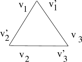
So the pinning vector on the side \((i, i+1)\) of the triangle is given by \[p_{i, i+1}= v_i+v'_{i+1}.\] Therefore the \({\rm B}-\)coordinate assigned to the side \((i, i+1)\) is \[{\rm B}_{i, i+1}:= r^+(v_i, p_{i, i+1}, v_{i+1}, v_{i+2}) = \frac{\omega(v_{i+1}, v_{i+2})}{\omega(v_{i}, v_{i+1})\omega(v_{i}, v_{i+2})}.\] This coincides with the potential \(W_{i}\) at the vertex \(i\), see [12], confirming (?? ): \[\label{FPo} W_{i} = {\rm B}_{i, i+1}.\tag{39}\] Finally, we have the following, confirming formula (?? ): \[{\rm B}_{12}{\rm B}_{31}= \frac{\omega(v_{2}, v_{3})}{\omega(v_{1}, v_{2})\omega(v_{1}, v_{3})} \cdot \frac{\omega(v_{1}, v_{2})}{\omega(v_{3}, v_{1})\omega(v_{3}, v_{2})} = \omega(v_1, v_3)^{-2}.\]
2.1.6.1 The rectangle.
Let \({\Bbb S}\) be a rectangle with decorations \((\omega, v_i)\) at the vertex \(i\), where \(i={\mathbb{Z}}/4{\mathbb{Z}}\). Let \({\rm E}\) be the internal diagonal connecting vertices \(1\) and \(3\).
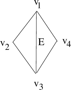
Denote the potential at the vertex \(1\) of the oriented angle \(314\) by \[\label{PEVE} W_{1}((1,3), (1,4)):=W_{314}:=\frac{\omega(v_3, v_4)}{\omega(v_1, v_3) \omega(v_1, v_4)},\tag{40}\] etc. Note that \(W_{413}=-W_{314}\). Then \[{\rm B}_{23} = W_2, \;\;\;{\rm B}_{41} = W_4, \;\;\;{\rm B}_{12}= W_{213}, \;\;\;{\rm B}_{34}= W_{431}.\] Calculation shows that \[{\rm X}_{\rm E} = \frac{W_{314}}{{\rm B}_{12}}.\] Therefore we have, using the additivity of the potential, and confirming formula (?? ): \[W_1 = W_{213} + W_{314} = {\rm B}_{12}+ {\rm B}_{12}{\rm X}_{\rm E}.\]
Finally, we have the following, confirming formula (?? ): \[{\rm K}_{41} = {\rm B}_{12}{\rm X}_{\rm E} {\rm B}_{41}= \frac{\omega(v_{2}, v_{3})}{\omega(v_{1}, v_{2})\omega(v_{1}, v_{3})} \cdot \frac{\omega(v_{1}, v_{2})\omega(v_{3}, v_{4})}{\omega(v_{2}, v_{3})\omega(v_{1}, v_{4})}\cdot \frac{\omega(v_{1}, v_{3})}{\omega(v_{4}, v_{1})\omega(v_{4}, v_{3})}= \omega(v_1,v_4)^{-2}.\] The case of an \(n-\)gon is very similar, and the general case reduces to this. ◻
We conclude that the moduli space \(\mathcal{P}_{ {\Bbb S}}\) carries functions of three flavors:
The regular functions \({\rm K}_{{\rm F}}\) assigned to the external edges \({\rm F}\) on \({\Bbb S}\).
The rational functions \({{\rm B}}_{{\rm F}}\) assigned to the external edges \({\rm F}\) on \({\Bbb S}\).
The rational functions \({{\rm X}}_{\rm E}\) assigned to the internal edges \(\rm E\) of a given ideal triangulation of \({\Bbb S}\).
The regular potential functions \(W_p\) assigned to the marked boundary points \(p\).
These functions are related by the relations (?? ) and (?? ).
::: {#PropP=X .proposition} Proposition 13. There is a canonical isomorphism \[\label{P=Xa} \mathcal{P}_{{\Bbb S}} = \mathcal{X}_{{\Bbb S}'}\qquad{(14)}\] where the decorated surface \({\Bbb S}'\) is obtained from \({\Bbb S}\) by adding a marked point inside each boundary interval. :::
Proof. Any \(({\cal L}, \alpha, \beta)\in \mathcal{P}_{{\Bbb S}}\) gives rise to a pinning point \(p_{\rm F}\) in the fiber of the local system \({\cal L}_{{\rm P}^1}\) over each boundary interval \({\rm F}\), see (32 ). So we get a point of \(\mathcal{X}_{{\Bbb S}'}\) given by the local system \({\cal L}\) together with the pinning points \(p_{\rm F}\) and the framing points.
Conversely, take the three framing lines \({\rm L}_p, {\rm L}_{\rm F}, {\rm L}_q\subset V_2\) at the ends \(p, q\) of a boundary interval \({\rm F}\) and at \({\rm F}\). Then \({\rm L}_{\rm F}\) is the graph of an isomorphism \(i_{\rm F}: {\rm L}_p\longrightarrow{\rm L}_q\). There exist decorating pairs \((v_p,\omega_p)\) and \((v_q,\omega_q)\) at the vertices \(p,q\) such that \[\label{Co} \omega_p(v_p, v_q) \omega_q(v_p, v_q)=1, \qquad v_q = i_{\rm F}(v_p).\tag{41}\] The pair \((v_p,\omega_p)\), and hence \((v_q,\omega_q)\), are defined uniquely up to rescaling. Indeed, if \(v'_p:= \lambda v_p\), then \(v_q'=\lambda v_q\). So there is a unique up to a sign \(\lambda\in \Bbb C^\times\) such that equation (41 ) holds. Note that \((-v_p,\omega_p)\) is obtained by rescaling of \((v_p,\omega_p)\) by \(-1\). We declare these \((v_p,\omega_p)\) and \((v_q,\omega_q)\) the decorations at the marked point \(p\) and \(q\). So the framing lines \(\{{\rm L}_p\}\) at the marked points \(p\) and the pinning lines \(\{{\rm L}_{\rm F}\}\) at the boundary edges \({\rm F}\) determine uniquely the decorations \((v_p, \omega_p)\) at the marked points \(p\). ◻
2.1.7 Proof of Theorem 9.↩︎
The mapping class group equivariant cluster Poisson structure on \(\mathcal{X}_{G,{\Bbb S}'}\) was defined in [17]. It is the one constructed in Theorem 9.
2.1.8 The enhanced Teichmüller space \({\cal T}^{\rm en}_{\Bbb S}\) is the set of real positive points of \({\cal P}_{ {\Bbb S}}\).↩︎
The enhanced Teichmüller space \({\cal T}_{\Bbb S}^e\) is the \(2^{m-r}:1\) ramified cover of the Teichmüller space \({\cal T}_{\Bbb S}\), parametrising ideal hyperbolic structures on \({\Bbb S}\) with a choice of a sign of the length of geodesic around each puncture.
::: {#P=X .theorem} Theorem 14. The enhanced Teichmüller space \({\cal T}^{\rm en}_{\Bbb S}\) of a decorated surface \({\Bbb S}\) is canonically isomorphic to the space of real positive points of the cluster Poisson variety \({\cal P}_{{\Bbb S}}\): \[{\cal T}^{\rm en}_{\Bbb S}= {\cal P}_{ {\Bbb S}}({\mathbb{R}}_{>0}).\] :::
Proof. Proposition 13 reduces the claim to the description of positive real locus of the space \(\mathcal{X}_{{\Bbb S}'}\). According to [17], we have \(\mathcal{X}_{{\Bbb S}'}({\mathbb{R}}_{>0}) = {\cal T}^{\rm en}_{{\Bbb S}'}.\) On the other hand, we have \(\mathcal{X}_{{\Bbb S}'}({\mathbb{R}}_{>0}) = \mathcal{P}_{{\Bbb S}}({\mathbb{R}}_{>0}).\) ◻
The cluster Poisson coordinates of an ideal triangulation of \({\Bbb S}\) provide an isomorphism \(\mathcal{T}^{en}_{\Bbb S}\stackrel{\sim}{\longrightarrow} {\mathbb{R}}_{>0}^N.\)
Lemma 4. The cluster volume form \(\Omega_{\Bbb S}\) in (35 ) gives rise to a positive measure on the enhanced Teichmüller space \({\cal T}^{\rm en}_{{\Bbb S}}\).
Proof. Ordering the edges of an ideal triangulation \({\cal T}\) of \({\Bbb S}\) we get the sign of the form \(\Omega_{\Bbb S}\) as well as an orientation of the enhanced Teichmüller space \({\cal T}^{\rm en}_{{\Bbb S}}\). Changing the order of the edges we change simulteneously the sign of the volume form and the orientation of the enhanced Teichmüller space. So the restriction of the form \(\Omega\) to the enhanced Teichmüller space provides canonical measure on it. ◻
Therefore for any continuous function \(f\) on the Teichmüller space, and any compact domain \({\cal D}\), the integral \(\int_{\cal D} f\Omega_{\Bbb S}\) makes sense. If \(f\) is a positive function, the integral is positive.
2.2 The cutting and gluing maps for the moduli spaces \({\cal P}_{\Bbb S}\)↩︎
2.2.1 The gluing map.↩︎
Take a decorated surface \({\Bbb S}'\), possibly disconnected. Let us glue edges \(\rm {E}'\) and \({\rm E}''\) on \({\Bbb S}'\) into an edge \(\rm E\) on \({\Bbb S}\), getting a new decorated surface \({\Bbb S}\). Denote by \({\cal P}_{{\Bbb S}'}^\delta\) the subspace of \({\cal P}_{{\Bbb S}'}\) defined by the equation \(\rm {K}_{{\rm E}'} = \rm {K}_{{\rm E}''}\). Then there is a gluing map [12]: \[\label{GM} \gamma_{{\rm E}' {\rm E}''}: {\cal P}^\delta_{ {\Bbb S}'} \longrightarrow{\cal P}_{ {\Bbb S}}.\tag{42}\] Namely, take a point \(({\cal L}, \alpha, \beta)\in {\cal P}^\delta_{ {\Bbb S}'}\). Then we can glue uniquely the \({\rm PGL}_2-\)local system \({\cal L}\) on \({\Bbb S}'\) to a local system onto \({\Bbb S}\) so that the decorations at the vertices \(x'_i, x''_i\) on \({\Bbb S}'\) matching the vertex \(x_i\) on \({\Bbb S}\) produce decorations at the vertices \(x_i\) on \({\Bbb S}\), for \(i=1,2\). Indeed, take the decoration vectors \(v'_1, v'_2\) on \({\rm E}'\) and \(v_1'', v_2''\) on \({\rm E}''\). Since \(\rm {K}_{{\rm E}'} = \rm {K}_{{\rm E}''}\not = 0\), we have \(\omega(v_1', v_2') = \pm \omega(v_1'', v_2'') \not = 0\). So there is a unique up to multiplication by \(-1\) isomorphism of vector spaces \[\varphi: {\cal L}'_{| \rm E'}\longrightarrow{\cal L}'_{|\rm E''}\] such that \(\varphi(v_i')= v_i''\). Note that decorations \((v,\omega)\) and \((-v, \omega)\) are the same by the definition.
The gluing map acts on cluster Poisson coordinates as follows. Take an ideal triangulation of \({\Bbb S}'\). It provides an ideal triangulation of \({\Bbb S}\). Let \({\rm B}', {\rm B}'', {\rm X}\) be the cluster Poisson coordinates assigned to the edges \(\rm {E}', \rm {E}'', {\rm E}\). By [12], we have \[\label{BB} \gamma_{{\rm E}' {\rm E}''}^*({\rm X}) = {\rm B}'{\rm B}''.\tag{43}\] The map \(\gamma_{{\rm E}' {\rm E}''}^*\) does not change the other coordinates.
2.2.2 The cutting map.↩︎
Take a decorated surface \({\Bbb S}\) with an internal edge \(\rm E\) connecting marked points. Denote by \({\Bbb S}'\) the decorated surface obtained by cutting \({\Bbb S}\) along \(\rm E\). It has two new boundary edges \({\rm E}'\), \({\rm E}''\). We define a rational map \({\cal P}_{{\Bbb S}} \longrightarrow{\cal P}_{{\Bbb S}'}\) by restricting a local system on \({\Bbb S}\) to \({\Bbb S}'\), and inducing the decorations and framing. It is well defined if and only if the decoration lines at the ends of the edge \({\rm E}\), parallel transported to a point of \({\rm E}\) along the edge, are different. Its image lies in the subspace \({\cal P}^\delta_{{\Bbb S}'}\), defined by the equations \({\rm K}_{\rm E'}={\rm K}_{{\rm E}''}\not = 0\). So we arrive at the rational cutting map \[\label{cut2} {\rm cut}_{\rm E}: {\cal P}_{{\Bbb S}} \longrightarrow{\cal P}^\delta_{{\Bbb S}'}.\tag{44}\]
Lemma 5. The cutting and gluing maps \({\rm cut}_{\rm E}\) and \(\gamma_{{\rm E}' {\rm E}''}\) are mutually inverse birational isomorphisms.
Proof. Follows from the very definitions. ◻
2.2.3 Relative volume forms.↩︎
Consider a map assigning to a point of \({\cal P}_{\Bbb S}\) the collection of its \({\rm K}-\)coordinates: \[\label{bs} \begin{gather} \xymatrix{ b_{\Bbb S}: {\cal P}_{{\Bbb S}} \ar[r]^{}& {\cal K}_{{\Bbb S}}} := {\Bbb G}_m^{\{boundary intervals of {\Bbb S}\}}. \end{gather}\tag{45}\] There is a similar map for the surface \({\Bbb S}'\), where the projection to the first factor is given by \({\rm K}_{\rm E'}={\rm K}_{\rm E''}\): \[\label{bs75} \begin{gather} \xymatrix{ b^\delta_{{\Bbb S}'}: {\cal P}^\delta_{{\Bbb S}'} \ar[r]^{}& {\cal K}^\delta_{{\Bbb S}'}} = {\Bbb G}_m\times { {\Bbb G}_m}^{\{boundary intervals of {\Bbb S}\}}. \end{gather}\tag{46}\]
The volume form \(\Omega_{\Bbb S}\) together with the product of the canonical invariant volume forms \(d\log {\rm K}\) on \({\Bbb G}_m\) induce a volume form on the fibers of projection (45 ), denoted by \(\Omega_{\Bbb S}({\rm K})=\Omega_{\Bbb S}({\rm K}_1,...,{\rm K}_b)\), and defined up to a sign from the equation:6 \[\label{RVF} d\log {\rm K}_1 \wedge \ldots \wedge d\log {\rm K}_b \wedge \Omega_{\Bbb S}({\rm K}) = \Omega_{\Bbb S}.\tag{47}\] Here \(b\) is the number of boundary edges on \({\Bbb S}\). The sign is determined by an order of the set of boundary edges, modulo even permutations. Similarly, we get a form \(\Omega^\delta_{{\Bbb S}'}({\rm K})\) on the fibers of projection (46 ). More generally, we define \(\Omega_{\Bbb S}({\rm K},{\rm L})\) such that \[\label{RVF2} d\log {\rm K}_1 \wedge \ldots \wedge d\log {\rm K}_b \wedge d l_1\wedge \ldots\wedge d l_a \wedge \Omega_{\Bbb S}({\rm K},{\rm L}) = \Omega_{\Bbb S}.\tag{48}\] where \({\rm L}=(l_1,...,l_a)\) are the boundary geodesic circle lengths.
Before we proceed with the proof, let us make some preparations.
The gluing map is described nicely in the cluster Poisson coordinates \(({\rm B}, X)\) in (43 ). The relative volume form \(\Omega_{\Bbb S}({\rm K})\) is defined in (47 ) by dividing the cluster volume form \(\Omega_{\Bbb S}\), expressed nicely in the cluster Poisson coordinates \(({\rm B}, X)\), by the volume form on the frozen torus, defined via \({\rm K}-\)coordinates.
The surface \({\Bbb S}'\) has two new boundary edges \({\rm E}'\) and \({\rm E}''\). We have the gluing condition: \[\label{KEEK} {\rm K}_{\rm E'}={\rm K}_{\rm E''} ={\rm K}_{\rm E}.\tag{49}\]
Pick an ideal triangulation of \({\Bbb S}\) containing the edge \({\rm E}\). It induces a triangulation of \({\Bbb S}'\). There is a unique vertex \(v_1'\) of \({\rm E}'\) such that \({\rm E}'\) is the last among the edges sharing \(v_1'\) in the counterclockwise order. There is a vertex \(v_2'\) of \({\rm E}''\) with the same property. Denote by \({\rm F}', {\rm E}'_{1}, ... {\rm E}'_{a}, {\rm E}'\) (respectively \({\rm F}'', {\rm E}''_{1}, ...,{\rm E}''_b, {\rm E}''\)) the edges sharing the vertex \(v_1'\) (respectively \(v_2'\)) on \({\Bbb S}'\), counted counterclockwise. Then we have the following monomial relations: \[\label{72} \begin{align} &{\rm K}_{\rm E'} \stackrel{ (\ref{kf})}{=} {\rm B}_{\rm F'} {\rm X}_{ {\rm E}'_{1}} \ldots {\rm X}_{ {\rm E}'_{a}}{\rm B}_{\rm E'},\\ &{\rm K}_{\rm E''} \stackrel{ (\ref{kf})}{=} {\rm B}_{\rm F''}{\rm X}_{ {\rm E}''_{1}} \ldots {\rm X}_{ {\rm E}''_{b}} {\rm B}_{\rm E''} ,\\ &{\rm X}_{\rm E} \stackrel{(\ref{BB})}{=}{\rm B}_{\rm E'} {\rm B}_{\rm E''}. \\ \end{align}\tag{50}\]
Now we return to the proof. Let us determine how the volume forms behave under cutting of an edge. We set, using the logarithmic coordinates \(dk_*:= d\log {\rm K}_*\):7 \[\Omega^\delta_{{\Bbb S}'}:=\delta(k_{{\rm E}'}- k_{{\rm E}''}) \Omega_{{\Bbb S}'}.\]
Lemma 6. Cutting a decorated surface \({\Bbb S}\) along an edge \({\rm E}\), we get \[\label{ECab} \begin{align} & \Omega_{\Bbb S}= {\rm cut}^*_{\rm E} \;\Omega^\delta_{{\Bbb S}'} \end{align}\qquad{(15)}\]

Proof. When \({\rm E}\) is separating as in Figure 13 (1), let \(k', k'', b', b''\) be the logarithmic \({\rm K}\) and \({\rm B}\) coordinates for the edges \({\rm E}'\) and \({\rm E}''\) on \({\Bbb S}'\), and \(x_{\rm E}\) the logarithmic \(x-\)coordinate at the edge \({\rm E}\). Then, see (50 ): \[x_{\rm E}= b'+b'', \;\;k'= b'+\ldots , \;\;\; k''= b'' + \ldots .\] Here \(\ldots\) stands for a sum of certain coordinates \(b_i\) and \(x_j\). The gluing condition is \[0= k'-k'' = b'-b'' + \ldots .\] Since \(x_{\rm E}= b' + b''\), we have \[\begin{align} & \Omega_{\Bbb S}= d x_{\rm E}\wedge i_{\partial/\partial x_{\rm E}} \Omega_{\Bbb S}=2d b' \wedge i_{\partial/\partial x_{\rm E}} \Omega_{\Bbb S}, \\ & \frac{1}{2} \Omega_{{\Bbb S}'} = db' db'' \wedge i_{\partial /\partial x_{\rm E}} \Omega_{\Bbb S},\\ & \Omega_{{\Bbb S}'} =2 d(k'-k'')\wedge db' \wedge i_{\partial /\partial x_{\rm E}} \Omega_{\Bbb S}=d(k'-k'')\wedge \Omega_{\Bbb S}.\\ \end{align}\] The lemma follows from this.
When \({\rm E}\) is non-separating as in Figure 13 (2), we have \[x_{\rm E}= b'+b'', \;\;k'= b'+\ldots , \;\;\; k''= b'+b'' + \ldots .\] Then the gluing condition is \[0=k'-k''=-b''+...\] Thus we get \[\begin{align} & \Omega_{\Bbb S}= d x_{\rm E}\wedge i_{\partial/\partial x_{\rm E}} \Omega_{\Bbb S}=d b' \wedge i_{\partial/\partial x_{\rm E}} \Omega_{\Bbb S}, \\ & \Omega_{{\Bbb S}'} = db' db'' \wedge i_{\partial /\partial x_{\rm E}} \Omega_{\Bbb S},\\ & \Omega_{{\Bbb S}'} =d(k'-k'')\wedge db' \wedge i_{\partial /\partial x_{\rm E}} \Omega_{\Bbb S}=d(k'-k'')\wedge \Omega_{\Bbb S}.\\ \end{align}\] ◻
We introduce the relative form \(\Omega^\delta_{{\Bbb S}'}({\rm K}_{\rm E})\), so that8 \[\Omega^\delta_{{\Bbb S}'}=\Omega^\delta_{{\Bbb S}'}({\rm K}_{\rm E}) \wedge d\log {\rm K}_{\rm E}.\] Formula (?? ) implies the key relation: \[\label{ECa} \begin{align} & \Omega_{\Bbb S}= {\rm cut}^*_{\rm E} \;\Omega^\delta_{{\Bbb S}'}({\rm K}_{\rm E}) \wedge d\log {\rm K}_{\rm E}. \end{align}\tag{51}\]
Proposition 15. Let \({\rm K}=({\rm K}_a)_a\) for all the boundary intervals. One has \[\label{EC} \begin{align} & \Omega_{\Bbb S}({\rm K}) = {\rm cut}^*_{\rm E} \;\Omega^\delta_{{\Bbb S}'}({\rm K}_{\rm E},{\rm K}) \wedge d\log {\rm K}_{\rm E}. \end{align}\qquad{(16)}\]
Proof. To calculate the form \(\Omega_{\Bbb S}({\rm K})\), we take the form \(\Omega_{\Bbb S}\), then divide it by the product of \(d\log {\rm K}_a\) for all boundary intervals on \({\Bbb S}\), and restrict to the fiber where \({\rm K}_a\)’s are constants. To calculate \(\Omega^\delta_{{\Bbb S}'}({\rm K})\) we have to do exactly the same. ◻
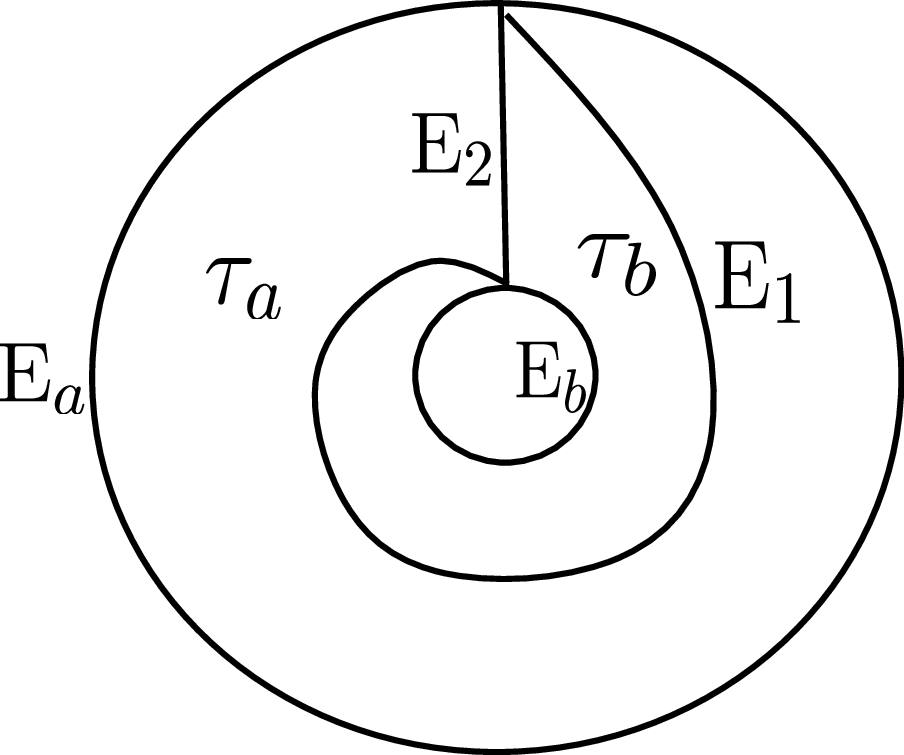
2.2.3.1 An example: \({\Bbb S}= {\rm A}_{1,1}\).
The annulus \({\rm A}_{1,1}\) is glued from two triangles \(\tau_a\) and \(\tau_b\) with the sides \({\rm E}_1^{(a)}, {\rm E}_2^{(a)}, {\rm E}_{a}\) and \({\rm E}_1^{(b)}, {\rm E}_2^{(b)}, {\rm E}_{b}\) respectively as in Figure 14. The logarithmic coordinates on the triangle \(\tau_a\) are \({b}_1^{(a)}, {b}_2^{(a)}, {b}_{a}\) and \({k}_1^{(a)}, {k}_2^{(a)}, {k}_{a}\), and similarly for the triangle \(\tau_b\). The relations are \[\begin{align} & {b}_1^{(a)} + {b}_2^{(a)} = {k}_1^{(a)}, \;\; {b}_2^{(a)} +{b}_a = {k}_2^{(a)}, \;\;\; {b}_a +{b}_1^{(a)} = {k}_a.\\ &{b}_1^{(b)} + {b}_2^{(b)} = {k}_1^{(b)}, \;\;\; {b}_2^{(b)}+ {b}_b = {k}_2^{(b)}, \;\;\; \;{b}_b +{b}_1^{(b)} = {k}_b.\\ \end{align}\] From this we calculate the relative forms on the triangles, which are just numbers: \[\Omega_{\tau_a}({\rm K}_a, {{\rm K}}_1^{(a)}, {{\rm K}}_2^{(a)})= 1, \;\;\; \Omega_{\tau_b}({\rm K}_b, {{\rm K}}_1^{(b)}, {{\rm K}}_2^{(b)}) = 1.\]
Let us also set the coordinates satisfying the gluing conditions, for the fiber with frozen \(k_a, k_b\): \[k_1 = {k}_1^{(a)}= {k}_1^{(b)}, \;\;\;\;k_2 = {k}_2^{(a)}= {k}_2^{(b)}.\]
Lemma 7. The form \(\Omega_{{\rm A}_{1,1}}({\rm K}_a, {\rm K}_b)\) is defined and calculated as follows: \[\Omega_{{\rm A}_{1,1}}({\rm K}_a, {\rm K}_b) = \frac{2 d x_1\wedge dx_2 \wedge db_a \wedge db_b}{dk_a \wedge dk_b} = \frac{1}{2} dx_1\wedge dx_2= dk_1\wedge dk_2.\]
One gets the last equality of the Lemma by Proposition 15. Let us prove in another way as follows.
Proof. Indeed, we have \[2 b_a + x_1+ x_2=k_a, \;\;\;\; 2b_b + x_1 + x_2=k_b.\] Therefore \[2dx_1\wedge dx_2 \wedge db_a \wedge db_b = \frac{1}{2} dx_1\wedge dx_2 \wedge dk_a \wedge dk_b.\]
The \({\cal X}-\)coordinates are \(x_1= {b}_1^{(a)} + {b}_1^{(b)}, \;\;\; x_2= {b}_2^{(a)} + {b}_2^{(b)}.\) Therefore we have \[x_1+ x_2 = {k}_1^{(a)} + {k}_1^{(b)};\;\;\;x_1-x_2 = k_a+ k_b- {k}_2^{(a)} - {k}_2^{(b)}.\] This implies that on the fiber with frozen \(k_a, k_b\) we have \[dx_1 \wedge dx_2 = 2 dk_1\wedge dk_2.\] ◻
By applying directly Proposition 15 and observing that \(\Omega_{\Delta}({\rm K})=1\) for the triangle \(\Delta\), we get
Corollary 1. Let \({\rm K}=({\rm K}_a)_a\) be the \({\rm K}\)-parameters for all boundary intervals of the \(n-\)gon \({\rm P}_n\), \(n\geq 3\). Given an ideal triangulation of \({\rm P}_n\), let \(({\rm K}_1,\ldots,{\rm K}_{n-3})\) be the \({\rm K}\)-parameters for the internal edges. Then \[\label{Pn} \Omega_{{\rm P}_n}({\rm K})= d \log {\rm K}_1 \wedge \ldots \wedge d \log {\rm K}_{n-3}.\qquad{(17)}\]
Proof. The \(n-3\) internal edges cut the polygon \({\rm P}_n\) into \(n-2\) triangles. Thus we get (?? ). ◻
By equation (48 ) we have the following Corollary.
Corollary 2. Let \({\rm K}=({\rm K}_a)_a\) be the \({\rm K}-\)parameters for all boundary intervals of the once punctured disc \({\rm D}_n^*\) with \(n\) marked boundary points for \(n\geq 1\). Let \({\rm L}\) be the exponential of the unique boundary length. Given an ideal triangulation of \({\rm D}_n^*\), with the \({\rm K}\)-parameters \(({\rm K}_1,\ldots,{\rm K}_{n})\) at the internal edges, we have \[\Omega_{{\rm D}_n^*}({\rm K},{\rm L})= 2 d \log {\rm B}_1 \wedge \ldots \wedge d \log {\rm B}_{n}.\]
2.2.4 Additivity of local potentials under the cutting and gluing.↩︎
Let \(v'\) and \(v''\) be the vertices of the edges of \({\rm E}'\) and \({\rm E}''\) which glue into a vertex \(v\) of \({\rm E}\). Denote by \(W_{{\Bbb S}', v'}\) the local potential \({\cal P}_{{\Bbb S}'}\) at \(v'\) etc.
Lemma 8. One has \[W_{{\Bbb S}, v} = {\rm cut}^*_{{\rm E}}(W_{{\Bbb S}', v'} + W_{{\Bbb S}', v''}).\]
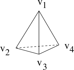
Proof. This boils down to the followoing calculation, illustrated on Figure 15: \[\begin{align} &\frac{\omega(v_2, v_3)}{\omega(v_1, v_2)\omega(v_1, v_3)} + \frac{\omega(v_3, v_4)}{\omega(v_1, v_3)\omega(v_1, v_4)} = \\ &\frac{ \omega(v_2,v_3)\omega(v_1,v_4)+ \omega(v_1, v_2)\omega(v_3, v_4)}{\omega(v_1, v_2)\omega(v_1, v_3)\omega(v_1, v_4)} \stackrel{}{=}\\ &\frac{ \omega(v_1,v_3)\omega(v_2,v_4)}{\omega(v_1, v_2)\omega(v_1, v_3)\omega(v_1, v_4)} = \frac{ \omega(v_2,v_4)}{\omega(v_1, v_2)\omega(v_1, v_4)}.\\ \end{align}\] Here the second equality is the provided by the Plücker relation. ◻
Denote by \(W^\delta_{{\Bbb S}'}\) the potential on \({\cal P}_{{\Bbb S}'}^\delta\). Lemma 8 implies that \[\label{-1eq} {W_{\Bbb S}} = {\rm cut}^*_{\rm E}(W^\delta_{{\Bbb S}'}).\tag{52}\]
::: {#PROP2.9+ .proposition} Proposition 16. One has \[\begin{align} & e^{-W_{\Bbb S}}\Omega_{\Bbb S}({\rm K}) = {\rm cut}^*_{\rm E} \Bigl(e^{-W^\delta_{{\Bbb S}'}}\Omega^\delta_{{\Bbb S}'}({\rm K}_{\rm E},{\rm K}) \Bigr)\wedge d\log {\rm K}_{\rm E} . \end{align}\] :::
Proof. Follows from (?? ) and (52 ). ◻
2.2.5 Cutting along a simple closed geodesic.↩︎
For the punctured disc with \(n\) marked boundary points \({\rm D}_n^*\), the dimension of moduli space \({\cal P}_{{\rm D}_n^*}\) is \(2n\). There is canonical ideal triangulation shown on Figure 18. Let \({\rm K}_1,...,{\rm K}_n\) and \({\rm B}_1,...,{\rm B}_n\) be the \({\rm K}\)- and \({\rm B}\)-variables at the boundary intervals, and \({\rm X}_1,...,{\rm X}_n\) the variables at the internal edges of the triangulation. Then \(\{{\rm X}_1,...,{\rm X}_n,{\rm B}_1,...,{\rm B}_n\}\) are the cluster Poisson coordinates on the moduli space \({\cal P}_{{\rm D}_n^*}\) [12]. Let \({\rm L}_1=e^{l_1}\) be the product of the cluster Poisson coordinates at the edges sharing the puncture. Let the \({\rm E}\)-parameters be \[{\rm E}:= {\rm K}_1 \cdots {\rm K}_{n}.\] By [12], the functions \({\rm E}\) and \({\rm L}_1\) are algebraically independent and generate the center of the Poisson algebra \({\cal O}({\cal P}_{{\rm D}_n^*})\). We call them the Casimirs. Thus the cluster Poisson structure induces a symplectic \(2\)-form \(\omega_{\rm cl}\) on the fiber \({\cal P}_{{\rm D}_n^*}({\rm E},{\rm L}_1)\) where \({\rm E}\) and \({\rm L}_1\) are fixed.
For a genus \(g\) ideal hyperbolic surface \({\Bbb S}\) with ideal crowns \({\rm C}_1,\ldots, {\rm C}_r\) with \((n_i)_{i=1}^r\) cusps and \(m-r\) boundary geodesic circles, the dimension of moduli space \({\cal P}_{{\Bbb S}}\) is \(6g-6+3m+2\sum_{i=1}^r n_i\). We denote the \({\rm E}\)-parameters of \({\rm C}_1,\ldots, {\rm C}_r\) by \({\rm E}=({\rm E}_1,\ldots,{\rm E}_{r})\). Let \({\rm L}=(l_{r+1},\ldots, l_m)\) be the geodesic lengths of the boundary geodesic circles, and \(({\rm L}_{r+1}, ..., {\rm L}_{m})\) their exponents. By [12], the functions \({\rm E}_1,...,{\rm E}_r\) and \({\rm L}_{r+1},...,{\rm L}_m\) are algebraically independent Casimirs, generating the center of the Poisson algebra \({\cal O}({\cal P}_{{\Bbb S}})\). Thus the cluster Poisson structure on \({\cal P}_{{\Bbb S}}\) induces a symplectic \(2\)-form \(\omega_{\rm cl}\) on \({\cal P}_{{\Bbb S}}({\rm E},{\rm L})\).
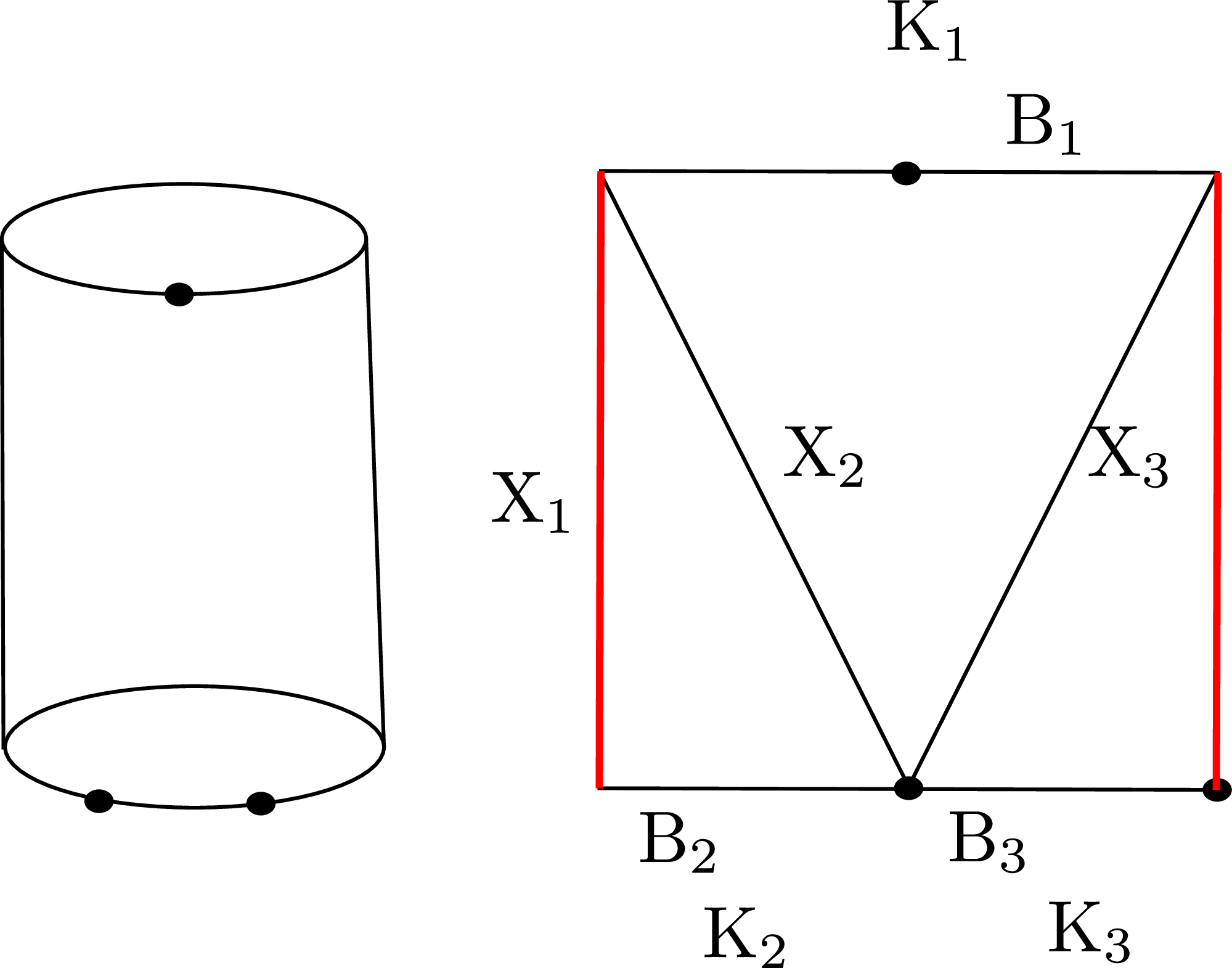
Here is an example. The cluster Poisson coordinates on moduli space \(\mathcal{P}_{{\rm A}_{1,2}}\) for the annulus \({\rm A}_{1,2}\) with \(2+1\) boundary points, for the triangulation on Figure 16, are \({\rm X}_1\), \({\rm X}_2\), \({\rm X}_3\), \({\rm B}_1\), \({\rm B}_2\), \({\rm B}_3\). The \({\rm K}-\)coordinates are monomials in the cluster Poisson coordinates: \[{\rm K}_1= {\rm B}_1^2 {\rm X}_1 {\rm X}_2 {\rm X}_3,\;\;\; {\rm K}_2= {\rm B}_3 {\rm X}_3 {\rm X}_2 {\rm B}_2,\;\;\; {\rm K}_3= {\rm B}_2 {\rm X}_1 {\rm B}_3.\] The \({\rm K}_1\) and \({\rm K}_2 {\rm K}_3\) are the Casimirs.
For a simple closed geodesic \(\gamma\), let \({\Bbb S}'\) be the decorated surface obtained by cutting \({\Bbb S}\) along \(\gamma\), which has two new simple closed geodesics \(\gamma'\), \(\gamma''\) corresponding to the original \(\gamma\). We define a rational map \({\cal P}_{{\Bbb S}} \longrightarrow{\cal P}_{{\Bbb S}'}\) by restricting a local system on \({\Bbb S}\) to \({\Bbb S}'\), and inducing the decorations and framing. Its image lies in the subspace \({\cal P}^\delta_{{\Bbb S}'}\), defined by the equation \(l_\gamma=l_{\gamma'}\not = 0\). We arrive at the rational cutting map \[\label{cut3} {\rm cut}_\gamma: {\cal P}_{{\Bbb S}} \longrightarrow{\cal P}^\delta_{{\Bbb S}'}.\tag{53}\]
Proposition 17. There is a positive constant \(c_{{\Bbb S},\gamma}\) depending only on \({\Bbb S}\) and \(\gamma\) such that \[\Omega_{\Bbb S}({\rm E},{\rm L}) = c_{{\Bbb S},\gamma} \cdot{\rm cut}^*_{\gamma} \Bigl(\Omega^\delta_{{\Bbb S}'}({\rm E},{\rm L},{\rm L}_\gamma) \Bigr)\wedge d \l_\gamma \wedge d \theta_\gamma,\] restricts to \[\Omega_{\Bbb S}({\rm K},{\rm L}) = c_{{\Bbb S},\gamma} \cdot{\rm cut}^*_{\gamma} \Bigl(\Omega^\delta_{{\Bbb S}'}({\rm K},{\rm L},{\rm L}_\gamma) \Bigr)\wedge d \l_\gamma \wedge d \theta_\gamma.\]
Remark 18. We conjecture that \(c_{{\Bbb S},\gamma}=2^{ \pi_0({\Bbb S})-\pi_0({\Bbb S}-\gamma)}\). We checked that it holds for any surface with punctures but without marked boundary points. The \(n\)-holed sphere case is proved in Appendix 10.
Proof. To follow the notation in [20], we will use the lambda lengths parameters, expressed via our \({\rm K}-\)coordinates by \(\lambda_x={\rm K}_x^{-\frac{1}{2}}\). Then, as in Figure 17, we have \[{\rm B}_a=\frac{\lambda_b}{\lambda_a \lambda_e},\;\;\; {\rm B}_b=\frac{\lambda_e}{\lambda_a \lambda_b},\;\;\; {\rm X}_e=\frac{\lambda_a \lambda_c}{\lambda_b \lambda_d},\;\;\; {\rm X}_d=\frac{\lambda_e \lambda_f}{\lambda_c \lambda_g}.\]
The Goldman bracket between two geodesic/\(\lambda\)-lengths \(\{\cdot,\cdot\}\) is given in [20]. When two arcs \(x, y\) intersect at a boundary cusp \(p\) and the arc \(x\) orients clockwise towards the arc \(y\) we have \[\label{bclam} \{\lambda_x,\lambda_y\}=\frac{1}{4}\lambda_x \cdot \lambda_y,\tag{54}\]
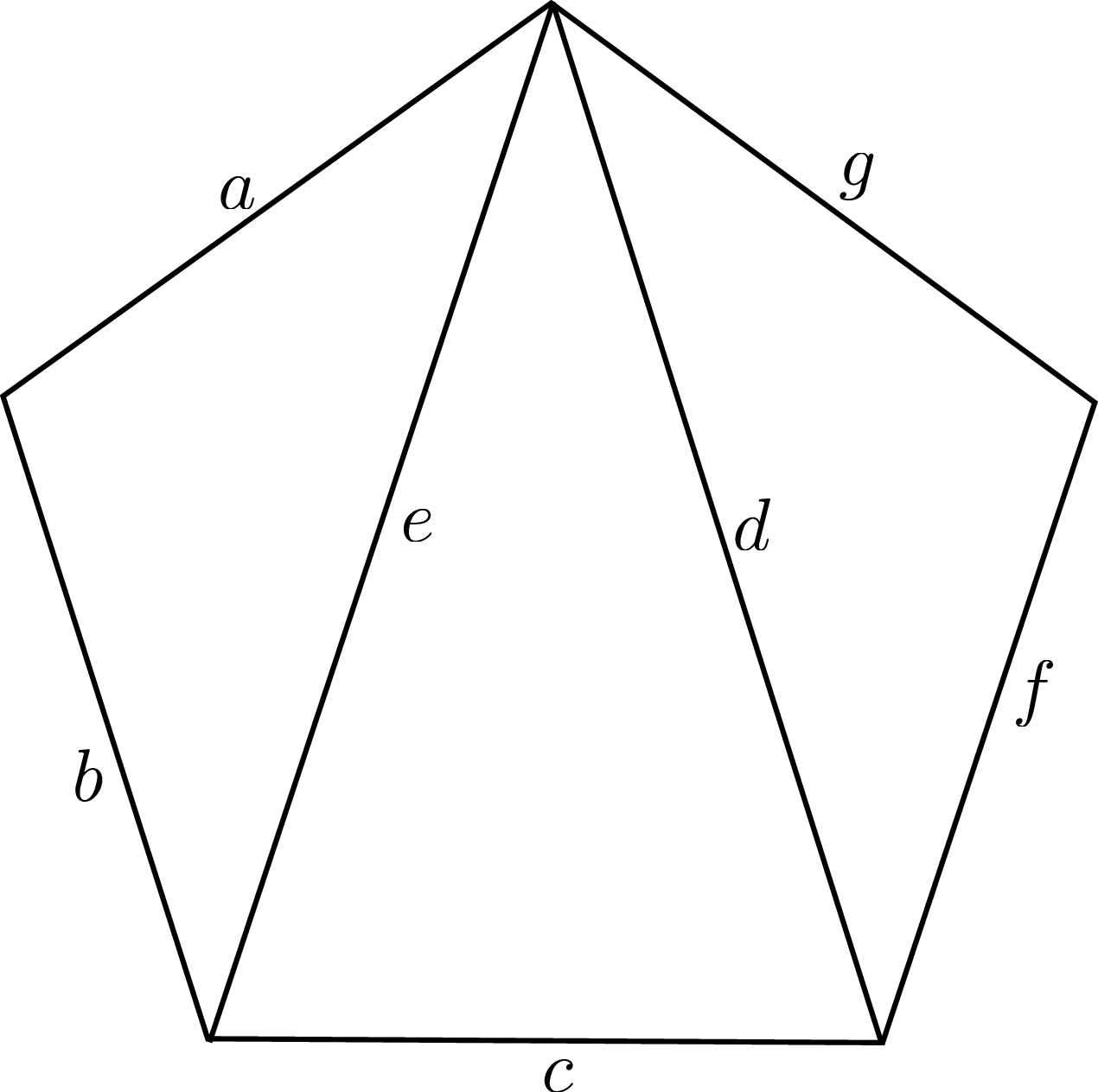
Then by formula 54 we obtain
\[\{{\rm B}_a,{\rm B}_b\}={\rm B}_a {\rm B}_b, \;\;\; \{{\rm B}_b,{\rm X}_e\}={\rm B}_b {\rm X}_e,\;\;\; \{{\rm X}_d,{\rm X}_e\}={\rm X}_d {\rm X}_e.\] So cluster Poisson structure on \({\cal T}_{{\Bbb S}}\subset {\cal T}^{\rm en}_{{\Bbb S}}={\cal P}_{{\Bbb S}}(\mathbb{R}_{>0})\) coincides with the Goldman Poisson structure defined by curves and their intersections.
The neck geodesic circles \(\gamma_1,...,\gamma_r\) cut \({\Bbb S}\) into \(S_{g,m}\cup {\rm C}_1\cup ...\cup {\rm C}_r\). Let \(l_1,...,l_r, \theta_1,...,\theta_r\) be the length and twist parameters of \(\gamma_1,...,\gamma_r\) and set \({\rm L}_i=e^{l_i}\). Then \({\cal T}_{{\Bbb S}}\) is parametrised by the following parameters:
\(l_1,...,l_r, \theta_1,...,\theta_r\),
the parameters \(l_{\alpha_1},..., l_{\alpha_{3g-3+m}}\), \(\theta_{\alpha_1},..., \theta_{\alpha_{3g-3+m}}\) for \({\cal T}_{S_{g,m}}({\rm L}_1,...,{\rm L}_r)\) with the pants decomposition \(\{\alpha_{1},...,\alpha_{3g-3+m}\}\),
the parameters for the spaces \({\cal T}_{{\rm C}_1}({\rm L}_1)\), \(...\), \({\cal T}_{{\rm C}_r}({\rm L}_r)\).
By [20], for any \(i=1,...,r\), the twist function \(\theta_i\) can be written explicitly as a function of curves near \(\gamma_i\). Then by [20], we have \[\{l_i,\theta_i\}=1,\;\;\; \{u, \theta_i\}=0, \;\;\;\{l_i, u\}=0,\] for any parameter \(u\) of \({\cal T}_{S_{g,m}}({\rm L}_1,...,{\rm L}_r)\) or any \(u\) of \(l_1,..., \widehat l_{i},...,l_r\), \(\theta_1,...,\widehat \theta_{i},...,\theta_r\). When \(\gamma_i\) is not the neck geodesic of the crown \({\rm C}_j\), by adding decoration at \(\gamma_i^+\), we express any cluster coordinate \(u\) of \({\cal T}_{{\rm C}_j}({\rm L}_j)\) as a ratio of products of \(\lambda-\)lengths of arcs in \({\rm C}_j\). Since the curve \(\gamma_i\) does not intersect with the arcs for \(u\), \[\{u, \theta_i\}=0, \;\;\;\{l_i, u\}=0.\] When \(\gamma_i\) is the neck geodesic of the crown \({\rm C}_j\), the ideal arc \(\ell_0\) starting and ending at a cusp \(p\) cuts \({\rm C}_j\) into \({\rm D}_{n_j+1}\cup {\rm D}_1^*\). The parameter \({\rm K}_0\) is the \({\rm K}\)-parameter along \(\ell_0\). Then \({\cal T}_{{\rm C}_j}({\rm L}_j)\) is parametrised by \({\rm K}_0,{\rm K}_1,...,{\rm K}_{n_j}\), \({\rm X}_1,...,{\rm X}_{n_j-2}\) for an ideal triangulation of \({\rm D}_{n_j+1}\). The length function \(l_i\) is a Casimir on \({\cal T}_{{\rm C}_j}\) for the cluster Poisson structure. The term of twist function \(\theta_i\) in [20] intersecting with \({\rm C}_j\) is \({\rm X}_{A^k B}:=\frac{\lambda_{A^k B}}{\lambda_{0}}\), where \(A^k B\) is some curve starting and ending at \(p\), surrounding some loop as in [20], and \(\lambda_{0}={\rm K}_0^{-\frac{1}{2}}\). Both \(A^k B\) and \(\ell_0\) intersect with \({\rm D}_{n_j+1}\) at \(p\), thus \(\{{\rm X}_{A^k B}, u\}=0\) for any paramter \(u\) of \({\cal T}_{{\rm C}_j}({\rm L}_j)\). So \(\{\theta_i, u\}=0\) for any paramter \(u\) of \({\cal T}_{{\rm C}_j}({\rm L}_j)\)...... Hence we can write twice the cluster symplectic form \(2\omega_{\rm cl}\) on \({\cal T}_{{\Bbb S}}({\rm E},{\rm L})\) as:9 \[\label{eq:wcut} 2\omega_{\rm cl}=\sum_{i=1}^{r}d l_i \wedge d \theta_i+\omega_{\rm gm}+\sum_{i=1}^r \omega_{i},\tag{55}\] where \(\omega_{\rm gm}=\sum_{i=1}^{3g-3+m} d l_{\alpha_i} \wedge d \theta_{\alpha_i}\) is the Weil–Petersson form on \({\cal T}_{S_{g,m}}({\rm L}_1,...,{\rm L}_r,{\rm L})\) for the pants curves \(\alpha_i\), and \(\omega_{i}\) is twice the cluster symplectic form on \({\cal T}_{{\rm C}_i}({\rm E}_i,{\rm L}_i)\), which has a normalized expression in Darboux coordinates. The above description of the cluster/Goldman Poisson structure naturally extends from \({\cal T}_{{\Bbb S}}\) to \({\cal P}_{{\Bbb S}}\). Thus we define the Weil–Petersson volume form on \({\cal P}_{{\Bbb S}}({\rm E},{\rm L})\) to be \[\Omega^{\rm WP}_{\Bbb S}({\rm E},{\rm L}):=\frac{(2\omega_{\rm cl})^d}{d!}, \;\;\;\;\;\;d:= \frac{1}{2}{\rm dim}{\cal P}_{{\Bbb S}}({\rm E},{\rm L}).\]
Suppose \(\gamma\) is one of the pants curves \(\alpha_j\). Then by direct computation, we get \[\label{vel0} \Omega^{\rm WP}_{\Bbb S}({\rm E},{\rm L})=\Omega^{\rm WP}_{{\Bbb S}'}({\rm E},{\rm L}') \wedge d l_\gamma \wedge d \theta_\gamma,\tag{56}\] where \({\rm L}'=({\rm L},l_{\gamma'},l_{\gamma''})\). Now let us relate the Weil–Petersson volume form \(\Omega^{\rm WP}_{\Bbb S}({\rm E},{\rm L})\) to the cluster volume form \(\Omega_{\Bbb S}({\rm E},{\rm L})\). Given an ideal triangulation \(\mathcal{T}\) of the decorated surface \({\Bbb S}\), we have the cluster Poisson structure on \({\cal P}_{{\Bbb S}}\) induced by the cluster quiver \(\epsilon_{ij}\) on \({\Bbb S}\) with respect to the orientation of \({\Bbb S}\). The cluster volume form is \(\Omega_{\Bbb S}=2^{\pi_0({\Bbb S})} \bigwedge_i d x_i\) where \(x_i\) is the log of the cluster variable \({\rm X}_i\). Then we choose \(2d\) variables \(\{y_i\}_{i=1}^{2d}\) among them such that the determinant \(\det_{\Bbb S}\) of sub matrix of the skew-symmetric matrix for the quiver is non-zero. Thus we have \[\label{vel1} \frac{\bigwedge_{i=1}^{2d} d y_i}{\sqrt{\det_{\Bbb S}}}= \frac{\omega_{\rm cl}^d}{d!}.\tag{57}\] On the other hand, by \[\Omega_{\Bbb S}({\rm E},{\rm L}) \wedge \bigwedge_{i=1}^{r} d \log {\rm E}_i \wedge \bigwedge_{i=r+1}^{m} d l_i=2^{\pi_0({\Bbb S})}\bigwedge_i d x_i.\] we get \[\label{vel2} \bigwedge_{i=1}^{2d} d y_i=d_{\Bbb S}\Omega_{\Bbb S}({\rm E},{\rm L}),\tag{58}\] for some positive rational constant \(d_{\Bbb S}\). Combining with equations (57 )(58 ), we obtain \[\label{vel3} \frac{2^d d_{\Bbb S}}{\sqrt{\det_{\Bbb S}}}\Omega_{\Bbb S}({\rm E},{\rm L})= \frac{\omega_{\rm WP}^d}{d!}.\tag{59}\] Since \(\frac{\omega_{\rm WP}^d}{d!}\) and \(\Omega_{\Bbb S}({\rm E},{\rm L})\) are invariant under the cluster transformations, the number \(\frac{2^d d_{\Bbb S}}{\sqrt{\det_{\Bbb S}}}\) is also invariant under the cluster transformations, hence a constant depending only on \({\Bbb S}\). Plugging equation (59 ) into equation (56 ), we get \[\Omega_{\Bbb S}({\rm E},{\rm L}) = c_{{\Bbb S},\gamma} \cdot{\rm cut}^*_{\gamma} \Bigl(\Omega^\delta_{{\Bbb S}'}({\rm E},{\rm L},{\rm L}_\gamma) \Bigr)\wedge d \l_\gamma \wedge d \theta_\gamma,\] where \(c_{{\Bbb S},\gamma}=\frac{2 d_{\Bbb S}\sqrt{\det_{{\Bbb S}'}}}{d_{{\Bbb S}'} \sqrt{\det_{{\Bbb S}}}}\) depending only on \({\Bbb S}\) and \(\gamma\). ◻
Proof of Theorem 2. By applying Proposition 17 to the neck geodesics, combining with [13], we obtain Theorem 2. ◻
3 The exponential volumes of moduli spaces and \({\cal B}-\)functions↩︎
3.1 \({\cal B}-\)functions of decorated surfaces↩︎
Recall the parameters \({\rm K}\) in (2 ), and the \({\cal B}-\)function from Section 1.2: \[\label{EIa} \begin{align} {\mathcal{B}}_{\Bbb S}({{\rm K}}, s_1, ..., s_m; \hbar) :=&\int_{{\cal M}^{\circ \circ}_{\Bbb S}}e^{-W/\hbar} \; e^{-(l_1 s_1 + ... +l_m s_m)/2} \;\Omega_{\Bbb S}({{\rm K}}).\\ \end{align}\tag{60}\]
3.1.0.1 Example 1.
Let \({\Bbb S}= {\rm D}^*_n\) be the punctured disc with \(n\) marked points \(x_1, ..., x_n\), see Figure 18. It has an ideal triangulation given by the internal edges \({\rm E}_1, ..., {\rm E}_n\) connecting the puncture with the points \(x_1, ..., x_n\), and the boundary edges \({\rm F}_i = x_{i-1}x_{i}\). The pure mapping class group is trivial. So the Teichmüller and the moduli spaces are the same. They parametrise ideal hyperbolic structures on the crown with a choice of the eigenvalue of the monodormy around the boundary loop. Denote by \({\rm X}_i\) and \({\rm B}_i\) the cluster Poisson coordinates assigned to the edges \({\rm E}_i\) and \({\rm F}_i\). Then the cluster volume form is \[\Omega_{{\cal P}_{{\rm D}_n^*}}= 2 d\log {\rm X}_1 \wedge \ldots \wedge d\log {\rm X}_n \wedge d\log {\rm B}_1\wedge \ldots \wedge d\log {\rm B}_n.\] The \({\rm K}-\)variable along \(x_{i-1} x_{i}\), see Figure 18, is calculated by: \[\label{KXBB} {\rm K}_{i+1} = {\rm B}_{i}{\rm X}_{i}{\rm B}_{i+1}, \quad i \in {\mathbb{Z}}/n{\mathbb{Z}}.\tag{61}\]
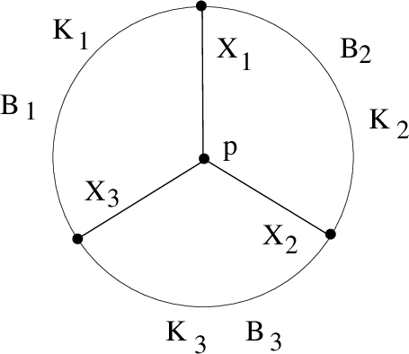
Then \[{\rm X}_i = {\rm K}_{i+1}/({\rm B}_i{\rm B}_{i+1}).\] The potential at the cusp \(x_i\) is given by \[W_i:= {\rm B}_i + {\rm B}_i{\rm X}_i = {\rm B}_i + \frac{{\rm K}_{i+1}}{{\rm B}_{i+1}}.\] Therefore the total potential is given in the coordinates \(\{{\rm B}_i, {\rm K}_i\}\) by \[W:= \sum_{i\in {\mathbb{Z}}/n{\mathbb{Z}}}W_i= \sum_{i\in {\mathbb{Z}}/n{\mathbb{Z}}} \left({\rm B}_i + \frac{{\rm K}_i}{{\rm B}_{i}}\right).\] We set \[\label{MNOaa} \begin{align} &{\boldsymbol{B}}:= {\rm B}_1 \cdot \cdot \cdot {\rm B}_n, \qquad {\boldsymbol{K}}:= {\rm K}_1 \cdot\cdot\cdot {\rm K}_n. \\ \end{align}\tag{62}\] The square \({\rm L}\) of the largest eigenvalue of the monodromy around the boundary loop is calculated from the following formulas: \[\label{LX} {\rm L}:= e^l = {\rm X}_1\cdots {\rm X}_n={\boldsymbol{K}}/{\boldsymbol{B}}^2.\tag{63}\] So the geodesic length \(l\) of the neck geodesic \(\ell\) is \(l = \log ({\rm X}_1 \cdots {\rm X}_n)\).
We consider the variables \({\rm K}= ({\rm K}_1, \ldots {\rm K}_n)\) as fixed parameters. Then the fiberwise volume form is \[\Omega_{\Bbb S}({\rm K}) :=2d\log {\rm B}_1 \wedge \ldots \wedge d\log {\rm B}_{n}.\] Indeed, it satisfies the following relation, where according to (61 ), we have \({\rm K}_{i +1}= {\rm X}_i{\rm B}_i{\rm B}_{i+1}\): \[d\log {\rm K}_1 \wedge \ldots \wedge d\log {\rm K}_n \wedge \Omega_{\Bbb S}({\rm K}) = 2 d\log {\rm X}_1 \wedge \ldots \wedge d\log {\rm X}_n \wedge d\log {\rm B}_1\wedge \ldots \wedge d\log {\rm B}_n.\]
Recall the Bessel function: \[\label{f22*} \begin{align} J_s(z):=&\int_{0}^\infty {\rm exp}\Bigl({-\sqrt{z}(\lambda+\lambda^{-1}} )\Bigr)\lambda^{s} d\log {\lambda} \;= \;z^{-s/2}\cdot \int_{0}^\infty {\rm exp}\Bigl({-t-\frac{z}{t}} \Bigr)t^{s} d\log {t}.\\ \end{align}\tag{64}\]
3.1.0.2 1.
For the decorated surface \({\rm D}_1^*\) the cluster Poisson coordinates are \({\rm B}, {\rm X}\). So \({\rm L}= e^l = {\rm X}={\rm K}/{\rm B}^2,\) and10 \[\label{89} \begin{align} {\cal B}_{{\rm D}^*_1}({\rm K}, s) =\;&\int_{0}^\infty e^{-({\rm B}+\frac{{\rm K}}{{\rm B}})} {\rm L}^{-s/2} \cdot 2d \log {\rm B}= 2 \int_{0}^{\infty} e^{-({\rm B}+\frac{{\rm K}}{{\rm B}})} \left(\frac{{\rm K}}{{\rm B}^2}\right)^{-s/2} d\log {\rm B} =\; 2 J_{s}({\rm K}). \\ \end{align}\tag{65}\] This recovers formula (14 ).
3.1.0.3 2.
Let \({\Bbb S}={\rm D}_n^*\). We set \({\Bbb K}:=\{{\rm K}_1, \ldots {\rm K}_n\}\), and introduce the notation \[\label{MNOa} \begin{align} & J_{s}({{\Bbb K}}):= J_{s}({\rm K}_1) \cdot \cdot \cdot J_{s}({\rm K}_n). \\ \end{align}\tag{66}\] Then we have, using (63 ): \[\label{56} \begin{align} {\cal B}_{{\rm D}_{n}^*}({{\rm K}}, s) = \;&\int e^{-W} {\rm L}^{-s/2}\Omega_{{\rm D}_n^*} \\ = \;& \int_{{\rm B}_i>0} e^{-({\rm B}_1+\frac{K_1}{{\rm B}_1} +\ldots + {\rm B}_n + \frac{K_n}{{\rm B}_n}) } \left( \frac{{\boldsymbol{K}}}{{\boldsymbol{B}}^2}\right)^{-s/2} \cdot 2 d\log {\rm B}_1 \wedge \ldots \wedge d\log {\rm B}_{n} \\ = \;& 2 J_{s}({{\rm K}_1})\cdots J_{s}({{\rm K}_n}) \stackrel{(\ref{MNOa})}{=}:\;2 J_{s}({\Bbb K}).\\ \end{align}\tag{67}\]
Recall that \(r\) is the number of crown ends of a decorated surface \({\Bbb S}\), so that \(m-r\) is the number of punctures on \({\Bbb S}\). We denote by \(J_{s_i}({\Bbb K}_i)\) the function (66 ) for the \(i-\)th crown, where \(1 \leq i \leq r\). Recall \({\rm C}_{{\Bbb S}, \ell}:=2^{-\mu_\ell} c_{{\Bbb S}, \ell}\) where \(\mu_\ell\) is the number of one-holed tori cutting off by \(\ell\) and \(c_{{\Bbb S}, \ell}\) is a positive constant depending only on \({\Bbb S}\) and \(\ell\) defined in Proposition 17.
Theorem 19. The integral \({\cal B}_{{\Bbb S}}({{\rm K}}, s_1, ... , s_m)\) is finite if \({\rm Re}(s_i>0)\), and can be analytically continued and calculated as follows, where \(|k|=k_1+...+k_m\): \[\label{MFOEa} \begin{align} &{\cal B}_{{\Bbb S}}({{\rm K}}, s_1, ... , s_m) \;= {\rm C}_{\Bbb S}\sum_{k_1+ ... + k_m\leq 3g-3+m} {\cal V}_{g, k_1, ..., k_m} 2^{m} \; \prod_{i=1}^r-\Bigl(2\frac{d}{ds_i}\Bigr)^{2k_i+1} J_{s_i}({\Bbb K}_i)\cdot \prod_{j=r+1}^m \frac{(2k_j)!}{s_j^{2k_j+1}}. \\ \end{align}\qquad{(18)}\]
Proof. By Mirzakhani’s theorem (6 ) the volume of the moduli space \(\mathcal{M}_S({\rm L})\) of the genus \(g\) surfaces \(S\) with boundary geodesics of the lengths \(l_1, ..., l_m\) is given by: \[\label{V1*} {\rm Vol}(\mathcal{M}_S({\rm L})) = \sum_{k_1, ..., k_m \leq 3g-3+m} {\cal V}_{g, k_1, ..., k_m}l_1^{2k_1} \cdots l_m^{2k_m}.\tag{68}\] Therefore the enhanced variant of the neck recursion formula ?? implies the following formula: \[\label{MFOE} \begin{align} {\cal B}_{{\Bbb S}}({{\rm K}}, s_1, ..., s_m) = {\rm C}_{\Bbb S}\sum_{k_1+ ... + k_m\leq 3g-3+m} {\cal V}_{g, k_1, ..., k_m} \cdot &\\ \prod_{i=1}^r \int_{-\infty}^{\infty} { \rm Vol}_{\mathcal{E}}({\rm D}_{n_i}^*)({{\rm K}}_i,l_i) \;e^{-l_is_i/2} \;l_i^{2k_i+1} d l_i\cdot & \prod_{j=r+1}^m \int_0^\infty e^{-l_js_j/2} \;l_j^{2k_j}dl_j. \\ \end{align}\tag{69}\] Using formula (67 ), the integral for the punctured disc \({\rm D}_n^*\) appearing in (69 ) is calculated as follows: \[\begin{align} & \int e^{-W_{}} e^{-ls/2} \;l^{2k+1} \Omega_{{\rm D}_n^*} = 2 \Bigl(-2\frac{d}{ds}\Bigr)^{2k+1} J_{s}({\Bbb K}). \\ \end{align}\] Theorem 19 is proved. ◻
A similar approach to the function \({\cal L}_{\Bbb S}({\rm K}; s)\) does not lead to a formula expressing it via Bessel functions.
3.1.0.4 Example 2.
For a once crowned torus \({\Bbb S}\) with \(n\) cusps on Figure 19, we have \[\begin{align} {\cal B}_{{\Bbb S}}({{\rm K}}, s)\;= \; & \frac{1}{2} \left(\frac{\pi^2}{6}\int_{-\infty}^{+\infty} { \rm{Vol}}_{\mathcal{E}}({\cal M}_{{\rm D}_{n}^*})({{\rm K}},l)\;e^{-ls/2} \;l \;d l+\frac{1}{24}\int_{-\infty}^{+\infty} {\rm{Vol}}_{\mathcal{E}}({\cal M}_{{\rm D}_{n}^*})({{\rm K}},l)\;e^{-ls/2} \;l^3 \;d l\right)\\ =\;& -\frac{1}{3}\Bigl(\pi^2 \frac{d}{ds}+ \frac{d^3}{ds^3}\Bigr)J_{s}({{\rm K}}). \\ \end{align}\]
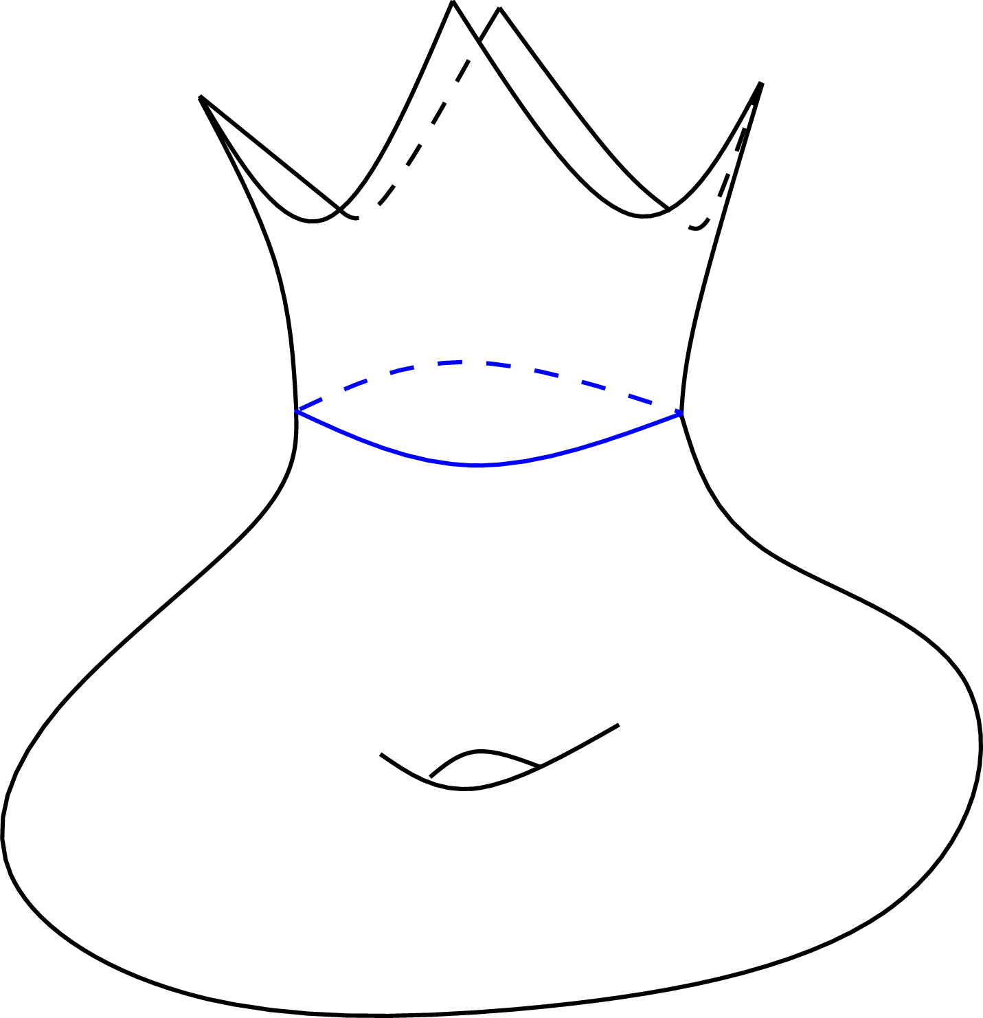
Indeed, the Weil–Petersson volume of the moduli space \({\cal M}_{1,1}(l)\) of hyperbolic structures on a torus with a single hole of the geodesic length \(l\) is given by [13] by the formula \[{\rm Vol}({\cal M}_{1,1}(l) )= \frac{\pi^2}{6} + \frac{l^2}{24}.\]
3.2 The exponential volume of the crown↩︎
Recall the Bessel function \[\begin{align} J_0(z)= \int_{0}^\infty {\rm exp}\Bigl({-t-\frac{z}{t}} \Bigr) d\log {t}.\\ \end{align}\] We use below both notations \({\rm D}_n^*({{\rm K}}; {\rm L}) = {\rm D}_n^*({{\rm K}}; l)\), where \({\rm L}\) and \(l\) are related by \({\rm L}=e^l\).
To get the volume \({\rm Vol}_{\mathcal{E}}({\rm D}_n^*)({{\rm K}}; {\rm L})\), we integrate the form over the positive locus \(B_i \geq 0\) the form \[\Omega_{\rm B}':= 2 d\log {\rm B}_1 \wedge \ldots \wedge d\log {\rm B}_{n-1}.\]
Lemma 9. For \(n=2\), we get \[\label{FLe4.1} {\rm{Vol}}_{\mathcal{E}}({\rm D}_2^*)({\rm K}_1, {\rm K}_2; {\rm L}) = J_0({\rm K}_1+{\rm K}_2+\sqrt{{\rm K}_1 {\rm K}_2}({\rm L}^{1/2}+ {\rm L}^{-1/2})).\qquad{(19)}\]
Proof. Since \({\rm X}_1={\rm K}_2/({\rm B}_1 {\rm B}_2)\) and \({\rm X}_2={\rm K}_1/({\rm B}_1 {\rm B}_2)\), we obtain \({\rm B}_1 {\rm B}_2=e^{-l/2}\sqrt{{\rm K}_1 {\rm K}_2}\). So the integral is \[\begin{align} &\int_{0}^\infty{\rm exp}\Bigl(-{\rm B}_1-{\rm K}_1/{\rm B}_1-e^{-l/2}\sqrt{{\rm K}_1 {\rm K}_2}/{\rm B}_1- {\rm B}_1e^{l/2} {\rm K}_2/\sqrt{{\rm K}_1 {\rm K}_2}\Bigr) d \log {\rm B}_1 \\ &= J_0({\rm K}_1+{\rm K}_2+\sqrt{{\rm K}_1 {\rm K}_2 }(e^{l/2}+e^{-l/2})). \end{align}\] ◻
Lemma 10. The integral \(\rm{Vol}_{\mathcal{E}}({\rm D}_n^*)({{\rm K}}; {\rm L})\) is finite.
Proof. Since \({\rm B}_n + \frac{{\rm K}_{n}}{{\rm B}_{n}}> 0\), we obtain \[\begin{align} &{\rm Vol}_{\mathcal{E}}({\rm D}_n^*)({{\rm K}}; {\rm L})=\int_{{\rm B}_1 > 0}\cdots\int_{{\rm B}_{n-1} > 0}{\rm exp}\Bigl(-\sum_{i=1}^n \Bigl({\rm B}_i + \frac{{\rm K}_{i}}{{\rm B}_{i}}\Bigr)\Bigr) \Omega'_{\rm B}\\ &< 2 \prod_{i=1}^{n-1}\int_0^\infty {\rm exp}\Bigl(-{\rm B}_i - \frac{{\rm K}_{i}}{{\rm B}_{i}}\Bigr)d\log {\rm B}_i = 2\prod_{i=1}^{n-1}J_0({\rm K}_i). \end{align}\] ◻
It seems hard to obtain an explicit formula for \(n\geq 3\).
Proposition 20. For any integer \(k\geq 0\), the integral \(\int_{0}^{+\infty} {\rm Vol}_{\mathcal{E}}({\rm D}_n^*)({{\rm K}},l)l^k d l\) is finite.
Proof. Since \({\rm B}_1 \cdots {\rm B}_n=e^{-l/2}\sqrt{{\rm K}_1\cdots {\rm K}_n}\), we get \[\label{120} \begin{align} &\int_{0}^{+\infty} {\rm Vol}_{\mathcal{E}}({\rm D}_n^*)({{\rm K}},l)l^k d l =\\ &\int_{0}^{+\infty} \int_{{\rm B}_1 > 0}\cdots\int_{{\rm B}_{n-1} > 0}{\rm exp}\Bigl(-\sum_{i=1}^n \Bigl({\rm B}_i + \frac{{\rm K}_{i}}{{\rm B}_{i}}\Bigr)\Bigr) \Omega'_{\rm B}\cdot l^k d l =\\ &\int_{{\rm B}_1 > 0}\cdots\int_{{\rm B}_{n-1} > 0}{\rm exp}\Bigl(-\sum_{i=1}^{n-1} \Bigl({\rm B}_i + \frac{{\rm K}_{i}}{{\rm B}_{i}}\Bigr)\Bigr) \int_{0}^{+\infty} {\rm exp}\Bigl(-\frac{{\rm K}_1^{1/2}\cdots {\rm K}_n^{1/2}}{{\rm B}_1 \cdots {\rm B}_{n-1}}e^{-l/2}-\frac{{\rm B}_1 \cdots {\rm B}_{n-1}{\rm K}_n}{{\rm K}_1^{1/2}\cdots {\rm K}_n^{1/2}}e^{l/2}\Bigr) l^k d l \cdot \Omega'_{\rm B}. \end{align}\tag{70}\] Note that we have \[\begin{align} &\int_{0}^{+\infty} {\rm exp}\Bigl(-\frac{{\rm K}_1^{1/2}\cdots {\rm K}_n^{1/2}}{{\rm B}_1 \cdots {\rm B}_{n-1}}e^{-l/2}-\frac{{\rm B}_1 \cdots {\rm B}_{n-1}{\rm K}_n}{{\rm K}_1^{1/2}\cdots {\rm K}_n^{1/2}}e^{l/2}\Bigr) l^k d l \\ &\leq \frac{1}{k+1}\int_{0}^{+\infty} {\rm exp}\Bigl(-\frac{{\rm B}_1 \cdots {\rm B}_{n-1}{\rm K}_n}{{\rm K}_1^{1/2}\cdots {\rm K}_n^{1/2}}\frac{l^{k+1}}{2^{k+1}(k+1)!}\Bigr) d l^{k+1}\leq {}\frac{\rm C}{{\rm B}_1 \cdots {\rm B}_{n-1}}. \end{align}\] Here \({\rm C}\) is a constant. Therefore \[\begin{align} &\int_{0}^{+\infty}{ \rm Vol}_{\mathcal{E}}({\rm D}_n^*)({{\rm K}},l)l^k d l \leq 2 {\rm C}\cdot \prod_{i=1}^{n-1} \int_{{\rm B}_i > 0} {\rm exp}\Bigl(- \Bigl({\rm B}_i + \frac{{\rm K}_{i}}{{\rm B}_{i}}\Bigr)\Bigr) {\rm B}_i^{-2} d {\rm B}_i \end{align}\] which converges. ◻
3.3 The general exponential volumes↩︎
Consider the genus \(g\) decorated surface \({\Bbb S}\) with \(m\) boundary components. Denote by \(n_1, ..., n_r\) the numbers of cusps on the crowns. Recall notation (2 ) for \({{\rm K}} = \{{{\rm K}}_j\}\). Recall \({\rm C}_{{\Bbb S}, \ell}:=2^{-\mu_\ell} c_{{\Bbb S}, \ell}\) where \(\mu_\ell\) is the number of one-holed tori cutting off by \(\ell\) and \(c_{{\Bbb S}, \ell}\) is the positive constant depending only on \({\Bbb S}\) and \(\ell\) defined in Proposition 17.
Theorem 21. The exponential volume of the moduli space \({\cal M}_{{\Bbb S}}({{\rm K}}, {\rm L})\) is finite. One has \[\label{MFO} {\rm Vol}_{\cal E}({\cal M}_{{\Bbb S}}({{\rm K}}, {\rm L})) = {\rm C}_{\Bbb S}\sum_{k_1+ ... + k_m\leq 3g-3+m} {\cal V}_{g, k_1, ..., k_m} \prod_{j=1}^r \int^\infty_{0} {\rm{Vol}}_{\mathcal{E}}({\rm D}_{n_j}^*)({{\rm K}}_j,l_j)\; l_j^{2k_j+1} d l_j.\qquad{(20)}\]
Proof. The convergence follows from Proposition 20. It remains to use the neck recursion formula ?? . ◻
The \(e^{-W}\) factor is crucial. Without it, the volume is finite only if there are no cusps.
3.3.0.1 Examples.
1. When \({\Bbb S}\) is a once crowned pair of pants with \(n\) cusps, see Figure 20, the exponential volume is reduced to the following integral: \[{ \rm{Vol}}_{\mathcal{E}}({\cal M}_{{\Bbb S}}({{\rm K}}; {\rm L}))= \frac{1}{2} \int_0^{+\infty} {\rm{Vol}}_{\mathcal{E}}({\rm D}_{n}^*)({{\rm K}},l)\;l d l.\]

Indeed, the hyperbolic structure on a pair of pants is determined by the lengths of boundary geodesics.
i) For the next example, it is useful to note that, using the substitution \(u:= 1/t\), we get \[\label{48} \begin{align} &\int_{0}^{\infty} {\rm exp}\Bigl({-\sqrt{z}(t+\frac{1}{t})} \Bigr) (\log t)^{2n}d\log {t} = 2\cdot \int_{0}^{1} {\rm exp}\Bigl({-\sqrt{z}(t+\frac{1}{t})} \Bigr) (\log t)^{2n}d\log {t}.\\ &\int_{0}^{\infty} {\rm exp}\Bigl({-\sqrt{z}(t+\frac{1}{t})} \Bigr) (\log t)^{2n+1}d\log {t} = 0.\\ \end{align}\tag{71}\]
For the crown with one cusp, the coordinates are \({\rm B},{\rm K}\). The length \(l=\log ({\rm K}/{\rm B}^2)\) of the neck geodesic is positive. So \({\rm K}\geq {\rm B}^2\). We get the following integral: \[\begin{align} &\int_{0}^\infty e^{-({\rm B}+\frac{{\rm K}}{{\rm B}})} l d l = \int_{0}^{{\rm K}^{1/2}} e^{-({\rm B}+\frac{{\rm K}}{{\rm B}})} \log \frac{{\rm K}}{{\rm B}^2} d\log \frac{{\rm K}}{{\rm B}^2}\\ &=\;- 2 \log {\rm K}\cdot \int_{0}^{{\rm K}^{1/2}} e^{-({\rm B}+\frac{{\rm K}}{{\rm B}})} d\log {\rm B}+ 4 \cdot \int_{0}^{{\rm K}^{1/2}} e^{-({\rm B}+\frac{{\rm K}}{{\rm B}})} \log {\rm B}\; d\log {\rm B}\\ &\stackrel{(\ref{48})}{ = }\;- \log {\rm K}\cdot J_0({\rm K}^{1/2}) + 4 \cdot \int_{0}^{{\rm K}^{1/2}} e^{-({\rm B}+\frac{{\rm K}}{{\rm B}})} \log {\rm B}\; d\log {\rm B}. \\ \end{align}\]
ii) For the crown with \(n\) cusps, the coordinates are \({\rm B}_1, \ldots, {\rm B}_n, {\rm K}_1, \ldots {\rm K}_n\). Since the length of the neck geodesic is \(l = \log ({\boldsymbol{K}}/{\boldsymbol{B}}^2)\) is positive, see (62 )-(63 ), the integral is over the domain \[{\cal B}_{n}:= \{0 \leq {\rm B}_1, \ldots , {\rm B}_n \;| \;{\boldsymbol{B}}\leq {\boldsymbol{K}}^{1/2}\}.\] We get the integral \[\begin{align} & \int_{{\cal B}_{n}} e^{-({\rm B}_1+\frac{{\rm K}_1}{{\rm B}_1} +\ldots + {\rm B}_n + \frac{{\rm K}_n}{{\rm B}_n}) } l \cdot d\log {\rm B}_1 \wedge \ldots \wedge d\log {\rm B}_{n-1} \wedge dl = \\ &-2\int_{{\cal B}_{n}} e^{-({\rm B}_1+\frac{{\rm K}_1}{{\rm B}_1} +\ldots + {\rm B}_n + \frac{{\rm K}_n}{{\rm B}_n}) } \log \frac{{\boldsymbol{K}}}{{\boldsymbol{B}}^2} \cdot d\log {\rm B}_1 \wedge \ldots \wedge d\log {\rm B}_{n}= \\ & -2 \log ({\boldsymbol{K}}) \cdot \int_{{\cal B}_n} e^{-({\rm B}_1+\frac{{\rm K}_1}{{\rm B}_1} +\ldots + {\rm B}_n + \frac{{\rm K}_n}{{\rm B}_n}) } d\log {\rm B}_1\wedge \ldots \wedge d \log {\rm B}_n + \\ & 4\cdot \int_{{\cal B}_n} e^{-({\rm B}_1+\frac{{\rm K}_1}{{\rm B}_1} +\ldots + {\rm B}_n + \frac{{\rm K}_n}{{\rm B}_n}) } \log ({\boldsymbol{B}}) d\log {\rm B}_1\wedge \ldots \wedge d \log {\rm B}_n. \\ \end{align}\]
2. The integral we need to apply formula (?? ) for the exponential volume of any decorated surface is \[\label{UsI} \begin{align} &\int_{{\cal B}_{n}} {\rm Vol}_{\mathcal{E}}({\rm D}_{n}^*)({{\rm K}},l)\cdot l^{2k+1} \cdot d l = \\ &- 2\int_{{\cal B}_{n}} e^{-({\rm B}_1+\frac{{\rm K}_1}{{\rm B}_1} +\ldots + {\rm B}_m + \frac{{\rm K}_n}{{\rm B}_n}) } \log ^{2k+1}\frac{{\boldsymbol{K}}}{{\boldsymbol{B}}^2} \log {\rm B}_1\wedge \ldots \wedge d\log {\rm B}_n. \\ \end{align}\tag{72}\] Here \({\rm K}=({\rm K}_1, ..., {\rm K}_n)\). 3. If \({\Bbb S}\) is a once crowned torus with \(n\) cusps as on Figure 19, the exponential volume is \[\begin{align} {\rm Vol}_{\cal E}({\cal M}_{{\Bbb S}}({\rm K})) = & \frac{1}{12} \int_0^{+\infty} {\rm Vol}_{\mathcal{E}}({\rm D}_{n}^*)({{\rm K}},l)\cdot (\pi^2 l + \frac{l^3}{4})d l.\\ \end{align}\]
4 McShane-type identities for ideal hyperbolic surfaces revisited↩︎
In [14], [15], McShane found a remarkable identity for the punctured hyperbolic surfaces by splitting the horocycle (or the cusp region area bounded by that horocycle) [15]. Following the same strategy, these identities were generalized by Mirzakhani [13] to the hyperbolic surfaces with geodesic boundary circles, and by Huang [21] to the cusps on the crowns and punctures on ideal hyperbolic surfaces. Below we revisit the McShane identities from our perspective, and calculate their terms in cluster Poisson coordinates, which is important for the unfolding.
Given a puncture or a boundary cusp \(p\) at the crown of the ideal hyperbolic surface, let us consider all geodesics emitting from \(p\). There are four different types of geodesics:
Bi-infinite geodesics without self-intersection;
Self-intersecting geodesics;
Simple geodesics which hit the boundary circle;
Simple geodesics which hit the boundary arc of some crown end.
The first two limiting behavior of geodesics was observed in [15], the third one was observed in [13] while the last one was observed in [21]. The Birman–Series theorem [22] tells us that the union of all bi-infinite geodesics without self-intersection is sparse in the hyperbolic surface. The Birman–Series theorem can be extended to ideal hyperbolic surfaces, as shown in the following Theorem, proved in Appendix A as Theorem 34.
Theorem 22. For an ideal hyperbolic surface, let \(\mathcal{G}\) be the union of all bi-infinite geodesics without self-intersection. The area of \(\mathcal{G}\) with respect to the Lebesgue measure on the surface is equal to zero.
Therefore, given a cusp \(p\) of a crown, or a puncture \(p\), the area of the union \(\mathcal{G}_p\) of all bi-infinite geodesics without self-intersection emitting from \(p\) is equal to zero. For the horoarc/horocycle \(h_p\) around \(p\), the intersection \(h_p\cap \mathcal{G}_p\) has Lebesgue measure zero.
Thus generically, a geodesic emitting from \(p\) will be one of the three types (1)-(3).
Let us denote the length of the horoarc \(h_p\) by \(H_p\). It is straightforward to see that the length \(H_p\) is the same as the value of the local potential \(W_p\) at \(p\): \[\label{EF1} H_p = W_p.\tag{73}\] Let us split the horoarc \(h_p\) into intervals reflecting the changes of the type of geodesic emitting from \(p\).
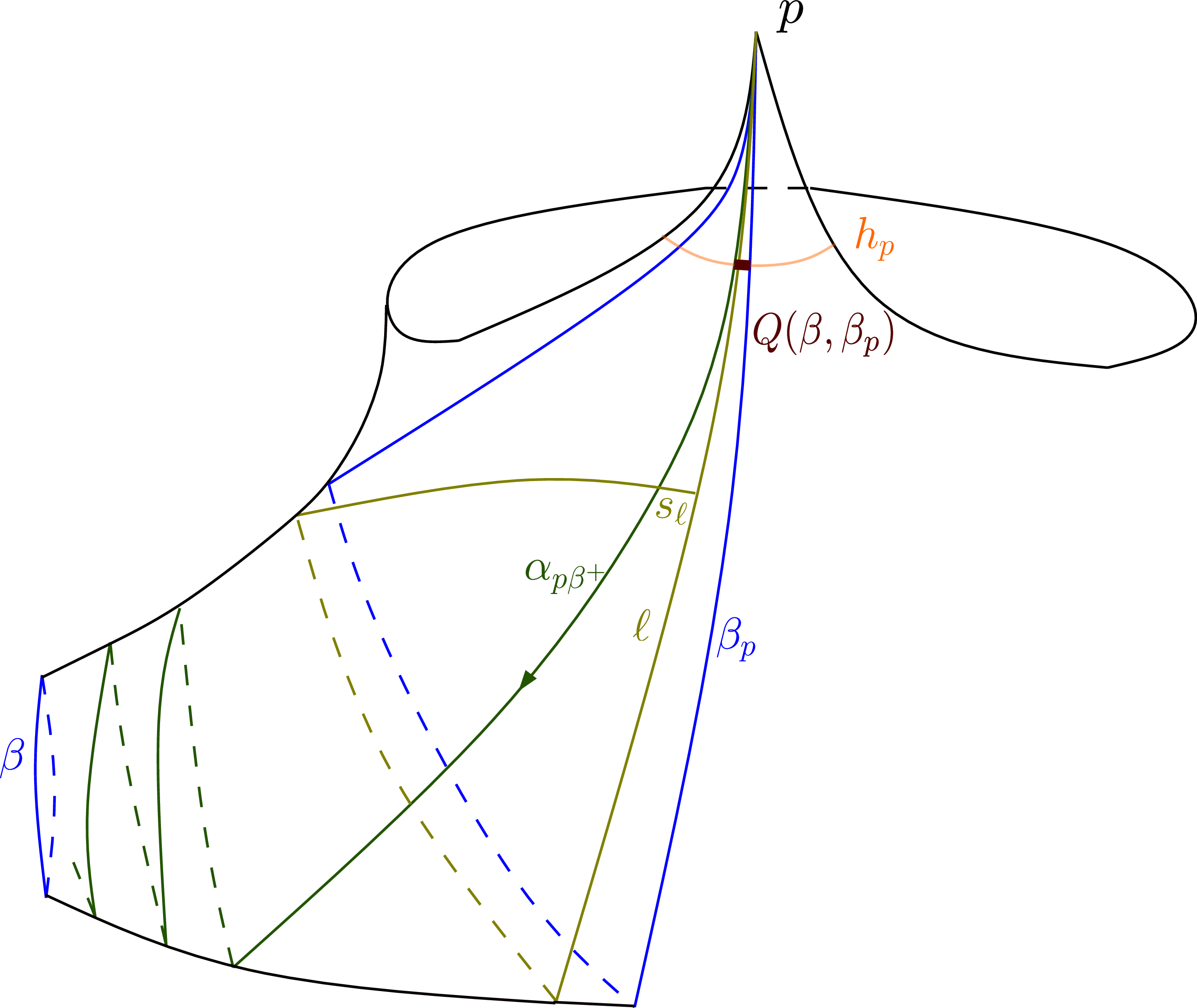
1. Suppose that the geodesic \(\ell\) is self-intersecting. We describe the limiting behavior of geodesics following the argument around [15]. Denote by \(s_\ell\) the first self-intersection point on \(\ell\). Consider the loop \(\alpha_\ell\) on \(\ell\) going from \(s_\ell\) to itself, see Figure 21. It is homotopic to a simple closed geodesic \(\beta\). When \(\ell\) moves towards the \(\beta\), the geodesic \(p s_\ell\), obtained by moving from \(p\) along \(\ell\) to the first self-intersection at the point \(s_\ell\), converges to a bi-infinite geodesic \(\alpha_{p\beta^+}\) spiraling around \(\beta\) infinitely many times. It provides an orientation of \(\beta\). When \(\ell\) moves in the opposite direction, the loop \(\alpha_\ell\) does not change its homotopy class till \(\ell\) converges to some bi-infinite geodesic \(\beta_p\). The geodesic \(\beta_p\) is the limit of both loop \(\alpha_\ell\) and the path \(p s_\ell\). We denote by \(Q(\beta,\beta_p)\) the gap, defined as the length of the horoarc between the intersection points of the two bi-infinite geodesics \(\alpha_{p\beta^+}\) and \(\beta_p\) with the horocycle \(h_p\). On the other hand, the ideal triangle bounded by \((\alpha_{p\beta^+}, \beta_p)\) lifts to some \((\tilde{p},\beta^+, \beta \tilde{p})\) in the universal cover. Suppose the decoration \(v_p\) at \(\tilde{p}\) is the same as the decoration at \(p\), the framing at \(\beta^+\) and \(\beta \tilde{p}\) can be obtained by parallel transporting \(\left<v_p\right>\) along \(\alpha_{p\beta^+}\) and \(\beta_p\) respectively. Then we define the potential \(W_p(\alpha_{p\beta^+}, \beta_p)\) by equation 40 . By (73 ), the gap is equal to the value of the potential \(W_p(\alpha_{p\beta^+}, \beta_p)\). The geodesics \(\beta\) and \(\beta_p\) bounds an embedded trouser leg, see Figure 22, which is denoted by \[{\rm T}(\beta,\beta_p).\] The decorated surface describing the trouser leg is a punctured disc with a marked point, see Figure 23. The pair \((\beta,\beta_p)\) uniquely determines a trouser leg unless we consider the once punctured torus case.11 The isomorphism class of the ideal hyperbolic surface \({\rm T}(\beta, \beta_{p})\) is determined by the length \(l_\beta\) of the neck geodesic and the horocycle length \({\rm K}_{\beta_p}\) of the boundary arc. Let us set \[{\rm L}_\beta:=e^{\l_\beta}.\]
Observe that the gap \(Q(\beta,\beta_p)\) is equal to the potential \(W_p(\alpha_{p\beta^+}, \beta_p)\) \[\label{D=W} Q(\beta,\beta_p) = W_p(\alpha_{p\beta^+}, \beta_p).\tag{74}\]
Lemma 11. The potential \(W_p(\alpha_{p\beta^+}, \beta_p)\) for the trouser leg \({\rm T}(\beta, \beta_p)\) is given by \[\label{551} \begin{align} W_p(\alpha_{p\beta^+}, \beta_p)={\rm K}^{1/2}_{\beta_p} {\rm L}_\beta^{-1/2}.\\ \end{align}\qquad{(21)}\] Therefore the gap \(Q(\beta,\beta_p)\) is given by \[\label{gapfunct} \begin{align} Q(\beta,\beta_p) &={\rm K}^{1/2}_{\beta_p}{\rm L}_\beta^{-1/2}.\\ \end{align}\qquad{(22)}\]
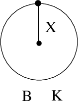
Proof. Denote by \({{\rm B}}, {{\rm X}}\) the cluster Poisson coordinates at the two edges of the decorated surface underlying a trouser leg on Figure 23. Then \[{\rm K}_{\beta_p} = {\rm B}{\rm X}{\rm B}, \quad {\rm L}_\beta = {\rm X}.\] The potential is given by \(W_p(\alpha_{p\beta^+}, \beta_p)={\rm B}_{\beta_p}\). So we get: \[\label{EXVT} \begin{align} W_p(\alpha_{p\beta^+}, \beta_p)&= {\rm K}_{\beta_p}^{1/2}{\rm L}_\beta^{-1/2}.\\ \end{align}\tag{75}\] The second claim follows immediately from this and (74 ). ◻
Remark. By [15], the bi-infinite geodesic \(\beta_p\) uniquely determines the trouser leg \({\rm T}(\beta,\beta_p)\), but \(p\) and \(\beta\) do not determine \(\beta_p\). For example, let \({\rm D}_\delta \gamma_p\) be the Dehn-twist of the bi-infinite geodesic \(\gamma_p\) on Figure 45 around the loop \(\delta\). Then \(\gamma_p \not = {\rm D}_\delta \gamma_p\), but \(\gamma = {\rm D}_\delta \gamma\). The related embedded trouser leg is \({\rm T}(\gamma,{\rm D}_\delta \gamma_p)\). We could also Dehn-twist \(\gamma_p\) around \(\eta\). The Dehn twists around \(\delta\) and \(\eta\) do not commute since they intersect. So the orbit of a trouser leg by the action of the group \({\rm Mod}({\Bbb S})\) can be complicated.
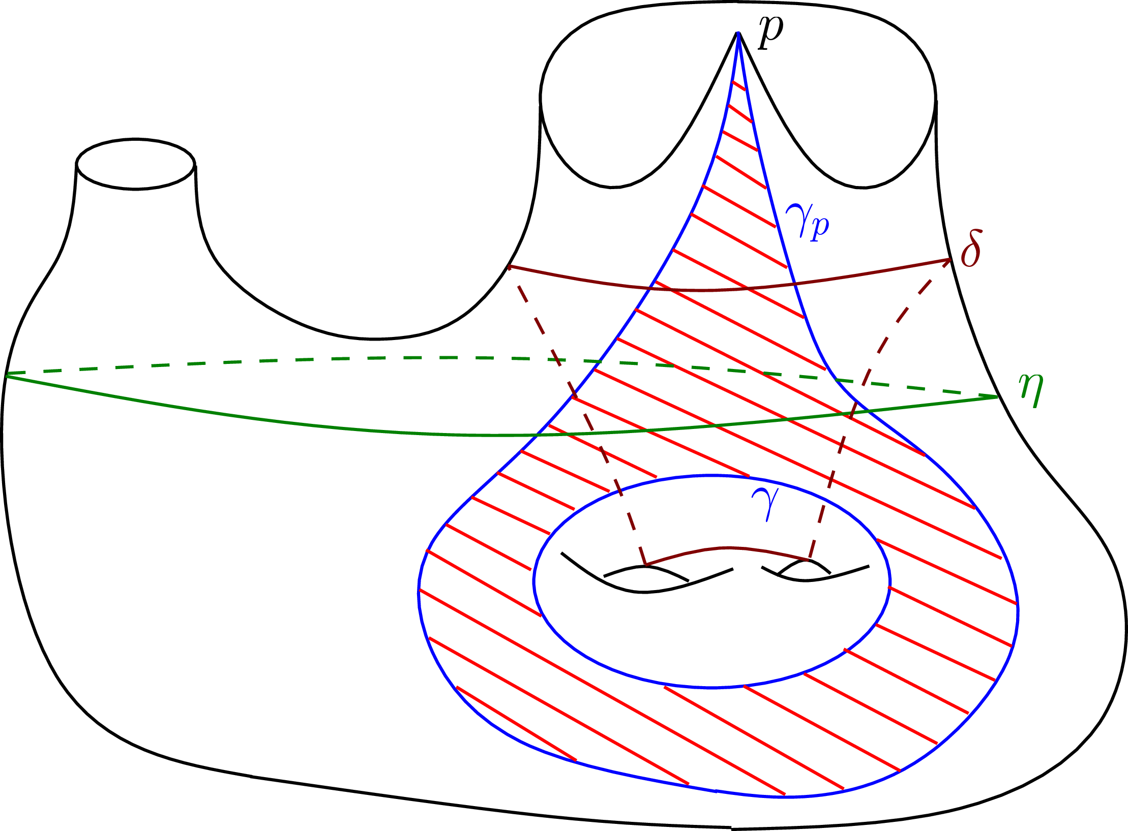
2. Suppose that the simple geodesic \(\ell\) hits the boundary circle \(\beta\) as in Figure 25. If we move \(\ell\) towards the left, it will converge to some simple bi-infinite geodesic \(\alpha_{p\beta^-}\) spiraling around \(\beta^{-}\) - that is \(\beta\) with the opposite orientation - without changing its homotopy class. If we move \(\ell\) towards the right, it will converge to a simple bi-infinite geodesic \(\alpha_{p\beta^+}\) spiraling around \(\beta\) without changing its homotopy class. So there is a unique embedded trouser leg \({\rm T}(\beta,\beta_p)\) containing \(\alpha_{p\beta^-}\) and \(\alpha_{p\beta^+}\).

Let us denote by \(R'(\beta,\beta_p)\) the gap–length of the horoarc between the two bi-infinite geodesics \(\alpha_{p\beta^-}\) and \(\alpha_{p\beta^+}\) intersecting \(h_p\). Then the length of the horoarc on \(h_p\) with the two ends at \(h_p\cap \beta_p\) is \[R(\beta,\beta_p):=R'(\beta,\beta_p)+2Q(\beta,\beta_p).\] Note that this is just the value of the potential \(W_p(\beta, \beta_p)\) at \(p\) for the trouser leg \({\rm T}(\beta, \beta_p)\): \[\label{R=W} R(\beta,\beta_p)=W_p(\beta, \beta_p).\tag{76}\]
Lemma 12. The potential \(W_p(\beta, \beta_p)\) for the trouser leg \({\rm T}(\beta, \beta_p)\) is given by \[\label{EXVT} \begin{align} W_p(\beta, \beta_p) ={\rm K}^{1/2}_{\beta_p}\cdot ({\rm L}_\beta^{-1/2}+{\rm L}_\beta^{1/2}).\\ \end{align}\qquad{(23)}\] Therefore we have \[\label{5511} \begin{align} R(\beta,\beta_p)={\rm K}^{1/2}_{\beta_p}\cdot ({\rm L}_\beta^{-1/2}+{\rm L}_\beta^{1/2}).\\ \end{align}\qquad{(24)}\]
Proof. We use the same notation as in the proof of Lemma 11. Then the potential is given by \(W_p(\beta, \beta_p) = {\rm B}_{\beta_p} + {\rm B}_{\beta_p} {\rm X}\). So it is calculated in terms of the parameters \({\rm K}_{\beta_p}\) and \(l_\beta\) just by (75 ). The second claim follows from this and (76 ). ◻
We observe that this implies the following formula: \[R'(\beta,\beta_p) = {\rm K}_{\beta_p}^{1/2}({\rm L}_\beta^{1/2}-{\rm L}_\beta^{-1/2}).\]
3. Suppose that the simple geodesic \(\ell\) hits the boundary arc \(ab\) of some crown end as in Figure 26. If we move \(\ell\) towards the left, then it will converge to some simple bi-infinite geodesic \(\alpha_{pa}\) without changing its homotopy class. Moving \(\ell\) towards the right, it will converge to some simple bi-infinite geodesic \(\alpha_{pb}\) without changing its homotopy class. Thus we get an embedded ideal triangle \(\tau(\alpha_{pa}, \alpha_{pb})\), with the geodesic sides \(\alpha_{pa}\), \(\alpha_{pb}\) and \(ab\). Denote the gap–length of the horoarc between the two bi-infinite geodesics intersecting \(h_p\) by \(S(\alpha_{pa},\alpha_{pb})\). It is equal to the potential \(W_{p}(\alpha_{pa},\alpha_{pb})\). Let \(v_p, v_a, v_b\) be the decoration vectors at the vertices \(p, a, b\) of the ideal triangle, see Figure 27. Then \[\label{Sfunct} S(\alpha_{pa},\alpha_{pb}) = W_{p}(\alpha_{pa},\alpha_{pb}) = \frac{\omega(v_a, v_b)}{\omega(v_p, v_a) \omega(v_p, v_b)} = \Bigl(\frac{{\rm K}_p}{{\rm K}_a{\rm K}_b}\Bigr)^{-1/2}.\tag{77}\]
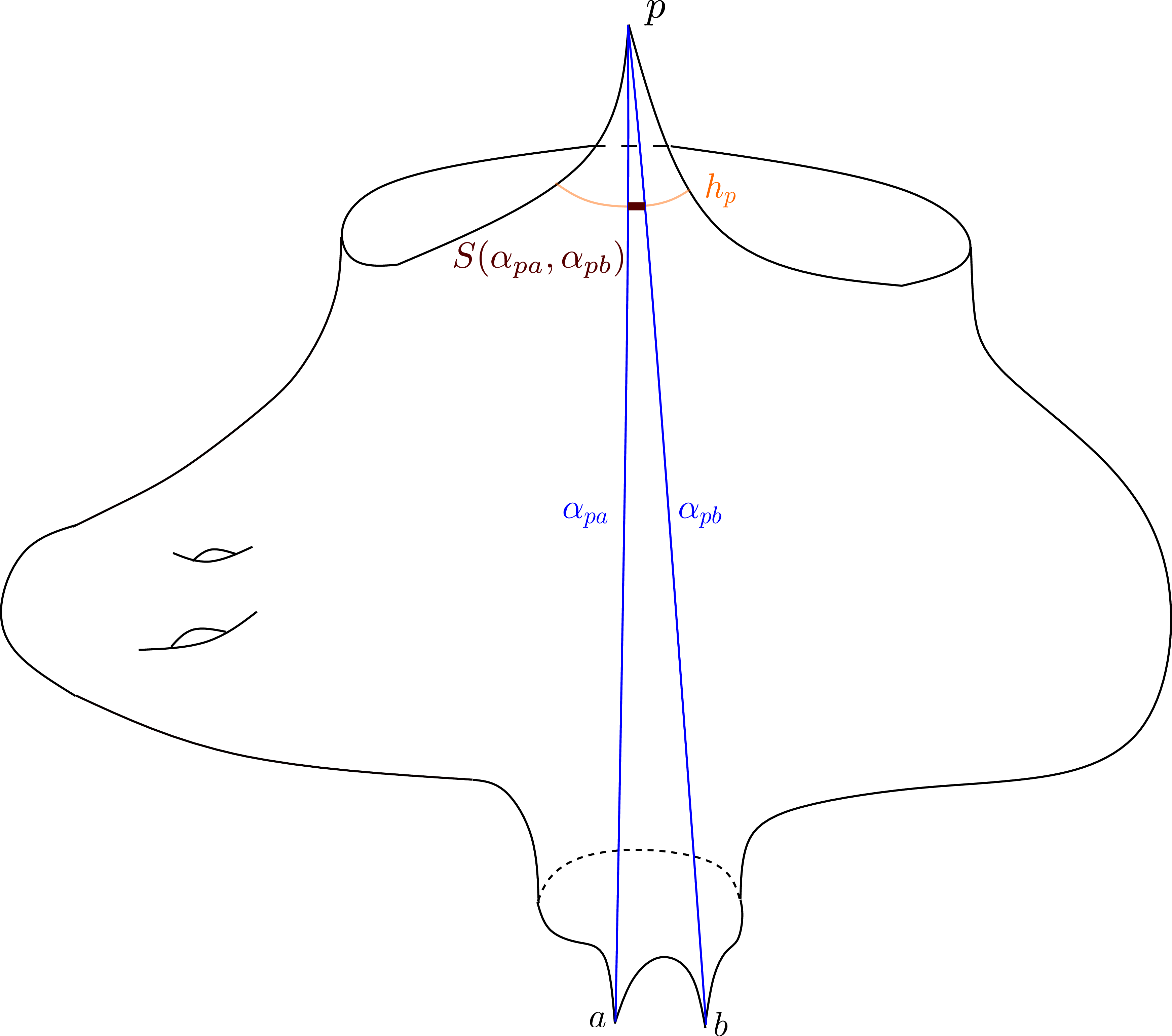
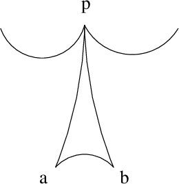
Definition 11. An embedded ideal triangle \(\tau(\alpha_{pa},\alpha_{pb})\) is \(p\)-narrowest* if any cusp region at \(p\) of any other embedded ideal triangle can not be embedded into the cusp region at \(p\) of \(\tau(\alpha_{pa},\alpha_{pb})\).*
An ideal geodesic triangle \(\tau\) id \(p\)-narrowest if and only if its opposite side \(ab\) is a bi-infinite boundary geodesic. So it connects two adjacent cusps on the same crown \(\rm C\). The vertices \(a\) and \(b\) coincide if and only if the crown \(\rm C\) has a single cusp, as shown on the right of Figure 28. The opposite side \(ab\) can be at the same crown as the cusp \(p\). The three vertices of the triangle \(\tau\) can coincide, as shown on Figure 8.
There are the following sets of elementary decorated surfaces containing the chosen cusp \(p\):
The set \({\cal H}_{{\rm T}, p}\) of isotopy classes of trouser legs \({\rm T}\) containing \(p\). It is a union of two disjoint subsets: \[{\cal H}_{{{\rm T}}, p} ={\cal H}^{\partial}_{{{\rm T}}, p}\cup ({\cal H}_{{{\rm T}}, p}-{\cal H}^{\partial}_{{{\rm T}}, p}).\] Here \({\cal H}^{\partial}_{{{\rm T}}, p}\) is the subset where \(\ell_{\rm T}\subset \partial {\Bbb S}\): the geodesic boundary loop \(\ell_{\rm T}\) lies on the boundary of \({\Bbb S}\).
The set \({\cal H}_{{\tau}, p}\) of isotopy classes of ideal \(p\)-narrowest triangles triangles \(\tau\) containing the cusp \(p\). It is a union of two disjoint subsets, depending how many internal sides has the triangle \(\tau\): one or two: \[{\cal H}_{{\tau}, p} ={\cal H}^{(1)}_{{\tau}, p}\cup {\cal H}^{(2)}_{{\tau}, p}.\]
Let us state the McShane identity for a cusp/puncture \(p\) on an ideal hyperbolic surface.
Recall the local potential \(W_p\) at cusp \(p\).
Theorem 23. Given an ideal hyperbolic surface, given a cusp \(p\) at a crown or a puncture \(p\), we get \[\label{MSRF2} \sum_{\rm{T}(\beta,\beta_p) \in {\mathcal{H}}_{T, p} - {\mathcal{H}}_{T, p}^{\partial}} 2 Q(\beta,\beta_p)+\sum_{{\rm T}(\beta,\beta_p)\in {\mathcal{H}}_{T, p}^\partial}R(\beta,\beta_p)+ \sum_{\tau(\alpha_{pa},\alpha_{pb})\in {\cal H}_{\tau, p} }S(\alpha_{pa},\alpha_{pb})=W_p.\qquad{(25)}\]
Proof. It follows immediately from the above construction and Birman–Series [22] theorem, adapted to the surfaces with crowns in Theorem 34. Indeed, the sum of the horoarc lengths of all intervals on the horoarc \(h_p\) involved in the sum is the horocycle length \({\rm H}_p\) of the horoarc \(h_p\). Note that \({\rm H}_p=W_p\). Observe that for non-boundary geodesics \(\beta\), the term \({\cal D}(\beta,\beta_p)\) appears twice: for the trouser leg which orients the geodesic \(\beta\) one way, and for another trouser leg where \(\beta\) is oriented the other way. ◻
4.0.0.1 Remarks.
1. On Figure 28 (1) for the ideal triangle \(\tau(\alpha_{pa},\alpha_{pb})\), the potential \(W_{p}(\alpha_{pa},\alpha_{pb})\) is the sum of potentials \(W_{p}(\alpha_{pa},\ell)\) and \(W_{p}(\ell,\alpha_{pb})\) for the two smaller ideal triangles. Counting potentials \(W_{p}(\alpha_{pa},\alpha_{pb})\), \(W_{p}(\alpha_{pa},\ell)\) and \(W_{p}(\ell,\alpha_{pb})\) doubles the horoarc length count for potential \(W_{p}(\alpha_{pa},\alpha_{pb})\).
2. On Figure 28 (2) the ideal triangle \(\tau(\ell, \alpha_{pb})\) lies inside of the cylinder bounded by \(\ell_1\) and \(C_b\). Counting potentials \(W_{p}(\ell,\alpha_{pb})\) and \(W_{p}(\alpha_{pa},\alpha_{pb})\) doubles the horoarc length count for the \(W_{p}(\ell,\alpha_{pb})\).
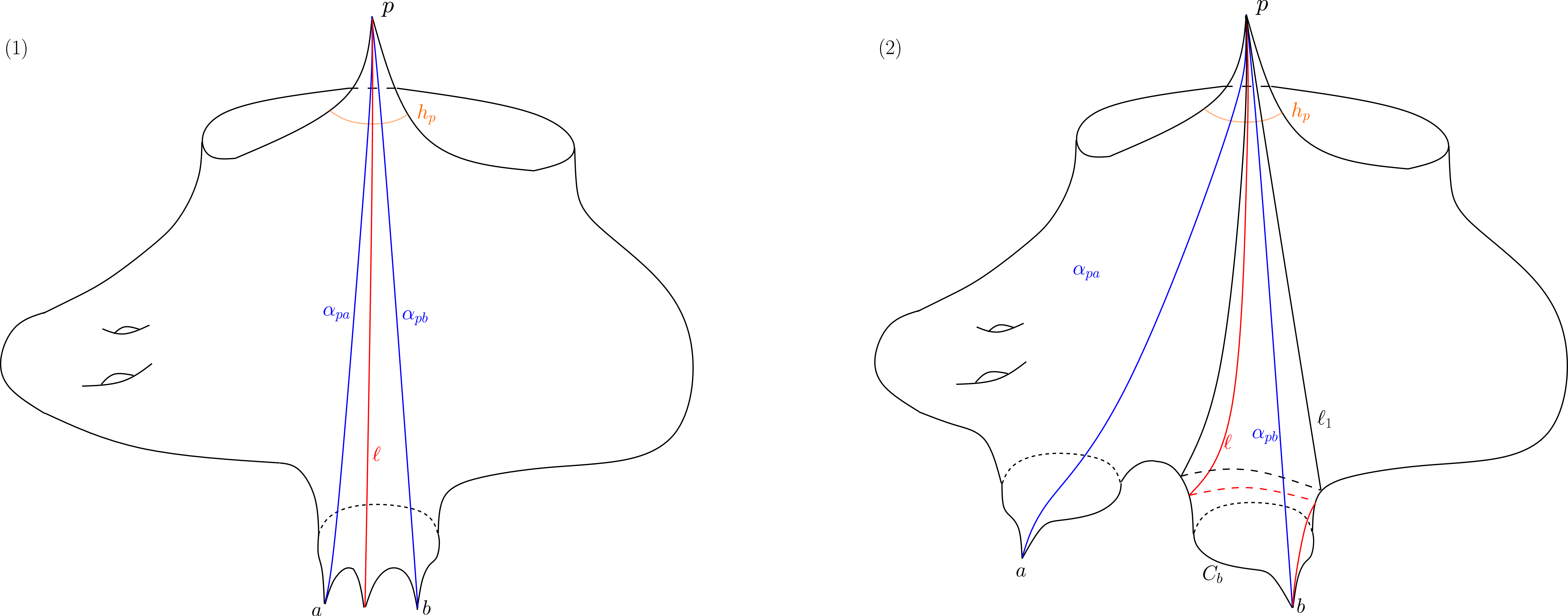
5 The unfolding formula↩︎
5.1 Geometry of unfolding at the cusp \(p\).↩︎
Let us equip \({\Bbb S}\) with an ideal hyperbolic structure. Then we refer to a trouser leg or an ideal triangle on \({\Bbb S}\) as a geodesic trouser leg and ideal geodesic triangle, respectively.
1. Take an ideal geodesic triangle \(\tau\), and cut \({\Bbb S}\) along the \(\tau\): \[{\Bbb S}= ({{\Bbb S}-\tau}) \cup \tau.\] If \(\tau\) has two internal sides, then the \({\rm K}-\)coordinates \(({\rm K}_a, {\rm K}_b)\) at the sides of \({\Bbb S}-\tau\) and \(\tau\) corresponding to them provide two projections: \[{\cal T}_{{{\Bbb S}-\tau}} \longrightarrow({\mathbb{R}}_{+}^\ast)^2, \qquad {\cal T}_{{\tau}} \longrightarrow({\mathbb{R}}_{+}^\ast )^2.\] Consider their fibered product \({\cal T}_{{{\Bbb S}-\tau}} \times_{({\mathbb{R}}_{+}^\ast)^2} {\cal T}_{{\tau}}.\) It comes with the canonical projection \[({\rm K}_a, {\rm K}_b):{\cal T}_{{{\Bbb S}-\tau}} \times_{({\mathbb{R}}_{+}^\ast)^2} {\cal T}_{{\tau}} \longrightarrow({\mathbb{R}}_{+}^\ast)^2.\]
If the triangle \(\tau\subset {\Bbb S}\) has a single internal side, there is a similar fibered product with the projection \[{\rm K}_a:{\cal T}_{{{\Bbb S}-\tau}} \times_{{\mathbb{R}}_{+}^\ast } {\cal T}_{{\tau}} \longrightarrow{\mathbb{R}}_{+}^\ast.\] Let \({\rm Stab}_\tau\subset {\rm Mod}({\Bbb S})\) be the subgroup stabilizing the triangle \(\tau\). One has \[\label{gr1} {\rm Stab}_{\tau} = {\rm Mod}({{\Bbb S}- \tau}).\tag{78}\]
Proposition 24. Cutting \({\Bbb S}\) along the \(k\) sides of an ideal triangle \(\tau\) provides an isomorphism \[\label{itau} i_\tau: {\cal T}_{{\Bbb S}} \stackrel{\sim}{\longrightarrow} {\cal T}_{{\Bbb S}-\tau}\times_{({\mathbb{R}}^\ast_{+})^k} {\cal T}_{\tau} .\qquad{(26)}\] It is equivariant under the action of the group \({\rm Stab}_\tau\). One has \[\label{118} \begin{align} &i_\tau^*\Omega_{\Bbb S}({\rm K}, {\rm L}) = \Omega_{{\Bbb S}-\tau}({\rm K}', {\rm L}) \wedge d\log {\rm K}_a\wedge d\log {\rm K}_b; \;\;if k=2\\ &i_\tau^*\Omega_{\Bbb S}({\rm K}, {\rm L}) = \Omega_{{\Bbb S}-\tau}({\rm K}', {\rm L}) \wedge d\log {\rm K}_a; \;\;\; \;\;\; \;\;\;\;\;\;\;\;\;if k=1.\\ &i_\tau^*W_{\Bbb S}= W_{{\Bbb S}-\tau} + W_\tau.\\ \end{align}\qquad{(27)}\]
Passing to the quotient by the action of the group (78 ) we get an isomorphism \[\label{isotau2} {\cal M}_{{\Bbb S}-\tau}\times_{({\mathbb{R}}^\ast_{+})^k} {\cal M}_{\tau} \stackrel{\sim}{\longrightarrow} {\cal M}_{{\Bbb S}, \tau}:= {\cal T}_{{\Bbb S}}/{\rm Stab}_\tau.\tag{79}\] There is the unfolding map: \[{\cal M}_{{\Bbb S}, \tau} = {\cal T}_{{\Bbb S}}/{\rm Stab}_\tau\; \longrightarrow\;{\cal M}_{{\Bbb S}} = {\cal T}_{{\Bbb S}}/{\rm Mod}({{\Bbb S}}).\]
2. Similarly, take a trouser leg \({\rm T}\subset {\Bbb S}\) with the sides \(({\rm F}, \ell_{\rm T})\), and cut the surface \({\Bbb S}\) along the \({\rm T}\): \[{\Bbb S}= ({{\Bbb S}-{\rm T}}) \cup {\rm T}.\] Recall the Fenchel–Nielsen length-twist coordinates \((l,\theta)\) related to the loop \(\ell_{\rm T}\). The \({\rm K}-\)coordinate and the length \(l\) of the matching boundary components of \({{\Bbb S}-{\rm T}}\) and \({\rm T}\) provide projections \[({\rm K}, l): {\cal T}_{{{\Bbb S}-{\rm T}}} \longrightarrow{\mathbb{R}}_{+}^\ast\times {\mathbb{R}}_{+}, \qquad ({\rm K}, l): {\cal T}_{{{\rm T}}} \longrightarrow{\mathbb{R}}_{+}^\ast \times {\mathbb{R}}_{+}.\] Let us consider their fibered product: \[{\cal T}_{{{\Bbb S}-{\rm T}}} \times_{({\mathbb{R}}_{+}^\ast\times {\mathbb{R}}_{+})} {\cal T}_{{{\rm T}}}.\] The subgroup \({\rm Stab}_{{\rm T}}\) stabilizing \({\rm T}\) contains the Dehn twist \({\rm D}_\ell\) along the loop \(\ell\), acting by \((l, \theta)\longmapsto(l, \theta+l)\), and the subgroup \({\rm Mod}({{\Bbb S}-{\rm T}})\), commuting with the Dehn twist. They generate the group \({\rm Stab}_{{\rm T}}\): \[{\rm Stab}_{{\rm T}} = \langle {\rm D}_\ell\rangle \times {\rm Mod}({{\Bbb S}-{\rm T}}).\]
Lemma 13. Cutting \({\Bbb S}\) along a trouser leg \({\rm T}=(a,\ell_T)\subset {\Bbb S}\) provides a \({\rm Mod}({{\Bbb S}- {\rm T}})\)-equivariant map \[\label{SPT} \begin{align} &i_{\rm T}: {\cal T}_{{\Bbb S}} \stackrel{{\mathbb{R}}}{\longrightarrow} {\cal T}_{{\Bbb S}-{\rm T}}\times_{({\mathbb{R}}^\ast_{+}\times{\mathbb{R}}_{+})} {\cal T}_{{\rm T}}, \;\;\;\;if \ell_{\rm T}\not \subset \partial {\Bbb S};\\ &i_{\rm T}: {\cal T}_{{\Bbb S}} \stackrel{\sim}{\longrightarrow} {\cal T}_{{\Bbb S}-{\rm T}}\times_{{\mathbb{R}}^\ast_{+}} {\cal T}_{{\rm T}} \;\;\;\;\;\; \;\;\;\;\;\;if \ell_{\rm T}\subset \partial {\Bbb S}.\\ \end{align}\qquad{(28)}\] It is a principal \({\mathbb{R}}-\)fibration parametrised by the twist parameter \(\theta\) in the first case, and an isomorphism in the second. Recall \(c_{{\Bbb S},\ell_T}\) in Proposition 17 One has \[\label{SPT1} \begin{align} &i_{\rm T}^* \Omega_{\Bbb S}({\rm K}, {\rm L})=c_{{\Bbb S},\ell_T}\cdot \Omega_{{\Bbb S}-{\rm T}}({\rm K}',{\rm L}') \wedge dl \wedge d\theta \wedge d\log {\rm K}_a\;\;\;\;if \ell_{\rm T}\not \subset \partial {\Bbb S};\\ &i_{\rm T}^* \Omega_{\Bbb S}({\rm K}, {\rm L})= \Omega_{{\Bbb S}-{\rm T}}({\rm K}',{\rm L}) \wedge d\log {\rm K}_a \;\;\;\;\; \;\; \;\;\;\;\;\; \;\;if \ell_{\rm T}\subset \partial {\Bbb S}.\\ &i_{\rm T}^*W_{\Bbb S}= W_{{\Bbb S}-{\rm T}} + W_{\rm T}.\\ \end{align}\qquad{(29)}\]
Proof. The claims (?? ) are the standard properties of the Teichmuller spaces. Proposition 15 and Proposition 17 imply the first line in equation (?? ). The last two lines in (?? ) follow from Proposition 15 and Lemma 8. ◻
After the quotient by the action of the group \({\rm Stab}_{\rm T}\), the map \(i_{\rm T}\) provides an \(S^1-\)fibration \[\label{opp} {\cal M}_{{\Bbb S}, {\rm T}}:= {\cal T}_{{\Bbb S}}/{\rm Stab}_{\rm T}\stackrel{S^1}{\longrightarrow} {\cal M}_{{\Bbb S}-{\rm T}}\times_{({\mathbb{R}}^\ast_{+}\times {\mathbb{R}}_+)} {\cal M}_{{\rm T}}.\tag{80}\]
Passing to the quotient by \({\rm Mod}({\Bbb S})\) we get the unfolding map \({\cal M}_{{\Bbb S}, {\rm T}}\longrightarrow{\cal M}_{{\Bbb S}}\).
Recall the exponential volume form \[{\Bbb E}_{\Bbb S}= \;e^{-W_{\Bbb S}}\;\Omega_{\Bbb S},\] and (18 ). Therefore (?? ) and Proposition 16 \(\&\) (?? ) imply the factorization property of exponential volume forms under the cutting of \({\Bbb S}\): \[\label{FEV} \begin{align} &i_\tau^*{\Bbb E}_{\Bbb S}= {\cal E}_{\tau} \cdot {\Bbb E}_{{\Bbb S}-\tau} \wedge d\log {\rm K}_a \wedge d\log {\rm K}_b \;\;if k=2;\\ &i_\tau^*{\Bbb E}_{\Bbb S}= {\cal E}_{\tau} \cdot {\Bbb E}_{{\Bbb S}-\tau} \wedge d\log {\rm K}_a \; \qquad \qquad \quad if k=1;\\ &i_{\rm T}^*{\Bbb E}_{\Bbb S}= c_{{\Bbb S},\gamma}\cdot {\cal E}_{{\rm T}}\cdot {\Bbb E}_{{\Bbb S}-{\rm T}} \wedge dl \wedge d\theta \wedge d\log {\rm K}_a;\\ &i_{\rm T}^*{\Bbb E}_{\Bbb S}= {\cal E}_{{\rm T}}\cdot {\Bbb E}_{{\Bbb S}-{\rm T}} \wedge d\log {\rm K}_a.\\ \end{align}\tag{81}\]
Summarizing, we have the following spaces, highlighting the base coordinates: \[\label{FP31} \begin{align} &{\cal M}_{{\Bbb S}, {\rm T}}({\rm K}_a, l, \theta)\stackrel{S^1}{\longrightarrow}{\cal M}_{{\Bbb S}-{\rm T}}\times_{({\mathbb{R}}^\ast_{+}\times {\mathbb{R}}_+)} {\cal M}_{{\rm T}}, \qquad ({\rm K}_a,l, \theta) \in {\mathbb{R}}^\ast_{+}\times {\mathbb{R}}_+\times S^1,\ell_{\rm T}\not \subset \partial{\Bbb S};\\ &{\cal M}_{{\Bbb S}, {\rm T}}({\rm K}_a)\stackrel{\sim}{\longrightarrow}{\cal M}_{{\Bbb S}-{\rm T}}\times_{{\mathbb{R}}^\ast_{+}} {\cal M}_{{\rm T}}, \qquad \; \;\;\qquad \;\;\;\;{\rm K}_a \in {\mathbb{R}}^\ast_{+}, \quad \; \;\;\;\;\;\;\;\ell_{\rm T}\subset \partial{\Bbb S};\\ &{\cal M}_{{\Bbb S}, {\tau}}({\rm K}_a, {\rm K}_b)\stackrel{\sim}{\longrightarrow} {\cal M}_{{\Bbb S}-\tau}\times_{({\mathbb{R}}^\ast_{+})^2} {\cal M}_{\tau}, \qquad\;\; \; \quad {\rm K}_a,{\rm K}_b \in ({\mathbb{R}}^\ast_{+})^2, \quad k=2;\\ &{\cal M}_{{\Bbb S}, {\tau}}({\rm K}_a)\stackrel{\sim}{\longrightarrow} {\cal M}_{{\Bbb S}, \tau}\times_{{\mathbb{R}}^\ast_{+}} {\cal M}_{\tau}, \qquad\;\;\; \;\quad \qquad \; \;{\rm K}_a \in {\mathbb{R}}^\ast_{+}, \qquad \qquad k=1. \\ \end{align}\tag{82}\] Let us now elaborate Theorem 6. Let \(d_{\rm T}\) be \(\frac{1}{2}\) if \({\rm T}\) is cutting off a one-holed torus, or \(1\) otherwise.
Theorem 25. For any decorated surface \({\Bbb S}\) and a crown with a single cusp \(p\), and any smooth function \(f\) on the moduli space \({\cal M}_{\Bbb S}({{\rm K}}, {\rm L})\), we have the unfolding formula \[\label{recur} \begin{align} &\int _{{\cal M}_{\Bbb S}({{\rm K}}, {\rm L})}f \;W_p\;{\Bbb E}_{\Bbb S}=\\ &\sum_{{{\rm T}}} \int_{ {\cal M}_{{\Bbb S}, {{\rm T}}}({\rm K},{\rm L},{\rm K}_a)} f\cdot (e^{-W_{\rm T}} W_{{\rm T}})({\rm K}_a, l, \theta)\cdot \; {\Bbb E}_{{\Bbb S}-{\rm T}} \wedge d\log {\rm K} \\ &+\sum_{{{\rm T}} } c_{{\Bbb S},\gamma} d_{\rm T}\cdot \int_{ {\cal M}_{{\Bbb S}, {\rm T}}({\rm K}, {\rm L}, l,{\rm K}_a) } f\cdot (e^{-W_{\rm T}}Q_{\rm T})({\rm K}_a, l, \theta)\cdot \;{\Bbb E}_{{\Bbb S}-{{\rm T}}} \wedge dl \wedge d\theta\wedge d\log {\rm K}_a\\ &+\sum_{{\tau_1} } \int_{ {\cal M}_{{\Bbb S}, \tau_1}({\rm K}_a)} f\cdot (e^{-W_\tau } W_{\tau_1, p})({\rm K}_a, {\rm K}_b, {\rm K}_p) \cdot \; {\Bbb E}_{{\Bbb S}-\tau_1} \wedge d\log {\rm K}_a\\ &+\sum_{{\tau_2} } \int_{ {\cal M}_{{\Bbb S}, \tau_2}({\rm K}_a, {\rm K}_b)} f\cdot(e^{-W_\tau } W_{\tau_2, p})({\rm K}_a, {\rm K}_b, {\rm K}_p) \cdot \; {\Bbb E}_{{\Bbb S}-\tau_2} \wedge d\log {\rm K}_a\wedge d\log {\rm K}_b.\\ \end{align}\qquad{(30)}\]
The first (respectively the second) sum is over topological types of embedded trouser legs \({{\rm T}}\) containing \(p\), where \(\ell_{\rm T}\subset \partial {\Bbb S}\) (respectively \(\ell_{\rm T}\not \subset \partial {\Bbb S}\)).
The third (respectively the fourth) sum is over topological types of the embedded \(p\)-narrowest ideal triangles \(\tau\) containing \(p\) with a single internal side (respectively with two internal sides).
Remark 26.

Let us denote the decorated surface \({\Bbb S}\) by \(S_{g,m;n_1,...,n_r}\) where the number of boundary components is \(m\) and the crowns \({\rm C}_i\) is of type \(n_i\). There are several cases of the surface after cutting off a trouser leg or a \(p\)-narrowest ideal triangle.
When we cut off a trouser leg \({\rm T}\) from the surface \({\Bbb S}\) as in Figure (1),
if the boundary circle \(\ell_{\rm T}\) of \({\rm T}\) is also contained in the boundary of \({\Bbb S}\), in this case the ideal edge \(a\) is connected to the crown of type \(n_1\) through the cusp \(p\). Thus \({\Bbb S}-{\rm T}=S_{g,m-1;n_1+1,n_2,...,n_r}\) and it corresponds to the second line of formula (?? );
if \({\Bbb S}-{\rm T}\) is connected and the boundary circle \(\ell_{\rm T}\) is not contained in the boundary of \({\Bbb S}\), the left side and the right side of Figure 29 (1) is connected somewhere. Cutting off \({\rm T}\) will decrease the genus \(g\) by \(1\), increse the number of boundary components \(m\) by \(1\), and change the type \(n_1\) crown containing \(p\) into type \(n_1+1\) crown as the last case. Thus \({\Bbb S}-{\rm T}=S_{g-1,m+1;n_1+1,n_2,...,n_r}\) and it corresponds to the part of the third line of formula (?? );
if \({\Bbb S}-{\rm T}\) is not connected, the trouser leg \({\rm T}\) cuts \({\Bbb S}\) into two connected components. Suppose the left side connected component as in Figure 29 (1) is \(S_{g_1,m_1+1;n_{k+1},...,n_r}\), then \({\Bbb S}-{\rm T}=S_{g_1,m_1+1;n_{k+1},...,n_r} \cup S_{g-g_1,m-m_1;n_{1}+1,n_2,...,n_k}\) and it corresponds to the other part of the third line of formula (?? ).
As in Figure (2), the ideal points \(p'\) and \(p''\) could coincide. Moreover \(p, p', p''\) could also coincide, then some of \(n_k\) has to be \(1\), and in this case \({\Bbb S}-\tau\) could be two connected components. When we cut off a \(p\)-narrowest ideal triangle \(\tau\) from the surface \({\Bbb S}\),
if one of the ideal edges \(a\) and \(b\) of \(\tau\) is also contained in the boundary of \({\Bbb S}\) even though the other ideal edge of \(\tau\) is already contained in the boundary of \({\Bbb S}\), then \(\tau\) is contained in some crown of type \(n_1\)(\(n_1\geq 2\)) containing the cusp \(p\). Cutting off \(\tau\) will only change this type \(n_1\) crown into type \(n_1-1\) crown. Thus \({\Bbb S}-\tau=S_{g,m;n_1-1,n_2,...,n_r}\) and it corresponds to the fourth line of formula (?? );
if both of the ideal edges \(a\) and \(b\) are not contained in the boundary of \({\Bbb S}\) and \({\Bbb S}-{\rm T}\) is connected, cutting off the ideal triangle \(\tau\) will combine the two crowns touching \(\tau\) into a single crown. Namely, the type \(n_1\) crown and the type \(n_2\) crown is combined into the type \(n_1+n_2+1\) crown. Thus \({\Bbb S}-\tau=S_{g,m-1;n_1+n_2+1,n_3,...,n_r}\) and it corresponds to the part of the fifth line of formula (?? );
if \({\Bbb S}-\tau\) is not connected, then the ideal triangle \(\tau\) has to be the ideal triangle with a single vertex \(p\) as in Figure 8 and \(\tau\) cuts \({\Bbb S}\) into two connected components. In this case, the crown containing \(p\) is of type \(n_1=1\). Suppose the left side connected component as in Figure 29 (2) is \(S_{g_1,m_1+1;1, n_{k+1},...,n_r}\), then \({\Bbb S}-\tau=S_{g_1,m_1+1;1, n_{k+1},...,n_{r}} \cup S_{g-g_1,m-m_1;1,n_{2},...,n_{k}}\) and it corresponds to the other part of the fifth line of formula (?? ).
5.2 Proof of Theorem 25.↩︎
Proof. Let \(\{\gamma\}=(\gamma_1,..., \gamma_s)\) be a collection of disjoint geodesics, where \(\gamma_1\), \(...\), \(\gamma_{s-s'}\) are simple bi-infinite geodesics and the rest are simple closed geodesics, see Figure 30. Consider a cover \[\label{cov} \pi_{\{\gamma\}}: \mathcal{M}_{{\Bbb S}}({{\rm K}},{{\rm L}}; {\{\gamma\}}) \longrightarrow\mathcal{M}_{{\Bbb S}}({{\rm K}},{{\rm L}})\tag{83}\] given by pairs \((\Sigma, \{\eta\})\), where \(\Sigma\in \mathcal{M}_{{\Bbb S}}({{\rm K}},{{\rm L}})\), and \(\{\eta\}\) is an element of the \({\rm Mod}({\Bbb S})-\)orbit of \(\{\gamma\}\).
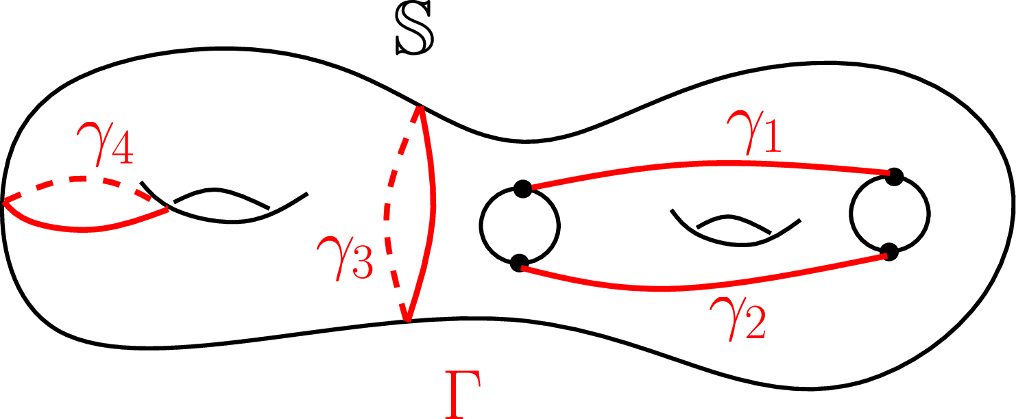
Consider the subgroup of the pure mapping class group stabilising each element of the collection \(\{\gamma\}\): \[{\rm Stab}_{\{\gamma\}} \subset \rm{Mod}({\Bbb S}).\] Then \[\begin{align} &\mathcal{M}_{{\Bbb S}}({{\rm K}}, {\rm L})=\mathcal{T}_{{\Bbb S}}({{\rm K}},{{\rm L}})/{\rm Mod}({\Bbb S}),\\ &\mathcal{M}_{{\Bbb S}, \{\gamma\}}({{\rm K}},{{\rm L}})=\mathcal{T}_{{\Bbb S}}({{\rm K}},{{\rm L}})/{\rm Stab}_{\{\gamma\}}.\\ \end{align}\] Given an integrable function \(f\) on \(\mathcal{M}_{{\Bbb S}, \{\gamma\}}({{\rm K}},{{\rm L}})\), let \(\pi_{\{\gamma\} \ast}f\) be its push forward by the map (83 ). Then \[\label{0011} \int_{\mathcal{M}_{{\Bbb S}}({{\rm K}},{{\rm L}})}\pi_{\{\gamma\} \ast}f \; {\rm{d} Vol} = \int_{\mathcal{M}_{{\Bbb S}, \{\gamma\}}({{\rm K}},{{\rm L}})} f \;\rm{d} Vol.\tag{84}\]
The two interesting cases of the collection \(\{\gamma\}\) are:
(1) The \(k\) internal sides of an ideal triangle \(\tau\), which has a vertex at the cusp \(p\). Here \(k=1\) or \(2\). (2) The boundary of a trouser leg \(\rm T\). So it is the union of a bi-infinite geodesic and a geodesic loop.
We integrate the function \(fW_p\) over the moduli space \({\cal T}_{\Bbb S}({{\rm K}}, {\rm L})/{\rm Mod}({\Bbb S})\) over the exponential measure: \[\int _{{\cal T}_{\Bbb S}({{\rm K}}, {\rm L})/{\rm Mod}({\Bbb S})}f \;W_p\;{\Bbb E}_{\Bbb S}.\] Using McShane identity (?? ), we present \(W_p\) as a finite collection of sums corresponding to the topological types of the ideal triangles \(\tau\) and trouser legs \({\rm T}\) containing the cusp \(p\). Each of these sums is over a \({\rm Mod}({\Bbb S})-\)orbit of such a \(\tau\) or \({\rm T}\). Now we have several cases to consider.
1. Take the sum over the orbit of an ideal triangle \(\tau\). The triangle can have two or one internal edges.
(\(1'\)) Let \(\{\tau\}=\ell_a\cup\ell_b\) be the union of two ideal edges of \(\tau\) other than the boundary edge. Recall \[\left|\mathrm{Stab}_{\{\tau\}}/\left(\mathrm{Stab}_{\ell_a}\cap \mathrm{Stab}_{\ell_b}\right)\right|=1.\] Then by [13] \[\sum_{\alpha\in \mathrm{Mod}({\Bbb S})\{\tau\}} f= \pi_{\{\tau\} \ast}f.\]
It can be written as a single integral over the unfolding cover \[\pi_{\tau}: {\cal M}_{{\Bbb S}, \tau}\longrightarrow{\cal M}_{{\Bbb S}}\] of the product of the function \(f\) by the potential function \(W_{\tau, p} = S(\alpha_{pa},\alpha_{pb})\): \[\int _{{\cal T}_{\Bbb S}({{\rm K}}, {\rm L})/ {\rm Stab}_\tau}f \;W_{\tau,p}\;{\Bbb E}_{\Bbb S}.\] Using the isomorphism \(i_\tau\) in (?? ), and since \(k=2\) in the (\(1')\) case, we can write it as \[\label{opp1} \begin{align} &\int _{ {\cal T}_{{\Bbb S}-\tau}\times_{({\mathbb{R}}^\ast_{+})^2} {\cal T}_{\tau} / {\rm Stab}_\tau}f \;W_{\tau,p}\;i_\tau^*({\Bbb E}_{\Bbb S}) \\ \stackrel{(\ref{isotau2})}{=}& \int _{ {\cal M}_{{\Bbb S}-\tau}\times_{({\mathbb{R}}^\ast_{+})^2} {\cal M}_{\tau}}f \;W_{\tau,p}\;i_\tau^*({\Bbb E}_{\Bbb S})\\ \stackrel{(\ref{FEV})}{=}& \int _{ {\cal M}_{{\Bbb S}-\tau}\times_{({\mathbb{R}}^\ast_{+})^2} {\cal M}_{\tau}}f e^{-W_\tau}\;W_{\tau,p}\;{\Bbb E}_{{\Bbb S}-\tau} \wedge d\log {\rm K}_a \wedge d\log {\rm K}_b.\\ \end{align}\tag{85}\]
The bottom line here is exactly the bottom line in formula (?? ).
(\(1''\)) The same argument for the ideal triangles \(\tau\) with a single internal side gives the last line in (?? ).
2. Take the sum over the orbit of a trouser leg \({\rm T}\). It can be written as a single integral over the unfolding cover \[\pi_{{\rm T}}: {\cal M}_{{\Bbb S}, {\rm T}}\longrightarrow{\cal M}_{{\Bbb S}}\] of the product of the function \(f\) by either the function \({\cal Q}_{{\rm T}}\) or \({W}_{\rm T}\). By [13], the factor \(d_{{\rm T}}\) comes from the hyperelliptic evolution of the one-holed torus cut out from the closed geodesic of the touser leg \({\rm T}\). The rest of the argument follows the same lines as above, using (80 ) instead of (79 ) in (85 ). Theorem 25 is proved. ◻
5.3 The reduced unfolding formula.↩︎
Given a crown with a single cusp \(p\), there is a canonical trouser leg \({\rm T}_p^\sharp\) for which the boundary geodesic loop is the neck geodesic for the crown. The trouser leg \({\rm T}_p^\sharp\) is preserved by the mapping class group \({\rm Mod}({\Bbb S})\). All other trouser legs at the cusp \(p\) have infinite orbits under the mapping class group action. So the related terms in the unfolding formula are integrals over moduli spaces which are simpler than the original one. However this is not the case for the two terms assigned to the \({\rm T}_p^\sharp\), which we will discuss momentarily. We subtract them from the unfolding formula, getting the reduced unfolding formula. Then we can express the exponential volume of the moduli space inductively via simpler surfaces.
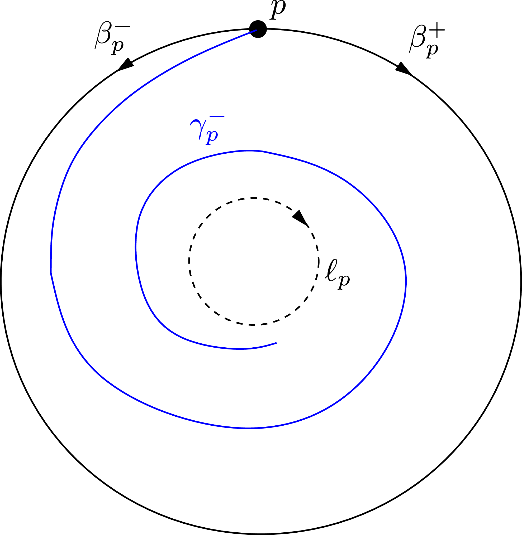
There are four \({\rm Mod}({\Bbb S})-\)invariant oriented bi-infinite geodesics starting at \(p\), see Figure 31, see also paragraph 3 of Section 7 for the key example when \({\Bbb S}\) is an annulus:
The geodesics \(\gamma^-_{p}\) and \(\gamma^+_{p}\) winding in the opposite directions around the neck geodesic \(\ell_p\).
The boundary geodesic with two possible orientations, denoted by \(\beta^-_{p}\) and \(\beta^+_{p}\).
The orientation of \({\Bbb S}\) near \(p\) induces the following order of the oriented geodesics: \(\beta^-_p, \gamma^-_{p}, \gamma^+_{p}, \beta_p^+\).
We denote by \(W^-_p, W^\sharp_p, W^+_p\) are the areas of triangles cut by the horocycle \(h_p\) and the geodesics \((\beta_p^-, \gamma^-_{p}), \;(\gamma^-_{p}, \gamma_p^+), \;(\gamma^+_{p}, \beta_p^+),\) respectively. Clearly one has \[W_p = W^-_p + W^\sharp_p + W^+_p, \quad W_p^-=W_p^+.\] So the reduced potential \(W_p^\sharp\) is given by \[\label{15} W^\sharp_p = W_p - 2W^+_p.\tag{86}\]
The sum of the two terms in the first line of the RHS of (?? ) corresponding to the trouser leg \({\rm T}^\sharp_p\) with two possible orientations of the boundary bi-infinite geodesic \(\beta_p\), which we call the \({\rm T}^\sharp_p-\)term, is given by \[\label{MUF} \int _{{\cal M}_{\Bbb S}({{\rm K}}, {\rm L})}f \;(W^+_p + W_p^-) \; {\Bbb E}_{\Bbb S}.\tag{87}\]
Subtracting (87 ) from the both parts of (?? ), and using (86 ), we get the reduced unfolding formula: \[\label{recur***} \begin{align} &\int _{{\cal M}_{\Bbb S}({{\rm K}}, {\rm L})}f \;W^\sharp_p\; {\Bbb E}_{\Bbb S}\;= \;the RHS of formula (\ref{recur**}) - \{the {\rm T}^\sharp_p-term\}.\\ \end{align}\tag{88}\] Then each integral on the right hand side is the integration over the moduli space for a surface which is simpler than the original one.
6 Tropicalized exponential volumes of moduli spaces↩︎
6.1 Tropicalized moduli spaces and their geometric interpretations↩︎
Recall that a semifield \(\Bbb P\) is a set with the operations of addition, multiplication and division, satisfying the usual axioms. In particular \(\Bbb P\) is an abelian group for the multiplication and division.
The most important example for us is the semifield of positive real numbers \({\mathbb{R}}_{>0}\).
Other important examples are the tropical semifields \({\Bbb A}^t\) associated with the following abelian groups: \[{\Bbb A}= {\mathbb{Z}}, \quad {\Bbb A}={\mathbb{Q}}, \quad {\Bbb A}={\mathbb{R}}.\] The semifield structure is given by \(\alpha \oplus \beta:= {\rm max}(\alpha, \beta), \;\;\alpha\otimes b := \alpha+\beta, \;\;\alpha : \beta := \alpha-\beta.\;\;\)
Since the space \(\mathcal{P}_{\Bbb S}\) has \({\rm Mod}({\Bbb S})-\)equivariant cluster Poisson structure, and since the cluster Poisson transformations are subtraction free, we can consider the set \({\mathcal{P}}_{{\Bbb S}}(\Bbb P)\) of points of the space \({\cal P}_{ {\Bbb S}}\) with values in any semifield \(\Bbb P\), see [3]. Namely, a tropical \(\Bbb P-\)point is defined by assigning to each cluster coordinate system \({\boldsymbol{c}}\) a collection of elements \[(\chi^{\boldsymbol{c}}_1, ..., \chi^{\boldsymbol{c}}_n)\in {\Bbb P}^n, \;\;\;\;\;n = {\rm dim}{\cal P}_{{\Bbb S}},\] related by tropicalized cluster Poisson transformations. For example, positive points of \({\cal P}_{ {\Bbb S}}\) are the points of \({\cal P}_{ {\Bbb S}}\) whose coordinates in one, and hence any, cluster Poisson coordinate system are positive real numbers. The modular group \({\rm Mod}({\Bbb S})\) acts on the set \({\cal P}_{{\Bbb S}}(\Bbb P)\). So we can consider the enhanced moduli orbifold/orbiset \[{\cal M}^{\rm en}_{\Bbb S}(\Bbb P):= {\cal P}_{{\Bbb S}}(\Bbb P)/{\rm Mod}({\Bbb S}).\]
In particular we have sets of positive, and tropical real, rational and integral points of the space \({\cal P}_{\Bbb S}\): \[\label{es} {\cal P}_{\Bbb S}({\mathbb{R}}_{>0}), \quad {\cal P}_{\Bbb S}({\mathbb{R}}^t), \quad {\cal P}_{\Bbb S}({\mathbb{Q}}^t), \quad {\cal P}_{\Bbb S}({\mathbb{Z}}^t).\tag{89}\] Here \({\cal P}_{\Bbb S}({\mathbb{R}}_{>0})\) is a manifold, \({\cal P}_{\Bbb S}({\mathbb{R}}^t)\) is a piecewise linear manifold, and \({\cal P}_{\Bbb S}({\mathbb{Z}}^t)\) is its discrete subset: \[{\cal P}_{\Bbb S}({\mathbb{Z}}^t)\subset {\cal P}_{\Bbb S}({\mathbb{R}}^t).\] Each of the sets (89 ) has a geometric interpretation via the Teichmüller theory [17], see also [24], briefly discussed below.
First, the triple \(({\cal T}^{\rm en}_{\Bbb S}, W, \Omega)\), where \({\cal T}^{\rm en}_{\Bbb S}\) is the enhanced Teichmuller space, has an algebraic geometric avatar: the stack \({\cal P}_{ {\Bbb S}}\) with the \({\rm Mod}({\Bbb S})-\)invariant volume form \(\Omega_{\Bbb S}\), and a regular potential function \({W}= \sum_{p}{W}_p\). Indeed, by Theorem 14, \[{\cal T}^{\rm en}_{\Bbb S}= {\cal P}_{ {\Bbb S}}({\mathbb{R}}_{>0}),\] and the volume form and local potentials on the enhanced Teichmüller space are the restrictions of the form \(\Omega_{\Bbb S}\) and the functions \(W_p\) to the positive locus.
Next, the points of the space \({\cal P}_{ {\Bbb S}}\) with values in the tropical semifields \(\Bbb A^t\), where \(\Bbb A={\mathbb{Z}}, {\mathbb{Q}}, {\mathbb{R}}\), are identified, respectively, with the sets of integral, rational, and real laminations on \({\Bbb S}\). This follows from the description of \({\cal X}-\)laminations on a decorated surface, and coordinates parametrising them, see [24].
6.2 The exponential tropical volumes↩︎
The potential \(W\), the functions \({\rm K}\), and the exponent of the boundary geodesic length \({\rm L}:=e^l\) are Laurent polynomials with positive integral coefficients in any cluster Poisson coordinate system. So they can be tropicalized, providing a \({\rm Mod}({\Bbb S})-\)invariant functions \[W^t, \;{\rm K}^t, \;{\rm L}^t: {\cal P}_{ {\Bbb S}}({\Bbb A}^t)\longrightarrow\Bbb A.\] So we can consider the corresponding spaces of negative laminations \[\label{msms} {\cal M}^-_{\Bbb S}({\Bbb A}^t)(\kappa, \alpha):= \frac{\{\ell\in {\cal P}_{\Bbb S}({\Bbb A}^t)\;| \;{\rm K}^t(\ell) = \kappa, \;\;{\rm L}^t(\ell) = \alpha, \;\;\;W^t(\ell) \leq 0\}}{modulo the action of the group {\rm Mod}({\Bbb S})}.\tag{90}\] The cluster volume form \(\Omega_{\Bbb S}\) induces a volume form \(\Omega_{\Bbb S}^t\) on the space of real tropical points, which provides in each of the tropical cluster Poisson coordinate systems \((\chi_1 \ldots \chi_k)\) the Lebesgue measure \(2\cdot d\chi_1 ... d\chi_k\).
Definition 12. Given a decorated surface \({\Bbb S}\), the exponential tropical volume* is the volume of the real tropical moduli space \({\cal M}^-_{\Bbb S}({\mathbb{R}}^t)(\kappa, \alpha)\) for the tropical volume form \(\Omega^t\): \[\label{def4.1} \begin{align} {\rm Vol}^t_{\cal E}({\cal M}^{\rm en}_{\Bbb S}(\kappa, \alpha)):= &\int_{{\cal M}^-_{{\Bbb S}}({\mathbb{R}}^t)(\kappa, \alpha)}\Omega_{\Bbb S}^t.\\ \end{align}\tag{91}\] *
Remark 27. The tropicalised exponential volume can be obtained by starting with the exponential volume integral, substituting \[{\rm X}_i = e^{\chi_i t}, \;\;{\rm B}_i = e^{\beta_it}, \;\;{\rm K}_i=e^{\kappa_it},\] dividing the integrand by \(t^n\), and then take the limit of the integral when \(t \longrightarrow\infty\). Indeed, the cluster volume form is: \[2\cdot d\log {\rm X}_1 \wedge \ldots \wedge d\log {\rm X}_n = 2\cdot t^n d\chi_1\wedge \ldots \wedge d\chi_n.\] This is why we divide the integral by \(t^n\) before taking the limit.
Theorem 28. For any decorated surface \({\Bbb S}\), the exponential tropical volume (91 ) is finite: \[{\rm Vol}^t_{\cal E}({\cal M}^{\rm en}_{\Bbb S}(\kappa, \alpha))<\infty.\]
When \({\Bbb S}=S\) is a surface with punctures but without the special boundary points this follows from Theorem 30 below. The general case reduces to this, see Section 6.4.
6.3 Tropical volumes of moduli spaces for punctured surfaces = Kontsevich volumes↩︎
In Section 6.3 let \({\Bbb S}:=S\) be a connected genus \(g\) surface with \(n\) punctures but without boundary points.
In his proof of Witten’s Conjecture, M. Konstevich [25] introduced a combinatorial model \({\cal M}^{\rm comb}_{g,n}\) of the moduli space \({\cal M}_{g,n}\). It is an orbifold, parametrising equivalence classes of metrised connected ribbon graphs \(\Gamma\), that is ribbon graphs with vertices of valency \(\geq 3\) and positive real numbers at the edges, so that the associated oriented surface has genus \(g\) and \(n\) holes. By [25], there is a homeomorphism \[\zeta: {\cal M}_{g,n}\times {\mathbb{R}}_+^n \stackrel{\sim}{\longrightarrow} {\cal M}^{\rm comb}_{g,n}.\] It assignes to a surface \(S\) and a collection of positive numbers \(\alpha=\{\alpha_1, ..., \alpha_n\}\) the Jenkins-Strebel differential with the critical graph \(\Gamma\), whose perimeters of boundary components are given by the set \({\rm L}\). See also [4].
The space \({\cal M}^{\rm comb}_{g,n}\) has a Poisson structure \(\{*,*\}_{\rm K}\) given by the bivector \[\label{PSK} \beta_{\rm K}= \sum_{e} \frac{\partial}{\partial \alpha_e}\wedge \frac{\partial}{\partial \alpha_{s(e)}}.\tag{92}\] Here the sum is over all oriented edges \(e\) of the graph \(\Gamma\), \(\alpha_e>0\) is the number assigned to the edge, and \(s\) is the cyclic clockwise for the ribbon structure of \(\Gamma\) shift by one, acting on the set of oriented edges sharing the same initial vertex.
The subspace of metrised graphs with a given set of perimeters \(\alpha\) is denoted by \({\cal M}^{\rm comb}_{g,n}(\alpha)\). They are the symplectic leaves for the Poisson structure. Their volumes are defined by \[\label{118a} {\rm Vol}({\cal M}^{\rm comb}_{g,n}(\alpha)):= \int_{{\cal M}^{\rm comb}_{g,n}(\alpha)}e^{8\beta_{\rm K}^{-1}}.\tag{93}\] Here \(\beta_{\rm K}^{-1}\) is the symplectic form induced by the Poisson bivector \(\beta_{\rm K}\) restricted to the fibers. The coefficient \(8\) comes from [26].
Note that since the surface \(S\) has no boundary points \({\cal P}_S={\cal X}_S\). By [17], for each puncture of \(S\) the group \({\mathbb{Z}}/2{\mathbb{Z}}\) acts by positive birational transformations of the moduli space \(\mathcal{X}_S\). The set \(\mathcal{X}_S({\mathbb{R}}^t)\) of real tropical points of the space \(\mathcal{X}_S\) parametrises measured \({\cal X}-\)laminations on \(S\) [17]. So the group \({\mathbb{Z}}/2{\mathbb{Z}}\) acts on the space \(\mathcal{X}_S({\mathbb{R}}^t)\) by the tropicalization. So the group \({\rm Mod}(S) \times ({\mathbb{Z}}/2{\mathbb{Z}})^n\) acts on the space of \(\mathcal{X}_S({\mathbb{R}}^t)\).
Let us expand the punctures to holes. Consider the set \({\cal C}_S\) of pairs (an ideal triangulation of \(S\), a choice of boundary orientations of all holes on \(S\)). The group \({\rm Mod}(S) \times ({\mathbb{Z}}/2{\mathbb{Z}})^n\) acts on the set \({\cal C}_S\). The set \({\cal C}_S\) parametrises coordinate systems on \(\mathcal{X}_S({\mathbb{R}}^t)\), called ideal coordinate systems. So for each ideal triangulation \({\cal T}\) of \(S\) there are \(2^n\) ideal coordinate systems.
There are two flavors of moduli spaces related to \(S\): the classical one, and its enhanced variant:12 \[\begin{align} &{\cal M}_S = {\cal M}_S({\mathbb{R}}_{>0}) \;:= {\cal T}^{\rm en}_S/({\rm Mod}(S)\times ({\mathbb{Z}}/2{\mathbb{Z}})^n), \\ &{\cal M}^{\rm en}_S = {\cal M}^{\rm en}_S({\mathbb{R}}_{>0}):= {\cal T}^{\rm en}_S/{\rm Mod}(S). \\ \end{align}\] The moduli space \({\cal M}^{\rm en}_S\) is a \(2^n:1\) ramified cover of the classical one \({\cal M}_S\). Specifying the lengths \({\rm L}=(l_1, ..., l_n)\) of boundary geodesics, we get the fibers \({\cal M}_S({\rm L})\) and \({\cal M}^{\rm en}_S({\rm L})\). When \({\rm L}=0\), we have \[{\cal M}_S(0) = {\cal M}^{\rm en}_S(0) = {\cal M}_{g,n}.\]
If \(\alpha_1...\alpha_n\not = 0\), the tropical moduli space \({\cal M}^{\rm en}_S({\mathbb{R}}^t)(\alpha)\) has \(2^n\) components. They are permuted by the \(({\mathbb{Z}}/2{\mathbb{Z}})^n-\)action, altering the signs of \((\alpha_1, ..., \alpha_n)\). The classical component is the one with \(\alpha_1, ..., \alpha_n\geq 0\).
Let \(d=3g-3+n\), so that \(2d\) is the dimension of the symplectic fiber. In particular, \(d = {\rm dim}{\cal M}_{g,n}\).
The volume form \(\Omega^t_S(\alpha)\) induced on the symplectic fibers \({\cal M}^{\rm en}_S({\mathbb{R}}^t)(\alpha)\) by the tropical cluster volume form \(\Omega^t_S = 2\cdot d\chi_{{\rm E}_1} \wedge ... \wedge d\chi_{{\rm E}_n}\) is a multiple of the tropical volume form on the symplectic fibers: \[\frac{(8\beta_{\rm K}^{-1})^d}{d!}= {\sigma}_S \cdot \Omega^t_S(\alpha).\] By [25] and [26], the constant \(\sigma_S\) is given by13 \[\sigma_S:=\frac{\prod dp_i \cdot \frac{(8 \beta_{\rm K}^{-1})^{3g-3+n}}{(3g-3+n)!}}{2\cdot \prod_{{\rm E}} |d \chi_{{\rm E}}|}\; = 2^{5g-6+2n} = 4^d\cdot 2^{-g}.\] The parameters \(p_i\) are perimeters of the metrised ribbon graphs.
Adapting definition (91 ) for the moduli space \({\cal M}_S({\mathbb{R}}^t)(\alpha)\), we have \[\label{def4.1a} \begin{align} {\rm Vol}^t({\cal M}_S({\mathbb{R}}^t)(\alpha)):= &\int_{{\cal M}_{S}({\mathbb{R}}^t)(\alpha)}\Omega_S^t(\alpha).\\ \end{align}\tag{94}\] Similar formula holds for the tropical space \({\cal M}^{\rm en}_S({\mathbb{R}}^t)(\alpha)\).
Theorem 29. Let \(S\) be a connected genus \(g\) oriented topological surface with \(n\) punctures. Then the volume of the orbispace \({\cal M}^{\rm comb}_{g,n}(\alpha)\) in (93 ) relates to the tropical volume of the space \({\cal M}_S({\mathbb{R}}^t)(\alpha)\) by: \[\label{85} \begin{align} {\rm Vol}({\cal M}^{\rm comb}_{g,n}(\alpha)) = & \sigma_S\cdot {\rm Vol}^t({\cal M}_S({\mathbb{R}}^t)(\alpha))\\ =& \sigma_S\cdot{\rm Vol}^t({\cal M}^{\rm en}_S({\mathbb{R}}^t)(\alpha)).\\ \end{align}\qquad{(31)}\]
Proof. The tropicalization of the cluster Poisson coordinates \(\{X_{\rm E}\}\) on the space \({\cal X}_S\) delivers the cluster Poisson coordinates \(\{\chi_{\rm E}\}\) on the real tropical space \(\mathcal{X}_S({\mathbb{R}}^t)\) [17]. It follows from Theorem 9 that the induced cluster Poisson bracket on the space \(\mathcal{X}_S({\mathbb{R}}^t)\) is given by \[\label{PSFG} \{\chi_{\rm E}, \chi_{\rm F}\}_{\rm cl} = \varepsilon_{{\rm E}{\rm F}}.\tag{95}\]
An \({\cal X}-\)lamination \(\ell\) on \(S\) is called positive, if there exists an ideal coordinate system on \(S\) such that the coordinates \(\chi_{\rm E}(\ell)\) of \(\ell\), assigned to the edges \({\rm E}\) of the underlying ideal triangulation, are positive: \(\chi_{\rm E}(\ell)>0\). By [17] there is a dense open subset of positive \({\cal X}-\)laminations. For any positive \({\cal X}-\)lamination such an ideal coordinate system is unique. The complement to the set of positive laminations has measure zero.
There is a bijection between ideal triangulations \({\cal T}\) of \(S\) and trivalent ribbon graphs \(\Gamma\) of genus \(g\) with \(n\) holes. It assigns to an ideal triangulation \({\cal T}\) its dual graph \(\Gamma_{\cal T}\). The orbits of ideal triangulations of \(S\) under the action of the group \({\rm Mod}(S)\) correspond to the isomorphism classes of trivalent ribbon graphs.
Trivalent metrised ribbon graphs form an open dense subset of full measure of \({\cal M}^{\rm comb}_{g,n}\). The correspondence between ideal triangulations of \(S\) and ribbon graphs of type \((g,n)\) extends to an isomorphism \[\label{IDI} \begin{align} &The open dense part {\cal M}^{\times}_S({\mathbb{R}}^t)\subset \mathcal{M}_S({\mathbb{R}}^t), parametrising positive {\cal X}-laminations \stackrel{\sim}{\longrightarrow} \\ &The open dense part {\cal M}^{\times, {\rm comb}}_{g,n}\subset {\cal M}^{\rm comb}_{g,n}, parametrising (metrised trivalent ribbon graphs)/{\rm Iso}.\\ \end{align}\tag{96}\] For an ideal triangulation \({\cal T}\) of \(S\), it assigns to a positive lamination \(\ell\) with the coordinates \(\chi_{\rm E}(\ell)>0\) the trivalent ribbon graph \(\Gamma_{\cal T}\) metrised by the numbers \(\chi_{\rm E}(\ell)\) at the edges \({\rm E}\).
Lemma 14. Isomorphism (96 ) provides a Poisson isomorphism \[\label{PKISO} ({\cal M}^{\times}_S({\mathbb{R}}^t), \{*,*\}_{\rm cl}) \longrightarrow({\cal M}^{\times, {\rm comb}}_{g,n}, \{*,*\}_{\rm K}).\qquad{(32)}\]
The isomorphism (?? ) identifies the perimeters \(p_i\) of metrised ribbon graphs with the values of tropical Casimir functions. This and Lemma 14 imply formula (?? ). ◻
By Kontsevich’s theorem [26], [25] we have, where \(d = {\rm dim}{\cal M}_{g,n}=3g-3+n\): \[\begin{align} {\rm Vol}({\cal M}^{\rm comb}_{g,n}(\alpha)) = & \sum_{d_1+ ...+d_n =d} \frac{\alpha_1^{2d_1}}{d_1!} \ldots \frac{\alpha_n^{2d_n}}{d_n!} \int_{\overline{\cal M}_{g,n}}\psi_1^{d_1}\cdots \psi_n^{d_n}\\ =& \frac{1}{d!} \;\int_{\overline{\cal M}_{g,n}}(\alpha_1^2\psi_1 + \ldots + \alpha_n^2\psi_n)^{d} .\\ \end{align}\] We recall that Kontsevich [26] defines the volume using the form \({\rm exp}(8\beta_{\rm K}^{-1})\), see (93 ).
This and Theorem 29 immediately imply
Theorem 30. Tropical volumes of moduli spaces \({\cal M}_S({\mathbb{R}}^t)(\alpha)\) of \(\mathcal{X}-\)laminations on a genus \(g\) surface with \(n\) punctures \(S\) carry the same information as the intersection theory on \(\overline{\cal M}_{g,n}\). Precisely, \[\label{TRV} \begin{align} \int_{\overline{\cal M}_{g,n}}e^{\alpha_1^2\psi_1 + \ldots + \alpha_n^2\psi_n} = \frac{1}{d!}\;\int_{\overline{\cal M}_{g,n}}(\alpha_1^2\psi_1 + \ldots + \alpha_n^2\psi_n)^{d} = &\sigma_S\cdot{\rm Vol}^t({\cal M}_S({\mathbb{R}}^t)(\alpha))\\ =& \sigma_S \cdot {\rm Vol}^t({\cal M}^{\rm en}_S({\mathbb{R}}^t)(\alpha)).\\ \end{align}\qquad{(33)}\]
Let us now compare the top degree \(d\) part \({\rm Vol}_{\rm top}(\mathcal{M}_S({\rm L}))\) of the volume polynomial \({\rm Vol}_{\rm WP}(\mathcal{M}_S({\rm L}))\) for the Weil-Peterssen volume form, and the tropical volume \({\rm Vol}^t({\cal M}_S({\mathbb{R}}^t)(\alpha))\). Mirzakhani calculated the volume polynomial \({\rm Vol}_{\rm WP}(\mathcal{M}_S({\rm L}))\). Therefore by [13] and [5], see (8 ) we get the formula for the top degree part of the Weil-Peterssen volume polynomial: \[\label{V1z} \begin{align} {\rm Vol}_{\rm top}(\mathcal{M}_S({\rm L})) = &\sum_{d_1+\ldots + d_n = d} {\cal V}_{g, d_1, ..., d_n}\cdot l_1^{2d_1} \ldots l_n^{2d_n};\\ & {\cal V}_{g, d_1, ..., d_n} \stackrel{(\ref{WCM})}{=} \frac{1}{2^dd!}\cdot \int_{\overline{\cal M}_{g,n}}\psi_1^{d_1}\cdots \psi_n^{d_n}.\\\end{align}\tag{97}\] It is handy to introduce the following notation: \[\label{10.24.24} {\cal V}^*_{g, d_1, ..., d_n} \stackrel{}{=} \frac{2^dd!}{d_1!...d_n!}{\cal V}_{g, d_1, ..., d_n}.\tag{98}\]
Remark 31. Mirzakhani’s \({\rm L}=(l_1, ..., l_n)\) are the lengths of boundary geodesics on hyperbolic surfaces homeomorphic to \(S\). Our \(\alpha=(\alpha_1, ..., \alpha_n)\) have different nature: they are parameters on measured laminations on \(S\). We relate them using Kontsevich’s perimeter parameters. Namely, we relate the real tropical space of measured laminations with Kontsevich’s combinatorial moduli space, identifying \(\alpha\)’s with Kontsevich’s perimeter parameters, also denoted by \(\alpha = (\alpha_1, ..., \alpha_n)\). Then we match the two sets: \[{\rm L}=(l_1, ..., l_n) \longleftrightarrow \alpha = (\alpha_1, ..., \alpha_n).\] Note that in Section 6 we used systematically the small greek letters for the tropical parameters, reserving the latin letters for the geometric one. Here we match the two, in a somewhat mysterious way.
Keeping this remark in mind, and combining (98 ) with (97 ) and formula (?? ) for the tropical volume polynomial, we get: \[\label{V1za} \begin{align} {\rm Vol}^t(\mathcal{M}_S({\mathbb{R}}^t)(\alpha)) = & \sigma_S^{-1} \sum_{d_1+\ldots + d_n = d} \int_{\overline{\cal M}_{g,n}}\frac{(\alpha_1^2\psi_1)^{d_1}\cdots (\alpha^2_n\psi_n)^{d_n} }{d_1! \ldots d_n!}\\ \stackrel{( \ref{V1z})}{=}& \sigma_S^{-1} \sum_{d_1+\ldots + d_n = d} {\cal V}^*_{g, d_1, ..., d_n}\cdot \alpha_1^{2d_1} \ldots \alpha_n^{2d_n}.\\ \end{align}\tag{99}\]
6.4 Calculating tropicalised exponential volumes↩︎
If \({\Bbb S}={\rm D}_n^*\) is a punctured disc with \(n\) marked points, the Teichmuller space coincides with the moduli space. The tropical moduli space \({\cal M}_{{{\rm D}_n^*}}({\mathbb{R}}^t)( {\kappa}, \alpha)\) carries real functions \(\chi_i, \beta_i, \kappa_i\), \(i \in {\mathbb{Z}}/n{\mathbb{Z}}\). We consider the variables \(\kappa= (\kappa_1, \ldots \kappa_n)\) as fixed parameters, so the fiberwise tropical cluster volume form is \[\Omega^t_{\Bbb S}(\kappa) :=2d\log \beta_1 \wedge \ldots \wedge d\log \beta_{n}.\]
Lemma 15. a) The tropicalization of the exponential volume of the moduli space for \({\Bbb S}={\rm D}_n^*\) is given by \[{\rm{Vol}}^t_{\mathcal{E}}({\rm D}_{n}^*)({\kappa}) = 2\prod_{i=1}^n \kappa_i.\]
b) For any integer \(d \geq 0\), the following integral is a polynomial in \(\kappa= (\kappa_1, ..., \kappa_{n-1})\). \[\int_0^\infty {\rm{Vol}}^t_{\mathcal{E}}({\rm D}_{n}^*)({\kappa},\alpha)\; \alpha^{d} d \alpha.\]
Proof. a) The tropicalized potential \(W^t\) provides inequalities: \[W^t= {\rm max}\Bigl(\beta_1, \kappa_1 - \beta_1, \ldots \beta_n, \kappa_n-\beta_n\Bigr)\leq 0 \;\;\;\;\longleftrightarrow \;\; \;\;\kappa_i \leq \beta_i \leq 0, \;\;\forall i \in {\mathbb{Z}}/n{\mathbb{Z}}.\]
b) The tropicalization of integral (70 ) delivers system of inequalities \[\begin{align} &\kappa_{i} \leq \beta_{i} \leq 0, \;\; \;\;\;i=1, ..., n-1,\\ &\kappa_n + \sum_{i=1}^{n-1}\kappa_{i} \leq \alpha+2\sum_{i=1}^{n-1} \beta_i \leq - \kappa_n + \sum_{i=1}^{n-1}\kappa_i. \\ \end{align}\] So given \(\kappa\), this determines a finite polyhedron in the space \({\mathbb{R}}^n\) with the coordinates \((\beta_1, ..., \beta_{n-1}, \alpha)\). ◻
Proposition 32. For any decorated surface \({\Bbb S}\) we have the tropical neck recursion formula:14 \[\label{MFOa} {\rm Vol}^t_{\cal E}({\cal M}_{{\Bbb S}}({\kappa}, \alpha)) = {\rm C}_{\Bbb S}\sum_{d_1+ ... + d_m= 3g-3+m} {\cal V}^*_{g, d_1, ..., d_m} \prod_{j=1}^r \int^\infty_{0} {\rm{Vol}}^t_{\mathcal{E}}({\rm D}_{n_j}^*)({\kappa}_j, \alpha_j)\; \alpha_j^{2d_j+1} d \alpha_j.\qquad{(34)}\]
Proof. Let \({\Bbb S}_\ell:= {\Bbb S}-{\rm C}_\ell\) be the decorated surface obtained by cutting out from \({\Bbb S}\) the crown \({\rm C}_\ell\) with the neck loop \(\ell\). Denote by \(r\) the number of cusps on the crown \({\rm C}_\ell\). There is the real tropical analog of the Fenchel–Nielsen coordinates, see [27] for the classical formulation, adopted to our setting as follows: there is an isomorphism: \[{\cal P}_{\Bbb S}({\mathbb{R}}^t) \stackrel{\sim}{=} {\cal P}_{{\Bbb S}_\ell}({\mathbb{R}}^t)\times {\mathbb{R}}^2\times {\cal P}_{{\rm D}^*_r}({\mathbb{R}}^t).\] Here the first coordinate in \({\mathbb{R}}^2\) is given by the intersection number of the measured lamination \(\mu\) with the loop \(\ell\), that is the total measure of the loop for the transverse measure \(\mu\). We use it, together with the fact that \({\rm Mod}({\Bbb S})= {\rm Mod}({\Bbb S}_\ell)\times \mathbb{Z}\), similarly to the classical case, except that we use the tropical volume form. ◻
6.4.0.1 Proof of Theorem 28.
It follows from Lemma 15, Proposition 32, and Theorem 30.
7 Examples↩︎
7.1 The annulus \({\rm A}_{1,1}\) with a cusp on each boundary component↩︎
Recall the coordinates \({\rm K}_{a}, {\rm K}_{b}, {\rm K}_{p}\) at the sides opposite to the vertices \((a,b,p)\) of the geodesic triangle \(\tau\) on Figure 26. The potential of the triangle \(\tau\) is given by \[\label{EXVt} \begin{align} {W}_{\tau}({\rm K}_a, {\rm K}_b, {\rm K}_p) =& \Bigl(\frac{{\rm K}_{p}}{{\rm K}_{a}{\rm K}_{b}}\Bigr)^{-\frac{1}{2}} + \Bigl(\frac{{\rm K}_{a}}{{\rm K}_{p}{\rm K}_{b}}\Bigr)^{-\frac{1}{2} }+\Bigl(\frac{{\rm K}_{b}}{{\rm K}_{a}{\rm K}_{p}}\Bigr)^{-\frac{1}{2}}.\\ \end{align}\tag{100}\]
7.1.1 The annulus \({\rm A}_{p,q}\) and \({\rm Mod}({\rm A}_{p,q})\).↩︎
Denote by \({\rm A}_{p,q}\) the annulus with \(p\) marked points on one of the components, and \(q\) on the other. There is a unique neck geodesic loop \(\ell\). Its length is denoted by \(l\). The pure mapping class group \({\rm Mod}({\rm A}_{p,q})\) is generated by the Dehn twist \({\rm D}_\ell\) around \(\ell\). It is trivial if one of the integers \(m,n\) is zero, and is isomorphic to \({\mathbb{Z}}\) otherwise: \[\begin{align} &{\rm Mod}({\rm A}_{p,q})={\mathbb{Z}}, \qquad p,q\not =0. \\ & {\rm Mod}({\rm A}_{0,q})={\rm Mod}({\rm A}_{p,0})= 0. \\ \end{align}\] If the mapping class group is trivial, the Teichmüller space is the same as the moduli space.
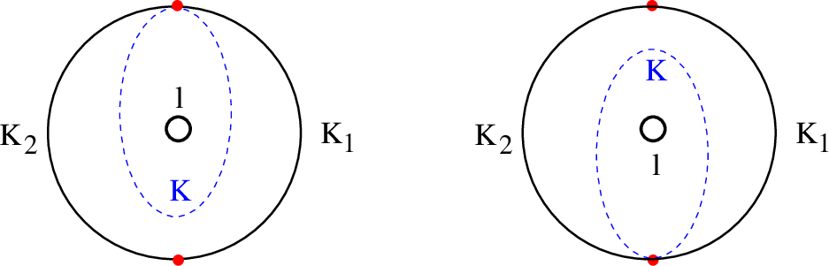
Calculation of the exponential volume for the annulus \({\rm A}_{p,q}\) reduces to the case when \(p,q \leq 1\). Namely, if, for example, \(p\geq 2\), we cut out an ideal \((p+1)-\)gon which has \(p\) boundary sides, and one side given by the bi-infinite geodesic \(\gamma\) at a cusp, surrounding the other boundary component. This way we get the decorated surface \({\rm A}_{1,q}\), which we can reduce to \({\rm A}_{1,1}\) by cutting out an ideal \((q+1)-\)gon. Let us elaborate first this step in the simplest case, and then concentrate in the most interesting case of the annulus \({\rm A}_{1,1}\).
7.1.2 The annulus \({\rm A}_{0,2}\).↩︎
The cluster Poisson coordinates on the Teichmüller space of \({\rm A}_{0,2}\) are \(\{{\rm K}_1, {\rm K}_2, {\rm B}, {\rm X}\}\). We have \({\rm X}= {\rm L}=e^{l}\). Using (100 ) and (75 ), we get the following integral for its volume, see Figure 32: \[\label{5555} \begin{align} & {\rm Vol}_{\cal E}({\cal M}_{{\rm A}_{0,2}})({\rm K}_1, {\rm K}_2; {\rm L}) =\\ & \int_{0}^\infty {\rm exp}\Bigl( -W_\tau({\rm K}_1, {\rm K}_2, {\rm K}) - {\rm K}^{\frac{1}{2}}({\rm L}^{\frac{1}{2}}+ {\rm L}^{-\frac{1}{2}})\Bigr) d\log {\rm K}.\\ \end{align}\tag{101}\] Starting at the other cusp we get the same integrand. The two are related by a sequence of two flips.
7.1.3 The McShane identity for the annulus \({\rm A}_{1,1}\).↩︎
There is a collection of bi-infinite geodesics \(\{\gamma_n\}\), \(n \in {\mathbb{Z}}\), connecting the two cusps \(p\) and \(q\). They represent all isotopy classes of arcs connecting the two cusps, and form a principal homogeneous set for the action of \({\rm Mod}({\rm A}_{1,1})\), so that \({\rm D}_l(\gamma_n) = \gamma_{n+1}\). In the limit when \(n \to \pm \infty\), we get bi-infinite geodesics \(\gamma_p^-\) and \(\gamma_p^{+}\) starting at \(p\) and winding around the geodesic \(\ell\). There is a unique bi-infinite boundary geodesic \(\beta_p\) from the cusp \(p\) to itself.
Moving the end of the geodesic \(\gamma_n\) along the boundary geodesic \(\beta_q\) till we get the geodesic \(\gamma_{n+1}\), we fill the ideal geodesic triangle \(\tau_{p, n}\). Denote by \(h_p\) the horoarc at the cusp \(p\), and by \(h_{{\tau}_n}\) its intersection with the triangle \(\tau_{p,n}\). Denote by \(d_{p, \pm}\) the arcs on the horocycle \(h_p\) between \(\beta_p\) and \(\gamma_{\pm\infty}\). Then we have \[length(h_p) = length(d_{p, -}) + \sum_{n \in {\mathbb{Z}}} length(h_{{\tau}_n}) + length(d_{p, +}).\] This is the McShane identity for the cusp \(p\). It can be rewritten via potentials as follows. Let \(W_p\) be the potential at \(p\), and by \(W_{p,n}\) the potential at \(p\) of the geodesic triangle \(\tau_{p, n} = (\gamma_n, \gamma_{n+1}, \beta_q)\). Then we get: \[\begin{align} &W_p = 2 {\rm K}_p^{\frac{1}{2}}{\rm L}^{-\frac{1}{2}} + \sum_{n \in {\mathbb{Z}}} W_{p,n}.\\ &W_p^\sharp = \sum_{n \in {\mathbb{Z}}} W_{p,n}.\\ \end{align}\]
7.1.4 Annulus \({\rm A}_{1,1}\).↩︎
There are two ways to calculate the exponential volume: using the neck recursion formula, and using unfolding formula (?? ). Let us elaborate each of them.
1. Denote by \({\rm K}_1, {\rm K}_2\) the frozen coordinates at the boundary circles, see Figure 33, and by \({\rm X}, {\rm Y}\) the cluster Poisson coordinates for the geodesics \(\gamma_x, \gamma_y\) (which were denoted by \(\gamma_0, \gamma_1\) above) of the triangulation given by these two geodesics and boundary arcs, shown on the right on Figure 33.
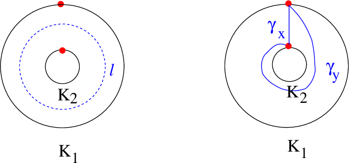
One has \[\{{\rm X}, {\rm Y}\} = -2 {\rm X}{\rm Y}.\] The other Poisson brackets are \[\{{\rm B}_1, {\rm X}\} = -{\rm B}_1{\rm X}, \;\;\;\{{\rm B}_1, {\rm Y}\} = {\rm B}_2{\rm Y}, \;\;\;\{{\rm B}_2, {\rm X}\} = -{\rm B}_2{\rm X},\;\;\;\{{\rm B}_2, {\rm Y}\} = {\rm B}_2{\rm Y}, \;\;\;\{{\rm B}_1, {\rm B}_2\}=0.\] The following elements \({\rm K}_1, {\rm K}_2\) are in the center of the Poisson bracket \(\{*,*\}\): \[\label{K1K2} {\rm K}_i = {\rm B}_i^2{\rm X}{\rm Y}, \;\;\;i =1,2.\tag{102}\] The Dehn twist acts by the cluster Poisson transformation given by the flip at \(\gamma_y\) followed by the symmetry \(({\rm X},{\rm Y}) \longmapsto({\rm Y},{\rm X})\). It preserves the frozen variables \({\rm K}_1, {\rm K}_2\).
Then the exponential volume is given by15 \[\label{101a} \begin{align} {\rm Vol}_{\cal E}({\cal M}_{{\rm A}_{1,1}})({\rm K}_1, {\rm K}_2) = \frac{1}{2} \; &\int_{{\cal M}_{{\rm A}_{1,1}}}e^{-({\rm B}_1+{\rm B}_2)(1+{\rm X}+{\rm X}{\rm Y})} d\log {\rm X}\wedge d\log {\rm Y}. \\ = \frac{1}{2} \;& \int_{{\cal M}_{{\rm A}_{1,1}}}{\rm exp}\Bigl({-({\rm K}_1^{\frac{1}{2}}+{\rm K}_2^{\frac{1}{2}})({\rm X}{\rm Y})^{-\frac{1}{2}}(1+{\rm X}+{\rm X}{\rm Y})} \Bigr) d\log {\rm X}\wedge d\log {\rm Y}.\\ \end{align}\tag{103}\] To calculate this integral we have to pick a fundamental domain for the Dehn twist. For the annulus \({\rm A}_{1,1}\) this is easy using the Fenchel–Nielsen coordinates, and leads to the neck recursion formula \[\label{100} {\rm Vol}_{\cal E}({\cal M}_{{\rm A}_{1,1}})({\rm K}_1, {\rm K}_2) = \frac{1}{2} \int^\infty_{1} {\rm exp}\Bigl(-({\rm K}_1^{\frac{1}{2}} + {\rm K}_2^{\frac{1}{2}} )({\rm L}^{\frac{1}{2}}+ {\rm L}^{-\frac{1}{2}}) \Bigr) \log {\rm L}\;d \log {\rm L}.\tag{104}\] If the limits of the integration were \((0, \infty)\), this will be the derivative at \(s=0\) of the Bessel function. However the limits are \((1, \infty)\), and this integral can not be reduced to the Bessel integral.
Lemma 16. The variable \({\rm L}^{\frac{1}{2}}\) is related to the variables \(({\rm X},{\rm Y})\) by the equation \[\label{tt1} ({\rm X}{\rm Y})^{-\frac{1}{2}}(1+{\rm X}+{\rm X}{\rm Y}) = {\rm L}^{\frac{1}{2}} +{\rm L}^{-\frac{1}{2}}.\qquad{(35)}\]
Proof. The potential \(W_1\) at the cusp at the crown supporting the coordinate \({\rm K}_1\) can be calculated in two ways: by cutting \({\rm A}_{1,1}\) along the neck geodesic \(\ell\) of the length \(l\), as shown on the left of Figure 33, or by formula (?? ) applied to the triangulated annulus \({\rm A}_{1,1}\) on the right of Figure 33. So we get \[\label{103} \begin{align} & W_1={\rm K}_1^{\frac{1}{2}}({\rm L}^{\frac{1}{2}}+{\rm L}^{-\frac{1}{2}}).\\ &W_1= {\rm B}_1(1+{\rm X}+{\rm X}{\rm Y}). \\ \end{align}\tag{105}\] Using (102 ), and comparing the two equations (105 ) we get the formula. ◻
This is, of course, equivalent to relating the integrands in (103 ) and (104 ).
2. For the fourth term of unfolding formula (?? ) we use the \({\rm K}-\)coordinates for the triangle sides, denoted by \({\rm A},{\rm B}, {\rm K}_1, {\rm K}_2\). We denote by \({\rm X},{\rm Y}\) the cluster Poisson coordinates, so that the coordinates \({\rm A}, {\rm X}\) are assigned to the edge \(\gamma_x\), and \({\rm B}, {\rm Y}\) to \(\gamma_y\) on Figure 33. Then we have: \[\label{tt}
{\rm X}= \frac{({\rm K}_1{\rm K}_2)^{\frac{1}{2}}}{{\rm B}}, \quad {\rm Y}= \frac{{\rm A}}{({\rm K}_1{\rm K}_2)^{\frac{1}{2}}}.\tag{106}\] Then using the unfolding formula (?? ) for \(f=1/W_p^\sharp\), and
formula (100 ) for the potential \(W_\tau\), we get16 \[\label{101}
\begin{align}
& {\rm Vol}_{\cal E}({\cal M}_{{\rm A}_{1,1}})({\rm K}_1, {\rm K}_2) \\
&= \int_0^\infty\int_0^\infty \left(\frac{{\rm A}{\rm B}}{{\rm K}_1{\rm K}_2}\right)^{\frac{1}{2}}\;\frac{ {\rm exp}\Bigl(- W_\tau({\rm A},{\rm B},{\rm K}_1) - W_\tau({\rm A},{\rm B},{\rm K}_2)\Bigr)}{ ({\rm L}^{\frac{1}{2}} - {\rm L}^{-{\frac{1}{2}}
})} d \log {\rm A}\wedge d \log {\rm B}.\\
\end{align}\tag{107}\]
3. Let us check unfolding formula (?? ) for the function \(f=1\) at the cusp \(p\). We start with \[\int_{{\cal M}_{{\rm A}_{1,1}}}W^\sharp_pe^{-W}\Omega.\] Cutting along the geodesic loop \(\alpha\) and using the neck recursion formula, and using (75 ) twice, we get \[\label{555} \begin{align} & \int_{{\cal M}_{{\rm A}_{1,1}}}W^\sharp_pe^{-W}\Omega = \int^\infty_{0} W^\sharp_pe^{-W_p-W_q} ldl \\ &= \int^\infty_{0} {\rm K}_1^{\frac{1}{2}}(e^{l/2}- e^{-l/2} ) {\rm exp}\Bigl(-({\rm K}_1^{\frac{1}{2}} + {\rm K}_2^{\frac{1}{2}} )(e^{l/2}+ e^{-l/2}) \Bigr) l d l.\\ \end{align}\tag{108}\] This integral is calculated via the Bessel function as follows. Observe that \[-\frac{d}{dl} \;{\rm exp}(-{\rm K}(e^{l/2}+ e^{-l/2})) = \frac{1}{2}{\rm K}(e^{l/2}- e^{-l/2} ) {\rm exp}(-{\rm K}(e^{l/2}+ e^{-l/2})).\] So integrating by parts, and observing that \(l {\rm exp}(-{\rm K}(e^{l/2}+ e^{-l/2}))\) vanishes at \(l=\infty, 0\), we get \[\label{UFF1} \begin{align} & \frac{ 2{\rm K}_1^{\frac{1}{2}}}{{\rm K}_1^{\frac{1}{2}} + {\rm K}_2^{\frac{1}{2}} } \int^\infty_{0} {\rm exp}\Bigl(-({\rm K}_1^{\frac{1}{2}} + {\rm K}_2^{\frac{1}{2}} )(e^{\frac{l}{2}}+ e^{-\frac{l}{2}}) \Bigr) d l \\ &= \frac{2{\rm K}_1^{\frac{1}{2}}}{{\rm K}_1^{\frac{1}{2}} + {\rm K}_2^{\frac{1}{2}} } \int^\infty_{-\infty} {\rm exp}\Bigl(-({\rm K}_1^{\frac{1}{2}} + {\rm K}_2^{\frac{1}{2}} )(e^{l}+ e^{-l}) \Bigr) d l. \\\end{align}\tag{109}\] Note that the integrand in the first line, denoted \({\rm I}(l)\), is an even function of \(l\). So \(\int_{0}^\infty {\rm I}(l) dl = \frac{1}{2}\int_{-\infty}^\infty {\rm I}(l) dl\). Then we change variables \(l/2\to l\).
On the other hand, cutting out the triangle with the sides supporting the variables \({\rm A},{\rm B}, {\rm K}_2\), and using formula (?? ) for the function \(f=1\), we get \[{\rm K}^{-{\frac{1}{2}}}_2\int ({\rm A}{\rm B})^{{\frac{1}{2}}}
{\rm exp}\Bigl(- W_\tau({\rm A},{\rm B},{\rm K}_1) - W_\tau({\rm A},{\rm B},{\rm K}_2)\Bigr)\frac{d{\rm A}}{{\rm A}} \wedge \frac{d{\rm B}}{{\rm B}}.\] Changing the variables \({\rm P}:= ({\rm A}/{\rm B})^{1/2}\),
\({\rm Q}:=({\rm A}{\rm B})^{1/2}\) we get the same result as in (109 ): \[2 {\rm K}^{-{\frac{1}{2}}}_2\int_0^\infty {\rm exp}\Bigl(-({\rm K}_1^{{\frac{1}{2}}} +{\rm
K}_2^{{\frac{1}{2}}} )({\rm P}+{\rm P}^{-1} ) \Bigr)d\log {\rm P}\cdot \int_0^\infty {\rm exp}\Bigl( - ({\rm K}^{-{\frac{1}{2}}} _1+{\rm K}^{-{\frac{1}{2}}} _2){\rm Q}\Bigr)\; \; d {\rm Q} = (\ref{UFF1}).\] Indeed, set \({\rm P}=e^l\). This confirms unfolding formula (?? ).
Problem. Check directly that (104 ) = (107 ): \[\label{99} \begin{align} &2 \int_0^\infty\int_0^\infty \left(\frac{{\rm A}{\rm B}}{{\rm K}_1{\rm K}_2}\right)^{\frac{1}{2}}\;\frac{ {\rm exp}\Bigl(- W_\tau({\rm A},{\rm B},{\rm K}_1) - W_\tau({\rm A},{\rm B},{\rm K}_2)\Bigr)}{ ({\rm L}^{\frac{1}{2}} - {\rm L}^{-{\frac{1}{2}} })} d \log {\rm A}\wedge d \log {\rm B}\\ &=\int^\infty_{1} {\rm exp}\left(-({\rm K}_1^{\frac{1}{2}} + {\rm K}_2^{\frac{1}{2}} )({\rm L}^{\frac{1}{2}}+ {\rm L}^{-\frac{1}{2}}) \right) \log {\rm L}\;d \log {\rm L}.\\ \end{align}\tag{110}\]
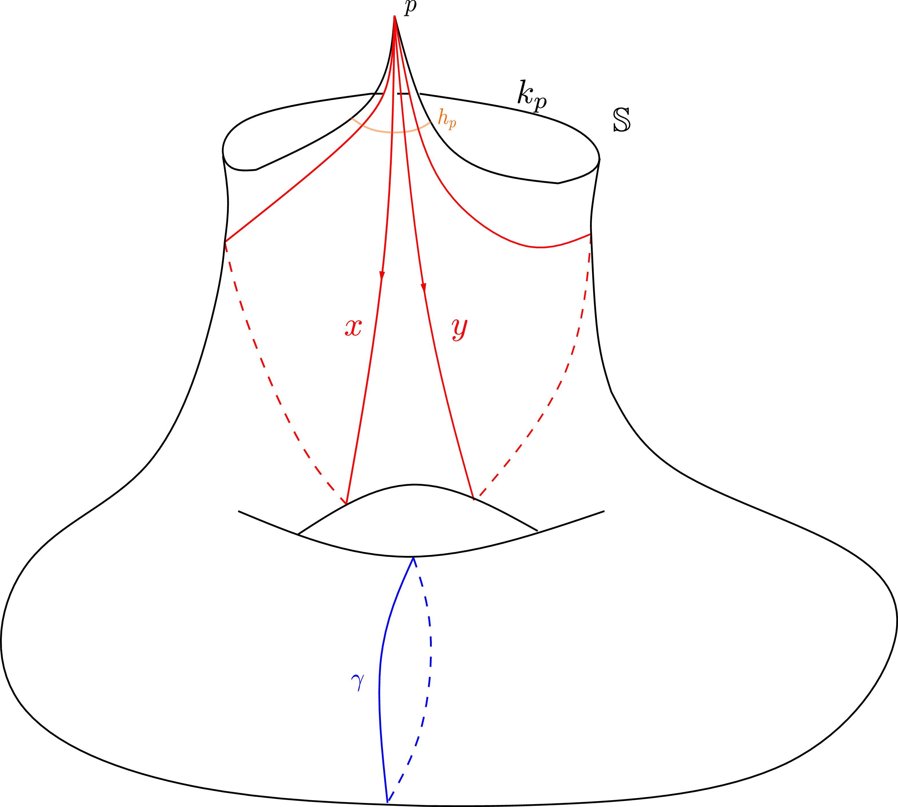
7.2 The once crowned torus with a single cusp↩︎
Let \({\Bbb S}\) be the once crowned torus with a cusp \(p\). Pick a non-peripheral simple geodesic \(\gamma\). The subgroup of the group \({\rm Mod}({\Bbb S})\) stabilizing the loop \(\gamma\) is isomorphic to \({\mathbb{Z}}\oplus {\mathbb{Z}}\). It is generated by the Dehn twists \({\rm D}_\gamma\) and \({\rm D}_{\rm C}\) along the loop \(\gamma\), and the neck loop for the crown \({\rm C}\). Denote by \(k_p\) the crown geodesic. Choose an embedded ideal triangle \(xyk_p\), see Figure 34. Figure 8 helps to visualize it. Any trouser leg contains the cusp \(p\). There are two trouser legs \({\rm T}({\gamma, x})\) and \({\rm T}({\gamma, y})\), see Figure 34. The Dehn twist \({\rm D}_\gamma\) preserves them. The subgroup \(\langle {\rm D}_{\rm C}\rangle\) generated by the Dehn twist \({\rm D}_{\rm C}\) acts freely on the set of trouser legs with two orbits \(\langle {\rm D}_{\rm C}\rangle \cdot {\rm T}({\gamma, x})\) and \(\langle {\rm D}_{\rm C}\rangle \cdot {\rm T}({\gamma, y})\). The moduli space \(\mathcal{M}_{{\Bbb S}}({\rm K}_p)\) with the fixed coordinate \({\rm K}_p\) at the geodesic \(k_p\) has dimension \(4\). It is parameterized by the \(\rm{K}\)-coordinates \({\rm K}_x\), \({\rm K}_y\), the length \(l_\gamma = \log{\rm L}_\gamma\) of the geodesic \(\gamma\), and the twist parameter \(\theta_\gamma\).
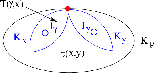
Applying Theorem 25 as illlustrated on Figure 35, we get \[\label{58} \begin{align} &\int_{{\cal M}_{\Bbb S}}W^\sharp_pe^{-W_{\Bbb S}}\Omega_{\Bbb S}=\\ &4\int_{\mathbb{R}^2_+} Q(\gamma,x) \cdot {\rm{Vol}}_{\mathcal{E}}{\cal M}_{{\rm T}(\gamma,x)}({\rm K}_x,l_\gamma) \cdot {\rm{Vol}}_{\mathcal{E}}{\cal M}_{{\Bbb S}- {\rm T}(\gamma,x)}({\rm K}_p, {\rm K}_x,l_\gamma)\cdot l_{\gamma} \cdot d l_{\gamma} \wedge d \log {\rm K}_x \\+& \int_{\mathbb{R}^2_+} S(x,y)\cdot {\rm{Vol}}_{\mathcal{E}}{\cal M}_{\tau(x,y)}({\rm K}_x, {\rm K}_y, {\rm K}_p) \cdot {\rm{Vol}}_{\mathcal{E}}{\cal M}_{{\Bbb S}-\tau(x,y)}({\rm K}_x, {\rm K}_y) \cdot d\log {\rm K}_x \wedge d\log {\rm K}_y. \end{align}\tag{111}\] The coefficient \(4\) reflects that the first integral in (111 ) is equal to the one obtained by changing \(x\to y\). According to (?? ) and (77 ) we have: \[Q(\gamma,x)={\rm K}_x^{\frac{1}{2}} {\rm L}_\gamma^{-\frac{1}{2}},\;\;\;\;\;\; S(x,y)= \left(\frac{{\rm K}_p}{{\rm K}_x {\rm K}_y}\right)^{-\frac{1}{2}}.\]
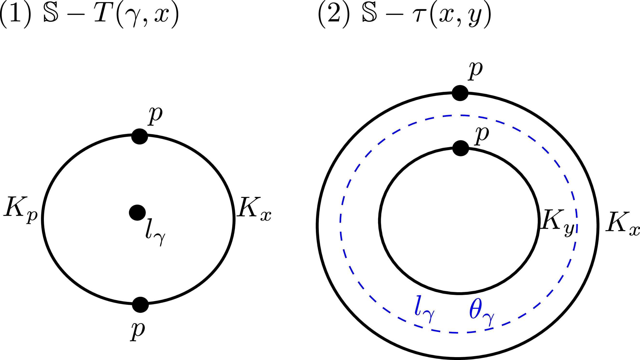
I) Let us elaborate the second line in (111 ). Recall that \[{\rm{Vol}}_{\mathcal{E}}{\cal M}_{ {\rm T}(\gamma,x)}({\rm K}_x,l_\gamma)\;\stackrel{(\ref{EXVT})}{=}\;{\rm exp}\left(-{\rm K}^{\frac{1}{2}}_x({\rm L}_\gamma^{\frac{1}{2}}+ {\rm L}_\gamma^{-\frac{1}{2}})\right).\] The surface \({\Bbb S}- {\rm T}(\gamma,x)\) is an annulus \({\rm A}_{0,2}\), see Figure 36 (1). We parameterize the space \({\cal M}_{{\Bbb S}- {\rm T}(\gamma,x)}\) as in Figure 36 (1). Using formula (101 ) for \({\rm{Vol}}_{\mathcal{E}}{\cal M}_{{\Bbb S}- {\rm T}(\gamma,x)}({\rm K}_p, {\rm K}_x,l_\gamma)\), we write the second line in (111 ) as
\[\label{58a} \begin{align} &4 \cdot \int_{\mathbb{R}^3_{>0}} {\rm K}_x^{\frac{1}{2}} {\rm L}_\gamma^{-\frac{1}{2}}\cdot {\rm exp}\Bigl( -({\rm K}^{\frac{1}{2}}_x +{\rm K}^{\frac{1}{2}}_y) ({\rm L}_\gamma^{\frac{1}{2}} + {\rm L}_\gamma^{-\frac{1}{2}} ) -W_\tau({\rm K}_p, {\rm K}_x, {\rm K}_y) \Bigr) \cdot l_{\gamma} d l_{\gamma} \wedge \frac{d{\rm K}_x}{{\rm K}_x}\wedge \frac{d{\rm K}_y}{{\rm K}_y}. \end{align}\tag{112}\]

II) Let us elaborate the last line in (111 ). The exponential volume of the moduli space for the triangle \(\tau(x,y)\): \[{\rm{Vol}}_{\mathcal{E}}{\cal M}_{\tau(x,y)}({\rm K}_x, {\rm K}_y, {\rm K}_p)\;\stackrel{(\ref{EXVt})}{=} \;\exp\left(-W_\tau({\rm K}_x, {\rm K}_y, {\rm K}_p)\right).\] The surface \({\Bbb S}- \tau(x,y)\) is an annulus \({\rm A}_{1,1}\), see Figure 36 (2). So using (107 ), the last line in (111 ) becomes an integral over \({\rm A},{\rm B}, {\rm K}_x, {\rm K}_y>0\): \[\label{101q} \begin{align} & \int \left(\frac{{\rm A}{\rm B}}{{\rm K}_p} \right)^{\frac{1}{2}} \;\frac{ {\rm exp}\Bigl(- W_\tau({\rm A},{\rm B},{\rm K}_x) - W_\tau({\rm A},{\rm B},{\rm K}_y)-W_\tau({\rm K}_x, {\rm K}_y, {\rm K}_p)\Bigr)}{ ({\rm L}_\gamma^{\frac{1}{2}} - {\rm L}_\gamma^{-{\frac{1}{2}} })} \frac{d {\rm A}}{{\rm A}} \wedge \frac{d {\rm B}}{{\rm B}} \wedge \frac{d {\rm K}_x}{{\rm K}_x}\wedge \frac{d {\rm K}_y}{{\rm K}_y}. \\ \end{align}\tag{113}\]
7.3 The McShane identity for a pair of pants with cusps↩︎
Let \({\Bbb S}\) be a pair of pants with one marked point on each boundary component as in Figure 38 (1). Let \(\gamma_p\), \(\gamma_q\), \(\gamma_r\) be the loops surrending the crown ends \(k_p\), \(k_q\), \(k_r\) respectively, whose Dehn twists generate the mapping class group \(\mathrm{Mod}({\Bbb S})\cong\mathbb{Z} \times \mathbb{Z} \times \mathbb{Z}\). Our goal is to describe all terms of the McShane identity for the cusp \(p\), and hence all terms of the unfolding formula. We consider all geodesics emitting from \(p\).
The bi-infinite geodesics \(k_q'\), \(k_r'\), \(k_p\) form a \(p\)-narrowest ideal triangle as in Figure 38 (2) with the potential \(\theta_b:=W_p(k_q', k_r')\) at the cusp \(p\). Any geodesic emitting from \(p\) within the arc between \(k_q'\) and \(k_r'\) hits the boundary \(k_p\). The annulus \({\rm A}^q_{1,1}\) is bounded by a bi-infinite geodesic \(k_q'\) and the crown end \(k_q\) with the potential \(W_{k_q'}\) at \(p\), while the annulus \({\rm A}^r_{1,1}\) is bounded by a bi-infinite geodesic \(k_r'\) and the crown end \(k_r\) with the potential \(W_{k_r'}\) at \(p\).

The Dehn twist of \(a\) by \(\gamma_p\) is denoted by \(\gamma_p a\). Then bi-infinite geodesics \(\gamma_p k_r'\), \(k_q'\), \(k_p\) form a \(p\)-narrowest ideal triangle as in Figure 39 (1) with the potential \(\theta_a:=W_p(\gamma_p k_r', k_q')\) at the cusp \(p\).

Any geodesic emitting from \(p\) within the arc between \(\gamma_p k_r'\) and \(k_q'\) hits the boundary \(k_p\). Similarly, the bi-infinite geodesics \(k_r'\), \(\gamma_p^{-1} k_q'\), \(k_p\) form a \(p\)-narrowest ideal triangle as in Figure 39 (2) with the potential \(\gamma_p^{-1} \theta_a:=W_p(k_r', \gamma_p^{-1} k_q')\) at the cusp \(p\). Any geodesic emitting from \(p\) within the arc between \(k_r'\) and \(\gamma_p^{-1} k_q'\) hits the boundary \(k_p\). Inductively, we have \[W_p=2 Q(\gamma_p, k_p)+ \sum_{i\in \mathbb{Z}} (\gamma_p^i\theta_a+W_{\gamma_p^i k_q'}+ \gamma_p^i\theta_b+W_{\gamma_p^i k_r'}).\]
Within \(\gamma_p^i {\rm A}_{1,1}^q\), let \(\{\ell_{i,q}^j\}_{j\in \mathbb{Z}}\) be a family of simple arcs connecting \(p\) and \(q\) where \(\ell_{i,q}^{j+1} = \gamma_q \ell_{i,q}^j\). Inside the ideal triangle \(\Delta_{i,q}^j\) formed by \(\ell_{i,q}^j\), \(\ell_{i,q}^{j+1}\) and \(k_q\), every geodesic emitting from \(p\) between \(\ell_{i,q}^j\) and \(\ell_{i,q}^{j+1}\) hits \(k_q\). Then \[W_{\gamma_p^i k_q'}\;=\;2 Q(\gamma_q, \gamma_p^i k_q') + \sum_{j\in \mathbb{Z}} W_p(\ell_{i,q}^j, \ell_{i,q}^{j+1} ).\] Similarly, we obtain \[W_{\gamma_p^i k_r'}\;=\;2 Q(\gamma_r, \gamma_p^i k_r') + \sum_{j\in \mathbb{Z}} W_p(\ell_{i,r}^j, \ell_{i,r}^{j+1} ).\] Combining the above three equations, we obtain the McShane identity \[\begin{align} \label{eqcpp1} W_p-2Q(\gamma_p, k_p)& \;= \;\sum_{i\in \mathbb{Z}} \gamma_p^i\theta_a+ \sum_{i\in \mathbb{Z}} \gamma_p^i\theta_b + 2 \sum_{i\in \mathbb{Z}} Q(\gamma_q, \gamma_p^i k_q')+ 2 \sum_{i\in \mathbb{Z}} Q(\gamma_r,\gamma_p^i k_r') \\& \;+ \;\sum_{i\in \mathbb{Z}} \sum_{j\in \mathbb{Z}} W_p(\ell_{i,q}^j, \ell_{i,q}^{j+1} )+ \sum_{i\in \mathbb{Z}} \sum_{j\in \mathbb{Z}} W_p(\ell_{i,r}^j, \ell_{i,r}^{j+1}). \end{align}\tag{114}\]
8 Exponential volumes and Whittaker–Hecke algebra for \({\rm SL}_2({\mathbb{R}})\)↩︎
Recall the three elementary decorated surfaces: the triangle \(\tau\), the trouser leg \({\rm T}\), and a pair of pants. The volume of the last is equal to \(1\). The exponential volumes of the first two are non-trivial functions \({\cal E}_\tau({\rm K}_1, {\rm K}_2, {\rm K}_3)\) and \({\cal E}_{\rm T}({\rm K}, {\rm L})\). The related \({\cal B}-\)function is the Bessel function: \[\label{BESS} {\cal B}_{\rm T}({\rm K}, s) = \int_{{\mathbb{R}}_{>0}} {\cal E}_{\rm T}({\rm K}, {\rm L}){\rm L}^{s/2}d\log {\rm L}\stackrel{\eqref{FBFa}}{=} 2J_s({\rm K}).\tag{115}\] We define an algebra \({\cal E}\), consisting of functions \(f\) on \({\mathbb{R}}_{>0}\) with exponential decay at infinity, with the product \(\ast\) given by \[\label{PFE9} (f\ast g)({\rm K}_3):= \int_{{\mathbb{R}}_{>0}\times {\mathbb{R}}_{>0}} {\cal E}_\tau({\rm K}_1, {\rm K}_2, {\rm K}_3)f({\rm K}_1)g({\rm K}_2) d\log{\rm K}_1 d\log {\rm K}_2.\tag{116}\]
Theorem 33. The product \(\ast\) is commutative and associative. Functions \({\cal B}_{\rm T}({\rm K}, s)\) satisfy the product formula \[\label{PF10} {\cal B}_{\rm T}({\rm K}_1, s)\cdot {\cal B}_{\rm T}({\rm K}_2, s) = \int_{{\mathbb{R}}_{>0}} {\cal E}_\tau({\rm K}_1, {\rm K}_2, {\rm K}_3){\cal B}_{\rm T}({\rm K}_3, s)d\log {\rm K}_3.\qquad{(36)}\] The function \({\cal B}_{\rm T}({\rm K}, s)\) provides a homomorphism \(\psi_s\) of the algebras \(({\cal E}, \ast)\) to \({\mathbb{C}}\): \[\label{PF13} \psi_{s}(f):= \int_{{\mathbb{R}}_{>0}} f({\rm K}){\cal B}_{\rm T}({\rm K}, s)d\log {\rm K}.\qquad{(37)}\]
Proof. The product \(\ast\) is commutative since the function \({\cal E}_\tau({\rm K}_1, {\rm K}_2, {\rm K}_3)\) is symmetric in \({\rm K}_1, {\rm K}_2, {\rm K}_3\).
The associativity. Recall the exponential volume form for the rectangle \(\square\): \[\label{EVFREC} e^{-W_\square}\Omega_\square({\rm K}_1, {\rm K}_2, {\rm K}_3, {\rm K}_4).\tag{117}\] There are two ways to cut the rectangle into two triangles, see Figure 40: \(\square = \tau_1 \cup \tau_2 = \tau_3\cup \tau_4\). So the cutting and gluing properties of exponential volume forms provide two presentations of the exponential volume form of the rectangle: \[\begin{align} (\ref{EVFREC}) = &{\cal E}_{\tau_1}({\rm K}_1, {\rm K}_2, {\rm K}) {\cal E}_{\tau_2}({\rm K}, {\rm K}_3, {\rm K}_4) d\log {\rm K}= {\cal E}_{\tau_3}({\rm K}_2, {\rm K}_3, {\rm K}) {\cal E}_{\tau_4}({\rm K}, {\rm K}_4, {\rm K}_1) d\log {\rm K}. \\ \end{align}\] Multiplying it by \(f_1({\rm K}_1)f_2({\rm K}_2) f_3({\rm K}_3)f_4({\rm K}_4)\) and integrating we get the associativity of the product \(\ast\).
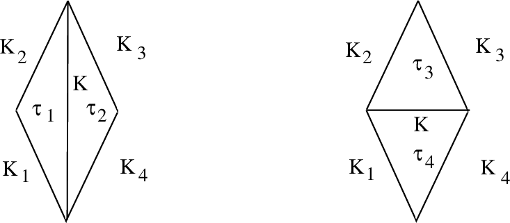
The product formula. Cut the disc \({\rm D}_1^*\) along the radius, getting a triangle \(\tau'\) with a vertex \(p\) corresponding to the puncture of \({\rm D}_1^*\). Let \({\cal T}_{\tau'}\) be the space parametrising ideal geodesic triangles \([a,b,p]\) with horocycles \(h_a, h_b\) at the vertices \(a,b\). The notation \(\tau'\) stresses that one of the cusps, the cusp \(p\), does not carry a horocycle. Pick any horocycle \(h_p\) at \(p\). Recall the signed geodesic length \(\kappa_{xy}\) between horocycles \(h_y\) and \(h_y\). The space \({\cal T}_{\tau'}\) carries a well defined function, independent of the choice of horocycle \(h_p\): \[\label{wdfT} \;{\rm L}_{\tau'}= e^{-(\kappa_{ap}-\kappa_{pb})}.\tag{118}\]
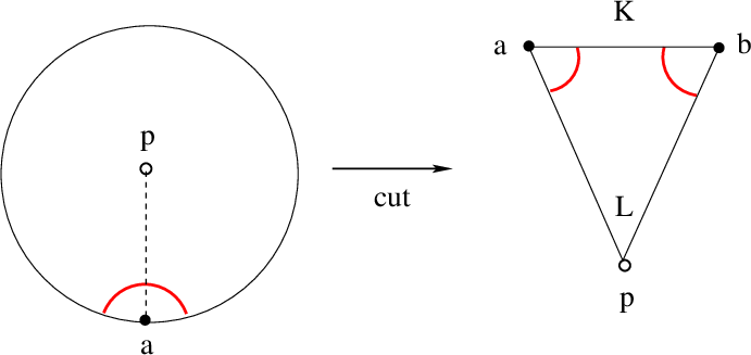
We fix the value of the coordinate \({\rm K}:= e^{-\kappa_{ab}}\). Then there is the exponential volume form \[\label{WWWa} e^{-W_{\tau'}}\Omega_{\tau'}({\rm K}) := e^{-W_{\tau'}}d\log {\rm L}_{\tau'}, \;\;\;\; W_{\tau'}= W_a+W_b.\tag{119}\]
Consider the space \({\cal T}_{\square'}\) parametrising ideal geodesic rectangles \((a,b,c,p)\) with horocycles \(h_a, h_b, h_c\) at the vertices \(a,b,c\). We fix the value of the coordinate \({\rm K}_1:= e^{-\kappa_{ab}}\) and \({\rm K}_2:= e^{-\kappa_{bc}}\). The space \({\cal T}_{\square'}\) carries a well defined function \({\rm L}_{\square'}\) similar to (118 ), and the volume form: \[{\rm L}_{\square'}:= e^{-(\kappa_{ap}-\kappa_{pc})}, \;\;\;\;\;\;\Omega_{\square'}(K_1, {\rm K}_2) := d\log {\rm K}\wedge d\log {\rm L}_{\square'}.\]
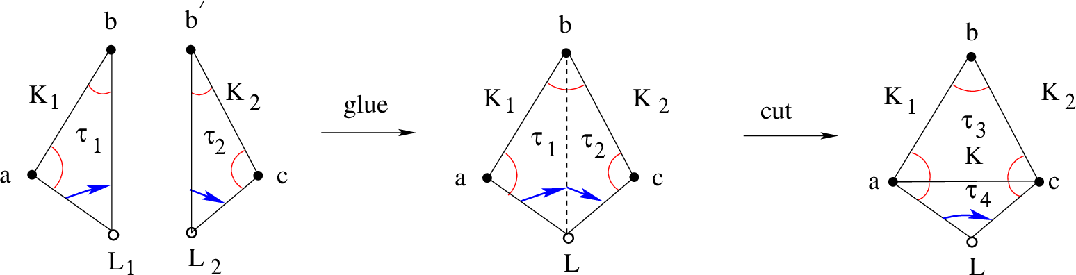
Take two triangles with horocyles \(\tau_1'=(a,b_1, p; h_a, h_{b_1})\) and \(\tau_2'= (b_2,c,p; h_{b_2}, h_c)\). Glue them along the sides \(b_1p\) and \(b_2p\) matching the horocyles \(h_{b_1}\) and \(h_{b_2}\), see Figure 42. We get a rectangle \(\square' = (a,b,c, p)\) with three horocycles \(h_a, h_b, h_c\). The gluing provides an isomorphism of spaces with volume forms: \[{\cal T}_{\square'} = {\cal T}_{\tau_1'}\times {\cal T}_{\tau_2'}; \;\;\;\Omega_{\square'}({\rm K}_1, {\rm K}_2) = \Omega_{\tau_1'}({\rm K}_1) \wedge \Omega_{\tau_2'}({\rm K}_2).\] Then we have the gluing conditions for the potentials and the functions \({\rm L}\):
\[W_{\square'} = W_{\tau_1} + W_{\tau_2} = W_{\tau_3} + W_{\tau_4},\;\;{\rm L}_{\square'} = {\rm L}_{\tau_1} {\rm L}_{\tau_2}.\] Therefore using (119 ) we have a factorization of the exponential volume form: \[\label{evfa} e^{-W_{\square'}}\Omega({\rm K}_1, {\rm K}_2) = e^{-W_{\tau_1}({\rm K}_1,{\rm L}_{\tau_1})} d\log({\rm L}_{\tau_1}) \wedge e^{-W_{\tau_2}({\rm K}_2, {\rm L}_{\tau_2})} d\log{\rm L}_{\tau_2}.\tag{120}\]
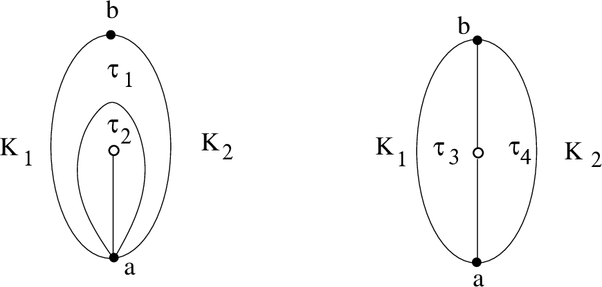
On the other hand, cutting the rectangle \(\square'\) by the diagonal \(ac\) into two triangles \(\tau_3\) and \(\tau_4\), see Figure 42, where \(\tau_3 = (a,b,c)\) with horocycles \(h'_a, h_b, h_c'\) and \(\tau'_4=(a,c, p)\) with horocycles \(h_a'', h_c''\), we get \[\label{evfb} e^{-W_{\square'} }\Omega({\rm K}_1, {\rm K}_2) = e^{-W_{\tau_3}({\rm K}_1, {\rm K}_2, {\rm K}) }\cdot e^{-W_{\tau_4}({\rm K}, {\rm L}_{\square'})} d\log {\rm L}_{\square'} \wedge d\log {\rm K}.\tag{121}\] Comparing (120 ) and (121 ) and multiplying by \({\rm L}_{\tau_1}^{s/2}{\rm L}_{\tau_2}^{s/2} = {\rm L}_{\square'}^{s/2}\) we get \[e^{-W({\rm K}_1; {\rm L}_{\tau_1})}{\rm L}_{{\tau_1}}^{s/2} d\log {\rm L}_{\tau_1} \wedge e^{-W_2({\rm K}_2; {\rm L}_{\tau_2} )}{\rm L}^{s/2}_{\tau_2} d\log {\rm L}_{\tau_2} = {\cal E}_{\tau_3}({\rm K}_1, {\rm K}_2, {\rm K}) \cdot e^{-W_{\tau_4}({\rm K},{\rm L}_{\square'})} {\rm L}_{\square'}^{s/2}d\log ({\rm L}_{\square'}) \wedge d\log {\rm K}.\] Integrating these exponential volume forms we get the product formula, see Figure 43.
The multiplicativity of the map \(\psi_s\). Equality (?? ) follows from (116 ) and (?? ): \[\label{PF3} \begin{align} \kappa_{s}(f\ast g) = &\int_{{\mathbb{R}}_{>0}} (f\ast g)({\rm K}_3) {\cal B}_{\rm T}({\rm K}_3, s) d\log {\rm K}_3 \\ =&\int_{{\mathbb{R}}_{>0}} {\cal E}_\tau({\rm K}_1, {\rm K}_2, {\rm K}_3) f({\rm K}_1)g({\rm K}_2) {\cal B}_{\rm T}({\rm K}_3, s) d\log {\rm K}_1 d\log {\rm K}_2 d\log {\rm K}_3 \\ =&\int_{{\mathbb{R}}_{>0}} {\cal B}_{\rm T}({\rm K}_1, s){\cal B}_{\rm T}({\rm K}_2, s) f({\rm K}_1)g({\rm K}_2) d\log {\rm K}_1 d\log {\rm K}_2 \\ =&\kappa_{s}(f) \cdot \kappa_s(g). \; \\ \end{align}\tag{122}\] ◻
Few comments are in order.
Cutting the decorated surface \({\rm D}_2^*\) along the radius connecting the special point and the puncture we get the rectangle \(\square'\). The product formula just means that calculating the exponential volume of the moduli space for \({\rm D}_2^*\) using the two triangulations of \({\rm D}_2^*\) on Figure 43 leads to the same result.
The Cartan group \({\rm H}({\mathbb{R}})\) of \({\rm PGL}_2({\mathbb{R}})\) has two components. One of them is the positive part of the Cartan group \({\rm H}({\mathbb{R}}_{>0}) = {\mathbb{R}}^\times_{>0}\). Let \({\rm N}\subset {\rm PGL}_2\) be the upper triangular unipotent subgroup, so \({\rm N}({\mathbb{R}}) = {\mathbb{R}}\). Let \(\psi(a) = e^{2\pi i a}\) be an additive character of \({\rm N}({\mathbb{R}})\). The Laplace operator \(\Delta_{{\rm sl}_2}\) is the generator of the center of the universal enveloping algebra \({\cal U}({\rm sl}_2({\mathbb{R}}))\).
Recall the Whittaker function \({\cal S}(g, s)\), where \(g \in {\rm PGL}_2({\mathbb{R}})\), of the principal series representation \(V_s\) of \({\rm PGL}_2({\mathbb{R}})\). It has the following properties:
The function \({\cal S}(g, s)\) is \(({\rm N}({\mathbb{R}}), \psi)\) bi-invariant: \[{\cal S}(n_1gn_2, s) = \psi(n_1)\psi(n_2){\cal S}(g, s)\;\;\;\;\;\;\forall n_{1}, n_2 \in {\rm N}({\mathbb{R}}).\]
Its restriction to the coset \(w_0{\rm H}({\mathbb{R}}_{>0})\) of the positive Cartan subgroup is the Bessel function: \[{\cal S}(w_0h({\rm K}), s) = {\cal B}_{\rm T}({\rm K}, s), \;\;\;{\rm K}\in {\mathbb{R}}^\times_{>0}, \;\;\;\;\;\;\;h({\rm K}):= \begin{pmatrix} {\rm K}& 0 \\ 0 & {\rm K}^{-1}\\ \end{pmatrix}, \;\;w_0= \begin{pmatrix} 0 & 1 \\ -1 & 0\\ \end{pmatrix}.\]
The function \({\cal S}(g, s)\) is an eigenfunction of the Laplace operator \(\Delta_{{\rm sl}_2}\).
Let us elaborate the analogy with the classical zonal spherical functions [16].
The classical Hecke algebra \({\cal H}_{\rm SO(2)}\). It is given by compactly supported functions on \({\rm SL}_2({\mathbb{R}})\) which are left and right invariant under the action of the maximal compact subgroup \({\rm SO}(2)\subset {\rm SL}_2({\mathbb{R}})\). The product is given by the convolution. It is associative and commutative. Any irreducible unitary spherical principal series representation \(V_s\) of the group \({\rm SL}_2({\mathbb{R}})\) contains a unique normalised spherical vector \(v_s\). The corresponding matrix element is called the zonal spherical function: \[{\cal S}_{\rm SO(2)}(g, s):= \langle v_s, gv_s\rangle.\] It is an eigenfunction of the Laplace operator, bi-invariant under the action of the group \({\rm SO}(2)\). So it is determined by its restriction to the subgroup \({\rm H}({\mathbb{R}})\). Therefore the product in the algebra \({\cal H}_{\rm SO(2)}\) can be written in terms of the functions on \({\rm H}({\mathbb{R}})\) using a certain kernel \(a({\rm K}_1, {\rm K}_2, {\rm K}_3)\): \[\label{SU2aa} (f\ast g)({\rm K}_3):= \int_{{\mathbb{R}}^\times\times {\mathbb{R}}^\times} {a}({\rm K}_1, {\rm K}_2, {\rm K}_3)f({\rm K}_1)g({\rm K}_2) d\log{\rm K}_1 d\log {\rm K}_2.\tag{123}\]
The zonal function \({\cal S}_{\rm SO(2)}({\rm K}, s)\) satisfies the product formula \[\label{PF10a} {\cal S}_{\rm SO(2)}({\rm K}_1, s)\cdot {\cal S}_{\rm SO(2)}({\rm K}_2, s)= \int_{{\mathbb{R}}^\times} {a}({\rm K}_1, {\rm K}_2, {\rm K}_3) {\cal S}_{\rm SO(2)}(g, s)d\log {\rm K}_3.\tag{124}\] It provides a homomorphism of the algebras \(({\cal H}_{\rm SO(2)}, \ast)\) to \({\mathbb{C}}\): \[\label{PF13a} \varphi_{s}(f):= \int_{{\mathbb{R}}^\times} f({\rm K}){\cal S}_{\rm SO(2)}({\rm K}, s)d\log {\rm K}, \;\;\;\;\varphi_{s}(f\ast g) = \varphi_{s}(f)\varphi_{s}(g).\tag{125}\]
Conclusion. The algebra \({\cal E}\) is the analog of the Hecke algebra \({\cal H}_{\rm SO(2)}\) where the \({\rm SO}_2\) bi-invariance is replaced by the \(({\rm N}({\mathbb{R}}), \psi)\) bi-invariance. However the subgroup \({\rm N}({\mathbb{R}})\) is not compact, and so the convolution of \(({\rm N}({\mathbb{R}}), \psi)\) bi-invariant functions is divergent. Nevertheless the restriction to the \(w_0-\)coset of the positive part of the Cartan torus is well defined, and there is a commutative algebra with exactly the same properties, which we call the positive Hecke-Whittaker algebra.
The positive Hecke-Whittaker algebra \({\cal E}\) for \({\rm PGL}_2({\mathbb{R}})\) is given by the exponential volumes of elementary decorated surfaces. The exponential volumes of moduli spaces for all decorated surfaces, together with the unfolding formula, provide an extension of the algebra \({\cal E}\) to all decorated surfaces.
9 Birman–Series theorem for ideal hyperbolic surfaces↩︎
The main result of the Appendix is the following theorem, generalising the Birman–Series theorem [22] to ideal hyperbolic surfaces.
Theorem 34. Given an ideal hyperbolic structure on the decorated surface \({\Bbb S}\), let \(\mathcal{G}\) be the union of all bi-infinite geodesics without self-intersection. Then the area of \(\mathcal{G}\) with respect to the measure on the surface induced by the hyperbolic structure is equal to zero.
Let us start with the collar lemma. Given \(R>0\) and a cusp/puncture \(p\), there is a unique horoarc/horocycle \(h_R\) with the length \(R\). Let us define the collar neighbourhood \(C_R\) be the annular neighbourhood region bounded by \(h_R\).
Lemma 17. Given an ideal hyperbolic surface, for any cusp/puncture \(p\), there exists a collar neighborhood \(C_r\) of a cusp/puncture \(p\) such that for any bi-infinite geodesic \(\ell\) entering and exiting \(C_r\), the geodesic \(\ell\) has self-intersection.

Proof. Let us choose some horoarc/horocycle \(h_R\) for \(R>0\). Since the collar neighbourhood \(C_R\) is infinitely long, we can choose a smaller collar neighbourhood \(C_r\subset C_R\) such that the distance between \(h_r\) and \(h_R\) is at least \(R/2\). If a geodesic \(\ell\) enters and exits \(C_r\) and does not have self-intersection, then \(C_r\cap \ell\) contains at least two different points as in Figure 44 (1)(2). We define \(\ell^+\) (\(\ell^-\) resp.) to be the geodesic ray starting from the first (last resp.) intersection point of \(\ell \cap C_r\) towards the (opposite resp.) direction of \(\ell\). We claim that both \(\ell^+\) and \(\ell^-\) must leave \(C_R\) for any of the two directions. If \(\ell^{\pm}\) does not leave \(C_R\), the ideal end point of any lift of \(\ell^{\pm}\) is the unique ideal boundary point of the horodisk in the universal cover as in Figure 44 (3). This characterizes \(\ell^{\pm}\) as a geodesic going straight up to the cusp, and thus hitting every horocycle at most once. This is a contradiction as \(\ell^{\pm}\) meets \(C_r\) in two places. Hence both \(\ell^+\) and \(\ell^-\) must leave \(C_R\). Let \(\bar{\ell}\) be the subarc of \(\ell\) which lies completely within \(C_R\), has both its endpoints on \(h_R\), and enters and exits \(C_r\). Since \(\bar{\ell}\) has two subarcs between \(h_r\) and \(h_R\), it has length at least \(R\). On the other hand, the geodesic arc \(\bar{\ell}\) is endpoint-fixing homotopic to a horocyclic path along \(h_R\) without wrapping around \(h_R\). This implies the length of \(\bar{\ell}\) is strictly less than \(R\), leading to a contradiction. We conclude that any geodesic \(\ell\) entering and exiting \(C_r\) has self-intersection. ◻
As a consequence, any geodesic in \(\mathcal{G}\) lies in a compact set \(Q={\Bbb S}-\cup_p C_r\). Now, we fix an ideal triangulation \(\mathcal{T}\) of the ideal hyperbolic surface. The ideal triangulation \(\mathcal{T}\) cuts any geodesic in \(\mathcal{G}\) into segments. Then we define \(\mathcal{G}(N)\) to be the set of geodesic arcs in \(\mathcal{G}\) that are cut up into \(N\) geodesic segments by \(\mathcal{T}\).
Corollary 3. There exists a constant \(C>0\), such that for any \(\gamma \in \mathcal{G}(N)\), we have the length \(l_\gamma\geq C \cdot N\) for any \(N\geq 1\).
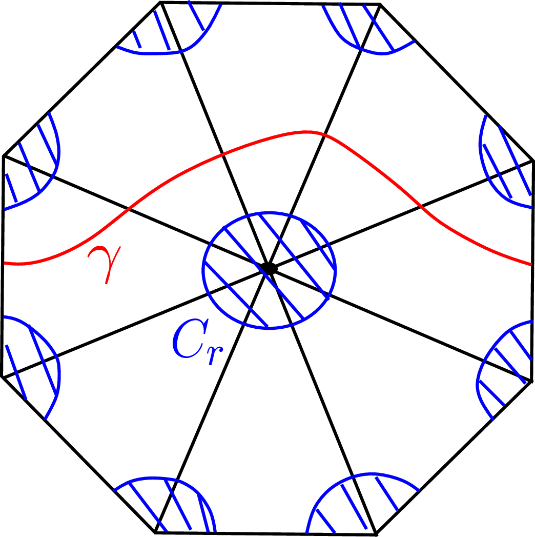
Proof. Any ideal triangle of the ideal triangulation \(\mathcal{T}\) is cut into three compact intervals by \(\cup_p C_r\). By Lemma 17, the length of a segment of \(\gamma \in \mathcal{G}(N)\) is determined by the pair of points on two of these three compact intervals. Since there are only finitely many ideal triangles, the length of a segment of \(\gamma \in \mathcal{G}(N)\) is a function on a compact set. Thus the length of a segment is bounded below by a constant \(C>0\). Hence \(l_\gamma\geq C \cdot N\). ◻
Proof of Theorem 34. Given an ideal triangulation \(\mathcal{T}\) of the ideal hyperbolic surface, any homotopy class \([\gamma]\in [\mathcal{G}(N)]\) is determined by
the multiset of \(N\) segments in \([\mathcal{G}(1)]\), thus \(x_1+\ldots+ x_{\#[\mathcal{G}(1)]}=N\) for \(x_i\) being the number of segments in these \(N\) segments of the given type;
the starting and ending segments of \([\gamma]\). We have
\[\#[\mathcal{G}(N)]\leq N^2 \cdot \tbinom{\#[\mathcal{G}(1)]+N-1}{N-1} =p_0(N),\] where \(p_0\) is a polynomial in \(N\).
Consider one fundamental domain \(F\) of the universal cover of the ideal hyperbolic surface in the Poincaré disk model. Let \(\tilde{\mathcal{T}}\) be the universal cover of the ideal triangulation \(\mathcal{T}\). Then \(\tilde{\mathcal{T}}\) cuts \(F\) into finitely many ideal triangles \(F\backslash \tilde{\mathcal{T}}=\cup_{i=1}^l \Delta_i\). \[I=\{\sigma=\tilde{\gamma}\cap \Delta_i \;|\; \text{ for some } i=1,...,l, \;\;\tilde{\gamma} \text{ lift of } \gamma \in \mathcal{G}\}.\] To prove the theorem is equivalent to prove the Euclidean area of \(I\) is zero. For any integer \(N>0\), any \(\sigma \in I\) is
uniquely expressed as the \((N+1)\)-th segment of \(\gamma \in \mathcal{G}(2N+1)\);
only one side of \(\sigma\) could extend to \(N\) segments, while the other side ends at some cusp/puncture;
both sides end at some cusp/puncture before \(N\) segments.
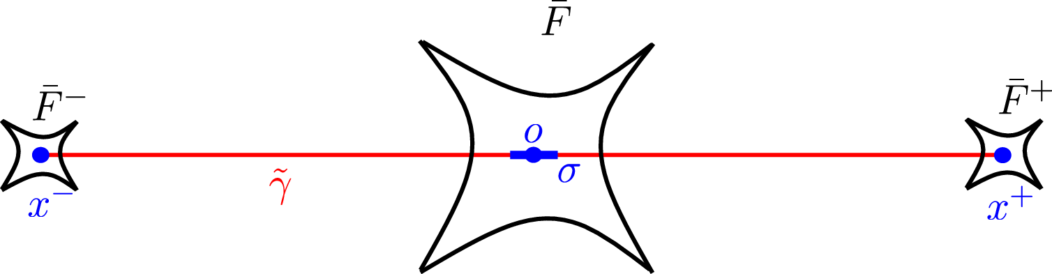
For Case (1), consider the lift \(\tilde{\gamma}\) of \(\gamma\) where \(\sigma \subset \tilde{\gamma}\) as in Figure 46. The segment \(\sigma\) is contained in the closure \(\bar{F}\) of the fundamental domain \(F\). Let \(x^-\) and \(x^+\) be two end points of \(\gamma\) which are contained in two fundamental domains \(\bar{F}^-\) and \(\bar{F}^+\) respectively. Choose any point \(o\in \sigma\), by Corollary 3, we have \(d(x^-,o)\geq C\cdot N\) and \(d(x^+,o)\geq C\cdot N\). The Euclidean diameter \(\rm{diam}_E{\bar{F}}\) of \(\bar{F}\) is finite in the Poincaré disk model. Since the ideal hyperbolic surface has negative constant curvature \(-1\), we get the Euclidean diameters \(\rm{diam}_E{\bar{F}^-}\leq C_0 e^{-C_1 N}\) and \(\rm{diam}_E{\bar{F}^+}\leq C_0 e^{-C_1 N}\) for some constant \(C_0, C_1>0\). Then for any representive \(\gamma\) of \([\gamma]\), we cover any \(\sigma(\subset\gamma)\) by the convex hull \(\square_{[\gamma]}\) of \(\bar{F}^-\) and \(\bar{F}^+\). The Euclidean area of \(\square_{[\gamma]}\) is less than \(C_2 e^{-C_1 N}\) for some constant \(C_2>0\). Since \[\lim_{N\rightarrow +\infty} \# [\mathcal{G}(2N+1)] \cdot C_2 e^{-C_1 N}=0,\] for any integer \(N>0\), we could cover all these kinds of \(\sigma\) by all these convex hulls.
For Case (2), let \(\sigma\subset \gamma\) and \(\gamma\in \mathcal{G}(M)\) for \(M\leq 2N\), where \(\gamma\) is a geodesic ray ending at the cusp/puncture \(p\) and \(\sigma\) is the \((N+1)\)-th segment of \(\gamma\). We cover \(\gamma\) by the convex hull of \(\bar{F}^-\) and \(p\) which has the Euclidean area less than \(C_2 e^{-C_1 N}\). Then we have \[\lim_{N\rightarrow +\infty} \sum_{M=N+1}^{2N} \# [\mathcal{G}(M)] \cdot C_2 e^{-C_1 N}=0,\]
For Case (3), we cover these finitely many bi-infinite geodesics by themselves.
Combining all these cases, we cover \(I\) by a sequence of measuable sets \(U_N\) such that the Euclidean area of \(U_N\) converges to zero. ◻
10 Relative volume forms↩︎
Recall the relative volume form in 48 . Let \(S\) be a sphere with \(n\) punctures, \(\ell\) a simple loop on \(S\), and \(S':=S-\ell\). The monodromy map \({\cal X}_S\longrightarrow({\mathbb{C}}^\times)^n\) maps an element in \({\cal X}_S\) into \(({\rm L}_1,..., {\rm L}_n)\) where, given any ideal triangulation, the \({\rm L}_i\) is the product of the cluster \(\mathcal{X}\)-coordinates at the edges sharing the \(i-\)th puncture. The \({\rm L}_i\) does not depend on the triangulation. The fibers of the monodromy map \({\cal X}_S\longrightarrow({\mathbb{C}}^\times)^n\) are the generic symplectic fibers on the cluster Poisson space \({\cal X}_S\). Given a point of \({\cal X}_S(\mathbb{R}_{>0})\), we have \({\rm L}_i=e^{l_i}\) where \(l_i\in \mathbb{R}\) is the signed boundary geodesic length. Let \(l\) be the length of \(\ell\) and \(\theta\) the twist parameter of \(\ell\). Let \({\rm L}=(l_1,...,l_n)\) and \({\rm L}'=(l_1,...,l_n, l,l)\).
::: {#WP=cl .lemma} Lemma 18. The cluster volume forms \(\Omega_S({\rm L})\) on \({\cal X}_S(\mathbb{R}_{>0})({\rm L})\) and \(\Omega_{S'}({\rm L}')\) on \({\cal X}_{S'}(\mathbb{R}_{>0})({\rm L}')\) are related by \[\Omega_S({\rm L}) = \frac{1}{2} \cdot \Omega_{S'}({\rm L}') \wedge dl \wedge d\theta.\]
Proof. By Wolpert’s formula [28], we have the Weil–Petersson form and the corresponding volume form: \[\begin{align} &\omega_{\rm WP} = \sum_{i=1}^{n-3} d l_i\wedge d\theta_i,\;\;\; \Omega^{\rm WP}_S({\rm L}) := \omega_{\rm WP}^{n-3}/(n-3)!.\\ &\Omega^{\rm WP}_S({\rm L}) = \Omega^{\rm WP}_{S'}({\rm L}') \wedge dl \wedge d\theta.\\ \end{align}\]

Let us relate the cluster volume form \(\Omega_S({\rm L})\) to \(\Omega^{\rm WP}_S({\rm L})\). Given any ideal triangulation as in Figure 47, we have \[l_1=x_1, l_n=x_{n-1},\] \[l_i=2 z_{i-1}+x_{i-1}+x_{i}+y_{i-1}+y_{i}\] for \(i=2,..., n-1\) with \(y_1=y_{n-1}:=0\). By definition \[\Omega_S({\rm L})\wedge \bigwedge_{i=1}^{n} d l_i=2\bigwedge_{i=2}^{n-2} \left(d x_i \wedge d y_i \right) \bigwedge_{i=1}^{n-2}d z_i \wedge d x_1 \wedge d x_{n-1}.\] Thus \[\Omega_S({\rm L})= \frac{1}{2^{n-3}}\bigwedge_{i=2}^{n-2} \left(d x_i \wedge d y_i \right).\] So we get \[\omega_{\rm cl}= \frac{1}{2} \sum_{i=2}^{n-2} d x_i \wedge d y_i.\] By [2], \(2\omega_{\rm cl} = \omega_{\rm WP}\). So we obtain \[\label{WPCLn} \Omega^{\rm WP}_S({\rm L}) = \omega_{\rm WP}^{n-3}/(n-3)!=(2\omega_{\rm cl})^{n-3}/(n-3)!=\bigwedge_{i=2}^{n-2} \left(d x_i \wedge d y_i \right)=2^{n-3}\Omega_S({\rm L}) .\tag{126}\] Since \(\alpha\) cuts \(S\) into \(S'=S_{0,n_1}\cup S_{0,n_2}\) where \(n=n_1+n_2-2\), we obtain \[\Omega_S^{\rm WP}({\rm L})=\Omega_{S_{0,n_1}}^{\rm WP}({\rm L}'') \wedge \Omega_{S_{0,n_2}}^{\rm WP}({\rm L}''') \wedge d l_\alpha \wedge d \theta_\alpha.\] Thus \[2^{n-3}\Omega_S({\rm L})= 2^{n_1-3}\Omega_{S_{0,n_1}}({\rm L}'') \wedge 2^{n_2-3}\Omega_{S_{0,n_2}}({\rm L}''') \wedge d l_\alpha \wedge d \theta_\alpha,\] which implies \[\Omega_S({\rm L}) = \frac{1}{2}\cdot \Omega_{S'}({\rm L}') \wedge dl \wedge d\theta.\] ◻
:::::::::::
References↩︎
The reason for the factor \(-1\) will be clarified later, see Definition 8.↩︎
Using [4], we have \(d_S=2^{-2g+3-n}= 2^{\chi_S+1}\). If \(g=0\), see also formula (126 ) in Appendix 10.↩︎
The modified Bessel function of the second kind is often denoted by \(K_s(z)\). We have \(J_s(z) = 2 K_{-s}(2\sqrt{z})\).↩︎
Givental [9] addressed the case of the flag variety for \({\rm GL}_k\), rather than just \({\rm P}^1\).↩︎
The extra factor \(2^{\pi_0({\Bbb S})}\) spares us from extra factor \(2\) in Lemma 6 appearing when the edge \({\rm E}\) there is separating. However it results in the extra factor \(2\) in front of the Bessel function in (65 ). Note that the volume form with/without the extra factor is multiplicative: \(\Omega_{{\Bbb S}_1\cup {\Bbb S}_2} = \Omega_{{\Bbb S}_1}\wedge \Omega_{{\Bbb S}_2}\).↩︎
The \({\rm K}\) in \(\Omega_{\Bbb S}({\rm K})\) indicates that the \({\rm K}-\)coordinates on the decorated surface \({\Bbb S}\) are frozen.↩︎
Here \(\delta(f) \Omega\), where \(\Omega\) is a volume form on an \(n-\)dimensional manifold, is the volume form on the hypersurface \(f=0\) obtained as follows: we find an \((n-1)-\)form \(\omega\) such that \(df \wedge \omega = \Omega\), and restrict \(\omega\) to the hypersurface \(f=0\). The result is independent on the choice of \(\omega\), see [7].↩︎
Strictly speaking, the relative form is the form \(\Omega^\delta_{{\Bbb S}'}({\rm K}_{\rm E})\), restricted to the fiber \({\rm K}_{\rm E}=C\).↩︎
The factor \(2\) comes from the comparision between the Weil–Petersson form [2] and the cluster Poisson structure.↩︎
The volume form is obtained by dividing \(d\log {\rm B}\wedge d\log {\rm X}\) by \(d\log {\rm K}= d\log ({\rm X}/{\rm B}^2)\). So it is \(d\log {\rm B}\).↩︎
We change the terminology pair of half-pants in [23] to trouser leg.↩︎
Here we abuse the notation by denoting by \({\cal M}_S\) the space \({\cal M}_S({\mathbb{R}}_{>0})\), and by \({\cal M}^{\rm en}_S\) the space \({\cal M}^{\rm en}_S({\mathbb{R}}_{>0})\).↩︎
Note that \(\sigma_S = \frac{1}{2}\rho_S\) where \(\rho_S\) is the constant used by Kontsevich. The factor \(\frac{1}{2}\) is forced by the factor \(2= 2^{\pi_0(S)}\) in the definition (?? ) of the volume form \(\Omega_S\), and hence of \(\Omega^t_S\). Note that since \(S\) is connected, \(\pi_0(S) =1\).↩︎
See (98 ) for the modified coefficients \({\cal V}^*_{g, d_1, ..., d_m}\) for the tropical volume polynomial.↩︎