1 Introduction↩︎

Adversarial training [1], which uses projected gradient descent (PGD) to solve a minimax optimization objective, remains the most widely adopted algorithmic framework for training neural networks to be resilient to inputs crafted with small perturbations intended to fool the model [2]. Despite its prevalence, adversarial training exhibits a striking failure mode: robust test accuracy can deteriorate late in training—often immediately after a learning rate decay—even as the robust training loss continues to decrease. This phenomenon, known as robust overfitting [3], suggests that fitting the training objective does not necessarily translate into improved robust generalization on unseen data. To address the issue, various techniques have been proposed [4]–[6], yet a satisfying mechanistic interpretation of the phenomenon is lacking. While many heuristic robustness measures have been proposed, no single one can serve as a universal, reliable indicator of the model’s robust generalization capability [7].

The surprising robust overfitting phenomenon and its complexity have motivated theoretical studies [8]–[14] to analyze the factors that influence adversarially robust generalization by adapting classical frameworks such as PAC-Bayes and algorithmic stability. Nevertheless, the worst-case robustness guarantees derived from these studies are often loose and rely on strong assumptions that may not reflect the actual behavior of algorithms used in practice. Moreover, these bounds are usually static, designed to certify a predictor at a fixed model checkpoint, but are insufficient to characterize the time-varying dynamics of adversarial training, which is essential to fully understand robust overfitting.

In this work, we argue that robust overfitting is driven by a transient imbalance between loss curvature and stochastic noise as the model navigates the adversarial loss landscape through stochastic gradient descent (SGD). To uncover the underlying mechanism, we adopt the PAC-Bayesian framework and model the SGD dynamics of adversarial training algorithms as a discrete-time dynamical system (Section 4.1). By treating the iterative parameter distribution as an implicit posterior, we derive closed-form solutions that characterize how its mean and covariance evolve with learning rate, local curvature, and gradient-noise dynamics, which yield schedule-aware, time-varying robust generalization bounds tailored for different training stages of interest (Section 4.2). Based on an efficient spectral estimation protocol, we empirically estimate the quantities identified by the theory by tracking the per-epoch Hessian and gradient-noise dynamics across different learning algorithms, thereby characterizing the driving factors associated with adversarially robust generalization (Section 5). Together, our analyses support a time-varying mechanistic interpretation of robust overfitting: a sharp learning-rate decay leads to posterior contraction along sharp directions, benefiting robust optimization while lowering the curvature-weighted variance during the initial transient phase (corresponding to the early jump of training and testing robust accuracy); however, the Hessian eigenvalues keep increasing as adversarial training prolongs, which eventually boosts the curvature-weighted variance despite the contracted posterior and adversely affects the model’s robust generalization (corresponding to the gradual degradation of robust test accuracy in later epochs).

Our main contributions are summarized as follows:

1. By modeling momentum SGD as a dynamical system, we prove PAC-Bayesian robust generalization bounds for different learning stages of adversarial training. As a byproduct, our method can explicitly track the time-varying evolution of the posterior mean and covariance.

2. Through empirical estimation of the spectral quantities reflected in the bound, we provide a time-resolved diagnostic account of robust overfitting, illustrating how learning-rate decay, progressive sharpening, and posterior contraction jointly shape robust generalization.

3. We conduct controlled experiments to analyze the diagnostic patterns across various learning algorithms, suggesting that adversarial weight perturbation [5] may overly penalize Hessian eigenvalues.

2 Related Work↩︎

Robust Overfitting. Since the initial discovery of adversarial examples [2], numerous methods have been proposed to improve model robustness [15]–[18]. Among them, adversarial training (AT), a minimax optimization framework that employs projected gradient descent (PGD), is most popular [1]. However, AT exhibits a recurring failure mode: robust test accuracy can drop late in training—often right after learning rate decay—even as the robust training loss continues to decrease, a phenomenon termed robust overfitting [3]. Empirical remedies span three main categories: objective-based methods like TRADES [4], [19] redesign the training optimization objective, geometry-aware approaches like adversarial weight perturbation (AWP) [5], [20], [21] penalize the model’s sharpness for finding flatter solutions, and augmentation-based schemes [6], [22] incorporate extra data in adversarial training. Despite improvements, the above techniques are all empirical, which lacks a unified, mechanistic interpretation of the robust overfitting phenomenon.

Adversarially Robust Generalization. Existing literature has analyzed robust generalization using various theoretical tools. A line of work adapted the classical PAC-Bayes framework [23]–[25] to derive posterior-based robust generalization bounds [9], [10], [26], [27], often relating the KL-divergence complexity term to flatness-based measures. Another line of research studied adversarially robust generalization from the perspective of algorithmic stability [8], [14], [28], which captures a learning algorithm’s insensitivity to small perturbations in the training dataset. Additionally, [11] extended neural tangent kernel (NTK) analysis to AT, deriving closed-form dynamics under squared loss for neural networks with infinite width, while [12] focused on characterizing the impact of individual training instances on robust overfitting. Despite rigorous proofs, most theories rely on assumptions that deviate from practice. Even when assumptions are acceptable, the resulting bounds are often loose and cannot tightly explain the empirical robust overfitting curves. These observations highlight a critical limitation: existing studies focus on static worst-case guarantees; however, robust generalization requires understanding the model’s internal dynamics, suggesting the need for better analytical tools to characterize the actual adversarial training dynamics.

SGD Dynamics. Recently, a line of literature has proposed studying standard deep learning generalization by modeling SGD as a discrete-time stochastic dynamical system [29]–[31]. In particular, they showed how the learning rate, loss curvature, and gradient noise structure jointly shape parameter fluctuations, which can be used to derive an exact analytical form of the stationary distribution and explain how SGD escapes from sharp minima. Compared with prior literature that uses continuous-time SDEs or Langevin approximations [32], [33], this line of work accounts for the learning step size and minibatch stochastic noise, providing more realistic predictions for SGD dynamics and implicit regularization. We leverage recent advances in modeling SGD dynamics to characterize time-resolved PAC-Bayesian robust generalization bounds for adversarial training, offering a principled framework for understanding robust overfitting.

3 Preliminaries↩︎

Adversarial Risk. We work with the following theoretical definition of adversarial risk, which often serves as the basis for evaluating an ML model’s robustness against worst-case input perturbations [1], [3].

Note that when \(\epsilon = 0\), adversarial risk reduces to the standard notion of risk. In line with the existing literature, we focus on the most widely considered \(L_p\) perturbations. Correspondingly, the adversarial robustness of an ML model \(f_{\boldsymbol{w}}\) can be understood as \(1-\mathcal{R}_{\epsilon}(\boldsymbol{w})\). According to Equation 1 , one can show that adversarial risk is mathematically equivalent to \(\mathbb{E}_{(\boldsymbol{x},y)\sim\mathcal{D}} [\max_{\|\boldsymbol{\delta}\|_p\le \epsilon} \mathbb{1}\{f_{\boldsymbol{w}}(\boldsymbol{x}+\boldsymbol{\delta})\ne y\}]\).

Adversarial Training. To effectively train robust models with low adversarial risk, adversarial training is the most popular framework [1], [15]. Given a set of examples \(\mathcal{S}\) i.i.d. sampled from the underlying distribution \(\mathcal{D}\), adversarial training is designed to minimize the following empirical adversarial loss: \[\begin{align} \label{eq:def32empirical32adv32loss} \hat{\mathcal{L}}_{\epsilon}(\boldsymbol{w}) = \frac{1}{|\mathcal{S}|} \sum_{(\boldsymbol{x},y)\in\mathcal{S}} \bigg[ \max_{\|\boldsymbol{\delta}\|_p \leq \epsilon} \ell(\boldsymbol{w}, \boldsymbol{x} + \boldsymbol{\delta}, y) \bigg], \end{align}\tag{2}\] where \(\ell(\boldsymbol{w}, \boldsymbol{x} + \boldsymbol{\delta}, y)\) stands for surrogate loss, such as hinge or cross-entropy loss, measured at perturbed inputs. Compared with the non-differentiable objective of adversarial risk (Equation 1 ), using a surrogate loss is more amenable to optimization. Correspondingly, we define the expected adversarial loss over the entire data distribution \(\mathcal{D}\) as: \[\begin{align} \label{eq:def32expectedadv32loss} \mathcal{L}_{\epsilon}(\boldsymbol{w}) = \mathbb{E}_{(\boldsymbol{x},y)\sim\mathcal{D}} \bigg[ \max_{\|\boldsymbol{\delta}\|_p \leq \epsilon} \ell(\boldsymbol{w}, \boldsymbol{x} + \boldsymbol{\delta}, y) \bigg]. \end{align}\tag{3}\] In the existing literature, PGD is commonly used to optimize the inner maximization problem [1], while SGD with momentum [34] is often adopted to optimize the model parameters. Formally, the iterative model updates can be cast as: for \(t=0,1,\ldots,\) \[\begin{align} \label{eq:sgd95update95momentum95prelim} \boldsymbol{v}_{t+1} = \kappa \boldsymbol{v}_{t} + \nabla \hat{\mathcal{L}}_\epsilon(\boldsymbol{w}_{t}) + \boldsymbol{\xi}_{t}, \: \boldsymbol{w}_{t+1} = \boldsymbol{w}_{t} - \eta \boldsymbol{v}_{t+1}, \end{align}\tag{4}\] where \(\eta>0\) denotes the SGD learning rate, \(\kappa\in[0,1)\) is the momentum hyperparameter, \(\boldsymbol{v}_t\) denotes the velocity vector (accumulated momentum), and \(\boldsymbol{\xi}_t\) stands for the difference at iterate \(t\) between the stochastic gradient with respect to a random mini-batch and the full gradient \(\nabla \hat{\mathcal{L}}_\epsilon(\boldsymbol{w}_t)\). At the initial state, \(\boldsymbol{w}_0\) corresponds to the initial model parameters, usually according to some random distribution, and \(\boldsymbol{v}_0 = \boldsymbol{0}\).

PAC-Bayesian Robust Generalization Bound. The PAC-Bayesian framework has been pivotal in analyzing the generalization of ML models [10], [23], [24], [35], [36]. The following theorem, proven in Appendix [append:proof32of32theorem32advbound], illustrates how to bound the expected adversarial loss over any posterior using the PAC-Bayesian framework.

Theorem 1 suggests that to achieve robust generalization, \(\mathcal{Q}\) needs to be selected such that it can fit the empirical data well (low \(\mathbb{E}_{\boldsymbol{w}\sim\mathcal{Q}} [\hat{\mathcal{L}}_{\epsilon}(\boldsymbol{w})]\)) and the KL divergence between \(\mathcal{Q}\) and the prior \(\mathcal{P}\) is small. To obtain a tighter bound, \(\beta\) is usually set to \(O\big(\sqrt{|\mathcal{S}|}\big)\) for balancing the terms. Note that Equation 5 holds for any data-independent prior and posterior distributions; the generality of the PAC-Bayesian bound enables us to later analyze the model’s robust generalization performance at different stages during adversarial training.

4 How Learning Dynamics Shape Robust Generalization?↩︎

4.1 Link to Loss & Posterior Geometry↩︎

To further digest Theorem 1, we assume that the prior \(\mathcal{P}\) and the posterior \(\mathcal{Q}\) follow Gaussian distributions (Lemma 1), and the adversarial loss \(\hat{\mathcal{L}}_{\epsilon}(\boldsymbol{w})\) can be locally upper bounded via second-order Taylor expansion (Lemma 2). Both assumptions have been widely adopted in the prior PAC-Bayesian literature for closed-form analysis [25], [29], [36], [38]. Based on these assumptions, Equation 5 can then be reduced to a more manageable form (Theorem 2).

We present the proof of Lemma 1 in Appendix 7.1. Compared to the spherical Gaussian posteriors adopted in literature [36], [38], [39], our choice of a general covariance \(\mathbf{\Sigma}_{\mathcal{Q}}\) enables an analytically tractable yet less restrictive bound that captures anisotropic parameter variability. Note that Lemma 1 and its proof can be extended to a more general scenario where \(\mathcal{Q}\) is modeled as a mixture of Gaussians (Corollary 1).

To deal with the expected adversarial loss in Equation 5 , we introduce a local quadratic loss assumption, which connects the term to the gradient, Hessian, and posterior structure.

Here, the reference point \(\tilde{\boldsymbol{w}}\) can be understood as the local coordinate anchor for the posterior being analyzed. Once the posterior is fixed, \(\tilde{\boldsymbol{w}}\) is chosen in the same local basin or short-time window such that \(\boldsymbol{w}-\tilde{\boldsymbol{w}}\) is small for most posterior mass. Lemma 2, with its detailed proof provided in Appendix 7.2, illustrates that the posterior-averaged empirical adversarial loss is regulated by the local geometry of the loss landscape and the posterior covariance. Similar decomposition extends to Gaussian-mixture posteriors by applying the expansion within each component (Corollary 1).

Compared with the standard loss, the inner maximization operator unique to the adversarial loss (Equation 2 ) complicates the derivation of the Hessian \(\hat{\mathbf{H}}_{\epsilon}\). Adopting a local quadratic loss decomposition will largely simplify our later analysis while capturing the leading variations. Strictly speaking, \(\hat{\mathbf{H}}_{\epsilon}\) may not exist everywhere; however, note that standard neural networks are usually piecewise smooth (e.g., ReLU-based), the adversarial loss can thus be considered a maximum over piecewise-smooth functions and is therefore twice differentiable almost everywhere. This implies that Equation 9 holds for almost all inputs and parameters. In our experiments, we adopt the common approach to estimate the Hessian by ignoring the second-order dependence of \(\boldsymbol{\delta}^*\) on \(\boldsymbol{w}\) using a Danskin-type argument and employing PGD to approximate the inner maximization [20].

Equipped with Lemmas 1 and 2, we can now reduce the generic PAC-Bayesian robust generalization bound in Theorem 1 to the following theorem proven in Appendix 7.3.

Theorem 2 connects the PAC-Bayesian robust generalization bound to the internal adversarial training dynamics (see Corollary 1 for the extension to Gaussian mixtures). Specifically, the expected adversarial loss over the posterior is controlled by three main components: (i) first- and second-order biases, (ii) curvature-weighted variance, and (iii) KL-divergence related terms, capturing the interactions between the local geometry of the loss landscape (gradient and Hessian) and the posterior (mean drift and covariance). During adversarial training, the local geometry of the loss landscape and posterior can vary drastically, necessitating a more fine-grained temporal analysis of their evolution.

4.2 Time-Varying Posterior Dynamics↩︎

While Theorem 2 relates robust generalization bounds to specific local geometry-induced properties, the posterior-related terms remain obscure. In this section, we illustrate how to use dynamical system modeling techniques to derive closed-form solutions of the posterior dynamics under both stationary and non-stationary transient regimes.

Stationary Regime. Let \(\mathcal{Q}_{t}\) denote the posterior distribution at timestep \(t\) induced by the momentum SGD update rule (Equation 4 ). We say the learning system reaches a stationary state at time \(t_0\) if \(\mathcal{Q}_t=\mathcal{Q}_{t_0}\) for any \(t\ge t_0\). The following lemma, proven in Appendix 8.1, characterizes the state-space representation of the posterior dynamics, as well as the associated mean \(\boldsymbol{\mu}\) and covariance \(\mathbf{\Sigma}\) at stationarity.

Lemma 3 reveals two key properties regarding the stationary posterior. First, Equation 12 indicates that the stationary mean involves a curvature-weighted gradient correction with respect to the reference \(\tilde{\boldsymbol{w}}\). When translated into first- and second-order bias terms, it yields a Newton-type optimization gain (\(- \frac{1}{2} \nabla \hat{\mathcal{L}}_{\epsilon}^{\top} \hat{\mathbf{H}}_{\epsilon}^{-1} \nabla \hat{\mathcal{L}}_{\epsilon}\)), acting as a constant force for lowering the empirical adversarial loss within the stationary trajectory. Second, Equation 13 makes explicit how learning rate \(\eta\), Hessian \(\hat{\mathbf{H}}_{\epsilon}\), and noise covariance \(\mathbf{C}\) jointly shape the posterior spread: for each eigendirection of \(\hat{\mathbf{H}}_{\epsilon}\), larger eigenvalues accelerate the contraction while larger noise variances and learning rates broaden it. To ensure the covariance is well defined at stationarity, the Hessian eigenvalues need to stay within the range of \(0<\lambda_i<2(1+\kappa)/\eta\). This stability condition implicitly imposes a regularization effect on the loss curvature when the learning rate \(\eta\) is large (prior to the first learning-rate decay in adversarial training).

Non-Stationary Regime. Although stationary analysis is the primary focus for analyzing SGD dynamics in prior literature [29], [30], it is insufficient to capture the non-stationary transition during the onset of robust overfitting, where the learning rate sharply decays and the system drifts away from its previous stationary state. Note that the transition matrix and noise covariance depend on the local loss geometry with reference to \(\tilde{\boldsymbol{w}}\), which can vary across time under non-stationary regimes. To obtain a tractable approximation, we assume the system remains approximately invariant over short time windows and characterize the posterior dynamics via iterative linearization.

Lemma 4, proven in Appendix 8.2, illustrates how the posterior evolves within the time window \([t, t']\), where the mean drift and covariance at time \(t'\) can be derived by projecting onto the corresponding state space: \(\boldsymbol{\mu}_{t'} = \mathbf{\Pi} \mathbb{E}[\boldsymbol{u}_{t'}]\) and \(\mathbf{\Sigma}_{t'} = \mathbf{\Pi} \mathbf{\Omega}_{t'} \mathbf{\Pi}^{\top}\), where \(\mathbf{\Pi} = [\mathbf{I} \;\; \mathbf{0}]\). It is reasonable to assume the transition matrix is time-invariant over a short time period, as the learning rate \(\eta\) is often very small when robust overfitting happens for adversarial training algorithms, suggesting that the system is slowly evolving during the transient regime. To approximate the posterior dynamics at an arbitrary timestep, one can apply Lemma 4 to a sequence of consecutive time windows to accumulate the mean drift and posterior covariance fluctuation.

Final Robust Generalization Bounds. Now that we have derived the closed-form solutions for the stationary posterior and its evolution during the non-stationary transient stage, we can formalize the PAC-Bayesian robust generalization bound into the following theorem, proven in Appendix 8.3.

Plugging the derivations of posterior mean and covariance in Lemma 3 (stationary) or Lemma 4 (non-stationary transient) into Theorem 3, we can analyze each term associated with the PAC-Bayesian robust generalization bounds and how they evolve during adversarial training. It is worth noting that closed-form bound component derivations make use of the assumption that the Hessian \(\mathbf{H}_t\) and the covariance matrices (\(\mathbf{C}_t\) and \(\mathbf{\Sigma}_t\)) satisfy the commutativity condition (see Figure 3 in Appendix 12.1 for supporting experiments), suggesting that they can be simultaneously diagonalized. Specifically, we can show that the trace and determinant terms in Equation 16 can be computed as: \[\begin{align} & \frac{1}{2}\mathrm{Tr}(\mathbf{H}_t \mathbf{\Sigma}_t) = \frac{1}{2}\sum\nolimits_{i=1}^m \lambda_{t,i}\,\sigma_{t, i}^2, \\ & \frac{1}{2\beta\sigma_{\mathcal{P}}^2} \mathrm{Tr}(\mathbf{\Sigma}_t) = \frac{1}{2\beta\sigma_{\mathcal{P}}^2} \sum\nolimits_{i=1}^m \sigma_{t,i}^2, \\ & -\frac{1}{2\beta} \ln\det(\mathbf{\Sigma}_t) = -\frac{1}{2\beta}\sum\nolimits_{i=1}^m \ln \sigma_{t,i}^2, \end{align}\] where \(\lambda_{t,i}\) and \(\sigma_{t,i}^2\) denote the \(i\)-th eigenvalues of \(\mathbf{H}_t\) and \(\mathbf{\Sigma}_t\), respectively. In our experiments, we first estimate the top-\(k\) Hessian eigenvalues for each intermediate model and the corresponding projected noise-covariance eigenvalues, then approximate each relevant term² in the derived bounds.

5 Experiments↩︎

We focus our main experiments on CIFAR-10 and \(L_{\infty}\) perturbations with \(\epsilon = 8/255\) to study the robust generalization bounds, where we compare three learning algorithms: standard training (ST), adversarial training (AT) [1], and adversarial weight perturbation (AWP) [5], all trained on a PreActResNet-18 architecture for \(200\) epochs using momentum SGD (\(\kappa=0.9\)) with batch size \(128\) and weight decay \(5\times 10^{-4}\). Aligned with [3], we adopt a piecewise scheduler with an initial learning rate of \(0.1\), decayed to \(0.01\) at epoch \(100\) and to \(0.001\) at epoch \(150\). For AT and AWP, we evaluate the robust losses and errors with the intermediate models at each epoch, while we record the clean counterparts for ST (see Appendix 10 for details). Appendix 12.3 reports all the additional experiments, where we vary datasets (CIFAR-100, SVHN, Imagenette-160), algorithms (TRADES, semi-supervised AT), perturbation radii, batch sizes, and learning-rate schedules.

5.1 Spectral Estimation↩︎

A computational challenge is efficiently estimating the statistical quantities, including the loss-geometry-related gradient and Hessian terms, as well as the posterior mean and covariance. Since the number of parameters \(m\) is huge for modern deep neural networks, computing the full Hessian matrix at a single checkpoint is very expensive. Therefore, we adopt a more efficient per-epoch spectral estimation protocol based on power iterations and Hessian-vector products to approximate the top-\(k\) eigensubspace with respect to the model checkpoint, to capture the Hessian’s important structure while reducing computational cost. Accordingly, other quantities are projected onto the same subspace and then incorporated to obtain an estimate for each decomposed term of the robust generalization bounds in Theorem 3. Algorithm [alg:empirical95estimation] demonstrates the adopted estimation procedure.

In particular, at each epoch \(t\), we first estimate the top-\(k\) Hessian eigenpairs \(\{(\lambda_i(t),v_i(t))\}_{i=1}^k\) with respect to the empirical loss by power iteration using Hessian-vector products. Note that for adversarial training algorithms, eigenpairs are computed with respect to the empirical PGD-based adversarial loss, whereas the unperturbed clean loss is used for standard training. Next, we approximate the associated gradient-noise covariances by sampling mini-batch gradients \(\boldsymbol{g}_b(t)\) and projecting them onto the same eigensubspace \(\mathbf{V}_t = [\boldsymbol{v}_1(t), \ldots, \boldsymbol{v}_k(t)]\). Eventually, we obtain \(\{\gamma_i(t)\}_{i=1}^k\), where \(\gamma_i(t)\) is the diagonal entry of the projected mini-batch gradient-noise covariance in the \(i\)-th Hessian eigendirection.

These estimates \(\{\lambda_i(t),\gamma_i(t)\}_{i=1}^k\) will be used to compute the associated posterior variances \(\{\sigma_i^2\}_{i=1}^k\), which capture the parameter fluctuations along each top-\(k\) eigendirection, through the stationary covariance expression (Equation 13 ) and the post-decay transient recursion (Equation 15 ). We adopt a similar scheme to approximate the posterior mean drift at stationarity (Equation 12 ) and the non-stationary variants (Equation 14 ). Finally, all the above estimates will be translated into Equation 16 to characterize the role of each decomposition in the derived PAC-Bayesian bounds.

Detailed estimation steps, including batch sampling and power-iteration configurations, and an analysis of its stability with respect to \(k\) are provided in Appendix 10.2. Our estimation protocol is an offline checkpoint diagnostic, not a training-time method: it avoids forming the full Hessian and full noise covariance, and its cost scales with the number of evaluated checkpoints, retained modes, power iterations, and sampled mini-batches (see Appendix 10.4 for details).

5.2 Progressive Curvature Sharpening↩︎

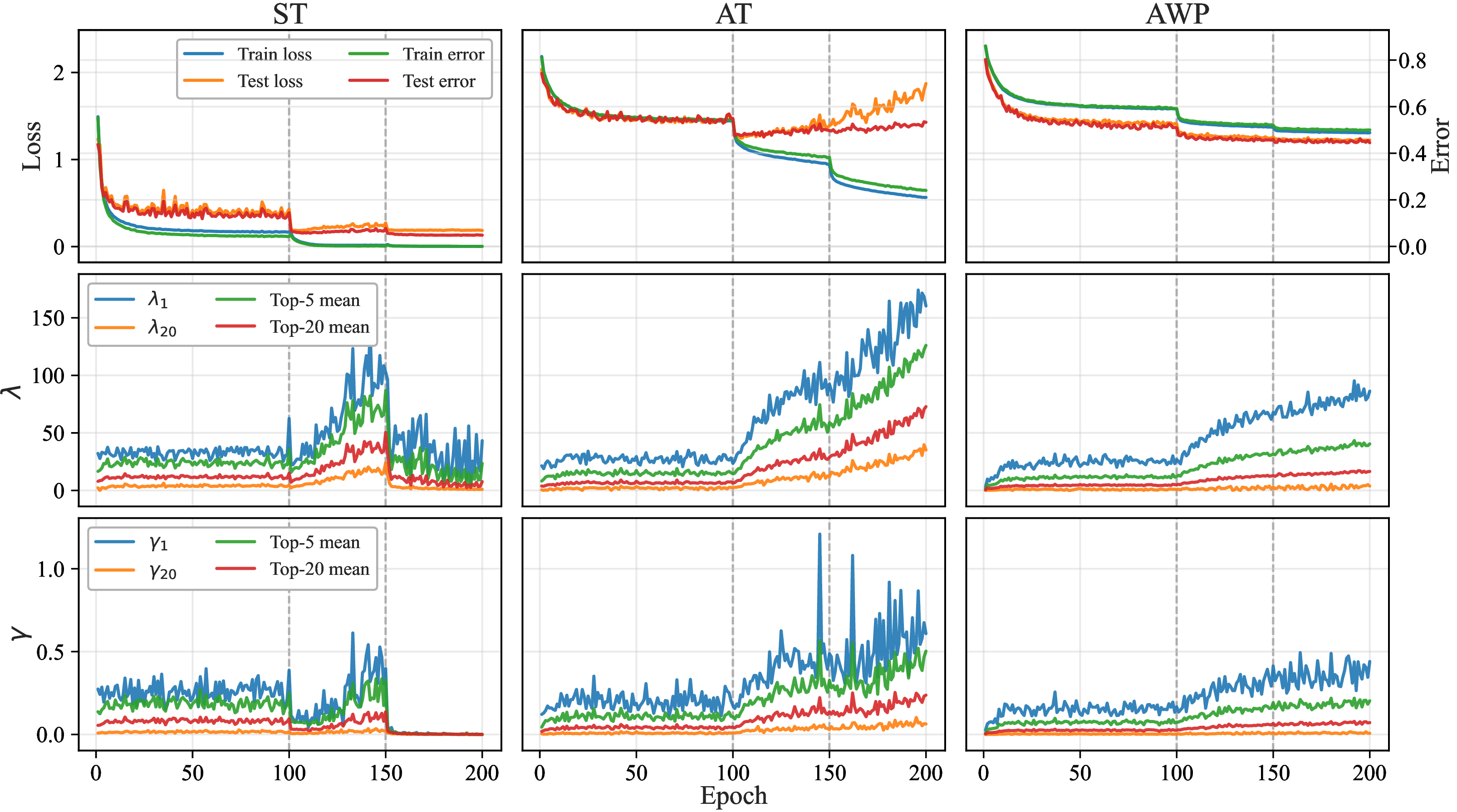
Figure 1 visualizes the learning curves of statistics, including training and testing error/loss, top-\(k\) Hessian eigenvalues \(\{\lambda_i\}_{i=1}^k\), and the corresponding projected gradient-noise variances \(\{\gamma_i\}_{i=1}^k\), across different algorithms (ST, AT, and AWP). Note that the \(i\)-th pair \((\lambda_i, \gamma_i)\) is associated with the \(i\)-th leading eigenvector of the Hessian matrix at the evaluated epoch. We follow the spectral estimation protocol described in Section 5.1 to obtain these estimates. To illustrate the dominating trend while keeping presentation cleanliness, we report the following summary spectral statistics: top-1, top-20, the mean of top-5, and the mean of top-20.

Notably, adversarial training depicts a stage-wise curve separated by the learning rate change. During the initial phase, both the robust loss and error steadily decrease until reaching a plateau, while the top Hessian eigenvalues and gradient noise stay small. After the learning rate decays by a factor of \(10\), both \(\lambda_i\) and \(\gamma_i\) exhibit a monotonically increasing trend, corresponding to a continual decrease in training robust error/loss but steadily worsening test statistics. The final stage is characterized by the smallest \(\eta=0.001\), the top Hessian eigenvalue remaining very large and continuing to increase, and the test robust accuracy dropping further. These observations align with the local stability condition in Section 4.2: top Hessian eigenvalues are capped by \(2(1+\kappa)/\eta\), which is inversely proportional to the learning rate; a large learning rate \(\eta\) will restrict the optimization in low-curvature regions, while reducing \(\eta\) will relax the constraint, allowing the model to move into regions with higher curvature.

In sharp contrast to AT, the learning curves of ST demonstrate a different trend, especially in the final learning stage. Top Hessian eigenvalues are also progressively sharpened when \(\eta=0.01\), indicating the model is gradually fitting more fine-grained features within the training data; however, both \(\lambda_i\) and \(\gamma_i\) suddenly drop to close to zero and remain very low when \(\eta\) drops to \(0.001\). We note that the learning curves of Hessian eigenspectrum match the double descent phenomenon [40], where SGD noise implicitly biases towards flat regions for over-parameterized neural networks. In addition, AWP penalizes the model’s sharpness by perturbing weight parameters, leading to suppressed growth of both \(\lambda_i\) and \(\gamma_i\) in later training stages.

In our experiments, we observe that the top Hessian eigenvalues of adversarially trained models are much higher than those of standard trained models, especially when \(\eta\) is small. This suggests that optimizing adversarial training losses requires exploring high-curvature regions in the parameter space. The following proposition, proven in Appendix 9.2, provides a theoretical justification for the above statement.

Proposition 4 shows that to fit the training data well, robust learning algorithms need to explore high-curvature regions. Unlike ST, it is not possible for adversarial training to learn a model that is “flat” in all directions; a few large Hessian eigenvalues associated with robust features are necessary to ensure the input gradient sensitivity is sufficiently penalized.

5.3 Posterior Collapse & Variance Amplification↩︎

Based on the per-epoch spectral estimates, we can now empirically estimate the posterior mean, posterior covariance, and the bound decompositions in Theorem 3. The full bound contains KL terms beyond the log-determinant proxy, including the mean-norm term and the covariance-trace shift \(\lambda_{t,i}\mapsto \lambda_{t,i}+1/(\beta\sigma_{\mathcal{P}}^2)\) (see Appendix 12.2 for full diagnostics). Specifically, we approximate the spectral estimates using top-\(k\) partial sums with \(k\in\{1,5,10,20\}\) for both the curvature-weighted variance term \(\frac{1}{2}\sum_{i=1}^k\lambda_i\sigma_i^2\) and the entropic KL term \(-\sum_{i=1}^k\ln(\sigma_i^2)\). We use the stationary estimates by default and switch to non-stationary recursion during the transient phase after \(\eta\) decays (Appendix 10.2).

Figure 2 visualizes the learning curves across different algorithms. For AT, we observe that the inferred top-\(k\) posterior covariance contracts sharply after \(\eta\) decays at epochs \(100\) and \(150\), reflected by the stark increase in the entropic KL term and the sharp drop in the variance. This is evident if we derive the closed-form solutions for both terms under the stationary regime and assume commutativity (Lemma 3). Formally, for any \(i=1,2,\ldots,k\), we have \[\begin{align} \lambda_{i}\,\sigma_{i}^2 &= \bigg( 2- \frac{\eta\lambda_i}{1+\kappa}\bigg)^{-1} \frac{\eta}{1-\kappa} \gamma_i, \\ \ln (\sigma_{i}^2) &= \ln \Big(\frac{\eta}{1-\kappa}\Big) + \ln \bigg( \frac{\gamma_i}{\lambda_i} \bigg) - \ln \bigg(2- \frac{\eta\lambda_i}{1+\kappa}\bigg). \end{align}\] Appendix 12.1 provides empirical analysis examining the commutativity assumption, showing that the top Hessian eigendirections largely align with the gradient noise covariance. When \(\eta\) suddenly drops by a factor of \(10\), \(\lambda_i\) and \(\gamma_i\) remain similar, so the immediate change is primarily associated with the drop in \(\eta\). Note that the decrease in \(\lambda_{i}\,\sigma_{i}^2\) is approximately linear in \(\eta\) (dominating factor), whereas the rise in \(-\ln (\sigma_{i}^2)\) is logarithmic in \(\eta\) (less drastic), which explains the initial drop of the testing curves in Figure 1.

As adversarial training continues, the curvature-weighted variance gradually increases, which coincides with increases in \(\lambda_i\) and \(\gamma_i\). In comparison, the entropic KL term remains roughly constant during each stage. Note that, as illustrated in Figure 1, the top Hessian eigenvalues rise by a factor of \(4\) from epoch \(100\) to epoch \(150\) while noise variances increase by a factor of \(2\), jointly boosting the variance at the later stages of adversarial training. The observed trend aligns with the test-robust error curve during the onset of robust overfitting after the learning rate decay, suggesting that it has a dominating influence on robust generalization. Besides, the first- and second-order biases remain at a consistent level throughout training, with only a few large spikes observed at certain epochs. We hypothesize that the spike is due to the (mis-)alignment of input gradients across minibatches.

Compared across the three tested learning algorithms, ST exhibits greater posterior contraction than AT, almost vanishing when \(\eta = 0.001\). Such a collapsing posterior leads to a continuous decrease in curvature-weighted variance. The two bias terms approach zero after the learning rate decays. AWP, on the other hand, penalizes loss curvature, which benefits a more controlled variance and explains why it improves robust generalization. Interestingly, the two bias terms diverge gradually, suggesting that AWP may underfit the training objectives due to excessive penalization. These observations align with AWP’s high training loss observed in Figure 1. Consequently, a promising future direction for our work is to develop a selective penalization scheme for AWP to reduce the training robust loss while preserving its generalization benefits. Combining with the insights from Proposition 6, future designs should balance controlling the curvature-weighted variance to avoid robust overfitting while relaxing regularization strength in directions that capture robust features to enhance the fit of training data.

5.4 Mechanistic Interpretation of Robust Overfitting↩︎

Based on our time-resolved PAC-Bayesian robust generalization bounds and the corresponding empirical diagnostic curves, we can now summarize the underlying mechanisms of robust overfitting. Prior to the first learning-rate drop in adversarial training, the system reaches a stationary state. Due to the stability condition, Hessian eigenvalues are regularized: \(0 < \lambda_i < 2(1+\kappa)/\eta\). However, as illustrated by Proposition 4, lowering adversarial loss requires stabilizing input sensitivity, suggesting the need to explore high-curvature regions to further improve optimization.

After \(\eta\) sharply decays, the system begins to explore high-curvature directions to further reduce the adversarial training loss. Since the system has only evolved gradually at the initial steps, the Hessian and gradient noise covariance remain similar; however, the posterior will rapidly concentrate due to the sharp learning-rate drop (\(\eta \rightarrow \eta/10\)), effectively lowering the curvature-weighted variance \(\frac{1}{2} \sum_{i=1}^m \lambda_{t,i}\,\sigma_{t,i}^2\). While contracted posterior fluctuation also increases the entropic KL-penalty term \(- \frac{1}{2\beta} \sum_{i=1}^m \ln \sigma_{t,i}^2\), it cannot offset the linear decrease in variance. Continual training with a small \(\eta\) keeps increasing Hessian eigenvalues, eventually boosting the variance term and worsening robust generalization. The above mechanistic interpretation matches the empirical observation of robust overfitting well: test robust error first quickly drops after a learning rate decay, then continues to rise, whereas the training loss keeps decreasing.

6 Conclusion↩︎

We derived time-resolved PAC-Bayesian robust generalization bounds by modeling momentum SGD as a discrete-time dynamical system and deriving closed-form posterior evolutions that depend on the learning rate, the loss geometry, and the stochastic gradient noise. Through theoretical analysis, empirical diagnostics, and controlled experiments, our work provides mechanistic insights into how learning dynamics lead to robust overfitting or generalization. Looking forward, important directions include extending our framework to more general settings, such as adaptive optimizers and relaxed assumptions, and leveraging the insights to enhance the training-time fit of AWP while avoiding overfitting.

Availability↩︎

The code for implementing our spectral estimation algorithm and reproducing our main experimental results is available at: https://github.com/TrustMLRG/RobustGen.

7 Proofs of Theoretical Results in Section 4.1↩︎

7.1 Proof of Lemma 1↩︎

According to the definition of KL divergence, we have \[\begin{align} \label{eq:general32KL32divergence32def} \mathrm{KL}\!\left(\mathcal{Q}\,\|\,\mathcal{P}\right) = \int q(\boldsymbol{w}) \,\ln \frac{q(\boldsymbol{w})}{p(\boldsymbol{w})}\,\mathrm{d}\boldsymbol{w} = \mathbb{E}_{\boldsymbol{w}\sim\mathcal{Q}}\!\left[\ln q(\boldsymbol{w}) - \ln p(\boldsymbol{w})\right], \end{align}\tag{17}\] where the density functions of \(\mathcal{P}\) and \(\mathcal{Q}\) under our assumptions can be written as: \[\begin{align} p(\boldsymbol{w}) &= (2\pi)^{-\frac{m}{2}}\,\sigma_{\mathcal{P}}^{-m} \cdot \exp\!\left(-\frac{1}{2\sigma_{\mathcal{P}}^{2}}\,\boldsymbol{w}^{\!\top}\boldsymbol{w}\right), \\ q(\boldsymbol{w}) &= (2\pi)^{-\frac{m}{2}}\,\det(\mathbf{\Sigma}_{\mathcal{Q}})^{-\frac{1}{2}} \cdot \exp\!\left(-\frac{1}{2}(\boldsymbol{w}-\boldsymbol{\mu}_{\mathcal{Q}})^{\!\top} \mathbf{\Sigma}_{\mathcal{Q}}^{-1}(\boldsymbol{w}-\boldsymbol{\mu}_{\mathcal{Q}})\right). \end{align}\] Taking logs of the above equations, we obtain \[\label{eq:prior32posterior32density32def} \begin{align} \ln p(\boldsymbol{w}) &= -\frac{m}{2}\ln(2\pi) - m\ln\sigma_{\mathcal{P}} -\frac{1}{2\sigma_{\mathcal{P}}^{2}}\,\boldsymbol{w}^{\!\top}\boldsymbol{w}, \\ \ln q(\boldsymbol{w}) &= -\frac{m}{2}\ln(2\pi) - \frac{1}{2}\ln\det(\mathbf{\Sigma}_{\mathcal{Q}}) -\frac{1}{2}(\boldsymbol{w}-\boldsymbol{\mu}_{\mathcal{Q}})^{\!\top}\mathbf{\Sigma}_{\mathcal{Q}}^{-1}(\boldsymbol{w}-\boldsymbol{\mu}_{\mathcal{Q}}). \end{align}\tag{18}\] Plugging Equation 18 into Equation 17 , we further obtain \[\begin{align} \mathrm{KL}\!\left(\mathcal{Q}\,\|\,\mathcal{P}\right) &= \mathbb{E}_{\boldsymbol{w}\sim\mathcal{Q}}\!\Bigg[ -\frac{1}{2}\ln\det(\mathbf{\Sigma}_{\mathcal{Q}}) -\frac{1}{2}(\boldsymbol{w}-\boldsymbol{\mu}_{\mathcal{Q}})^{\!\top}\mathbf{\Sigma}_{\mathcal{Q}}^{-1}(\boldsymbol{w}-\boldsymbol{\mu}_{\mathcal{Q}}) + m\ln\sigma_{\mathcal{P}} + \frac{1}{2\sigma_{\mathcal{P}}^{2}}\,\boldsymbol{w}^{\!\top}\boldsymbol{w} \Bigg] \\ & = -\frac{1}{2}\ln\det(\mathbf{\Sigma}_{\mathcal{Q}}) -\frac{m}{2} + m\ln\sigma_{\mathcal{P}} +\frac{1}{2\sigma_{\mathcal{P}}^{2}}\!\left(\mathrm{Tr}(\mathbf{\Sigma}_{\mathcal{Q}}) + \|\boldsymbol{\mu}_{\mathcal{Q}}\|_{2}^{2}\right), \end{align}\] where the last equality holds because \(\mathcal{Q} = \mathcal{N}(\boldsymbol{\mu}_{\mathcal{Q}}, \mathbf{\Sigma}_{\mathcal{Q}})\). Specifically, for any \(\boldsymbol{w}\sim\mathcal{Q}\), \(\mathbf{\Sigma}^{-1/2}(\boldsymbol{w} - \boldsymbol{\mu}_{\mathcal{Q}}) \sim \mathcal{N}(\boldsymbol{0}, \mathbf{I})\), which suggests that \(\mathbb{E}_{\mathcal{Q}}\!\left[(\boldsymbol{w}-\boldsymbol{\mu}_{\mathcal{Q}})^{\!\top}\mathbf{\Sigma}_{\mathcal{Q}}^{-1}(\boldsymbol{w}-\boldsymbol{\mu}_{\mathcal{Q}})\right] = m\), and \(\mathbb{E}_{\mathcal{Q}}\!\left[\boldsymbol{w}^{\!\top}\boldsymbol{w}\right] = \mathbb{E}_{\mathcal{Q}}\!\left[\|\boldsymbol{w}-\boldsymbol{\mu}_{\mathcal{Q}}\|_2^2\right] + \|\boldsymbol{\mu}_{\mathcal{Q}}\|_2^2 = \mathrm{Tr}(\mathbf{\Sigma_{\mathcal{Q}}}) + \|\boldsymbol{\mu}_{\mathcal{Q}}\|_2^2\). Therefore, we complete the proof of Lemma 1.

7.2 Proof of Lemma 2↩︎

Under the local quadratic upper-bound assumption in Lemma 2, the empirical adversarial loss satisfies the following Taylor upper expansion around the reference point \(\tilde{\boldsymbol{w}}\): \[\label{eq:quad-form} \hat{\mathcal{L}}_{\epsilon}(\boldsymbol{w}) \le \hat{\mathcal{L}}_{\epsilon}(\tilde{\boldsymbol{w}}) + \nabla \hat{\mathcal{L}}_{\epsilon}(\tilde{\boldsymbol{w}})^\top (\boldsymbol{w} - \tilde{\boldsymbol{w}}) +\frac{1}{2}\,(\boldsymbol{w}-\tilde{\boldsymbol{w}})^{\!\top}\hat{\mathbf{H}}_{\epsilon}(\tilde{\boldsymbol{w}})(\boldsymbol{w}-\tilde{\boldsymbol{w}}) +r_{\tilde{\boldsymbol{w}}}(\boldsymbol{w}), \text{ for any } \boldsymbol{w}\sim\mathcal{Q},\tag{19}\] where \(\nabla \hat{\mathcal{L}}_{\epsilon}(\tilde{\boldsymbol{w}})\) (resp. \(\hat{\mathbf{H}}_{\epsilon}(\tilde{\boldsymbol{w}})\)) denotes the gradient (resp. Hessian) of the empirical adversarial loss at the reference point.

Taking expectation over \(\boldsymbol{w}\sim\mathcal{Q}=\mathcal{N}(\boldsymbol{\mu}_{\mathcal{Q}},\mathbf{\Sigma}_{\mathcal{Q}})\), we have \[\begin{align} \label{eq:second32order32taylor32expansion32Lemma324462} \mathbb{E}_{\boldsymbol{w}\sim\mathcal{Q}}\!\left[\hat{\mathcal{L}}_{\epsilon}(\boldsymbol{w})\right] \le\;&\hat{\mathcal{L}}_{\epsilon}(\tilde{\boldsymbol{w}}) + \nabla \hat{\mathcal{L}}_{\epsilon}(\tilde{\boldsymbol{w}})^\top \mathbb{E}_{\boldsymbol{w}\sim\mathcal{Q}}[(\boldsymbol{w} - \tilde{\boldsymbol{w}})] \nonumber\\ &+\frac{1}{2}\,\mathbb{E}_{\boldsymbol{w}\sim\mathcal{Q}}\!\left[(\boldsymbol{w}-\tilde{\boldsymbol{w}})^{\!\top}\hat{\mathbf{H}}_{\epsilon}(\tilde{\boldsymbol{w}})(\boldsymbol{w}-\tilde{\boldsymbol{w}})\right] + \mathbb{E}_{\boldsymbol{w}\sim\mathcal{Q}}[r_{\tilde{\boldsymbol{w}}}(\boldsymbol{w})]. \end{align}\tag{20}\] Let \(\Delta \bar{\boldsymbol{w}} := \boldsymbol{\mu}_{\mathcal{Q}} - \tilde{\boldsymbol{w}}\) denote the posterior mean shift. Since \(\mathbb{E}_{\boldsymbol{w}\sim\mathcal{Q}}[\boldsymbol{w}] = \boldsymbol{\mu}_{\mathcal{Q}}\), we have \[\begin{align} \label{eq:linear32term32Lemma324462} \mathbb{E}_{\boldsymbol{w}\sim\mathcal{Q}}[(\boldsymbol{w} - \tilde{\boldsymbol{w}})] = \boldsymbol{\mu}_{\mathcal{Q}} - \tilde{\boldsymbol{w}} = \Delta \bar{\boldsymbol{w}}. \end{align}\tag{21}\] The remaining task is to simplify the quadratic term in Equation 20 . From the second-moment identity, we know \[\begin{align} \label{eq:basic32quadratic32term32Lemma324462} \mathbb{E}_{\boldsymbol{w}\sim\mathcal{Q}}\!\left[(\boldsymbol{w}-\tilde{\boldsymbol{w}})(\boldsymbol{w}-\tilde{\boldsymbol{w}})^{\!\top}\right] =\mathbf{\Sigma}_{\mathcal{Q}}+\Delta \bar{\boldsymbol{w}}\,{\Delta \bar{\boldsymbol{w}}}^{\!\top}, \end{align}\tag{22}\] which holds for any Gaussian with mean \(\boldsymbol{\mu}_{\mathcal{Q}}\) and covariance \(\mathbf{\Sigma}_{\mathcal{Q}}\). Hence, we have \[\begin{align} \label{eq:quadratic32term32Lemma324462} \nonumber \mathbb{E}_{\boldsymbol{w}\sim\mathcal{Q}}\!\left[(\boldsymbol{w}-\tilde{\boldsymbol{w}})^{\!\top}\hat{\mathbf{H}}_{\epsilon}(\tilde{\boldsymbol{w}})(\boldsymbol{w}-\tilde{\boldsymbol{w}})\right] &= \mathbb{E}_{\boldsymbol{w}\sim\mathcal{Q}} \left[ \mathrm{Tr}\!\left( (\boldsymbol{w}-\tilde{\boldsymbol{w}})^{\top} \hat{\mathbf{H}}_{\epsilon}(\tilde{\boldsymbol{w}}) (\boldsymbol{w}-\tilde{\boldsymbol{w}}) \right) \right] \\ \nonumber &= \mathrm{Tr}\!\left(\hat{\mathbf{H}}_{\epsilon}(\tilde{\boldsymbol{w}})\,\mathbb{E}\!\left[(\boldsymbol{w}-\tilde{\boldsymbol{w}})(\boldsymbol{w}-\tilde{\boldsymbol{w}})^{\!\top}\right]\right) \\ \nonumber &= \mathrm{Tr}\!\left(\hat{\mathbf{H}}_{\epsilon}(\tilde{\boldsymbol{w}})\mathbf{\Sigma}_{\mathcal{Q}}\right) + \mathrm{Tr}\!\left(\hat{\mathbf{H}}_{\epsilon}(\tilde{\boldsymbol{w}})\Delta \bar{\boldsymbol{w}}\,{\Delta \bar{\boldsymbol{w}}}^{\!\top}\right) \\ &= \mathrm{Tr}\!\left(\hat{\mathbf{H}}_{\epsilon}(\tilde{\boldsymbol{w}})\mathbf{\Sigma}_{\mathcal{Q}}\right) + {\Delta \bar{\boldsymbol{w}}}^{\!\top}\hat{\mathbf{H}}_{\epsilon}(\tilde{\boldsymbol{w}})\Delta \bar{\boldsymbol{w}}, \end{align}\tag{23}\] where the second and the last equalities hold because of the cyclic property of trace: \(\mathrm{Tr}(\mathbf{A}\mathbf{u}\mathbf{u}^{\!\top}) = \mathrm{Tr}(\mathbf{u}^{\!\top}\mathbf{A}\mathbf{u})\) holds for any matrix \(\mathbf{A}\) and vector \(\boldsymbol{u}\), and the third equality is due to Equation 22 .

Plugging Equation 21 and Equation 23 into Equation 20 yields \[\mathbb{E}_{\boldsymbol{w}\sim\mathcal{Q}} \big[ \hat{\mathcal{L}}_{\epsilon}(\boldsymbol{w}) \big] \le \hat{\mathcal{L}}_{\epsilon}(\tilde{\boldsymbol{w}}) + \nabla \hat{\mathcal{L}}_{\epsilon}(\tilde{\boldsymbol{w}})^\top \Delta \bar{\boldsymbol{w}} + \frac{1}{2} {\Delta \bar{\boldsymbol{w}}}^{\top} \hat{\mathbf{H}}_{\epsilon}(\tilde{\boldsymbol{w}}) \Delta \bar{\boldsymbol{w}} + \frac{1}{2} \mathrm{Tr}(\hat{\mathbf{H}}_{\epsilon}(\tilde{\boldsymbol{w}}) \mathbf{\Sigma}_{\mathcal{Q}}) + R_{\mathcal{Q}}(\tilde{\boldsymbol{w}}),\] where \(R_{\mathcal{Q}}(\tilde{\boldsymbol{w}})=\mathbb{E}_{\boldsymbol{w}\sim\mathcal{Q}}[r_{\tilde{\boldsymbol{w}}}(\boldsymbol{w})]\). This completes the proof of Lemma 2.

7.3 Proof of Theorem 2↩︎

We start from the generic PAC-Bayesian robust generalization bound in Theorem 1: \[\begin{align} \label{eq:appendix95compact95bound95start} \mathbb{E}_{\boldsymbol{w} \sim \mathcal{Q}} \big[ \mathcal{L}_{\epsilon}(\boldsymbol{w}) \big] \le \mathbb{E}_{\boldsymbol{w} \sim \mathcal{Q}} \big[ \hat{\mathcal{L}}_{\epsilon}(\boldsymbol{w}) \big] + \frac{1}{\beta} \mathrm{KL}(\mathcal{Q} \,\|\, \mathcal{P}) + \frac{\beta C_\ell^{2}}{8 |\mathcal{S}|} - \frac{1}{\beta} \ln{\alpha}. \end{align}\tag{24}\]

Step 1: Expected empirical adversarial loss under a Gaussian posterior. Under the local quadratic upper bound of Lemma 2, we have \[\begin{align} \label{eq:appendix95compact95empirical} \mathbb{E}_{\boldsymbol{w}\sim\mathcal{Q}} \big[\hat{\mathcal{L}}_{\epsilon}(\boldsymbol{w})\big] &\le \hat{\mathcal{L}}_{\epsilon}(\tilde{\boldsymbol{w}}) + \big\langle \nabla \hat{\mathcal{L}}_{\epsilon}(\tilde{\boldsymbol{w}}), \Delta \bar{\boldsymbol{w}} \big\rangle + \frac{1}{2} {\Delta \bar{\boldsymbol{w}}}^{\top} \hat{\mathbf{H}}_{\epsilon} (\tilde{\boldsymbol{w}}) \Delta \bar{\boldsymbol{w}} + \frac{1}{2} \mathrm{Tr} \big( \hat{\mathbf{H}}_{\epsilon}(\tilde{\boldsymbol{w}}) \mathbf{\Sigma}_{\mathcal{Q}} \big) +R_{\mathcal{Q}}(\tilde{\boldsymbol{w}}), \end{align}\tag{25}\] where \(\Delta \bar{\boldsymbol{w}}=\boldsymbol{\mu}_{\mathcal{Q}}-\tilde{\boldsymbol{w}}\).

Step 2: Closed-form KL divergence. For the spherical Gaussian prior \(\mathcal{P}=\mathcal{N}(\boldsymbol{0},\sigma_{\mathcal{P}}^{2}\mathbf{I})\) and Gaussian posterior \(\mathcal{Q}=\mathcal{N}(\boldsymbol{\mu}_{\mathcal{Q}},\mathbf{\Sigma}_{\mathcal{Q}})\), Lemma 1 yields \[\begin{align} \label{eq:appendix95compact95kl} \frac{1}{\beta}\mathrm{KL}(\mathcal{Q}\,\|\,\mathcal{P}) &= \underbrace{ \frac{1}{2\beta \sigma^{2}_{\mathcal{P}}} \Big(\| \boldsymbol{\mu}_{\mathcal{Q}} \|_{2}^{2} + \mathrm{Tr}(\mathbf{\Sigma}_{\mathcal{Q}})\Big) - \frac{1}{2\beta} \ln \det (\mathbf{\Sigma}_{\mathcal{Q}}) }_{\text{terms depending on }\mathcal{Q}} + \underbrace{\frac{m}{2\beta}\ln(\sigma^2_{\mathcal{P}}) - \frac{m}{2\beta}}_{\text{constant in }\mathcal{Q}} . \end{align}\tag{26}\]

Step 3: Combine terms. Substituting equation 25 and equation 26 into equation 24 , and grouping all terms independent of the posterior \(\mathcal{Q}\) into \[\begin{align} \label{eq:Pac32Bayes32remainder32term} C_{\mathrm{PB}} = C_{\mathrm{PB}}(\sigma^2_{\mathcal{P}}, \mathcal{S}, \alpha, \beta) = \frac{m}{2\beta}\ln\sigma^2_{\mathcal{P}} - \frac{m}{2\beta} + \frac{\beta C_\ell^2}{8|\mathcal{S}|} - \frac{1}{\beta}\ln\alpha, \end{align}\tag{27}\] where we obtain exactly the bound in Equation 10 , including the local Taylor upper remainder.

7.4 Robust Generalization Bounds under Gaussian-Mixture Posterior↩︎

We start with the most general PAC-Bayesian bound in Theorem 1, since it holds for any posterior \(\mathcal{Q}\). For any \(\beta>0\) and any \(\alpha\in(0,1)\), with probability at least \(1-\alpha\) over the finite sample set \(\mathcal{S}\), we have \[\begin{align} \label{eq:appendix95mixture95catoni95start} \mathbb{E}_{\boldsymbol{w}\sim\mathcal{Q}}[\mathcal{L}_{\epsilon}(\boldsymbol{w})] \leq \mathbb{E}_{\boldsymbol{w}\sim\mathcal{Q}} \bigg[ \frac{1}{|\mathcal{S}|} \sum_{(\boldsymbol{x},y)\in\mathcal{S}} \ell_{\mathrm{adv}}(\boldsymbol{w},\boldsymbol{x},y) \bigg] + \frac{1}{\beta}\mathrm{KL}(\mathcal{Q}\,\|\,\mathcal{P}) + \frac{\beta C_\ell^{2}}{8|\mathcal{S}|} - \frac{1}{\beta}\ln\alpha . \end{align}\tag{29}\] We now instantiate this bound by choosing the posterior to be a mixture of Gaussian distributions specified in Equation 28 and the prior \(\mathcal{P}=\mathcal{N}(0,\sigma_{\mathcal{P}}^{2}\mathbf{I})\).

Step 1: Decomposition of the empirical adversarial loss. By the definition of expectations under mixture distributions, for any measurable function \(f:\mathcal{W}\to\mathbb{R}\), \[\begin{align} \label{eq:appendix95mixture95expectation95identity} \mathbb{E}_{\boldsymbol{w}\sim\mathcal{Q}}[f(\boldsymbol{w})] = \sum_{\ell=1}^{L} \pi_{\ell} \, \mathbb{E}_{\boldsymbol{w}\sim\mathcal{Q}_{\ell}}[f(\boldsymbol{w})]. \end{align}\tag{30}\] Applying Equation 30 to \(f(\boldsymbol{w}) = \hat{\mathcal{L}}_{\epsilon}(\boldsymbol{w})\) gives \[\begin{align} \label{eq:appendix95mixture95empirical95decomp} \mathbb{E}_{\boldsymbol{w}\sim\mathcal{Q}} \big[\hat{\mathcal{L}}_{\epsilon}(\boldsymbol{w})\big] = \sum_{\ell=1}^{L} \pi_{\ell}\, \mathbb{E}_{\boldsymbol{w}\sim\mathcal{Q}_{\ell}} \big[\hat{\mathcal{L}}_{\epsilon}(\boldsymbol{w})\big]. \end{align}\tag{31}\] For each Gaussian component \(\mathcal{Q}_{\ell}\), note that we assume \(\hat{\mathcal{L}}_{\epsilon}(\boldsymbol{w})\) can be locally upper bounded around the basin-specific reference point \(\boldsymbol{w}_{\text{ref},\ell}\) by a quadratic form with Hessian \(\mathbf{H}_{\ell}\) and gradient \(\boldsymbol{g}_{\ell}:=\nabla \hat{\mathcal{L}}_{\epsilon}(\boldsymbol{w}_{\text{ref},\ell})\). Thus, applying Lemma 2 to each component, we obtain \[\begin{align} \label{eq:appendix95mixture95empirical95component} \mathbb{E}_{\boldsymbol{w}\sim\mathcal{Q}_{\ell}} \big[\hat{\mathcal{L}}_{\epsilon}(\boldsymbol{w})\big] \le \hat{\mathcal{L}}_{\epsilon}(\boldsymbol{w}_{\text{ref},\ell}) + \boldsymbol{g}_{\ell}^\top(\boldsymbol{\mu}_{\ell}-\boldsymbol{w}_{\text{ref},\ell}) + \frac{1}{2} (\boldsymbol{\mu}_{\ell}-\boldsymbol{w}_{\text{ref},\ell})^\top \mathbf{H}_{\ell} (\boldsymbol{\mu}_{\ell}-\boldsymbol{w}_{\text{ref},\ell}) + \frac{1}{2} \mathrm{Tr}(\mathbf{H}_{\ell}\mathbf{\Sigma}_{\ell}) + R_{\mathcal{Q}_{\ell}}(\boldsymbol{w}_{\text{ref},\ell}). \end{align}\tag{32}\]

Substituting Equation 32 into Equation 31 yields the mixture-expanded empirical loss: \[\begin{align} \label{eq:appendix95mixture95empirical95final} \nonumber \mathbb{E}_{\boldsymbol{w}\sim\mathcal{Q}} [\hat{\mathcal{L}}_{\epsilon}(\boldsymbol{w})] &\le \sum_{\ell=1}^{L} \pi_{\ell} \Big[ \hat{\mathcal{L}}_{\epsilon}(\boldsymbol{w}_{\text{ref},\ell}) +\boldsymbol{g}_{\ell}^\top(\boldsymbol{\mu}_{\ell}-\boldsymbol{w}_{\text{ref},\ell}) \\ &\qquad +\frac{1}{2}(\boldsymbol{\mu}_{\ell}-\boldsymbol{w}_{\text{ref},\ell})^\top \mathbf{H}_{\ell} (\boldsymbol{\mu}_{\ell}-\boldsymbol{w}_{\text{ref},\ell}) +\frac{1}{2}\mathrm{Tr}(\mathbf{H}_{\ell}\mathbf{\Sigma}_{\ell}) +R_{\mathcal{Q}_{\ell}}(\boldsymbol{w}_{\text{ref},\ell}) \Big]. \end{align}\tag{33}\]

Step 2: KL divergence upper bound for the mixture posterior. Since KL divergence is convex in its first argument, the mixture posterior \(\mathcal{Q}=\sum_{\ell=1}^{L}\pi_{\ell}\mathcal{Q}_{\ell}\) satisfies \[\begin{align} \label{eq:appendix95mixture95kl95convexity} \mathrm{KL}(\mathcal{Q}\,\|\,\mathcal{P}) = \mathrm{KL}\Big(\sum_{\ell=1}^{L}\pi_{\ell}\mathcal{Q}_{\ell}\,\Big\|\,\mathcal{P}\Big) \leq \sum_{\ell=1}^{L} \pi_{\ell}\, \mathrm{KL}(\mathcal{Q}_{\ell}\,\|\,\mathcal{P}), \end{align}\tag{34}\] where the inequality follows from the definition KL divergence and the log sum inequality. For each \(\mathcal{Q}_{\ell}=\mathcal{N}(\boldsymbol{\mu}_{\ell},\mathbf{\Sigma}_{\ell})\), Lemma 1 provides the closed-form expression: \[\begin{align} \label{eq:appendix95mixture95kl95component} \mathrm{KL}(\mathcal{Q}_{\ell}\,\|\,\mathcal{P}) = \frac{\mathrm{Tr}(\mathbf{\Sigma}_{\ell})}{2\sigma_{\mathcal{P}}^{2}} +\frac{\|\boldsymbol{\mu}_{\ell}\|_{2}^{2}}{2\sigma_{\mathcal{P}}^{2}} -\frac{m}{2} +\frac{m}{2}\ln\sigma_{\mathcal{P}}^{2} -\frac{1}{2}\ln\det\mathbf{\Sigma}_{\ell}. \end{align}\tag{35}\]

Multiplying Equation 34 by \(1/\beta\) and substituting Equation 35 yields \[\begin{align} \label{eq:appendix95mixture95kl95final} \frac{1}{\beta}\mathrm{KL}(\mathcal{Q}\,\|\,\mathcal{P}) \leq \sum_{\ell=1}^{L} \frac{\pi_{\ell}}{2\beta} \left( \frac{\mathrm{Tr}(\mathbf{\Sigma}_{\ell})}{\sigma_{\mathcal{P}}^{2}} +\frac{\|\boldsymbol{\mu}_{\ell}\|_{2}^{2}}{\sigma_{\mathcal{P}}^{2}} -m +m\ln\sigma_{\mathcal{P}}^{2} -\ln\det\mathbf{\Sigma}_{\ell} \right). \end{align}\tag{36}\]

Finally, we substitute the empirical-loss expansion (Equation 33 ) and the KL bound (Equation 36 ) into Equation 29 . Noticing that the remaining terms, where \(C_\ell\) denotes the global scalar loss-bound constant, \(\frac{\beta C_\ell^{2}}{8|\mathcal{S}|}\) and \(-\frac{1}{\beta}\ln(\alpha)\) do not depend on the mixture-component index \(\ell\), we obtain \[\mathbb{E}_{\boldsymbol{w}\sim\mathcal{Q}}[\mathcal{L}_{\epsilon}(\boldsymbol{w})] \leq \sum_{\ell=1}^{L} \pi_{\ell} \Big[ \hat{\mathcal{L}}_{\epsilon}(\boldsymbol{w}_{\text{ref},\ell}) +\boldsymbol{g}_{\ell}^\top(\boldsymbol{\mu}_{\ell}-\boldsymbol{w}_{\text{ref},\ell}) +\frac{1}{2}(\boldsymbol{\mu}_{\ell}-\boldsymbol{w}_{\text{ref},\ell})^\top \mathbf{H}_{\ell}(\boldsymbol{\mu}_{\ell}-\boldsymbol{w}_{\text{ref},\ell}) +\frac{1}{2}\mathrm{Tr}(\mathbf{H}_{\ell}\mathbf{\Sigma}_{\ell}) +R_{\mathcal{Q}_{\ell}}(\boldsymbol{w}_{\text{ref},\ell}) \Big]\] \[\hphantom{\mathbb{E}_{\boldsymbol{w}\sim\mathcal{Q}}[\mathcal{L}_{\epsilon}(\boldsymbol{w})]} +\; \sum_{\ell=1}^{L} \frac{\pi_{\ell}}{2\beta} \left( \frac{\mathrm{Tr}(\mathbf{\Sigma}_{\ell})}{\sigma_{\mathcal{P}}^{2}} +\frac{\|\boldsymbol{\mu}_{\ell}\|_{2}^{2}}{\sigma_{\mathcal{P}}^{2}} -m +m\ln\sigma_{\mathcal{P}}^{2} -\ln\det\mathbf{\Sigma}_{\ell} \right) +\frac{\beta C_\ell^{2}}{8|\mathcal{S}|} -\frac{1}{\beta}\ln\alpha.\]

This expression gives the stated upper bound in Corollary 1, completing the proof.

8 Proofs of Theoretical Results in Section 4.2↩︎

8.1 Stationary Regime: Proof of Lemma 3↩︎

Under the generalized quadratic loss approximation, the stochastic gradient includes a constant drift \(\boldsymbol{g}_{\text{ref}}:= \nabla \hat{\mathcal{L}}_{\epsilon}(\boldsymbol{w}_{\text{ref}})\). For covariance calculations, we can omit this term without loss of generality, because covariance measures centered fluctuations: letting \(\tilde{\boldsymbol{u}}_t = \boldsymbol{u}_t - \mathbb{E}[\boldsymbol{u}_t]\) denote the centered state, the drift appears identically in both \(\boldsymbol{u}_t\) and \(\mathbb{E}[\boldsymbol{u}_t]\) and cancels upon subtraction. This cancellation holds regardless of whether the system is stationary or transient (the multi-step transient recursion is handled in the proof of Lemma 4).

Throughout this proof, we treat the training set \(\mathcal{S}\) (and hence the empirical loss \(\hat{\mathcal{L}}_{\epsilon}\)) as fixed, and take all expectations/covariances with respect to the algorithmic randomness conditional on \(\mathcal{S}\).

State-space form. To begin with, we prove Equation 11 . From the updates in Equation 4 , we have \[\begin{align} \boldsymbol{v}_{t+1} &= \kappa\,\boldsymbol{v}_{t} + \boldsymbol{g}_{\text{ref}} + \mathbf{H}_{\text{ref}}(\boldsymbol{w}_{t}-\boldsymbol{w}_{\text{ref}}) + \boldsymbol{\xi}_{t},\\ \boldsymbol{w}_{t+1}-\boldsymbol{w}_{\text{ref}} &= (\boldsymbol{w}_{t}-\boldsymbol{w}_{\text{ref}}) - \eta \boldsymbol{v}_{t+1} = (\mathbf{I} - \eta \mathbf{H}_{\text{ref}})(\boldsymbol{w}_{t}-\boldsymbol{w}_{\text{ref}}) - \eta \kappa\,\boldsymbol{v}_{t} - \eta\,\boldsymbol{g}_{\text{ref}} - \eta\,\boldsymbol{\xi}_{t}. \end{align}\] Stacking the two lines with the joint state \(\boldsymbol{u}_t:=\begin{bmatrix}\boldsymbol{w}_t-\boldsymbol{w}_{\text{ref}}\\ \boldsymbol{v}_t\end{bmatrix}\in\mathbb{R}^{2m}\), we obtain the affine state-space system \[\boldsymbol{u}_{t+1} \;=\; \mathbf{A}\,\boldsymbol{u}_{t} + \mathbf{G}\,\big[\boldsymbol{g}_{\text{ref}}+\boldsymbol{\xi}_{t}\big], \quad \mathbf{A} = \begin{bmatrix} \mathbf{I} - \eta \mathbf{H}_{\text{ref}} & -\eta\kappa\,\mathbf{I} \\ \mathbf{H}_{\text{ref}} & \kappa\,\mathbf{I} \end{bmatrix}, \quad \mathbf{G}=\begin{bmatrix}-\eta\mathbf{I}\\ \mathbf{I}\end{bmatrix},\] which is exactly equation 11 .

Stationary Mean & Covariance. Next, we derive the stationary posterior mean and covariance as in Equations 12 and 13 .

Under the local quadratic approximation in Lemma 2, the gradient of the empirical adversarial loss at any point \(\boldsymbol{w}\) can be written as: \[\nabla_{\boldsymbol{w}} \hat{\mathcal{L}}_{\epsilon}(\boldsymbol{w}) = \nabla \hat{\mathcal{L}}_{\epsilon}(\boldsymbol{w}_{\text{ref}}) + \mathbf{H}_{\text{ref}} (\boldsymbol{w} - \boldsymbol{w}_{\text{ref}}),\] where \(\nabla \hat{\mathcal{L}}_{\epsilon}(\boldsymbol{w}_{\text{ref}}) =: \boldsymbol{g}_{\text{ref}}\) is the (possibly non-zero) gradient at the reference point \(\boldsymbol{w}_{\text{ref}}\).

Taking expectation over the posterior \(\mathcal{Q} = \mathcal{N}(\boldsymbol{\mu}_{\mathcal{Q}}, \mathbf{\Sigma}_{\mathcal{Q}})\), we obtain \[\begin{align} \label{eq:expectation32over32gradient} \mathbb{E}_{\boldsymbol{w}\sim\mathcal{Q}} \big[ \nabla_{\boldsymbol{w}} \hat{\mathcal{L}}_{\epsilon}(\boldsymbol{w}) \big] = \boldsymbol{g}_{\text{ref}} + \mathbf{H}_{\text{ref}} (\boldsymbol{\mu}_{\mathcal{Q}} - \boldsymbol{w}_{\text{ref}}). \end{align}\tag{38}\]

Since the posterior \(\mathcal{Q}\) is stationary and obtained via SGD on \(\hat{\mathcal{L}}_{\epsilon}(\boldsymbol{w})\), the expected gradient must vanish at stationarity. Otherwise, running another step of SGD would shift the mean and break the stationary assumption. Thus, \[\mathbb{E}_{\boldsymbol{w}\sim\mathcal{Q}} \big[ \nabla_{\boldsymbol{w}} \hat{\mathcal{L}}_{\epsilon}(\boldsymbol{w}) \big] = \boldsymbol{0}.\]

Combining with Equation 38 , we have \[\boldsymbol{g}_{\text{ref}} + \mathbf{H}_{\text{ref}} (\boldsymbol{\mu}_{\mathcal{Q}} - \boldsymbol{w}_{\text{ref}}) = \boldsymbol{0}.\]

By the positive-definiteness assumption in Lemma 3, \(\mathbf{H}_{\text{ref}}\succ0\), and hence \(\mathbf{H}_{\text{ref}}\) is invertible. Solving for \(\boldsymbol{\mu}_{\mathcal{Q}}\) yields \[\boldsymbol{\mu}_{\mathcal{Q}} = \boldsymbol{w}_{\text{ref}} - \mathbf{H}_{\text{ref}}^{-1} \nabla \hat{\mathcal{L}}_{\epsilon}(\boldsymbol{w}_{\text{ref}}),\] which matches Equation 12 after identifying \(\boldsymbol{w}_{\text{ref}}\) with \(\tilde{\boldsymbol{w}}\) and \(\mathbf{H}_{\text{ref}}\) with \(\hat{\mathbf{H}}_{\epsilon}(\tilde{\boldsymbol{w}})\). This stationary mean relation has the form of a Newton-type correction around the reference point.

Joint Lyapunov equation and projection. From Lemma 3, the stacked state \(\boldsymbol{u}_t=\begin{bmatrix}\boldsymbol{w}_t-\boldsymbol{w}_{\text{ref}}\\ \boldsymbol{v}_t\end{bmatrix}\in\mathbb{R}^{2m}\) obeys the affine recursion \[\boldsymbol{u}_{t+1}=\mathbf{A}\,\boldsymbol{u}_{t}+\mathbf{G}\big(\boldsymbol{g}_{\text{ref}}+\boldsymbol{\xi}_{t}\big), \qquad \mathbf{A}= \begin{bmatrix} \mathbf{I}-\eta\mathbf{H}_{\text{ref}} & -\eta\kappa\,\mathbf{I}\\ \mathbf{H}_{\text{ref}} & \kappa\,\mathbf{I} \end{bmatrix},\qquad \mathbf{G}=\begin{bmatrix}-\eta\mathbf{I}\\ \mathbf{I}\end{bmatrix}.\] Since covariance is translation-invariant, the drift \(\boldsymbol{g}_{\text{ref}}\) does not affect it: defining the centered state \(\tilde{\boldsymbol{u}}_t:=\boldsymbol{u}_t-\mathbb{E}[\boldsymbol{u}_t\mid\mathcal{S}]\), we have \(\tilde{\boldsymbol{u}}_{t+1}=\mathbf{A}\,\tilde{\boldsymbol{u}}_t+\mathbf{G}\,\boldsymbol{\xi}_t.\) Assume the mini-batch noises \(\{\boldsymbol{\xi}_t\}\) satisfy the martingale-difference (conditional unbiasedness) property \(\mathbb{E}[\boldsymbol{\xi}_t\mid \mathcal{F}_t,\mathcal{S}]=\boldsymbol{0}\), so that \(\mathrm{Cov}(\tilde{\boldsymbol{u}}_t,\boldsymbol{\xi}_t\mid\mathcal{S})=\mathbf{0}\). Then taking covariances at stationarity yields the discrete Lyapunov equation \[\boldsymbol{\Sigma}_{\mathrm{joint}} =\mathbf{A}\,\boldsymbol{\Sigma}_{\mathrm{joint}}\,\mathbf{A}^\top+\mathbf{G}\,\mathbf{C}\,\mathbf{G}^\top, \qquad \mathbf{C}:=\mathrm{Cov}(\boldsymbol{\xi}_t\mid\mathcal{S}).\] Let \(\mathbf{\Pi}=[\,\mathbf{I}\;\;\mathbf{0}\,]\in\mathbb{R}^{m\times 2m}\) be the projection onto the parameter component; then \(\boldsymbol{\Sigma}=\mathrm{Cov}(\boldsymbol{w}_t)=\mathbf{\Pi}\,\boldsymbol{\Sigma}_{\mathrm{joint}}\,\mathbf{\Pi}^\top,\) which yields the projected Lyapunov characterization of the stationary parameter covariance.

Closed form under commutativity. Assume \(\mathbf{H}_{\text{ref}}\succ0\), \(\mathbf{C}\) is finite, and \(\mathbf{H}_{\text{ref}}\mathbf{C}=\mathbf{C}\mathbf{H}_{\text{ref}}\). Then there exists an orthogonal \(\mathbf{U}\) such that \(\mathbf{H}_{\text{ref}}=\mathbf{U}\boldsymbol{\Lambda}\mathbf{U}^\top,\; \mathbf{C}=\mathbf{U}\boldsymbol{\Gamma}\mathbf{U}^\top\) with \(\boldsymbol{\Lambda}=\mathrm{diag}(\lambda_1,\ldots,\lambda_m)\) and \(\boldsymbol{\Gamma}=\mathrm{diag}(\gamma_1,\ldots,\gamma_m)\). Define the block-orthogonal transform \(\mathbf{T}:=\mathrm{diag}(\mathbf{U},\mathbf{U})\) and rotated state/noise \(\boldsymbol{z}_t:=\mathbf{T}^\top\boldsymbol{u}_t,\;\boldsymbol{\zeta}_t:=\mathbf{U}^\top\boldsymbol{\xi}_t\). In this eigenbasis, the dynamics decouple: \[\boldsymbol{z}_t=\widetilde{\mathbf{A}}\,\boldsymbol{z}_{t-1}+\widetilde{\mathbf{G}}\,\boldsymbol{\zeta}_{t-1}, \text{ where } \:\: \widetilde{\mathbf{A}}= \begin{bmatrix}\mathbf{I}-\eta\boldsymbol{\Lambda}&-\eta\kappa\,\mathbf{I}\\ \boldsymbol{\Lambda}&\kappa\,\mathbf{I}\end{bmatrix},\quad \widetilde{\mathbf{G}}=\begin{bmatrix}-\eta\mathbf{I}\\ \mathbf{I}\end{bmatrix}, \quad \mathrm{Cov}(\boldsymbol{\zeta}_t)=\boldsymbol{\Gamma}.\] Hence each eigendirection \(i\) follows a \(2\times 2\) “heavy-ball’’ system with curvature \(\lambda=\lambda_i\) and noise variance \(\gamma=\gamma_i\): \[\mathbf{A}(\lambda)= \begin{bmatrix} 1-\eta\lambda & -\eta\kappa \\ \lambda & \kappa \end{bmatrix},\quad \mathbf{G}=\begin{bmatrix}-\eta\\ 1\end{bmatrix},\quad \mathbf{Q}(\gamma)=\mathbf{G}\,\gamma\,\mathbf{G}^\top =\begin{bmatrix}\gamma\eta^2 & -\gamma\eta \\ -\gamma\eta & \gamma\end{bmatrix}.\]

Let \(\mathbf{S}=\begin{bmatrix}x&y\\ y&z\end{bmatrix}\) be the stationary joint covariance in this mode, solving \(\mathbf{S}=\mathbf{A}(\lambda)\,\mathbf{S}\,\mathbf{A}(\lambda)^\top+\mathbf{Q}(\gamma)\). Solving the resulting linear system in \(x,y,z\) (unique under stability) gives the parameter variance \[x=\frac{\gamma\,\eta(1+\kappa)}{\lambda(1-\kappa)\,\big(2(1+\kappa)-\eta\lambda\big)}.\] Therefore, in the eigenbasis the stationary parameter covariance is diagonal with entries \[\frac{\eta}{1-\kappa}\cdot\frac{\gamma_i}{\lambda_i\left(2-\frac{\eta}{1+\kappa}\lambda_i\right)} \;=\;\Big(\lambda_i\big(2-\frac{\eta}{1+\kappa}\lambda_i\big)\Big)^{-1}\,\frac{\eta}{1-\kappa}\,\gamma_i,\] and conjugating back by \(\mathbf{U}\) yields \[\boldsymbol{\Sigma} \;=\; \left[\;\mathbf{H}_{\text{ref}}\left(2\mathbf{I}-\frac{\eta}{1+\kappa}\mathbf{H}_{\text{ref}}\right)\;\right]^{-1}\, \frac{\eta}{1-\kappa}\,\mathbf{C},\] which matches Equation 13 after identifying \(\mathbf{H}_{\text{ref}}\) with \(\hat{\mathbf{H}}_{\epsilon}(\tilde{\boldsymbol{w}})\).

Stability condition. For the scalar mode, the characteristic polynomial of \(\mathbf{A}(\lambda)\) is \(t^2-(1-\eta\lambda+\kappa)t+\kappa\). All roots lie in the open unit disk iff \(|\kappa|<1\) and \(0<\eta\lambda<2(1+\kappa)\) (e.g., Jury criterion). Since \(\kappa\in[0,1)\), this equivalently requires \(0<\frac{\eta}{1+\kappa}\lambda_i<2\) for every \(i\). Under this condition, the stationary covariance exists and is finite.

8.2 Non-Stationary Regime: Proof of Lemma 4↩︎

Fix a window start time \(t\) and let \(t'=t+k\). Under the within-window invariance assumption, the linearized SGD dynamics (Lemma 3) take the affine state-space form \[\boldsymbol{u}_{s+1} = \mathbf{A}_t \boldsymbol{u}_{s} +\mathbf{G}\big[\nabla \hat{\mathcal{L}}_{\epsilon}(\tilde{\boldsymbol{w}}_t)+\boldsymbol{\xi}_s\big], \qquad s=t,t+1,\ldots,t'-1,\] where \(\boldsymbol{u}_s=[\boldsymbol{w}_s-\tilde{\boldsymbol{w}}_t;\boldsymbol{v}_s]\) and \(\mathbb{E}[\boldsymbol{\xi}_s\mid \mathcal{F}_s,\mathcal{S}]=\boldsymbol{0}\). The finite-noise assumption ensures that the fixed conditional covariance \(\mathbf{C}_t=\mathbb{E}[\boldsymbol{\xi}_s\boldsymbol{\xi}_s^\top\mid\mathcal{F}_s,\mathcal{S}]\) exists in the window, and the mode-wise stability condition \(0<\eta_t\lambda_{t,i}<2(1+\kappa)\) for the fixed learning rate used inside the window guarantees that the propagated covariance terms remain finite in the analyzed modes.

Iterating the recursion yields \[\boldsymbol{u}_{t'} = \mathbf{A}_t^{k}\boldsymbol{u}_{t} +\sum_{j=0}^{k-1}\mathbf{A}_t^j\mathbf{G}\nabla \hat{\mathcal{L}}_{\epsilon}(\tilde{\boldsymbol{w}}_t) +\sum_{j=0}^{k-1}\mathbf{A}_t^j\mathbf{G}\boldsymbol{\xi}_{t'-1-j}.\] Taking expectation conditional on \(\mathcal{S}\) eliminates the noise terms and gives the mean recursion in Equation 14 .

For the covariance recursion, let \(\boldsymbol{\Omega}_s=\mathrm{Cov}(\boldsymbol{u}_s\mid \mathcal{S})\). Under the martingale-difference property of the mini-batch noise (as used in the proof of Lemma 3), the cross-covariance terms vanish when propagating second moments across time, yielding \[\boldsymbol{\Omega}_{t'} = \mathbf{A}_t^{k}\boldsymbol{\Omega}_{t}(\mathbf{A}_t^{k})^\top +\sum_{j=0}^{k-1}\mathbf{A}_t^{j}\mathbf{G}\mathbf{C}_t\mathbf{G}^\top(\mathbf{A}_t^{j})^\top,\] which is exactly Equation 15 .

Corollary: Modal Recursions under Commutativity. To connect the matrix recursion in Lemma 4 to the scalar (per-direction) quantities used in Theorem 3 and in our empirical estimation procedure, we project the \(2m\)-dimensional augmented dynamics onto the eigenspace of the local Hessian. Following the stationary analysis, we adopt the same (approximate) commutativity assumption within the window: \(\hat{\mathbf{H}}_{\epsilon}(\tilde{\boldsymbol{w}}_t)\) and the finite covariance \(\mathbf{C}_t\) are simultaneously diagonalizable, so each stable eigendirection evolves independently.

8.2.0.1 Modal covariance recursion (commuting approximation).

Let \((\lambda_i,\boldsymbol{e}_i)\) be an eigenpair of \(\hat{\mathbf{H}}_{\epsilon}(\tilde{\boldsymbol{w}}_t)\) and define the (modal) noise variance \(\gamma_i := \boldsymbol{e}_i^\top \mathbf{C}_t\boldsymbol{e}_i\). The corresponding \(2 \times 2\) projected transition matrix is \[\label{eq:projected95transition} \mathbf{A}_i = \begin{bmatrix} 1 - \eta \lambda_i & -\eta\kappa \\ \lambda_i & \kappa \end{bmatrix},\tag{39}\] with projected noise injection \(\mathbf{Q}_i = \gamma_i\,\mathbf{G}_i\mathbf{G}_i^\top\) where \(\mathbf{G}_i = [-\eta \;\; 1]^\top\). Let \(\boldsymbol{\Omega}_{t,i}\in\mathbb{R}^{2\times 2}\) denote the modal augmented covariance and define \(\sigma_{t,i}^2 := [\boldsymbol{\Omega}_{t,i}]_{11}\). Iterating the projected recursion yields \[\label{eq:variance95iteration} \begin{align} \boldsymbol{\Omega}_{t+k,i} = \mathbf{A}_i^{k}\boldsymbol{\Omega}_{t,i}(\mathbf{A}_i^\top)^{k} + \sum_{j=0}^{k-1}\mathbf{A}_i^{j}\mathbf{Q}_i(\mathbf{A}_i^\top)^{j}, \quad \sigma_{t+k,i}^2 &= [\boldsymbol{\Omega}_{t+k,i}]_{11}. \end{align}\tag{40}\] Stability requires \(0<\eta\lambda_i < 2(1+\kappa)\) for all analyzed modes \(i\) and for each learning rate used inside the window; when satisfied, the propagated term contracts at rate \(O(\rho(\mathbf{A}_i)^{2k})\). If the window begins immediately after a learning-rate decay \(\eta_1\!\to\!\eta\), then \(\sigma_{t,i}^2\) can be initialized by the stationary formula under \(\eta_1\) using Equation 13 and evolved forward under the new learning rate \(\eta\) using Equation 40 .

8.2.0.2 Non-stationary mean recursion (projected drift).

Under the within-window invariance assumption in Lemma 4, the same affine dynamics yield an explicit short-window recursion for the mean drift. Define the conditional mean drift within the window \(\Delta \bar{\boldsymbol{w}}_{t+k \mid t} := \mathbb{E}[\boldsymbol{w}_{t+k} \mid \mathcal{F}_t, \mathcal{S}] - \tilde{\boldsymbol{w}}_t\). Then \[\label{eq:mean95iteration} \Delta \bar{\boldsymbol{w}}_{t+k \mid t} = \mathbf{\Pi} \mathbf{A}_t^k \boldsymbol{u}_t + \sum_{j=0}^{k-1} \mathbf{\Pi} \mathbf{A}_t^j \mathbf{G} \nabla \hat{\mathcal{L}}_{\epsilon}(\tilde{\boldsymbol{w}}_t),\tag{41}\] where \(\mathbf{\Pi} = [\mathbf{I} \; \mathbf{0}]\) is the projection onto the parameter subspace and \(\boldsymbol{u}_t = [\boldsymbol{w}_t - \tilde{\boldsymbol{w}}_t; \boldsymbol{v}_t]\) is the augmented state. Taking expectation conditional on \(\mathcal{S}\) yields the posterior mean drift \(\Delta \bar{\boldsymbol{w}}_{t+k} := \boldsymbol{\mu}_{t+k} - \tilde{\boldsymbol{w}}_t\) with \(\boldsymbol{\mu}_{t+k}=\mathbb{E}[\boldsymbol{w}_{t+k}\mid \mathcal{S}]\): \[\label{eq:mean95iteration95uncond} \Delta \bar{\boldsymbol{w}}_{t+k} = \mathbf{\Pi} \mathbf{A}_t^k \bar{\boldsymbol{u}}_t + \sum_{j=0}^{k-1} \mathbf{\Pi} \mathbf{A}_t^j \mathbf{G} \nabla \hat{\mathcal{L}}_{\epsilon}(\tilde{\boldsymbol{w}}_t),\tag{42}\] where \(\bar{\boldsymbol{u}}_t=\mathbb{E}[\boldsymbol{u}_t\mid \mathcal{S}]=[\boldsymbol{\mu}_t-\tilde{\boldsymbol{w}}_t;\bar{\boldsymbol{v}}_t]\) with \(\boldsymbol{\mu}_t=\mathbb{E}[\boldsymbol{w}_t\mid \mathcal{S}]\) and \(\bar{\boldsymbol{v}}_t=\mathbb{E}[\boldsymbol{v}_t\mid \mathcal{S}]\).

8.3 Closed-Form Bound: Proof of Theorem 3↩︎

We divide the proof of Theorem 3 into three steps.

Step 1: Start from the compact PAC-Bayesian bound. Fix a timestep \(t\) and consider the posterior \(\mathcal{Q}_{t}=\mathcal{N}(\boldsymbol{\mu}_{t},\mathbf{\Sigma}_{t})\) induced by momentum SGD. Applying Theorem 2 with reference point \(\tilde{\boldsymbol{w}}_t\) gives \[\begin{align} \label{eq:appendix95thm4795start} \nonumber \mathbb{E}_{\boldsymbol{w}\sim\mathcal{Q}_{t}} \big[\mathcal{L}_{\epsilon}(\boldsymbol{w})\big] \leq\;& \hat{\mathcal{L}}_{\epsilon}(\tilde{\boldsymbol{w}}_t) + \big\langle \nabla \hat{\mathcal{L}}_{\epsilon}(\tilde{\boldsymbol{w}}_t), \boldsymbol{\mu}_t - \tilde{\boldsymbol{w}}_{t} \big\rangle + \frac{1}{2} (\boldsymbol{\mu}_t - \tilde{\boldsymbol{w}}_{t})^{\top} \hat{\mathbf{H}}_{\epsilon} (\tilde{\boldsymbol{w}}_t) (\boldsymbol{\mu}_t - \tilde{\boldsymbol{w}}_{t}) \\ &+ \frac{1}{2} \mathrm{Tr} \big( \hat{\mathbf{H}}_{\epsilon}(\tilde{\boldsymbol{w}}_t)\mathbf{\Sigma}_{t} \big) + \frac{1}{2\beta \sigma^{2}_{\mathcal{P}}}\Big(\| \boldsymbol{\mu}_{t} \|_{2}^{2} + \mathrm{Tr}(\mathbf{\Sigma}_{t}) \Big) - \frac{1}{2\beta} \ln \det (\mathbf{\Sigma}_{t}) + C_{\mathrm{PB}} + R_t. \end{align}\tag{43}\]

Step 2: Matrix form and spectral specialization. Equation 16 follows directly in matrix form from Equation 43 after collecting the posterior-independent constants into \(c_{\mathrm{PB}}\). Under the additional simultaneous-diagonalization condition \(\mathbf{H}_t\mathbf{\Sigma}_t=\mathbf{\Sigma}_t\mathbf{H}_t\), the trace terms admit the spectral representation \[\mathrm{Tr} \big( \hat{\mathbf{H}}_{\epsilon}(\tilde{\boldsymbol{w}}_t)\mathbf{\Sigma}_{t} \big) =\sum_{i=1}^{m}\lambda_{t,i}\,\sigma_{t,i}^2, \quad \ln \det (\mathbf{\Sigma}_{t}) =\sum_{i=1}^{m}\ln \sigma_{t,i}^2, \quad \mathrm{Tr}(\mathbf{\Sigma}_{t}) =\sum_{i=1}^{m}\sigma_{t,i}^2.\] The covariance-trace KL contribution then combines with the curvature-weighted variance as: \[\frac{1}{2}\operatorname{Tr}(\mathbf{H}_t\mathbf{\Sigma}_t)+ \frac{1}{2\beta\sigma_{\mathcal{P}}^2}\operatorname{Tr}(\mathbf{\Sigma}_t) = \frac{1}{2}\sum_{i=1}^m\left(\lambda_{t,i}+\frac{1}{\beta\sigma_{\mathcal{P}}^2}\right)\sigma_{t,i}^2.\] This is the spectral specialization used for dominant-mode diagnostics, not an extra requirement for the matrix-form bound.

Step 3: Stationary vs.non-stationary posterior parameters. Finally, the bound in Equation 16 is made explicit by plugging in the posterior parameters. In the stationary regime, Lemma 3 provides the closed-form mean and covariance (Equations 12 and 13 ). In particular, letting \(\boldsymbol{g}_t := \nabla\hat{\mathcal{L}}_{\epsilon}(\tilde{\boldsymbol{w}}_t)\) and \(\mathbf{H}_t := \hat{\mathbf{H}}_{\epsilon}(\tilde{\boldsymbol{w}}_t)\), the stationary mean drift \(\Delta\bar{\boldsymbol{w}}_t=\boldsymbol{\mu}_{t}-\tilde{\boldsymbol{w}}_t=-\mathbf{H}_t^{-1}\boldsymbol{g}_t\) implies the familiar Newton-type optimization gain \[\big\langle \boldsymbol{g}_t, \Delta\bar{\boldsymbol{w}}_t \big\rangle \;+\;\frac{1}{2}\Delta\bar{\boldsymbol{w}}_t^\top \mathbf{H}_t\,\Delta\bar{\boldsymbol{w}}_t \;=\; -\frac{1}{2}\boldsymbol{g}_t^\top \mathbf{H}_t^{-1}\boldsymbol{g}_t.\] In the non-stationary regime, Lemma 4 provides the windowed matrix recursion for \((\boldsymbol{\mu}_{t+k},\boldsymbol{\Omega}_{t+k})\), and the modal recursion in Appendix 8.2 (Equations 39 and 40 ) yields the corresponding scalar variances \(\{\sigma_{t+k,i}^2\}_{i=1}^m\) under commutativity. Substituting these quantities into Equation 16 completes the proof.

9 Proofs of Theoretical Results in Section 3 & Section 5↩︎

9.1 Proof of Theorem 1↩︎

Theorem 1 is stated for bounded losses because Catoni’s bounded-difference concentration is used in the generic PAC-Bayesian step. This condition is satisfied directly by bounded surrogate losses and clipped cross-entropy. For the cross-entropy losses used in our experiments, one can replace the bounded-loss concentration step by PAC-Bayes-Chernoff bounds for unbounded losses under light-tail or moment assumptions [37]. This changes concentration constants or tail terms but not the Section 4 posterior-averaged loss and Gaussian-KL decomposition.

To prove Theorem 1, we first state a general PAC-Bayes inequality, also known as Catoni’s bound [41].

We instantiate Lemma 5 with the adversarial loss \[\tilde{\ell}(\boldsymbol{w};\boldsymbol{x},y) \;:=\; \ell_{\mathrm{adv}}(\boldsymbol{w},\boldsymbol{x},y) = \max_{\boldsymbol{\delta}\in B_{\varepsilon}(0)} \ell\!\left(\boldsymbol{w};\, \boldsymbol{x}+\boldsymbol{\delta}, y\right),\] where the base loss \(\ell\) is bounded by \(C_\ell\) and the perturbation set \(B_{\varepsilon}(0)\) is fixed. Since \(\ell \in [0,C_\ell]\), the maximization preserves boundedness, so \(\tilde{\ell} \in [0,C_\ell]\). Measurability follows directly from that of \(\ell\) and the continuity of \((\boldsymbol{x},\boldsymbol{\delta}) \mapsto \ell(\boldsymbol{w};\boldsymbol{x}+\boldsymbol{\delta},y)\). Applying Lemma 5 to \(\tilde{\ell}\) yields \[\mathbb{E}_{\boldsymbol{w}\sim\mathcal{Q}}\mathbb{E}_{(\boldsymbol{x},y)\sim\mathcal{D}} \big[\ell_{\mathrm{adv}}(\boldsymbol{w},\boldsymbol{x},y)\big] \;\le\; \mathbb{E}_{\boldsymbol{w}\sim\mathcal{Q}}\bigg[\frac{1}{|\mathcal{S}|}\sum_{(\boldsymbol{x},y)\in\mathcal{S}} \ell_{\mathrm{adv}}(\boldsymbol{w},\boldsymbol{x},y)\bigg] +\frac{\beta C_\ell^2}{8|\mathcal{S}|} + \frac{1}{\beta} \mathrm{KL}(\mathcal{Q}\Vert\mathcal{P}) - \frac{1}{\beta} \ln\alpha.\] Plugging the definitions of empirical and expected adversarial losses and rearranging the terms completes the proof.

9.2 Proof of Proposition 4↩︎

We prove the proposition in terms of the two commonly adopted perturbation metrics in the prior literature on adversarial training: \(L_2\) norm and \(L_{\infty}\) norm. In particular, our derivations rely on the assumption that the adversarial loss can be locally linearized for each training example (e.g., when the perturbation strength \(\epsilon\) is small enough).

\(\boldsymbol{L_2}\) Case. We start with the simpler case of \(L_2\) perturbations. Consider the adversarial training objective \(\hat{\mathcal{L}}_{\epsilon}\) in Equation 2 with \(p=2\). Assuming the adversarial loss can be locally linearized at each \((\boldsymbol{x}, y)\), we can show that \[\begin{align} \label{eq:linearized32empirical32adv32loss} \hat{\mathcal{L}}_{\epsilon}(\boldsymbol{w}; L_2) = \frac{1}{|\mathcal{S}|} \sum_{(\boldsymbol{x},y)\in\mathcal{S}} \bigg[ \ell(\boldsymbol{w}, \boldsymbol{x}, y) + \max_{\|\boldsymbol{\delta}\|_2 \leq \epsilon} \langle \boldsymbol{\delta}, \nabla_{\boldsymbol{x}} \ell(\boldsymbol{w}, \boldsymbol{x}, y) \rangle \bigg] = \hat{\mathcal{L}}(\boldsymbol{w}) + \frac{\epsilon}{|\mathcal{S}|} \sum_{(\boldsymbol{x},y)\in\mathcal{S}} \big\| \nabla_{\boldsymbol{x}} \ell(\boldsymbol{w}, \boldsymbol{x}, y) \big\|_2, \end{align}\tag{44}\] where \(\hat{\mathcal{L}}(\boldsymbol{w}) = \frac{1}{|\mathcal{S}|} \sum_{(\boldsymbol{x},y)\in\mathcal{S}} \ell(\boldsymbol{w}, \boldsymbol{x}, y)\) denotes the clean loss, and the second equality holds due to Cauchy–Schwarz inequality. Equation 44 suggests that achieving low empirical adversarial loss requires: (i) a good fit of the clean examples (i.e., low \(\hat{\mathcal{L}}(\boldsymbol{w})\)), and (ii) small input gradient sensitivity across the training dataset (i.e., low \(\| \nabla_{x} \ell(\boldsymbol{w}, \boldsymbol{x}, y) \|_2\)).

Taking the derivative of Equation 44 with respect to the model weights gives the gradient of the adversarial loss: \[\begin{align} \label{eq:linearized32gradient32derivation} \nonumber \nabla_{\boldsymbol{w}} \hat{\mathcal{L}}_{\epsilon}(\boldsymbol{w}; L_2) &= \nabla_{{\boldsymbol{w}}} \hat{\mathcal{L}}(\boldsymbol{w}) + \frac{\epsilon}{|\mathcal{S}|} \sum_{(\boldsymbol{x},y)\in\mathcal{S}} \nabla_{{\boldsymbol{w}}} \bigg( \big\| \nabla_{\boldsymbol{x}} \ell(\boldsymbol{w}, \boldsymbol{x}, y) \big\|_2 \bigg) \\ & = \nabla_{{\boldsymbol{w}}} \hat{\mathcal{L}}(\boldsymbol{w}) + \frac{\epsilon}{|\mathcal{S}|} \sum_{(\boldsymbol{x},y)\in\mathcal{S}} {\big\| \nabla_{\boldsymbol{x}} \ell(\boldsymbol{w}, \boldsymbol{x}, y) \big\|_2}^{-1} \bigg( \nabla_{\boldsymbol{w}} \nabla_{\boldsymbol{x}} \ell(\boldsymbol{w}, \boldsymbol{x}, y) \bigg)^{\top} \nabla_{\boldsymbol{x}} \ell(\boldsymbol{w}, \boldsymbol{x}, y), \end{align}\tag{45}\] where the second equality follows from the chain rule. Taking another derivative with respect to the weight parameters of Equation 45 gives us the connection between the Hessian in the parameter space and the input gradient sensitivity: \[\begin{align} \label{eq:linearized32Hessian32derivation} \nonumber \nabla^2_{\boldsymbol{w}} \hat{\mathcal{L}}_{\epsilon}(\boldsymbol{w}; L_2) &= \nabla^2_{{\boldsymbol{w}}} \hat{\mathcal{L}}(\boldsymbol{w}) + \frac{\epsilon}{|\mathcal{S}|} \sum_{(\boldsymbol{x},y)\in\mathcal{S}} \nabla_{{\boldsymbol{w}}} \bigg( {\big\| \nabla_{\boldsymbol{x}} \ell(\boldsymbol{w}, \boldsymbol{x}, y) \big\|_2}^{-1} \bigg( \nabla_{\boldsymbol{w}} \nabla_{\boldsymbol{x}} \ell(\boldsymbol{w}, \boldsymbol{x}, y) \bigg)^{\top} \nabla_{\boldsymbol{x}} \ell(\boldsymbol{w}, \boldsymbol{x}, y) \bigg) \\ &= \underbrace{\nabla^2_{{\boldsymbol{w}}} \hat{\mathcal{L}}(\boldsymbol{w})}_{\text{clean Hessian}} + \frac{\epsilon}{|\mathcal{S}|} \sum_{(\boldsymbol{x},y)\in\mathcal{S}} \underbrace{{\big\| \nabla_{\boldsymbol{x}} \ell(\boldsymbol{w}, \boldsymbol{x}, y) \big\|_2}^{-1} \cdot \bigg( \nabla_{\boldsymbol{w}} \nabla_{\boldsymbol{x}} \ell(\boldsymbol{w}, \boldsymbol{x}, y) \bigg)^{\top} \nabla_{\boldsymbol{w}} \nabla_{\boldsymbol{x}} \ell(\boldsymbol{w}, \boldsymbol{x}, y)}_{\text{PSD cross-Hessian term}} + \mathcal{R}(\boldsymbol{w}), \end{align}\tag{46}\] where \(\mathcal{R}(\boldsymbol{w})\) stands for the remaining negligible terms, involving a third-order derivative term and negative rank-1 correction from norm normalization. One can expect the remaining terms to have a limited effect on the large Hessian eigenvalues compared to the two terms explicitly specified in Equation 46 . Compared with the clean counterpart, the Hessian of the adversarial training loss includes a positive semi-definite (PSD) term averaged across the training dataset, involving the cross Hessian \(\nabla_{\boldsymbol{w}} \nabla_{\boldsymbol{x}} \ell(\boldsymbol{w}, \boldsymbol{x}, y)\), which captures how the input gradient of adversarial loss changes with \(\boldsymbol{w}\).

Note that given any direction in parameter space \(\boldsymbol{v}\in\mathbb{R}^m\), we have \[\begin{align} \label{eq:Hessian32to32input32gradient32sensitivity32to32parameters} \boldsymbol{v}^{\top} \bigg( {\big\| \nabla_{\boldsymbol{x}} \ell(\boldsymbol{w}, \boldsymbol{x}, y) \big\|_2}^{-1} \cdot \bigg( \nabla_{\boldsymbol{w}} \nabla_{\boldsymbol{x}} \ell(\boldsymbol{w}, \boldsymbol{x}, y) \bigg)^{\top} \nabla_{\boldsymbol{w}} \nabla_{\boldsymbol{x}} \ell(\boldsymbol{w}, \boldsymbol{x}, y) \bigg) \boldsymbol{v} = \frac{\big\| \nabla_{\boldsymbol{w}} \nabla_{\boldsymbol{x}} \ell(\boldsymbol{w}, \boldsymbol{x}, y) \boldsymbol{v} \big\|_2^2}{\big\| \nabla_{\boldsymbol{x}} \ell(\boldsymbol{w}, \boldsymbol{x}, y) \big\|_2} \geq 0. \end{align}\tag{47}\] Equation 47 suggests that: (i) the curvature of adversarial loss is always expected to be larger than that of clean loss due to the extra PSD term, which aligns with our empirical observations that the top Hessian eigenvalues of adversarially trained models are larger than those of standard training, and (ii) if the top eigenvalues of the cross Hessian grow or the \(\ell_2\) norm of the input gradient reduces, the curvature of the adversarial loss will accordingly grow.

\(\boldsymbol{L_{\infty}}\) Case. Now, we turn to prove Proposition 4 under \(L_{\infty}\)-norm bounded perturbations. Consider Equation 2 with \(p=\infty\). Under the same local loss linearization assumption, according to Hölder’s inequality, we have \[\begin{align} \label{eq:linearized32empirical32adv32loss32infty} \hat{\mathcal{L}_{\epsilon}}(\boldsymbol{w}; L_\infty) = \hat{\mathcal{L}}(\boldsymbol{w}) + \frac{\epsilon}{|\mathcal{S}|} \sum_{(x,y)\in\mathcal{S}} \big\| \nabla_{\boldsymbol{x}} \ell(\boldsymbol{w}, \boldsymbol{x}, y) \big\|_1. \end{align}\tag{48}\] Similar to the \(L_2\) case, we next compute the first-order derivative of the adversarial loss with respect to \(\boldsymbol{w}\): \[\begin{align} \nabla_{\boldsymbol{w}} \hat{\mathcal{L}_{\epsilon}}(\boldsymbol{w}; L_{\infty}) = \nabla_{\boldsymbol{w}} \hat{\mathcal{L}}(\boldsymbol{w}) + \frac{\epsilon}{|\mathcal{S}|} \sum_{(\boldsymbol{x},y)\in\mathcal{S}} \big( \nabla_{\boldsymbol{w}} \nabla_{\boldsymbol{x}} \ell(\boldsymbol{w}, \boldsymbol{x}, y) \big)^{\top} \mathrm{sgn}(\nabla_{\boldsymbol{x}} \ell(\boldsymbol{w}, \boldsymbol{x}, y)), \end{align}\] where \(\mathrm{sgn}(\cdot)\) denotes the sign operator. For simplicity, denote by \(g(\boldsymbol{w},\boldsymbol{z}) = \nabla_{\boldsymbol{x}} \ell(\boldsymbol{w},\boldsymbol{x},y)\) the input gradient at \(\boldsymbol{z}=(\boldsymbol{x},y)\) in the following derivation. A key difference from the \(L_2\) case is how to compute the second-order derivative given the sign operator. Instead of directly differentiating through the sign operator, one can make use of the following fact: \[\begin{align} \boldsymbol{\delta}^* = \epsilon \cdot \mathrm{sgn}\big(\nabla_{\boldsymbol{x}} \ell(\boldsymbol{w}, \boldsymbol{x}, y)\big) = \mathop{\mathrm{arg\,max}}_{\|\boldsymbol{\delta}\|_{\infty}\leq \epsilon} \: \big\langle g(\boldsymbol{w}, \boldsymbol{z}), \boldsymbol{\delta} \big\rangle, \end{align}\] Note that it is a linear programming (LP) in terms of \(\boldsymbol{\delta}\) with coefficient \(g(\boldsymbol{w},\boldsymbol{z})\) and a fixed \(L_{\infty}\)-norm ball. Taking the derivative with respect to \(\boldsymbol{w}\) and using the chain rule of generalized derivatives, we obtain: \[\begin{align} \frac{\partial\boldsymbol{\delta}^*}{\partial \boldsymbol{w}} = \mathbf{D}(\boldsymbol{w}, \boldsymbol{z}) \cdot \nabla_{\boldsymbol{w}} g(\boldsymbol{w}, \boldsymbol{z}), \end{align}\] where \(\mathbf{D}(\boldsymbol{w}, \boldsymbol{z}) = \mathrm{diag}(d_1, d_2, \ldots, d_m)\) is a diagonal matrix that encodes the active set of coordinates: \(d_i=1\) if the \(i\)-th coordinate \([g(\boldsymbol{w}, \boldsymbol{z})]_i = 0\) (sign-switching region, constraint is inactive), and \(d_i=0\) if \([g(\boldsymbol{w}, \boldsymbol{z})]_i \neq 0\) (locally stable sign, saturated coordinate). The above equation results from the classical LP sensitivity theory [42], where \(\mathbf{D}\) is essentially an active-set selection matrix arising from the generalized derivative of the LP solution map.

Now, we can derive the second-order derivative with respect to the adversarial loss under \(L_{\infty}\) perturbations: \[\begin{align} \label{eq:Hessian32to32input32gradient32sensitivity32to32parameters32infty} \nonumber \nabla_w^2 \hat{\mathcal{L}}_{\epsilon}(\boldsymbol{w}; L_\infty) &= \nabla_{\boldsymbol{w}}^2 \hat{\mathcal{L}}(\boldsymbol{w}) + \frac{\epsilon}{|\mathcal{S}|} \sum_{\boldsymbol{z}\in\mathcal{S}} \big( \nabla_{\boldsymbol{w}} g(\boldsymbol{w}, \boldsymbol{z}) \big)^{\top} \mathbf{D}(\boldsymbol{w}, \boldsymbol{z}) \big(\nabla_{\boldsymbol{w}} g(\boldsymbol{w}, \boldsymbol{z})\big) + \mathcal{R}(\boldsymbol{w}) \\ &= \underbrace{\nabla^2_{{\boldsymbol{w}}} \hat{\mathcal{L}}(\boldsymbol{w})}_{\text{clean Hessian}} + \frac{\epsilon}{|\mathcal{S}|} \sum_{(\boldsymbol{x},y)\in\mathcal{S}} \underbrace{\bigg( \nabla_{\boldsymbol{w}} \nabla_{\boldsymbol{x}} \ell(\boldsymbol{w}, \boldsymbol{x}, y) \bigg)^{\top} \mathbf{D}(\boldsymbol{w}, \boldsymbol{x}, y) \bigg(\nabla_{\boldsymbol{w}} \nabla_{\boldsymbol{x}} \ell(\boldsymbol{w}, \boldsymbol{x}, y)\bigg)}_{\text{PSD cross-Hessian term}} + \mathcal{R}(\boldsymbol{w}), \end{align}\tag{49}\] where \(\mathcal{R}(w)\) stands for the remainder terms, such as the higher-order derivatives. Comparing Equation 49 to Equation 47 , we note that the difference for \(L_\infty\) is that the PSD cross-Hessian term is controlled by the diagonal active-set projector \(\mathbf{D}(\boldsymbol{w}, \boldsymbol{x}, y)\), whereas the cross-Hessian term for \(L_2\) case is scaled by a smooth projector \(1/\|\nabla_{\boldsymbol{x}} \ell(\boldsymbol{w}, \boldsymbol{x}, y)\|_2\). Finally, for any direction \(\boldsymbol{v}\in\mathbb{R}^m\) in the parameter space, we have \[\begin{align} \boldsymbol{v}^{\top} \bigg( \nabla_{\boldsymbol{w}} \nabla_{\boldsymbol{x}} \ell(\boldsymbol{w}, \boldsymbol{x}, y) \bigg)^{\top} \mathbf{D}(\boldsymbol{w}, \boldsymbol{x}, y) \bigg(\nabla_{\boldsymbol{w}} \nabla_{\boldsymbol{x}} \ell(\boldsymbol{w}, \boldsymbol{x}, y)\bigg) \boldsymbol{v} = \bigg\| \mathbf{D}(\boldsymbol{w}, \boldsymbol{x}, y)^{1/2} \cdot \nabla_{\boldsymbol{w}}\nabla_{\boldsymbol{x}} \ell(\boldsymbol{w}, \boldsymbol{x}, y) \boldsymbol{v} \bigg\|_2^2 \geq 0, \end{align}\] which immediately suggests that the cross-Hessian term is positive semi-definite (PSD).

Why adversarial training increases loss curvature. Now we can explain why the adversarial training objective encourages an increase in the top Hessian eigenvalues. First, optimizing the empirical adversarial loss reduces the average input gradient sensitivity \(\frac{1}{|\mathcal{S}|} \sum_{(\boldsymbol{x},y)\in\mathcal{S}} \| \nabla_{\boldsymbol{x}} \ell(\boldsymbol{w}, \boldsymbol{x}, y) \|_2\) by design (specifically for the \(L_2\) case); otherwise, the second term in Equation 44 will not be well-controlled. Second, note that robust features are known to be highly anisotropic, whereas standard features are often noisier; effective adversarial training requires aligning input gradients across training examples within the robust feature subspace, which also suggests the same for the parameter gradients along the optimization trajectory. This implies that input and parameter gradients will become increasingly aligned as adversarial training advances.

Note that the cross-Hessian term for each individual data point can be expressed as: \[\begin{align} \label{eq:rank-132expression32of32cross32Hessian} \nabla_{\boldsymbol{w}} \nabla_{\boldsymbol{x}} \ell(\boldsymbol{w}, \boldsymbol{x}, y) = \frac{\partial^2 \ell}{\partial f^2} (\nabla_{\boldsymbol{w}} f) (\nabla_{\boldsymbol{x}} f)^{\top} + \frac{\partial \ell}{\partial f} \nabla_{\boldsymbol{w}} \nabla_{\boldsymbol{x}} f, \: \text{ where } \: \ell(\boldsymbol{w}, \boldsymbol{x}, y) = \ell(f_{\boldsymbol{w}}(\boldsymbol{x}), y). \end{align}\tag{50}\] Near a well-fitted solution, we know \(\frac{\partial \ell}{\partial f} \rightarrow 0\). This suggests that the second term in Equation 50 is negligible compared to the first term, which is essentially the outer product between input and parameter gradient (rank 1 per sample). Enhanced alignment reinforces the outer-product growth and eventually boosts the spectral concentration of the cross Hessian. According to Equations 47 and 49 , increasing the perturbation size \(\epsilon\) will naturally boost the Hessian eigenvalues, since the second term is proportional to \(\epsilon\). A larger \(\epsilon\) suggests a stricter alignment requirement for both input and parameter gradients, which can further enhance the spectral concentration with respect to the cross-Hessian term. The above interpretations support our observations in Figure 1: (i) ST can attain very low clean training loss and small Hessian eigenvalues simultaneously; (ii) AT lowers robust training loss in later stages when \(\eta\) is small, aligning gradients within the robust feature subspace, which inevitably boosts the top Hessian eigenvalues; and (iii) AWP optimizes for worst-case weight perturbations and effectively controls curvature growth, but the sharpness penalization can weaken gradient alignment in the robust feature subspace (e.g., the \(20\)-th eigenvalue \(\lambda_{20}\) remains constant), resulting in a smaller decrease in robust training loss.

10 Detailed Experimental Setup↩︎

10.1 Datasets and Training Baselines↩︎

We conduct experiments on CIFAR-10 [43] using the standard train/test split. Inputs are scaled to \([0,1]\) and normalized channel-wise. Data augmentation includes random cropping with \(4\)-pixel padding and random horizontal flipping. We also evaluate on CIFAR-100 [43] and SVHN [44] to verify the generality of our findings. Unless stated otherwise, we use PreActResNet-18 [45] and optimize with momentum SGD (\(\kappa=0.9\)) for \(200\) epochs with batch size \(128\) and weight decay \(5\times 10^{-4}\). For CIFAR-10 (and CIFAR-100), we use an initial learning rate of \(0.1\) and a piecewise schedule decayed by a factor of \(10\) at epochs \(100\) and \(150\). For evaluating model robustness, we adopt PGD adversarial training (AT) [1] as the default baseline. We generate \(\ell_\infty\) adversarial perturbations with \(\epsilon=8/255\), step size \(2/255\), \(10\) attack iterations, and \(1\) random restart.

For AWP [5], we follow the standard configuration with perturbation radius \(\gamma_{\mathrm{AWP}}=0.01\) (no warmup) and use the same outer-loop optimizer and learning-rate schedule. Unless stated otherwise, robust metrics are computed via PGD under the same \(\epsilon\); we use \(10\) steps for AT and \(20\) steps for AWP. All experiments were run on NVIDIA A100 GPUs, using a single GPU per training/estimation job. Based on the wall-clock times recorded in our training logs and the end-to-end per-epoch estimation pipeline, reproducing all results and figures in this paper requires approximately \(\sim 220\) GPU-hours in total (about \(\sim 65\) GPU-hours for training and \(\sim 155\) GPU-hours for spectral estimation).

10.2 Spectral Estimation Protocol↩︎

For computational efficiency, we approximate curvature and gradient-noise statistics using a small number of randomly sampled mini-batches. Specifically, unless stated otherwise, we estimate the top-\(k\) Hessian eigenpairs with \(k=20\) by averaging the loss over \(M=128\) mini-batches, performing \(30\) power iterations for each eigenpair, and computing the projected gradient-noise covariances from the same \(M=128\) mini-batches. This stochastic approximation is sufficient to capture the dominant spectral structure while keeping runtime feasible. Algorithm [alg:empirical95estimation] summarizes the empirical procedure used to estimate the spectral statistics and bound components reported in Section 5. To obtain the Hessian spectrum, we approximate Hessian–vector products (HVPs) via the identity \[\hat{\mathbf{H}}_{\epsilon}(\boldsymbol{w}) \boldsymbol{v} \;=\; \nabla_{\boldsymbol{w}} \Big( \nabla_{\boldsymbol{w}} \hat{\mathcal{L}}_{\epsilon}(\boldsymbol{w})^\top \boldsymbol{v} \Big),\] which can be computed efficiently by automatic differentiation without explicitly forming \(\hat{\mathbf{H}}_{\epsilon}\). We then apply power iteration with Gram–Schmidt orthogonalization to extract the top-\(k\) eigenvectors \(\{\boldsymbol{v}_i\}\), and estimate their associated eigenvalues using the Rayleigh quotient, \[\lambda_i \;=\; \frac{\boldsymbol{v}_i^\top (\hat{\mathbf{H}}_{\epsilon}(\boldsymbol{w}) \boldsymbol{v}_i)}{\boldsymbol{v}_i^\top \boldsymbol{v}_i}.\] This procedure is consistent with established practice for large-scale curvature estimation [46], [47]. For the posterior structure, we consider the stochastic gradients at the mini-batch level, \(\boldsymbol{g}_b = \nabla_{\boldsymbol{w}} \mathcal{L}_b(\boldsymbol{w})\). Projecting these gradients onto the subspace spanned by the leading Hessian eigenvectors \(\mathbf{V} = [\boldsymbol{v}_1,\dots,\boldsymbol{v}_k]\) yields the projected quantities \(\boldsymbol{p}_b = \mathbf{V}^\top \boldsymbol{g}_b \in \mathbb{R}^k\). Their covariance matrix is \(\Gamma = \mathrm{Cov}[\boldsymbol{p}_b],\) whose diagonal entries \(\gamma_i = \Gamma_{ii}\) quantify the variance of stochastic gradients along the principal curvature directions.

By construction, this definition ensures that \(\lambda_i\) characterizes curvature while \(\gamma_i\) represents the corresponding noise magnitude in the same eigendirections. This approach follows recent empirical observations that gradient-noise covariance tends to align with the Hessian eigenspectrum in neural networks [48], [49], allowing for a direct analysis of curvature–noise interactions. When instantiating our closed-form formulas (e.g., Equation 13 ), we further adopt a diagonal approximation in the Hessian eigenspace, using only the diagonal entries \(\{\gamma_i\}\) of \(\Gamma\). This approximation is exact under the commutativity assumption (simultaneous diagonalizability of \(\mathbf{H}\) and \(\mathbf{C}\)), and its accuracy in practice depends on the magnitude of the off-diagonal energy in \(\Gamma\), which quantifies curvature–noise misalignment within the top-\(k\) subspace. We empirically verify that both commutativity and alignment hold to a good approximation throughout training under both AT and AWP (Appendix 12.1), justifying the use of \(\{\lambda_i,\gamma_i\}\) as matched curvature–noise pairs in our empirical decomposition.

Negative eigenvalues. The stationary covariance formula (Equation 13 ) requires local convexity (\(\mathbf{H}\succ 0\)); negative eigenvalues indicate saddle-point geometry where the stationary Gaussian approximation breaks down. In practice, when a few leading directions have negative curvature, we exclude them from the stationary instantiation and attribute their effect to the non-stationary drift analysis.

10.3 Tracking Stationary and Transient Regimes↩︎

When logging full-space stationary bias proxies, we estimate the damped Newton direction by conjugate gradient, solving \((\hat{\mathbf{H}}_\epsilon({\boldsymbol{w}})+\lambda_{\mathrm{damp}}\mathbf{I})\boldsymbol{m}=-\nabla \hat{\mathcal{L}}_\epsilon({\boldsymbol{w}})\) with \(\lambda_{\mathrm{damp}}=10^{-3}\), a maximum of \(200\) CG iterations, and stopping tolerance \(10^{-6}\). To instantiate the non-stationary transient dynamics, we treat each learning-rate change (epochs where the logged step size \(\eta\) differs from the previous epoch) as the onset of a transient. Starting from the stationary solution at the pre-change epoch, we iterate the per-mode \(2\times2\) recursions for the number of SGD steps per epoch (computed from dataset size and batch size) and apply the resulting non-stationary overrides epoch-wise until they converge back to the stationary formulas. Convergence is detected via the symmetric relative error between stationary and iterated per-mode quantities, using a threshold \(\tau=0.05\) for \(P=3\) consecutive epochs, after which we revert to the stationary estimates until the next learning-rate change. To account for cross-epoch drift of the empirically estimated top-\(k\) eigenspace, we align consecutive eigenbases by orthogonal Procrustes and transport diagonal mode quantities by the mixing map \(x\leftarrow \mathrm{diag}(\mathbf{R}\mathrm{diag}(x)\mathbf{R}^\top)=(\mathbf{R}\odot\mathbf{R})x\) before applying each epoch-level transient update.

10.4 Runtime and Scalability↩︎

The spectral-estimation protocol is an offline checkpoint diagnostic that avoids materializing the full Hessian and the full noise covariance. For \(T_{\rm eval}\) evaluated checkpoints, \(k\) retained modes, \(n_{\rm PI}\) power iterations, and \(M\) sampled mini-batches, the leading HVP cost is \(O(T_{\rm eval} \cdot kM \cdot n_{\rm PI})\) backward-equivalent operations, plus \(O(T_{\rm eval} \cdot M)\) mini-batch gradient evaluations for projected noise covariance. The WRN-34-10 study (Figure 9 in Appendix 12.3) uses the same protocol, but with a smaller retained eigenspace. Scaling to ViT-scale models would require memory-efficient HVPs, activation checkpointing, or sketched leading-mode estimators, but the diagnostic remains checkpoint-based rather than a training-time intervention.

11 Theoretical Justification for Top-\(k\) Proxy↩︎

This section provides a theoretical justification for the top-\(k\) estimation used in our main experiments. In Section 5, note that we report top-\(k\) proxies for the spectral terms (e.g., \(-\sum_i \ln \sigma_i^2\)) that appear in our PAC-Bayes decomposition. These proxies are not intended to approximate the full \(m\)-dimensional quantities in absolute scale; rather, we use them to track the temporal trends during training. The following proposition formalizes this “dominant-mode proxy” viewpoint: the epoch-to-epoch change of the full entropy term is well-approximated by a top-\(k\) truncation whenever the tail modes are approximately stationary (as in a spiked-spectrum regime).

We start from the decomposition \[(E(t')-E(t)) - (E_k(t')-E_k(t)) = -\sum_{i=k+1}^m \left(\ln \sigma_i^2(t')-\ln \sigma_i^2(t)\right) = -\sum_{i=k+1}^m \ln\frac{\sigma_i^2(t')}{\sigma_i^2(t)}.\] Applying the triangle inequality yields equation ?? . For equation ?? , write \(\sigma_i^2(t')/\sigma_i^2(t)=1+r_i\) with \(|r_i|\le 1/2\). Using the bound \(|\ln(1+r)|\le 2|r|\) valid for \(|r|\le 1/2\), we obtain \(\left|\ln\frac{\sigma_i^2(t')}{\sigma_i^2(t)}\right| \le 2\varepsilon_i\) for any \(i>k\), which completes the proof. Finally, Equation ?? is the eigendirection-wise specialization of Equation 13 under commutativity, showing explicitly that \(\ln \sigma_i^2\) is an additive combination of \(\ln \eta\), \(\ln \gamma_i\), and functions of \(\lambda_i\).

12 Additional Experiments↩︎

12.1 Commutativity and Alignment Assumptions↩︎

Our theoretical instantiations rely on a commuting/diagonal approximation, which treats the projected gradient-noise covariance as approximately diagonal in the Hessian eigenbasis. We empirically probe this assumption—and the gradient-relevance of the Hessian top-\(k\) subspace—on CIFAR-10 for ST, AT, and AWP. The results are presented in Figure 3.

Measurement protocol. At each epoch \(t\), we evaluate the empirical objective at the checkpoint \({\boldsymbol{w}}_t\) (clean loss for ST; robust loss for AT/AWP), estimate the top-\(k\) Hessian eigenpairs \(\{(\lambda_i(t),\boldsymbol{v}_i(t))\}_{i=1}^k\), and form the matrix \(\mathbf{V}_t=[\boldsymbol{v}_1(t),\dots,\boldsymbol{v}_k(t)]\). Using mini-batch gradients \(\boldsymbol{g}_b(t)\), we estimate the projected gradient-noise covariance \(\mathbf{\Gamma}_t := \mathrm{Cov}_b(\mathbf{V}_t^\top \boldsymbol{g}_b(t))\in\mathbb{R}^{k\times k},\) whose diagonal entries are the per-mode variances \(\gamma_i(t)\) used in our diagonal instantiation. We then report: (a) commutativity/diagonality metrics based on the off-diagonal energy of \(\mathbf{\Gamma}_t\) in the Hessian basis and the relative commutator norm \(\|[\mathbf{\Lambda}_t,\mathbf{\Gamma}_t]\|_F / (\|\mathbf{\Lambda}_t\|_F\|\mathbf{\Gamma}_t\|_F)\) with \(\mathbf{\Lambda}_t=\mathrm{diag}(\lambda_1(t),\dots,\lambda_k(t))\); (b) alignment metrics based on cosine similarities and principal angles between the dominant eigenspaces of \(\mathbf{\Gamma}_t\) and the Hessian basis; and (c) the fraction of gradient energy captured by the Hessian top-\(k\) subspace, \(\|\mathbf{V}_t^\top \boldsymbol{g}(t)\|^2/\|\boldsymbol{g}(t)\|^2\) (Grad frac.).

If the commutativity assumption breaks, then the two matrices cannot be simultaneously diagonalized, and the spectral quantities \(\{\lambda_i,\gamma_i\}\) would no longer represent matched curvature–noise pairs. As a consequence, the posterior covariance could exhibit uncontrolled cross-terms, making the PAC-Bayesian bound less interpretable and potentially much looser. Similarly, if alignment were absent, the principal directions of stochastic gradient noise would not coincide with those of curvature. This mismatch would spread noise across directions with different curvatures, leading to inefficient exploration, less reliable stationary approximations, and weaker predictive power of our framework.

Top-\(k\) representativeness. In addition to commutativity/alignment, our use of top-\(k\) truncation implicitly assumes that the dominant subspace remains gradient-relevant. We therefore report the gradient-energy fraction captured by the Hessian top-\(k\) subspace, \(\|\mathbf{V}_t^\top \boldsymbol{g}(t)\|^2/\|\boldsymbol{g}(t)\|^2\) (Grad frac.; bottom row of Figure 3). AT/AWP retain high ratios throughout training, whereas ST exhibits a more pronounced drop after learning-rate changes, indicating reduced top-\(k\) representativeness in late-stage ST. Taken together, these diagnostics support the use of the diagonal/top-\(k\) approximation as an informative model for AT and AWP, while also identifying regimes (notably late-stage ST) where commutativity/alignment and top-\(k\) representativeness degrade, and the approximation should be interpreted with caution.

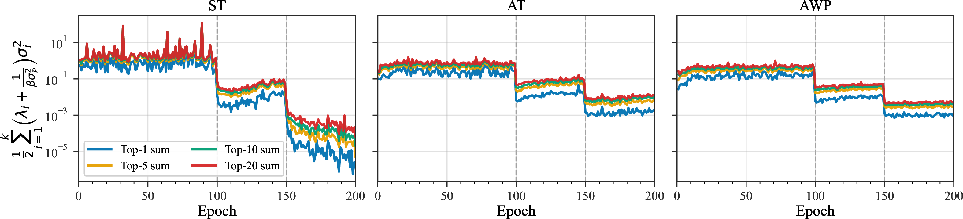
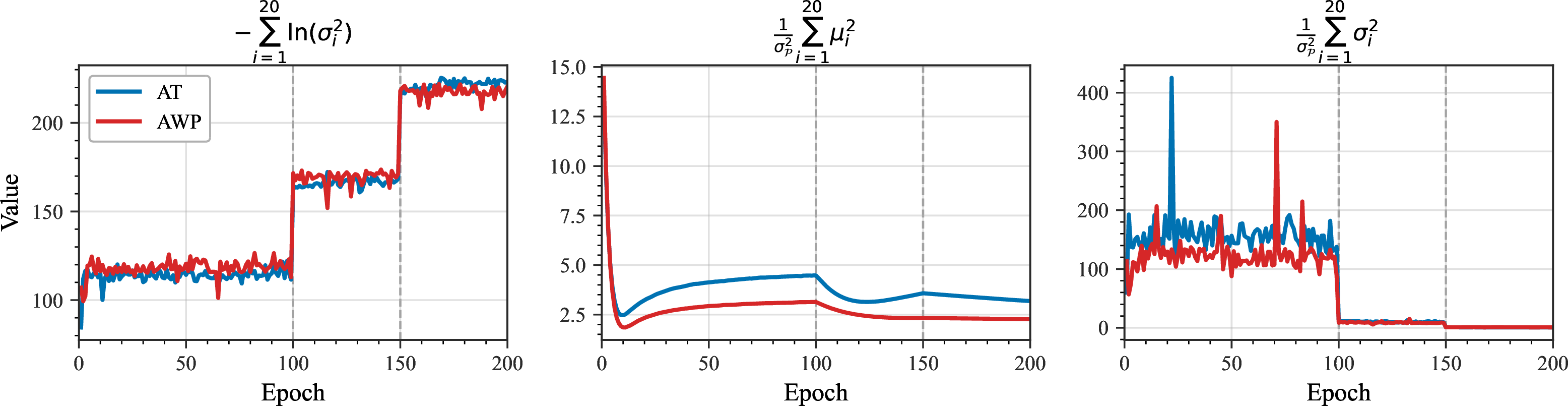
12.2 Full KL and Omitted-Term Diagnostics↩︎

The strict bound in Theorem 3 contains KL terms beyond the log-determinant proxy emphasized in the main diagnostic grid. To ensure the rigor of our analysis and avoid overlooking bound components that may have a critical impact on adversarially robust generalization, we run additional experiments to analyze all KL-related terms and their relative importance. The results are reported in Figure 4 and Figure 5.

In particular, the covariance-trace part of the KL shifts the curvature-weighted variance: \[\text{from}\quad \frac{1}{2}\sum_i\lambda_{t,i}\sigma_{t,i}^2 \quad\text{to}\quad \frac{1}{2}\sum_i\left(\lambda_{t,i}+\frac{1}{\beta\sigma_{\mathcal{P}}^2}\right)\sigma_{t,i}^2.\] For CIFAR-10 with \(|\mathcal{S}|=50{,}000\), we use \(\beta=\sqrt{|\mathcal{S}|}\) and the initialization-matched prior scale \(\sigma_{\mathcal{P}}^2\approx4.93\times10^{-4}\), which gives \(1/(\beta\sigma_{\mathcal{P}}^2)\approx9.07\). Figure 4 visualizes the diagnostic curves with consideration of this extra KL term. The results suggest that the qualitative temporal trends are not affected by including the KL covariance-trace term, which can be absorbed by the more dominant curvature-weighted variance term in our analytical framework.

In Figure 5, we further visualize the diagnostic curves of the remaining KL-related terms (mean-norm component and covariance-trace component) for both AT and AWP. After the learning rate drops, both terms become much smaller than the log-determinant KL component, suggesting negligible influence on robust generalization/overfitting.

12.3 Generalizability Study↩︎

To test the robustness of the diagnostic pattern, we repeat the unified diagnostic grids under variations of (i) dataset/learning algorithm, (ii) perturbation radius \(\epsilon\), (iii) batch size \(B\), and (iv) architecture, objective, dataset, and learning-rate schedule. All plotted quantities and curve definitions match Figures 1 and 2 in the main text: loss/error (top row), leading Hessian eigenvalues \(\{\lambda_i\}\) (second row), projected gradient-noise variances \(\{\gamma_i\}\) (third row), and the resulting bound decomposition terms (variance/entropy/bias; bottom rows). Our goal is not only to document how these curves shift across settings, but also to connect the shifts back to the theory-motivated diagnostics: larger curvature is associated with smaller inferred posterior variances, stronger gradient noise is associated with larger \(\gamma_i\), and robust-overfitting regimes coincide with learning-rate changes that upset this balance and produce posterior-collapse signatures.

Datasets and Learning Algorithms. Figure 6 extends our analysis to CIFAR-100, SVHN, and semi-supervised adversarial training (SSAT) [6]. For CIFAR-100 and SVHN, we use the same epoch budget and learning-rate decay strategy as CIFAR-10: \(200\) epochs with the same piecewise decay points (epochs \(100\) and \(150\)). We keep the optimizer (momentum SGD with \(\kappa=0.9\) and weight decay \(5\times10^{-4}\)) and batch size (\(128\)) fixed. We use an initial learning rate of \(0.1\) for CIFAR-100 and \(0.01\) for SVHN; other attack hyperparameters follow the CIFAR-10 setting unless stated otherwise (for SVHN, we use a smaller PGD step size \(1/255\)).

Relative to CIFAR-10, CIFAR-100 exhibits substantially larger leading curvature and projected noise in the dominant modes (larger \(\lambda_1\) and \(\gamma_1\)), with correspondingly larger magnitudes in the PAC-Bayes proxy terms after learning-rate decays. The post-decay regime shows sharper transients and stronger late-stage degradation in robust test performance, consistent with more pronounced robust overfitting. In contrast, SVHN displays smaller \(\lambda\) and \(\gamma\) trajectories and a smoother post-decay evolution, and its bound components evolve more steadily with weaker evidence of abrupt contraction. SSAT typically lowers risk curves relative to the purely supervised AT baseline, but its geometry does not exhibit the same systematic curvature suppression as AWP; accordingly, its spectra and bound terms fall between standard AT and AWP-like behavior.

These cross-dataset differences are consistent with a margin-distribution view of robust optimization. Harder, fine-grained classification (CIFAR-100) keeps a larger fraction of training points near the adversarial decision boundary, so the inner maximization continues to surface high-sensitivity examples later into training. This sustains sharp Gauss–Newton curvature modes in the robust loss and increases the variability of projected gradients, raising both \(\lambda_i\) and \(\gamma_i\) in the dominant subspace. In our dynamical PAC-Bayes instantiation, larger curvature is associated with stronger posterior contraction and more pronounced posterior-collapse diagnostics, while larger noise inflates \(\sigma_i^2\); after learning-rate decays reduce the step size, this balance can shift toward stronger posterior-contraction signatures.

SVHN is relatively easy for the same architecture: margins are larger, and the adversarial maximization is less likely to produce strongly boundary-adjacent updates, resulting in a smaller dominant spectrum and a more stable curvature–noise balance. Finally, SSAT introduces additional constraints (via unlabeled examples) that can improve generalization, but it does not explicitly penalize weight-space sharpness as AWP does; hence, while risk curves improve, sharp directions need not be systematically suppressed, and the bound decomposition remains closer to AT than to AWP.

Perturbation Radius. Perturbation radius \(\epsilon\) indicates the strength of the inner maximization and thus affects the geometry of the robust objective. Figure 7 reports AT runs with \(\epsilon\in\{2/255,4/255,12/255\}\) (the baseline \(\epsilon=8/255\) is shown in the AT column of Figures 1 and 2). As \(\epsilon\) increases, the dominant curvature modes become systematically sharper (both \(\lambda_1\) and the top-\(k\) averages increase), and the robust test loss/error worsens. Projected noise variances also increase, indicating that stronger attacks not only steepen the robust objective but also change the variability of mini-batch gradients in the sharp subspace. These spectral shifts propagate into the bound decomposition: larger \(\epsilon\) yields larger curvature-weighted variance proxies and typically larger entropy penalties, consistent with a tighter inferred posterior and weaker robust generalization.

This trend is expected because a larger \(\epsilon\) expands the feasible set of adversarial perturbations and strengthens the inner maximization. Training updates may then repeatedly accommodate harder, boundary-adjacent perturbations, which sustain sharp curvature modes in the robust loss for longer and amplify their magnitudes. In the dynamical PAC-Bayes instantiation, posterior contraction associated with curvature (through \(\lambda_i\)) competes with noise-driven inflation (through \(\gamma_i\)). Our ablations suggest that, as \(\epsilon\) increases, the geometric tightening induced by sharper curvature is a dominant contributor to late-stage robust generalization degradation, even though the noise level also changes; this supports interpreting robust overfitting through posterior contraction when the curvature–noise balance becomes unfavorable after learning-rate drops.

Batch Size. In these experiments, batch size primarily changes the estimated gradient-noise level: larger batches reduce the stochasticity of SGD updates and shrink the projected noise variances. Figure 8 compares \(B\in\{64,128,256\}\) (note that \(B=128\) matches our default AT setting in Figures 1 and 2). Across batch sizes, the curvature trajectories (\(\lambda\)) remain comparatively similar, while the projected noise variances (\(\gamma\)) shift by orders of magnitude: smaller batches produce larger \(\gamma_i\), and larger batches suppress them. These shifts are reflected in the bound decomposition. Larger batches correspond to smaller inferred posterior variances \(\sigma_i^2\) and therefore larger entropy proxies \(-\sum \ln\sigma_i^2\), and they are accompanied by stronger late-stage degradation in robust test performance.

Under our stationary (and transient-window) approximations, the per-mode posterior variance scales with the projected noise level, \(\sigma_i^2 \propto \gamma_i\) (modulated by learning rate, momentum, and curvature). Increasing \(B\) reduces \(\gamma_i\), which contracts \(\sigma_i^2\) and inflates the log-determinant (entropy) contribution to the KL term in the PAC-Bayes bound. This yields a dynamical view of a posterior-contraction diagnostic pattern: with insufficient noise injection (large \(B\)), the effective posterior volume shrinks rapidly, and the bound becomes dominated by KL/entropy penalties in sharp directions, especially after learning-rate decays. Smaller batches inject more noise, maintain larger posterior variances, and can delay entry into this collapse-dominated regime, thereby mitigating robust overfitting in the same curvature landscape.

Other Variations. Finally, we report extended diagnostics across architecture, learning rate schedules, objectives, and datasets, without altering the paper’s central experimental design. Figures 9 and 10 use the same six-row grid format as the generalizability figures above, so each setting is shown with loss/error, curvature, noise, and bound-component diagnostics in one place. We use WRN-34-10 [50] to test a higher-capacity architecture than the default PreActResNet-18, TRADES [4] to test an objective-level change to adversarial training, Imagenette-160 [51] to test a higher-resolution natural-image setting beyond CIFAR-scale inputs, and schedule variants to isolate learning-rate transitions. Unless otherwise stated, CIFAR-10 settings use \(\ell_\infty\) perturbations at \(\epsilon=8/255\); Imagenette-160 uses \(\ell_\infty\) perturbations at \(\epsilon=4/255\). The sharp two-drop schedule uses \(0.1\) for epochs \(0\)–\(99\), \(0.001\) for epochs \(100\)–\(149\), and \(10^{-5}\) afterward. The one-drop schedule uses \(0.1\) before epoch \(100\) and \(0.01\) afterward.

These results show that the diagnostic pattern is not tied to the default PreActResNet-18/CIFAR-10/AT configuration. For WRN-34-10, the robust test loss increases after the learning-rate drop while the leading curvature and log-determinant diagnostics grow, consistent with the posterior-contraction pattern observed in the default AT run. The schedule variants isolate the role of learning-rate transitions: the sharp two-drop schedule produces abrupt changes in the variance and entropy diagnostics at the scheduled drops, whereas the one-drop schedule shows a milder post-drop increase in curvature and projected noise. The TRADES and Imagenette-160 runs preserve the same qualitative organization of the diagnostics: increases in leading curvature and projected noise are accompanied by larger curvature-weighted variance and log-determinant terms. These results support using the proposed diagnostic as a stress test across architecture, objective, dataset, and schedule choices, without changing the main claims or treating the top-\(k\) proxies as calibrated full-dimensional bounds.

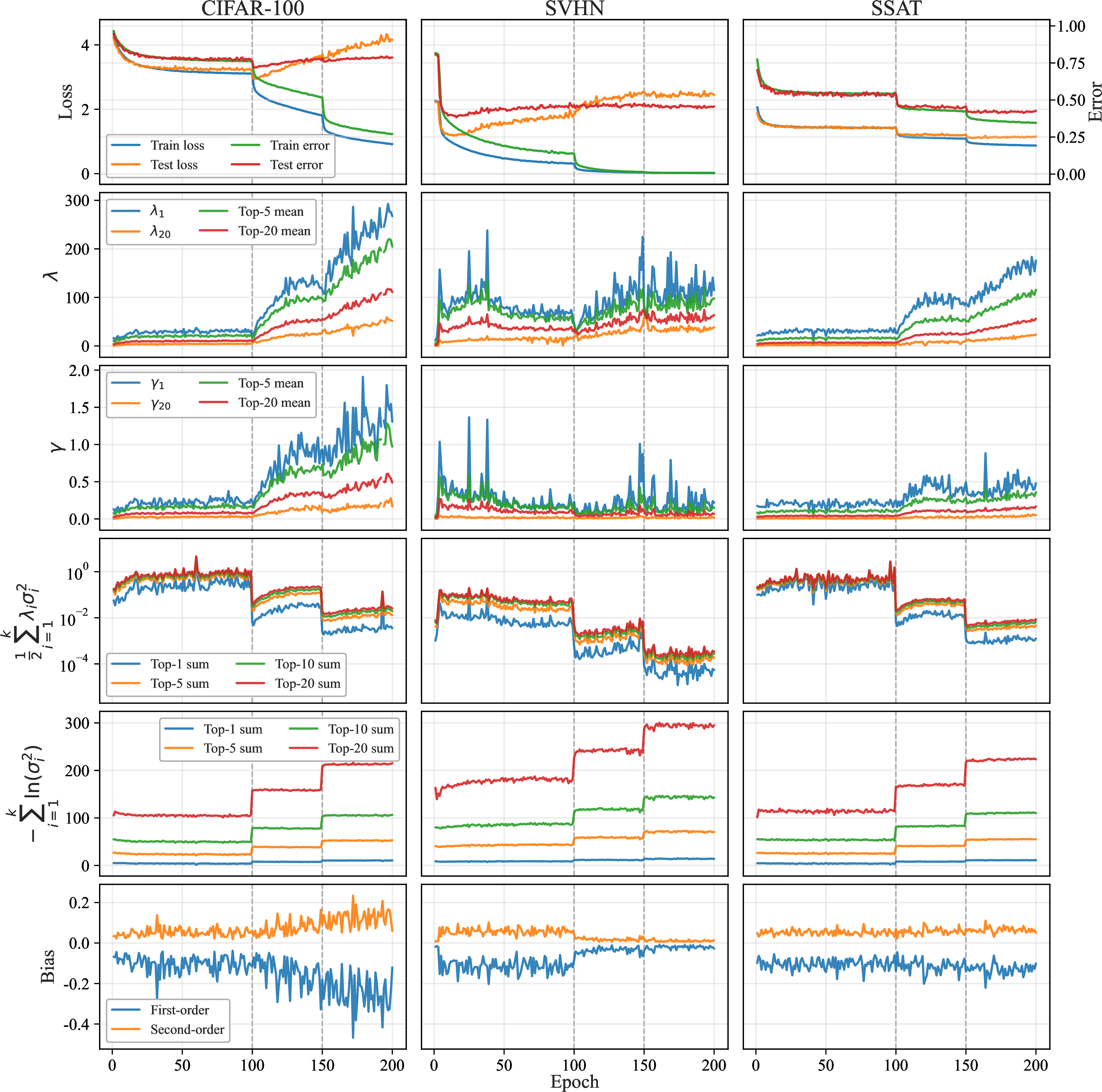
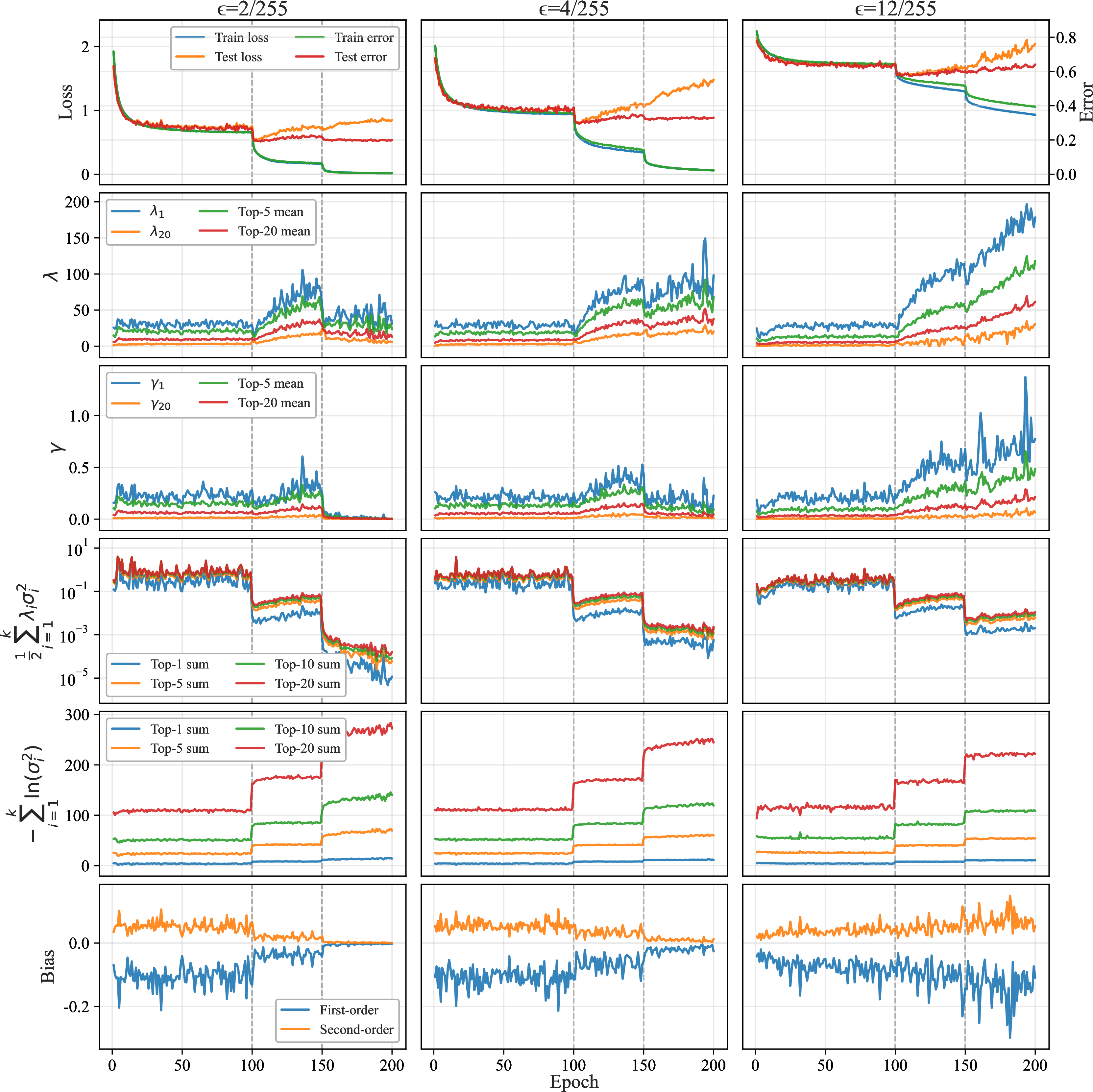
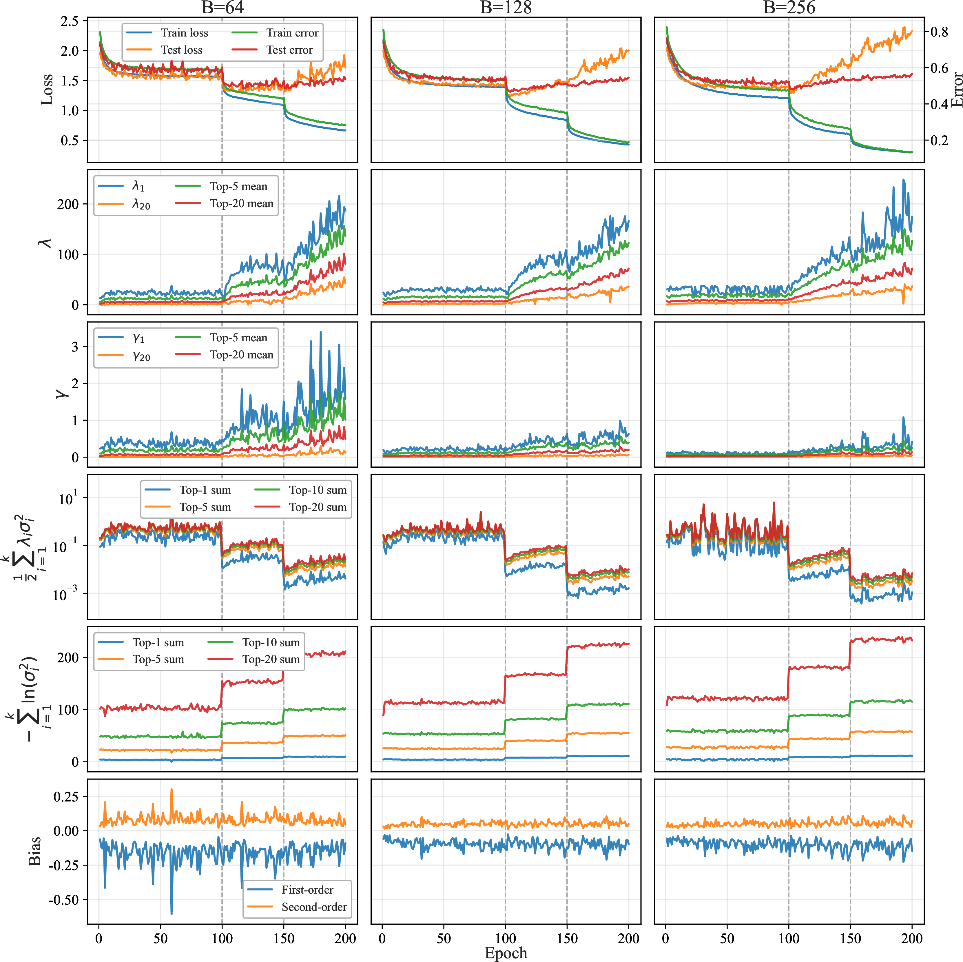
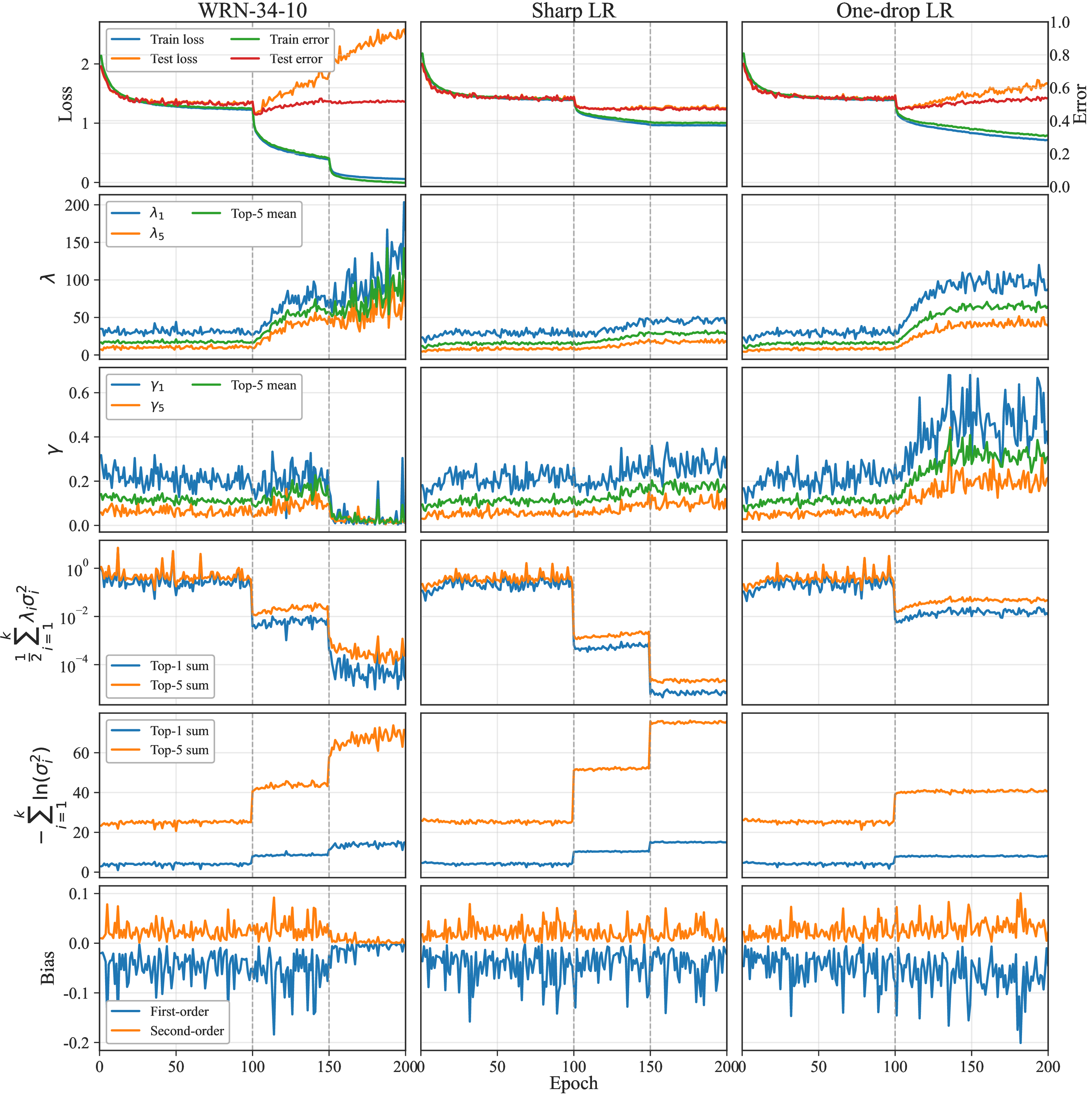
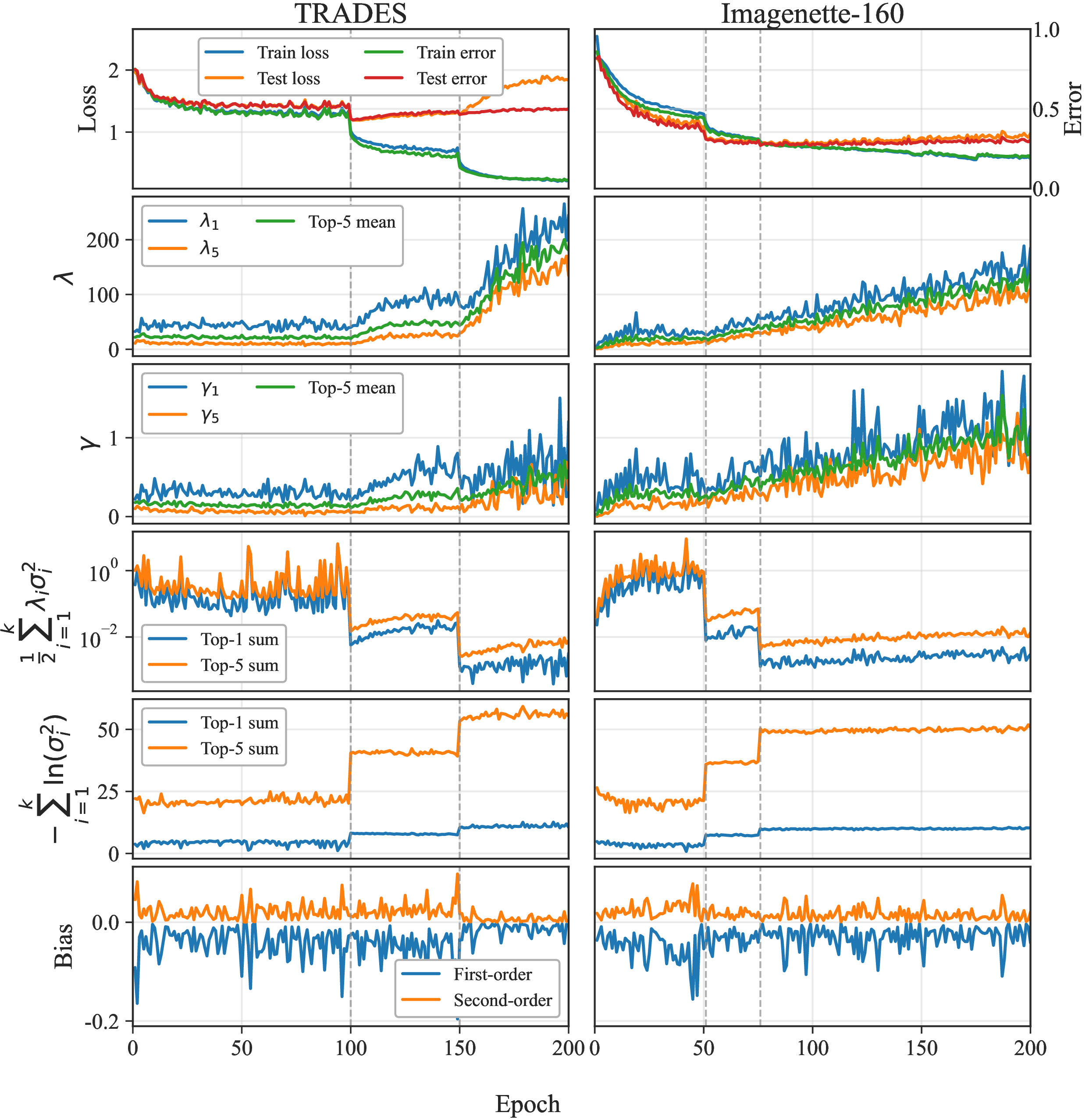
References↩︎

---

1. For cross-entropy loss, one can derive similar concentration results by applying PAC-Bayes-Chernoff bounds [37] for unbounded losses under light-tail or moment conditions.↩︎

2. We ignore \(\hat{\mathcal{L}}_{\epsilon}(\tilde{\boldsymbol{w}}_t)\), \(R_t\) and \(C_{\mathrm{PB}}\) in our later diagnostic analysis, since they are either independent of \(\mathcal{Q}\) or have negligible impact on robust generalization gap compared to remaining terms.↩︎