Theorem 4. There are queries that are expressible in positive recursive SQL, and in linear Datalog, and yet are not expressible in Core GQL nor Core PGQ.
GQL and SQL/PGQ: Theoretical Models and Expressive Power
September 02, 2024
Abstract
SQL/PGQ and GQL are very recent international standards for querying property graphs: SQL/PGQ specifies how to query relational representations of property graphs in SQL, while GQL is a standalone language for graph databases. The rapid industrial development of these standards left the academic community trailing in its wake. While digests of the languages have appeared, we do not yet have concise foundational models like relational algebra and calculus for relational databases that enable the formal study of languages, including their expressiveness and limitations. At the same time, work on the next versions of the standards has already begun, to address the perceived limitations of their first versions.
Motivated by this, we initiate a formal study of SQL/PGQ and GQL, concentrating on their concise formal model and expressiveness. For the former, we define simple core languages – Core PGQ and Core GQL – that capture the essence of the new standards, are amenable to theoretical analysis, and clarify the difference between PGQ’s bottom up evaluation versus GQL’s linear, or pipelined approach. Equipped with these models, we both confirm the necessity to extend the language to fill in the expressiveness gaps and identify the source of these deficiencies. We complement our theoretical analysis with an experimental study, demonstrating that existing workarounds in full GQL and PGQ are impractical, further underscoring the necessity to correct deficiencies in language design.
PVLDB Reference Format:
Amelie Gheerbrant, Leonid Libkin, Liat Peterfreund, and Alexandra Rogova. . PVLDB, 18(6): 1798 - 1810, 2025.
doi:10.14778/3725688.3725707
1 Introduction↩︎
In the past two years, ISO published two new international standards. SQL/PGQ, released in 2023, as Part 16 of the SQL standard, provides a mechanism for representing and querying property graphs in relational databases using SQL. GQL, released in 2024, is a standalone graph query language that does not rely on a relational representation of graphs. SQL/PGQ and GQL are developed in the same ISO committee that has been maintaining and enhancing the SQL standard for decades. These developments reflect the interest of relational vendors in implementing graph extensions and the emergence of a new native graph database industry.
There is however a notable difference between this standardization effort and that of SQL as it happened in the 1980s. Before SQL was designed, strong theoretical and practical foundations of relational databases had been developed. Equivalence of relational algebra and calculus (first-order logic) had been known; these provided very clean abstractions of relational languages that served as the basis of relational database theory. This has had a profound impact on both the theory and the practice of database systems. For example, a question of central importance in the early days of relational databases was expressiveness of query languages, with Fagin, Aho, Ullman, Gaifman, and Vardi independently showing that relational calculus cannot define the transitive closure of a relation [1]–[3]. This led to subsequent development of Datalog and culminated in the inclusion of linear recursive queries by the SQL standard in 1999 [4].
When it comes to graphs, the adoption of languages by industry runs well ahead of the development of their foundational underpinnings. For many years, work on graph queries concentrated on regular path queries (RPQs) [5] and their multiple extensions (e.g., [6]–[9], crpq?). These however assume a much simplified model in which neither nodes nor edges have properties, unlike property graphs preferred in industry. A step in that direction is the model of data graphs in which nodes but not edges carry data [10]. To this day, these models are the basis of work on query language expressiveness [11], [12]. But we will see soon that from the point of view of GQL and SQL/PGQ, a full property graph model makes a huge difference. Existing theoretical languages such as GXPath [10], regular queries [13], STRUQL [14], while having a direct influence on the design of GQL [15], are not a good reflection of it.
At the same time, extensive discussions in the standards committees are already under way to identify new features of SQL/PGQ and GQL, based on their perceived, rather than proved, shortcomings [16], [17]. These considerations motivate our main contributions:
We provide concise formal models of SQL/PGQ and GQL;
We confirm the intuition that certain queries of interest to customers of graph databases cannot be expressed by SQL/PGQ and GQL patterns;
We compare GQL with recursive SQL and show that the latter is more powerful; and
We show experimentally that methods currently allowed in SQL/PGQ and GQL to overcome these limitations are impractical, even for small-sized graphs.
We now elaborate more on these goals.
1.0.0.1 Formal models of GQL and SQL/PGQ
The workhorse of graph query languages is pattern matching. In Cypher, PGQ, GQL and others, pattern matching turns a graph into a table; the remaining operations of the language manipulate that table. In fact in GQL and SQL/PGQ pattern matching is identical; it is only how its results are processed that is different. In SQL/PGQ, a graph is a view defined on a relational database. The result of pattern matching is simply a table in the clause of a SQL query that may use other relations in the database. GQL, on the other hand, is oblivious to how a graph is stored, and the table resulting from pattern matching is manipulated by a sequence of operators that modify it, in an imperative style that is referred to as “linear composition”.
To produce a formal model of these languages, we use the relationship between SQL and relational calculus/algebra as the guiding principle. SQL has a multitude of features: bag semantics, nulls, arithmetic operations, aggregate functions, outerjoins, complex datatypes such as arrays. Some of these break the theoretical model of First Normal Form (1NF) relations which are sets of tuples of atomic values. Relational algebra and calculus get rid of the extra baggage that SQL is forced to add to be usable in practice, and yet provide a simple core over sets of tuples of atomic values.
Although some mathematical abstractions of GQL and SQL/PGQ exist [18], [19], they are not yet at the same level as RA or relational calculus, in terms of their simplicity and utility in formally proving results. For example, their formalizations of pattern matching come with a complex typing system and the use of conditional and group variables that create nulls and set-valued attributes. To achieve our goal of creating a simple and usable abstraction, we need to: simplify the model of pattern matching, to avoid outputting non-1NF relations, and to formalize the linear composition of Cypher and GQL. This allows us to define two languages – Core PGQ and Core GQL – as RA or linear composition of relational operators on top of pattern matching outputs.
1.0.0.2 Limitations of pattern matching
Many pattern matching tasks require iterating patterns, notably when we do not know a priori the length of a path we are searching for (a basic example is reachability in graphs). The way pattern matching is designed in Cypher, GQL, and SQL/PGQ, makes it easy to compare two consecutive iterations of a pattern based on property values of their nodes, but at the same time it is very hard to compare property values in edges.
To illustrate this, assume we have a chain of transfers between accounts: accounts are nodes, with property values such as “balance”, and transfers are edges, with property values such as “amount” and “timestamp”, between accounts. It is very easy to write a query looking for a chain of transfers such that the balance increases in accounts along the chain. It appears to be very hard or impossible to write a query looking for a chain of transfers such that the timestamp increases along the path.
Demand for these queries occurs often in practice, which forced several companies participating in GQL design in ISO to start thinking of language extensions that will permit such queries [16], [17]. However, before making non-trivial language enhancements, it would be good to actually know that newly added features cannot be achieved with what is already in the language.
We show that this is indeed the case. Equipped with our formalization of the pattern language, we prove that it cannot express a large class of queries that analyze how property values of edges change along matched paths; of these the increasing value in edges query is the simplest. This follows in fact from a more general property that is akin to a pumping lemma for paths that can be selected by GQL and PGQ patterns.
1.0.0.3 GQL vs Recursive SQL vs Datalog
When the ubiquitous CRPQs was introduced in crpq?, it was shown that a Datalog-like language based on CRPQs has the power of transitive closure logic [20] and captures the complexity class \(\mathrm{\small NLogSpace}\)of problems solved by nondeterministic Turing machines whose work tape used logarithmic number of bits in terms of the size of the input (this class is contained in polynomial time). Since then, \(\mathrm{\small NLogSpace}\)is the yardstick complexity class we compare graph languages to, and Datalog – that subsumes the transitive closure logic – is a typical language used to understand the power of graph querying.
Datalog is also the basis of SQL’s recursive common table expressions (CTE) introduced by the clause. In fact, in SQL only linear Datalog rules are allowed: in them, the recursively defined predicate can be used at most once.
Motivated by this, we compare the power of GQL with recursive SQL and linear Datalog. We show that there are queries that are expressible in the latter, have very low data complexity, and yet are not expressible in GQL. We explain how this points out deficiencies of GQL design that will hopefully be addressed in the future.
1.0.0.4 Experimental evaluation: can graph DBMSs overcome these limitations?
Real-life systems go beyond basic calculi; SQL with recursion and aggregates is in fact Turing-complete and thus can express all computable queries. Similarly, GQL, PGQ, Cypher and others have many tools at their disposal to let users write very powerful queries. In fact queries such as increasing value in edges are expressible in real-life Cypher and PGQ, though in a very convoluted way. Since the complement of the query is easily expressible, one can look for all the paths and then subtract the complement. Intuitively, such a way should not work in practice as the number of paths in a graph grows exponentially.
This is precisely what we confirm using three different implementation of graph database queries: Neo4j and Memgraph for Cypher, and DuckDB for SQL/PGQ. Native graph systems can handle just a few dozen nodes before 100% timeout rate is observed; DuckDB does marginally better as it computes fewer paths to start with. It is important to note that this is not a critique of the systems tested, as the indirect method of computing the query inherently requires an exponential number of paths. Instead, this confirms that no workaround can bypass the inherent expressibility limitations.
Since inexpressibility results are commonly used to identify deficiencies in language design, and serve as a motivation to increase language expressiveness, we shall at the end of the paper discuss what these results tell us in terms of new features of GQL and SQL/PGQ that will be required.
Related work↩︎
While industry is dominated by property graphs (Neo4j cypher?, Oracle [21], Amazon [22], TigerGraph [23], etc), much of academic literature still works with the model of labeled graphs and query languages based on RPQs, with some exceptions [10], [24], [25]. However, the rare models focused on property graphs appeared before the new standards became available, and their analyses of expressiveness and language features do not apply to GQL and SQL/PGQ. The first commercial language for property graphs was Cypher, and it was fully formalized in cypher?. As GQL and SQL/PGQ were being developed, a few academic papers appeared. For example, [26] gave an overview of their pattern matching facilities, which was then further analyzed in [19], and [27] provided a description of an early implementation of SQL/PGQ.
In [18], a digest of GQL suitable for the research community was presented. While a huge improvement compared to the actual standard from the point of view of clarity, the presentation of [18] replaced 500 pages of the text of the Standard (notoriously hard to read) by a one-page long definition of the syntax, followed by a four-pages long definition of the semantics. It achieved a two orders of magnitude reduction in the size of the definition of the language, but 5 pages is still way too long for “Definition 1”. The language of [19] is closer to our goal, but it is not well-suited to the level reasoning we require here as it still contains still too much of the GQL and PGQ baggage, for example non-1NF relations, and a complex type system for singleton, conditional, and group variables that we avoid here entirely and replace by the very familiar definition of free variables.
Another element missing from the literature is a proper investigation of linear composition. Initially introduced in Cypher, it was then adopted in a purely relational language PRQL [28] (positioned as “pipelined” alternative to SQL), embraced by GQL, and influenced the designed of the piped SQL syntax [29]; however formal analyses of this way of building complex queries are lacking.
2 GQL and SQL/PGQ by examples↩︎
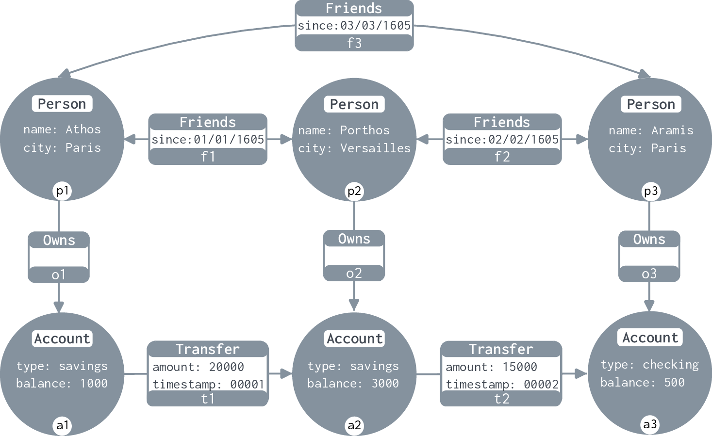
We illustrate GQL and SQL/PGQ capabilities using the graph from Figure 1 and the following money-laundering query: Find a pair of friends in the same city who transfer money to each other via a common friend who lives elsewhere. Notice that we assume that friendship is a symmetric relation.
In GQL, it will be expressed as query:
MATCH (x)-[:Friends]->(y)-[:Friends]->(z) -[:Friends]->(x), (x)-[:Owns]->(acc_x), (y)-[:Owns]->(acc_y), (z)-[:Owns]->(acc_z), (acc_x)-[t1:Transfer]->(acc_z) -[t2:Transfer]->(acc_y) FILTER (y.city = x.city) AND (x.city<>z.city) AND (t2.amount < t1.amount) RETURN x.name AS name1, y.name AS name2
In SQL/PGQ, a graph is a view of a tabular schema. The graph from Figure 1 can be represented by the following set of tables:
Person(p_id,name,city)for people,Acc(a_id,type)for accounts,Friend(p_id1,p_id2,since)for friendships,Owns(a_id,p_id)for ownership andTransfer(t_id,a_from,a_to,amount)for transfers.
The property graph view is then defined by a \(\text{\normalfont\small\renewcommand{\ttdefault}{pcr}\ttfamily\bfseries\color{darkblue} CREATE}\) statement, part of which is shown below:
CREATE PROPERTY GRAPH Interpol1625 ( VERTEX TABLES Acc KEY (a_id) LABEL Account PROPERTIES (type) .… EDGE TABLES Transfer KEY (t_id) SOURCE KEY (a_from) REFERENCES Acc DESTINATION KEY (a_to) REFERENCES Acc LABEL Transfer PROPERTIES (amount) .… )
This view defines nodes (vertices) and edges of the graph, specifies endpoints of edges, and defines their labels and properties. We can then query it, using pattern matching to create a subquery:
SELECT T.name_x AS name1, T.name_y AS name2 FROM Interpol1625 GRAPH_TABLE ( MATCH (x)-[:Friends]->(y)-[:Friends]->(z) -[:Friends]->(x), (x)-[:Owns]->(acc_x), (y)-[:Owns]->(acc_y), (z)-[:Owns]->(acc_z), (acc_x)-[t1:Transfer]->(acc_z) -[t2:Transfer]->(acc_y) COLUMNS x.city AS city_x, y.city AS city_y, z.city AS city_z, x.name AS name_x, y.name AS name_y, t1.amount AS amnt1, t2.amount AS amnt2 ) AS T WHERE T.city_x=T.city_y AND T.city_x <> T.city_z AND T.amount1 > T.amount2
Note that in GQL, a sequence of operators can continue after the \(\text{\normalfont\small\renewcommand{\ttdefault}{pcr}\ttfamily\bfseries\color{darkblue} RETURN}\) clause. For example, if we want to find large transfers between the two potential offenders we could simply continue the first GQL query with extra clauses:
MATCH (u WHERE u.name=name1) -[t:Transfer]-> (v WHERE v.name=v2) FILTER t.amount > 100000 RETURN t.amount AS big_amount
This is what is referred to as linear composition: we can simply add clauses to the already existing query which apply new operations to the result of already processed clauses.
In SQL/PGQ, such an operation is also possible, though perhaps a bit more cumbersome as we would need to put the above PGQ query as a subquery in and create another subquery for the second match, then join them on name1 and
name2.
3 Pattern Matching: Turning Property Graphs into Relations↩︎
We define property graphs and pattern matching, the key component of GQL and SQL/PGQ, that extracts relations from graphs.
3.1 Property Graphs↩︎
We use the standard definition (cf. [19]), and only consider directed edges. Assume pairwise disjoint countable sets \(\mathcal{L}\) of labels, \(\mathcal{K}\) of keys, \(\mathsf{Const}\) of constants, \(\mathsf{N}\) of node ids, and \(\mathsf{E}\) of edge ids.
Definition 1 (Property Graph). A property graph is a tuple \(G= \langle N, E, \mathsf{lab}, \mathsf{src}, \mathsf{tgt}, \mathsf{prop}\rangle\) where
\(N \subset \mathsf{N}\) is a finite set of node ids used in \(G\);
\(E \subset \mathsf{E}\) is a finite set of directed edge ids used in \(G\);
\(\mathsf{lab}: N \cup E \to 2^{\mathcal{L}}\) is a labeling function that associates with every node or edge id a (possibly empty) finite set of labels from \(\mathcal{L}\);
\(\mathsf{src}, \mathsf{tgt}: E \to N\) define source and target of an edge;
\(\mathsf{prop}: (N \cup E) \times \mathcal{K}\to \textsf{Const}\) is a partial function that associates a property value with a node/edge id and a key.
A path in \(G\) is an alternating sequence \(u_0 e_1 u_1 e_2 \cdots e_{n} u_n\), for \(n \geq 0\), of nodes and edges that starts and ends with a node and so that each edge \(e_i\) connects the nodes \(u_{i-1}\) and \(u_i\) for \(i \leq n\). More precisely, for each \(i \leq n\), either \(\mathsf{src}(e_i)=u_{i-1}\) and \(\mathsf{tgt}(e_i)=u_i\) (a forward edge), or \(\mathsf{src}(e_i)=u_{i}\) and \(\mathsf{tgt}(e_i)=u_{i-1}\) (a backward edge). Note that \(n=0\) is possible, in which case the path consists of a single node \(u_0\). We shall explicitly spell out paths as \(\textsf{path}(u_0,e_1,u_1,\cdots, e_n,u_n)\).
Two paths \(p = \textsf{path}(u_0,e_0,\ldots,u_k)\) and \(p' = \textsf{path}(u'_0,e'_0,\ldots,u'_j)\) concatenate, written as \(p \odot p'\), if \(u_k = u'_0\), in which case their concatenation \(p \cdot p'\) is defined as \(\textsf{path}(u_0,e_0,\ldots,u_k,e'_0,\ldots,u'_j)\). Note that a single-node path is a unit of concatenation: \(p \cdot\textsf{path}(u)\) is defined iff \(u=u_k\) and is equal to \(p\).
3.2 Pattern Matching↩︎
Pattern matching is the key component of graph query languages. As already mentioned, an early abstraction of GQL and PGQ patterns was given in [19], but it retained too much of the baggage of the actual language (non-1NF outputs, nulls, a complex type system) for language analysis. Thus, here we refine the definitions from [19] to capture the core concepts of pattern matching, similarly to relational algebra for relational databases. To this end, we fix an infinite set \(\mathsf{Vars}\) of variables and define Core GQL and Core PGQ pattern matching as follows:
\(\psi\;\;:=\;\; (x) \;\mid \; \overset{x}{\rightarrow} \;\mid \; \overset{x}{\leftarrow} \;\mid \; \psi_1\, \psi_2 \;\mid\; \psi^{n..m} \;\mid\; \psi\langle\theta \rangle \;\mid \; \psi_1 + \psi_2\)
where
\(x \in \mathsf{Vars}\) and \(0 \leq n \leq m \leq \infty\);
variables \(x\) in node and edge patterns \((x)\), \(\overset{x}{\rightarrow}\), and \(\overset{x}{\leftarrow}\) are optional,
\(\psi\langle\theta \rangle\) is a conditional pattern, and conditions are given by \(\theta, \theta' \;:=\;x.k=x'.k' \mid x.k<x'.k' \mid \ell(x) \mid \theta \vee \theta' \mid \theta \wedge \theta' \mid \neg \theta\) where \(x,x'\in\mathsf{Vars}\) and \(k,k'\in\mathcal{K}\);
\(\psi_1+\psi_2\) is only defined when their sets of free variables \(\mathsf{FV}\left(\psi_1\right)\) and \(\mathsf{FV}\left(\psi_2\right)\) are equal.
The sets of free variables are defined as follows:
\(\mathsf{FV}\Big((x)\Big) = \mathsf{FV}\left(\overset{x}{\rightarrow}\right) = \mathsf{FV}\left( \overset{x}{\leftarrow}\right) \;:=\;\{x\}\);
\(\mathsf{FV}\left(\psi_1 + \psi_2\right) \;:=\; \mathsf{FV}\left(\psi_1\right)\)
\(\mathsf{FV}\left( \psi_1\, \psi_2 \right) \;:=\;\mathsf{FV}\left(\psi_1\right)\cup\mathsf{FV}\left( \psi_2 \right)\)
\(\mathsf{FV}\left( \psi^{n..m} \right) \;:=\;\emptyset\)
\(\mathsf{FV}\left(\psi\langle\theta \rangle\right) \;:=\;\mathsf{FV}\left(\psi\right)\)
A pattern produces an output that consists of graph elements and their properties. Such an output \(\Omega\) is a (possibly empty) tuple whose elements are either variables \(x\) or properties \(x.k\). A pattern with output, or, pattern, for simplicity, is an expression \(\psi_\Omega\) such that every variable present in \(\Omega\) is in \(\mathsf{FV}\left(\psi\right)\).
3.2.0.1 Correspondence with Cypher and GQL
For the reader familiar with Cypher and/or GQL, we explain how our fomalization compares with these languages’ patterns.
\((x)\) is a node pattern that binds the variable \(x\) to a node;
\(\overset{x}{\rightarrow}\) and \(\overset{x}{\leftarrow}\) are forward edge and backward edge patterns, that also bind \(x\) to the matched edge;
\(\psi_1\, \psi_2\) is the concatenation of patterns,
\(\psi^{n..m}\) is the repetition of \(\psi\) between \(n\) and \(m\) times (with a possibility of \(m=\infty\))
\(\psi\langle\theta \rangle\) corresponds to \(\text{\normalfont\small\renewcommand{\ttdefault}{pcr}\ttfamily\bfseries\color{darkblue} WHERE}\) in patterns, conditions involve (in)equalities between property values, checking for labels, and their Boolean combinations;
\(\psi_1 + \psi_2\) is the union of patterns;
\(\psi_\Omega\) corresponds to the output forming clauses of Cypher and GQL and of SQL/PGQ, with \(\Omega\) listing the attributes of returned relations.
3.2.0.2 Semantics
To define the semantics, we use set \(\mathsf{Values}\) which is the union of \(\mathsf{Const}\cup \mathsf{N}\cup \mathsf{E}\). That is, its elements are node and edge ids, or values of properties, i.e., precisely the elements that can appear as outputs of patterns.
The semantics of a path pattern \(\psi\), with respect to a graph \(G\), is a set of pairs \((p,\mu)\) where \(p\) is a path and \(\mu\) is a mapping \(\mathsf{FV}\left(\psi\right)\rightarrow \mathsf{Values}\). Recall that we write \(\mu_\emptyset\) for the unique empty mapping with \(\mathsf{dom}(\mu)=\emptyset\).
For the semantics of path patterns with output \(\psi_\Omega\) we define \(\mu_\Omega:\Omega\to \mathsf{Values}\) as the projection of \(\mu\) on \(\Omega\): \[\mu_\Omega(\omega) := \begin{cases} \mu(x) & \text{if } \omega= x\in \mathsf{Vars}\\ \mathsf{prop}(\mu(x),k) & \text{if } \omega= x.k\,. \end{cases}\] Full definitions are presented in Figure 2. For node and edge patterns with no variables, the mapping part of the semantics changes to \(\mu_\emptyset\). The satisfaction of a condition \(\theta\) by a mapping \(\mu\), written \(\mu\models\theta\), is defined as follows: \(\mu\models x.k = x'.k'\) if both \(\mathsf{prop}(\mu(x),k)\) and \(\mathsf{prop}(\mu(x'),k')\) are both defined and are equal (and likewise for \(<\)), and \(\mu\models\ell(x)\) if \(\ell\in\mathsf{lab}(\mu(x))\). It is then extended to Boolean connectives \(\wedge, \vee, \neg\) in the standard way.
None
Figure 2: Semantics of patterns and patterns with output.
3.2.0.3 Pattern languages vs GQL and PGQ patterns
Compared to GQL and PGQ patterns as described in [18], [19], [26], we make some simplifications. First and foremost, they are to ensure that outputs of pattern matching are 1NF relations. Similarly to formal models of SQL by means of relational algebra and calculus over sets of tuples, we do not include bags, nulls, and relations whose entries are not atomic values. The differences manifest themselves in four ways.
First, we use set semantics rather than bag semantics. GQL and PGQ pattern can return tables with duplicate patterns; we follow their semantics up to multiplicity.
Second, in disjunctions \(\psi_1 + \psi_2\) we require that free variables of \(\psi_1\) and \(\psi_2\) be the same. In GQL this is not the case, but then for a variable \(x \in \mathsf{FV}\left(\psi_1\right)-\mathsf{FV}\left(\psi_2\right)\), a match for \(\psi_2\) would generate a null in the \(x\) attribute. Following the 1NF philosophy, we omit features that can generate nulls.
Third, repeated patterns \(\psi^{n..m}\) have no free variables. In GQL and PGQ, free variables of \(\psi\) become group variables in \(\psi^{n..m}\), leading to both a complex type system [19] and crucially non-flat outputs. Specifically such variables are evaluated to lists. For example, in the pattern \(()\xrightarrow{x}^{0..\infty}()\), the variable \(x\) would be mapped to the list of edge ids traversed by the path. These lists would be typically represented as values of an type in implementations (cf. [27]) thus again violating 1NF.
Fourth, we do not impose any conditions on paths that can be matched. In GQL and PGQ they can be simple paths (no repeated nodes), or trails (no repeated edges), or shortest paths. In GQL, PGQ, and Cypher, paths themselves may be returned, and such restrictions therefore are necessary to ensure finiteness of output. Since we can only return graph nodes or edges, or their properties, we never have the problem of infinite outputs, and thus we chose not to overcomplicate the definition of core languages by deviating from flat tables as outputs.
In what might look like a simplification w.r.t. GQL and PGQ, we do not have explicit joins of patterns, i.e., \(\psi_1, \psi_2\) with the semantics \(\left\llbracket\psi_1,\psi_2\right\rrbracket_{G} = \left\{\big((p_1,p_2),\mu_1 \bowtie\mu_2\big) \mid (p_i,\mu_i)\in \left\llbracket\psi_i\right\rrbracket_G, \; i=1,2\right\}\). This is because such joins are definable with RA operations. This simplification is in the same spirit as not including the natural join in the definition of RA, since it can already be expressed with product, selection, and projection.
4 SQL/PGQ: Theoretical Abstractions↩︎
Having defined patterns shared by SQL/PGQ and GQL, we can proceed to provide a theoretical abstraction of SQL/PGQ. Recall that in PGQ, the statement is embedded in . In fact results of matches over a graph are simply treated as relations, or subqueries, over which the usual SQL can be asked. Taking again the view that our goal is to provide the core abstraction of the language, on top of which others can be built, we look at the essential core of relational languages, namely relational algebra. With this in mind, we define (for now informally):
To make this definition formal, we define some very standard concepts. We assume an infinite countable set \(\mathcal{S}\) of relation symbols, such that each \(S\in \mathcal{S}\) is associated with a sequence \(\mathsf{attr}(S):=A_1, \ldots, A_n\) of attributes for some \(n>0\); here attributes \(A_i\) come from a countably infinite set \(\mathcal{A}\) of attributes. By \(\mathsf{arity}(S)\) we mean \(n\), and to be explicit about names of attributes write \(S(A_1, \ldots, A_n)\).
Fix an infinite domain \(\mathbf{U}\) of values. A relation over \(S(A_1,\ldots, A_n)\) is a set of tuples \(\mu:\{A_1,\ldots, A_n\} \rightarrow \mathbf{U}\). The domain of \(\mu\) is denoted \(\mathsf{dom}(\mu)\), and we often represent tuples as sets of pairs \((A,\mu(A))\) for \(A\in \mathsf{dom}(\mu)\). A relational database \(\mathcal{D}\) is a partial function that maps symbols \(S\in \mathcal{S}\) to relations \(\mathcal{D}(S)\) over \(S\) (if \(\mathcal{D}\) is clear from the context we refer to \(\mathcal{D}(S)\) simply as \(S\), by a slight abuse of notation.) We say that \(\mathcal{D}\) is over its domain \(\mathsf{dom}(\mathcal{D})\).
Let \(\mu\) be a tuple and \(\pmb{A} \subseteq \mathsf{dom}(\mu)\). We use \(\mu\restriction \pmb{A}\) to denote the restriction of \(\mu\) to \(\pmb{A}\), that is, the mapping \(\mu'\) with \(\mathsf{dom}(\mu') = \pmb{A}\) and \(\mu'(A) :=\mu(A)\) for every attribute \(A\in \pmb{A}\). Two tuples \(\mu_1,\mu_2\) are compatible, denoted by \(\mu_1 \sim \mu_2\), if \(\mu_1(A) = \mu_2(A)\) for every \(A\in \mathsf{dom}(\mu_1) \cap \mathsf{dom}(\mu_2)\). For such compatible tuples define \(\mu_1 \bowtie\mu_2\) as the mapping \(\mu\) with \(\mathsf{dom}(\mu):=\mathsf{dom}(\mu_1) \cup \mathsf{dom}(\mu_2)\), and \(\mu(A):=\mu_1(A)\) if \(A\in\mathsf{dom}(\mu_1)\) and \(\mu(A):=\mu_2(A)\) otherwise.
If \(A\in\mathsf{dom}(\mu)\) then the renaming \(\rho_{ A\rightarrow B}(\mu)\) of \(A\) to \(B\) is the mapping \(\mu'\) with \(\mathsf{dom}(\mu')= (\mathsf{dom}(\mu) \setminus\{A \})\cup\{B\}\) where \(\mu'(B):=\mu(A)\) and \(\mu'(A')= \mu(A')\) for every other \(A'\in\mathsf{dom}(\mu')\).
4.0.0.1 Relational Algebra (RA)
We use a standard presentation of RA. Given a schema \(\mathbf{S}\) which is a finite subset of \(\mathcal{S}\), the expressions \(\mathcal{Q}\) of \(\mathsf{RA}(\mathbf{S})\) and selection conditions \(\theta\) are defined as
\[\begin{array}{rcl} \mathcal{Q}, \mathcal{Q}' & \!\!:=\!\! & R \; \mid \;\pi_{\pmb{A}}(\mathcal{Q}) \; \mid \;\sigma_{\theta}(\mathcal{Q}) \; \mid \;\mathcal{Q}\bowtie\mathcal{Q}' \; \mid \;\mathcal{Q}\cup \mathcal{Q}' \; \mid \;\mathcal{Q}- \mathcal{Q}' \\ \theta & \!\!:=\!\! & A = A' \mid \neg \theta \mid \theta \vee \theta \mid \theta \wedge \theta \end{array}\] where \(R\) ranges over relations in \(\mathbf{S}\). The sets of attributes of expressions \(\mathsf{attr}(\mathcal{Q})\) are defined by extending \(\mathsf{attr}(R)\), namely \(\mathsf{attr}(\pi_{\pmb{A}}(\mathcal{Q}))\) is \(\pmb{A}\), while both of \(\mathsf{attr}(\sigma_{\theta}(\mathcal{Q}))\) and \(\mathsf{attr}( \mathcal{Q}\circ\mathcal{Q}')\) are \(\mathsf{attr}(Q)\), for \(\circ\) being union and difference; \(\mathsf{attr}( \mathcal{Q}\bowtie\mathcal{Q}') = \mathsf{attr}( \mathcal{Q}) \cup \mathsf{attr}( \mathcal{Q}')\) and \(\mathsf{attr}(\rho_{ A \rightarrow A'}(\mathcal{Q})) = (\mathsf{attr}(\mathcal{Q}) \setminus \{ A \})\cup \{ A'\}\).
The expressions of RA must satisfy the usual well-definedness rules: \({\pi_{\pmb{A}}(\mathcal{Q})}\) is well-defined if \(\pmb{A}\subseteq \mathsf{attr}(\mathcal{Q})\); set operations are defined if \(\mathsf{attr}(\mathcal{Q})=\mathsf{attr}(\mathcal{Q}')\), and for renaming from \(A\) to \(A'\) we must have \(A\in\mathsf{attr}(\mathcal{Q})\) and \(A'\not\in\mathsf{attr}(\mathcal{Q})\).
The result of evaluation of a query \(\mathcal{Q}\) on a database \(\mathcal{D}\) is a relation \(\left\llbracket\mathcal{Q}\right\rrbracket_{\mathcal{D}}\) over \(\mathsf{attr}(\mathcal{Q})\) defined as: \[\begin{align} \left\llbracket R\right\rrbracket_{\mathcal{D}} :=\;\;\; & {\mathcal{D}}(R)&\\ \left\llbracket\pi_{\pmb{A}}(\mathcal{Q})\right\rrbracket_{\mathcal{D}} :=\;\;\; & \{ \mu\restriction_{\pmb{A}} \;\mid \;\mu\in \mathcal{Q}\}&\\ \left\llbracket\sigma_{\theta}(\mathcal{Q})\right\rrbracket_{\mathcal{D}} :=\;\;\; & \{ \mu\;\mid\;\mu\in \mathcal{Q}\text{ and } \mu\models \theta\}&\\ \left\llbracket\rho_{ A \rightarrow A'}(\mathcal{Q})\right\rrbracket_{\mathcal{D}}:=\;\;\; &\{ \rho_{ A \rightarrow A'}(\mu) \mid \mu\in \mathcal{Q}\}&\\ \left\llbracket\mathcal{Q}\bowtie\mathcal{Q}'\right\rrbracket_{\mathcal{D}} :=\;\;\; & \{\mu \bowtie\mu' \;\mid \;\mu\in\mathcal{Q}, \;\mu'\in \mathcal{Q}' \}&\\ \left\llbracket\mathcal{Q}\circ\mathcal{Q}'\right\rrbracket_{\mathcal{D}} :=\;\;\; & \left\llbracket\mathcal{Q}\right\rrbracket_{\mathcal{D}} \circ\left\llbracket \mathcal{Q}'\right\rrbracket_{\mathcal{D}}& \text{ for }\circ\in \{\cup,\setminus \} \end{align}\]
with \(\mu\models \theta\) having the standard semantics \(\mu \models A=A'\) iff \(A,A'\in\mathsf{dom}(\mu)\) and \(\mu(A) = \mu(A')\), extended to Boolean connectives \(\wedge, \vee, \neg\).
4.0.0.2 Core PGQ
Assume that for each variable \(x\in\mathsf{Vars}\) and each key \(k\in\mathcal{K}\), both \(x\) and \(x.k\) belong to the set of attributes \(\mathcal{A}\). For each pattern \(\psi\) and each output specification \(\Omega\), we have a relation symbol \(R_{\psi,\Omega}\) whose set of attributes are the elements of \(\Omega\). Let \(\mathsf{Pat}\) contain all such relation symbols.
Definition 2 (Core PGQ). Core PGQ is defined as \(\mathsf{RA}(\mathsf{Pat})\), i.e., the set of relational algebra expressions over the schema \(\mathsf{Pat}\).
To define the semantics of Core PGQ queries, assume without loss of generality that \(\mathsf{Values}\subseteq \mathbf{U}\). This ensures that results of pattern matching are relations of the schema \(\mathsf{Pat}\), because for every path pattern with output \(\psi_{\Omega}\) and a property graph \(G\), the table \(\left\llbracket\psi_{\Omega}\right\rrbracket_{G}\) is an instance of relation \(R_{\psi,\Omega}\) from \(\mathsf{Pat}\).
Then the semantics of Core PGQ is simply the extension of the semantics of \(\mathsf{RA}\) defined above where for base relations we have
\(\left\llbracket R_{\psi,\Omega}\right\rrbracket_G\;:=\;\left\llbracket\psi_\Omega\right\rrbracket_G\,.\)
5 GQL: Theoretical Abstractions↩︎
We next provide a formal model of GQL. Recall that it shares patterns with PGQ. What is different is the way GQL processes results of pattern matching: not in a bottom-up way with \(\mathsf{RA}\) operators like PGQ, but rather in sequential, or pipelined way where the output of each operation in a sequence serves as the input for the next operation. Using terminology adopted by Cypher cypher?, GQL calls this linear composition. Unlike \(\mathsf{RA}\), it lacks proper formalization, and thus next we provide a formal description of a different flavor of \(\mathsf{RA}\), obtained by linear composition.
5.1 LCRA: Linear Composition RA↩︎
This language captures the sequential (linear) application of relational operators as seen in Cypher, GQL, and also PRQL. Its expressions over a schema \(\mathbf{S}\), denoted by \(\mathsf{LCRA}(\mathbf{S})\), are defined as: \[\begin{align} \textit{Linear Clause: }\,\,\, \mathbf{L}, \mathbf{L}' :=&~ S \mid \pi_{\pmb{A}} \mid \sigma_{\theta} \mid \rho_{ A\rightarrow A'} \mid \mathbf{L}\, \mathbf{L}' \mid \{\mathcal{Q}\} &\\ \textit{Query: }\,\,\, \mathcal{Q}, \mathcal{Q}' :=&~ \mathbf{L}\mid \mathcal{Q}\cap \mathcal{Q}' \mid \mathcal{Q}\cup \mathcal{Q}' \mid\mathcal{Q}\setminus \mathcal{Q}' \end{align}\]
where \(S\) ranges over \(\mathbf{S}\), while \(\pmb{A} \subseteq \mathcal{A},\) and \(A,A'\in\mathcal{A}\), and \(\theta\) is defined as for RA. Unlike for RA, the output schema of LCRA clauses and queries can be determined only dynamically.
To define the semantics of a query \(\mathcal{Q}\) on a database \(\mathcal{D}\) we need a starting value of the driving table \(\mathbf{R}\), and this is taken to be \(I_{\emptyset}\), the relation containing only one empty tuple \(\mu_{\emptyset}\) where \(\mathsf{dom}(\mu_{\emptyset}):=\emptyset\), cf. [18], cypher?.
The semantics \(\left\llbracket\,\right\rrbracket_{\mathcal{D}}\) of LCRA clauses \(\mathbf{L}\) and queries \(\mathcal{Q}\) is a mapping from relations into relations (known as driving tables for Cypher and GQL). It is defined as follows:
\[\begin{align} \left\llbracket S\right\rrbracket_{\mathcal{D}}(\mathbf{R}) :=&~ \mathbf{R}\bowtie\mathcal{D}(S) \\ \left\llbracket\pi_{\pmb{A}}\right\rrbracket_{\mathcal{D}}(\mathbf{R}):=&~ \{\mu\restriction_{\pmb{A}\cap \mathsf{attr}(\mathbf{R})} \; \mid \;\mu\in \mathbf{R}\}\\ \left\llbracket\sigma_{\theta}\right\rrbracket_{\mathcal{D}}(\mathbf{R}) :=&~ \{\mu\; \mid \;\mu\in \mathbf{R},\, \mu\models \theta \} \\ \left\llbracket\rho_{ A \rightarrow A'}\right\rrbracket_{\mathcal{D}}(\mathbf{R}) :=&~ \{\rho_{ A \rightarrow A'}(\mu) \mid \mu\in \mathbf{R},\, A'\not\in \mathsf{dom}(\mu) \}\\ \left\llbracket\mathbf{L}\mathbf{L}'\right\rrbracket_{\mathcal{D}}(\mathbf{R}) :=&~ \left\llbracket\mathbf{L}'\right\rrbracket_{\mathcal{D}}(\left\llbracket\mathbf{L}\right\rrbracket_{\mathcal{D}}(\mathbf{R}))\\ \left\llbracket\{\mathcal{Q}\}\right\rrbracket_{\mathcal{D}}(\mathbf{R}) :=&~ \mathbf{R}\bowtie\left\llbracket\mathcal{Q}\right\rrbracket_{\mathcal{D}}(I_{\emptyset}) \\ \left\llbracket\mathcal{Q}\circ\mathcal{Q}'\right\rrbracket_{\mathcal{D}}(\mathbf{R}) :=&~ \left\llbracket\mathcal{Q}\right\rrbracket_{\mathcal{D}}(\mathbf{R}) \circ\left\llbracket\mathcal{Q}'\right\rrbracket_{\mathcal{D}}(\mathbf{R}), \quad \text{ for } \circ\in\{\cup,\cap,-\} \end{align}\]
A clause or a query of \(\mathsf{LCRA}\) always looks at a unique input relation \(\mathbf{R}\). If a clause is a name of a relation \(S\) or an entire query \(\{\mathcal{Q}\}\), then it is joined with \(\mathbf{R}\). Projection, selection, and renaming clauses behave in the usual way, and apply to the input relation \(\mathbf{R}\). The meaning of set operations – union, intersection, difference – is also standard, and two clauses \(\mathbf{L}\mathbf{L}'\) are simply executed in sequence, with the result of \(\mathbf{L}\) on \(\mathbf{R}\) becoming the input to \(\mathbf{L}'\).
This semantics determines (dynamically) the set of attributes of outputs of clauses and queries; for completeness we present it here:
\[\begin{align} \mathsf{attr}(\left\llbracket S\right\rrbracket_{\mathcal{D}}(\mathbf{R})) :=&~ \mathsf{attr}(S) \cup \mathsf{attr}(R) &\\ \mathsf{attr}( \left\llbracket\pi_{\mathbf{A}}\right\rrbracket_{\mathcal{D}}(\mathbf{R})):=&~ \mathbf{A} \cap \mathsf{attr}( \mathbf{R}) &\\ \mathsf{attr}(\left\llbracket\sigma_{\theta}\right\rrbracket_{\mathcal{D}}(\mathbf{R})) :=&~ \mathsf{attr}(\mathbf{R}) &\\ \mathsf{attr}(\left\llbracket\rho_{ A \rightarrow A'}\right\rrbracket_{\mathcal{D}}(\mathbf{R}) ) :=&~\mathsf{attr}(\mathbf{R}) \setminus\{A'\} \cup \{ A\}&\\ \mathsf{attr}(\left\llbracket\{\mathcal{Q}\}\right\rrbracket_{\mathcal{D}}(\mathbf{R})) :=&~ \mathsf{attr}(\left\llbracket\mathcal{Q}\right\rrbracket_{\mathcal{D}}(\mathbf{R})) \cup \mathsf{attr}(\mathbf{R})&\\ \mathsf{attr}(\left\llbracket\mathcal{Q}\circ \mathcal{Q}'\right\rrbracket_{\mathcal{D}}(\mathbf{R})) :=&~ \mathsf{attr}(\left\llbracket\mathcal{Q}\right\rrbracket_{\mathcal{D}}(\mathbf{R}))& \end{align}\] Query output on a database is defined as \(\left\llbracket\mathcal{Q}\right\rrbracket_{\mathcal{D}}( I_{\emptyset})\).
5.2 Core GQL↩︎
Just as we defined Core PGQ as \(\mathsf{RA}\) over output of patterns, we now define Core GQL as \(\mathsf{LCRA}\) over the same.
Definition 3 (Core GQL). The language Core GLQ is defined as the set of linear composition relational algebra expressions over the schema \(\mathsf{Pat}\), i.e., \(\mathsf{LCRA}(\mathsf{Pat})\).
As with Core PGQ, we define the semantics of Core GQL by \(\left\llbracket R_{\psi,\Omega}\right\rrbracket_G:=\left\llbracket\psi_\Omega\right\rrbracket_G\) and then use the semantic of \(\mathsf{LCRA}\) above.
We now present an example to explain how GQL’s linear composition works.
We use a simplified query based on the money laundering query from the introduction. It looks for someone who has two friends in a city different from theirs, and outputs the person’s name and account (Porthos and a2 in our
example):
MATCH (x)-[:Friends]->(y)-[:Friends]->(z), (y)-[:Owns]->(acc_y) FILTER (y.city) <> (x.city) AND (x.city=z.city) RETURN y.name AS name, acc_y AS account
The equivalent Core GQL formula is
\(R_{\psi_1,\Omega_1} \quad R_{\psi_2, \Omega_2} \; \quad \sigma_{y.\text{city}\neq x.\text{city} \wedge x.\text{city}=z.\text{city}} \quad\pi_{y.\text{name},\text{acc}\_y}\\ {} \quad\quad\quad\quad\rho_{y.\text{name} \to \text{name}} \quad\rho_{acc\_y \to \text{account}}\)
where \[\begin{array}{rcl} \psi_1 & :=& \big((x) \overset{e_1}{\rightarrow} (y) \;(y) \overset{e_2}{\rightarrow}(z)\big)\langle \text{Friends}(e_1) \wedge \text{Friends}(e_2)\rangle \\ \psi_2 & :=& \big((y) \overset{e_3}{\rightarrow} (\text{acc}\_y)\big)\langle \text{Owns}(e_3)\rangle \\ \Omega_1 & :=& (x,\;y,\;z,\;x.\text{city},\;y.\text{city},\;z.\text{city}) \\ \Omega_2 & :=& (y, \;\text{acc}\_y)\,. \end{array}\]
5.3 Equivalence of Core PGQ and Core GQL↩︎
We say that two queries \(\mathcal{Q}_1, \mathcal{Q}_2\) (possibly from different languages) are equivalent if \(\left\llbracket\mathcal{Q}_1\right\rrbracket_{\mathcal{D}} = \left\llbracket\mathcal{Q}_2\right\rrbracket_{\mathcal{D}}\) for every database \(\mathcal{D}\). A query language \(L_1\) is subsumed by \(L_2\) if for each query \(\mathcal{Q}_1\) in \(L_1\) there is an equivalent query \(\mathcal{Q}_2\) in \(L_2\). If there is also a query \(\mathcal{Q}_2 \in L_2\) for which there is no equivalent query \(\mathcal{Q}_1\in L_1\) then \(L_1\) is said to be strictly less expressive than \(L_2\). Finally \(L_1\) and \(L_2\) are equivalent if \(L_1\) is subsumed by \(L_2\) and \(L_2\) is subsumed by \(L_1\).
Theorem 1. Languages \(\mathsf{RA}(\mathbf{S})\) and \(\mathsf{LCRA}(\mathbf{S})\) are equivalent, for every schema \(\mathbf{S}\)
Thus, \(\mathsf{LCRA}\) proposed as the relational processing engine of graph languages like Cypher and GQL is the good old \(\mathsf{RA}\) in a slight disguise. As an immediate consequence of Theorem 1 we have:
Corollary 1. The languages Core PGQ and Core GQL have the same expressive power.
Notice that the definition of linear clauses and queries of \(\mathsf{LCRA}\) are mutually recursive as we can feed any query \(\mathcal{Q}\) back into clauses via \(\{\mathcal{Q}\}\) (this corresponds to the feature of Cypher and GQL). If this option is removed, and linear clauses are not dependent on queries, we get a simplified language \(\mathsf{sLCRA}\) (simple \(\mathsf{LCRA}\)). Specifically, in this language linear clauses are given by the grammar \(\mathbf{L}:=S \mid \pi_{\mathbf{A}} \mid \sigma_{\theta} \mid \rho_{ A\rightarrow A'} \mid \mathbf{L}\mathbf{L}\). To see why the \(\{\mathcal{Q}\}\) clause was necessary in the definition of \(\mathsf{LCRA}\), we show
\(\mathsf{sLCRA}\) is strictly less expressive than \(\mathsf{LCRA}\).
5.4 The origins of linear composition↩︎
Linear composition features prominently in graph languages (Cypher, GQL) and also some relational languages (PRQL); at the same time it had not been formalized nor studied as its non-linear relational algebra analog (until now). Thus we use this short section to briefly explain the origins of linear composition. Linear composition was introduced in the design of Cypher cypher? as a way to bypass the lack of a compositional language for graphs. Specifically, pattern matching transforms graphs into relational tables, and other Cypher operations modify these tables. If we have two such read-only queries \(G\to \mathbf{T}_1\) and \(G\to \mathbf{T}_2\) from graphs to relational tables, it is not clear how to compose them. To achieve composition, Cypher read-only queries are of the form \(\mathcal{Q}: G\times \mathbf{T} \to \mathbf{T}'\) (and its read/write queries are of the form \(\mathcal{Q}: G\times \mathbf{T} \to G' \times \mathbf{T}'\)). In other words, they turn a graph and a table into a table. Thus, the composition of two queries \(\mathcal{Q}_1, \mathcal{Q}_2: G\times \mathbf{T} \to \mathbf{T}'\) is their linear composition \(\mathcal{Q}_1 \;\mathcal{Q}_2\) which on a graph \(G\) and table \(\mathbf{T}\) returns \(\mathcal{Q}_2\big(G,\mathcal{Q}_1(G,\mathbf{T})\big)\).
Independently, the same approach was adopted by a relational language PRQL [28], where P stands for “pipelined” but the design philosophy is identical. For example one could write
``R`` A=1 S B=2 C, D
with each clause applied to the output of the previous clause. The above query is the same as relational algebra query
\[\pi_{C,D}\Big(\sigma_{B=2}\big(\sigma_{A=1}(R) \Join S\big)\Big)\]
Though PRQL design is relations-to-relations, the motivation for pipelined or linear composition comes from creating a database analog of dplyr [30], a data manipulation library in R, that can be translated to SQL. While dplyr’s operations are very much relational in spirit, it is integrated into a procedural language, and hence the imperative style of
programming was inherited by PRQL and also adopted by the piped syntax of SQL [29].
To recap, we defined simple theoretical abstractions Core PGQ of SQL/PGQ and Core GQL of GQL, that share the same pattern matching language turning graphs into relations; then on top of pattern matching outputs we use \(\mathsf{RA}\) for PGQ and \(\mathsf{LCRA}\) for GQL. It should be kept in mind that these abstractions capture the essense of SQL/PGQ and GQL in the same way as \(\mathsf{RA}\) and first-order logic capture the essence of SQL: they define a theoretical core that is amenable to a formal study, but real languages, be it 500 pages of the GQL standard or over 4000 pages of the SQL standard, have many more features.
6 Limitations of Patterns: a theoretical investigation↩︎
A common pattern of query language development is this: first, a small core language is designed; its focus is on declarativeness and optimizability. As a consequence the expressiveness of such a language is limited. These limitations are typically observed in practice by programmers’ inability to write certain queries and often later proven formally, for a theoretical language that defines the key features of the practical one. Using these inputs as motivations, extra features are added to the real-life language if practical applications warrant this and user demands.
A classical example of this development cycle is SQL and recursion. In this case, we had a “canonical” query whose inexpressibility it was important to show in order to justify additions to the language. The query was transitive closure of relation (or, equivalently, testing for graph connectivity [1]–[3]). Thus, before embarking on the study of the expressiveness of GQL and SQL/PGQ, we ask for an analog of such “canonical” queries for them that users want to express but appear to be unable to.
Fortunately, we have such queries, thanks to the discussions already happening in the ISO committee that maintains both SQL and GQL standards [16], [17]. In fact much of recent effort tries to repair what appears to be a hole in the expressiveness of the language. Specifically, it seems to be impossible to express queries that impose conditions on how values of edges properties change along the paths, even if the same conditions can be expressed for properties of nodes. To give a simple example of such a condition, consider the following:
we can check, by a very simple pattern, if there is a path of transfers between two accounts where balance in intermediary accounts (values held in nodes) increases, but
it appears that we cannot check if there is a path of transfers between two accounts where timestamp (values held in edges) increases.
This perceived deficiency has already led to early proposals to significantly enhance pattern matching capabilities of the language [16], [17], in a way whose complexity implications appear significant but are not fully understood.
Before such a dramatic expansion of the language gets a stamp of approval, it would be nice to know whether it is actually needed. The goal of this section is to provide both theoretical and experimental evidence that we do need extra language features to express queries such as “increasing values in edges”.
6.1 What can be expressed↩︎
A pattern \(\psi\) can be viewed as a query \(\big((x_s)\;\psi\; (x_t)\big)_{x_s,x_t}\) that returns endpoints (source and target) of the paths matched by \(\psi\) as values of attributes \(x_s\) and \(x_t\).
Earlier queries are defined formally as:
\(Q^{\mathsf{N}}_{\uparrow}\) returns endpoints of a path along which the value of property \(k\) of nodes increases. It returns pairs \((u_0,u_n)\) of nodes such that there is path \(\textsf{path}(u_0,e_1,u_1,\ldots,e_n,u_n)\) so that \(u_0.k < u_1.k < \cdots < u_n.k\).
\(Q^{\mathsf{E}}_{\uparrow}\) returns endpoints of a path along which the value of property \(k\) of edges increases. It returns pairs \((u_0,u_n)\) of nodes such that there is path \(\textsf{path}(u_0,e_1,u_1,\ldots,e_n,u_n)\) so that \(e_1.k < e_2.k < \cdots < e_n.k\).
It is a simple observation that \(Q^{\mathsf{N}}_{\uparrow}\) is expressible by the Core PGQ and GQL pattern with output \[(x_s) \;\Big(\, \big((x)\rightarrow(y)\langle x.k<y.k \rangle \big)^{0..\infty}\,\Big)\;(x_t).\,\] In fact this can be generalized to order motifs which are defined as strings over the alphabet \(\{\uparrow,\downarrow\}\). Given such a string \(w\), the query \(Q^{\mathsf{N}}_w\) matches paths which can be decomposed according to \(w\) so that in each segment corresponding to \(\uparrow\) values of property \(k\) increase and in each segment corresponding to \(\downarrow\) these values decrease. For example, \(Q^{\mathsf{N}}_{\uparrow\downarrow\uparrow}\) matches arbitrary length paths where values of property \(k\) of nodes first increases, then decreases, and then increases again. With the same approach as the above query, we can see that \(Q^{\mathsf{N}}_w\) is expressible for every order motif \(w\).
What happens when we move from nodes to edges? The same approach will not work for \(Q^{\mathsf{E}}_{\uparrow}\): if we (erroneously) express it by \[\big(\,()\overset{x}{\rightarrow}()\overset{y}{\rightarrow}()\langle x.k<y.k \rangle\, \big)^{0..\infty}\] it fails: on the input \(()\overset{3}{\rightarrow}()\overset{4}{\rightarrow}()\overset{1}{\rightarrow}()\overset{2}{\rightarrow}()\) (where the numbers on the edges are values of property \(k\)) it returns the start and the end node of the path, even though values in edges do not increase. This is due to the semantics of path concatenation: two paths concatenate if the last node of the first path equals the first node of the second, and therefore conditions on edges in two concatenated or repeated paths are completely “local” to those paths.
In some cases, where graphs are of special shape, we can obtain the desired patterns by resorting to tricks that a normal query language user would be rather unlikely to find. Specifically, consider property graphs whose underlying graph structures are just paths. That is, we look at annotated paths \(P_n\), which are of the form
Figure 3: 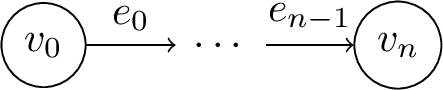 .
.
where \(v_0,\ldots,v_n\) are distinct nodes, \(e_0, \ldots, e_{n-1}\) are distinct edges (for \(n > 0\)), and each edge \(e_i\) has property \(e_i.k\). Let \(\psi^{\mathsf{E}}_{<}\) be \[\begin{array}{cl} & (x_s) \left(\big( (u)\overset{x}{\rightarrow}(z) \overset{y}{\rightarrow}(v) \overset{w}{\leftarrow} (z)\big) \langle x.k < y.k \rangle\right)^{1..\infty} \to (x_t)\\ + & (x_s)\to(x_t) \end{array}\] A pattern with output \(\psi_\Omega\) expresses a query \(Q\) on \(G\) if \(\left\llbracket\psi_\Omega\right\rrbracket_G = Q(G)\).
The pattern \(\big(\psi^{\mathsf{E}}_{<}\big)_{(x_s,x_t)}\) expresses \(Q^{\mathsf{E}}_{\uparrow}\) on annotated paths.
In the first disjunct, the forward edge \(\overset{y}{\rightarrow}\) serves as a look-ahead that enables checking whether the condition holds, and the backward edge \(\overset{w}{\leftarrow}\) enables us to continue constructing the path in the next iteration from the correct position \((z)\). The fact that the query operates on \(P_n\) ensures that the last edge to \(x_t\) does not violate the condition of the query as it was already traversed in the iterated subpattern. The second disjunct takes care of paths of length \(1\).
6.2 What cannot be expressed with patterns↩︎
To achieve expressibility of \(Q^{\mathsf{E}}_{\uparrow}\) in Proposition [prop:e60express] we made two strong assumptions: not only is the input of a very special shape (a directed path with forward edges), but also the pattern uses backwards edges; the latter would be natural for an oriented path (in which edges can go in either direction [31]), but looks rather unnatural in this setting. Thus, we ask ourselves whether \(Q^{\mathsf{E}}_{\uparrow}\) can be expressed in a natural way. In fact we can pose a more general question about queries \(Q^{\mathsf{E}}_w\) for arbitrary order motifs; in Section 6.1 we saw that on nodes, all order motifs can be expressed.
To formalize what we mean by “natural”, define one-way path patterns by a restriction of the grammar: \[\begin{align} \psi\;:=\;& (x) \;\mid\;\overset{x}{\rightarrow} \;\mid \; \psi_1 + \psi_2 \;\mid \; \psi^{n..m} \;\mid \;\psi_{\langle \theta \rangle} \;\mid\; \psi_1\, \psi_2 \end{align}\] where we require that \(\mathsf{FV}\left( \psi_1\right)\cap \mathsf{FV}\left(\psi_2\right) = \emptyset\) in \(\psi_1\, \psi_2\) (and variables \(x\), as before, are optional). The omission of backward edges \(\overset{x}{\leftarrow}\) in one-way patterns is quite intuitive. The restriction on variable sharing in concatenated patterns is because backward edges can be simulated by simply repeating variables, as done above in \(\psi^{\mathsf{E}}_{<}\).
If there is a natural way, easily found by programmers, of writing the \(Q^{\mathsf{E}}_{\uparrow}\) query in PGQ and GQL, one would expect it to be done without backward edges. Yet, this is not the case.
In fact, no order motif on edges can be captured by GQL and PGQ patterns.
Theorem 2. There is no order motif \(w\) such that \(Q^{\mathsf{E}}_w\) is expressible by a one-way path pattern query.
The inexpressibility of \(Q^{\mathsf{E}}_{\uparrow}\) is then an immediate corollary for \(w=\uparrow\).
This result is a direct consequence of a general pumping argument applied to annotated paths accepted by one-way patterns.
Theorem 3. For every one-way path pattern \(\psi\), if for every \(n\in \mathbb{N}\) there exists an annotated path \(p\) of length \(n\) accepted by \(\psi\) then there exists \(n_0\in \mathbb{N}\) such that for every annotated path \(p\) accepted by \(\psi\) with \(|p|>n_0\), the path \(p\) can be decomposed as \(p=p_1 p_2 p_3\), \(|p_2|>1\) and for every \(n\in \mathbb{N}\), the annotated path \(p_1 p_2^{n+1}p_3\) is also accepted by \(\psi\).
Note that in the newly constructed path with repetitions, we assign new ids to the different occurrences of the elements in \(p_2\), while keeping the data (annotations) unchanged. The idea behind the proof is as follows: Since, by definition, there are infinitely many annotated paths that conform to \(\psi\), it must exhibit unbounded repetition. However, because the semantics disregard variables that occur within unbounded repetitions, the transfer of information between iterations is limited. This restriction allows us to repeat parts of the annotated path while preserving the same semantics and, consequently, still conforming to \(\psi\).
We can derive a further corollary of this theorem that reinforces the intuition that GQL and PGQ patterns are incapable of capturing data values along a path “as a whole.”
A canonical example of such a condition is checking whether all values of a specific property of nodes or edges along a path are distinct. Formally, we define:
- \(Q^{\mathsf{N}}_{\neq}\) returns pairs \((u_0,u_n)\) of nodes such that there is path \(\textsf{path}(u_0,e_1,u_1,\ldots,e_n,u_n)\) so that \(u_i.k \neq u_j.k\) for all \(0 \leq i < j \leq n\).
and \(Q^{\mathsf{E}}_{\neq}\) is defined likewise but for edges in place of nodes. One-way path patterns do not have enough power to express such queries.
Corollary 2. No one-way path pattern expresses \(Q^{\mathsf{N}}_{\neq}\) nor \(Q^{\mathsf{E}}_{\neq}\).
6.3 What cannot be expressed in full GQL↩︎
Having examined the expressiveness of patterns, we now look at the entire query languages Core GQL and Core PGQ and compare them with recursive SQL and linear Datalog. Recursive SQL is a good comparison target as the most natural relational language into which graph queries involving pattern with arbitrary length paths are translated [32], [33]. The theoretical basis for recursive SQL common table expressions is linear Datalog, i.e., the fragment of Datalog in which definitions can refer to recursively defined predicates at most once. This is precisely the restriction of recursive SQL: a recursively defined table can appear at most once in .
Of course recursive SQL can be enormously powerful: as already mentioned, combining recursion and arithmetic/aggregates one can simulate Turing machines [34]. Thus, to make the comparison fair, we look at positive recursive SQL: this is the fragment of recursive SQL where subqueries can only define equi-joins. In other words, they only use conjunctions of equalities in . Such a language just adds recursion on top of unions of conjunctive queries, and ensures termination and tractable data complexity [35]. We show that even these simple fragments of SQL and Datalog can express queries that Core GQL and PGQ cannot define.
At the end of the section, we explain why this is quite surprising in view of what we know about Core GQL and PGQ: complexity-theoretic considerations strongly suggest these should define all queries from linear Datalog, and yet this is not the case due to subtle deficiencies in the language design, which we outline in Section 8.
To talk about expressing property graph queries in relational languages, we must represent graphs as relations. There are many possibilities, and it does not matter (for showing Theorem 4) which one we choose, as these different representations are inter-definable by means of unions of select-project-join queries. Since graphs in the separating example have labels and do not have property values, we use an encoding consisting of unary relations \(N_\ell\) storing \(\ell\)-labeled nodes, and binary relations \(E_\ell\) storing pairs of nodes \((n_1,n_2)\) with an \(\ell\)-labeled edge between them.
To sketch the idea of the separating query, we define dataless paths as graphs \(G_n\), \(n > 0\), with nodes \(v_0,\ldots,v_n\), edges \((v_0,v_1), \;(v_1,v_2), \ldots, (v_{n-1},v_n)\), where \(v_0\) has label \(\mathit{min\_elt}\) and \(v_n\) has label \(\mathit{max\_elt}\). The separating query asks: is \(n\) a power of 2?
The inexpressibility proof of this is based on showing that GQL queries can only define Presburger properties of lengths of dataless paths, by translating Core GQL queries on such paths into formulae of Presburger Arithmetic (i.e., the first-order theory of \(\langle \mathbb{N}, +, <\rangle\)). Therefore the only definable properties of lengths are semilinear sets [36]. Semi-linear subsets of \(\mathbb{N}\) are known to be ultimately periodic: that is, for such a set \(S\subseteq \mathbb{N}\), there exists a threshold \(t\) and a period \(p\) such that \(n\in S\) if and only if \(n+p\in S\), as long as \(n>t\). Clearly the set \(\{2^k \mid k \in \mathbb{N}\}\) is not such.
The query can be expressed in positive recursive SQL:
WITH RECURSIVE ADD(A, B, C) AS ( (SELECT P.A, MIN_ELT.A AS B, P.A AS C FROM P, MIN_ELT) UNION (SELECT MIN_ELT.A, P.A AS B, P.A AS C FROM P, MIN_ELT) UNION (SELECT ADD.A, P1.B, P2.B AS C FROM ADD, P P1, P P2 WHERE ADD.B=P1.A AND ADD.C=P2.A) ), POW2(A, B) AS ( (SELECT P2.A, P2.B FROM MIN_ELT M, P P1, P P2 WHERE M.A=P1.A AND P1.B=P2.A) UNION (SELECT P.B AS A, ADD.C AS B FROM POW2, ADD, P WHERE POW2.A=P.A AND ADD.A=POW2.B AND ADD.B=POW2.B) ) (SELECT ‘YES’ FROM POW2, MAX_ELT WHERE POW2.B=MAX_ELT.A)
The path is given by a binary relation P containing pairs \((v_i,v_{i+1})\) while minimal/maximal elements \(v_0\) and \(v_n\) are given by
unary relations MIN_ELT and MAX_ELT. The first common table expression defines a ternary relation ADD with tuples \((v_i,v_j,v_k)\) such that \(i+j=k\). If \(v_i\) is in MIN_ELT, then \((v_i,v_j,v_j)\) and \((v_j,v_i,v_j)\) are in ADD for all
\(j\) (the basis of recursion), and if \((v_i,v_j,v_k)\) is in ADD then so is \((v_{i+1},v_j,v_{k+1})\) (the recursive step). After that
POW2 builds a relation with tuples \((v_i,v_j)\) for \(j = 2^i\). Indeed, if \((v_i,v_j)\) is in POW2, then so is \((v_{i+1},v_k)\) for \(k=2\cdot j\), which is tested by \((v_j,v_j,v_k)\in\texttt{ADD}\). The length of the path is a power of 2 if the second projection of
POW2 contains MAX_ELT.
Note that ADD is defined by a linear Datalog program and POW2 is defined by a linear Datalog program that uses ADD as EDB. Hence, the entire query is defined by a piece-wise linear program (where already defined
predicates can be used as if they were EDBs). It is known that such programs can be expressed in linear Datalog [37].
6.3.0.1 Complexity-theoretic considerations.
We now explain why the inexpressibility result is quite unexpected. Note that all graph pattern languages can express the reachability query. It is complete for the complexity class \(\mathrm{\small NLogSpace}\) via first-order reductions [38]: an extension of first-order logic with the reachability predicate capturtes precisely all \(\mathrm{\small NLogSpace}\)queries. Since GQL and PGQ can emulate relational algebra (and thus first-order logic) over pattern matching results, it appears that they should be able to express all \(\mathrm{\small NLogSpace}\)queries. In fact graph query languages expressing all \(\mathrm{\small NLogSpace}\)queries have been known for a long time, starting with GraphLog crpq?, which introduced the ubiquitous notion of CRPQs.
However, Theorem 4 not only refutes the complexity-based intuition, but in fact the separating query has an even lower \(\mathrm{\small DLogSpace}\) complexity. Indeed, one can traverse the dataless path graph while maintaining the counter that needs a logarithmic number of bits. This limitation highlights a deficiency of the language design: despite having access to reachability and full power of first-order logic on top of it, Core GQL and PGQ fall short of a declarative language that is first-order logic with the reachability predicate. The reason for this deficiency, that should ideally be addressed in future revisions of the standards, is discussed below in Section 8.
7 Limitations of Patterns: an experimental investigation↩︎
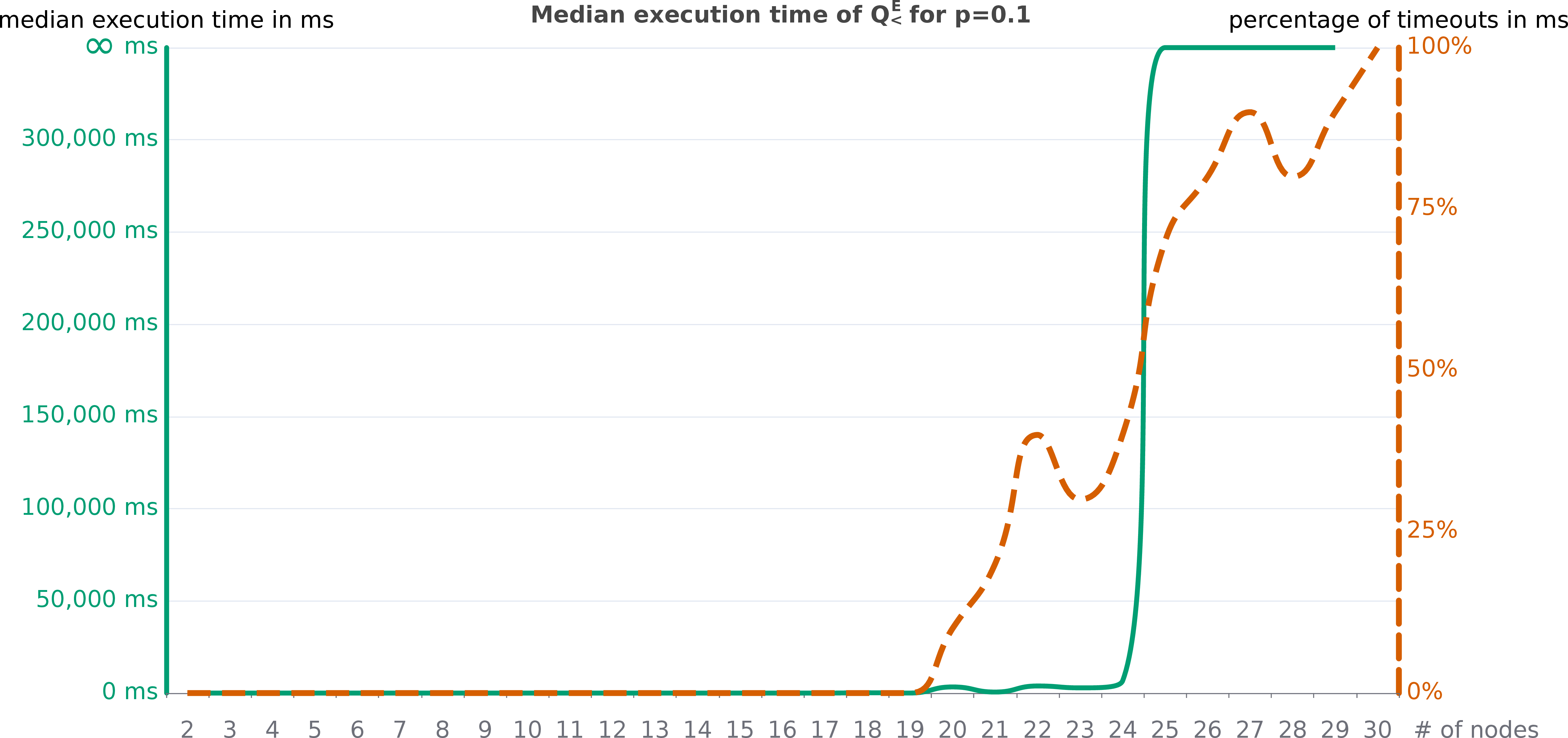
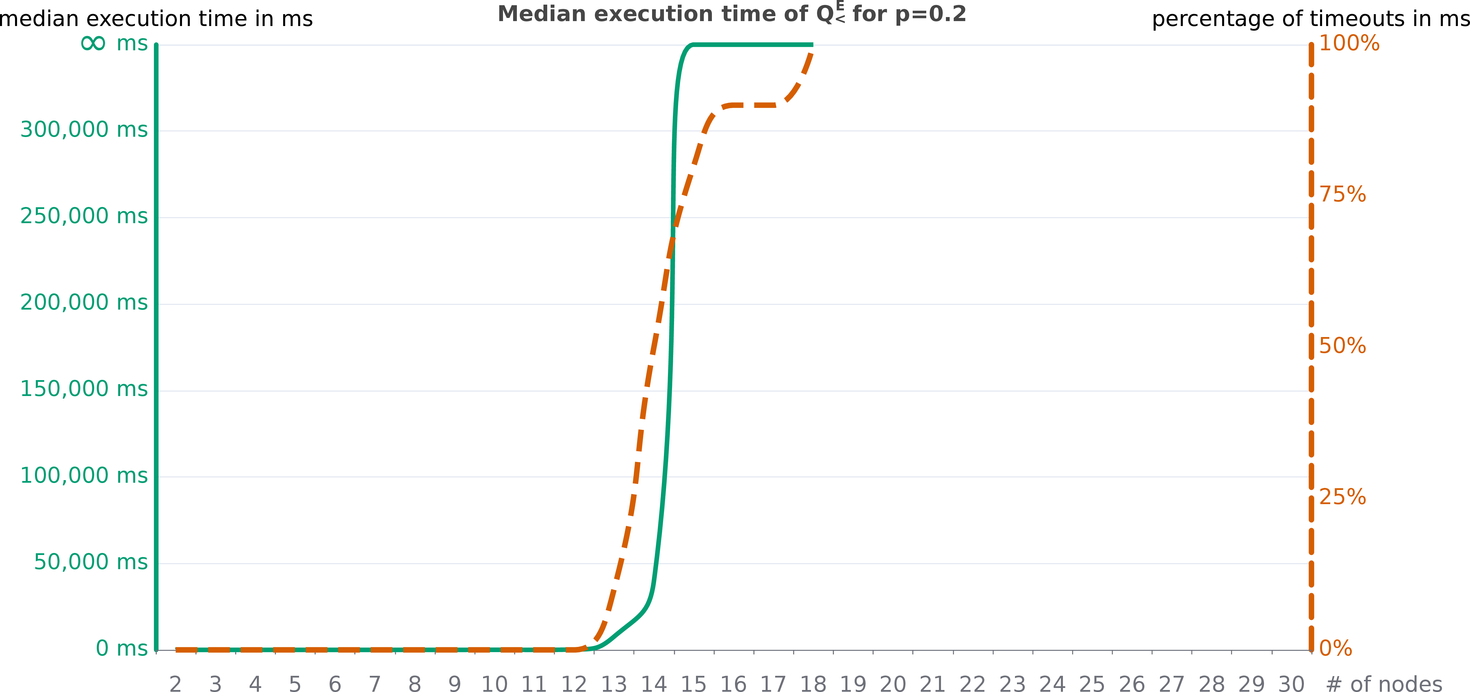
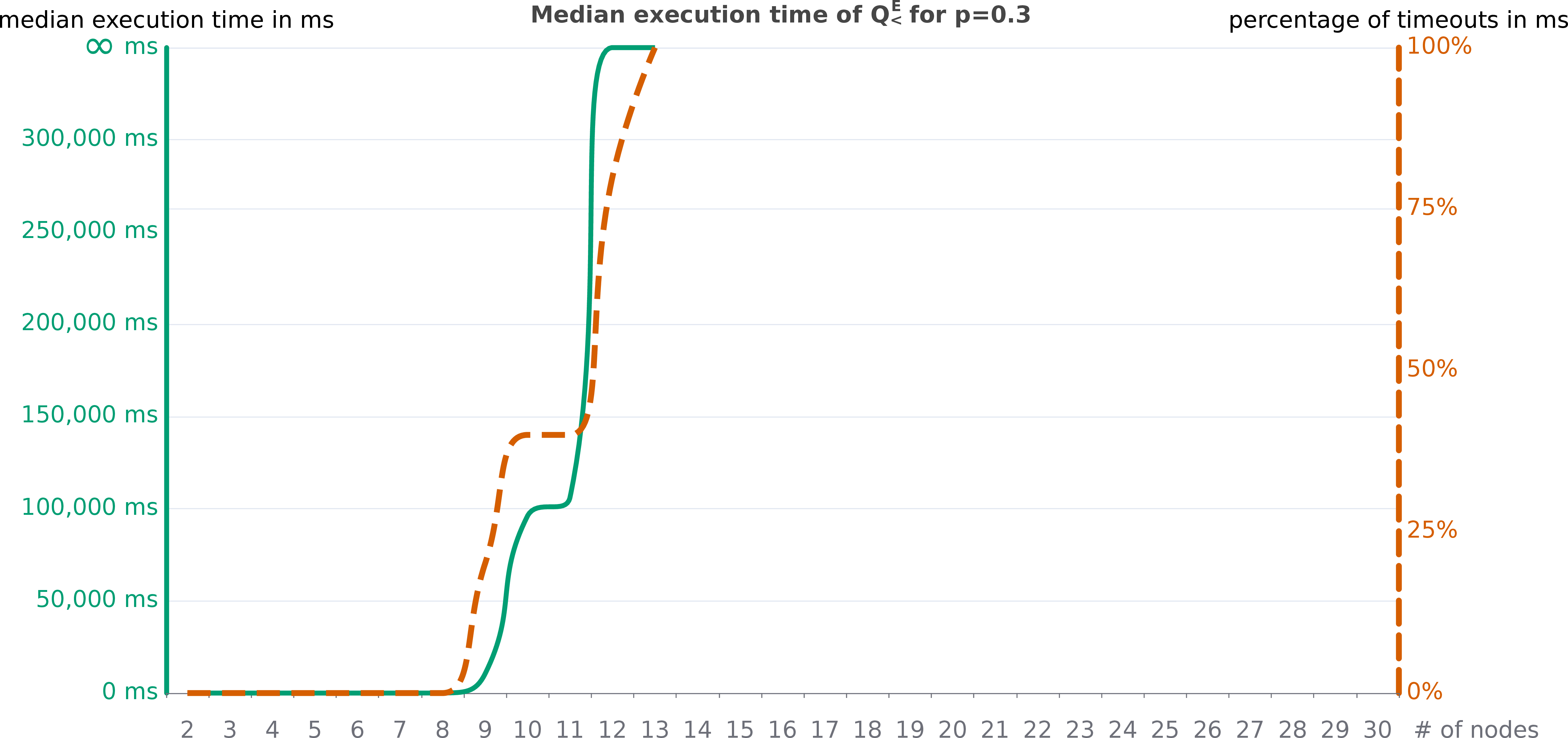
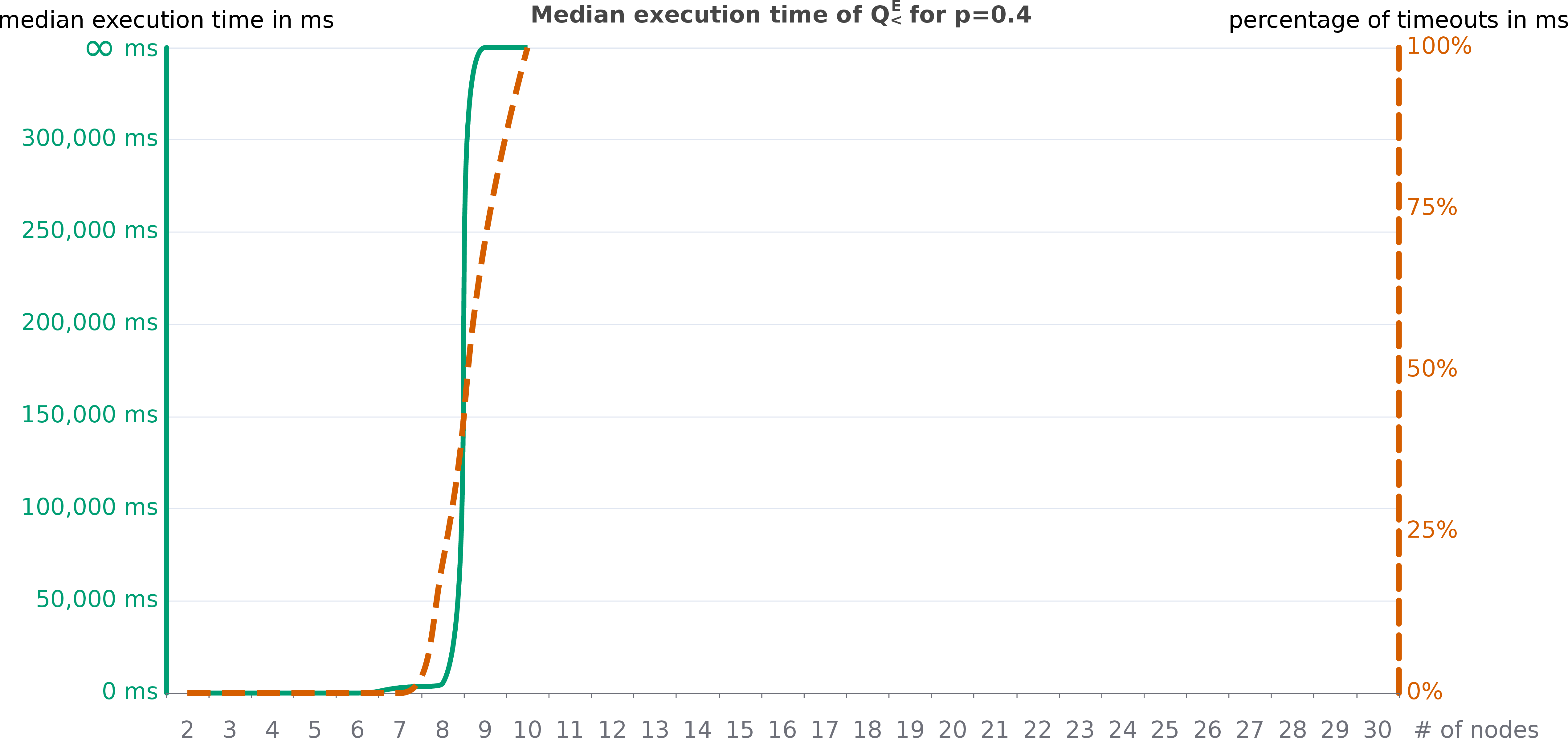
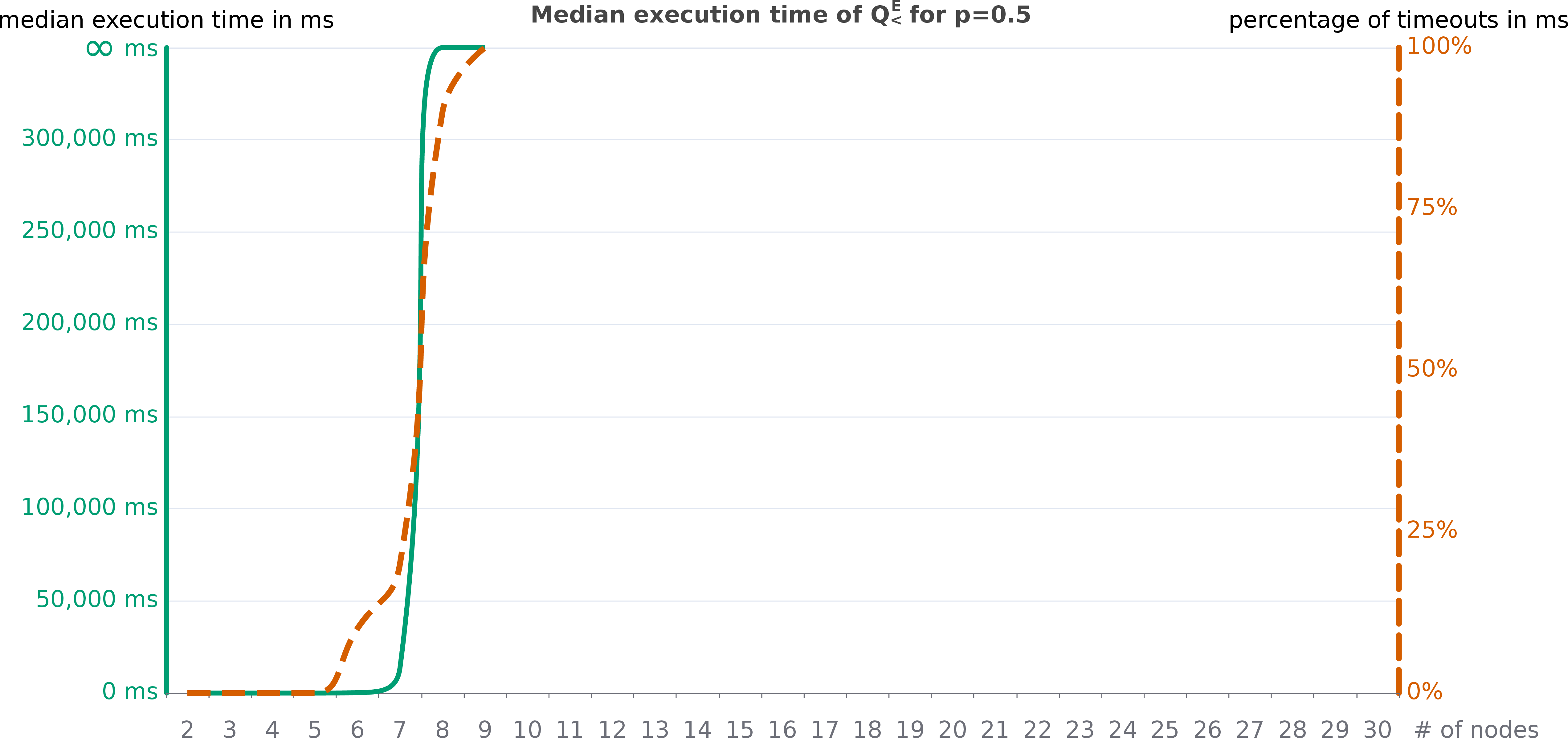
Figure 4: Timeouts and median running time of Neo4j for \(Q^{\mathsf{E}}_{\uparrow}\). a — \(p=0.1\), b — \(p=0.2\), c — \(p=0.3\), d — \(p=0.4\), e — \(p=0.5\)
We have shown that many queries tracing changes in property values of edges cannot be expressed in Core GQL and PGQ, among them the simple query \(Q^{\mathsf{E}}_{\uparrow}\) that generated significant interest in the GQL standardization committee of ISO [16], [17]. Of course real-life languages have more expressiveness than their theoretical counterparts, and thus real-life GQL, SQL/PGQ, and also Cypher can express this query. However, they do so in a rather convoluted way. We now show experimentally that this way of expressing simple graph queries has no realistic chance to work, as it generates enormous (exponential size) intermediate results, and the query would not terminate even on tiny graphs.
The idea of expressing \(Q^{\mathsf{E}}_{\uparrow}\) is that its complement is easily definable in Core GQL. In GQL, PGQ, and Cypher, paths can be named and output. This is an advanced feature that we omitted in our core language: since paths are represented as lists, it results in non-flat outputs.
The complement of \(Q^{\mathsf{E}}_{\uparrow}\) is expressed by the pattern \(\psi^\neg\):
(v1)->*(-[x]-> -[y]-> WHERE x.k>=y.k)->*(v2)
testing for a pair of consecutive edges that break the increasing motif; it can also be expressed by CoreGQL as \[\psi^\neg :=(v_1) \to^{0..\infty} \big(\;() \overset{x}{\rightarrow} () \overset{y}{\rightarrow} ()\;\big)\langle x.k \geq y.k\rangle \to^{0..\infty}(v_2)\,.\]
Thus, the query below
MATCH p = (v1) ->* (v2) RETURN v1, v2, p EXCEPT MATCH p=(*\(\varphi^\neg\)*) RETURN v1, v2, p
finds all nodes \(v_1, v_2\) and path \(p\) between them satisfying \(Q^{\mathsf{E}}_{\uparrow}\). The mere fact of expressing something does not yet mean it will work – for example, despite SQL having the capability to simulate Turing machines, we do not expect it to perform well with complex graph algorithms. Likewise here, the first subquery enumerates paths between two different nodes, and even the number of simple paths between two nodes in a graph can grow as fast as \(O(n!/n^2)\).
We now show experimentally that queries of this kind have no chance to work even on very small graphs. A small obstacle is that there is not yet any available implementation of GQL, and Cypher, the closest language, chose not to have \(\text{\normalfont\small\renewcommand{\ttdefault}{pcr}\ttfamily\bfseries\color{darkblue} EXCEPT}\). However, there is a way around it in Cypher by using list functions that can detect the violation of the “value in edges increases” condition:
MATCH p=()-[*2..]->() WITH p, reduce(acc=relationships(p)[0].val, v in relationships(p) | CASE WHEN acc=-1 THEN -1 WHEN v.val>=acc THEN v.val ELSE -1 END) AS inc WHERE NOT inc = -1 RETURN p
We then tested its median running time in Neo4j2, as well as the percentage of queries that time out (the timeout is set at 300 seconds). When more than 50% of queries time out, the median is shown as \(\infty\)ms. Otherwise the running time is computed as the median over 10 different graphs, with 1 run per graph (and an additional run 0 to generate the appropriate indices).
The graphs on which we tested the query are the random graphs \(G(n,p)\) [39] on \(n\) nodes where an edge exists between two nodes with probability \(p\). We considered values \(p\) between 0.1 and 0.5, with the step 0.1. As for data values in edges, they are also randomly generated, between 0 and 100. The reason we used this simple model of synthetic property graphs is that it very convincingly demonstrates that the above implementation of \(Q^{\mathsf{E}}_{\uparrow}\) has no chance to work in practice. Even with the smallest probability of 0.1, with a mere 24 nodes timeout was observed in more than 50% of all cases, and with just 30 nodes in all cases. As the probability \(p\) increases (meaning that there are more edges in the graph, and thus the number of paths increases), the cutoff for everything-times-out dropped to fewer than 10 nodes!
We add two notes here. Queries \(Q^{\mathsf{N}}_{\neq}\) and \(Q^{\mathsf{E}}_{\neq}\) can be similarly expressed, with the bottleneck query matching all paths being identical to the above, hence resulting in a very similar behavior. But behavior is not observed with \(Q^{\mathsf{N}}_{\uparrow}\) as it can be expressed directly with Cypher and GQL pattern matching, without having to find an exponential number of paths.

7.0.0.1 Other systems
Even though it appears that bypassing expressivity bounds by generating exponentially many queries should not have a chance to work (as our Neo4j tests confirm), we wanted to completely exclude the possibility that this behavior could be due to one specific implementation. Thus, to confirm the above results, we ran the same tests on two other systems: Memgraph, a graph-only database that uses Cypher as its query language, and DuckDB, a relational database that implements SQL/PGQ as an extension [27].
The results confirm that the problem is the way the query is written rather than a particular implementation. In fact, the limits of Neo4j and Memgraph are almost identical as shown in Fig. 5 which reports numbers of nodes at which 50% and 100% of runs timeout.
However, it must be noted that for the configurations that do not timeout, the performance of Memgraph appears to be much more efficient than that of Neo4j, with almost all test cases taking less than 1 ms. This might be explained by the fact that the timing procedures are different for the two systems as Memgraph does not make query execution time available to the driver.
The performance of DuckDB was tested using the SQL/PGQ query below; it first finds the shortest paths in the graph using the PGQ pattern matching syntax (the inner query), then checks, in SQL, that the edge weights appear in sorted order (the outer query).
WITH q1 AS (SELECT *, unnest(path_edges) AS e_id FROM GRAPH_TABLE (testgraph MATCH p = ANY SHORTEST (n1:N)-[e:E]->2,(n2:N) COLUMNS (edges(p) AS path_edges) ), LATERAL (SELECT edges.weight, edges.row_id FROM edges) ) SELECT path_edges, array_agg(weight) AS weights FROM q1 WHERE e_id=row_id GROUP BY path_edges HAVING ARRAY_AGG(weight) = ARRAY_SORT(ARRAY_AGG(weight));
While the results for DuckDB appear to be better than for native graph systems (it can handle 164 nodes with the lowest probability \(p=0.1\) before running out of memory), there is a simple explanation for it: the difference in path semantics. The only path semantics available for repeated patterns in DuckDB is shortest path, whereas the only one available in Neo4j and Memgraph is trail, which matches paths that do not go through the same edge twice. In most graphs there are significantly more trails than shortest paths between any given nodes, hence the number of candidate paths to be checked is much higher for Neo4j and Memgraph than for DuckDB. Even with this, however, the way of bypassing expressivity bounds by generating a large number of paths can only handle very small graphs, not even reaching 200 nodes.
8 What we learned about language design problems↩︎
A common way of enhancing the capabilities of query languages is: (1) an initial design is produced; (2) user-demanded queries that are not expressible in this initial design are identified; (3) their inexpressibility is formally confirmed; (4) language deficiencies that led to (3) are identified; (5) these deficiencies are fixed. Note that (5) is often an iterative process that involves a deep analysis of possible language design enhancements. Returning to the example of recursive queries in SQL, note that while it was quite clear that programmers cannot write queries such as transitive closure, it took a significant effort to confirm this formally. Subsequently hundreds of papers analyzed the expressiveness and complexity of datalog and fixed-point extensions of relational calculus, until the linear datalog approach was adopted by the SQL standard.
Where does this workflow put us with respect to the new graph standards, SQL/PGQ and GQL? Prior to this paper we were at stage (2); the results of this paper complete step (3) and put us at the beginning of stage (4). Thus, in this last section we outline further developments as we envision them now: what language deficiencies cause limited expressiveness, and how they could be addressed.
The main limitation of current graph query languages is that they lack compositionality. They are essentially graphs-to-relations languages, as opposed to graph-to-graph languages (though some ad hoc functionalities exist for viewing relational outputs into graphs, such as the Neo4j browser or its data science library facilities [40] that can extract graphs from relations for analytics tasks; also the study of graph views is in its infancy [41]). The lack of compositionality also manifests itself in the information flow in graph query languages. It happens in one direction, from graphs to relations: patterns turn graphs into relations, but there are no natural ways of going in the other direction, and use results of relational operations of either \(\mathsf{RA}\) or \(\mathsf{LCRA}\) to create new graphs. Of course real-life languages with their extended functionalities provide such ways (e.g., via libraries as mentioned above, or by writing data and using it to create new graph views in PGQ) – but the main point is that these lie outside the realm of a declarative query language.
With the understanding of causes of limitations, the focus needs to be shifted to ways to remedy those, i.e., step (5) above. If the story of SQL is any indication, this will require a considerable research effort. Still, we can outline what we think are possible approaches to fixing the non-compositionality issues.
8.0.0.1 Pattern matching restricted to matched paths
While graph-to-graph languages are the ultimate long-term goal, in the short term some of non-compositionality can be fixed by letting pattern matching operate on previously matched patterns. We explain this idea by the query \(Q^{\mathsf{E}}_{\uparrow}\). To find such paths from \(\ell_1\)-labeled nodes to \(\ell_2\)-labeled nodes, we can first match paths from \(\ell_1\)-nodes to \(\ell_2\)-nodes and then exclude those where the “increasing value in edges” condition is violated. Specifically, we start with the pattern \(\psi:=(x) \to^{1..\infty} (y) \langle{\ell_1(x) \wedge \ell_2(y)}\rangle\) and then create a new pattern \[\label{eq-for-concl} \psi\;| \;\neg\exists(\overset{u}{\to} \;() \;\overset{v}{\to}\langle u.k \geq v.k\rangle)\tag{1}\] The pipe operator \(|\) means that the pattern \(\overset{u}{\to} () \overset{v}{\to}\langle u.k \geq v.k\rangle\) is evaluated on the result of the match of pattern \(\psi\), and the condition \(\neg\exists\) says that there are no matches for it. This will ensure that in the match for \(\psi\) there are no consecutive edges for which the value of their property does not increase.
8.0.0.2 Constructing graph elements from tables
In current graph languages the flow of information is in the direction from graph to constructed relations. What if we could reverse it as well and construct new graph elements from relations? As an example of this, suppose we could construct new nodes with label old_edge whose ids are edge ids in a graph \(G\), and a new edge with a lable new_edge which connects two such nodes coming from edges \(e_1\) and \(e_2\) of \(G\) if the target of \(e_1\) is the source of \(e_2\). Then \[(x) \big( (u) \overset{e}{\to} (v)\langle u.k<v.k \wedge \textit{new\_edge}(e)\rangle \big) (y)\] (i.e., \(Q^{\mathsf{N}}_{\uparrow}\) on the constructed graph) expresses \(Q^{\mathsf{E}}_{\uparrow}\) on \(G\). This powerful idea was already present in an early theoretical language of crpq? but never properly explored in the context of practical graph languages.
Language design is a delicate process in which the right balance must be struck between expressivity and complexity. It is not simple “add these features”; much new research is required as they come with complexity consequences. To give one example, in (1 ) replace \(\overset{u}{\to} () \overset{v}{\to}\langle u.k \geq v.k\rangle\) with \((u) \to^{1..\infty} (v)\langle u.k = v.k\rangle\). This results in query \(Q^{\mathsf{N}}_{\neq}\) known to be NP-hard in data complexity [10]. Thus, such extensions are very sensitive to small syntactic changes. This however should simply be viewed as an invitation to start a research investigation into extensions of GQL and PGQ that allow desirable queries without unmanageable computational overhead. Once again, the past history of SQL tells us that such research could be very productive and have a great influence on the language.
Acknowledgments↩︎
This research was supported by ANR-21-CE48-0015 Project VeriGraph, a grant from RelationalAI to IRIF, Poland’s National Science Centre grant 2018/30/E/ST6/00042, and Israel Science Foundation grant 2355/24.
9 Proof of theorem [prop:SLRA-vs-LRA]↩︎
At first, observe that simple linear clauses (without \(\{\mathcal{Q}\}\)) can only express conjunctive queries, as their semantics applies operations \(\bowtie, \pi, \sigma\) and renaming to base relations. Hence, queries of sLCRA are Boolean combinations of conjunctive queries, known as BCCQs. While it appears to be folklore that BCCQs are strictly contained in first-order logic, we were unable to find the simple proof explicitly stated in the literature, hence we offer ohe here.
Consider a vocabulary of a single unary predicate \(U\) and databases \(\mathcal{D}_1\) and \(\mathcal{D}_2\) such that \(\mathcal{D}_1(U) = \{a_1\}\) and \(\mathcal{D}_2(U) = \{a_1,a_2\}\) for two different constants \(a_1\) and \(a_2\). Since \(\mathcal{D}_1\) and \(\mathcal{D}_2\) are homomorphically equivalent, they agree on all conjunctive queries, and therefore on all BCCQs, but they do not agree on first-order (and hence \(\mathsf{RA}\)) query that checks if relation \(U\) has exactly one element.
10 Proof of theorem 1↩︎
We first prove that \(\mathsf{RA}(\mathbf{S})\) is subsumed by \(\mathsf{LCRA}(\mathbf{S})\). Let \(Q\) be a query in \(\mathsf{RA}(\mathbf{S})\). We show that there exists an equivalent query \(Q^{\mathsf{LCRA}}\) in \(\mathsf{LCRA}(\mathbf{S})\), i.e. such that for every database \(\mathcal{D}\) over \(\mathbf{S}\) it holds that \(\left\llbracket Q\right\rrbracket_{\mathcal{D}} = \left\llbracket Q_L\right\rrbracket_{\mathcal{D}}\) by induction on the structure of \(Q\).
(base case) If \(Q = R\) then \(Q_L = S\) where \(S = \{R\}\)
If \(Q = \psi_{\bar{A}} (Q')\) and \(Q'_L\) is the LRA query equivalent to \(Q'\) then \(Q_L = Q'_L~\pi_{\bar{A}}\)
If \(Q = \sigma_{\theta}(Q')\) and \(Q'_L\) is the LRA query equivalent to \(Q'\) then \(Q_L = Q'_L ~ \sigma_{\theta}\)
If \(Q = \rho_{\bar{A} \rightarrow \bar {B}}(Q')\) and and \(Q'_L\) is the LRA query equivalent to \(Q'\) then \(Q_L = Q'_L~\rho_{\bar{A} \rightarrow \bar {B}}\)
For the three following cases, \(Q'\) (resp. \(Q''\)) is systematically translated as \(\{Q'_L\}\) (resp. \(\{Q_L''\}\))
If \(Q = Q' \cup Q''\) and \(Q'_L\) (resp. \(Q''_L\)) is the LRA query equivalent to \(Q'\) (resp. \(Q''\)) then \(Q_L = \{Q'_L\} \cup \{Q''_L\}\)
If \(Q = Q' \setminus Q''\) and \(Q'_L\) (resp. \(Q''_L\)) is the LRA query equivalent to \(Q'\) (resp. \(Q''\)) then \(Q_L = \{Q'_L\} \setminus \{Q''_L\}\)
If \(Q = Q' \bowtie Q''\) and \(Q'_L\) (resp. \(Q''_L\)) is the LRA query equivalent to \(Q'\) (resp. \(Q''\)) then \(Q_L = \{Q'_L\} \{Q''_L\}\) as, by definition of RA, it must be that \(\mathsf{attr}(Q') \cap \mathsf{attr}(Q'') = \emptyset\)
We now prove that \(\mathsf{LCRA}(\mathbf{S})\) is subsumed by \(\mathsf{RA}(\mathbf{S})\). Let \(Q\) be a query in \(\mathsf{LCRA}(\mathbf{S})\). We show that there exists a query \(Q^{RA} \in \mathsf{RA}(\mathbf{S})\) such that for every database \(\mathcal{D}\) over \(\mathbf{S}\) it holds that \(\left\llbracket Q\right\rrbracket_{\mathcal{D}} = \left\llbracket Q^{RA}\right\rrbracket_{\mathcal{D}}\) by induction on the structure of \(Q\).
We start with the linear clauses. Since their structure is not tree-shaped, but indeed linear, the query must be parsed from left to right, while the equivalent \(\mathsf{RA}\) query will be built bottom-up. Let \(C = c_0, \ldots, c_n\) be a linear clause in \(\mathsf{LCRA}(\mathbf{S})\). We build the induction on the number of clauses of \(C\).
(base case) If \(n=1\) and \(C\) is an instance of the \(S\) rule, i.e. \(C = R\) for some \(R\) then the \(\mathsf{RA}\) query equivalent to \(C\) is \(R\)
(base case) If \(n=1\) and \(C\) is one of \(\pi_{\bar{A}}, \sigma_{\theta}\) or \(\rho_{\bar{A} \rightarrow \bar {B}}\) then the \(\mathsf{RA}\) query equivalent to \(C\) is \(I_{\emptyset}\) (the empty tuple relation)
(base case) If \(n=1\) and is \(C\) is an instance of the \(\{Q\}\) rule, then the \(\mathsf{RA}\) query equivalent to \(C\) is the one equivalent to \(Q\) (see induction for queries below)
For the inductive cases, let \(C_i^{RA}\) be the \(\mathsf{RA}\) query such that \(\left\llbracket c_0, \ldots, c_i\right\rrbracket = \left\llbracket C_i^{RA}\right\rrbracket\)
If \(n > 1\) and \(c_{i+1}\) is an instance of the \(S\) rule, i.e. \(c_{i+1} = R\), then \(C_{i+1}^{RA} = C_i^{RA} \bowtie R\)
If \(n > 1\) and \(c_{i+1} = \pi_{\bar{A}}\), then \(C_{i+1}^{RA} = \pi_{\bar{A}} (C_i^{RA})\)
If \(n > 1\) and \(c_{i+1} = \sigma_{\theta}\), then \(C_{i+1}^{RA} = \sigma_{\theta} (C_i^{RA})\)
If \(n > 1\) and \(c_{i+1} = \rho_{\bar{A} \rightarrow \bar{B}}\), then \(C_{i+1}^{RA} = \rho_{\bar{A} \rightarrow \bar{B}} (C_i^{RA})\)
If \(n > 1\), \(c_{i+1} = \{Q\}\) and \(C_Q^{RA}\) is the \(\mathsf{RA}\) query equivalent to \(Q\), then \(C_{i+1} = C_i^{RA} \bowtie C_Q^{RA}\)
We now treat the queries. Let \(Q\) be an \(\mathsf{LCRA}\) query. We build the induction on the structure of \(Q\).
(base case) If \(Q = L\) then the \(\mathsf{RA}\) query equivalent to \(Q\) is the one equivalent to \(L\) (see above for induction on linear clauses).
If \(Q = Q_1 \cap Q_2\) and \(Q_1^{RA}\) (resp. \(Q_2^{RA}\)) is the \(\mathsf{RA}\) query equivalent to \(Q_1\) (resp. \(Q_2\)) then the \(\mathsf{RA}\) query equivalent to \(Q\) is \(Q_1^{RA} \cap Q_2^{RA}\)
If \(Q = Q_1 \cup Q_2\) and \(Q_1^{RA}\) (resp. \(Q_2^{RA}\)) is the \(\mathsf{RA}\) query equivalent to \(Q_1\) (resp. \(Q_2\)) then the \(\mathsf{RA}\) query equivalent to \(Q\) is \(Q_1^{RA} \cup Q_2^{RA}\)
If \(Q = Q_1 \setminus Q_2\) and \(Q_1^{RA}\) (resp. \(Q_2^{RA}\)) is the \(\mathsf{RA}\) query equivalent to \(Q_1\) (resp. \(Q_2\)) then the \(\mathsf{RA}\) query equivalent to \(Q\) is \(Q_1^{RA} \setminus Q_2^{RA}\)
11 Proof of Theorem 2↩︎
For an annotated path \(p\), we define \(w_p\) as the sequence \(e_0.k\cdots e_{n-1}.k\).
Lemma 1. For every one-way path pattern \(\psi\) and annotated paths \(p,p'\) with \(w_{p'}=w_p\), if \((p,\mu)\in \left\llbracket\psi\right\rrbracket_{p}\) then there is \(\mu'\) such that \((p',\mu')\in \left\llbracket\psi\right\rrbracket_{p'}\).
Proof. Assume that \((p,\mu)\in \left\llbracket\psi\right\rrbracket_{p}\). Let us denote \(p\) by
Figure 6:  .
.
and \(p'\) by
Figure 7: 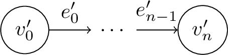 .
.
(Note that they have the same length since \(w_p = w_{p'}\).) We denote by \(f\) the mapping defined by \(f(v_i) :=v'_i\) for \(0\le i \le n\), and \(f(e_i) = e'_i\) for \(0 \le i \le n-1\). We then define \(\mu'\) by setting \(\mathsf{dom}(\mu') = \mathsf{dom}(\mu)\) and \(\mu'(x) :=f(\mu(x))\). It can be shown by induction on \(\psi\) that if \((p,\mu)\in \left\llbracket\psi\right\rrbracket_{p}\) then \((p',\mu')\in \left\llbracket\psi\right\rrbracket_{p'}\). ◻
For two annotated paths \(p:=\)
Figure 8: 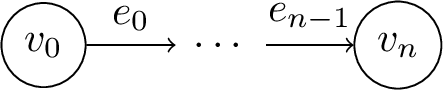 .
.
and \(p':=\)
Figure 9: 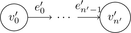 .
.
we use \({p'}\sqsubseteq p\) to denote that \(p'\) is contained within \(p\). Formally, \({p'}\sqsubseteq p\) if there is \(j\) such that \(v'_0 = v_j, \ldots, v'_{n'} = v_{j+n'}\), and \(e'_0 = e_j,\ldots , e'_{n'-1} = e_{j+n'-1}\).
Lemma 2. For every one-way path pattern \(\psi\) and annotated paths \(p,p'\) where \({p'}\sqsubseteq p\),
if there is \(\mu\) such that \((p',\mu)\in \left\llbracket\psi\right\rrbracket_p\) then \((p',\mu)\in \left\llbracket\psi\right\rrbracket_{p'}\)
\(\left\llbracket\psi\right\rrbracket_{p'} \subseteq \left\llbracket\psi\right\rrbracket_p\)
Proof. We use the same notation as above and show the claim by a mutual induction on \(\psi\). We skip the induction basis since it is trivial, and refer to the following interesting case in the induction step:
\(\psi= \psi_1\psi_2\) and assume \((p',\mu) \in \left\llbracket\psi_1\psi_2\right\rrbracket_p\). By definition, there are \(p_1,p_2,\mu_1,\mu_2\) such that \(p' = p_1p_2\), \((p_1,\mu_1) \in \left\llbracket\psi_1\right\rrbracket_p, (p_2,\mu_2) \in \left\llbracket\psi_2\right\rrbracket_p\), \(\mu_1\sim \mu_2\), and \(p_2\) concatenates to \(p_1\). Notice that \(p_1,p_2\sqsubseteq p'\), and hence also \(p_1p_2 \sqsubseteq p'\). By applying induction hypothesis \((1)\), we get \((p_1,\mu_1) \in \left\llbracket\psi_1\right\rrbracket_{p_1}, (p_2,\mu_2) \in \left\llbracket\psi_2\right\rrbracket_{p_2}\). By applying induction hypothesis \((2)\) we get \((p_1,\mu_1) \in \left\llbracket\psi_1\right\rrbracket_{p_1p_2}, (p_2,\mu_2) \in \left\llbracket\psi_2\right\rrbracket_{p_1p_2}\). This allows us to conclude that, by definition, \((p_1p_2,\mu_1\bowtie\mu_2) \in \left\llbracket\psi_1\psi_2\right\rrbracket_{p_1p_2}\).
If \(\psi= \psi_1 \psi_2\) then \(\left\llbracket \psi_1 \psi_2\right\rrbracket_{p'} = \left\{ ({p_1\, p_2}, \mu_1\bowtie\mu_2 ) \,\middle| \begin{array}{l}(p_1,\mu_1)\in\left\llbracket\psi_1\right\rrbracket_{p'}, (p_2,\mu_2)\in\left\llbracket\psi_2\right\rrbracket_{p'},\\ \mu_1\sim \mu_2, p_2 \text{ concatenates to }p_1 \end{array} \right\}\). By induction hypothesis \((2)\), \(\left\llbracket\psi_1\right\rrbracket_{p'} \subseteq \left\llbracket\psi_1\right\rrbracket_{p}\) and \(\left\llbracket\psi_2\right\rrbracket_{p'} \subseteq \left\llbracket\psi_2\right\rrbracket_{p}\). Thus, \[\left\llbracket \psi_1 \psi_2\right\rrbracket_{p'} \subseteq \left\{ ({p_1\, p_2}, \mu_1\bowtie\mu_2 ) \,\middle| \begin{array}{l}(p_1,\mu_1)\in\left\llbracket\psi_1\right\rrbracket_{p}, (p_2,\mu_2)\in\left\llbracket\psi_2\right\rrbracket_{p},\\ \mu_1\sim \mu_2, p_2 \text{ concatenates to }p_1 \end{array} \right\}.\] By definition, \(\left\llbracket \psi_1 \psi_2\right\rrbracket_{p'} \subseteq \left\llbracket \psi_1 \psi_2\right\rrbracket_{p}\).
◻
Let \(\psi\) be a path pattern. We define \[\mathcal{L}(\psi) = \{w \mid \forall\,p: \left(w=w_p \rightarrow \exists\, \mu:(p,\mu )\in \left\llbracket\psi\right\rrbracket_{p} \right) \}\]
For concatenation, we have:
Lemma 3. For every one-way path patterns \(\psi_1,\psi_2\), the following equivalence holds: \(\mathcal{L}(\psi_1 \psi_2) = \mathcal{L}(\psi_1 )\mathcal{L}(\psi_2)\).
Proof. \(\subseteq\) direction: Assume \(w\in\mathcal{L}(\psi_1 \psi_2)\). By definition, for every \(p\) such that \(w=w_p\) there is \(\mu\) such that \((p,\mu) \in \left\llbracket\psi_1\psi_2\right\rrbracket_p\). In turn, by definition of \(\left\llbracket\psi_1\psi_2\right\rrbracket_p\) we can conclude that there are paths \(p_1,p_2\) such that \(p=p_1p_2\) and there are \(\mu_1,\mu_2\) for which \((p_1,\mu_1)\in \left\llbracket\psi_1\right\rrbracket_p\), \((p_2,\mu_2)\in \left\llbracket\psi_2\right\rrbracket_p\), and \(\mu_1\sim \mu_2\). We set \(w_1 = w_{p_1}\) and \(w_2 = w_{p_2}\). For \(p_1\) we already saw that there is a \(\mu_1\) such that \((p_1,\mu_1)\in \left\llbracket\psi_1\right\rrbracket_p\). Let \(p'\) be such that \(w_1 = w_{p_1} = w_{p'}\). By Lemma 1, we can conclude that there is \(\mu'\) such that \((p',\mu')\in\left\llbracket\psi_1\right\rrbracket_{p'}\). Hence, by definition \(w_1 \in \mathcal{L}(\psi_1)\). We can show similarly that \(w_2 \in \mathcal{L}(\psi_2)\), which completes this direction.
\(\supseteq\) direction: Assume that \(w\in \mathcal{L}(\psi_1 )\mathcal{L}(\psi_2)\). That is, there are \(w_1, w_2\) such that \(w= w_1w_2\) and \(w_1 \in \mathcal{L}(\psi_1), w_2\in \mathcal{L}(\psi_2)\). Let \(p\) be a path such that \(w_p = w = w_1w_2\). Let \(p_1,p_2\) be its subpaths such that \(p=p_1p_2\) and \(w_{p_1}=w_1, w_{p_2}= w_2\). Since \(w_{p_1}=w_1\) there are \(\mu_1,\mu_2\) such that \((p_1,\mu_1)\in \left\llbracket\psi_1\right\rrbracket_{p_1}, (p_2,\mu_2)\in \left\llbracket\psi_2\right\rrbracket_{p_2}\). Since \(\psi\) is a one-way path pattern, it holds that \(\mathsf{dom}(\mu_1) \cap \mathsf{dom}(\mu_2) = \emptyset\), and thus \(\mu_1 \sim \mu_2\). Applying Lemma 2 \((2)\) enables us to conclude that \((p_1,\mu_1)\in \left\llbracket\psi_1\right\rrbracket_{p}, (p_2,\mu_2)\in \left\llbracket\psi_2\right\rrbracket_{p}\) since \(p_1,p_2\sqsubseteq p\). By definition of \(\left\llbracket\psi_1\psi_2\right\rrbracket_p\), we can conclude that \((p_1p_2,\mu_1\bowtie\mu_2)\in\left\llbracket\psi_1\psi_2\right\rrbracket_p\). This suffices to conclude that \(w\in \mathcal{L}(\psi_1\psi_2)\), which completes this direction. ◻
For repetition, we have:
Lemma 4. For every one-way path pattern \(\psi\), \(\mathcal{L}(\psi^2)= \mathcal{L}(\psi) \mathcal{L}(\psi)\).
Proof. \(\subseteq\) direction: Assume that \(w\in \mathcal{L}(\psi^2)\) and let \(p\) be a path with \(w=w_p\). By definition \(\left\llbracket\psi^2\right\rrbracket_p = \{(p_1p_2,\emptyset) \mid \exists \mu_1,\mu_2:\,(p_1,\mu_1) \in \left\llbracket\psi\right\rrbracket_p , (p_2,\mu_2) \in \left\llbracket\psi\right\rrbracket_p ,\text{ and p_2 concatenates to p_1} \}\). Therefore, \(p = p_1p_2\) for some \(p_1,p_2\) such that there are \(\mu_1,\mu_2\) where \((p_1,\mu_1), (p_2,\mu_2) \in \left\llbracket\psi\right\rrbracket_p\). Let us denote \(w_1 :=w_{p_1}\) and \(w_2 :=w_{p_2}\). It holds that \(w=w_1w_2\) and it suffices to show that \(w_1,w_2\in \mathcal{L}(\psi)\). For \(p_1\) there is \(\mu_1\) such that \((p_1,\mu_1 )\in \left\llbracket\psi\right\rrbracket_p\). Due to Lemma 2 \((1)\), since \(p_1\sqsubseteq p\) we can conclude that \((p_1,\mu_1 )\in \left\llbracket\psi\right\rrbracket_{p_1}\). Due to Lemma 1, for every \(p\) with \(w_p = w_1\) it holds that \((p,\mu_1 )\in \left\llbracket\psi\right\rrbracket_{p}\). Hence \(w_1\in\mathcal{L}(\psi)\). We show similarly that \(w_2\in\mathcal{L}(\psi)\), which completes this direction.
\(\supseteq\) direction: Assume that \(w_1,w_2\in \mathcal{L}(\psi)\). Let \(p_1,p_2\) be such that \(w_{p_1}=w_1, w_{p_2} = w_2\). There are \(\mu_1,\mu_2\) such that \((p_1,\mu_1)\in \left\llbracket\psi\right\rrbracket_{p_1}\) and \((p_2,\mu_2)\in \left\llbracket\psi\right\rrbracket_{p_2}\). If \(p_2\) does not concatenate to \(p_1\), then by Lemma 1 we can change its first node id to match the last node id of \(p_1\). Thus, we can assume that \(p_2\) concatenates to \(p_1\). Due to Lemma 2 \((2)\), it holds that \((p_1,\mu_1)\in \left\llbracket\psi\right\rrbracket_{p}\) and \((p_2,\mu_2)\in \left\llbracket\psi\right\rrbracket_{p}\) where \(p=p_1 p_2\). Therefore, \((p_1p_2,\emptyset) \in \left\llbracket\psi^2\right\rrbracket_{p}\) by definition which completes this direction. ◻
We can further generalize this lemma by replacing \(2\) with any \(k\ge 1\).
Lemma 5. For every one-way path patterns \(\psi\), \(\mathcal{L}(\psi^k)= \left(\mathcal{L}(\psi)\right)^k\), \(k\ge 1\)
To apply the above lemmas to our settings we first present a Normal Form for path patterns. We say that a one-way path pattern is in \(+\)NF if \(+\) occurs only under unbounded repetition.
Lemma 6. For every one-way path pattern \(\psi\) there is a one-way path pattern \(\psi'\) in \(+\)NF such that for every annotated path \(p\) it holds that \(\left\llbracket\psi\right\rrbracket_p = \left\llbracket\psi'\right\rrbracket_p\).
Proof. We show that there are translation rules that preserve semantics on annotated paths. This translation \(\mathsf{tr}\) is described inductively.
\(\mathsf{tr}\left((x)\right):=(x)\)
\(\mathsf{tr}\left( \overset{x}{\rightarrow}\right) :=\overset{x}{\rightarrow}\)
\(\mathsf{tr}\left( \overset{x}{\leftarrow}\right) :=\overset{x}{\leftarrow}\)
\(\mathsf{tr}\left( \psi_1+ \psi_2 \right) :=\psi_1+ \psi_2\)
\(\mathsf{tr}\left( \psi_1 \psi_2\right) := +_{1\le i\le k, 1\le j\le m} \rho_i \rho'_j\) where \(\mathsf{tr}\left( \psi_1 \right) :=\rho_1 + \cdots +\rho_k\) and \(\mathsf{tr}\left( \psi_2 \right) :=\rho'_1 + \cdots +\rho'_m\)
When \(m<\infty\) we define \(\mathsf{tr}\left( \psi^{n..m}\right) :=\mathsf{tr}(\underbrace{\psi\cdots \psi}_{n\text{ times }}) +\cdots + \mathsf{tr}(\underbrace{\psi\cdots \psi}_{m\text{ times }})\)
When \(m=\infty\) we define \(\mathsf{tr}\left( \psi^{n..m}\right) :=\psi^{n..m}\)
\(\mathsf{tr}\left(\psi_{\langle \theta \rangle} \right) :=\mathsf{tr}\left(\psi\right)_{\langle \theta \rangle}\)
It can be shown that the output of \(\mathsf{tr}\) is indeed in \(+\)NF and the equivalence of the semantics of \(\psi\) and \(\mathsf{tr}({\psi})\) can be shown by induction based on Lemmas 5 and 3. ◻
We are now ready to move to the main proof.
Proof of Theorem 2. Let \(\psi\) be a one-way path pattern in \(+\)NF of the form \(\psi_1+\cdots+ \psi_m\). By pigeonhole principle, if \(\mathcal{L}(\psi)\) is infinite then there is at least one \(\psi_i\) with infinite \(\mathcal{L}(\psi_i)\). Since \(\psi\) is in \(+\)NF we can denote \(\psi_i\) as \(\rho_1 \rho^{n..\infty} \rho_2\). By Lemmas 3 and 5, \(\mathcal{L}(\psi_i) = \mathcal{L}(\rho_1) \mathcal{L}( \rho)^{n..\infty} \mathcal{L}(\rho_2)\). Let \(w\) be a word in \(\mathcal{L}( \rho)^{n..\infty}\). As \(w \in \mathcal{L}( \rho)^{n..\infty}\), then \(ww \in \mathcal{L}( \rho)^{n..\infty}\) as well, i.e. there exists a pair \((p, \mu) \in \left\llbracket\psi\right\rrbracket\) such that \(ww\) is a subword of \(w_p\). However, as \(ww\) repeats each value of \(w\) twice, it cannot satisfy the condition. ◻
11.1 Generalizing Theorem 2↩︎
We define generalized annotated paths as paths whose nodes and edges are annotated each with one data value attached to a key \(k\). We define the language of these paths as sets of words, which we also refer to as path annotations, that are obtained by concatenating the data values according to their position. In particular, each word in the language starts with a data value of the first node and ends with that of the last one. In between it alternates between data of edge and node. For example, the language \(\mathcal{L}()\) of a generalized path is an .…
We define the operator \(\odot\) on path annotations \(p_1,p_2\) whenever the last letter of \(p_1\) equals to the first letter of \(p_2\) as follows: \[p_1 \odot p_2 :=n_0.k\, e_0.k\, \cdots n_{m-1}.k\, e_{m-1}.k\, n_m.k\, e'_0.k\, \cdots n'_{\ell-1}.k\, e'_{\ell-1}.k\, n_{\ell}.k\] We generalize this definition to sets of path annotations in the standard way: \[P_1 \odot P_2 :=\{ p_1\cdot p_2 \,\vline \, p_1 \in P_1, p_2 \in P_2, p_2\text{ concatenates to } p_1 \}\]
Lemma 7. For every one way path patterns \(\psi, \psi_1,\psi_2\) the following holds:
\(\mathcal{L}(\psi_1\psi_2) = \mathcal{L}(\psi_1) \odot \mathcal{L}(\psi_2)\)
\(\mathcal{L}(\psi^n) = \underbrace{\mathcal{L}(\psi) \odot \cdots \odot \mathcal{L}(\psi)}_{n \text{ times}}\)
\(\mathcal{L}(\psi^{n..\infty})= \bigcup_{k=n}^\infty \mathcal{L}(\psi^k)\)
Proof. .…. ◻
With this, we can move to prove a pumping-lemma for one-way path patterns. This lemma shows that whenever we have a path pattern that accepts paths of unbounded length, we can obtain infinitely many paths that are also accepted by the pattern.
Theorem 5. Let \(\psi\) be a one-way path pattern such that for every \(n\in \mathbb{N}\) there is an annotated path \(p\) of length \(n\) accepted by \(\psi\). Then there exists \(n_0\in \mathbb{N}\) such that if \(|p|>n_0\) then \(p=p_1 p_2 p_3\) with \(|p_2|>1\) and for every \(n\in \mathbb{N}\), the annotated path \(p_1 p_2^{n+1}p_3\) is accepted by \(\psi\).
Proof. Let \(\psi\) be a one-way path pattern in \(+\)NF of the form \(\psi_1+\cdots+ \psi_m\). Assume that for every \(n\in \mathbb{N}\) there is an annotated path \(p\) of length \(n\) in \(\mathcal{L}(\psi)\). This implies that there is at least one \(\psi_i\) for which the annotated paths in \(\mathcal{L}(\psi_i)\) are not of bounded length. That implies also that \(\mathcal{L}(\psi_i)\) is infinite. Since \(\psi\) is in \(+\)NF we can assume by Lemma 7 that there are \(\rho_1,\rho,\rho_2\) such that \(\mathcal{L}(\psi_i) = \mathcal{L}(\rho_1) \mathcal{L}( \rho)^{n..\infty} \mathcal{L}(\rho_2)\) with \(\mathcal{L}( \rho)^{n..\infty}\) of unbounded length 3. This implies that not only \(\mathcal{L}( \rho)\) contains at least one path annotation with at least three symbols (which means at least one edge data value) but also that there are path annotations \(p_1,\ldots ,p_k \in \mathcal{L}(\rho)\) such that \(p_1\odot \cdots \odot p_k\) is well defined and \(p_1\) concatenates to it. As \(p_1,\ldots ,p_k \in \mathcal{L}( \rho)^{n..\infty}\), then by definition of \(\mathcal{L}(\,)\) so does \(\underbrace{p_1\odot\cdots \odot p_k \odot \cdots \odot p_1 \odot \cdots \odot p_k }_{\ell+1\text{ times }} \in \mathcal{L}( \rho)^{n..\infty}\) for every \(\ell \in \mathbb{N}\). Using Lemma 7 we can now compose new path annotations in \(\mathcal{L}( \rho)^{n..\infty}\) which completes the proof of the claim. ◻
Based on this pumping argument we are now ready to prove the main inexpressibility result.
proof of Theorem 2. Assume by contradiction that there is an order motif \(w\) for which \(Q^E_w\) is expressible by a one-way path pattern \(\psi\). Since \(\psi\) accepts paths of unbounded length, we can apply Therorem 5 and obtain that if \(p\) is accepted by \(\psi\) then so does its pumped version. However, by pumping \(p\) we obtain a path for which the edges do not conform the motif \(w\). (Liat)4 ◻
12 Proof of Corollary 2↩︎
The claim on \(Q^{\mathsf{E}}_{\neq}\) is proved similarly to Theorem 2. Assume by contradiction that there is a one-way path pattern \(\psi\) that expresses \(Q^{\mathsf{N}}_{\neq}\). Using the same notation as in the proof of Theorem 2 we get a contradiction since if \(p_1,\ldots,p_k\) consists of three symbols it has to be the case that the first and last are the same, and otherwise the pumping results in a path annotation that does not satisfy the condition.
13 Proof of Theorem 2↩︎
First, notice that if a path contains a cycle, it cannot be an answer to \(Q^{\mathsf{N}}_{\neq}\) as the value in the node the path comes back to would be repeated (at least) twice, so we can safely consider only "path shaped" graphs with values on the nodes. Formally, we look at node-annotated paths of the form
Figure 10: 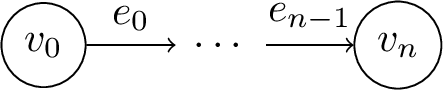 .
.
where \(v_0, \ldots, v_n\) are distinct nodes, \(e_0, \ldots, e_{n-1}\) are distinct edges (for \(n > 0\)) and each \(v_i\) has the property \(v_i.k\) defined. The node-value word of a node-annotated path is defined as \(w^N_p = v_1.k \cdot v_2.k \cdots v_n.k\).
As in Section 11, we define the node-value language of a one-way path pattern \(\psi\) as \(\mathcal{L}^N(\psi) = \{w \mid \exists (p, \mu) \in \left\llbracket\psi\right\rrbracket_p, w^N_p = w\}\).
Lemma 8. For every one-way infinitely-repeated path pattern \(\psi^{n..\infty}\) , if a word \(w \in \mathcal{L}^N(\psi^{n..\infty})\) then the word \(ww\) also belongs to \(\mathcal{L}^N(\psi^{n..\infty})\).
Proof. Let \(w\) be a word in \(\mathcal{L}^N(\psi^{n..\infty})\). By definition of \(\mathcal{L}^N\), there exists a path \(\textsf{path}(v_1, e_1, \ldots e_{k-1}, v_k)\) and a valuation \(\mu\) such that \((p, \mu) \in \left\llbracket\psi^{n..\infty}\right\rrbracket_p\) and \(w^N_p = w\). Let \(p'=\textsf{path}(v'_1, e'_1, \ldots e'_{k-1}, v'_k)\) be a copy of \(p\) with fresh ids for all elements (nodes and edges) except for \(v'_1\) for which \(id(v'_1) = id(v_k)\). By definition of path concatenation, \(p\) and \(p'\) concatenate and, since \((p, \mu) \in \left\llbracket\psi^{n..\infty}\right\rrbracket_p\), we can construct a valuation \(\mu'\) such that \((p', \mu') \in \left\llbracket\psi^{n..\infty}\right\rrbracket_{p'}\) as follows: \(\mu'(x)=v_i'\) whenever \(\mu(x)=v_i\) for all \(0 \leq i \leq k\) and \(\mu'(y)=e'_j\) whenever \(\mu(y)=e_j\) for all \(0 \leq j < k\). As \((p, \mu) \in \left\llbracket\psi^{n..\infty}\right\rrbracket_p\) (resp. \((p', \mu') \in \left\llbracket\psi^{n..\infty}\right\rrbracket_{p'}\)), it can easily be shown by induction that \((p, \mu) \in \left\llbracket\psi^{n..\infty}\right\rrbracket_{p\odot p'}\) (resp. \((p', \mu') \in \left\llbracket\psi^{n..\infty}\right\rrbracket_{p\odot p'}\)) and, by definition of the semantics of repetition, we can conclude that \((p \odot p',\mu_\emptyset) \in \left\llbracket\psi^{n..\infty}\right\rrbracket_{p\odot p'}\) and so we get that \(w^N_p \cdot w^N_{p'} = w \cdot w\) belongs to \(\mathcal{L}^N(\psi^{n..\infty})\). ◻
Lemma 9. For any one-way path patterns \(\psi, \psi', \psi''\) such that \(\mathcal{L}^N(\psi' \psi\psi'') \neq \emptyset\) and any node-value word \(w\), if \(w \in \mathcal{L}^N(\psi)\) then there exists a node-annotated path \(p\) such that \(w^N_p \in \mathcal{L}^N(\psi' \psi\psi'')\) and \(w\) is a subword of \(w^N_p\).
Proof. Let \(w\) be a word in \(\mathcal{L}^N(\psi)\). By definition of \(\mathcal{L}^N\), there exists a path \(p=\textsf{path}(v_1, e_1, \ldots, v_k)\) and an assignment \(\mu\) such that \((p, \mu) \in \left\llbracket\psi\right\rrbracket_G\) and \(w = w^N_p\) for some graph \(G\). By the semantics of concatenation and since \(\mathcal{L}^N(\psi_1 \psi\psi_2) \neq \emptyset\), there are \(p'=\textsf{path}(v'_1, e'_1, \ldots, v'_{k'})\), \(p''=\textsf{path}(v''_1, e''_1, \ldots, v''_{k''})\), \(\mu'\) and \(\mu''\) such that \((p', \mu') \in \left\llbracket\psi'\right\rrbracket_G\), \((p'', \mu'') \in \left\llbracket\psi''\right\rrbracket_G\), \(p' \odot p\), \(p \odot p''\) and \(\mu, \mu'\) and \(\mu''\) are compatible. By definition of path concatenation, \(p' \odot p \odot p'' = \textsf{path}(v'_1, e'_1, \ldots, v'_{k'}, e_1, \ldots, v_k, e''_1, \ldots v''_{k''})\) forms a path whose node-value word is \(w^N_{p' \odot p \odot p''} = v'_1.k \cdots v'_{k'}.k \cdot v_2.k \cdots v_k.k \cdot v''_2.k \cdot v''_{k''}.k\). Since the paths concatenate, we know that \(v'_{k'} = v_1\) and \(v''_1 = v_k\) and so \(w\) is a subword of \(w^N_{p' \odot p \odot p''}\). Once again by definition of concatenation, we get that \((p' \odot p \odot p'', \mu' \bowtie\mu \bowtie\mu'') \in \left\llbracket\psi' \psi\psi''\right\rrbracket_G\) and so \(w^N_{p' \odot p \odot p''} \in \mathcal{L}^N(\psi' \psi\psi'')\). ◻
The above lemma can be easily extended to concatenations of arbitrary size.
We can now prove Theorem 2.
Assume, by contradiction, that there is a one-way path pattern \(\psi\) equivalent to \(Q^{\mathsf{N}}_{\neq}\). By lemma 6, we can assume that \(\psi\) is in +NF, and so of the shape \(\psi_1+\cdots+\psi_m\), and since the language of \(Q^{\mathsf{N}}_{\neq}\) is infinite, we can further assume that at least one of the \(\psi_i\) is of the shape \(\rho_1 \ldots \rho_j^{n..\infty} \ldots \rho_k\). Let \(w\) be a word in \(\mathcal{L}^N(\rho_j^{n..\infty})\). By lemma 8, we have that \(ww\) also belongs to \(\mathcal{L}^N(\rho_j^{n..\infty})\) and, by lemma 9 we can conclude that there exists a path \(p\) and an assignment \(\mu\) such that \(ww\) is a subword of \(w^N_p\) and \((p, \mu) \in \mathcal{L}^N(\rho_1 \ldots \rho_j^{n..\infty} \ldots \rho_k)\). Since all values in \(ww\) are repeated twice, \(\psi\) cannot be equivalent to \(Q^{\mathsf{N}}_{\neq}\).
14 Proof of Theorem 4↩︎
In what follows, we focus on data-less paths which are, as before, graphs whose underlying structures are paths, without properties and labels.
Figure 11: 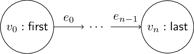 .
.
where \(n\ge 0\), and \(v_i \ne v_j\in\mathsf{N}, e_i \ne e_j\in \mathsf{E}\) for every \(i \ne j\), and \(\mathsf{lab}(v_1) = \mathsf{first},\,\mathsf{lab}(v_n)= \mathsf{last}\).
We then show that no Boolean Core GQL query returns true on \(G_n\) iff \(n\) is a power of 2.
Theorem 6. There is no Core GQL query \(\mathcal{Q}\) such that for every data-less path \(\mathbf{p}\) the following holds: \[\left\llbracket\mathcal{Q}\right\rrbracket_\mathbf{p} = \boldsymbol{true}\text{ if and only if }\, \mathsf{len}(\mathbf{p})=2^n,n\in \mathbb{N}\]
14.1 Proof of Theorem 6↩︎
For a data-less path \(\mathbf{p}_\epsilon\), we define the function \(\mathsf{pos}\) that maps each node in \(\mathbf{p}_\epsilon\) to its position (where the position of the first node in \(\mathbf{p}_\epsilon\) is \(1\)) and each edge in \(\mathbf{p}_\epsilon\) to the tagged position of its source node. We do so to distingush whether a position correspond to a node or an edge. For example, if \(\mathbf{p}_\epsilon\) is
Figure 12:  .
.
then \(\mathsf{pos}(n_j) = j\) and \(\mathsf{pos}(e_j) = j'\). We treat tagged integers as integers wrt to arithmetics and equality.
Before proving the translation from path patterns to PA, we first show that path patterns without variables can be translated to automata.
Lemma 10. For every path pattern \(\psi\) with no variables, there exists a finite automaton \(A_{\psi}\) such that \[o_1 \cdots o_{m-1} \in \mathcal{L}(A_{\psi})\, \text{iff}\, ((n_1,e_1,\ldots,n_{m-1},e_{m-1},n_m),\emptyset)\in \left\llbracket\psi\right\rrbracket_{\mathbf{p}_\epsilon}\] where \(o_j :=a\) if \(e_j\) is a forward edge (from \(n_{j-1}\) to \(n_j\)) and \(o_j :=b\) if \(e_j\) is a backward edge (from \(n_{j}\) to \(n_{j-1}\)).
Proof. We use the standard definition of finite automata. We fix the input alphabet to be \(\{a,b\}\), and prove the claim by induction on \(\psi\)’s structure.
The intuition behind the construction is that the \(a\)’s represent the forward edges and the \(b\)’s the backward edges in a path that matches \(\psi\).
As a convention, \(q_0\) and \(q_f\) denote the initial and final states, respectively.
14.1.0.1 Base cases.
\(\psi= ()\) then the automaton uses the following transitions \(\delta(q_0,\epsilon)= q_f\).
\(\psi= () \rightarrow ()\) then \(\delta(q_0,a)= q_f\).
\(\psi= () \leftarrow ()\) then \(\delta(q_0,b)= q_f\).
14.1.0.2 Induction step
For the cases \(\psi= \psi_1 + \psi_2\), \(\psi= \psi_1 \psi_2\), and \(\psi= \psi'^{*}\) we use similar construction to Thompson construction by adding epsilon transitions and redefining the initial and accepting states. It is straightforward to show that this construction satisfies the connection stated in the lemma. ◻
Corollary 3. For every path pattern \(\psi\) without variables, and every data-less path \(\mathbf{p}_\epsilon\) the set \(\{ \mathsf{pos}(n_m) -\mathsf{pos}(n_1) \mid (p,\emptyset)\in \left\llbracket\psi\right\rrbracket_{\mathbf{p}_\epsilon}, p :=(n_1, e_1,\ldots, n_{m-1},e_{m-1},n_m) \}\) is semi-linear.
Proof. The proof follows from Lemma 10, the fact that the Parikh image of a finite automaton is semilinear, and the closure of semilinear sets under subtraction. ◻
We obtain the following connection:
Lemma 11. For every data-less path \(\mathbf{p}_\epsilon\), and path pattern \(\psi\) there is a PA formula \(\varphi_{\psi}(x_s,x_1,\ldots, x_m, x_t)\) where \(\mathsf{FV}\left(\psi\right) :=\{x_1,\ldots, x_m\}\) such that \[\varphi_{\psi}(i_s,i_1,\ldots, i_m, i_t) \,\text{ if and only if }\, \exists p:\,(p,\mu) \in\left\llbracket\psi\right\rrbracket_{\mathbf{p}_\epsilon}\] where \(i_j = \mathsf{pos}(\mu(x_j))\) for every \(j\), and \(i_s,i_t\) are the positions of the first and last nodes of \(p\) in \(\mathbf{p}_\epsilon\), respectively.
Proof. We simplify \(\psi\): Since we deal with data-less paths, it is straightforward that any \(\psi_{\langle \theta \rangle}\) can be rewritten to \(\psi\) while preserving the semantics (on data-less paths). Formally, for every data-less path \(P\) and for every condition \(\theta\), it holds that \(\left\llbracket\psi\right\rrbracket_P = \left\llbracket\psi_{\langle \theta \rangle}\right\rrbracket_P\). In addition, we can assume that every repetition \(\psi^{n..m}\) where \(m<\infty\) can be rewritten to \(\cup_{i=n}^m \psi_i\). This is true for any input (no need to restrict to data-less paths) due to the semantics definition. For repetition \(\psi^{n..m}\) with \(m=\infty\), we can rewrite the pattern and obtain \(\psi^{n} \psi^{0..\infty}\). Also here, equivalence holds for any input (no need to restrict to data-less paths) due to the semantics definition. Recall that now we focus only on path patterns in which we disallow having variables on the edges.
Under the above assumptions on the form of \(\psi\), we define \(\varphi_{\psi}\) inductively as follows:
If \(\psi:=(x)\) then \(\varphi_{\psi}(x_s,x,x_{t}) :=x_s= x \wedge x=x_{t}\);
If \(\psi:=()\) then \(\varphi_{\psi}(x_s,x_{t}) :=x_s=x_{t}\);
If \(\psi:=(x)\rightarrow(y)\) then \(\varphi_{\psi}(x_s,x,y,x_t) :=y=x+1 \wedge x=x_s \wedge y=y_s\)
If \(\psi:=(x)\leftarrow(y)\) then \(\varphi_{\psi}(x_s,x,y,x_t) :=x=y+1 \wedge x=x_s \wedge y=y_s\)
If \(\psi:=\overset{x}{\rightarrow}\) then \(\varphi_{\psi}(x_s,x,x_t) :=x_t = x_s+1 \wedge x=x_s\)
If \(\psi:=\psi_1 \psi_2\) then \(\varphi_{\psi}(x_s,\bar{z}, y_t) :=\varphi_{\psi_1}(x_{s},\bar{x},x_t) \wedge \varphi_{\psi_2}(y_s,\bar{y},y_t) \wedge x_t = y_s\) where \(\bar{z}\) is the union \(\bar{x}\cup \bar{y}\).
If \(\psi:=\psi_1 + \psi_2\) then \(\varphi_{\psi}(x_s,\bar{x}, x_t) :=\varphi_{\psi_1}(x_s,\bar{x}, x_t) \vee \varphi_{\psi_2}(x_s,\bar{x}, x_t)\).
If \(\psi:=\psi_1^{n}\) then \(\varphi_{\psi}(x_s,x_t) = \exists x_1,y_1,\bar{z}_1\ldots,x_n, y_{n}, \bar{z}_n:\; \bigwedge_{i=1}^n\varphi_{\psi_1}(x_i,\bar{z}_i,y_i) \wedge \bigwedge_{i=1}^{n-1} y_{i}=x_{i+1} \wedge x_1 = x_s \wedge y_n = x_t\)
If \(\psi:=\psi_1^{*}\) then, due to Corollary 3, there is a PA formula \(\psi_{\psi_1^{*}}(m)\) for \(\{ |p| \mid (p,\emptyset) \in \left\llbracket\psi_1^{*}\right\rrbracket_{\pm} \}\). Therefore, \(\varphi_{\psi}(x_s,x_t) :=\exists m: x_t = x_s+ \psi_{\psi_1^{*}}(m)\)
Showing that the condition in the Lemma holds for \(\varphi_{\psi}\) is straightforward from the definition. ◻
Lemma 12. For every data-less path \(\mathbf{p}_\epsilon\), and path pattern with output \(\psi_{\Omega}\) with variables only on nodes, there is a PA formula \(\varphi_{\psi}(x_1,\ldots, x_m)\) where \(\Omega:=\{x_1,\ldots, x_m\}\) such that \[\varphi_{\psi_{\Omega}}(i_1,\ldots, i_m) \,\text{ if and only if }\, \mu \in\left\llbracket\psi\right\rrbracket_{\mathbf{p}_\epsilon}\] where \(i_j = \mathsf{pos}(\mu(x_j))\) for every \(j\).
Proof. Notice that since we are dealing with dataless paths as input, all elements in \(\Omega\) are variables. Hence, the proof is implied directly from Lemma 11. In particular, by existentially quantifying over variables that are omitted in \(\Omega\). For example,\[\begin{align} &\text{if}\, \varphi_{\psi}(x_s,\bar{x}, \bar{y} , x_t) \,\text{then}\,\varphi_{\psi_{ \bar y}}(\bar{y} ) = \exists x_s,\bar x,x_t:\, \varphi_{\psi}(x_s,\bar{x}, \bar{y} , x_t) \\ &\text{if}\, \varphi_{\psi}(x_s,\bar{x}, \bar{z},\bar{y} , x_t) \,\text{then}\,\varphi_{\psi_{ \bar{y}\bar{x}}}( \bar{y},\bar{x} ) = \exists x_s,\bar{z},x_t:\, \varphi_{\psi}(x_s,\bar{x}, \bar{z},\bar{y} , x_t) \end{align}\] ◻
Lemma 13. For every data-less path \(\mathbf{p}_\epsilon\), and Core GQL query \(\mathcal{Q}\), there is a PA formula \(\varphi_{\mathcal{Q}}(x_1,\ldots, x_m)\) such that \(\mathsf{attr}(\mathcal{Q}) = \{x_1,\ldots, x_m\}\) and \[\varphi_{\mathcal{Q}}(i_1,\ldots, i_m) \,\text{ if and only if }\, \mu \in\left\llbracket\mathcal{Q}\right\rrbracket_{\mathbf{p}_\epsilon}\] where \(i_j = \mathsf{pos}(\mu(x_j))\) for every \(j\).
Proof. The proof is by induction on the structure of \(\mathcal{Q}\). The base case of path pattern with output is covered by the previous lemma. For the induction step, we distinguish between the form of \(\mathcal{Q}\).
If \(\mathcal{Q}:=\psi_{\mathbf{A}}(\mathcal{Q}')\) then \(\varphi_{\mathcal{Q}}(\bar z) :=\exists \bar y \, \varphi_{\mathcal{Q}'}(x_1,\ldots, x_m)\) where \(\bar y = \mathbf{A} \setminus \{x_1,\ldots, x_m\}\) and \(\bar z = \mathbf{A} \cap \{x_1,\ldots, x_m\}\).
If \(\mathcal{Q}:=\sigma_{\theta}(\mathcal{Q}')\) then \(\varphi_{\mathcal{Q}}(\bar x) :=\varphi_{\mathcal{Q}'}(\bar x)\). Notice that the correctness here follows from the fact the input is a data-less path.
If \(\mathcal{Q}:=\rho_{A\rightarrow A'}(\mathcal{Q}')\) then \(\varphi_{\mathcal{Q}}(\bar{x}, A, \bar{y} ) := \varphi_{\mathcal{Q}'}(\bar{x}, A', \bar{y} )\).
If \(\mathcal{Q}:=\mathcal{Q}_1 \times \mathcal{Q}_2\) then \(\varphi_{\mathcal{Q}}(\bar{x}) :=\varphi_{\mathcal{Q}_1}(\bar{z}) \wedge \varphi_{\mathcal{Q}_2}(\bar{y})\) with \(\bar{x}\) the union of \(\bar{z}\) and \(\bar{y}\).
If \(\mathcal{Q}:=\mathcal{Q}_1 \cup \mathcal{Q}_2\) then \(\varphi_{\mathcal{Q}}(\bar{x}) :=\varphi_{\mathcal{Q}_1}(\bar{x}) \vee \varphi_{\mathcal{Q}_2}(\bar{x})\).
If \(\mathcal{Q}:=\mathcal{Q}_1 \cap \mathcal{Q}_2\) then \(\varphi_{\mathcal{Q}}(\bar{x}) :=\varphi_{\mathcal{Q}_1}(\bar{x}) \wedge \varphi_{\mathcal{Q}_2}(\bar{x})\).
If \(\mathcal{Q}:=\mathcal{Q}_1 \setminus \mathcal{Q}_2\) then \(\varphi_{\mathcal{Q}}(\bar{x}) :=\varphi_{\mathcal{Q}_1}(\bar{x}) \wedge \neg \varphi_{\mathcal{Q}_2}(\bar{x})\).
Showing that the condition holds is straightforward from the definition. ◻
Proof of Theorem 6. Let us assume by contradiction that there is a Boolean GQL query \(\mathcal{Q}\) for which \(\left\llbracket\mathcal{Q}\right\rrbracket_{\mathbf{p}_\epsilon} \ne \emptyset\) if and only if \(\mathsf{len}(\mathbf{p}_\epsilon)=2^n\), \(n\in \mathbb{N}\).
Let us define a new query \(\mathcal{Q}'\) that binds \(x\) to the last node of a data-less path. We set \(\mathcal{Q}' :=\psi_1 \setminus \psi_2\) where \(\psi_1 :=()\rightarrow^{*}(x)\) and \(\psi_2 :=()\rightarrow^{*}(x)\rightarrow ()\). It holds that \(\left\llbracket\mathcal{Q}'\right\rrbracket_{\mathbf{p}_\epsilon} :=\{\mu \mid \mathsf{dom}(\mu)= \{x\}, \mu(x) = n_k \}\) where \(n_k\) is the last node in \(\mathbf{p}_\epsilon\). Now let us consider \(\mathcal{Q}\times \mathcal{Q}'\). It can be easily shown that \(\left\llbracket\psi_x(\mathcal{Q}\times \mathcal{Q}')\right\rrbracket_{\mathbf{p}_\epsilon} \ne \emptyset\) iff \(\left\llbracket\mathcal{Q}\right\rrbracket_{\mathbf{p}_\epsilon} \ne \emptyset\). By previous lemma, \(\left\llbracket\psi_x(\mathcal{Q}\times \mathcal{Q}')\right\rrbracket_{\mathbf{p}_\epsilon}\) is expressible by a PA formula. Nevertheless, by our assumption \(\left\llbracket\psi_x(\mathcal{Q}\times \mathcal{Q}')\right\rrbracket_{\mathbf{p}_\epsilon}\) is exactly the set \(\{2^n \mid n\in \mathbb{N} \}\) which leads to the desired contradiction. ◻
14.2 Datalog on Graphs↩︎
Datalog↩︎
Let \(\mathcal{S}\) be a schema. An atom over \(\mathcal{S}\) is an element of the form \(S(x_1,\ldots, x_k)\) where \(S\in\mathcal{S}\), \(\mathsf{arity}(S)=k\) and \(x_1,\ldots x_k\) is a sequence of variables with no repetitions. A Datalog program is a tuple \((\mathcal{E},\mathcal{I},\Phi,\mathtt{Out})\) where \(\mathcal{E}\) and \(\mathcal{I}\), namely the IDB and EDB signatures, respectively, are disjoint schemas, \(\mathtt{Out}\) is a designated relation symbol in \(\mathcal{I}\), and \(\Phi\) is a set of rules \(\rho\) of the form \[\varphi\leftarrow \varphi_1 , \ldots, \varphi_m\] where \(\varphi\) is an atom over \(\mathcal{I}\), and each \(\varphi_i\) is an atom over \(\mathcal{I}\cup \mathcal{E}\). We restrict further the rules by allowing only cases in which each variable in the head \(\varphi\) of \(\rho\) occurs also in its body, namely \(\varphi_1, \ldots, \varphi_m\).
The semantics \(\left\llbracket P\right\rrbracket_{\mathcal{D}}\) of a Datalog program \(P :=(\mathcal{E},\mathcal{I},\Phi,\mathtt{Out})\) over a database \(\mathcal{D}\) is defined in the standard way as we recall now: Given a database \(\mathcal{D}\) over a schema \(\mathbf{S}\), a partial mapping \(\mu:\mathsf{Vars}\rightarrow \mathbf{U}\) satisfies an atom \(\varphi(x_1,\ldots,x_k)\) (w.r.t. \(\mathcal{D}\)) if \(\varphi\in \mathbf{S}\) and \((\mu(x_1),\ldots,\mu(x_k))\in \mathcal{D}({\varphi})\). A database \(\mathcal{D}'\) satisfies a rule \(\rho\) if every partial mapping \(\mu\) that satisfies each of \(\rho\)’s body atoms w.r.t. \(\mathcal{D}'\), also satisfies its head atom. A database \(\mathcal{D}'\) satisfies a set \(\Phi\) of rules if it satisfies every \(\rho\in \Phi\). We define the semantics \(\left\llbracket P\right\rrbracket_{\mathcal{D}} :=\mathcal{D}'\) such that (1) \(\mathcal{D}'\) satisfies \(\Phi\) and (2) every \(\mathcal{D}''\) that satisfies \(\Phi\) has the following property: every relation symbol \(R \in \mathcal{I}\cup \mathcal{E}\), the set \(\mathcal{D}'(R) \subseteq \mathcal{D}''(R)\). We say that \(P\) is Boolean if \(\mathsf{arity}(\mathtt{Out}) = 0\), and in this case, we say it outputs \(\boldsymbol{true}\) if \(\mathtt{Out}() \in\left\llbracket P\right\rrbracket_{\mathcal{D}}\).
Datalog over property graphs
We view property graphs \(G :=\langle N, E, \mathsf{lab}, \mathsf{src}, \mathsf{tgt}, \mathsf{prop}\rangle\) as relational structures \(\mathcal{D}_G\) over the relational schema consisting of relation symbols \(N, E, \mathsf{lab}, \mathsf{src}, \mathsf{tgt}, \mathsf{prop}\) with the straightforward interpretation.
Example 1. The Datalog program defined by the rules: \[\begin{align} \mathsf{eqLen}(x,y,z,w) &\leftarrow E(x,y),E(z,w)\\ \mathsf{eqLen}(x,y,z,w) &\leftarrow \mathsf{eqLen}(x,y',z,w'), E(y',y),E(w'w) \end{align}\] extracts from a bounded data-less path bindings \(\mu\) of \(x,y,z,w\) such that the number of edges between \(\mu(x)\) and \(\mu(y)\) equals to that between \(\mu(z)\) and \(\mu(w)\).
Example 2. The Datalog program given by the rules \[\begin{align} \mathsf{len}_{2^n}(x,y) &\leftarrow E(x,z),E(z,y) \\ \mathsf{len}_{2^n}(x,y) &\leftarrow \mathsf{len}_{2^n}(x,z), \mathsf{len}_{2^n}(w,y), \mathsf{eqLen}(x,z,w,y) \\ \mathtt{Out}() &\leftarrow \mathsf{len}_{2^n}(x,y), \mathsf{lab}(x,\mathsf{first}), \mathsf{lab}(y,\mathsf{last}) \end{align}\] outputs \(\boldsymbol{true}\) if and only if the length of the input bounded data-less path is \(2^n\) for some \(n\in \mathbb{N}\).
Using a straightforward induction, we can show that:
Lemma 14. For every Datalog program \(P\) and data-less paths \(p,p\)’, if \(p\sim p'\) then \(\left\llbracket P\right\rrbracket_{\mathcal{D}_{p'}} = \left\llbracket P\right\rrbracket_{\mathcal{D}_p}\).
We denote \(\mathcal{D}_p\) by the \(\mathcal{D}_n\) where \(n\) is the length of \(p\). We can view Boolean Datalog Programs as queries on the quotient space \(P/\sim\) and define \[\mathsf{len}(P) :=\{n \mid \left\llbracket P\right\rrbracket_{\mathcal{D}_{n}} = \boldsymbol{true}\}.\] We can conclude:
Corollary 4. Datalog over property graphs is strictly more expressive than GQL. There is a Datalog over property graphs program such that for every data-less path \(\mathbf{p}\) the following holds: \[\left\llbracket\mathcal{Q}\right\rrbracket_\mathbf{p} = \boldsymbol{true}\text{ if and only if }\, \mathsf{len}(\mathbf{p})=2^n,n\in \mathbb{N}\]
14.3 Proof of Theorem 4↩︎
The proof follows directly from Theorem 6 and Corollary [cor:dl2pown].
References↩︎
[1]
H. Gaifman and M. Y. Vardi, “A simple proof that connectivity of finite graphs is not first-order definable,” Bull. EATCS, vol. 26, pp. 43–44,
1985.
[2]
R. Fagin, “Monadic generalized spectra,” Math. Log. Q., vol. 21, no. 1, pp. 89–96, 1975, doi: 10.1002/MALQ.19750210112.
[3]
A. V. Aho and J. D. Ullman, “The universality of data retrieval languages,” in Conference record of the sixth annual ACM symposium on principles of
programming languages, san antonio, texas, USA, january 1979, 1979, pp. 110–120, doi: 10.1145/567752.567763.
[4]
A. Eisenberg and J. Melton, “SQL: 1999, formerly known as SQL 3,” SIGMOD Rec., vol. 28, no. 1, pp. 131–138, 1999, doi: 10.1145/309844.310075.
[5]
I. F. Cruz, A. O. Mendelzon, and P. T. Wood, “A graphical query language supporting recursion,” in Proceedings of the association for computing machinery special interest
group on management of data 1987 annual conference, san francisco, CA, USA, may 27-29, 1987, 1987, pp. 323–330, doi: 10.1145/38713.38749.
[6]
D. Calvanese, G. D. Giacomo, M. Lenzerini, and M. Y. Vardi, “Containment of conjunctive regular path queries with inverse,” in KR 2000, principles of
knowledge representation and reasoning proceedings of the seventh international conference, breckenridge, colorado, USA, april 11-15, 2000, 2000, pp. 176–185.
[7]
P. Barceló, L. Libkin, A. W. Lin, and P. T. Wood, “Expressive languages for path queries over graph-structured data,” ACM Trans. Database Syst., vol.
37, no. 4, pp. 31:1–31:46, 2012.
[8]
P. Barceló, “Querying graph databases,” in Principles of database systems (PODS), 2013, pp. 175–188.
[9]
R. Angles, M. Arenas, P. Barceló, A. Hogan, J. L. Reutter, and D. Vrgoc, “Foundations of modern query languages for graph databases,” ACM Comput. Surv.,
vol. 50, no. 5, pp. 68:1–68:40, 2017.
[10]
L. Libkin, W. Martens, and D. Vrgoč, “Querying graphs with data,” Journal of the ACM, vol. 63, no. 2, pp. 14:1–14:53, 2016.
[11]
M. Benedikt, A. W. Lin, and D.-D. Yen, “Revisiting the expressiveness landscape of data graph queries,” CoRR, vol. abs/2406.17871, 2024, doi: 10.48550/ARXIV.2406.17871.
[12]
W. Martens, M. Niewerth, and T. Popp, “A trichotomy for regular trail queries,” Log. Methods Comput. Sci., vol. 19, no. 4, 2023, doi: 10.46298/LMCS-19(4:20)2023.
[13]
J. L. Reutter, M. Romero, and M. Y. Vardi, “Regular queries on graph databases,” Theory Comput. Syst., vol. 61, no. 1, pp. 31–83, 2017, doi: 10.1007/s00224-016-9676-2.
[14]
M. F. Fernandez, D. Florescu, A. Y. Levy, and D. Suciu, “A query language for a web-site management system,” SIGMOD Rec., vol. 26, no. 3, pp. 4–11,
1997, doi: 10.1145/262762.262763.
[15]
P. Selmer, https://www.gqlstandards.org/existing-languages“Existing languages working group: GQL influence graph.” 2019.
[16]
T. Lindaaker, “Predicates on sequences of edges,” ISO/IEC JTC1/ SC32 WG3:W26-027, 2023.
[17]
F. Zemke, “For each segment discussion,” ISO/IEC JTC1/ SC32 WG3:BGI-022, 2024.
[18]
N. Francis et al., “A researcher’s digest of GQL,” in 26th international conference on database theory, ICDT 2023, march 28-31, 2023,
ioannina, greece, 2023, vol. 255, pp. 1:1–1:22, doi: 10.4230/LIPICS.ICDT.2023.1.
[19]
N. Francis et al., “GPC: A pattern calculus for property graphs,” in Proceedings of the 42nd ACM
SIGMOD-SIGACT-SIGAI symposium on principles of database systems, PODS 2023, seattle, WA, USA, june 18-23, 2023, 2023, pp. 241–250, doi: 10.1145/3584372.3588662.
[20]
L. Libkin, Elements of finite model theory. Springer, 2004.
[21]
O. van Rest, S. Hong, J. Kim, X. Meng, and H. Chafi, “PGQL: A property graph query language,” in Proceedings of the fourth international workshop on graph
data management experiences and systems, 2016, pp. 1–6.
[22]
B. R. Bebee et al., “Amazon Neptune: Graph data management in the cloud,” in Proceedings of the ISWC 2018 posters &
demonstrations, industry and blue sky ideas tracks co-located with 17th international semantic web conference (ISWC 2018), monterey, USA, october 8th - to - 12th, 2018, 2018, vol. 2180, [Online]. Available: https://ceur-ws.org/Vol-2180/paper-79.pdf.
[23]
A. Deutsch, Y. Xu, M. Wu, and V. E. Lee, “Aggregation support for modern graph analytics in TigerGraph,” in Proceedings of the 2020 international conference on
management of data, SIGMOD conference 2020, 2020, pp. 377–392, doi: 10.1145/3318464.3386144.
[24]
S. Abriola, P. Barceló, D. Figueira, and S. Figueira, “Bisimulations on data graphs,” J. Artif. Intell. Res., vol. 61, pp. 171–213, 2018, doi: 10.1613/JAIR.5637.
[25]
C. Sharma, R. Sinha, and K. Johnson, “Practical and comprehensive formalisms for modelling contemporary graph query languages,” Inf. Syst., vol. 102, p. 101816,
2021, doi: 10.1016/J.IS.2021.101816.
[26]
A. Deutsch et al., “Graph pattern matching in GQL and SQL/PGQ,” in SIGMOD, 2022, pp. 1–12, [Online]. Available: https://arxiv.org/abs/2112.06217.
[27]
D. ten Wolde, G. Szárnyas, and P. A. Boncz, “DuckPGQ: Bringing SQL/PGQ to DuckDB,” Proc. VLDB Endow., vol. 16, no. 12, pp. 4034–4037,
2023, doi: 10.14778/3611540.3611614.
[28]
PRQL, https://prql-lang.orgPipelined relational query language. 2024.
[29]
J. Shute et al., “SQL has problems. We can fix them: Pipe syntax in SQL,” Proc. VLDB Endow., vol. 17, no. 12, pp.
4051–4063, 2024, [Online]. Available: https://www.vldb.org/pvldb/vol17/p4051-shute.pdf.
[30]
H. Wickham, R. François, L. Henry, K. Müller, and D. Vaughan, R package version 1.1.4, https://github.com/tidyverse/dplyrDplyr: A grammar of
data manipulation. 2023.
[31]
P. Hell and J. Nešetřil, Graphs and homomorphisms. Oxford University Press, 2004.
[32]
N. Yakovets, P. Godfrey, and J. Gryz, “Evaluation of SPARQL property paths via recursive SQL,” in Proceedings of the 7th alberto mendelzon
international workshop on foundations of data management, puebla/cholula, mexico, may 21-23, 2013, 2013, vol. 1087, [Online]. Available: https://ceur-ws.org/Vol-1087/paper11.pdf.
[33]
W. Sun, A. Fokoue, K. Srinivas, A. Kementsietsidis, G. Hu, and G. T. Xie, “SQLGraph: An efficient relational-based property graph store,” in Proceedings of the 2015
ACM SIGMOD international conference on management of data, melbourne, victoria, australia, may 31 - june 4, 2015, 2015, pp. 1887–1901, doi: 10.1145/2723372.2723732.
[34]
S. Abiteboul and V. Vianu, “Computing with first-order logic,” J. Comput. Syst. Sci., vol. 50, no. 2, pp. 309–335, 1995, doi: 10.1006/JCSS.1995.1025.
[35]
M. Arenas, P. Barceló, L. Libkin, W. Martens, and A. Pieris, Database theory. Open source at https://github.com/pdm-book/community, 2022.
[36]
S. Ginsburg and E. H. Spanier, “Bounded Algol-like languages,” Transactions of the American Mathematical Society, vol. 113, pp. 333–368, 1964.
[37]
F. N. Afrati, M. Gergatsoulis, and F. Toni, “Linearisability on datalog programs,” Theor. Comput. Sci., vol. 308, no. 1–3, pp. 199–226, 2003, doi: 10.1016/S0304-3975(02)00730-2.
[38]
N. Immerman, Descriptive complexity. Springer, 1999.
[39]
B. Bollobás, Random graphs, vol. 73. Cambridge University Press, 2011.
[40]
A. E. Hodler and M. Needham, “Graph data science using Neo4j,” in Massive graph analytics, D. A. Bader, Ed.
Chapman; Hall/CRC, 2022, pp. 433–457.
[41]
S. Han and Z. G. Ives, “Implementation strategies for views over property graphs,” Proc. ACM Manag. Data, vol. 2, no. 3, p. 146, 2024, doi: 10.1145/3654949.
This work is licensed under the Creative Commons BY-NC-ND 4.0 International License. Visit https://creativecommons.org/licenses/by-nc-nd/4.0/ to view a copy of this license. For any use beyond those covered by this license, obtain permission by emailing info@vldb.org. Copyright is held by the owner/author(s). Publication rights licensed to the VLDB Endowment.
Proceedings of the VLDB Endowment, Vol. 18, No. 6ISSN 2150-8097.
doi:10.14778/3725688.3725707
↩︎The testing program is written in Go and communicates with Neo4j (v5.18.1) via the Neo4j Go driver. All tests were executed on a machine with the following configuration: 16 Intel i7-10700 @ 2.90GHz CPUs, 16GB RAM, Ubuntu 22.04.3 LTS↩︎
Notice that it can be the case that \(\mathcal{L}(\psi_i) = \mathcal{L}(\rho_1) \mathcal{L}( \rho)^{n..\infty} \mathcal{L}(\rho_2) \langle \theta \rangle\) in which case the sequel of the proof still holds since the condition \(\theta\) can only refer to variables in \(\rho_1,\rho_2\).↩︎
Liat: Can elaborate more depending on which part of \(w\) the pumped part conforms to.…↩︎