Uniform K-stability of \(G\)-varieties of complexity 1
January 01, 1970
Abstract
Let \({\rm k}\) be an algebraically closed field of characteristic 0 and \(G\) a connected, reductive, linear algebraic group of simply connected type over \({\rm k}\). Let \(X\) be a projective \(G\)-variety of complexity 1. We classify \(G\)-equivariant normal test configurations of \(X\) with integral central fibre via the combinatorial data. We also give a formula of anti-canonical divisors on \(X\). Based on this formula, when \(X\) is \(\mathbb{Q}\)-Fano, we give an expression of the Futaki invariant, and derive a criterion of uniform K-stability in terms of the combinatorial data.
1 Introduction↩︎
The famous Yau-Tian-Donaldson conjecture asserts that the existence of Kähler-Einstein metrics on a Fano manifold is equivalent to the K-stability. The conjecture has been proved by Tian [1] and Chen-Donaldson-Sun [2] alternatively. In recent years, the conjecture has been widely extended to other canonical metrics (such as solitons, cscK metrics on polarized vareities), log pairs, and a uniform version for singular \(\mathbb{Q}\)-Fano varieties, see [3]–[5], etc.
The notion of K-stability was first introduced by Tian [6] in terms of special degenerations and then reformulated by Donaldson [7] in an algebro-geometric way via test-configurations. In general, to test K-stability one has to study infinitely many possible degenerations. A natural question is how to reduce it to a finitely dimensional process. The reduction would be possible when considering varieties with large group actions and the respective equivariant K-stability.
Let \({\rm k}\) be an algebraically closed field of characteristic 0 and \(G\) a connected, reductive, linear algebraic group over \({\rm k}\). Let \(X\) be a normal variety with a regular \(G\)-action. Fix any Borel subgroup \(B\) of \(G\). The complexity of the \(G\)-action on \(X\) is the codimension of a \(B\)-orbit in general position (cf. [8]). The varieties of complexity 0 are called spherical varieties, which include the well-known toric varieties. The geometry of spherical varieties has been comprehensively studied by various of authors, we refer to [9]–[12], and references therein for more knowledge. The spherical variety has a nice combinatorial description which brings great convenience to the study of its geometric structure. Roughly speaking, given a spherical variety \(X\), one may begin with the lattice \(\Gamma\) of \(B\)-semiinvariant rational functions3, which is contained in the lattice \(\mathfrak X(B)\) of \(B\)-weights, and its (\(\mathbb{Q}\)-)dual \(\Gamma_\mathbb{Q}^*\) in which the set of \(G\)-valuations (called its valuation cone, which is a solid cosimplicial cone) is embedded. The variety \(X\) itself is fully characterised by a fan of convex cones (more precisely, coloured cones, see [9], [11], [12] for details), while line bundles are described by piecewise linear functions on this fan (cf. [13], [14]). In particular, when \(X\) is polarized by some ample line bundle \(L\), there is a nice moment polytope in \(\Gamma_\mathbb{R}:=\Gamma\otimes_\mathbb{Q}\mathbb{R}\) that encodes the structure of \(G\)-modules on the spaces of sections \({\rm H}^0(X,L^k)\) for \(k\in\mathbb{N}\). In terms of these data, in recent years several combinatorial criterions of K-stability of spherical varieties were established, which give a practical way to test K-stability and provide rich examples. For instance, the K-stability criterion for toric varieties was studied by Donaldson [7], for spherical varieties established by Delcroix [15], [16], etc. It turns out that in these cases K-stability is characterised by certain barycenter of the moment polytope.
It is then natural to consider \(G\)-varieties of complexity 1. In fact, many examples in the literatures belong to this class, see for instance [17], [18]. The classification theory of \(G\)-varieties of complexity 1 was established by Timashëv [19]. In particular [19] gives a combinatorial description of these varieties analogous to the spherical cases. Unlike the spherical case, a \(B\)-semiinvariant rational function can not be completely determined only by its weight. In this case we need to consider the hyperspace instead of \(\Gamma_\mathbb{Q}^*\) in which the \(G\)-valuations are embedded. Roughly speaking, the hyperspace is a family of half-spaces \(\{\mathscr Q_{x,+}|x\in C\}\) parameterized by points of a smooth projective curve \(C\), each isomorphic to \(\Gamma_\mathbb{Q}^*\times \mathbb{Q}_+\), that glued together along common boundary \(\mathscr Q=\Gamma_\mathbb{Q}^*\times\{0\}\). The valuation cone is obtained by gluing a collection of solid convex cones in \(\mathscr Q_{x,+}\) along common face in \(\mathscr Q\). Varieties with given field of rational functions are classified by fans of coloured cones and hypercones (a hypercone is again a family of cones that glued along common boundary). The combinatorial theory of line bundles on \(G\)-varieties of complexity 1 was then studied in [14]. Line bundles are described by collection of linear functionals defined on \(\mathscr Q_{x,+}\) with common restriction on \(\mathscr Q\). See Section 2.2 for details. For \(T\)-varieties of complexity 1 with \(T\) an algebraic torus, Ilten-Süß [20] developed the classification theory of polarized \(T\)-varieties of complexity 1. They introduced the “divisorial polytope" which turns out to be a very useful tool in the study of polarized \(T\)-varieties of complexity 1. Based on this theory, they obtained a combinatorial criterion of equivariantly K-(poly)stability of Fano \(T\)-varieties of complexity 1 in [21]. Recently Rogers [22] studied K-(poly)stability of smooth Fano \({\rm SL_2}\)-varieties of complexity 1.
Let \(G\) be an arbitrary connected, reductive, linear algebraic group of simply connected type, and \(X\) a projective \(G\)-variety of complexity 1. Motivated by the works cited above, in this paper we give a criterion of \(G\)-equivariantly uniform K-stability in terms of its combinatorial data. To this end, we will first classify \(G\)-equivariant normal test configuration of \(X\) with integral central fibre. This class in particular includes the special test configurations, which are enough for testing K-stability of a \(\mathbb{Q}\)-Fano variety (cf. [4], [23]). We call \(X\) a \(\mathbb{Q}\)-Fano variety if \(X\) is \(\mathbb{Q}\)-Gorenstein and \(K_X^{-1}\) is ample. When \(X\) is \(\mathbb{Q}\)-Fano, we then consider a family of polytopes \(\{\Delta_x^O(K_X^{-1})\subset\mathfrak X_\mathbb{R}(B)\times\mathbb{R}|x\in C\}\) that encodes the information of K-stability of \(X\), where \(C\cong\mathbb{P}^1\) is birational to the rational quotient for the \(B\)-action. These polytopes were first introduced in [21] to characterize K-stability of \(T\)-varieties of complexity 1. Based on a formula of \(B\)-stable anti-canonical divisors of \(X\) derived in Section 3, it turns out that the Futaki invariant can be expressed in a very simple way on this family of polytopes. Finally we prove a combinatorial criterion of K-stability if \(X\) in addition has at most klt singularities. Let \(\mathscr V\) be the valuation cone of \(X\) and \(\mathscr V_x\) its intersection with the hyperspace over \(x\in C\), \(\mathscr A_x\subset\mathscr V_x\) the space parameterizing one-parameter subgroups in the \(G\)-equivariant automorphism group \({\rm Aut}_G(X)\) of \(X\) (see Section 4.2.1 below). Denote by \(\kappa_P\) the sum of unipotent roots of the associated parabolic subgroup \(P\) of \(X\) (see Section 2.3.2 below). Then each \(\Delta_{x}^O(K_X^{-1})\) is in fact a solid convex polytope in \((\Gamma_\mathbb{R}+\kappa_P)\times\mathbb{R}\). Also set \[{\mathbf{b}}(\Delta_{x}^O(K_X^{-1})):=\frac{1}{V}\int_{\Delta_{x}^O(K_X^{-1})}(\lambda,t)\pi(\lambda)d\lambda\wedge dt\] the barycenter of a polytope \(\Delta_{x}^O(K_X^{-1})(\subset(\Gamma_\mathbb{R}+\kappa_P)\times\mathbb{R})\), where \((\lambda,t)\) are coordinates on \(\Delta_{x}^O(K_X^{-1})\), \(\pi(\lambda)\) is a non-negative polynomial function depends on \(X\), \(d\lambda\) the standard Lebesgue measure on \(\Gamma_\mathbb{R}+\kappa_P\) which is normalized by the lattice \(\Gamma\), and \[V=\int_{\Delta_{x}^O(K_X^{-1})}\pi(\lambda)d\lambda\wedge dt\] is the volume of \(\Delta_{x}^O(K_X^{-1})\) which is in fact independent of \(x\) (see Section 5.2 below for details). We have the following
Theorem 1. Let \(X\) be a projective, \(\mathbb{Q}\)-Fano \(G\)-varieties of complexity 1 with klt singularities, which satisfies \({\rm k}(X)^B\cong{\rm k}(\mathbb{P}^1)\). Then \(X\) is \(G\)-equivariantly K-semistable if and only if \[\begin{align} \label{K-ss-eq} \kappa_P-\mathbf{b}(\Delta_{x}^O(K_X^{-1}))\in(\mathscr V_x)^\vee,~\forall x\in C, \end{align}\qquad{(1)}\] where \((\mathscr V_x)^\vee\) is the dual cone of \(\mathscr V_x\). Moreover, the following conditions are equivalent:
It holds ?? and \[\begin{align} \label{K-ps-eq} (\kappa_P-\mathbf{b}(\Delta_{x}^O(K_X^{-1})))^\perp\cap \mathscr V_x=\mathscr A_x,~\forall x\in C; \end{align}\qquad{(2)}\]
\(X\) is \(G\)-equivariantly K-polystable;
\(X\) is \({\mathbf{G}}\)-uniformly K-stable, provided \(X\) is not a \(G\times{\rm k}^\times\)-spherical variety. Here \({\mathbf{G}}\) is the subgroup of the automorphism group \({\rm Aut}(X)\) generated by \(G\) and a torus \({\mathbf{T}}\) contained in the central automorphism group of \(X\) whose Lie algebra is the linear part of \(\mathscr V\) (see Section 2.2.3 below).
Precise definitions and useful properties of the terms involved here can be found in the preliminary section and indicated above places. By the famous Yau-Tian-Donaldson conjecture [1], [4], when \({\rm k}=\mathbb{C}\) the above K-stability criterion then provides an existence criterion of Kähler-Einstein metrics.
Remark 2. Note that when \(X\) is a \(\mathbb{Q}\)-Fano \(G\times{\rm k}^\times\)-spherical variety, the K-stability can be tested by the combinatorial criterion of Delcroix [15].
As mentioned above, we need to derive a formula of \(B\)-stable anti-canonical divisors which helps to simplify the Futaki invariant. The following is a counterpart of a result of Brion [24] for spherical varieties.
Theorem 3. Let \(X\) be a \(\mathbb{Q}\)-Gorenstein, projective \(G\)-variety of complexity 1, and \(\mathscr B(X)\) the set of its \(B\)-stable prime divisors. Denote by \(P\subset G\) its associated parabolic subgroup. Then there is a \(B\)-stable anti-canonical \(\mathbb{Q}\)-divisor of \(X\), \[\begin{align} \label{anti-can-div-in-all} \mathfrak d=\sum_{D\in\mathscr B(X), h_D\not=0}(1-h_D+h_Da_{x_D})D+\sum_{D\in\mathscr B(X)^G, h_D=0}D+\sum_{D\in\mathscr D^B, h_D=0}\bar m_DD, \end{align}\qquad{(3)}\] where \(v_D=h_Dq_{x_D}+\ell_D\in\mathscr Q_{x_D,+}\) is the valuation defined by \(D\), \(\mathfrak a:=\sum_{x\in\mathbb{P}^1}a_x[x]\) is an anti-canonical \(\mathbb{Q}\)-divisor of \(C\). The coefficient \(\bar m_D\) of each colour \(D\) with \(h_D=0\) is explicitly defined in ?? and 21 . Moreover, if \(m\mathfrak d\) is a Cartier divisor for some \(m\in\mathbb{N}_+\), then \(m\mathfrak d\) is the divisor of a \(B\)-semiinvariant rational section of \(K_X^{-m}\) with weight \(m\kappa_P\).
As will be seen below, there are two classes of \(G\)-varieties of complexity one, the one-parameter and quasihomogeneous ones. For this reason Theorem 3 will be proved separately in Sections 3.1 and 3.2 (under slightly weaker assumptions, respectively). In fact the proof in the quasihomogeneous case relies on that in the one-parameter case. We would also like to briefly explain here the relation between Theorem 3 with results derived by different authors in the literatures. The \(T\)-varieties, or more general, horospherical varieties of complexity 1 are of one-parameter type. There such a formula has been proved by Petersen-Süss [25] and Langlois-Terpereau [26], respectively. Later Langlois [27] proved a general formula, which in particular include the one-parameter case here, in a different framework. However, up to the authors’ knowledge, there is not a unified formula like ?? for the quasihomogeneous cases in the literatures.
Concerning applications of the above results, we give examples in Section 6. In Section 6.1 we illustrate our frame on the well-known Mukai-Umemura threefold, which is a \({\rm SL}_2\)-variety of complexity 1. Then in Section 6.2 we apply the above results to the following example \[X = \{(p_1, p_2, p_3, l_1, l_2, l_3)|p_j\in \mathbb{P}^2,~l_i \in \mathbb{P}^{2^*},~p_j \in l_i~\text{whenever}~i\not=j\},\] which can be realized as a \({\rm SL}_3\)-variety of complexity 1 (see Section 6.2 for details on group actions). We will prove
Proposition 4. The \({\rm SL}_3\)-variety \(X\) of complexity 1 defined above is a \(\mathbb{Q}\)-Fano variety with klt singularities, and is \({\mathbf{G}}\)-uniformly K-stable.
The paper is organized as following: In Section 2 we give preliminaries. In Section 3 we derive a formula of anti-canonical divisors on \(X\). This formula will be crucial when simplifying the expression of Futaki invariants later. In Section 4 we classify \(G\)-equivariant normal test configuration of \(X\) with integral central fibre. We also study the central fibre and give combinatorial parameterizations of \({\rm Aut}_G(X)\) via studying the associated filtration in Section 4.2. In Section 5 we give a formula of Futaki invariant in terms of the combinatorial data, based on the formula of total weights. In particular we simplify the formula on \(\mathbb{Q}\)-Fano varieties. In Section 5.4 we prove Theorem 1. In Section 6 we give two examples where Theorem 1 is applied. In the Appendix we collect useful Lemmas, and give an alternative computation of the Futaki invariant for \(\mathbb{Q}\)-Fano varieties via a formula of intersection numbers. Also some discussions on \(\Delta_{x}^O(K_X^{-1})\)’s are included by the end of the Appendix.
Notations and conventions↩︎
In this paper we use the following conventions:
\({\rm k}\)-an algebraically closed field of characteristic 0;
\(G\)-a connected, reductive, linear algebraic group over \({\rm k}\). \(G\) is assumed to be of simply connected type from Section 2.3;
\(\Phi_G\)-root system of \(G\);
\(\Pi_G\)-the set of positive roots in \(\Phi_G\) of some group \(G\) with respect to certain Borel subgroup;
\(\rho:=\frac{1}{2}\sum_{\alpha\in\Pi_G}\alpha\)-half the sum of positive roots of \(G\);
\(P=L_P\cdot P_u\)-Levi decomposition of a parabolic subgroup \(P\subset G\), where \(L_P\) is a Levi subgroup of \(P\) and \(P_u\) the unipotent radical of \(P\);
\(\Pi_{L_P}\subset\Pi_G\)-positive roots of \(L_P\) in \(\Pi_G\);
\(\Pi_{P_u}\subset\Pi_G\)-the unipotent roots of a parabolic subgroup \(P\);
\(\mathfrak X(\cdot)\)-characters of a group;
\(V^H\)-the subset of all \(H\)-invariants in a linear \(H\)-representation \(V\);
\(V^{(H)}_\chi\)-the subset of all \(H\)-semiinvariants with weight \(\chi\) in a linear \(H\)-representation \(V\);
\(\langle S\rangle\)-linear span of a set \(S\) in a linear space;
\(\langle v,w^*\rangle\)-linear pairing of \(v\in V\) and \(w^*\in V^*\), where \(V\) is a linear space;
\({\rm Conv}(S)\)-convex hull of a set \(S\);
\(S^\vee\)-dual cone of a set \(S\) in \(V^*\), where \(V\) is a linear space containing \(S\);
\(S^\perp\)-elements in \(V^*\) that is orthogonal to \(S\), where \(V\) is a linear space containing \(S\);
\({\rm Stab}_G(S)\)-the group of normalizer in \(G\) of a set \(S\). That is, the set of elements in \(g\) that keep the set \(S\) invariant. If \(S=\{D\}\) for a single divisor \(D\), we write \({\rm Stab}_G(D)\) in short of \({\rm Stab}_G(\{D\})\);
\(K\)-a function field which admits a \(G\)-action. We assume in this paper that \(K^B\cong {\rm k}(\mathbb{P}^1)\) unless otherwise stated;
\(X\)-a \(G\)-model of \(K\), see Section 2.2;
\(\kappa_P\)-sum of unipotent roots of the associated parabolic subgroup of \(X\) (see Section 2.3 for this parabolic subgroup). It is also the \(B\)-weight of a canonically chosen rational section of \(K_X^{-1}\), see Theorems 29 and ?? below;
\(L^n\)-the \(n\)-th tensor power of a line bundle \(L\);
\(L^{\cdot k}\)-the \(k\)-th self-intersection of a line bundle \(L\);
If \(\mathfrak M\) is a lattice, then we denote \(\mathfrak M_\mathbb{Q}=\mathfrak M\otimes_\mathbb{Z}\mathbb{Q}\) and \(\mathfrak M_\mathbb{R}=\mathfrak M\otimes_\mathbb{Q}\mathbb{R}\);
\(d\lambda\)-the standard Lebesgue measure on \(\Gamma_\mathbb{R}\) or its translation \(\Gamma_\mathbb{R}+\lambda_0\) for some \(\lambda_0\in\mathfrak X(B)\), which is normalized by \(\Gamma\).
2 Preliminaries↩︎
2.1 Test configurations and K-stability↩︎
Let \(X\) be a projective variety. Then the pair \((X,L)\) with \(L\) an ample line bundle on \(X\) is called a polarized variety (polarized by the line bundle \(L\)). The notation of K-stability of a polarized variety are usually stated in terms of test configurations.
Definition 5. Let \((X,L)\) be a polarized variety. A test configuration of \(X\) consists of the following data:
A scheme \(\mathcal{X}\) with a \({\rm k}^\times\)-action;
A \({\rm k}^\times\)-equivariant flat and proper morphism \({\rm pr}:\mathcal{X}\to{\rm k}\) so that \(\mathcal{X}\setminus{\rm pr}^{-1}(0)\) is \({\rm k}^\times\)-equivariantly isomorphic to \(X\times{\rm k}^\times\).
A (semi-)test configuration of \((X,L)\) consists of a test configuration \(\mathcal{X}\) and a \({\rm k}^\times\)-linearized \(\mathbb{Q}\)-line bundle \(\mathcal{L}\) on \(\mathcal{X}\) so that:
\(\mathcal{L}\) is relative (semi-)ample on \(\mathcal{X}\) with respect to the morphism \({\rm pr}\);
With respect to the \({\rm k}^\times\)-action on \(\mathcal{X}\), \((\mathcal{X},\mathcal{L})|_{{\rm pr}^{-1}({\rm k}^\times)}\) is \({\rm k}^\times\)-equivariantly isomorphic to \((X,L^{r_0})\times{\rm k}^\times\) for some fix \(r_0\in\mathbb{N}_+\) \((\)called the index of \((\mathcal{X},\mathcal{L})\) \()\).
A test configuration \((\mathcal{X},\mathcal{L})\) is called
a special test configuration if its central fibre \(\mathcal{X}_0:={\rm pr}^{-1}(0)\) is normal;
a product test configuration if there is a \({\rm k}^\times\)-equivariant isomorphism \((\mathcal{X},\mathcal{L})\cong(X,L ^{r_0})\times{\rm k}\), and the \({\rm k}^\times\)-action on the right-hand side is given diagonally by a \({\rm k}^\times\)-action on \((X,L)\) with the standard multiplication on \({\rm k}\).
Assume further that a connected, reductive group \({\mathbf{G}}\) acts on \((X,L)\). A test configuration \((\mathcal{X},\mathcal{L})\) is called \({\mathbf{G}}\)-equivariant if \({\mathbf{G}}\) acts on \((\mathcal{X},\mathcal{L})\), commutes with the \({\rm k}^\times\)-action of the test configuration, and the \({\mathbf{G}}\)-action on \((\mathcal{X},\mathcal{L})\times_{\rm k}{\rm k}^\times\cong(X,L^{r_0})\times{\rm k}^\times\) coincides with the \({\mathbf{G}}\)-action on (the first factor of) \((X,L^{r_0})\times{\rm k}^\times\).
There is also a geometric way to construct test configuration of \((X,L)\) (cf. [7], [28] or [3]). Suppose that there is a Kodaira embedding of \(X\) by \(|L ^{r_0}|\) for some \(r_0\in\mathbb{N}_+\), \[i:X\to\mathbb{P}({\rm H}^0(X,L ^{r_0}))=:\mathbb{P}^{N-1}.\] Choose a vector \(\Lambda\in\mathfrak{psl}_N\) so that \(\Lambda\) generates a rank \(1\) torus of \({\rm PSL}_N\). Then it defines a test configuration \((\mathcal{X},\mathcal{L})\) via \[\mathcal{X}_{t}:=\exp(z\Lambda)\cdot i(X),~t=e^z\in{\rm k}^\times,\] and \[\mathcal{L}|_{\mathcal{X}_t}:=\mathcal{O}_{\mathbb{P}^{N-1}}(1)|_{\mathcal{X}_t}.\] Also define \(\mathcal{X}_0:=\lim_{t\to0}\mathcal{X}_t\) in the sense of the flat limit of \(\mathcal{X}_t\) as \(t\to0\), and \(\mathcal{L}_0:=\mathcal{L}|_{\mathcal{X}_0}\). Moreover, the total space of \((\mathcal{X},\mathcal{L})\) can be interpreted as the Zariski closure in \({\mathbb{P}}^{N-1}\times{\rm k}\) of the image of the closed embedding \(X\times{\rm k}^\times\to\mathbb{P}^{N-1}\times{\rm k}\) mapping \((x,t)\) to \((\exp(t\Lambda)\cdot i(x),t)\). Indeed, any test configuration can be realized in this way (cf. [3]). Product test configurations are precisely those with \(\Lambda\in\mathfrak{aut}(X)\).
For our later use, in the following we compactify \((\mathcal{X},\mathcal{L})\) to a family over \((\mathcal{X},\mathcal{L})\overset{{\rm pr}}{\to}\mathbb{P}^1\) by adding a trivial fibre \((X,L^{r_0})\) at \(\infty\in\mathbb{P}^1\). Alternatively, we glue \((\mathcal{X},\mathcal{L})\) with \((X,L ^{r_0})\times{\rm k}\cong(X,L ^{r_0})\times({\rm k}^\times\cup\{\infty\})\) along the common part \((X,L ^{r_0})\times{\rm k}^\times\). Also, if \(\mathcal{L}\) is relative ample with respect to \({\rm pr}\), then by replacing \(\mathcal{L}\) by \(\mathcal{L}+c{\rm pr}^*\mathscr O_{\mathbb{P}^1}(1)\) with sufficiently large \(c\gg1\), we can always assume that \(\mathcal{L}\) is ample (cf. [29]). From now on, by \((\mathcal{X},\mathcal{L})\) we always refer to the compactified family with ample \(\mathcal{L}\). Finally, in the following, we always assume in addition that any test configurations under consideration is normal. That is, its total space \(\mathcal{X}\) is a normal variety. Note that by Hironaka’s lemma (cf. [30]), a special test configuration is always normal.
Without loss of generality we assume that \(r_0=1\) and denote \(d_k:=\dim{\rm H}^0(X,L^k)\). Otherwise, we replace \(L\) by \(L ^{r_0}\). Choose a basis \(\{e_p\}_{p=1}^{d_1}\) of \({\rm H}^0(\mathcal{X}_0,\mathcal{L}_0)\) so that each \(e_p\) is an eigenvector of the \(\exp(t\Lambda)\)-action. Denote by \(\{e^{\Lambda_p^k}\}_{p=1}^{d_k}\) the eigenvalues of the canonical lifting of the \(\exp(t\Lambda)\)-action on \({\rm H}^0(\mathcal{X}_0,\mathcal{L}^k_0)\). Here we use the fact that \(d_k=\dim{\rm H}^0(\mathcal{X}_0,\mathcal{L}_0^k)\). Define the total weight \[\begin{align} w_k(\mathcal{X},\mathcal{L}):=&\sum_{p=1}^{d_k}\Lambda_p^k. \end{align}\] It is showed in [7] that there are constants \(A,B,C,D\) so that \[w_k(\mathcal{X},\mathcal{L})=Ak^{n+1}+Bk^{n}+O(k^{n-1}),~k\to+\infty,\] and \[\dim{\rm H}^0(X,L^k)=Ck^n+Dk^{n-1}+O(k^{n-2}),~k\to+\infty.\] The Futaki invariant of \((\mathcal{X},\mathcal{L})\) is then defined as \[\begin{align} \label{Fut-def} {\rm Fut}(\mathcal{X},\mathcal{L}):=\frac{AD-BC}{C^2}. \end{align}\tag{1}\] The K-stability is defined as
Definition 6. We say that a polarized \({\mathbf{G}}\)-variety \((X,L)\) is \({\mathbf{G}}\)-equivariantly K-semistable if the Futaki invariant for any \({\mathbf{G}}\)-equivariant test configuration is nonnegative, and is \({\mathbf{G}}\)-equivariantly K-polystable if in addition the Futaki invariant vanishes precisely on product \({\mathbf{G}}\)-equivariant test configurations. When \(X\) is not \({\mathbf{G}}\)-equivariantly K-semistable, we say it is K-unstable.
Let \((X,L)\) be a polarized variety. Denote by \({\rm Aut}(X)\) the automorphism group of \(X\). Let \({\mathbf{G}}\subset{\rm Aut}(X)\) be any of its connected, reductive subgroup and \({\mathbf{T}}\) the identity component of its centre. Hisamoto [31] introduced the twist of equivariant test configurations and \({\mathbf{G}}\)-uniform K-stability. We briefly recall the construction below and refer to [31] for details.
Let \((\mathcal{X},\mathcal{L})\) be a \({\mathbf{G}}\)-equivariant test configuration of \((X,L)\). Denote by \(\Lambda\) the vector field induced by the \({\rm k}^\times\)-action, it defines a grading (still denoted by \(\Lambda\)) on \[\begin{align} \label{Kodaira-ring} R(X,L):=\bigoplus_{k=0}^{+\infty}R_k(X,L),~R_k(X,L):={\rm H}^0(X,L^k), \end{align}\tag{2}\] the Kodaira ring of \((X,L)\). Let \(\sigma\in{\rm Lie}({\mathbf{T}})\). The twist \((\mathcal{X}_\sigma,\mathcal{L}_\sigma)\) of \((\mathcal{X},\mathcal{L})\) is defined as following: The uncompactified total space \((\mathcal{X}_\sigma\setminus\mathcal{X}_{\sigma\,\infty},\mathcal{L}_\sigma|_{\mathcal{X}\setminus\mathcal{X}_{\sigma\,\infty}})\) is isomorphic to that of \((\mathcal{X},\mathcal{L})\), but grading induced by \((\mathcal{X}_\sigma,\mathcal{L}_\sigma)\) is \(\Lambda+\sigma\). That is, if the grading \(\Lambda\) on \(R_k\) has weight \(\Lambda_1,...,\Lambda_{n_k}\), then the same basis diagonalizes \(\sigma\) so that the weights for the grading \(\Lambda+\sigma\) are \(\Lambda_1+\sigma_1,...,\Lambda_{n_k}+\sigma_{n_k}\). When \(\sigma\) is integral, \((\mathcal{X}_\sigma,\mathcal{L}_\sigma)\) is a test configuration so that the \({\rm k}^\times\)-action induces a vector field \(\Lambda+\sigma\). However, the compactified total space of \((\mathcal{X}_\sigma,\mathcal{L}_\sigma)\) is different from that of \((\mathcal{X},\mathcal{L})\). When \(\sigma\) is irrational, \((\mathcal{X}_\sigma,\mathcal{L}_\sigma)\) in general may not be a test configuration in the above sense, and is called an \(\mathbb{R}\)-test configuration (cf. [4], [31]).
The \({\mathbf{G}}\)-uniform K-stability is phrased in terms of non-Archimedean functionals. For any test configuration \((\mathcal{X},\mathcal{L})\), denote by \({\rm DH}(\mathcal{X},\mathcal{L})\) its induced Duistermaat-Heckman measure, and \(\Lambda_{\max}(\mathcal{X}, \mathcal{L})\) the upper bound of the support of \({\rm DH}(\mathcal{X},\mathcal{L})\) (cf. [3]). Define the non-Archimedean J-functional \[\begin{align} \label{J-NA-def} {\rm J}^{\rm NA}(\mathcal{X}, \mathcal{L}):=&\Lambda_{\max}(\mathcal{X}, \mathcal{L})-\frac{1}{(n+1)V}\mathcal{L}^{\cdot(n+1)}, \end{align}\tag{3}\] where \(\mathcal{L}^{\cdot(n+1)}\) denotes the top intersection number of \(\mathcal{L}\). Also, the non-Archimedean Mabuchi functional \[\begin{align} {\rm M}^{\rm NA}(\mathcal{X},\mathcal{L}):=\frac{1}{V}K^{\rm log}_{\mathcal{X}/\mathbb{P}^1}\cdot\mathcal{L}^{\cdot n}+\frac{\bar S}{V(n+1)}\mathcal{L}^{\cdot(n+1)}, \end{align}\] where \(V=L^{\cdot n}\) is the volume of \((X,L)\), \[\begin{align} \bar S=\frac{n}{V}(K_X^{-1}\cdot L^{\cdot n}) \end{align}\] the mean value of the scalar curvature of \((X,L)\), and \[\begin{align} K^{\log}_{\mathcal{X}/\mathbb{P}^1}=K_{\mathcal{X}}+\mathcal{X}_0^{\rm red}-{\rm pr}^*(K_{\mathbb{P}^1}+[0]) \end{align}\] a Weil divisor on \(\mathcal{X}\). Here by \(\mathcal{X}_0^{\rm red}\) we denote the reduced structure of the central fibre \({\rm pr}^{-1}(0)\). We have
Definition 7. A polarized \({\mathbf{G}}\)-variety \((X,L)\) is called \({\mathbf{G}}\)-uniformly K-stable if there is a constant \(\epsilon_0>0\) so that for any \({\mathbf{G}}\)-equivariant test configuration it holds \[\begin{align} \label{uni-sta-def} {\rm M}^{\rm NA}(\mathcal{X},\mathcal{L})\geq\epsilon_0\inf_{\sigma\in {\rm Lie}({\mathbf{T}})}{\rm J}^{\rm NA}(\mathcal{X}_\sigma, \mathcal{L}_\sigma). \end{align}\qquad{(4)}\]
When there is no confusion, we may say “uniform K-stability" in short of”\({\mathbf{G}}\)-uniform K-stability" when the group \({\mathbf{G}}\) is fixed.
Let us give a few remarks. In general it holds \({\rm Fut}(\mathcal{X},\mathcal{L})\geq{\rm M}^{\rm NA}(\mathcal{X},\mathcal{L})\). However they coincide on test configurations with reduced central fibre. It is also proved that a test configuration can always have reduced central fibre after a suitable base change \(t\to t^d\) on \({\rm k}^\times\) (and then taking normalization of the total space). Both \({\rm M}^{\rm NA}(\cdot)\) and \({\rm J}^{\rm NA}(\cdot)\) vary linearly under base change. That is, if \((\mathcal{X}^{(d)},\mathcal{L}^{(d)})\) is the base change of \((\mathcal{X},\mathcal{L})\), then \[\begin{align} \label{base-change-of-NA} {\rm M}^{\rm NA}(\mathcal{X}^{(d)},\mathcal{L}^{(d)})=d{\rm M}^{\rm NA}(\mathcal{X},\mathcal{L})~\text{and}~{\rm J}^{\rm NA}(\mathcal{X}^{(d)},\mathcal{L}^{(d)})=d{\rm J}^{\rm NA}(\mathcal{X},\mathcal{L}). \end{align}\tag{4}\] For a detailed study of the non-Archimedean functionals and K-stability, we refer to the readers [3], [4]. On the other hand, we recall that for a \(\mathbb{Q}\)-Fano variety with klt singularities, Li-Xu [23] (Li [4], resp.) proved that to check K-stability (equivariantly uniform K-stability, resp.) of \((X,K_X^{-1})\), it suffices to consider only special test configurations, which always has reduced central fibre.
The K-stability is closely related to the existence of Kähler-Einstein metrics when \({\rm k}=\mathbb{C}\). The Yau-Tian-Donaldson conjecture for Fano manifolds with discrete auto morphism group was proved by Tian [1] (see also [2]). For the equivariant version, Datar-Székelyhidi [32] proved that equivariant K-stability is equivalent to the existence of Kähler-Einstein metrics for Fano manifolds. Later Li [4] proved the uniform Yau-Tian-Donaldson conjecture (where the conjecture is stated for a stronger uniform K-stability condition) for \(\mathbb{Q}\)-Fano varieties with klt-singularities. We refer to the readers [1], [3], [4], [32] and references therein for further knowledge.
2.2 \(G\)-varieties of complexity 1↩︎
2.2.1 General Luna-Vust theory↩︎
In this section we recall the general theory of normal varieties with a reductive group action, which is now referred as Luna-Vust theory. This theory was originally developed by Luna-Vust [9] and has been extended and modified by Timashëv [19]. In the following we use [12], [19] as our main references and collect useful to us information.
Let \(G\) be a connected, reductive, linear algebraic group over an algebraic closed field \(\rm k\) of characteristic 0. Suppose that \(G\) acts on a function field \(K\). A \(G\)-model of \(K\) is a normal variety \(X\) with regular \(G\)-action so that \({\rm k}(X)=K\). A \(G\)-model \(X\) is uniquely determined by the set of local rings \(\mathscr O_{X,Y}\subset K\) of all \(G\)-stable subvarieties \(Y\subset X\) (cf. [19]).
Fix a Borel subgroup \(B\) in \(G\). Denote by \(\Gamma\subset\mathfrak X(B)\) the lattice of weights of all (non-zero) \(B\)-semiinvariant functions \(f\in K^{(B)}\subset K\). Denote by \(\mathscr V\) the set of \(G\)-invariant discrete \(\mathbb{Q}\)-valued geometric valuations (called \(G\)-valuation) of \(K\). Knop [33] proved that such a valuation is uniquely determined by its restriction on \(K^{(B)}\). The valuation ring of a valuation \(v\) on \(K\) will be denoted by \(\mathscr O_v\) below.
We would like to recall a characteristic of \(\mathscr V\) for our later use, which we learned from [12]. Let us begin with some definitions there. Note that we have an exact sequence \[\begin{align} \label{ex-seq-func} 1\to(K^B)^\times\to K^{(B)}\to\Gamma\to0. \end{align}\tag{5}\] Let \(\nu\) be any geometric valuation of \(K^B\). Factoring the sequence 5 by \(\mathscr O_\nu^\times(\subset\mathscr O_\nu,~\text{the valuation ring of}~\nu)\) we get an exact sequence of lattices \[1\to\mathbb{Z}_\nu\to\Gamma_\nu\to\Gamma\to0,\] where \(\mathbb{Z}_\nu\cong\mathbb{Z}\) or \(0\) is the value group of \(\nu\). Taking \(\mathbb{Q}\)-dual we get \[\begin{align} &0& &\longleftarrow& &\mathbb{Q}_\nu& &\longleftarrow& &\mathscr Q_\nu& &\longleftarrow& &\mathscr Q_{0}& &\longleftarrow& &0&\\ &\,& &\,& &\cup& &\,& &\cup& &\,& &||& &\,& &\,&\\ &0& &\longleftarrow& &\mathbb{Q}_{\nu,+}& &\longleftarrow& &\mathscr Q_{\nu,+}& &\longleftarrow& &\mathscr Q_{0,+}& &\longleftarrow& &0.& \end{align}\] Here \(\mathbb{Q}_\nu=\mathbb{Q}\) and \(\mathscr Q_{\nu,+}\) is the preimage of the positive ray \(\mathbb{Q}_{\nu,+}\) for \(\nu\not=0\), and \(\mathbb{Q}_0=\mathbb{Q}_{0,+}=0\), \(\mathscr Q_{0,+}=\mathscr Q_0\cong{\rm Hom}(\Gamma,\mathbb{Q})\) (which will be simply denoted by \(\mathscr Q\) below). The hyperspace of \(K\) is defined as \[\mathscr E:=\cup_\nu\mathscr Q_{\nu,+},\] where \(\nu\) runs over all a geometric valuation of \(K^B\) up to proportionality. More precisely, \(\mathscr E=\mathscr Q\) if \(c(X)=0\), while when \(c(X)>0\), each \(\mathscr Q_{\nu,+}\) is a half-space, and \(\mathscr E\) is obtained by gluing together the \(\mathscr Q_{\nu,+}\)’s along their common boundary hyperplane \(\mathscr Q\). This boundary \(\mathscr Q\) is called the centre of \(\mathscr E\). The valuation cone \(\mathscr V\) can be embedded into \(\mathscr E\) as follows: Suppose that \(v\in\mathscr V\) is a geometric valuation dominating \(\nu\). Then via restriction \(v|_{K^{(B)}}\), \(v\) is mapped to an element in \(\mathscr Q_{\nu,+}\) which is linear on \(\Gamma_\nu\) and non-negative on \(\mathbb{Z}_\nu\). It is further proved by [33] that this map is injective.
Fix any \(G\)-model \(X\) of \(K\) and denote by \(\mathscr D\) the set of all prime divisors that is not \(G\)-stable. This set in fact depends only on \(K\) but not on the choice of \(X\). \(B\)-stable elements \(\mathscr D^B\) are called the colours. For any \(D\in\mathscr D\), denote by \(v_D={\rm ord}_D\) the corresponding normalized valuation of \(K\). Similarly, there is a restriction map \(\varrho:\mathscr D^B\to\mathscr E\) that maps a colour \(D\) to \(v_D|_{K^{(B)}}\), which can be identified with an element of \(\mathscr E\). In the following we often denote this element by \(v_D\) when there is no confusions. The map \(\varrho\) is in general not injective. For more knowledge on hyperspaces, we refer to [12].
We may assume that \(K={\rm Quot}R\) for some rational \(G\)-algebra \(R\). For example we can take \(R={\rm k}[X]\) if \(X\) is a quasi-affine model of \(K\) or the Kodaira ring of a complete model. Let \(f_1,...,f_s\in R^{(B)}\) and \(f\not=f_1...f_s\) be any \(B\)-eigenvector in \(\langle G\cdot f_1\rangle...\langle G\cdot f_s\rangle\). Here by \(\langle G\cdot f\rangle\) we mean the linear span of the orbit \(G\cdot f\) in \(R\). Then \(f/f_1...f_s\) is called a tail vector of \(R\) and its weight is called a tail. The tails are negative linear combination of simple roots of \(G\) (with respect to \(B\)). For an affine \(G\)-variety, as proved by [34] (see also [12]), the tails span a finitely generated semigroup. It is showed that (cf. [12])
Proposition 8. Assume that \(K={\rm Quot}R\) for some rational \(G\)-algebra \(R\). An element \(v\in\mathscr E\) lies in \(\mathscr V\) if and only if \(v\) is non-negative on all tail vectors of \(R\).
Moreover, it is known that each \(\mathscr V_\nu=\mathscr V\cap\mathscr Q_{\nu,+}\) is a finitely generated solid convex cone in \(\mathscr Q_{\nu,+}\) (cf. [12]).
Let \(X\) be a \(G\)-model of \(K\). \(B\)-stable affine open subsets of \(X\) are called \(B\)-charts. Recall the sets \(\mathscr D\) and \(\mathscr D^B\) defined above. For any \(D\in\mathscr D\), denote by \(\mathscr O_D(=\mathscr O_{v_D})\) its valuation ring. Then given any \(B\)-chart \(\mathring X\), there are subsets \(\mathscr W\subset\mathscr V\) and \(\mathscr R\subset\mathscr D^B\) so that (cf. [19]) \[\begin{align} {\rm k}[\mathring X]=(\bigcap_{w\in\mathscr W}\mathscr O_w)\cap(\bigcap_{D\in\mathscr R\sqcup(\mathscr D\setminus\mathscr D^B)}\mathscr O_D). \end{align}\] It is of great interest to find a criterion on when the ring \[\begin{align} \label{A40W44R41} A(\mathscr W,\mathscr R)=(\bigcap_{w\in\mathscr W}\mathscr O_w)\cap(\bigcap_{D\in\mathscr R\sqcup(\mathscr D\setminus\mathscr D^B)}\mathscr O_D) \end{align}\tag{6}\] of a given pair \((\mathscr W,\mathscr R)\) defines a \(B\)-chart. It turns out
Theorem 9. ([14], see also [19]) A pair \((\mathscr W,\mathscr R)\) determines a \(B\)-chart if and only if it satisfies the conditions:
For any finite subset \(\mathscr V_0\subset\mathscr W\sqcup\mathscr R\), there exists \(f\in K^{(B)}\) so that \[(\mathscr W\sqcup\mathscr R)(f)\geq0~\text{and}~\mathscr V_0(f)>0.\]
\({\rm k}[A(\mathscr W,\mathscr R)^{(B)}]\) is finitely generated.
However, the pair \((\mathscr W,\mathscr R)\) may still contains some redundant data that different choices of \((\mathscr W,\mathscr R)\) may lead to same \(A(\mathscr W,\mathscr R)\) (and consequently the resulting \(B\)-chart). This can be overcame if we further that every valuation \(w\in\mathscr W\) is normalized and essential. By normalized we mean the group of values of a valuation \(w\) is precisely \(\mathbb{Z}\), and by essential we mean removing \(w\) from the right-hand side of 6 will change \(A(\mathscr W,\mathscr R)\). We recall that in 6 any valuation in \(\mathscr R\sqcup(\mathscr D\setminus\mathscr D^B)\) is essential (cf. [9], [33] and [12]). All valuations in \(\mathscr W\) are essential if and only if
- For any \(w\in\mathscr W\), there exists \(f\in K^{(B)}\) so that for any \(w'\in\mathscr W\setminus\{w\}\), \(D\in\mathscr R\), it holds \[w'(f),~v_D(f)\geq0,~w(f)<0.\]
Theorem 9 then can be refined to
Theorem 10. ([19]) \(B\)-charts are in bijection with the data \((\mathscr W,\mathscr R)\) satisfying the conditions (C), (F) and (W).
In the following, unless otherwise stated, when referring to a data \((\mathscr W,\mathscr R)\) we always assume it satisfies the conditions (C), (F) and (W).
The \(G\)-model \(X\) can be recovered by patching the \(G\)-spans of finitely many \(B\)-charts that intersect \(G\)-invariant subvarieties in it (cf. [19]). For any \(G\)-invariant subvariety \(Y\subset X\), denote by \(\mathscr V_Y\) (\(\mathscr D^B_Y\), resp.) the set of normalized valuations corresponding to \(G\)-stable prime divisors of \(X\) containing \(Y\) (colours containing \(Y\), resp.). Then it is showed by [9] (see also [19]) that the local ring \[\mathscr O_{X,Y}=A(\mathscr V_Y,\mathscr D^B_Y).\] The support \(\mathscr S_Y\) of \(Y\) is \[\mathscr S_Y:=\{v\in\mathscr V|\mathscr O_v~\text{dominates}~\mathscr O_{X,Y}\}.\] Given a \(B\)-chart \(\mathring X\) associated to the data \((\mathscr W,\mathscr R)\), we can recover \((\mathscr V_Y,\mathscr D^B_Y)\) for any \(G\)-invariant subvariety \(Y\) intersecting \(\mathring X\) according to the conditions (V), (V’), (D’) introduced in [19]. Finally, we have
Theorem 11. ([14], see also [19])
Given a finite collection \(\{(\mathscr W_i,\mathscr R_i)\}_{i=1}^N\) of data satisfying the conditions (C), (F) and (W), the \(G\)-spans \(\{G\mathring X(\mathscr W_i,\mathscr R_i)\}_{i=1}^N\) patch together to a \(G\)-model of \(K\) if and only if the supports of all \(G\)-invariant subvarieties intersecting those \(B\)-charts are disjointed.
The \(G\)-model constructed in (1) is complete if and only if the above supports cover \(\mathscr V\).
2.2.2 The case of complexity 1↩︎
When \(c(K)={\rm tr.deg}_{\rm k}(K^B)=1\), \(K^B={\rm k}(C)\) for a unique smooth projective curve \(C\) and there is a rational quotient \({\rm pr}_B:X\dasharrow C\) by the \(B\)-action. In the following we mainly consider the case when \({\rm k}(X)^B\cong{\rm k}(\mathbb{P}^1)\). This holds, for example when \(X\) is unirational (by Lüroth’s Theorem).
Let us recall the reduction in [19] of the general settings above to the complexity 1 case. As in [19], by fixing any monomorphism \(e:\Gamma\to K^{(B)}\) that maps a weight \(\lambda\) to a non-zero \(B\)-semiinvariant function \(e_\lambda\in K^{(B)}_\lambda\), the sequence 5 splits. That is, any \(f\in K^{(B)}_\lambda\) can be decomposed as \(f=f_0e_\lambda\) with \(f_0\in K^B\cong{\rm k}(C)\). On the other hand, any valuation \(\nu\) on \({\rm k}(C)\) can be written as \(\nu=h{\rm ord}_x\), where \(h\in\mathbb{Q}_+\) and \(x\in C\) a point. The hyperspace \(\mathscr E\) introduced in the previous section then can be written more precisely as \[\mathscr E=\bigsqcup_{x\in C}\mathscr Q_{x,+}/\sim,\] where \(\mathscr Q_{x,+}=\{x\}\times\mathscr Q\times\mathbb{Q}_+\), and \((x,\ell,h)\sim(x',\ell',h')\) if and only if \((x,\ell,h)=(x',\ell',h')\) or \(h=h'=0\), \(\ell=\ell'\). A valuation \(v\in\mathscr V\) (when embedded in \(\mathscr E\) via \(v|_{K^{(B)}}\)) is decomposed as \[v=h_vq_{x_v}+\ell_v,\] so that \(v|_{K^B}=h_vq_{x_v}\) with \(h_v\geq0\), \(q_{x_v}=(x_v,O,1)\) the valuation at a point \(x_v\in C\), and \(\ell_v=v|_{e(\Gamma)}\). We call \(h_v\) the jump of \(v\). Elements in \(\mathscr Q\) (i.e. with zero jump) are said to be central. For any central valuations \(v\in\mathscr Q\), by the relation \(v(f)=v(e_\lambda)\), we get \(v(e_\lambda)=\ell_v(\lambda)\), and consequently \(\mathscr Q\cong\Gamma_\mathbb{Q}^*\). Denote by \(\mathscr B(X)\) the set of \(B\)-stable divisors in \(X\). For any \(D\in\mathscr B(X)\), by restricting the valuation corresponding to \(D\) on \(K^{(B)}\), \(D\) is mapped to \(v_D\in\mathscr E\) by \[v_D=h_Dq_{x_D}+\ell_D.\] It is proved in [19] that for any \(x\in C\), the set of divisors in \(\mathscr B(X)\) that maps to \(\mathscr Q_{x,+}\) is finite, and for almost every (that is, by ruling out finite exceptions) \(x\in C\) there is exactly one \(D\in\mathscr B(X)\) maps to \(\mathscr Q_{x,+}\setminus\mathscr Q\), and this divisor satisfies \(v_D=q_x\).
The above setting leads to a combinatorial description of functions in \(K^{(B)}\) and \(B\)-charts on a \(G\)-model of \(K\). For any \(f\in K^B\), it induces a collection of linear functionals \[\varphi=\{\varphi_x:\mathscr Q_{x,+}\to\mathbb{Q}|x\in C\}\] so that \(\varphi_x|_\mathscr Q\equiv0\) and \(\varphi_x(q_x)=q_x(f)\) for any \(x\in C\). In particular \(\sum_{x\in C}\varphi_x(q_x)\cdot x\) is a principle divisor on \(C\). A function \(f=f_0e_\lambda\in K^{(B)}_\lambda\) with \(f_0\in K^B\) defines the functionals \[\varphi=\{\varphi_{0,x}+\lambda|x\in C\},\] where \(\varphi_0\) is the functional of \(f_0\).
Given a \(B\)-chart \(\mathring X\) with data \((\mathscr W,\mathscr R)\), a function \(f\in K^{(B)}\) lies in \({\rm k}[\mathring X]\) if and only if \((\mathscr W\sqcup\mathscr R)(f)\geq0\), or equivalently, the functional of \(f\), \(\varphi\in(\mathscr W\sqcup\mathscr R)^\vee\). This condition selects regular functions in \(K^{(B)}\). There are two types of \(B\)-charts:
Type : \({\rm k}[\mathring X]^{(B)}\not={\rm k}\). In this case there is some \(x\in C\) so that no element in \(\mathscr W\sqcup\mathscr R\) falls into \(\mathscr Q_{x,+}\setminus\mathscr Q\);
Type : \({\rm k}[\mathring X]^{(B)}={\rm k}\). In this case any \(\mathscr Q_{x,+}\) contains a non-central element in \(\mathscr W\sqcup\mathscr R\).
Accordingly, a \(B\)-chart of type (or type resp.) is characterised by the image of the rational quotient \({\rm pr}_B\) is a proper subset of \(C\) (or equals to \(C\), resp.).
For \(\mathring X=\mathring X(\mathscr W,\mathscr R)\), it is proved in [19] the set \[\mathscr C(\mathscr W,\mathscr R)=\{v\in\mathscr E|v(\varphi)\geq0,~\forall \varphi\in(\mathscr W\sqcup\mathscr R)^\vee\}\] together with \(\mathscr R\) forms a coloured hypercone in \(\mathscr E\) defined as
Definition 12. ([19]) A coloured hypercone is a pair \((\mathscr C, \mathscr R)\) such that \(\mathscr R\subset\mathscr D^B\), and \(\mathscr C=\cup_{x\in C}\mathscr C_x\) is a union of finitely generated strictly convex cones \(\mathscr C_x=\mathscr C\cap\mathscr Q_{x,+}\), each of them is generated by finitely many elements in \(\mathscr V\) (and possibly by some vertices of a polytope \(\mathscr P\) below) and elements of \(\mathscr R\) that maps to \(\mathscr Q_{x,+}\). Moreover, for almost every \(x\in C\) the cone \(\mathscr C_x\) is generated by \(\mathscr K=\mathscr C\cap\mathscr Q\) and \(q_x\), no elements of \(\mathscr R\) is mapped to \(O\), and either:
\(\exists x\in C\) so that \(\mathscr C_x\subset\mathscr Q\);
or\(\mathscr P=\sum_{x\in C}\mathscr P_x\subset\mathscr K\setminus\{O\}\), where \(q_x+\mathscr P_x\) is the convex hull of the vertices of a polyhedral domain \(\mathscr K_x=\mathscr C_x\cap\{q_x+\mathscr Q\}\).
Elements in \(\mathscr R\) are called the colours of the hypercone. Faces of \(\mathscr K\) that does not intersect \(\mathscr P\) is called a true face. Otherwise, it is called a pseudoface.
The admissibility conditions of a coloured hypercone are obtained in [19], which are equivalent to the Conditions (C), (F) and (W) (cf. [19]). It is proved in [19] that \(B\)-charts of type (or type , resp.) are determined by coloured hypercones of type (or type , resp.).
In [19], the \(G\)-invariant subvarieties (referred as \(G\)-germs in [19]) are classified by \(B\)-charts intersecting them. A \(G\)-germ adimitting a \(B\)-chart of type is called a \(G\)-germ of type . \(G\)-germs admitting only \(B\)-charts of type are called \(G\)-germs of type . Also, a face of a coloured hypercone \((\mathscr C, \mathscr R)\) is either
- a coloured cone \((\mathscr C',\mathscr R')\subset\mathscr Q_{x,+}\), where \(\mathscr C'\) is a face of \(\mathscr C_x\) intersecting \(\mathscr K\) at a true face and \(\mathscr R'\) are colours in \(\mathscr R\) that maps to \(\mathscr C'\);
or
- a hyperface \((\mathscr C',\mathscr R')\) of type . In this case there is a linear functional \(\varphi\in(\mathscr W\sqcup\mathscr R)^\vee\) so that \(\mathscr C'=\mathscr C\cap\ker(\varphi)\) that intersects \(\mathscr K\) at a pseudoface, and \(\mathscr R'\) are colours in \(\mathscr R\) that maps to \(\mathscr C'\).
For a coloured cone \((\mathscr C,\mathscr R)\subset\mathscr Q_{x,+}\), we define its relative interior to be \({\rm RelInt}(\mathscr C)\) in the usual sense; for a coloured hypercone \((\mathscr C,\mathscr R)\) of type , we define \[{\rm RelInt}(\mathscr C):=(\cup_{x\in C}{\rm RelInt}(\mathscr C_x))\bigcup{\rm RelInt(\mathscr C\cap\mathscr Q)}.\] It is proved in [19] that
Theorem 13. ([19])
\(G\)-germs intersecting a given \(B\)-chart are determined by faces of the corresponding coloured hypercone whose relative interior intersects \(\mathscr V\);
The adherence of \(G\)-germs corresponds to the opposite inclusion of coloured (hyper-)cone as faces;
A normal \(G\)-model of \(K\) is given by a set of coloured cones and hypercones of type obtained from a finite collection of coloured hypercones as the set of all their faces whose relative interior intersects \(\mathscr V\) and the relative interiors of these faces are disjoint inside \(\mathscr V\).
A collection \(\mathfrak F_X\) of coloured cones and hypercones of type that defines a \(G\)-model \(X\) above is called the coloured fan of \(X\). A \(G\)-model \(X\) is said to be of type if its coloured fan consists of only coloured cones.4
Finally we recall the fact that there are two kinds of \(G\)-varieties of complexity 1:
The one-parameter case: \(K^G=K^B\). In this case, a \(G\)-orbit in general position has codimension 1 and contains a dense \(B\)-orbit;
The quasihomogeneous case: \(K^G={\rm k}\). In this case, there is a homogeneous space \(G/H\) so that any \(G\)-model of \(K\) contains a dense \(G\)-orbit isomorphic to \(G/H\). A quasihomogeneous variety is always unirational (cf. [19]).
2.2.3 The central automorphism group↩︎
Let \(X\) be a \(G\)-variety. The central \(G\)-equivariant automorphism group is defined as \[\mathfrak A(X):=\{\sigma\in{\rm Aut}_G(X)|\sigma\cdot f= f,~\forall f\in{\rm k}(X)^{B}\}.\] Then central valuation cone \(\mathscr V\cap\mathscr Q\) is closely related to the Lie algebra of \(\mathfrak A(X)\) (cf. [33] and [12]). It is showed in [33] that there is a torus \({\mathbf{T}}\subset \mathfrak A(X)\) whose Lie algebra is the linear part \(\mathscr A(:=\mathscr V\cap(-\mathscr V)\cap\mathscr Q)\) of \(\mathscr V\) (identified with a subalgebra of \({\rm Lie}(T)\), where \(T=B\cap B^-\) is a maximal torus of \(G\)). Consider the group \({\mathbf{G}}\subset{\rm Aut}(X)\) generate by \({\mathbf{T}}\) and the \(G\)-action on \(X\). Then \({\mathbf{G}}\) is a reductive group with \({\mathbf{T}}\) contained in its centre.
2.3 Cartier divisors on \(G\)-varieties↩︎
Let \(X\) be a \(G\)-model of \(K\) and \(L\) a line bundle on it. Up to replacing \(G\) by a finite covering, we may assume that \(G\) is of simply connected type. Then by [35], \(L\) is \(G\)-linearized, and by [36] there always exists a \(B\)-stable divisor \(\mathfrak d\) of \(L\). In this section, we recall some basic results on Cartier divisors on \(X\) established by [14], in particular the combinatorial data associated to ample divisors. Finally we give a formula of \(B\)-stable anti-canonical divisors.
Let \(X\) be a \(G\)-model of \(K\) and \(\mathscr B(X)\) the set of all \(B\)-stable prime divisors of \(X\). Let \[\begin{align} \label{B-stable-divisor} \mathfrak d=\sum_{D\in\mathscr B(X)}m_DD \end{align}\tag{7}\] be a \(B\)-stable Weil divisor on \(X\). The following criterions of Cartier property and ampleness were proved in [14], which is a generalization of [13] for spherical varieties.
Theorem 14. ([14]) The divisor \(\mathfrak d\) in 7 is Cartier if and only if for any \(G\)-invariant subvariety \(Y\subset X\), there exists \(f_Y\in K^{(B)}\) such that for each prime divisor \(D\supset Y\), \(m_D=v_D(f_Y)\). That is, \(\mathfrak d\) is Cartier if and only if it is locally principal at a generic point of each \(G\)-invariant subvariety.
Given a \(B\)-stable Cartier divisor, we have the following ampleness criterion:
Theorem 15. ([14]) Suppose that the divisor \(\mathfrak d\) in 7 is Cartier and determined by local data \(\{f_Y\}\) as in Theorem 14. Then
\(\mathfrak d\) is globally generated if and only if \(f_Y\) can be chosen so that for any \(G\)-invariant subvariety \(Y\subset X\), the following two condition hold:
For any other \(G\)-invariant subvariety \(Y'\subset X\) and \(B\)-stable prime divisor \(D\supset Y'\), \(v_D(f_Y)\leq v_D(f_{Y'})\);
\(\forall D\in\mathscr D^B\setminus(\cup_{Y'\subset X}\mathscr D_{Y'}^B):~v_D(f_Y)\leq m_D\).
\(\mathfrak d\) is ample if and only if, after replacing \(\mathfrak d\) by its certain multiple, the functions \(\{f_Y\}\) can be chosen so that for any \(G\)-invariant subvariety \(Y\subset X\), there exists \(B\)-charts \(\mathring X\) of \(Y\) such that (a)-(b) are satisfied and
- the inequalities therein are strict if and only if \(D\cap\mathring X=\emptyset\).
2.3.1 The ample divisors↩︎
Suppose that the divisor \(\mathfrak d\) in 7 is ample, and \(L=L_\mathfrak d\) its line bundle. Also suppose that \(\mathfrak d\) is the divisor of some section \({\rm H}^0(X,L)^{(B)}_{\lambda_0}\) for some \(\lambda_0\in\mathfrak X(B)\). In this section we recall results on the space of global sections \({\rm H}^0(X,L^k)\) from [14]. For our later use, we only focus on the results when \(K^B\) is rational, in which \(C=\mathbb{P}^1\). For results in general cases we refer to the readers [14].
Recall the functions \[\begin{align} A_x(\mathfrak d,\lambda):=\min_{\{v_D=h_Dq_{x_D}+\ell_D\in\mathscr B(X)|x_D=x,h_D>0\}}\frac{\ell_D(\lambda)+m_D}{h_D},~\lambda\in\Gamma_\mathbb{R},~x\in C, \end{align}\] defined in [14]. Note that the minimum taken here is well-defined since there are only finitely many divisors in \(\mathscr B(X)\) satisfy \(x_D=x\) for every \(x\in C\). For almost every \(x\in C\) (that is, there are at most finitely many exceptions), \(A_x(\mathfrak d,\lambda)\equiv0\). Thus \[\begin{align} \label{A40d44lambda41} A(\mathfrak d,\lambda):=\sum_{x\in C}A_x(\mathfrak d,\lambda) \end{align}\tag{8}\] is well-defined. [14] (see also [12]) introduced the following polytope \[\begin{align} \Delta_\mathscr Z(\mathfrak d):=\{\lambda\in\Gamma_\mathbb{R}|v_D(\lambda)+m_D\geq0,~\forall{D\in\mathscr B(X),h_D=0},~\text{and}~A(\mathfrak d, \lambda)\geq0\}, \end{align}\] and proved
Proposition 16. Assume that \(X\) is a \(G\)-variety of complexity 1 with \({\rm k}(X)^B\cong{\rm k}(\mathbb{P}^1)\), and let \(\mathfrak d\) be an ample divisor of \(X\) as above. A rational point \(\lambda\in\Gamma_\mathbb{Q}\) lies in \(\Delta_\mathscr Z(\mathfrak d)\) if and only if \({\rm H}^0(X,L^k)^{(B)}_{k(\lambda+\lambda_0)}\not=0\) for some positive integer \(k\) satisfying \(k\lambda\in\Gamma\). Moreover, for any \(\lambda\in\Gamma_\mathbb{Q}\), \[\begin{align} \label{dim-Hk-lambda} \dim{\rm H}^0(X,L^k)^{(B)}_{k(\lambda+\lambda_0)}=\max\{\sum_{x\in C}[kA_x(\mathfrak d,\lambda)]+1, 0\}. \end{align}\qquad{(5)}\] As a consequence, \[\Delta_\mathscr Z(L):=\Delta_\mathscr Z(\mathfrak d)+\lambda_0\] is a solid convex polytope in \(\Gamma_\mathbb{R}+\lambda_0\subset(\mathfrak X_\mathbb{R}(B))\) that depends only on \(L\) but not on the choice of \(\mathfrak d\).
From Proposition 16 we directly get the following expression of \(\dim{\rm H}^0(X,L^k)\), which will be frequently used later. Set \[\begin{align} \label{pi-def} \pi(\lambda)=\prod_{\alpha^\vee\in\Pi_{G}^\vee\setminus(\Gamma+\mathbb{Z}\lambda_0)^\perp}\frac{\langle\lambda,\alpha^\vee\rangle}{\langle\rho,\alpha^\vee\rangle},~\lambda\in\mathfrak X_\mathbb{R}(B). \end{align}\tag{9}\] We have the following asymptotic expression of \(\dim{\rm H}^0(X,L^k)\) which is a refinement of [14], and also a counterpart of the intersection formulas established in [15], [16] for spherical varieties.
Lemma 17. Suppose that \(X\) is a \(G\)-variety of complexity 1 with \({\rm k}(X)^B\cong{\rm k}(\mathbb{P}^1)\), and \(L\) an ample \(G\)-linearized line bundle on \(X\) with \(\mathfrak d\) defined by 7 a \(B\)-stable divisor of \(L\). Then up to replace \(L\) with \(L^d\) for a sufficiently divisible \(d\), it holds \[\begin{align} \label{h040X44Lk41-eq} \dim{\rm H}^0(X,L^k)=&k^n\int_{\Delta_\mathscr Z(L)}A(\mathfrak d,\lambda-\lambda_0)\pi(\lambda)d\lambda+k^{n-1}\int_{\Delta_\mathscr Z(L)}A(\mathfrak d,\lambda-\lambda_0)\langle\nabla\pi(\lambda),\rho\rangle d\lambda\notag\\ &+\frac{1}{2}k^{n-1}\left(\int_{\partial\Delta_\mathscr Z(L)}A(\mathfrak d,\lambda-\lambda_0)\pi(\lambda)d\sigma -\sum_{x\in C}\sum_{a=1}^{N}\int_{\Omega_a}(1-\frac{1}{h_{D_a(x)}})\pi(\lambda)d\lambda\right)\notag\\ &+k^{n-1}\int_{\Delta_\mathscr Z(L)}\pi(\lambda)d\lambda+O(k^{n-2}),~k\to+\infty, \end{align}\qquad{(6)}\] where \(d\lambda\) is the standard Lebesgue measure on \(\Gamma_\mathbb{R}+\lambda_0\), normalized by the lattice \(\Gamma\), \(d\sigma\) is the induced lattice measure on the boundary, \(\nabla\pi\) the gradient of \(\pi\), \[\nabla\pi(\lambda)=\frac{1}{\prod_{\beta^\vee\in\Pi_{G}^\vee\setminus(\Gamma+\mathbb{Z}\lambda_0)^\perp}\langle\rho,\beta^\vee\rangle}\sum_{\alpha^\vee\in\Pi_{G}^\vee\setminus(\Gamma+\mathbb{Z}\lambda_0)^\perp}\left(\prod_{\beta^\vee\in\Pi_{G}^\vee\setminus(\Gamma+\mathbb{Z}\lambda_0)^\perp,\beta^\vee\not=\alpha^\vee}\langle\lambda,\beta^\vee\rangle\right)\cdot\alpha^\vee,\] and \(\Delta_\mathscr Z(L)=\cup_a\Omega_a\) so that \(\Omega_a\)’s are convex rational polytopes with disjoint interiors and on each \(\Omega_a\), every \[\begin{align} \label{affine-domain} A_x(\mathfrak d,\lambda-\lambda_0)=\frac{m_{D_a(x)}+\ell_{D_a(x)}(\lambda-\lambda_0)}{h_{D_a(x)}}~\text{for some}~D_a(x)\in\mathscr B(X)\cap\{x_D=x\}, \end{align}\qquad{(7)}\] is affine.
Proof. Up to replace \(L\) with \(L^d\) for sufficiently divisible \(d\), we may also assume that \(\Delta_\mathscr Z(\mathfrak d)\) is integral, and vertices of the graph of every \(A_x(\mathfrak d,\lambda)\) on \(\Delta_\mathscr Z(\mathfrak d)\) are also integral. This is possible since \[\Delta_\mathscr Z(d\mathfrak d)=d\Delta_\mathscr Z(\mathfrak d),~A_x(d\mathfrak d,d\lambda)=dA_x(\mathfrak d,\lambda),~\forall \lambda\in\Delta_\mathscr Z(\mathfrak d)\subset\Gamma_\mathbb{R},\] and there are only finitely many \(x\in C\) with \(A_x(\mathfrak d,\lambda)\not\equiv0\).
Fix an \(s_{\lambda_0}\in{\rm H}^0(X,L)\) as before. Then by the Weyl character formula, for any \(\lambda\in (k\lambda_0+\Gamma\)), it holds \[\dim V_\lambda=\pi(\lambda+\rho).\]
Set \[\begin{align} \mathfrak P_k=&\{\lambda\in k\Delta_\mathscr Z(L)\cap(\Gamma+k\lambda_0)|\sum_{x\in C}[kA_x(\mathfrak d,\frac{\lambda}{k}-\lambda_0)]<0\}\\ =&k\{\lambda\in \Delta_\mathscr Z(\mathfrak d)\cap\frac{1}{k}\Gamma|\sum_{x\in C}[kA_x(\mathfrak d,\lambda)]<0\}+k\lambda_0. \end{align}\] By Proposition 16, \[\begin{align} \dim{\rm H}^0(X,L^k)=&\sum_{\lambda\in k\Delta_\mathscr Z(L)\cap(\Gamma+k\lambda_0)}\left(\max\{0,\sum_{x\in C}[kA_x(\mathfrak d,\frac{\lambda}{k}-\lambda_0)]+1\}\right)\dim V_{\lambda}\\ =&\sum_{\lambda\in k\Delta_\mathscr Z(L)\cap(\Gamma+k\lambda_0)}\left(\sum_{x\in C}[kA_x(\mathfrak d,\frac{\lambda}{k}-\lambda_0)]+1\right)\dim V_{\lambda}\\ &-\sum_{\lambda\in \mathfrak P_k}\left(\sum_{x\in C}[kA_x(\mathfrak d,\frac{\lambda}{k}-\lambda_0)]+1\right)\dim V_{\lambda}. \end{align}\]
Note that (cf. [33]) \[\begin{align} \label{n61c43r431} n={\rm rk}(\Gamma)+\deg(\pi)+1. \end{align}\tag{10}\] Applying Lemmas 61 and 62 in the Appendix, the second term \[0\leq-\sum_{\lambda\in \mathfrak P_k}\left(\sum_{x\in C}[kA_x(\mathfrak d,\frac{\lambda}{k}-\lambda_0)]+1\right)\dim V_{\lambda}\leq Ck^{n-2},~k\to+\infty\] for some uniform constant \(C>0\), which has lower order in \(k\). Thus it suffices to deal with the first term. By applying Lemma 62 to the first sum, it holds \[\begin{align} \dim{\rm H}^0(X,L^k)=&\sum_{\lambda\in k\Delta_\mathscr Z(L)\cap(\Gamma+k\lambda_0)}\left(\sum_{x\in C}[kA_x(\mathfrak d,\frac{\lambda}{k}-\lambda_0)]+1\right)\dim V_{\lambda}\\ =&\sum_{x\in C}\sum_{\lambda\in k\Delta_\mathscr Z(L)\cap(\Gamma+k\lambda_0)}[kA_x(\mathfrak d,\frac{\lambda}{k}-\lambda_0)]\pi(\lambda+\rho)+\sum_{\lambda\in k\Delta_\mathscr Z(L)\cap(\Gamma+k\lambda_0)}\pi(\lambda+\rho)\\ =&\sum_{x\in C}\left(k^n\int_{\Delta_\mathscr Z(L)}A_x(\mathfrak d,\lambda-\lambda_0)\pi(\lambda)d\lambda+k^{n-1}\int_{\Delta_\mathscr Z(L)}A_x(\mathfrak d,\lambda-\lambda_0)\langle\nabla\pi(\lambda),\rho\rangle d\lambda\right.\\ &+\frac{1}{2}k^{n-1}\int_{\partial\Delta_\mathscr Z(L)}A_x(\mathfrak d,\lambda-\lambda_0)\pi(\lambda)d\sigma\left.-\frac{1}{2}k^{n-1}\sum_{a=1}^{N}\int_{\Omega_a}(1-\frac{1}{|h_{D_a(x)}|})\pi(\lambda)d\lambda\right)\\ &+k^{n-1}\int_{\Delta_\mathscr Z(L)}\pi(\lambda)d\lambda+O(k^{n-2}), \end{align}\] where \(d\sigma\), \(\Omega_a\) and \(D_a(x)\) are defined as above. Here and above we used the fact that whenever \(\lambda\in k\Delta_\mathscr Z(L)\cap(\Gamma+k\lambda_0)\), \(\lambda-k\lambda_0\in k\Delta_\mathscr Z(\mathfrak d)\cap\Gamma\), where \(\Gamma\) is a fix lattice on which Lemmas 61 and 62 apply. The Lemma then follows from 8 . ◻
2.3.2 Associated parabolic subgroup and properties of the function \(\pi\)↩︎
The set \(\Pi_{G}^\vee\setminus(\Gamma+\mathbb{Z}\lambda_0)^\perp\) in 9 is in fact independent with the choice of the ample line bundle \(L\) (cf. [13], [14]). Indeed it consists of unipotent coroots of the associated parabolic subgroup of \(X\). This seems to be well-known to the experts, while for the readers’ convenience we give a short explanation below. Recall that for any \(G\)-variety \(X\), its associated parabolic subgroup is defined by (see [11] for definition) \[\begin{align} \label{ass-para} P=\{g\in G|gBx=Bx~\text{for general}~x\in X\}, \end{align}\tag{11}\] or equivalently, the maximal common stabilizer group of all colours. Let \(L\) be any ample line bundle on \(X\). Then \(P\) stabilizes any line in \({\rm H^0}(X,L^k)\) generated by a \(B\)-semiinvariant section for all \(k\in\mathbb{N}_+\), since the divisor of such a section is also \(P\)-stable. Moreover, since \(L\) is ample, \(P\) in particular equals to the stabilizer of one \(B\)-semiinvariant section in some \({\rm H^0}(X,L^{k_0})\) ([33]). Thus for every \(k\in\mathbb{N}_+\), the roots of the Levi group \(L_P\) of \(P\) are precisely roots of \(G\) that are orthogonal to the set \[\bigcup_{k\in\mathbb{N}_+}\{\lambda\in\mathfrak X(B)|\dim{\rm H}^0(X,L^k)^{(B)}_\lambda\not=0\}.\] By Proposition 16, they are precisely the roots of \(G\) that are orthogonal to \(\Delta_\mathscr Z(L)\), which is a solid polytope in \(\Gamma_\mathbb{R}+\lambda_0\). Hence
Lemma 18. Let \(X\) be a projective \(G\)-variety of complexity 1 and \(P\) its associated parabolic subgroup. Let \(L\) be any ample \(G\)-line bundle on \(X\). Then \(\Pi_{L_P}^\vee=\Pi_G^\vee\cap(\Delta_\mathscr Z(L))^\perp\) and \(\Pi_{P_u}^\vee=\Pi_{G}^\vee\setminus(\Delta_\mathscr Z(L))^\perp (=\Pi_{G}^\vee\setminus(\Gamma+\mathbb{Z}\lambda_0)^\perp)\). Consequently, \[\begin{align} \pi(\lambda)=\prod_{\alpha^\vee\in\Pi_{P_u}^\vee}\frac{\langle\lambda,\alpha^\vee\rangle}{\langle\rho,\alpha^\vee\rangle},~\lambda\in\mathfrak X_\mathbb{R}(B). \end{align}\]
For our later use, we introduce a further property of the gradient \(\nabla\pi\) of \(\pi\), following the argument of [16] in the spherical case. Let \(L\) be any ample line bundle on \(X\) and fix a section \(s_L\in{\rm H}^0(X,L)^{(B)}_{\lambda_0}\) for some \(\lambda_0\in\mathfrak X(B)\). Consider the Weyl group \(W(L_P)\) of \(L_P\) with respect to \(B\). As discussed above, \(P\) stabilizes any point \(\lambda\in \Gamma\) and the weight \(\lambda_0\). Thus \(\lambda\) and \(\lambda_0\) are \(L_P\)-character and hence are \(W(L_P)\)-invariant. On the other hand, \(W(L_P)\) acts on \(\Pi_G\) and permutes elements in \(\Pi_G\setminus\Pi_{L_P}=\Pi_{P_u}\). By Lemma 18, \(W(L_P)\) precisely permutes factors \(\alpha^\vee\)’s in 9 . It follows \[(w^*\pi)(\lambda)=\pi(\lambda),~\forall w\in W(L_P),~\forall\lambda\in\mathfrak X_\mathbb{R}(B).\] Denote \[\kappa_P:=\sum_{\alpha\in\Pi_{P_u}}\alpha=2\rho-\sum_{\alpha\in\Pi_{L_P}}\alpha.\] Note that there is a longest element \(w_o\in W(L_P)\) that maps every \(\alpha\in\Pi_{L_P}\) to \(-\alpha\). In particular, \[w_o(\kappa_P-2\rho)=2\rho-\kappa_P.\] Combining with the fact \[w_0(\lambda+\lambda_0)=\lambda+\lambda_0,~\forall\lambda\in\Gamma_\mathbb{R},\] we get
Lemma 19. Let \(X\) be a projective \(G\)-variety of complexity 1 and \(P\) its associated parabolic subgroup. Let \(L\) be an ample \(G\)-line bundle on \(X\). Fix any section \(s_L\in{\rm H}^0(X,L)^{(B)}_{\lambda_0}\) for some \(\lambda_0\in\mathfrak X(B)\). Then it holds \[\langle\nabla\pi(\lambda+\lambda_0),2\rho\rangle=\langle\nabla\pi(\lambda+\lambda_0),\kappa_P\rangle,~\forall\lambda\in\Delta_\mathscr Z({\rm div}(s_L))\subset\Gamma_\mathbb{R},\] or equivalently, \[\langle\nabla\pi(\lambda),2\rho\rangle=\langle\nabla\pi(\lambda),\kappa_P\rangle,~\forall\lambda\in\Delta_\mathscr Z(L)\subset(\Gamma_\mathbb{R}+\lambda_0).\]
Here in the second line we used Proposition 16.
2.3.3 Relation with the divisorial polytope construction↩︎
Finally we introduce some combinatorial properties of ample line bundles. When \(G\) is a torus, Ilten-Süß classified polarized \(T\)-varieties of complexity 1 via the “divisorial polytopes" introduced in [20]. This is a family of concave functions on \(\Delta_\mathscr Z(L)\) satisfying certain conditions. In particular, in the case of \(T\)-varieties of complexity 1 there is no colour and the fan of a polarized variety can be recovered from its divisorial polytopes. The following Proposition is a partial generalization of this direction in the case of a general reductive \(G\).
For each \(x\in C\), consider the following polyhedron \[\begin{align} \Delta_x(\mathfrak d):=\{(t,\lambda)\in\mathbb{R}\times\Delta_\mathscr Z(\mathfrak d)|t\geq -A_x(\mathfrak d,\lambda)\}. \end{align}\] Then we have
Proposition 20. For each \(x\in C\), every maximal cone \(\mathscr C_x\) in the fan \(\mathfrak F_{X,x}:=\{(\mathscr C_x,\mathscr R_x)|(\mathscr C,\mathscr R)\in\mathfrak F_X\}\) is an inner normal cone of \(\Delta_x(\mathfrak d)\) at some of its vertex.
Proof. Each coloured hypercone \((\mathscr C,\mathscr R)\) in \(\mathfrak F_X\) is associated to a \(G\)-subvariety \(Y\), and by Theorem 14, we associate to each \(Y\) a function \(f_\mathscr C\in K^B\) which locally defines \(\mathfrak d\). Furthermore, the collection \(\{f_{\mathscr C}\}\) can be chosen so that it satisfies the ampleness conditions in Theorem 15. Suppose that \(\mathscr C=\mathscr C(\mathscr W,\mathscr R)\) and denote by \(\mathring X_\mathscr C\) the \(B\)-chart defined by \((\mathscr C,\mathscr R)\). It holds \[\begin{align} \left\{\begin{aligned}{\rm div}(f_\mathscr C)|_{\mathring X_\mathscr C}=&\mathfrak d\cap\mathring X_\mathscr C,\\ \mathfrak d-{\rm div}(f_\mathscr C)>&0.\end{aligned}\right. \end{align}\] The first condition is the Cartier condition in Theorem 14, and the second is the ampleness condition in Theorem 15. Let \(f_\mathscr C=f^0_\mathscr Ce_{\lambda_\mathscr C}\) for some \(\lambda_\mathscr C\in\Gamma\) and \(f^0_\mathscr C\in K^B\). This equivalences to \[\begin{align} \label{eq-Cartier} v_D(f_\mathscr C)=&h_Dq_{x_D}(f^0_\mathscr C)+\ell_D(\lambda_\mathscr C)=m_D,~\forall D\in\mathscr B(X)~\text{with}~v_D\in(\mathscr W\sqcup\mathscr R), \end{align}\tag{12}\] and \[\begin{align} \label{eq-ample} \left\{\begin{aligned} m_D\geq&h_Dq_{x_D}(f^0_\mathscr C)+\ell_D(\lambda_\mathscr C),~\forall D\in\mathscr B(X),\\ m_D>&h_Dq_{x_D}(f^0_\mathscr C)+\ell_D(\lambda_\mathscr C),~\text{whenever}~v_D\not\in(\mathscr W\sqcup\mathscr R).\end{aligned}\right. \end{align}\tag{13}\] We see that each point \((-q_{x_D}(f^0_\mathscr C),-\lambda_\mathscr C)\) lies in \(\Delta_{x_D}(\mathfrak d)\).
It remains to show that each \((-q_{x}(f^0_\mathscr C),-\lambda_\mathscr C)\) is in fact a vertex of \(\Delta_{x}(\mathfrak d)\). It remains to deal with cones \(\mathscr C_x=\mathscr C\cap\mathscr Q_{x,+}\) of maximal dimension. Suppose that \(\mathscr C_x\) is a coloured cone. Then \(\mathscr C_x\) is generated by \((\mathscr W\sqcup\mathscr R)\cap\mathscr Q_{x,+}\), and the equations 12 has a unique solution \((-q_{x}(f^0_\mathscr C),-\lambda_\mathscr C)\). It is further a vertex of \(\Delta_{x}(\mathfrak d)\) due to 13 . When \(\mathscr C\) is a hypercone of type , it may happens that \(\mathscr C_x\) has generators on its pseudofaces. Let \(y\) be any point in \(C\) and \(v_D\in(\mathscr W\sqcup\mathscr R)\cap\mathscr Q_{y,+}\). From the Cartier condition it holds \[\begin{align} m_D-h_Dq_{y}(f^0_\mathscr C)-\ell_D(\lambda_\mathscr C)=0. \end{align}\] For any other \(D'\in\mathscr B(X)\) so that \(v_{D'}\in\mathscr Q_{y,+}\), by ampleness. \[\begin{align} m_{D'}-h_{D'}q_{y}(f^0_\mathscr C)-\ell_{D'}(\lambda_\mathscr C)\geq0. \end{align}\] Thus for any \(y\in C\), \[\begin{align} \frac{m_{D}-\ell_{D}(\lambda_\mathscr C)}{h_D}=q_{y}(f^0_\mathscr C)\leq\frac{m_{D'}-\ell_{D'}(\lambda_\mathscr C)}{h_{D'}},~\forall v_D\in(\mathscr W\sqcup\mathscr R)\cap\mathscr Q_{y,+}~\text{and}~v_{D'}\in\mathscr Q_{y,+}. \end{align}\] Hence \[A_y(\mathfrak d,-\lambda_\mathscr C)=\frac{m_{D}-\ell_{D}(\lambda_\mathscr C)}{h_D}\] for some \(v_D\in(\mathscr W\sqcup\mathscr R)\cap\mathscr Q_{y,+}\). By definition of the pseudoface of \(\mathscr C\), we get \[A(\mathfrak d,-\lambda_\mathscr C)\geq0~\text{if and only if}~(-\lambda_\mathscr C)\in(\mathscr C\cap\mathscr Q)^\vee.\] Thus, if \(\mathscr C_x\) is of maximal dimension, the condition 12 together with \(A(\mathfrak d,-\lambda)=0\) uniquely determined the point \((-q_{x}(f^0_\mathscr C),-\lambda_\mathscr C)\). It is again a vertex of \(\Delta_{x}(\mathfrak d)\) according to 13 .
Clearly, in both cases, \(\mathscr C_x\) is the inner normal cone of \(\Delta_x(\mathfrak d)\) at \((-q_{x}(f^0_\mathscr C),-\lambda_\mathscr C)\). ◻
Remark 21. When \(G=T\) is a torus, the divisorial polytope of \((X,L)\) constructed in [20] is precisely \((\Delta_\mathscr Z(\mathfrak d),\{A_x(\mathfrak d,\cdot):\Gamma_\mathbb{R}\to \mathbb{R}\})\), where \(\Delta_\mathscr Z(\mathfrak d)\) is precisely the projection of \(\Delta_x(\mathfrak d)\) to \(\mathscr Q\). This correspondence can be derived from [37].
Remark 22. From Proposition 20 we see that \(\Delta_x(\mathfrak d)\) consists of points \((\lambda,t)\in\Gamma_\mathbb{R}\times\mathbb{R}\) that satisfy the following system: \[\begin{align} \label{polyhedral-eq} \left\{ \begin{aligned} &m_D+th_D+\lambda(\ell_D)\geq0,~\forall D\in\mathscr B(X)~\text{so that}~v_D=h_Dq_x+\ell_D\in\mathscr Q_{x,+},\\ &m_p+\lambda(p)\geq0,~\forall p\in~\text{an extremal line of a pseudoface of a hypercone \mathscr C of type \uppercase{\romannumeral2}.} \end{aligned}\right. \end{align}\qquad{(8)}\] Here in ?? , the second inequality occures only when \(\mathscr C\) is a hypercone of type . The inequality is taken over all \(p=\sum_{y\in C}p_{Dy}\) that lies in an extremal line of \(\mathscr C\), where each \[p_{Dy}=\sum_{\{D\in\mathscr B(X),~v_D=h_Dq_y+\ell_D\in\mathscr C_y,~h_D\not=0\}}c_D(\frac{1}{h_D}\ell_D)\in\mathscr P_y,\] is a convex combination of vertices of \(\mathscr P_y\) (with \(c_D\)’s the coefficients), the corresponding \[m_{Dy}=\sum_{\{D\in\mathscr B(X),~v_D=h_Dq_y+\ell_D\in\mathscr C_y\}}c_Dm_D,\] and \(m_p=\sum_{y\in C}m_{Dy}\).
Remark 23. Suppose that \(X\) is complete. We see that coloured cones in \(\mathfrak F_X\) are precisely those inner normal cones of \(\Delta_x(\mathfrak d)\) whose generators lie in \(\mathscr B(X)\) and relative interior intersects \(\mathscr V\). The (maximal) coloured hypercones of type are as follows: Consider a maximal inner normal cone at a vertex \(p_*\in\Delta_{x_*}(\mathfrak d)\) so that not all its generators lie in \(\mathscr B(X)\). Then \(p_*\) projects to a boundary point \(\lambda_*\) of \(\Delta_\mathscr Z(\mathfrak d)\) with \(A(\mathfrak d,\lambda_*)=0\). Denote by \(p_*(x)\) the point on \(\Delta_x(\mathfrak d)\cap\{t=-A_x(\mathfrak d,\lambda_*)\}\) which projects to \(\lambda_*\), and the set \[\mathscr S(x,\lambda_*):=\{D\in\mathscr B(X)|A_x(\mathfrak d,\lambda_*)=\frac{m_D+\ell_D(\lambda_*)}{h_D}\}.\] Then there is a hypercone \((\mathscr C,\mathscr R)\in\mathfrak F_X\) of type associated to the coloured data \((\mathscr W=\cup_{x\in C}\mathscr W_x,\mathscr R=\cup_{x\in C}\mathscr R_x)\), where \[\begin{align} \mathscr C_x=&\text{the inner normal cone of}~\tilde{\Delta}_x(\mathfrak d)~\text{at}~p_*(x),\\ \mathscr W_x=&\{D\in\mathscr B(X)^G|h_D=0,v_D(\lambda_*)=-m_D\}\cup\left(\mathscr B(X)^G\cap\mathscr S(x,\lambda_*)\right),\\ \mathscr R_x=&\{D\in\mathscr B(X)\setminus\mathscr B(X)^G|h_D=0,v_D(\lambda_*)=-m_D\}\cup\left((\mathscr B(X)\setminus\mathscr B(X)^G)\cap\mathscr S(x,\lambda_*)\right), \end{align}\] and any (maximal) hypercone of type in \(\mathfrak F_X\) is constructed in this way.
2.4 The affine cone over a projectively normal embedding↩︎
Let \(X\) be a projective \(G\)-variety of complexity 1, and \(L\) a \(G\)-linearized ample line bundle on it. As the coloured fan of \(X\) is a bit complicated, in this section we will study \(X\) via its affine cone under certain embedding. This approach was used in [21] in the study of \(T\)-varieties.
Suppose that \(L=L_\mathfrak d\) is a \(G\)-linearized ample line bundle on \(X\) which has a divisor \(\mathfrak d\) given in 7 . Up to replacing \(L\) by its tensor power, we may assume that \(X\) can be embedded into a projective space by \(|L|\) and the embedding is projectively normal. In this case, the affine cone \(\hat{X}\) over \(X\) is an affine normal variety \[\hat{X}={\rm Spec}R(X,L),\] where \(R(X,L)\) is the Kodaira ring of \((X,L)\) given by 2 . As \(X\) is complete, it holds \({\rm H}^0(X,L^0)={\rm k}\). Hence the vertex of the cone \(\hat{X}\) is precisely the origin point \(O\). Let \({\rm pr}:\hat{X}\setminus\{O\}\to X\) be the projection. Then for any subvariety \(Y\subset X\), \(\hat{Y}:={\rm pr}^{-1}(Y)\) is the affine cone over \(Y\) and it also contains \(O\) as its vertex.
2.4.1 Combinatorial data of the affine cone↩︎
Obviously that the affine cone \(\hat{X}\) is a \((G\times {\rm k}^\times)\)-variety. In fact, the group \(\hat{G}:=G\times {\rm k}^\times\) acts on \(\hat{X}\) as following: \(G\) acts on each piece \(R_k(X,L)\) naturally and \(t\in k^\times\) acts on \(R_k(X,L)\) by \[(t\cdot s)(\hat{x})(=:s(t^{-1}\cdot\hat{x}))=t^{-k}(s(\hat{x})),~\forall s\in R_k(X,L),~\hat{x}\in \hat{X}~\text{and}~k\in\mathbb{N}.\] In particular, \(s\) has \({\rm k}^\times\)-weight \(-k\).5 In the following we denote objects of \(\hat{X}\) by adding a hat.
It is direct to see that \({\rm k}(\hat{X})^{B\times{\rm k}^\times}={\rm k}(X)^B\), the lattice \(\hat{\Gamma}\cong\Gamma\oplus\mathbb{Z}\) and the hyperspace \(\hat{\mathscr E}\cong\mathscr E\times\mathbb{Q}\). In fact, by choosing \(B\)-semiinvariant \(s_*\in R_1(X,L)_{\lambda_*}^{(B)}\) so that \(\lambda_*\in(\Delta_\mathscr Z(\mathfrak d)+\lambda_0)\), the map \[\begin{align} {\rm k}(X)^{(B)}\times\mathbb{Z}&\rightarrow {\rm k}(\hat{X})^{(\hat{B})}\label{k40hatX41-k40X41}\\ (f_\lambda,p)&\rightarrow f_\lambda s_*^{p}\in {\rm k}(\hat{X})^{\hat{B}}_{(\lambda+p\lambda_*,p)},\notag \end{align}\tag{14}\] gives a desired isomorphism.
Then we determine the combinatorial data of \(\hat{B}\)-stable prime divisors \(\hat{\mathscr B}(\hat{X})\) in \(\hat{X}\). The \(\hat{B}\)-stable divisors in \(\hat{X}\) consist of all \(\hat{D}\)’s, where each \(\hat{D}\) is the affine cone over \(D\) with \(D\in\mathscr B(X)\). For convenience, without loss of generality we can assume that the divisor 7 is effective and choose \(s_*=s_0\). Then for every \(D\in\mathscr B(X)\), it holds \[v_{\hat{D}}(f_\lambda)=v_D(f_\lambda),~\forall f_\lambda\in {\rm k}(X)^{(B)}_\lambda~\text{and}~v_{\hat{D}}(s_0)=-m_D.\] Thus we get \[\begin{align} v_{\hat{D}}=(v_{D},-m_D)\in\mathscr E\times\mathbb{Q}(=:\hat{\mathscr E}). \end{align}\]
Finally we derive the combinatorial data of \(\hat{X}\). The affine cone \(\hat{X}\) itself is a \(\hat{B}\)-chart determined by \(\{\hat{D}|D\in\mathscr B(X)\}\). In fact, \(\hat{X}\) is the \(\hat{B}\)-chart intersecting \(O\in\hat{X}\). Since \(X\) is complete, its coloured fan \(\mathfrak F_X\) covers \(\mathscr V\). In particular, for each \(x\in C\), there is at least one \(D\in\mathscr B(X)\) so that \(v_D\in\mathscr Q_{x,+}\setminus\mathscr Q\). Clearly such a \(D\) satisfies \(v_{\hat{D}}\in(\mathscr Q_{x,+}\times\mathbb{Q})\setminus(\mathscr Q\times\mathbb{Q})\). Hence the coloured hypercone \((\hat{\mathscr C},\hat{\mathscr R})\) is a coloured hypercone of type . We then determine its pseudofaces. For each \(D\in\mathscr B(X)\) with \(v_D\in\mathscr Q_{x_D,+}\), we have \(x_{\hat{D}}=x_D\) and \(h_{\hat{D}}=h_D\). Set \[\hat{\mathscr P_x}:={\rm Conv}(\{\frac{v_{\hat{D}}}{h_D}-q_{x_D}|D\in\mathscr B(X)~\text{so that}~x_D=x~\text{and}~h_D\not=0\}),\] and \[\begin{align} \label{affine-cone-P-eq} \hat{\mathscr P}=\sum_{x\in C}\hat{\mathscr P_x}, \end{align}\tag{15}\] where the right-hand side is the Minkowski sum. Then the pseudofaces of \(\hat{\mathscr C}\) are exactly those intersect \(\hat{\mathscr P}\). We get
Proposition 24. Let \(X\) be a complete normal \(G\)-variety of complexity 1 which is embedded into a projective space by sections of \(L=L_\mathfrak d\) as a projectively normal subvariety. Let \(\hat{X}\) be the affine cone over this embedding. Then \(\hat{X}\) is a \(\hat{B}\)-chart of type determined by the data \((\hat{\mathscr W},\hat{\mathscr R})\), where \[\hat{\mathscr W}=\{(v_D,-m_D)|D\in\mathscr B(X)^G\},\] and \[\hat{\mathscr R}=\{(v_D,-m_D)|D\in\mathscr B(X)\setminus\mathscr B(X)^G\}.\] Moreover, for each \(x\in C\) it holds \[\begin{align} \label{comb-data-hatC-Cone} \hat{\mathscr C}_x&={\rm Cone}(\{v_{\hat{D}}|D\in\mathscr B(X),~x_D=x\}\cup\hat{\mathscr P}), \end{align}\qquad{(9)}\] and \[\begin{align} \label{comb-data-hatC-Colour} \hat{\mathscr R}_x&=\{\hat{D}|D\in\mathscr B(X)\setminus\mathscr B(X)^G,~x_D=x\}, \end{align}\qquad{(10)}\] where \(\hat{\mathscr P}\) is given by 15 .
2.4.2 Admissibility↩︎
It is also direct to check that the combinatorial data ?? ?? is admissible. More precisely, in the following we show that they fulfill the conditions in [19].
For each \(x\in C\), consider the cone6 \[\tilde{\mathscr C}_x=\{(\epsilon,m)\in\Gamma_\mathbb{R}\times\mathbb{R}\times\mathbb{R}|-\frac{\epsilon}{m}\in\Delta_x(\mathfrak d)\}.\] In fact, it is the cone over \(\Delta_x(\mathfrak d)\times\{-1\}\subset(\Gamma_\mathbb{R}\times\mathbb{R}\times\mathbb{R})\). We will see that under the ampleness assumption, \(\hat{\mathscr C}_x\) is the dual cone of \(\tilde{\mathscr C}_x\), as showed in [21] for \(T\)-varieties.
It is clear that a point \((\epsilon,m)\in(\Gamma_\mathbb{R}\times\mathbb{R}\times\mathbb{R}_{\leq0})\) lies in the dual cone \((\hat{\mathscr C}_x)^\vee\) of \(\hat{\mathscr C}_x\) if and only if \[\begin{align} \label{hatC-dual-eq-1} v_D(\epsilon)-m_Dm\geq0,~\forall D\in\mathscr B(X)~\text{so that}~x_D=x, \end{align}\tag{16}\] and \[\begin{align} \label{hatC-dual-eq-2} p(\epsilon)-m_pm\geq0,~\forall p=\sum_{y\in C}p_y\in\hat{\mathscr P}, \end{align}\tag{17}\] where each \[\begin{align} \label{hatC-py} p_y=\sum_{D_y}c_{D_y}(\frac{v_{\hat{D}_y}}{h_{D_y}}-q_y)\in\hat{\mathscr P}_y \end{align}\tag{18}\] is a convex combination of some \(D_y\in\mathscr B(X)\) so that \(h_{D_y}\not=0\) and \(x_{D_y}=y\), and \[m_p=\sum_{y\in C}\sum_{D_y}c_{D_y}\frac{m_{D_y}}{h_{D_y}}.\]
Let us show that some inequalities in the system 16 17 can be removed while keeping the solution set unchanged. In fact, suppose that there are two points \((v_i,m_i)\), \(i=1,2\), which lie on edges of two different cones \(\mathscr C_{i,x}\in\mathfrak F_{X,x},~i=1,2\), respectively, and \(m_i=m_D\) if \(v_i=v_D\) or \(m_i=m_p\) if \(v_i\) lies in a pseudoface. Then \[\Delta_x(\mathfrak d)\subset\{\epsilon\in\mathscr Q_{x,+}|v_i(\epsilon)+m_i\geq0,~i=1,2\}.\] Consequently for their convex combination \(v=tv_1+(1-t)v_2\) with \(t\in[0,1]\), it holds \(m_v=tm_1+(1-t)m_2\) and \[\Delta_x(\mathfrak d)\subset\{\epsilon\in\mathscr Q_{x,+}|v(\epsilon)+m_v\geq0\}.\] The same holds true for convex combination of arbitrarily many points \(\{v_i\}\) where each \(v_i\) lies on an edge of some \(\mathscr C_{i,x}\in\mathfrak F_{X,x}\). Hence in 17 it suffices to consider only inequalities given by \(p\)’s for which all \(D_y\)’s in 18 belong to a same hypercone of type in \(\mathfrak F_X\) (i.e. removing other inequalities in 17 does not change the solution set). In this way the system 16 17 then reduces to ?? and we get that \((\hat{\mathscr C}_x)^\vee=\tilde{\mathscr C}_x\). Thus \(\hat{\mathscr C}_x=(\tilde{\mathscr C}_x)^\vee\) is a convex cone lies in \(\mathscr Q_{x,+}\times\mathbb{Q}_{\leq0}\). Clearly \(O\not\in\hat{\mathscr P}\) and the conditions in [19] are fulfilled.
2.4.3 Relationship with the coloured fan of \(X\)↩︎
Let \(\hat{X}\) be the affine cone as before. We see that except the origin \(O\), any \(\hat{G}\)-invariant subvariety of \(\hat{X}\) is the affine cone over a \(G\)-invariant subvariety in \(X\). Thus by [19], \(G\)-invariant subvarieties in \(X\) are in one-one correspondence with faces (coloured cone intersecting only true faces or hypercones of type that intersecting pseudofaces) of \((\hat{\mathscr C},\hat{\mathscr R})\), whose relative interior intersects the valuation cone of \(\hat{X}\).
Let \(\hat{Y}\subset\hat{X}\) be a \(\hat{G}\)-invariant subvariety and \((\hat{\mathscr C}',\hat{\mathscr R}')\) the face of \((\hat{\mathscr C},\hat{\mathscr R})\) that is associated to \(\hat{Y}\). Then it defines a \(\hat{B}\)-chart \(\widehat{X'}\subset\hat{X}\setminus\{O\}\) intersecting \(\hat{Y}\) (when \((\hat{\mathscr C}',\hat{\mathscr R}')\) is a coloured cone, we choose \(\widehat{X'}\) any \(\hat{B}\)-chart that corresponds to a coloured hypercone of type containing \((\hat{\mathscr C}',\hat{\mathscr R}')\)). Then \(\widehat{X'}\) is a normal affine open set and \(\mathring X':={\rm Proj}(\widehat{X'})\) is a \(B\)-chart of \(X\) intersecting \(Y={\rm Proj}(\hat{Y})\). It remains to determine the coloured hypercone \(({\mathscr C}',{\mathscr R}')\) defining \(\mathring X'\). From 14 we see that the cone \({\mathscr C}'\) associated to \(\mathring X'\) is the image of \(\hat{\mathscr C}'\) under the canonical projection from \(\hat{\mathscr E}\) to \(\mathscr E\). We then select the colours. Suppose that \(D\in\mathscr B(X)\setminus\mathscr B(X)^G\) is a colour with \(x_D=x\). By Lemma 20, \(\mathscr C'_x\) is the inner normal cone of \(\Delta_x(\mathfrak d)\) at some face \(F\). From the ampleness condition, \(D\in\mathscr R'\) if and only if the hyperplane \(\{\epsilon\in\Gamma_\mathbb{R}\times\mathbb{R}|v_D(\epsilon)+m_D=0\}\) intersects \(F\).
As showed in the previous subsection, \((\hat{\mathscr C})_x^\vee\subset\{(\epsilon,m)\in(\Gamma_\mathbb{R}\times\mathbb{R}\times\mathbb{R})|m\leq0\}\) for each \(x\in C\). Hence, \((0,-1)\in\hat{\mathscr C}\subset\hat{\mathscr E}\cong\mathscr E\times\mathbb{Q}\). We conclude that the image of proper faces of \((\hat{\mathscr C},\hat{\mathscr R})\) under the canonical projection to \(\mathscr E\) forms a coloured fan in \(\mathscr E\), and it is indeed the coloured fan of \(X\).
3 The anti-canonical divisors↩︎
Let \(X\) be a normal variety. The anti-canonical sheaf is defined by \(\check{\omega}_X=i_*\check{\omega}_{X_{\rm reg}}\), where \(X_{\rm reg}\) is the regular locus, \(\check{\omega}_{X_{\rm reg}}\) its anti-canonical sheaf, and \(i\) denotes the inclusion. Then \(\check{\omega}_X\) is isomorphic to \(\mathscr O_X(\mathfrak d)\) for some Weil divisor \(\mathfrak d\) on \(X\), which we call anti-canonical divisor. In this section, we derive a formula of \(B\)-stable anti-canonical divisor on a \(G\)-variety of complexity 1. The one-parameter and quasihomogeneous cases will be treated separately.
3.1 The one-parameter case↩︎
In Section 3.1 we do not need to assume that \({\rm k}(X)^B\) is rational. For our later use, we first study the structure of a generic \(G\)-orbit in \(X\), and derive some coloured data of \(X\) from that of this orbit.
3.1.1 Generic \(G\)-orbits↩︎
In the one-parameter case, consider the rational quotient for the \(B\)-action \[{\rm pr}_B: X\dashrightarrow C.\] Then the fibre \(X_z:={\rm pr}_B^{-1}(z)\) over a generic \(z\in C\) contains a \(G\)-spherical homogeneous space \(O_z\). In fact, by [34] there exists a \(G\)-stable dense open subset \(X_O\subset X\) and a spherical subgroup \(H\subset G\) such that in an open set \(\mathring C\subset C\), any \(G\)-orbit \(X_z\cap X_O=O_z\) is \(G\)-equivariantly isomorphic to a fixed spherical homogeneous space \(O:=G/H\). It is further showed in [27] that
Theorem 25. Let \(X\) be a one-parameter \(G\)-variety with generic \(G\)-orbit \(O\). Then there exists a smooth projective curve \(\tilde{C}\), a \(G\)-equivariant rational map \[\begin{align} \label{Galois-covering} \Psi:\tilde{X}:=O\times\tilde{C}\dashrightarrow X_O, \end{align}\qquad{(11)}\] which is a Galois covering on a \(G\)-stable dense open subset. After shrinking \(C\), \(\Psi\) also induces a Galois covering \(\tilde{C}\to C\) which gives rise to a \(G\)-equivariant isomorphism between \({\rm k}(\tilde{X})\) and \({\rm k}(\tilde{C})\otimes_{{\rm k}(C)}{\rm k}(X)\). The corresponding Galois group \(A\) acts on \(\tilde{X}\) (as \(G\)-equivariant birational transformations) via a generically free \(A\)-action on \(\tilde{C}\) and a \(G\)-equivariant \(A\)-action on \(O\). Moreover, up to shrinking \(X_O\), it holds \[\begin{align} \label{Galois-quot-model} X_O=\tilde{X}/A. \end{align}\qquad{(12)}\]
The first part of Theorem 25 was originally proved in [38]. Here we use its reformulation [27]. The statement on the \(A\)-action on \(\tilde{X}\) was proved in [27]. The last point is due to [27].
We want to compute central birational invariants of \(X\). By Theorem 25, it suffices to consider the open dense set \(X_O\) and with out loss of generality we can assume that ?? holds.
First we consider the lattice \(\Gamma\) of weights of \(B\)-semiinvariant functions on \(X\). It suffices to find \({\rm k}(\tilde{X})^{(B)\times A}\). Denote by \(\mathfrak M(O)\) the lattice of \(B\)-semiinvariant functions of \(O\). Suppose that \(e_\lambda\in{\rm k}(O)^{(B)}_\lambda\) for \(\lambda\in\mathfrak M(O)\). Then \(e_\lambda\) pulls back to a function (still denoted by \(e_\lambda\)) in \({\rm k}(\tilde{X})^{(B)}_\lambda\). Since \(A\) acts on \(O\) as a subgroup in \({\rm Aut}_G(O)\), there is an \(A\)-character \(\chi_\lambda\in\mathfrak X(A)\) such that \[a\cdot e_\lambda=\chi_\lambda(a)e_\lambda,~\forall a\in A.\] On the other hand, since the field extension \({\rm k}(\tilde{C}):{\rm k}(C)\) is Galois, \({\rm k}(\tilde{C})\) is a regular \(A\)-module (cf. [39]). There always exists an \(\tilde{f}_0\in{\rm k}(\tilde{C})^{(A)}_{-\chi_\lambda}\), and consequently \(\tilde{f}_0e_\lambda\in{\rm k}(\tilde{X})^{(B)\times A}_\lambda\). Also, since \({\rm k}(\tilde{X}):{\rm k}(X)\) is a Galois extension, \({\rm k}(X)={\rm k}(\tilde{X})^A\). We get \(\tilde{f}_0e_\lambda\in{\rm k}(X)^{(B)}_\lambda\), whence \(\mathfrak M(O)\subset \Gamma\). The converse inclusion is obvious (cf. [19]). Hence we can identify \(\Gamma\) with \(\mathfrak M(O)\). Also, the central part \(\mathscr V\cap\mathscr Q\) of the valuation cone \(\mathscr V\) of \(X\) can be identified with the valuation cone \(\mathscr V(O)\) of \(O\), as showed in [19].
It remains to deal with the colours. By [19], all colours in one-parameter case are central. Let \(D\in\mathscr D^B\) be a colour of \(X\). We assign to \(D\) any colour \(\hat{D}\) in \(O\) so that \(\hat{D}\times \tilde{C}\) (which is a colour in \(\tilde{X}\)) that maps to \(D\) via \(\Psi\). Suppose that \(\hat{D}\) and \(\hat{D}'\) are any two such divisors in \(O\). Then they differ from each other by an \(A\)-action. By Lemma 55 in the Appendix, both \(\hat{D}\) and \(\hat{D}'\) map to a same point \(v_{\hat{D}}=v_{\hat{D}'}\) in the hyperspace of \(G/H\), which can be identified with \(\Gamma^*_\mathbb{Q}\). The assignment \[\mathscr D^B\ni D\to v_{\hat{D}}\in\Gamma^*_\mathbb{Q}\] is well-defined. Note that for any \(\tilde{f}_0e_\lambda\in{\rm k}(\tilde{X})^{(B)\times A}\) as above, \[{\rm ord}_D(\tilde{f}_0e_\lambda)={\rm ord}_{\hat{D}}(e_\lambda).\] We can further identify \(v_D\) with \(v_{\hat{D}}\). Thus we have
Proposition 26. Let \(X\) be one-parameter \(G\)-spherical variety with generic \(G\)-orbit \(O\). Then \[\Gamma\cong\mathfrak M(O),~(\mathscr V\cap\mathscr Q)\cong\mathscr V(O),\] and for any \(D\in\mathscr D^B\), \[v_D=v_{\hat{D}},\] where \(\hat{D}\) is any colour in \(O\) such that \(\hat{D}\times\tilde{C}\) maps to \(D\) under the Galois covering ?? .
Recall that any colour in a spherical variety is assigned to one of certain types (type-a, a’, b) according to the minimal parabolic subgroup of \(G\) that moves it. We refer to the readers [40] and [12] for a convenient survey on properties of colours of different types. By Lemma 55 in the Appendix, different colours in \(O\) that are assigned to a same colour \(D\in\mathscr D^B\) of \(X\) have the same type. Thus we have
Definition 27. Let \(X\) be a one-parameter \(G\)-variety of complexity 1. A colour \(D\in\mathscr D^B\) is said to be of type-a (or a’, b, respectively) if any (hence all) \(\hat{D}\) assigned to \(D\) is a colour of type-a (or a’, b, respectively) of \(O\).
For our later use, we make the following remarks:
Remark 28.
Let \(O=G/H\) be a \(G\)-spherical homogeneous space. For each simple root \(\alpha\) of \(G\), denote by \(P_\alpha\) the corresponding minimal standard parabolic subgroup of \(G\) that contains \(B\). We say that a colour \(D\) of \(O\) lies in the set \(\mathscr D^B(O;\alpha)\) if \(P_\alpha\cdot D\not=D\). Let \(P(O)\) be the associated parabolic subgroup of \(O\). Then \(P(O)=P\) is the associated parabolic subgroup of \(X\). Also, denote by \(\Sigma(O)\) the spherical roots of \(O\). We have:
If \(D\) is of type-a, then \(D\in\mathscr D^B(O;\alpha)\) for some simple root \(\alpha\) of \(G\) such that \(\alpha\in \Sigma(O)\), and \(v_D(\alpha)=1\). In particular, \(v_D\) is primitive;
If \(D\) is of type-a’, then \(D\in\mathscr D^B(O;\alpha)\) for some simple root \(\alpha\) of \(G\) such that \(2\alpha\in \Sigma(O)\). In this case \(v_D=\frac{1}{2}\alpha^\vee|_{\mathfrak M(O)}\);
If \(D\) is of type-b and \(D\in\mathscr D^B(O;\alpha)\) for some simple root \(\alpha\) of \(G\), then \(v_D=\alpha^\vee|_{\mathfrak M(O)}\).
For a one-parameter \(G\)-variety \(X\) with generic \(G\)-orbit \(O\), and \(D\in\mathscr D^B\) a colour of it, we write \(D\in\mathscr D^B(\alpha)\) if any (hence all) corresponding \(\hat{D}\in\mathscr D^B(O;\alpha)\). As in the spherical cases [24], set \[\begin{align} \label{coe-colour-one-para} \bar m_D=\left\{\begin{aligned}&\frac{1}{2}\langle\alpha^\vee,\kappa_P\rangle=1,~&\text{for}~D\in \mathscr D^B(\alpha)~\text{of type-a or a'},\\ &\langle\alpha^\vee,\kappa_P\rangle\geq2,~&\text{for}~D\in \mathscr D^B(\alpha)~\text{of type-b}. \end{aligned}\right. \end{align}\qquad{(13)}\]
3.1.2 The anti-canonical divisor↩︎
In Theorem 29 below we give a formula of \(B\)-stable anti-canonical divisors on a one-parameter \(G\)-variety \(X\). The first part of Theorem 29 (i.e. equation ?? ) for \(T\)-varieties of complexity 1 was proved by Petersen-Süß [25], and Langlois-Terpereau [26] for horospherical complexity 1 varieties. Langlois [27] gives a formula of canonical divisors for general normal \(G\)-varieties with spherical orbits, which in fact leads to ?? in our case. We remark that [27] uses a different approach and the formula there is given in terms of certain Galois covering of \(X\).
Recall Remark 28. For a one-parameter \(G\)-variety \(X\), its associated parabolic subgroup \(P\) equals to that of \(O\). In the following we fix a Levi decomposition \(P=L_PP_u\), where \(P_u\) is the unipotent radical and \(L_P\) is the Levi subgroup that contains the maximal torus \(B\cap B^-\). We have
Theorem 29. Let \(X\) be a \(\mathbb{Q}\)-Gorenstein one-parameter \(G\)-variety of complexity 1. Denote by \(P\) its associated parabolic subgroup. Then there is a \(B\)-stable anti-canonical \(\mathbb{Q}\)-divisor of \(X\), \[\begin{align} \label{anti-can-div} \mathfrak d=\sum_{D\in\mathscr B(X), h_D\not=0}(1-h_D+h_Da_{x_D})D+\sum_{D\in\mathscr B(X)^G, h_D=0}D+\sum_{D\in\mathscr D^B, h_D=0}\bar m_DD, \end{align}\qquad{(14)}\] where \(\mathfrak a:=\sum_{x\in\mathbb{P}^1}a_x[x]\) is an anti-canonical \(\mathbb{Q}\)-divisor of \(C\).7 Moreover, if \(m\mathfrak d\) is a Cartier divisor for some \(m\in\mathbb{N}_+\), then \(m\mathfrak d\) is the divisor of a \(B\)-semiinvariant rational section of \(K_X^{-m}\) with weight \(m\kappa_P\).
Proof. We will adopt the method of [24]. It suffices to deal with the case when \(X\) is Gorenstein and \(m=1\). Suppose that \(\mathfrak d={\rm div}(s)\) for some \(B\)-semiinvariant global section of \(K^{-1}_X\). Then \(\mathfrak d\) can be decomposed as 7 . Also by removing singular locus of \(X\) (which is of codimension at least 2), we may assume that \(X\) is regular.
We compute \(m_D\) in 7 for \(D\in\mathscr B(X)^G\) following the argument of [24]. Consider the divisor \[\delta:=\sum_{D\in\mathscr D^B}D.\] Note that since \(\delta\) is not \(G\)-stable, the union of all \(G\)-orbits contained in \(\delta\) is a set of codimension at least 2. By [41], each \(D\in\mathscr D^B\) is Cartier on \[X'=X\setminus\{G\text{-orbits contained in}~\delta\},\] and \(\delta\) is an effective \(B\)-stable divisor on \(X'\). At the same time, \(P={\rm Stab}_{G}(\delta)\) is the associated parabolic subgroup of \(X'\). Thus by [41], \[\begin{align} \label{local-structure} X'\setminus\delta\cong P_u\times Z\cong P\times^{L_P} Z \end{align}\tag{19}\] for some \(T\)-variety of complexity 1 with respect to the torus \(T:=L_P/[L_P,L_P]\)-action. Moreover, any \(G\)-stable divisor in \(X'\) descends to a \(T\)-stable divisor of \(Z\). Thus the restriction of the anti-canonical section \(s\) on \(\mathring X'\) can be written as \(s=s_1\wedge s'\) with \(s_1\) a section of \(K^{-1}_Z\) and \(s'\) a section of \(K^{-1}_{P_u}\). The coefficients in 7 for \(D\in\mathscr B(X)^G\) then follows from the case of \(T\)-varieties proved in [25].
Then we determine the coefficients of colours in 7 . By removing \(G\)-germs of type (which has codimension at least 2), we may assume that \(X\) contains only \(G\)-invariant subvarieties of type . Then by Lemma 59 in the Appendix, \({\rm pr}_B:X\to C\) is a morphism. And by [12], for \(z\) in an open subset \(\mathring C\subset C\), \(X_z={\rm pr}_B^{-1}(z)\) is normal, whence a spherical embedding of \(O\). On the other hand, up to shrinking \(\mathring C\) we may assume both \(\mathfrak d\) and the central divisors in \(\mathscr B(X)\) intersects with \(X_z\) transversally. In particular, \(X_z\) intersects \(D\) transversally and we get \[\begin{align} m_D={\rm ord}_D(s)=&{\rm ord}_{\hat{D}}(s|_{X_z}), \end{align}\] where \(\hat{D}\) is any colour of \(O\) that is assigned to \(D\) (i.e. a component of \(X_z\cap D\)).
Note that for any \(z'\in C\setminus\{z\}\), \(X_z\cap {\rm pr}_B^{-1}(z')=\emptyset\). Consider the line bundle \(L_{X_z}={\rm pr}_B^*\mathscr O_{C}([z])\). By the moving lemma there is another divisor \(D'\) of \(L_{X_z}\) which does not have \(z\) in its support. It follows the divisor \({\rm pr}_B^*(D')\) does not intersect with \(X_z\). Thus \(L_{X_z}\) restricts to a trivial line bundle on \(X_z\). By the adjunction formula, \(s|_{X_z}\) is a section of \(K^{-1}_{X_z}\). We may also require that \(a_z=0\) and there is no \(D\in\mathscr B(X)^G\setminus\{X_z\}\) so that \(h_D\not=0\) and \(v_D\in\mathscr Q_{z,+}\). Thus every \(G\)-stable divisor in \(X_z\) is the intersection of \(X_z\) with a central \(G\)-stable divisor of \(X\). It then follows from the previous discussion that the order of \(s|_{X_z}\) is \(1\) along any \(G\)-stable divisor of \(X_z\). Combining with [24] we get \[\begin{align} {\rm ord}_{\hat{D}}(s|_{X_z})=\bar m_D, \end{align}\] whence \(m_D=\bar m_D\) for every \(D\in\mathscr D^B\). It remains to compute the \(B\)-weight of \(s\). Since \(s_Z\) is \(T\)-invariant, it suffices to compute the \(B\)-weight of \(s_{P_u}\). Recall 19 . Fix any \(u\in P_u\) and \(z\in Z\). For any \(b=b_L\cdot u_b\in B\), where \(b_L\in L_P\cap B\) and \(u_b\in P_u\), on the fibre product \(P\times^{L_P}Z\cong P_u\times Z\) it holds \[b\cdot[(u,z)]=[(bu,z)]=[(b_L(u_bu)b_L^{-1},b_L\cdot z)],\] where \(b_L(u_bu)b_L^{-1}\in P_u\). Thus \(B\) acts on \(K_{P_u}^{-1}\) by the adjoint action and clearly the corresponding weight is \(\kappa_P\). At the same time, \(Z\) is a \(T\)-variety of complexity 1 and \(s_Z\) is \((B\cap L_P)\)-invariant. We see that the \(B\)-weight of \(s\) is \(\kappa_P\). ◻
Remark 30. Note that any (rational) \(B\)-semiinvariant section of \(K_X^{-m}\) with weight \(m\kappa_P\) differs from each other by a divisor of some \(B\)-invariant rational function. We see that the divisor of any such section is of form ?? .
3.2 The quasihomogeneous case↩︎
3.2.1 Reduction to the one-parameter case↩︎
In this section we deal with the quasihomogeneous case. Let \(X\) be a quasihomogeneous \(G\)-variety of complexity 1, which contains the homogeneous space \(G/H\) as an open \(G\)-orbit. To find an anti-canonical divisor of \(X\) we first reduce the problem to the one-parameter case, which has already been solved above. Put \[P':=\{g\in G|gD=D~\text{for any B-stable divisor D in general position}\}.\] Then \(P'\) is a parabolic subgroup satisfying \[\begin{align} \label{stab-parabolics} B\subset P\subset P'\subsetneq G, \end{align}\tag{20}\] where the last inequality is strict since \(X\) is quasihomogeneous. We will show that
Lemma 31. \(P'={\rm Stab}_G(D)\) for any \(D\in\mathscr D^B\) in general position. Moreover, \(P'\) stabilizes all colours with non-zero jump.
Before the proof of Lemma 31, let us recall some facts on colours with non-zero jump from [19]. Note that via pull-back, there is a one-to-one correspondence between \(B\)-stable divisors in \(G/H\) and \(B\)-semiinvariant sections (up to multiplication by an invertible function) of homogeneous line bundles on \(G\). Here a homogeneous line bundle is \(L_\chi:=G\times^H{\rm k}_\chi\), where \({\rm k}_\chi\) is the 1-dimensional \(H\)-representation with \(\chi\in\mathfrak X(H)\). Recall that we have assumed \(G\) is of simply connected type, then by [35] the \(B\)-semiinvariant section further reduces to a function in \({\rm k}[G]^{(B\times H)}\), which is a defining equation of the pull-back of this \(B\)-stable divisor.
With this correspondence, as showed in [19], the rational quotient for the \(B\)-action \({\rm pr}_B\) is defined by a 1-dimensional system of colours as follows: There is a \(G\)-linearized line bundle \(L\) on \(G/H\) and a 2-dimensional subspace \(M\subset{\rm H}^0(G/H,L)^{(B)}_{\mu_0}\cong{\rm k}[G]^{(B\times H)}_{(\mu_0,\chi_0)}\) with \(\mu_0\in\mathfrak X(B)\) and \(\chi_0\in\mathfrak X(H)\) so that \({\rm pr}_B\) is given by \[{\rm pr}_B: G/H\dashrightarrow C:=\mathbb{P}^1(M^*)(\cong\mathbb{P}^1).\] Clearly \({\rm pr}_B\) is a morphism on \(X^o:=X\setminus{\rm Bs}(M)\), i.e. outside the base locus \({\rm Bs}(M)\) of \(M\). Moreover, it is further shown in [19] that \(M\) (considered as a subset of \({\rm k}[G]\)) consists of elements of the following types:
Generic members in \(M\) are indecomposable, which correspond to colours at a general position. These colours are called the regular colours. Any regular colour \(D\) satisfies \(D={\rm pr}_B^*([x])\) (on \(X^o\)) for some \(x\in C\), and is mapped to \(v_D=q_{x}+\ell_D\in\mathscr E\). Moreover, \(\ell_D=O\) for all but finitely many regular colours. Such a regular colour will be denoted by \(X_{x}\). Conversely, for all but finitely many \(x\) in \(C\), the closure of \({\rm pr}_B^*([x])\) (considered as a divisor in \(X^o\)) in \(G/H\) is the regular colour \(X_x\).
There are finitely many lines in \(M\) such that elements on these lines are decomposable. Components of their corresponding \(B\)-stable divisors are the remaining colours with non-zero jump. These colours are called the subregular colours, and there are finitely many subregular colours. A subregular colour \(D\) occurs in \({\rm pr}_B^*([x])\) (on \(X^o\)) for some \(x\in C\) with multiplicity \(h_D\), and is mapped to \(v_D=h_Dq_{x}+\ell_D\).
The remaining colours in \(G/H\) are precisely the central ones, i.e. those \(D\) with \(v_D\in\mathscr Q\).
Consider the variety \(X\) that contains \(G/H\). For any colour \(D\) of \(G/H\), its closure in \(X\) is a colour of \(X\), which will still be denoted by \(D\) for short. Any colour in \(X\) arises in this way. Obviously, a colour \(D\) of \(G/H\) is central if and only if its closure in \(X\) is. Thus for convenience, below we will call a colour \(D\) in a quasihomogeneous \(G\)-variety \(X\) regular (subregular, central, resp.) if \(D\cap(G/H)\) is regular (subregular, central, resp.).
Proof of Lemma 31. It suffices to prove the Lemma on the homogeneous space \(G/H\). Under the above conventions, for any regular colour \(D\), it holds \[{\rm Stab}_G(D)=P[\mu_0],\] where \(P[\mu_0]\) is the parabolic subgroup associate to \(\mu_0\) (that is, the unipotent roots of \(P[\mu_0]\) are precisely those positive roots not orthogonal to \(\mu_0\)). Clearly \(P'=P[\mu_0]\) stabilises every line in \(M\), hence stabilises every colour with non-zero jump. The Lemma is proved. ◻
Denote by \(P'=L_{P'}P'_u\) its Levi decomposition so that \(L_{P'}\) is a standard Levi subgroup. Take any \(x\in C\) so that the only member in \(\mathscr B(X)\) with non-zero jump that mapped into \(\mathscr Q_{x,+}\) is the regular colour \(X_x\), and consider \[X'=X\setminus \{\text{G-orbits contained in}~X_x\}.\] Then by [41], \(X_x\) is an effective \(B\)-stable Cartier divisor on \(X'\). By [41], \[X'\setminus X_x\cong P'_u\times^{L_{P'}}Z'\cong P'_u\times Z',\] where \(Z'\) is an \(L_{P'}\)-variety of complexity 1. Note that any colour \(D\) in \(X'\) of non-zero jump except \(X_x\) (in fact every divisor in \(\mathscr B(X)\setminus\{X_x\}\) with non-zero jump) descends to a \(L_{P'}\)-stable divisor in \(Z'\) since \(D\) is \(P'\)-stable. We conclude \(Z'\) is a one-parameter \(L_{P'}\)-variety. Also any central colour \(D\) in \(X\) descends to a central \(B\cap L_{P'}\)-stable prime divisor \(D'\) in \(Z'\). Set \[\begin{align} \label{bar-m-D-quasi} \bar m_D=\left\{\begin{aligned}&1,~\text{if}~D'~\text{is}~L_{P'}\text{-stable},\\ &\bar m_{D'},~\text{if}~D'~\text{is a colour of}~Z', \end{aligned}\right. \end{align}\tag{21}\] where \(\bar m_{D'}\) is given by ?? for \(D'\subset Z'\). We say that a central colour \(D\subset X\) is of type-a (a’, b, resp.) if \(D'\) is a central colour of \(Z'\) of type-a (a’, b, resp.).
3.2.2 The anti-canonical divisor↩︎
Theorem 32. Let \(X\) be a projective quasihomogeneous \(G\)-variety of complexity 1. Denote by \(P\subset G\) its associated parabolic subgroup. Then there is a \(B\)-stable anti-canonical \(\mathbb{Q}\)-divisor of \(X\), \[\begin{align} \label{anti-can-div-quasi-homo} \mathfrak d=\sum_{D\in\mathscr B(X), h_D\not=0}(1-h_D+h_Da_{x_D})D+\sum_{D\in\mathscr B(X)^G, h_D=0}D+\sum_{D\in\mathscr D^B, h_D=0}\bar m_DD, \end{align}\qquad{(15)}\] where \(\mathfrak a:=\sum_{x\in\mathbb{P}^1}a_x[x]\) is an anti-canonical \(\mathbb{Q}\)-divisor of \(C\). Moreover, if \(m\mathfrak d\) is a Cartier divisor for some \(m\in\mathbb{N}_+\), then \(m\mathfrak d\) is the divisor of a \(B\)-semiinvariant rational section of \(K_X^{-m}\) with weight \(m\kappa_P\).
Proof. Recall the construction in the previous section. As before, \(s\) can be decomposed into \(s=s_{Z'}\wedge s_{P'_u}\), where \(s_{Z'}\) is a \(B\cap L_{P'}\)-semiinvariant section of \(K_{Z'}^{-1}\) and \(s_{P'_u}\) a section of \(K_{P'_u}^{-1}\). By ?? we see that coefficients of \(B\)-stable prime divisors in \({\rm div}(s)\) are given by ?? , except possibly the one of \(X_x\). More precisely, \[\begin{align} \label{ax-unknown} \mathfrak d=&\sum_{D\in\mathscr B(X)\setminus\{X_x\}, h_D\not=0}(1-h_D+h_Da_{x_D})D+\bar a_xX_x\notag\\ &+\sum_{D\in\mathscr B(X)^G, h_D=0}D+\sum_{D\in\mathscr D^B, h_D=0}\bar m_DD, \end{align}\tag{22}\] where \(\bar a_x\) remains to be determined. At the same time, as in the one-parameter case, the \(B\)-weight of \(s\) equals to \[\sum_{\alpha\in \Pi_{P'_u}}\alpha+\sum_{\alpha\in\Pi_{L_{P'}}\cap\Pi_{P_u}}\alpha=\sum_{\alpha\in\Pi_{P_u}}\alpha=\kappa_P,\] where the second term in the left-hand side appears when applying Theorem 29 to the one-parameter \(L_{P'}\)-variety \({Z'}\).
We claim that \[\begin{align} \bar a_x=a_x, \end{align}\] and hence the coefficient of \(X_x\) is also given by ?? . It suffices to show that \[\begin{align} \label{deg40a41-lem} \bar a_x+\sum_{y\in C\setminus\{x\}}a_y=2. \end{align}\tag{23}\] We divide the proof into two steps:
Step-1. The case when \(X\) is \(\mathbb{Q}\)-Gorenstein. Without loss of generality, we may assume that \(X\) is Gorenstein so that \(K_X^{-1}\) is Cartier. Since \(X\) is projective, there is a very ample \(G\)-linearized line bundle \(L\) on \(X\). Let \[\mathfrak d_L=\sum_{D\in\mathscr B(X)}m_DD\] be the (\(B\)-stable) divisor some section \(s_L\in{\rm H}^0(X,L)^{(B)}_{\lambda_0}\) for some \(\lambda_0\in\mathfrak X(B)\).
Recall the anti-canonical divisor 22 . For convenience in the following we also denote \(\bar m_D=1\) for \(D\in\mathscr B(X)^G\cap\{h_D=0\}\) in 22 . Consider a Cartier divisor \[\mathfrak d_\epsilon:=\mathfrak d_L+\epsilon\mathfrak d,~0\leq\epsilon\ll1.\] Then \(\mathfrak d_\epsilon\) is a divisor of the ample line bundle \(L_\epsilon:=L-\epsilon K_X\), which is the divisor of some (rational) section of \(L_\epsilon\) with weight \(\lambda_0+\epsilon\kappa_P\). Clearly, the corresponding piecewise concave functions \[\begin{align} A_y(\mathfrak d_\epsilon,\lambda)=\min_{x_D=x}\frac{m_D+\epsilon(1-h_D+h_D\bar a_x)+\ell_D(\lambda)}{h_D},~\forall\lambda\in\Gamma_\mathbb{R}. \end{align}\] By [14], \[\begin{align} L_\epsilon^{\cdot n}=n!\int_{\Delta_\mathscr Z(\mathfrak d_\epsilon)}A(\mathfrak d_\epsilon,\lambda)\pi(\lambda+\lambda_0+\epsilon\kappa_P)d\lambda, \end{align}\] where \(A(\mathfrak d_\epsilon,\lambda)=\sum_{x\in C}A_x(\mathfrak d_\epsilon,\lambda)\), and \[\begin{align} \Delta_\mathscr Z(\mathfrak d_\epsilon)=\cap_{D\in\mathscr B(X),h_D=0}\{m_D+\epsilon\bar m_D+\ell_D(\lambda)\geq0\}\cap\{A(\mathfrak d_\epsilon,\lambda)\geq0\}. \end{align}\] Denote by \(F_D\) the facet of \(\Delta(\mathfrak d_L)\) that lies on \(\{\ell_D(\lambda)+m_D=0\}\) for a central \(D\in\mathscr B(X)\), and \(\{F_{D_b}|b=1,...,M\}\) the facets of \(\Delta_\mathscr Z(\mathfrak d_L)\) where \(A(\mathfrak L,\cdot)\not=0\). Also denote by \(\{\Omega'_a\}_{a=1}^N\) the common domains of linearity of all \(\{A_y(\mathfrak d_L,\lambda)|y\in C\}\) so that for each \(y\in C\), \[A_y(\mathfrak d_L,\lambda)=\frac{m_{D_a(y)}+\ell_{D_a(y)}(\lambda)}{h_{D_a(y)}},~\forall\lambda\in\Omega'_a.\] Taking variation in the previous integration we get8 \[\begin{align} \label{var-int} \frac{1}{(n-1)!}K_X^{-1}\cdot L^{\cdot(n-1)}=&\frac{1}{n!}\left.\frac{\partial{\partial\epsilon}}{\right}|_{\epsilon=0}L_\epsilon^{\cdot n}\notag\\ =&\sum_{y\in C\setminus\{x\}}\sum_{a=1}^N\int_{\Omega'_a}(\frac{1}{h_{D_a(y)}}-1+a_y)\pi(\lambda+\lambda_0)d\lambda+\bar a_x\notag\int_{\Delta_\mathscr Z(\mathfrak d_L)}\pi(\lambda+\lambda_0)d\lambda\\ &+\int_{\Delta_\mathscr Z(\mathfrak d_L)}A(\mathfrak d,\lambda)\langle\nabla\pi(\lambda+\lambda_0),\kappa_P\rangle d\lambda\notag\\ &+\sum_{b=1}^Mn_{D_b}\bar m_{D_b}\int_{F_{D_b}}A(\mathfrak d,\lambda)\pi(\lambda+\lambda_0)d\sigma, \end{align}\tag{24}\] where the measure \(d\sigma|_{F_D}\) is the induced lattice measure on the facet \(F_D\), and \(n_D\in\mathbb{Q}_+\) so that \(n_Dv_D\) is primitive. Note that \(n_D\bar m_D\not=1\) only if \(D\) descends to a colour \(D'\) of type-a’ or b of \(Z'\). Suppose also that \(D'\in\mathscr D^B(\alpha)\). As \(P_\alpha\) moves \(D'\) (hence also moves \(D\)), \(\alpha\in\Pi_{P_u}\), where \(P\) is the associated parabolic subgroup of \(X\) defined by 11 . Thus there is a factor \(\langle\alpha^\vee,\lambda+\lambda_0\rangle\) in \(\pi(\lambda+\lambda_0)\), and by Lemma 57 in the Appendix, \[\int_{F_D}A(\mathfrak d,\lambda)\pi(\lambda+\lambda_0)d\sigma=0.\] Also, applying Lemma 19 to the second last term of 24 , one gets \[\begin{align} &\frac{1}{(n-1)!}K_X^{-1}\cdot L^{\cdot(n-1)}\notag\\=&\sum_{y\in C}\sum_{a=1}^N\int_{\Omega'_a}(\frac{1}{h_{D_a(y)}}-1)\pi(\lambda+\lambda_0)d\lambda+\left(\bar a_x+\sum_{y\in C\setminus\{x\}}a_y\right)\cdot\int_{\Delta_\mathscr Z(\mathfrak d)}\pi(\lambda+\lambda_0)d\lambda\notag\\ &+2\int_{\Delta_\mathscr Z(\mathfrak d)}A(\mathfrak d,\lambda)\langle\nabla\pi(\lambda+\lambda_0),\rho\rangle d\lambda+\int_{\partial\Delta_\mathscr Z(\mathfrak d)}A(\mathfrak d,\lambda)\pi(\lambda+\lambda_0)d\sigma. \end{align}\] Here we used in the first term in 24 the fact that the only divisor in \(\mathscr B(X)\cap\{x_D=x\}\) with non-zero jump is \(X_x\), which has \(h_{X_x}=1\), and as a consequence \[\sum_{y\in C\setminus\{x\}}\sum_{a=1}^N\int_{\Omega_a}(\frac{1}{h_{D_a(y)}}-1)\pi(\lambda+\lambda_0)d\lambda=\sum_{y\in C}\sum_{a=1}^N\int_{\Omega_a}(\frac{1}{h_{D_a(y)}}-1)\pi(\lambda+\lambda_0)d\lambda.\] On the other hand, by the Riemann-Roch formula (cf. [3]), \[\begin{align} \frac{1}{(n-1)!}K_X^{-1}\cdot L^{\cdot(n-1)}=\lim_{k\to+\infty}\frac{2}{k^{n-1}}(\dim{\rm H}^0(X,L^k)-\frac{L^{\cdot n}}{n!}k^n), \end{align}\] where again by [14], \[L^{\cdot n}=n!\int_{\Delta_\mathscr Z(\mathfrak d)}A(\mathfrak d,\lambda)\pi(\lambda+\lambda_0)d\lambda.\] Comparing with ?? we get 23 .
Step-2. The general case. For general \(X\), by a deep result of Hironaka (cf. [42], [43]) and Kollár [44], we can take a \(G\)-equivariant resolution of singularities \(\gamma:\tilde{X}\to X\) so that \(\tilde{X}\) is also projective. Note that all exceptional divisors are in \(\mathscr B(\tilde{X})^G\). Hence the strict transformation of \(X_x\) is \(\tilde{X}_x\). Also, the difference between \(K_{\tilde{X}}^{-1}\) and the strict transformation of \(K_X^{-1}\) consists of only exceptional divisors. Apply the result in Step-1 to \(\tilde{X}\) we get 23 again. Hence we get the Theorem. ◻
Remark 33. Set \[\kappa_{P'}:=\sum_{\alpha\in \Pi_{P'_u}}\alpha~\text{and}~\kappa_{L_{P'}\cap P}:=\sum_{\alpha\in\Pi_{L_{P'}}\cap\Pi_{P_u}}\alpha.\] In the quasihomogeneous case, by construction it holds (cf. ?? ) \[\begin{align} \bar m_D=\left\{\begin{aligned}&\frac{1}{2}\langle\alpha^\vee,\kappa_{L_{P'}\cap P}\rangle,~\text{if}~D'~\text{is of type-a or a' in Z'},\\ &\langle\alpha^\vee,\kappa_{L_{P'}\cap P}\rangle,~\text{if}~D'~\text{is of type-b in Z',} \end{aligned}\right. \end{align}\] and \(\alpha\) is a simple root in \(\Pi_{L_{P'}}\). Note that the set \(\Pi_{P'_u}=\Pi_G\setminus\Pi_{L_{P'}}\), which is invariant under the Weyl group \(W(L_{P'})\) generated by simple roots in \(\Pi_{L_{P'}}\). The weight \(\kappa_{P'}\) is \(W(L_{P'})\)-invariant, and hence orthogonal to \(\Pi_{L_{P'}}\). Since \(\kappa_P=\kappa_{P'}+\kappa_{L_{P'}\cap P}\), we have \[\begin{align} \bar m_D=\left\{\begin{aligned}&\frac{1}{2}\langle\alpha^\vee,\kappa_{P}\rangle,~\text{if}~D'~\text{is of type-a or a' in Z'},\\ &\langle\alpha^\vee,\kappa_{P}\rangle,~\text{if}~D'~\text{is of type-b in Z'.} \end{aligned}\right. \end{align}\]
4 Equivariant test configurations↩︎
4.1 The structure of an equivariant test configuration↩︎
Let \((X,L)\) be a polarized, projective \(G\)-variety of complexity 1 with \({\rm k}(X)^B\cong{\rm k}(\mathbb{P}^1)\), and \(\mathfrak d\) an effective divisor of \(L\). In this section we classify \(G\)-equivariant normal test configurations of \((X,L)\) with irreducible central fibres. The case of \(T\)-varieties of complexity 1 has been solved by [21].
Let \((\mathcal{X},\mathcal{L})\overset{{\rm pr}}{\to}\mathbb{P}^1\) be a \(G\)-equivariant normal test configuration of \((X,L)\) with index \(r_0\). Then \((\mathcal{X},\mathcal{L})\) is a polarized projective \(G\times{\rm k}^\times\)-variety of complexity 1.9 It is clear that the hyperspace \(\bar{\mathscr E}\) of \(\mathcal{X}\) is \(\bar{\mathscr E}\cong\mathscr E\times\mathbb{Q}\), and the valuation cone \(\bar{\mathscr V}\cong\mathscr V\times\mathbb{Q}\). We have
Proposition 34. Suppose that \((\mathcal{X},\mathcal{L})\overset{{\rm pr}}{\to}\mathbb{P}^1\) is a \(G\)-equivariant normal test configuration of \((X,L)\) and the reduced structure \(\mathcal{X}_0^{\rm red}\) of the central fibre \(\mathcal{X}_0:={\rm pr}^{-1}(0)\) is irreducible. Then \(\mathcal{X}_0^{\rm red}\) is mapped to some primitive \((v_0,m)\in\mathscr V\times\mathbb{Z}_{<0}\subset\bar{\mathscr E}\), and \({\rm pr}^{-1}(0)=-m\mathcal{X}_0^{\rm red}\). Consequently, \(\mathcal{X}\) has integral central fibre if and only if \(m=-1\) and \(v_0\) is integral.
Proof. By definition of a \(G\)-equivariant test configuration, there are exactly three kinds of \(B\times{\rm k}^\times\)-stable divisors in \(\mathcal{X}\):
The fibre \(\mathcal{X}_\infty\) at \(\infty\), which is isomorphic to \(X\). We have \(v_{\mathcal{X}_\infty}=(0,1)\);
The closure \(\bar D\) of \(D\times{\rm k}^\times\) in \(\mathcal{X}\) for \(D\in\mathscr B(X)\). Clearly \(v_{\bar D}=(v_D,0)\);
The reduced structure \(\mathcal{X}_0^{\rm red}\) of the central fibre \({\rm pr}^{-1}(0)\), which is a \(G\times{\rm k}^\times\)-stable prime divisor by our assumption. Thus \(v_{\mathcal{X}_0^{\rm red}}\) is a primitive vector in \(\bar{\mathscr V}\), and can be written as \[v_{\mathcal{X}_0^{\rm red}}=(v_0,m)\] for some \(v_0\in\mathscr V\) and \(m\in\mathbb{Z}\).
Now we show \({\rm pr}^{-1}(0)=-m\mathcal{X}_0^{\rm red}\). Suppose that \(\mathfrak d\) is a divisor of \(L\) defined by 7 with respect to some weight \(\lambda_0\) and \((\mathcal{X},\mathcal{L})\) has index \(r_0\). Then \(\mathcal{L}\) has a \(B\times{\rm k}^\times\)-stable divisor \[\begin{align} \label{div-mathcal-L} \mathfrak D=r_0(\sum_{D\in\mathscr B(X)}m_D\bar D)+m_0\mathcal{X}_0^{\rm red}+m_\infty\mathcal{X}_\infty. \end{align}\tag{25}\] Since \([0]-[\infty]\) is a principle divisor on \(\mathbb{P}^1\), up to linear equivalence we may assume that \(m_\infty=0\). Also up to replacing \(L\) by \(L^{r_0}\) we can assume that the index \(r_0=1\), and \(\mathcal{X}\) can be embedded in certain projective space by sections of \(\mathcal{L}\) as a projectively normal variety. In this case let \(\hat{\mathcal{X}}\) be the affine cone over \(\mathcal{X}\). Then \(\hat{\mathcal{X}}\) is an affine normal \(\widehat{G\times{\rm k}^\times}(:=G\times{\rm k}^\times\times{\rm k}^\times)\)-variety of complexity 1. Here the middle \({\rm k}^\times\)-factor stands for the \({\rm k}^\times\)-action on \(\mathcal{X}\) and the last stands for the cone direction. Also, the projection \({\rm pr}\) on the test configuration induces a projection \(\hat{\rm pr}:\hat{\mathcal{X}}\to\mathbb{P}^1\).
Consider a \(\widehat{B\times{\rm k}^\times}\)-chart \(\hat{\mathcal{U}}_0\) intersecting \(\hat{\mathcal{X}}_0^{\rm red}\) with data \((\hat{\mathscr W}_0,\hat{\mathscr R}_0)\). Then \((v_0,m,-m_0)\in \hat{\mathscr W}_0\). Denote by \(t\) the coordinate on \(\mathbb{P}^1\). Since \(\hat{\rm pr}\) is regular, it must hold \(\hat{\rm pr}^*(t)\in{\rm k}[\hat{\mathcal{U}}_0]\) and \({\rm ord}_{\hat{\mathcal{X}}_0^{\rm red}}(\hat{\rm pr}^*(t))>0\). Any divisor in \((\hat{\mathscr W}_0\sqcup\hat{\mathscr R}_0)\setminus\{\hat{\mathcal{X}}_0^{\rm red}\}\) is of form \(\hat{\bar D}\) and \[v_{\hat{\bar D}}(\hat{\rm pr}^*(t))=\langle(v_D,0,-m_D),(0,-1,0)\rangle=0,~\forall D\in\mathscr B(X).\] Together with \[v_{\hat{\mathcal{X}}_0^{\rm red}}(\hat{\rm pr}^*(t))=\langle(v_0,m,-m_0),(0,-1,0)\rangle=-m,\] we see that \(m\in\mathbb{Z}_{<0}\) and \(\hat{\rm pr}^{-1}(0)=-m\hat{\mathcal{X}}_0^{\rm red}\). The Proposition then follows. ◻
Remark 35. Let \((\mathcal{X},\mathcal{L})\) be a \(G\)-equivariant normal test configuration which is associated to data \((v_0,m)\) as in Proposition 34. Let \(\mathfrak F_{\mathcal{X}}\) be its coloured fan. Taking base change \(t\to t^{-m}\) (note that \(m<0\)) and then a normalization, we get another \(G\)-equivariant normal test configuration \((\mathcal{X}^{(-m)},\mathcal{L}^{(-m)})\). Under this process, each ray \(\mathbb{Q}_{\geq0}(v,u)\subset\bar{\mathscr E}\cong\mathscr E\times\mathbb{Q}\) is mapped to \(\mathbb{Q}_{\geq0}(-mv,u)\). In particular \(\mathbb{Q}_{\geq0}(v_0,m)\) is mapped to \(\mathbb{Q}_{\geq0}(v_0,-1)\) which has primitive generator \((v_0,-1)\). Thus \((\mathcal{X}^{(-m)},\mathcal{L}^{(-m)})\) is the \(G\)-equivariant normal test configuration associated to \((v_0,-1)\). In particular it has integral central fibre.
4.2 Filtration induced by the test configuration↩︎
Suppose that \((\mathcal{X},\mathcal{L})\) is the \(G\)-equivariant normal test configuration of \((X,L)\) with associated data \((v_0,m)\) as in Proposition 34, and 25 gives a divisor of \(\mathcal{L}\) (with \(m_\infty=0\)). Then by [45], [46] \((\mathcal{X},\mathcal{L})\) induces a \(G\)-equivariant (\(\mathbb{Z}\)-)filtration \(\mathscr F_{(\mathcal{X},\mathcal{L})}\) on the Kodaira ring \(R(X,L)\) by setting \[\begin{align} \label{Fil-XL} \mathscr F_{(\mathcal{X},\mathcal{L})}^\tau R_k:=\{\sigma\in R_k|t^{-\tau}\sigma\in R(\mathcal{X},\mathcal{L})\},~\forall k,\tau\in\mathbb{N}, \end{align}\tag{26}\] and \[\begin{align} \mathscr F_{(\mathcal{X},\mathcal{L})}^\tau R_k:=\mathscr F_{(\mathcal{X},\mathcal{L})}^{\lceil\tau\rceil}R_k,~\forall k\in\mathbb{N}~\text{and}~\tau\in\mathbb{R}. \end{align}\] Then \(\mathscr F_{(\mathcal{X},\mathcal{L})}\) is left-continuous and decreasing. It is further multiplicative, pointwise left-bounded at \(\tau=0\) and linearly right-bounded by the finite generation of \(R(X,L)\) (cf. [46]). Since each \(\mathscr F_{(\mathcal{X},\mathcal{L})}^\tau R_k\) is a finite dimensional \(G\)-invariant linear space, to determine \(\mathscr F_{(\mathcal{X},\mathcal{L})}^\tau R_k\) it suffices to determine all \(B\)-semiinvariants in it.
Lemma 36. With the above conventions, for any \(s_\lambda\in{\rm H}^0(X,L^k)^{(B)}_\lambda\), \(s_\lambda\) lies in \(\mathscr F_{(\mathcal{X},\mathcal{L})}^\tau R_k\) if and only if \[\begin{align} v_0(s_\lambda)+\tau m+km_0\geq0. \end{align}\] Here \(m_0\) is the coefficient given in 25 .
Proof. By 26 , \(s_\lambda\in\mathscr F_{(\mathcal{X},\mathcal{L})}^\tau R_k\) if and only if \(t^{-\tau}s_\lambda\in{\rm H}^0(\mathcal{X},\mathcal{L}^k)\). The Proposition then follows from 25 . ◻
Suppose that \(R(X,L)\) is generated by the first piece \(R_1\) over \(R_0\cong{\rm k}\). Fix the section \(s_0\in (R_1)^{(B)}_{\lambda_0}\) so that the divisor of \(s_0\) is \(\mathfrak d\) given by 7 . Then any \(s_\lambda\in{\rm H}^0(X,L^k)^{(B)}_\lambda\) can be written as \[\begin{align} \label{sigma-lambda-decomp} s_\lambda=f_0e_{\lambda-k\lambda_0}s_0^k \end{align}\tag{27}\] for some \(f_0\in{\rm k}(X)^B\). By Lemma 36 we have
Proposition 37. Suppose that \(v_0=\ell_0+h_0q_{x_0}\in\mathscr Q_{x_0,+}\) for some \(x_0\in C\) (if \(h_0=0\) then \(v_0\in\mathscr Q\subset\mathscr Q_{x,+}\) for all \(x\in C\)). Then:
If \(h_0=0\), \[\begin{align} \dim(\mathscr F_{(\mathcal{X},\mathcal{L})}^\tau R_k)^{(B)}_\lambda=&\max\{0,\deg(\delta_k(\lambda))+1\},\\~&\text{for}~\lambda\in k\Delta_\mathscr Z(L)\cap(\Gamma+k\lambda_0)~\text{and}~\tau m+km_0+\ell_0(\lambda-k\lambda_0)\geq0, \end{align}\] with \[\begin{align} \label{delta40d44lambda41-tsentr} \delta_k(\lambda):=\sum_{x\in C}[kA_x(\mathfrak d,\frac{\lambda}{k}-\lambda_0)]\cdot x, \end{align}\qquad{(16)}\] and \[\dim(\mathscr F_{(\mathcal{X},\mathcal{L})}^\tau R_k)^{(B)}_\lambda=0,~\text{otherwise};\]
If \(h_0\not=0\), \[\begin{align} \dim(\mathscr F_{(\mathcal{X},\mathcal{L})}^\tau R_k)^{(B)}_\lambda=\max\{0,\deg(\delta_k(\lambda,\tau))+1\},~\text{for}~\lambda\in k\Delta_\mathscr Z(L)\cap(\Gamma+k\lambda_0), \end{align}\] with \[\begin{align} \label{delta40d44lambda41} \delta_k(\lambda,\tau):=&[\min\{kA_{x_0}(\mathfrak d,\frac{\lambda}{k}-\lambda_0),\frac{\tau m+km_0+\ell_0(\lambda-k\lambda_0)}{h_0}\}]\cdot x_0\notag\\ &+\sum_{x\in C,x\not=x_0}[kA_x(\mathfrak d,\frac{\lambda}{k}-\lambda_0)]\cdot x, \end{align}\qquad{(17)}\] and \[\dim(\mathscr F_{(\mathcal{X},\mathcal{L})}^\tau R_k)^{(B)}_\lambda=0~\text{for}~\lambda\not\in k\Delta_\mathscr Z(L).\]
Proof. By 27 and Lemma 36, \(s_\lambda\in \mathscr F_{(\mathcal{X},\mathcal{L})}^\tau R_k\) if and only if \[\begin{align} 0\leq&v_0(s_\lambda)+\tau m+km_0 =\ell(\lambda-k\lambda_0)+h_0q_{x_0}(f_0)+\tau m+km_0, \end{align}\] and \[\begin{align} v_D(s_\lambda)=\ell_D(\lambda-k\lambda_0)+h_Dq_{x_D}(f_0)+km_D\geq0,~\forall D\in\mathscr B(X). \end{align}\] Here the second relation confirms \(s_\lambda\in R_k\). Thus \(s_\lambda\in \mathscr F_{(\mathcal{X},\mathcal{L})}^\tau R_k\) if and only if \[\begin{align} h_0q_{x_0}(f_0)\geq-\tau m-km_0-\ell_0(\lambda-k\lambda_0), \end{align}\] and \[\begin{align} h_{x_D}q_{x_D}(f_0)\geq-km_D-\ell_D(\lambda-k\lambda_0),~\forall D\in\mathscr B(X). \end{align}\] Combining with Proposition 16, this is equivalents to \(\lambda\in k\Delta_\mathscr Z(L)\) and \(f_0\in {\rm H}^0(C,\delta(\lambda,\tau))\). Thus we get the Proposition. ◻
It is known that the Kodaira ring of the central fibre \(\mathcal{X}_0\) with respect to \(\mathcal{L}_0:=\mathcal{L}|_{\mathcal{X}_0}\) is the graded algebra of the filtration \(\mathscr F_{(\mathcal{X},\mathcal{L})}\), \[\begin{align} \label{Gr40F41} {\rm Gr}(\mathscr F_{(\mathcal{X},\mathcal{L})})=\bigoplus_{k=0}^{+\infty}\bigoplus_{\tau=0}^{+\infty}\mathscr F_{(\mathcal{X},\mathcal{L})}^\tau R_k/\mathscr F_{(\mathcal{X},\mathcal{L})}^{>\tau}R_k, \end{align}\tag{28}\] and the induced \(\rm k^\times\)-action acts on the \((\mathscr F_{(\mathcal{X},\mathcal{L})}^\tau R_k/\mathscr F_{(\mathcal{X},\mathcal{L})}^{>\tau}R_k)\)-piece with weight \(\tau\). In the following we also say that a non-zero element \(s\in\mathscr F_{(\mathcal{X},\mathcal{L})}^\tau R_k\setminus\mathscr F_{(\mathcal{X},\mathcal{L})}^{>\tau}R_k\) has weight \(\tau\) (induced by \((\mathcal{X},\mathcal{L})\)). Note that each \((\mathscr F_{(\mathcal{X},\mathcal{L})}^\tau R_k/\mathscr F_{(\mathcal{X},\mathcal{L})}^{>\tau}R_k)\)-piece in 28 is also a \({\rm k}^\times\)-module of weight \(\tau\). Thus \[(\mathscr F_{(\mathcal{X},\mathcal{L})}^\tau R_k/\mathscr F_{(\mathcal{X},\mathcal{L})}^{>\tau}R_k)^{(B)}_\lambda\subset{\rm Gr}(\mathscr F_{(\mathcal{X},\mathcal{L})})\] is a \(B\times{\rm k}^\times\)-module of weight \((\lambda,\tau)\) in the degree \(k\)-piece of 28 .
For the study of K-stability, its suffices to consider only special test configurations (cf. [23]). In this case, \(v_0\in\mathscr E\) is an integral element and \(m=-1\). Using Proposition 37 we get
Corollary 38. Suppose that \((\mathcal{X},\mathcal{L})\) is a special test configuration associated to some integral \(v_0\in\mathscr E\). Then the central fibre \(\mathcal{X}_0\) is a \(G\times{\rm k}^\times\)-spherical variety if and only if \(v_0\) is not a central valuation. That is, \(v_0=\ell_0+h_0q_{x_0}\in\mathscr Q_{x_0,+}\) for some \(x_0\in C\) and \(h_0\not=0\).
Proof. Note that when \((\mathcal{X},\mathcal{L})\) is special, the central fibre \(\mathcal{X}_0\) is a normal \(G\times{\rm k}^\times\)-variety embedded in projective space by sections of \(\mathcal{L}_0\). Up to replace \(\mathcal{L}\) (as well as \(\mathcal{L}_0\)) by a sufficiently large multiple, we can assume that \(\mathcal{X}_0\) is embedded as a projectively normal variety. Denote by \(\hat{\mathcal{X}}_0:={\rm Spec}({\rm Gr}(\mathscr F_{(\mathcal{X},\mathcal{L})}))\) the affine cone of \(\mathcal{X}_0\). Then it admits a \(({\rm k}^\times\times G\times {\rm k}^\times)\)-action, where the first \({\rm k}^\times\)-factor stands for the cone direction (the homothety). Clearly the \(({\rm k}^\times\times G\times {\rm k}^\times)\)-invariants in \({\rm Gr}(\mathscr F_{(\mathcal{X},\mathcal{L})})\) is the 0-th piece, which is isomorphic to \({\rm k}\).
We will show that \[\begin{align} \label{mul-X0} \dim(\mathscr F_{(\mathcal{X},\mathcal{L})}^\tau R_k/\mathscr F_{(\mathcal{X},\mathcal{L})}^{>\tau}R_k)^{(B)}_\lambda\leq1,~\forall k,\tau\in\mathbb{N}~\text{and}~\lambda\in\mathfrak X(B), \end{align}\tag{29}\] if and only if \(v_0\) is not central. Once 29 holds, \({\rm Gr}(\mathscr F_{(\mathcal{X},\mathcal{L})})\) will be multiplicity-free, and by [12], \(\hat{\mathcal{X}}_0\) is a \(({\rm k}^\times\times G\times {\rm k}^\times)\)-variety of complexity 0. Consequently, \(\hat{\mathcal{X}}_0\) will be a \(({\rm k}^\times\times G\times {\rm k}^\times)\)-spherical variety by [47]. Taking quotient we get \(\mathcal{X}_0\) is a \(G\times {\rm k}^\times\)-spherical variety.
It remains to check 29 . Suppose that \(v_0=\ell_0+h_0q_{x_0}\in\mathscr Q_{x_0,+}\) for some \(x_0\in C\) and \(h_0\not=0\). Since \(v_0\) is integral, \(h_0\geq1\). For any \(k,\tau\in\mathbb{N}\) and \(\lambda\in k\Delta_\mathscr Z(L)\cap(\Gamma+k\lambda_0)\), it holds \[\begin{align} \label{pt-disconti-t-GrR} 0\leq&\deg(\delta_k(\lambda,\tau))-\deg(\delta_k(\lambda,\tau+1))\notag\\=&[k\min\{A_{x_0}(\mathfrak d,\frac{\lambda}{k}-\lambda_0),\frac{-\frac{\tau}{k}+m_0+\ell_0(\frac{\lambda}{k}-\lambda_0)}{h_0}\}]\notag\\ &-[k\min\{A_{x_0}(\mathfrak d,\frac{\lambda}{k}-\lambda_0),\frac{-\frac{\tau+1}{k}+m_0+\ell_0(\frac{\lambda}{k}-\lambda_0)}{h_0}\}]\leq\max\{\frac{1}{h_0},1\}\leq1. \end{align}\tag{30}\] By Proposition 37 (2), \[\begin{align} \dim(\mathscr F_{(\mathcal{X},\mathcal{L})}^\tau R_k/\mathscr F_{(\mathcal{X},\mathcal{L})}^{>\tau}R_k)^{(B)}_\lambda=&\dim(\mathscr F_{(\mathcal{X},\mathcal{L})}^\tau R_k/\mathscr F_{(\mathcal{X},\mathcal{L})}^{\tau+1}R_k)^{(B)}_\lambda\leq1, \end{align}\] and we get 29 . Hence \(\mathcal{X}_0\) is a \(G\times{\rm k}^\times\)-spherical vareity.
When \(v_0\) is a central element, by Proposition 37 (1) we have \[\begin{align} \dim(\mathscr F_{(\mathcal{X},\mathcal{L})}^\tau R_k/\mathscr F_{(\mathcal{X},\mathcal{L})}^{\tau+1}R_k)^{(B)}_\lambda=\dim (R_k)^{(B)}_\lambda\chi_{\{\tau+1> m_0+\ell_0(\frac{\lambda}{k}-\lambda_0)\geq\tau\}}, \end{align}\] where by \(\chi_S\) we denote the characteristic function of a set \(S\). Suppose that \(\mathcal{X}_0\) is spherical. Then \[\dim(\mathscr F_{(\mathcal{X},\mathcal{L})}^\tau R_k/\mathscr F_{(\mathcal{X},\mathcal{L})}^{\tau+1}R_k)^{(B)}_\lambda\leq1,~\forall\lambda\in k\Delta_\mathscr Z(L)\cap(\Gamma+k\lambda_0),\] which is equivalent to \[\dim (R_k)^{(B)}_\lambda\leq1,~\forall k\in\mathbb{N}~\text{and}~\lambda\in k\Delta_\mathscr Z(L)\cap(\Gamma+k\lambda_0).\] Again, by [12] and [47] we conclude that \(X\) itself is a \(G\)-spherical variety, a contradiction. ◻
4.2.1 Product test configurations↩︎
Proposition 39. Let \((X,L)\) be a polarized \(G\)-variety of complexity 1. Then for each \(x\in C\), there is a cone \(\mathscr A_x\subset \mathscr V_x\) which is a face of \(\mathscr V\) so that \((v_0,-1)\) defines a product test configuration of \((X,L)\) if and only if \(v_0\in\mathscr A_x\) for some \(x\in C\). Moreover, each \(\mathscr A_x\) intersects with \(\mathscr Q\) with a common cone \(\mathscr V\cap(-\mathscr V)\cap\mathscr Q(=:\mathscr A)\).
Proof. We see that the test configuration \((\mathcal{X},\mathcal{L})\) associated to \((v_0,-1)\) is a product test configuration if and only if its centre \(\mathcal{X}_0\cong X\), or equivalently, \[\begin{align} \label{prod-centre} {\rm Gr}(\mathscr F_{(\mathcal{X},\mathcal{L})})\cong R(X,L). \end{align}\tag{31}\] In the following we write \(R\) instead of \(R(X,L)\) in short. Since \(t\in {\rm k}(\mathcal{X})^G\). For any non-zero \[\begin{align} \label{choice-si} s_i\in (R_{k_i})^{(B)}_{\lambda_i},~i=1,...,p \end{align}\tag{32}\] and \[\tau_i=v_0(s_i)+k_im_0,~i=1,...,p,\] \(t^{-\tau_i}s_i\) lies in the Rees algebra of \(\mathscr F_{(\mathcal{X},\mathcal{L})}\) (cf. [45]) and maps to a non-zero element in \({\rm Gr}(\mathscr F_{(\mathcal{X},\mathcal{L})})\). Note that in the Rees algebra, \[\prod_{i=1}^p\langle G\cdot t^{-\tau_i}s_i\rangle=t^{-\sum_{i=1}^p\tau_i}\prod_{i=1}^p\langle G\cdot s_i\rangle.\] Here as in Section 2.2, for an \(s\in R\), we denote by \(\langle G\cdot s\rangle\) the linear span of the \(G\)-orbit \(G\cdot s\) in \(R\). Then 31 holds if and only if \(t^{-\sum_{i=1}^p\tau_i}s'\) maps to a non-zero element in \({\rm Gr}(\mathscr F_{(\mathcal{X},\mathcal{L})})\) for any non-zero \(s'\in (R_{\sum_{i=1}^pk_i})^{(B)}_{\lambda'}\cap \prod_{i=1}^p\langle G\cdot s_i\rangle\). In particular \(\frac{s'}{\prod_{i=1}^ps_i}\) is a tail vector of \(R(X,L)\). By 28 , this is equivalent to \[s'\not\in\mathcal{F}^{>\sum_{i=1}^p\tau_i}R_{\sum_{i=1}^pk_i},\] for any such \(s'\). On the other hand, it always holds \(s'\in\mathcal{F}^{\sum_{i=1}^p\tau_i}R_{\sum_{i=1}^pk_i}\). Combining with Lemma 36, we get \[\begin{align} v_0(s')-\sum_{i=1}^p\tau_i+\sum_{i=1}^pk_im_0=0, \end{align}\] and we conclude that for any choice of \(s_i\)’s in 32 , \[v_0(\frac{s'}{\prod_{i=1}^ps_i})=0,~\forall s'\in\prod_{i=1}^p\langle G\cdot s_i\rangle~\text{such that}~\frac{s'}{\prod_{i=1}^ps_i}~\text{is a tail vector of}~R(X,L).\] Since the fraction field of \(R(X,L)\) is \({\rm k}(X)\), by Proposition 8, \(v_0\) lies in a face of some \(\mathscr V_x\). In fact, the above equations define an intersection of certain linear subspaces of \(\mathscr Q\times\mathbb{Q}\) and the (upper) half-space \(\mathscr Q_{x,+}\). On the other hand, as \(\mathscr Q(=\mathscr Q\times\{0\})\) is a linear subspace, the above equations cut out a linear subspace in it. Thus it holds \[\begin{align} \mathscr A_x\cap\mathscr Q=&\{v=h_vq_x+\ell_v\in\mathscr V_x|h_v=0~\text{and}~\ell_v~\text{vanishes on any tail of}~R(X,L)\}\\ =&\{v=h_vq_x+\ell_v\in\mathscr V_x|h_v=0,~\text{and both}~\pm\ell_v\in\mathscr V\}=\mathscr A. \end{align}\] ◻
Remark 40. Recall the central automorphism group defined in Section 2.2.1, and the torus \({\mathbf{T}}\) in it whose Lie algebra is isomorphic to \(\mathscr A\). The action of the one-parameter group generated by \(v\in\mathscr A\) on \(X\) precisely coincides with the induced \({\rm k}^\times\)-action on the central fibre \(\mathcal{X}_0\cong X\) of \((\mathcal{X},\mathcal{L})\) associated to \(v\) (cf. [33] or [12]). The last point follows from [33] (see also [12]). Thus, test configurations associated to \(v\in\mathscr A\) are product test configurations induced by a one-parameter subgroup in \(\mathfrak A(X)\).
Combining with Proposition 38, we get
Corollary 41. Suppose that \(X\) is not a \(G\times{\rm k}^\times\)-spherical variety. Then \(\mathscr A_x=\mathscr A\) for any \(x\in C\).
Proof. Otherwise, there is some \(v_0=h_0q_{x_0}+\ell_0\) with \(h_0\not=0\) which defines a product test configuration \(\mathcal{X}\) of \(X\), whose central fibre \(\mathcal{X}_0\cong X\). By Proposition 38, \(\mathcal{X}_0\) is a \(G\times{\rm k}^\times\)-spherical variety, a contradiction. ◻
4.2.2 Some combinatorial data↩︎
We hope to compute the polytope \(\Delta_\mathscr Z(\mathcal{L})\) and related combinatorial data of \((\mathcal{X},\mathcal{L})\) as done for \((X,L)\) before. We mainly interest in the case when \(m=-1\), that is, \(\mathcal{X}\) has integral central fibre.
Keep the notations above. By direct computation we have \[\begin{align} \label{A-of-D} A_{x}(\mathfrak D,\lambda,t)=\left\{\begin{aligned}&\min\{A_{x_0}(\mathfrak d,\lambda),\frac{-t+m_0+\ell_0(\lambda)}{h_0}\},~\text{when}~x=x_0,\\ &A_{x}(\mathfrak d,\lambda),~\text{when}~x\not=x_0,\end{aligned}\right.~\text{for}~\lambda\in\Gamma_\mathbb{R}, \end{align}\tag{33}\] and \[\begin{align} \label{A-sum-of-D} A(\mathfrak D,\lambda,t)=A_{x_0}(\mathfrak D,\lambda,t)+\sum_{x\not=x_0}A_x(\mathfrak d,\lambda),~\lambda\in\Delta_\mathscr Z(\mathfrak d). \end{align}\tag{34}\] Here when \(h_0=0\), we formally take \(\frac{c}{h_0}=\pm\infty\) or \(0\) according to the sign of \(c\). Under this convention \(A_{x_0}(\mathfrak D,\lambda,t)\) reduces to \[A_{x_0}(\mathfrak D,\lambda,t)=A_{x_0}(\mathfrak d,\lambda)\chi_{\{-t+m_0+\ell_0(\lambda)\geq0\}},~\lambda\in\Delta_\mathscr Z(\mathfrak d),\] where by \(\chi_S\) we denote the characteristic function of a set \(S\), and \[A(\mathfrak D,\lambda,t)=A(\mathfrak d,\lambda)\chi_{\{-t+m_0+\ell_0(\lambda)\geq0\}},~\lambda\in\Delta_\mathscr Z(\mathfrak d).\] Thus, we get \[\begin{align} \label{tilde-DZ40d41} {\Delta}_\mathscr Z(\mathcal{L})=&\{(\lambda,t)\in\Delta_\mathscr Z(L)\times\mathbb{R}|0\leq t\leq \tau^0(\lambda-\lambda_0)\}\notag\\=&(\Delta_\mathscr Z(L)\times\mathbb{R})\cap\{A(\mathfrak D,\lambda-\lambda_0,\tau)\geq0\}, \end{align}\tag{35}\] and \({\Delta}_\mathscr Z(\mathfrak D)={\Delta}_\mathscr Z(\mathcal{L})-(\lambda_0,0)\), where \[\begin{align} \label{tau-0} \tau^0(\lambda):=m_0+\ell_0(\lambda)+h_0(A(\mathfrak d,\lambda)-A_{x_0}(\mathfrak d,\lambda)),~\lambda\in\Gamma_\mathbb{R}. \end{align}\tag{36}\]
Also, for each \(x\in C\), \[\begin{align} {\Delta}_x(\mathfrak D)=\{(\lambda,h, t)\in\Gamma_\mathbb{R}\times\mathbb{R}_+\times\mathbb{R}|(\lambda,t)\in {\Delta}_\mathscr Z(\mathfrak D),~h\geq-A(\mathfrak D,\lambda,t)\}, \end{align}\] and the coloured fan \(\mathfrak F_\mathcal{X}\) of \(\mathcal{X}\) at each \(x\in C\) consists of inner normal cones of \({\Delta}_x(\mathfrak D)\) whose relative interior intersects \(\bar{\mathscr V}\).
4.3 The classification↩︎
In this section we consider the inverse direction of Proposition 34. Given any integral \(v_0\) in \(\mathscr V_{x_0}\), we will construct a \(G\)-equivariant normal test configuration of \((X,L)\) whose central fibre is integral.
Suppose that \(v_0=\ell_0+h_0q_{x_0}\in\mathscr V_{x_0}\) (when \(h_0=0\), we can choose \(x_0\) to be any point in \(C\)). We can choose a sufficiently large integer \(m_0\) so that the function \(\tau^0(\cdot)\) defined by 36 is positive on \(\Delta_\mathscr Z(\mathfrak d)=\Delta_\mathscr Z(L)-\lambda_0\). As in 33 , set \[\begin{align} \label{A-of-v0} \tilde{A}_{x}(\lambda,t):=\left\{\begin{aligned}&\min\{A_{x_0}(\mathfrak d,\lambda),\frac{-t+m_0+\ell_0(\lambda)}{h_0}\},~\text{when}~x=x_0,\\ &A_{x}(\mathfrak d,\lambda),~\text{when}~x\not=x_0,\end{aligned}\right.~\text{for}~\lambda\in\Gamma_\mathbb{R}, \end{align}\tag{37}\] and \[\tilde{A}(\lambda,t):=\tilde{A}_{x_0}(\lambda,t)+\sum_{x\not=x_0}A_x(\mathfrak d,\lambda),~\lambda\in\Delta_\mathscr Z(\mathfrak d).\] Then \(\tilde{A}(\lambda,t)\geq0\) for any \((\lambda,t)\) lies in \[\begin{align} \tilde{\Delta}_\mathscr Z:=\{(\lambda,t)\in\Delta_\mathscr Z(\mathfrak d)\times\mathbb{R}|0\leq t\leq \tau^0(\lambda)\}. \end{align}\] Also, for each \(x\in C\), set \[\begin{align} \tilde{\Delta}_x=\{(\lambda+hq_x, t)\in\Gamma_\mathbb{R}\times\mathbb{R}_+\times\mathbb{R}|(\lambda,t)\in\tilde{\Delta}_\mathscr Z,~h\geq-\tilde{A}_x(\lambda,t)\}, \end{align}\] We call \(\tilde{\Delta}_x\cap\{h=-\tilde{A}_x(\lambda,t)\}\) the bottom of \(\tilde{\Delta}_x\).
Now we construct a coloured fan \(\bar{\mathfrak F}\). Since the total space \(\mathcal{X}\) is assumed to be complete, it suffices to give its maximal coloured cones and coloured hypercones of type . We say a coloured hypercone \(\mathscr C\) is maximal if at least one \(\mathscr C_x=\mathscr C\cap\mathscr Q_{x,+}\) is of maximal dimension. Consider the inner normal cone of every vertex of \(\tilde{\Delta}_x\) for all \(x\in C\). If the relative interior of such a cone \(\mathscr C\) intersects \(\bar{\mathscr V}\) and all its generators lies in \[\tilde{\mathscr B}:=\{(v_D,0)|D\in\mathscr B(X)\}\cup\{(v_0,-1)\},\] then \(\mathscr C\) will be a coloured cone in \(\bar{\mathfrak F}\). It remains to select colours. Suppose that \(\mathscr C\) is the inner normal cone of \(\tilde{\Delta}_x\) at a vertex \(p_0\). Then we choose \[\mathscr R=\{\bar D|D\in\mathscr B(X)\setminus\mathscr B(X)^G,~m_D=-p_0(v_D)\},\] and put the coloured cone \((\mathscr C,\mathscr R)\) in \(\bar{\mathfrak F}\).
It remains to construct hypercones of type . Consider a remaining normal cone as above which has generators out of \(\tilde{\mathscr B}\). If \(\mathscr C\) is the inner normal cone of \(\tilde{\Delta}_x\) at a vertex \(p_*\), then \(p_*\) projects to some \(p_*'\), where \(p_*'=(\lambda_*,t_*)\) is a boundary point of \(\tilde{\Delta}_\mathscr Z\) such \(\tilde{A}(p_*')=0\). For any \(x\in C\), set \[\mathscr S(x,\lambda_*):=\{D\in\mathscr B(X)|v_D\in\mathscr Q_{x,+},~\tilde{A}_x(\lambda_*,t)=\frac{m_D+\ell_D(\lambda_*)}{h_D}\}.\] Define a coloured hypercone \((\mathscr C,\mathscr R)\) by setting \[\begin{align} \mathscr C_x=&\text{the inner normal cone of \tilde{\Delta}_x at the point on its bottom that projects to}~p_*'\in\tilde{\Delta}_\mathscr Z,\\ \mathscr W_x=&\{\bar D|D\in\mathscr B(X)^G,h_D=0,m_D=-\lambda_*(v_D)\}\cup\left\{\begin{aligned}&\mathscr B(X)^G\cap\mathscr S(x,\lambda_*),~\text{if}~x\not=x_0,\\&(\mathscr B(X)^G\cap\mathscr S(x_0,\lambda_*))\cup\{\mathcal{X}_0\},~\text{if}~x=x_0,\end{aligned}\right.\\ \mathscr R_x=&\{\bar D|D\in\mathscr B(X)\setminus\mathscr B(X)^G,h_D=0,m_D=-\lambda_*(v_D)\}\cup\left((\mathscr B(X)\setminus\mathscr B(X)^G)\cap\mathscr S(x,\lambda_*)\right). \end{align}\] Then \((\mathscr C,\mathscr R)=\{(\mathscr C_x,\mathscr R_x)|x\in C\}\) is the coloured hypercone defined by the data \((\mathscr W,\mathscr R):=(\cup_{x\in C}\mathscr W_x,\cup_{x\in C}\mathscr R_x)\). Such a cone will also be taken into account in \(\bar{\mathfrak F}\) if its relative interior intersects \(\bar{\mathscr V}\).
Together with the set \[\{(\mathscr C\times\mathbb{Q}_+,\mathscr R\times\{0\})|(\mathscr C,\mathscr R)\in\mathfrak F_X\},\] and all their faces, we get a coloured fan \(\bar{\mathfrak F}\) that covers \(\bar{\mathscr V}\). Let \(\mathcal{X}\) be the \(G\times{\rm k}^\times\)-variety defined by \(\bar{\mathfrak F}\). From our contraction, we can directly check that the divisor \(\mathfrak D\) given by 25 is ample on \(\mathcal{X}\) by Theorem 15. On the other hand, by removing the divisor \(\mathcal{X}_0\) that corresponds to \((v_0,-1)\), there is a \({\rm k}^\times\)-equivariant morphism \({\rm pr}:\mathcal{X}\setminus\{\mathcal{X}_0\}(\cong X\times{\rm k})\to{\rm k}(\cong\mathbb{P}^1\setminus\{0\})\). We then show \({\rm pr}\) extends to a \({\rm k}^\times\)-equivariant projection \({\rm pr}:\mathcal{X}\to\mathbb{P}^1\). It suffices to look at \({\rm pr}\) near \(\mathcal{X}_0\). Recall that the hyperspace \(\tilde{\mathscr E}\) of the \(G\times{\rm k}^\times\)-variety \(\mathcal{X}\) is isomorphic to \(\mathscr E\times\mathbb{Q}\), where \(\mathscr E\) is the hyperspace of \(X\) and \(\mathbb{Q}\) stands for the \({\rm k}^\times\)-factor. Under the projection \({\rm pr}:\mathscr E\times\mathbb{Q}\to\mathbb{Q}\) to the second factor, the coloured cones and hypercones of type in \(\bar{\mathfrak F}\) are mapped into either \(\mathbb{Q}_{\geq0}\) or \(\mathbb{Q}_{\leq0}\). In particular, if \(\mathcal{Y}\subset\mathcal{X}_0\) is a \(G\times{\rm k}^\times\)-orbit, then its coloured cone/hypercone of type in \(\bar{\mathfrak F}\) maps surjectively to \(\mathbb{Q}_{\leq0}\). Also, the colours in \(\mathcal{X}\) are precisely \(\{\overline{D\times{\rm k}^\times}|D\in\mathscr D^B\}\), which all map dominantly to \({\rm k}^\times\). Following the argument of [11] we get \(\mathscr O_{\mathcal{X},\mathcal{Y}}\) dominates \(\mathscr O_{\mathbb{P}^1,0}\). Hence \({\rm pr}\) extends to a regular map on the whole \(\mathcal{X}\) (cf. [12]), and \(\mathcal{X}\) is indeed a test configuration associated to \((v_0,-1)\) in the sense of Proposition 34.
Combining with Proposition 34, we get
Theorem 42. Let \((X,L)\) be a polarized projective \(G\)-variety of complexity 1 with \({\rm k}(X)^B\cong{\rm k}(\mathbb{P}^1)\). Then \(G\)-equivariant normal test configurations of \((X,L)\) with integral central fibre are in one-one correspondence with pairs \((v_0,m_0)\) in the set \[\mathscr T:=\{(v_0,m_0)\in\mathscr V\times\mathbb{N}_+|v_0~\text{integral and}~\tau^0(\lambda)>0~\text{on}~\Delta_\mathscr Z(\mathfrak d)\}.\] In particular, any \(G\)-equivariant special test configuration of \((X,L)\) is defined in this way.
In the following, we often say a test configuration \((\mathcal{X},\mathcal{L})\) is associated to \(v_0\) if it corresponds to some \((v_0,m_0)\in\mathscr T\).
4.4 Twist of a test configuration↩︎
Given a test configuration \((\mathcal{X},\mathcal{L})\) as above. It is proved by [31] that \({\rm J}^{\rm NA}(\mathcal{X}_{\ell'},\mathcal{L}_{\ell'})\) is a rational, convex piecewise linear and proper function of \(\ell'\in{\rm Lie}({\mathbf{T}})\). In particular, it is continuous. With the help of the continuity, for our latter use it suffices to study the twist \((\mathcal{X}_{\ell'},\mathcal{L}_{\ell'})\) of \((\mathcal{X},\mathcal{L})\) when \(\ell'\) is rational.
Let \((\mathcal{X},\mathcal{L})\) be a \(G\)-equivariant normal test configuration associated to \(v_0\) as above, and \(\ell'\) a rational element in the linear part \(\mathscr A(\cong{\rm Lie}({\mathbf{T}}))\) of \(\mathscr V\) so that \(q\ell'\) in primitive for some \(q\in\mathbb{N}_+\). Recall that the uncompactified total space \((\mathcal{X}_{\ell'}\setminus\mathcal{X}_{\ell'\,\infty},\mathcal{L}_{\ell'}|_{\mathcal{X}\setminus\mathcal{X}_{\ell'\,\infty}})\) is isomorphic to \((\mathcal{X}\setminus\mathcal{X}_{\infty},\mathcal{L}|_{\mathcal{X}\setminus\mathcal{X}_{\infty}})\), but the grading on \(R(X,L)\) is shifted by \(\ell'\). More precisely, if the \(s\) in the \(G\)-span of \({\rm H}^0(X,L^k)^{(B)}_\lambda\subset R(X,L)\) and has grading \(\tau(s)\) induced by \((\mathcal{X},\mathcal{L})\), then the grading of \(s\) induced by \((\mathcal{X}_{\ell'},\mathcal{L}_{\ell'})\) is \[\begin{align} \label{grading-twist} \tau'(s)=\tau(s)+\ell'(\lambda). \end{align}\tag{38}\]
We first deal with integral \(\ell'\). In this case \(q=1\), \((\mathcal{X}_{\ell'},\mathcal{L}_{\ell'})\) is a test configuration and we shall determine the compactified total space of \((\mathcal{X}_{\ell'},\mathcal{L}_{\ell'})\). By the above discussion, the coloured cones and hypercones of type in \(\mathfrak F_{\mathcal{X}}\) that lies in \(\mathscr E\times\mathbb{Q}_{\leq0}\), which precisely give the coloured fan of \((\mathcal{X}_{\ell'}\setminus\mathcal{X}_{\ell'\,\infty},\mathcal{L}_{\ell'}|_{\mathcal{X}\setminus\mathcal{X}_{\ell'\,\infty}})\cong(\mathcal{X}\setminus\mathcal{X}_{\infty},\mathcal{L}|_{\mathcal{X}\setminus\mathcal{X}_{\infty}})\), keep the same in \(\mathfrak F_{\mathcal{X}_{\ell'}}\). On the other hand, the \({\rm k}^\times\)-action of \((\mathcal{X}_{\ell'},\mathcal{L}_{\ell'})\) corresponds to \((\ell',1)\in{\rm Lie}(\mathbf{T}\times{\rm k}^\times)\cong\mathscr A\times\mathbb{Q}\). Thus the fibre \(\mathcal{X}_{\ell'\,\infty}\) at \(\infty\) in \(\mathbb{P}^1\) corresponds to the ray \(\mathbb{Q}_{\geq0}(\ell',q)\in\bar{\mathscr E}\), and the other coloured cones and hypercones of type in \(\mathfrak F_{\mathcal{X}_\ell}\) are \[\begin{align} \label{fan-trivial-part} \{{\rm Cone}((\mathscr C,\mathscr R),(\ell',1))|~(\mathscr C,\mathscr R)\in\mathfrak F_{\mathcal{X}}~\text{is a coloured cone or hypercone of type \uppercase{\romannumeral2} in}~\mathfrak F_{\mathcal{X}}\}. \end{align}\tag{39}\] Taking an \({\rm SL}_{{\rm rk}(\Gamma)+1}\)-transformation \[(v,u)\to(v-u\ell',u),~\forall (v,u)\in\mathscr E\times \mathbb{Q},\] which in particular transforms \((\ell',1)\) to \((0,1)\), we see that \((\mathcal{X}_{\ell'},\mathcal{L}_{\ell'})\) is isomorphic to the test configuration associated to \(v_0+\ell'\).
Then we turn to the general rational case. Denote by \((\mathcal{X}^{(q)},\mathcal{L}^{(q)})\) the base change (and then a normalization) \(t\to t^q\), \(t\in{\rm k}^\times\) of \((\mathcal{X},\mathcal{L})\). In this case, the base change \((\mathcal{X}_{\ell'}^{(q)},\mathcal{L}_{\ell'}^{(q)})\) of the twist \((\mathcal{X}_{\ell'},\mathcal{L}_{\ell'})\) is a test configuration of \((X,L)\), which is defined as the twist of \((\mathcal{X}^{(q)},\mathcal{L}^{(q)})\) by the integral element \(q\ell'\). Let \(\mathfrak F_{\mathcal{X}}\) be the coloured fan of \(\mathcal{L}\). The coloured fan of \(\mathcal{X}^{(q)}\) consists of the rescalling coloured cones and hypercones of type in \(\mathfrak F_{\mathcal{X}}\). The rescalling maps each ray \(\mathbb{Q}_{\geq0}(v,\pm1)\) to \(\mathbb{Q}_{\geq0}(qv,\pm1)\). In particular, \(\mathbb{Q}_{\geq0}(v_0,-1)\) is mapped to \(\mathbb{Q}_{\geq0}(qv_0,-1)\) with primitive generator \((qv_0,-1)\), and \(\mathbb{Q}_{\geq0}(\ell',1)\) is mapped to \(\mathbb{Q}_{\geq0}(q\ell',1)\) with primitive generator \((q\ell',1)\). From the previous case, we see that \((\mathcal{X}_{\ell'}^{(q)},\mathcal{L}_{\ell'}^{(q)})\) is associated to \(q(v_0+\ell')\).
There is an alternative approach to see the relation. Taking a base change \(t\to t^p\), we get the corresponding grading of \(s\) induced by \((\mathcal{X}^{(q)}_{\ell'},\mathcal{L}^{(q)}_{\ell'})\) is \(q\tau(s)+q\ell'(\lambda)\). We then concludes that \((\mathcal{X}^{(q)}_{\ell'},\mathcal{L}^{(q)}_{\ell'})\) coincides with the twist of \((\mathcal{X}^{(q)},\mathcal{L}^{(q)})\) by the integral element \(q\ell'\). By the previous case we see that
Lemma 43. The base change \((\mathcal{X}^{(q)}_{\ell'},\mathcal{L}^{(q)}_{\ell'})\) of \((\mathcal{X}_{\ell'},\mathcal{L}_{\ell'})\) is isomorphic to the test configuration associated to \(q(v_0+\ell')\).
5 The Futaki invariant and K-stability↩︎
In this section we compute the Futaki invariant of \(G\)-equivariant normal test configurations with \(m=-1\), and derive a K-stability criterion of \(X\).
5.1 Preparations↩︎
Let \((X,L)\) be a polarized \(G\)-variety of complexity 1 with \({\rm k}(X)^B\cong{\rm k}(\mathbb{P}^1)\), and \((\mathcal{X},\mathcal{L})\) a test configuration of \((X,L)\) associated to some integral \(v_0=h_0q_{x_0}+\ell_0\in\mathscr V_{x_0}(\subset\mathscr V)\). Recall that we have already calculated \(\dim{\rm H}^0(X,L^k)\) in Lemma 17. In this section we calculate the total weight \(w_k(\mathcal{X},\mathcal{L})\) of \((\mathcal{X},\mathcal{L})\) for general cases. Both expressions will be simplified in the next section when \(X\) is \(\mathbb{Q}\)-Fano and \(L\) equals to a multiple of \(K_X^{-1}\).
We shall first introduce some notations here. By Proposition 37, when \(m=-1\), we directly conclude that \(\mathscr F_{(\mathcal{X},\mathcal{L})}^\tau R_k=0\) whenever \[\begin{align} \tau\geq[km_0+\ell_0(\lambda-k\lambda_0)+h_0k(A(\mathfrak d,\frac{\lambda}{k}-\lambda_0)-A_{x_0}(\mathfrak d,\frac{\lambda}{k}-\lambda_0))]+1=[k\tau^0(\frac{\lambda}{k}-\lambda_0)]+1, \end{align}\] where the function \(\tau^0(\cdot)\) is defined by 36 . Also, recall the functions \(A_x(\mathfrak D,\cdot,\cdot)\) defined by 33 34 and the polytope \(\Delta_\mathscr Z(\mathcal{L})\) defined by 35 . For our later use, we need to figure out domains of linearity of all \(\{A_x(\mathfrak D,\cdot,\cdot)\}_{x\in C}\). When \(h_0=0\), they are precisely those \(\{\Omega_a\}\) defined above (see ?? ). It remains to consider the cases when \(h_0\not=0\). Note that when \(h_0\not=0\) and \(m_0\gg1\), \[\begin{align} \label{tilde-A} A(\mathfrak D,\lambda,\tau)=\left\{\begin{aligned}&A(\mathfrak d,\lambda),~&&\text{when}~0\leq\tau\leq\tilde{\tau}^0(\lambda),\\ &\sum_{x\not=x_0}A_x(\mathfrak d,\lambda)+\left(\frac{-\tau+m_0+\ell_0(\lambda)}{h_0}\right),~&&\text{when}~\tilde{\tau}^0(\lambda)\leq\tau\leq\tau^0(\lambda),\end{aligned} \right. \end{align}\tag{40}\] where \[\tilde{\tau}^0(\lambda):=m_0+\ell_0(\lambda)-h_0A_{x_0}(\mathfrak d,\lambda),~\lambda\in\Delta_{\mathscr Z}(\mathfrak d).\] We divide \({\Delta}_\mathscr Z(\mathcal{L})\) into two parts \[\begin{align} \label{polytope-D-Zo40mathcal-L41} {\Delta}_\mathscr Z^o(\mathcal{L}):={\Delta}_\mathscr Z(\mathcal{L})\cap\{\tilde{\tau}(\lambda-\lambda_0)\leq\tau\leq\tau(\lambda-\lambda_0)\}, \end{align}\tag{41}\] and \({\Delta}_\mathscr Z'(\mathcal{L}):={\Delta}_\mathscr Z(\mathcal{L})\setminus{\Delta}_\mathscr Z^o(\mathcal{L})\). Then by concavity of \(A_{x_0}(\mathfrak d,\cdot)\), \({\Delta}_\mathscr Z^o(\mathcal{L})\) is a convex polytope. The common domains of linearity of all \(\{A_x(\mathfrak D,\cdot,\cdot)\}_{x\in C}\) precisely consist of \[\begin{align} \label{linear-domains} \tilde{\Omega}_a^o:=(\Omega_a\times\mathbb{R})\cap{\Delta}_\mathscr Z^o(\mathcal{L})~\text{and}~\tilde{\Omega}_a':=(\Omega_a\times\mathbb{R})\cap{\Delta}_\mathscr Z'(\mathcal{L})~\text{for}~a=1,...,N. \end{align}\tag{42}\] Sometimes we write those domains in total as \(\{\tilde{\Omega}_{\tilde{a}}\}_{\tilde{a}}^{\tilde{N}}\) and denote \[\tilde{D}_{\tilde{a}}(x_0)=(h_0,\ell_0),~\tilde{D}_{\tilde{a}}(x_0)=m_0~\text{if}~\tilde{\Omega}_{\tilde{a}}=\tilde{\Omega}_a^o~\text{for some}~a,\] when there is no confusions.
With the conventions introduced above, we have
Lemma 44. Suppose that \((\mathcal{X},\mathcal{L})\) is a test configuration associated to some integral \(v_0=\ell_0+h_0q_{x_0}\in\mathscr Q_{x_0,+}\) for some \(x_0\in C\) (if \(h_0=0\) then \(v_0\in\mathscr Q\subset\mathscr Q_{x,+}\) for all \(x\in C\)), \(m=-1\). Then the total weight \(w_k(\mathcal{X},\mathcal{L})\) of \((\mathcal{X},\mathcal{L})\) is given by
When \(h_0=0\), \[\begin{align} \label{wk-h0610} w_k(\mathcal{X},\mathcal{L})=&k^{n+1}\int_{\Delta_\mathscr Z(L)}\tau^0(\lambda-\lambda_0)A(\mathfrak d,\lambda-\lambda_0)\pi(\lambda)d\lambda\notag\\ &+k^{n}\int_{\Delta_\mathscr Z(L)}\tau^0(\lambda-\lambda_0)A(\mathfrak d, \lambda -\lambda_0)\langle\nabla\pi(\lambda),\rho\rangle d\lambda\notag\\ &+\frac{1}{2}k^n\int_{\partial\Delta_\mathscr Z(L)}\tau^0(\lambda-\lambda_0)A(\mathfrak d,\lambda-\lambda_0)\pi(\lambda)d\sigma\notag\\ &+\frac{1}{2}k^n\sum_{x\in C}\sum_{a=1}^N\int_{\Omega_a}\tau^0(\lambda-\lambda_0)(\frac{1}{|h_{D_a(x)}|}-1)\pi(\lambda)d\lambda\notag\\ &+k^n\int_{\Delta_\mathscr Z(L)}\tau^0(\lambda-\lambda_0)\pi(\lambda)d\lambda+O(k^{n-1}),~k\to+\infty; \end{align}\qquad{(18)}\]
When \(h_0\not=0\), \[\begin{align} \label{wk-h0not610} w_k(\mathcal{X},\mathcal{L})=&k^{n+1}\int_{{\Delta}_\mathscr Z(\mathcal{L})}A(\mathfrak D,\lambda-\lambda_0,t)\pi(\lambda)dt\wedge d\lambda+k^{n}\int_{{\Delta}_\mathscr Z(\mathcal{L})}A(\mathfrak D,\lambda-\lambda_0,t)\langle\nabla\pi(\lambda),\rho\rangle dt\wedge d\lambda\notag\\ &+\frac{1}{2}k^n\left(\int_{\partial{\Delta}_\mathscr Z(\mathcal{L})}A(\mathfrak D,\lambda-\lambda_0,t)\pi(\lambda)d\tilde{\sigma} +\sum_{x\in C}\sum_{a=1}^N\int_{\tilde{\Omega}_a'}(\frac{1}{h_{D_{a}}(x)}-1)\pi(\lambda)dt\wedge d\lambda\notag\right.\\ &\left.+\sum_{x\not=x_0}\sum_{a=1}^N\int_{\tilde{\Omega}_a^o}(\frac{1}{h_{D_{a}}(x)}-1)\pi(\lambda)dt\wedge d\lambda\notag+\int_{{\Delta}_\mathscr Z^o(\mathcal{L})}(\frac{1}{h_0}-1)\pi(\lambda)dt\wedge d\lambda\right)\\ &+k^n\int_{{\Delta}_\mathscr Z(\mathcal{L})}\pi(\lambda)dt\wedge d\lambda-k^n\int_{\Delta_\mathscr Z(L)}A(\mathfrak d,\lambda-\lambda_0)\pi(\lambda)d\lambda+O(k^{n-1}),~k\to+\infty. \end{align}\qquad{(19)}\]
Proof. As in the proof of Lemma 17, we consider \((\mathcal{X},\mathcal{L})\) with sufficiently divisible index \(r_0\) in 25 so that \(\mathcal{L}|_{\mathcal{X}_t}\cong L^{r_0}\) when \(t\not=0\) so that \(L^{r_0}\) satisfies the assumption of Lemma 17.
By definition, the total weight \[\begin{align} w_k(\mathcal{X},\mathcal{L})=&\sum_{\tau=0}^{+\infty}\tau\dim(\mathscr F_{(\mathcal{X},\mathcal{L})}^\tau R_k/\mathscr F_{(\mathcal{X},\mathcal{L})}^{>\tau}R_k)\\ =&\sum_{\tau=0}^{+\infty}\tau(\dim(\mathscr F_{(\mathcal{X},\mathcal{L})}^\tau R_k)-\dim(\mathscr F_{(\mathcal{X},\mathcal{L})}^{\tau+1}R_k))\\ =&\sum_{\lambda\in k\Delta_\mathscr Z(L)\cap(\Gamma+k\lambda_0)}\sum_{\tau=1}^{[\tau_k^0(\lambda)]}\dim(\mathscr F_{(\mathcal{X},\mathcal{L})}^\tau R_k)^{(B)}_{\lambda}\dim V_{\lambda}\notag\\ =&\sum_{(\lambda,t)\in k\tilde{\Delta}_\mathscr Z(\mathcal{L})\cap(\Gamma+k\lambda_0)\times\mathbb{Z},t>0}\dim(\mathscr F_{(\mathcal{X},\mathcal{L})}^\tau R_k)^{(B)}_{\lambda}\dim V_{\lambda}. \end{align}\]
We compute \(w_k\) for the cases \(h_0=0\) and \(h_0\not=0\) separately.
Case-1. \(h_0=0\). In this case, by Proposition 37 (1), \[\begin{align} w_k(\mathcal{X},\mathcal{L})=&\sum_{\lambda\in k\Delta_\mathscr Z(L)\cap(\Gamma+k\lambda_0)}\sum_{\tau=1}^{[\tau_k^0(\lambda)]}(\sum_{x\in C}[kA_x(\mathfrak d, \frac{\lambda}{k}-\lambda_0)]+1)\dim V_{\lambda}+O(k^{n-1}),~k\to+\infty, \end{align}\] where we also apply Lemmas 61 and 62 to the divisor \(\mathfrak D\) given by 25 and as in the proof of Lemma 17.
For each \(x\in C\) with \(A_x(\mathfrak d,\cdot)\not\equiv0\), using Lemma 62 in the Appendix we have \[\begin{align} &\sum_{\lambda\in k\Delta_\mathscr Z(L)\cap(\Gamma+k\lambda_0)}\sum_{\tau=1}^{[\tau_k^0(\lambda)]}[kA_x(\mathfrak d, \frac{\lambda}{k}-\lambda_0)]\dim(V_{\lambda})\\ =&k^{n+1}\int_{{\Delta}_\mathscr Z(\mathcal{L})}A_x(\mathfrak d, \lambda -\lambda_0)\pi(\lambda)dt\wedge d\lambda+k^{n}\int_{{\Delta}_\mathscr Z(\mathcal{L})}A_x(\mathfrak d, \lambda -\lambda_0)\langle\nabla\pi(\lambda),\rho\rangle dt\wedge d\lambda\\ &+\frac{1}{2}k^n\int_{\partial{\Delta}_\mathscr Z(\mathcal{L})}A_x(\mathfrak d, \lambda -\lambda_0)\pi(\lambda)d\tilde{\sigma} +\frac{1}{2}k^n\sum_{a=1}^N\int_{\tilde{\Omega}_a}(\frac{1}{h_{D_a(x)}}-1)\pi(\lambda)dt\wedge d\lambda\\ &-k^n\int_{\Delta_\mathscr Z(L)}A_x(\mathfrak d, \lambda -\lambda_0)\pi(\lambda) d\lambda+O(k^{n-1}),~k\to+\infty. \end{align}\] Note that \(\tau^0\) is integral. We have \[\begin{align} &\int_{\partial{\Delta}_\mathscr Z(\mathcal{L})}A_x(\mathfrak d, \lambda -\lambda_0)\pi(\lambda)d\tilde{\sigma}\\ =&\int_{\partial\Delta_\mathscr Z(L)}\tau^0(\lambda)A_x(\mathfrak d, \lambda -\lambda_0)\pi(\lambda)d\sigma\\ +&\int_{\Delta_\mathscr Z(L)}A_x(\mathfrak d, \lambda -\lambda_0)\pi(\lambda)d\lambda+\int_{\text{graph}(\tau^0)}A_x(\mathfrak d, \lambda -\lambda_0)\pi(\lambda)d\tilde{\sigma}\\ =&\int_{\partial\Delta_\mathscr Z(L)}\tau^0(\lambda)A_x(\mathfrak d, \lambda -\lambda_0)\pi(\lambda)d\sigma +2\int_{\Delta_\mathscr Z(L)}A_x(\mathfrak d, \lambda -\lambda_0)\pi(\lambda)d\lambda. \end{align}\] Summing over \(x\in C\) we get ?? .
Case-2. \(h_0\not=0\). Recall 40 . As in Case-1, by Proposition 37 (2), Lemmas 61 and 62 we get \[\begin{align} \label{wk-h0-neq-0-def} w_k(\mathcal{X},\mathcal{L})=&\sum_{\lambda\in k\Delta_\mathscr Z(L)\cap(\Gamma+k\lambda_0)}\sum_{t=1}^{[\tau^0(\lambda)]}(\deg(\delta_k(\lambda,t))+1)\dim V_\lambda+O(k^{n-1})\notag\\ =&\sum_{(\lambda,t)\in k{\Delta}_\mathscr Z(\mathcal{L})\cap((\Gamma+k\lambda_0)\times\mathbb{Z})}\left(\sum_{x\in C}[kA_x(\mathfrak D,\frac{\lambda}{k}-\lambda_0,\frac{t}{k})]+1\right)\dim V_\lambda\notag\\ &-\sum_{\lambda\in k\Delta_\mathscr Z(L)\cap(\Gamma+k\lambda_0)}\left(\sum_{x\in C}[kA_x(\mathfrak D,\frac{\lambda}{k}-\lambda_0,0)]+1\right)\dim V_\lambda+O(k^{n-1}),~k\to+\infty. \end{align}\tag{43}\] Also, using Lemma 62 we have, \[\begin{align} &\sum_{(\lambda,t)\in k\Delta_\mathscr Z(\mathcal{L})\cap((\Gamma+k\lambda_0)\times\mathbb{Z})}\sum_{x\in C}[kA_x(\mathfrak D,\frac{\lambda}{k}-\lambda_0,\frac{t}{k})]\dim V_\lambda\\ =&k^{n+1}\int_{\Delta_\mathscr Z(\mathcal{L})}A(\mathfrak D,\lambda-\lambda_0,t)\pi(\lambda)dt\wedge d\lambda+k^{n}\int_{\Delta_\mathscr Z(\mathcal{L})}A(\mathfrak D,\lambda-\lambda_0,t)\langle\nabla\pi(\lambda),\rho\rangle dt\wedge d\lambda\\ &+\frac{1}{2}k^n\int_{\partial\Delta_\mathscr Z(\mathcal{L})}A(\mathfrak D,\lambda-\lambda_0,t)\pi(\lambda)d\tilde{\sigma}+\frac{1}{2}k^n\sum_{x\in C}\sum_{\tilde{a}=1}^{\tilde{N}}\int_{\tilde{\Omega}_{\tilde{a}}}(\frac{1}{h_{D_{\tilde{a}}}(x)}-1)\pi(\lambda)dt\wedge d\lambda\\ &+O(k^{n-1}),~k\to+\infty, \end{align}\] where \(d\tilde{\sigma}\) is the induced lattice measure on \(\partial\Delta_\mathscr Z(\mathcal{L})\) and \(\{\tilde{\Omega}_{\tilde{a}}\}_{\tilde{a}=1}^{\tilde{N}}\) are domains defined in 42 . Thus \[\begin{align} &\sum_{(\lambda,t)\in k\Delta_\mathscr Z(\mathcal{L})\cap((\Gamma+k\lambda_0)\times\mathbb{Z})}\sum_{x\in C}[kA_x(\mathfrak D,\frac{\lambda}{k}-\lambda_0,\frac{t}{k})]\dim V_\lambda\\ =&k^{n+1}\int_{\Delta_\mathscr Z(\mathcal{L})}A(\mathfrak D,\lambda-\lambda_0,t)\pi(\lambda)dt\wedge d\lambda+k^{n}\int_{\Delta_\mathscr Z(\mathcal{L})}A(\mathfrak D,\lambda-\lambda_0,t)\langle\nabla\pi(\lambda),\rho\rangle dt\wedge d\lambda\\ &+\frac{1}{2}k^n\int_{\partial\Delta_\mathscr Z(\mathcal{L})}A(\mathfrak D,\lambda-\lambda_0,t)\pi(\lambda)d\tilde{\sigma} +\frac{1}{2}k^n\sum_{x\in C}\sum_{a=1}^N\int_{\tilde{\Omega}_a'}(\frac{1}{h_{D_{a}}(x)}-1)\pi(\lambda)dt\wedge d\lambda\\ &+\frac{1}{2}k^n\sum_{x\not=x_0}\sum_{a=1}^N\int_{\tilde{\Omega}_a^o}(\frac{1}{h_{D_{a}}(x)}-1)\pi(\lambda)dt\wedge d\lambda\\ &+\frac{1}{2}k^n\int_{\Delta_\mathscr Z^o(\mathcal{L})}(\frac{1}{h_0}-1)\pi(\lambda)dt\wedge d\lambda+O(k^{n-1}),~k\to+\infty, \end{align}\]
Similarly, it holds \[\begin{align} \sum_{\lambda\in k\Delta_\mathscr Z(L)\cap(\Gamma+k\lambda_0)}\sum_{x\in C}[kA_x(\mathfrak D,\frac{\lambda}{k}-\lambda_0,0)]\dim V_\lambda =&k^n\int_{\Delta_\mathscr Z(L)}A(\mathfrak D,\lambda-\lambda_0,0)\pi(\lambda)d\lambda+O(k^{n-1})\\ =&k^n\int_{\Delta_\mathscr Z(L)}A(\mathfrak d,\lambda-\lambda_0)\pi(\lambda)d\lambda+O(k^{n-1}), \end{align}\] as \(~k\to+\infty\). Also, \[\begin{align} &\sum_{(\lambda,t)\in k\Delta_\mathscr Z(\mathcal{L})\cap(\Gamma+k\lambda_0)\times\mathbb{Z}}\dim V_\lambda =k^n\int_{\Delta_\mathscr Z(\mathcal{L})}\pi(\lambda)dt\wedge d\lambda+O(k^{n-1}),~k\to+\infty, \end{align}\] and \[\begin{align} &\sum_{\lambda\in k\Delta_\mathscr Z(L)\cap(\Gamma+k\lambda_0)}\dim V_\lambda=O(k^{n-1}),~k\to+\infty. \end{align}\] Plugging the above relations into 43 we get ?? . ◻
5.2 The Futaki invariant of \(\mathbb{Q}\)-Fano \(G\)-varieties↩︎
In this section we will express the Futaki invariant in terms of purely combinatorial data. For simplicity we consider the case when \(X\) is Gorenstein and choose the divisor \(\mathfrak d\) in [anti-can-div-thm] with weight \(\lambda_0=\kappa_P\) for \(L=K_X^{-1}\). In general cases, we may choose \(L=K_X^{-m}\) and \(m\mathfrak d\) with weight \(\lambda_0=m\kappa_P\) for a sufficiently divisible \(m\in\mathbb{N}_+\).
In the following we mainly focus on the case \(h_0\not=0\) since the case \(h_0=0\) is much simpler. In this case we first do some reductions on \(\partial\Delta_\mathscr Z(\mathcal{L})\). The boundary \(\partial\Delta_\mathscr Z(\mathcal{L})\) contains three parts (see Fig-1):
The base \(\Delta_\mathscr Z(K_X^{-1})\times\{0\}\), on which \(A(\mathfrak D,\lambda-\kappa_P,\tau)=A(\mathfrak d,\lambda-\kappa_P)\) and \(d\tilde{\sigma}=d\lambda\);
The walls \(\tilde{F}:=(F\times\mathbb{R})\cap\Delta_\mathscr Z(\mathcal{L})\), where \(F\) is a facet of \(\Delta_\mathscr Z(K_X^{-1})\). Note that if \(F\subset\{A(\mathfrak d,\lambda-\kappa_P)=0\}\), then \(\tilde{\tau}^0=\tau^0\) on \(\tilde{F}\), and \(\tilde{F}\) intersects \(\Delta_\mathscr Z^o(\mathcal{L})\) on a face of codimension at least 2;
The graph of \(t=\tau^0(\lambda-\kappa_P)\) over \(\Delta_\mathscr Z(K_X^{-1})\), on which \(A(\mathfrak D,\lambda-\kappa_P,\tau)=0\).
Figure 1:  .
.
We need a few more discussions on the \(\tilde{F}\)’s with \(F\subset\{A(\mathfrak d,\lambda-\kappa_P)\not=0\}\). Such an \(F\) is defined by \[\begin{align} \label{eq-F} v_D(\lambda)+m_D-v_D(\kappa_P)=0. \end{align}\tag{44}\] We have the following cases:
\(D\) is a central \(G\)-stable divisor, or a colour of type-a, or a central colour in the quasihomogeneous case that descends to a \(B\cap L'\)-stable divisor in Section 3.2. In all these three cases \(m_D=1\) and \(v_D\) is primitive. The unit outer normal vector of \(F\) is \(\nu=-v_D/|v_D|\), and the induced lattice measure on \(F\) is \[\begin{align} d\sigma=\frac{\langle\lambda,\nu\rangle}{1-v_D(\kappa_P)}d\sigma_0=\langle\lambda-\kappa_P,\nu\rangle d\sigma_0, \end{align}\] where \(d\sigma_0\) is the standard induced Lebesgue measure. Consequently, the induced lattice measure on \(\tilde{F}\) is \[\begin{align} d\tilde{\sigma}=\langle\lambda-\kappa_P,\nu\rangle d\sigma_0\wedge dt; \end{align}\]
\(D\) is a colour of type-a’ or b. By Remarks 28 and 33, 44 reduces to \(v_D(\lambda)=0\) in both cases. As for a colour of type-a’ or b, \(v_D\) is proportional to \(\alpha^\vee|_{\mathscr Q}\), we get \(\pi(\cdot)|_F\equiv0\) in both cases.
From the above discussions we get
Lemma 45.
If \(F\) is a facet of \(\Delta_\mathscr Z(K_X^{-1})\) on which 44 holds for some central prime \(B\)-stable divisor \(D\), then on \(F\) it holds \[\pi(\lambda)d\sigma=\pi(\lambda)\langle\lambda-\kappa_P,\nu\rangle d\sigma_0,\] where \(d\sigma_0\) is the standard induced Lebesgue measure.
On the boundary of \(\Delta_\mathscr Z(\mathcal{L})\), it holds \[\begin{align} A(\mathfrak D,\lambda-\kappa_P,t)\pi(\lambda)d\tilde{\sigma}=\left\{\begin{aligned}&A(\mathfrak d,\lambda-\kappa_P)\pi(\lambda)d\lambda,~\text{on}~\Delta_\mathscr Z(K_X^{-1})\times\{0\},\\ &A(\mathfrak D,\lambda-\kappa_P,t)\pi(\lambda)\langle\lambda-\kappa_P,\nu\rangle d\sigma_0\wedge dt,~\text{on walls},\\ &A(\mathfrak D,\lambda-\kappa_P,t)\pi(\lambda)\langle\lambda,\nu\rangle d\tilde{\sigma}_0,~\text{on the graph of}~\tau^0(\lambda-\kappa_P),\end{aligned}\right. \end{align}\] where \(d\sigma_0\) and \(d\tilde{\sigma}_0\) are the standard induced Lebesgue measure on corresponding facets, respectively.
Also we introduce a family of convex polytopes that describes the K-stability of \(X\). The polytope \(\Delta_\mathscr Z(K_X^{-1})\), although independent with the choice of divisor \(\mathfrak d\), itself hardly represents full information of \({\rm H}^0(X,K_X^{-1})^{(B)}_\lambda\) for a fixed \(\lambda\). In [21], Ilten-Süß introduced a family of polytopes for Fano \(T\)-varieties of complexity 1 that fully encodes the information of K-stability. In the following we define its counterpart for a \(\mathbb{Q}\)-Fano \(G\)-variety of complexity 1.
Lemma 46. The function \(A(\mathfrak d,\cdot)\), and the polytopes \[\begin{align} \label{Delta-O-K-def} \Delta_x^O(K_X^{-1}):=&\{(\lambda,t)\in(\Gamma_\mathbb{R}+\kappa_P)\times\mathbb{R}|-A_{x}(\mathfrak d,\lambda-\kappa_P)\leq t\leq A(\mathfrak d,\lambda-\kappa_P) -A_{x}(\mathfrak d,\lambda-\kappa_P)\}\notag\\&+(0,a_{x}-1),~x\in C. \end{align}\qquad{(20)}\] are independent of the choice of an anti-canonical divisor \(\mathfrak d\) in ?? in the oen-parameter case or ?? in the quasihomogeneous case.
Proof. By ?? and ?? we see that in both cases \[(a_x-1)-A_x(\mathfrak d,\lambda)=-\min_{x_D=x}\frac{1+\ell_D(\lambda)}{h_D},~\lambda\in\Gamma_\mathbb{R},\] and \[A(\mathfrak d,\lambda)=2+\sum_{x\in C}\min_{x_D=x}\frac{1-h_D+\ell_D(\lambda)}{h_D},~\lambda\in\Gamma_\mathbb{R},\] since \(\sum_{x\in C}a_x=2\). Hence we get the Lemma. ◻
Remark 47. In the following we denote \[A(K_X^{-1},\lambda-\kappa_P):=A(\mathfrak d,\lambda-\kappa_P),~\lambda\in\Delta_\mathscr Z(K_X^{-1}).\] In fact, one can even choose any \(s_0\in{\rm H}^0(X,K_X^{-1})^{(B)}_{\lambda_0}\) with any \(\lambda_0\) (not necessarily equals to \(\kappa_P\)) and prove \[A(K_X^{-1},\lambda-\kappa_P)=A({\rm div}(s_0),\lambda-\lambda_0),~\lambda\in\Delta_\mathscr Z(K_X^{-1}).\] This shows that the function \(A(K_X^{-1},\lambda-\kappa_P)\) is in fact totally determined by \(K_X^{-1}\). The same also holds for \(\Delta_x^O(K_X^{-1})\).
Now we prove the main result in this section, which holds for both cases \(h_0\not=0\) and \(h_0=0\):
Theorem 48. Let \(X\) be a \(\mathbb{Q}\)-Fano \(G\)-variety of complexity 1 with \({\rm k}(X)^B\cong{\rm k}(\mathbb{P}^1)\). Let \((\mathcal{X},\mathcal{L})\) be a test configuration of \((X,K_X^{-1})\) that is associated to some integral \(v_0=\ell_0+h_0q_{x_0}\in\mathscr Q_{x_0,+}\) for some \(x_0\in C\) (if \(h_0=0\) then \(v_0\in\mathscr Q\subset\mathscr Q_{x,+}\) for all \(x\in C\)) and \(m=-1\). Then \[\begin{align} \label{Fut-one-para-eq} {\rm Fut}(\mathcal{X},\mathcal{L})=\langle\kappa_P-\mathbf{b}(\Delta_{x_0}^O(K_X^{-1})),v_0\rangle, \end{align}\qquad{(21)}\] where \[\mathbf{b}(\Delta_{x_0}^O(K_X^{-1}))=\frac{1}{V}\int_{\Delta_{x_0}^O(K_X^{-1})}(\lambda,t)\pi(\lambda) d\lambda\wedge dt,\] and \[\begin{align} V:=&{\int_{\Delta_\mathscr Z(K_X^{-1})}A(K_X^{-1},\lambda-\kappa_P)\pi(\lambda)d\lambda}. \end{align}\]
Remark 49. Clearly it holds \[\begin{align} V=&\int_{\Delta_\mathscr Z(K_X^{-1})}\left(\int_{-A_{x}(\mathfrak d,\lambda-\kappa_P)}^{A(\mathfrak d,\lambda-\kappa_P)-A_{x}(\mathfrak d,\lambda-\kappa_P)} 1dt\right)\pi(\lambda)d\lambda\notag\\ =&\int_{\Delta_{x}^O(K_X^{-1})}\pi(\lambda) d\lambda\wedge dt,~\forall x\in C. \end{align}\]
Proof of Theorem 48. Fix any divisor \(\mathfrak d\) defined by ?? (in one-parameter case) or ?? (in quasihomogeneous case), and take \(\lambda_0=\kappa_P\) in Lemmas 17 and 44. We will simplify the terms there with the help of Lemmas 45 and 19.
We first simplify the expression of \(\dim{\rm H}^0(X,L^k)\) in ?? . By Lemma 45 (1), \[\begin{align} \int_{\partial\Delta_\mathscr Z(K_X^{-1})}A(\mathfrak d,\lambda-\kappa_P)\pi(\lambda)d\sigma=&\int_{\partial\Delta_\mathscr Z(K_X^{-1})}A(\mathfrak d,\lambda-\kappa_P)\pi(\lambda)\langle\lambda-\kappa_P,\nu\rangle d\sigma_0. \end{align}\] Note that \[n=\dim X=r+\deg\pi+1.\] By integration by parts, \[\begin{align} \label{h040X44Lk41-bdry-term} &\int_{\partial\Delta_\mathscr Z(K_X^{-1})}A(\mathfrak d,\lambda-\kappa_P)\pi(\lambda)\langle\nu,\lambda\rangle d\sigma_0\notag\\ =&\int_{\Delta_\mathscr Z(K_X^{-1})}(n-1)A(\mathfrak d,\lambda-\kappa_P)\pi(\lambda)d\lambda+\int_{\Delta_\mathscr Z(K_X^{-1})}\langle\nabla(A(\mathfrak d,\lambda-\kappa_P)),\lambda\rangle\pi(\lambda)d\lambda\notag\\ =&n\int_{\Delta_\mathscr Z(K_X^{-1})}A(\mathfrak d,\lambda-\kappa_P)\pi(\lambda)d\lambda-\sum_{x\in C}\sum_{a=1}^N\int_{\Omega_a}\frac{m_{D_a(x)}}{h_{D_a(x)}}\pi(\lambda)d\lambda\notag\\ &+\int_{\Delta_\mathscr Z(K_X^{-1})}\langle\nabla(A(\mathfrak d,\lambda-\kappa_P)),\kappa_P\rangle\pi(\lambda)d\lambda. \end{align}\tag{45}\] By Theorems 29 (for one-parameter case) and 32 (for quasihomogeneous case), \[\begin{align} \label{mD-one-para} m_{D}=1-h_D+h_Da_x,~\forall D\in\mathscr B(X). \end{align}\tag{46}\] Plugging 46 into the second term of 45 , \[\begin{align} &\int_{\Delta_\mathscr Z(K_X^{-1})}\langle\nabla(A(\mathfrak d,\lambda-\kappa_P)),\lambda\rangle\pi(\lambda)d\lambda\\ =&\int_{\Delta_\mathscr Z(K_X^{-1})}A(\mathfrak d,\lambda-\kappa_P)\pi(\lambda)d\lambda-\sum_{x\in C}\sum_{a=1}^N\int_{\Omega_a}(\frac{1}{h_{D_a(x)}}+1-a_x)\pi(\lambda)d\lambda\\ &+\int_{\Delta_\mathscr Z(K_X^{-1})}\langle\nabla(A(\mathfrak d,\lambda-\kappa_P)),\kappa_P\rangle\pi(\lambda)d\lambda. \end{align}\] Note that since \(\mathfrak a=\sum_{x\in C}a_x\cdot s\) is an anti-canonical divisor on \(C=\mathbb{P}^1\), it has degree \[\begin{align} \label{deg40a41} \deg(\mathfrak a)=\sum_{x\in C}a_x=2. \end{align}\tag{47}\] We get \[\begin{align} \label{h040X44Lk41-bdry-1st-term} &\int_{\Delta_\mathscr Z(K_X^{-1})}\langle\nabla(A(\mathfrak d,\lambda-\kappa_P)),\lambda\rangle\pi(\lambda)d\lambda\notag\\ =&\int_{\Delta_\mathscr Z(K_X^{-1})}A(\mathfrak d,\lambda-\kappa_P)\pi(\lambda)d\lambda-\sum_{x\in C}\sum_{a=1}^N\int_{\Omega_a}(\frac{1}{h_{D_a(x)}}+1)\pi(\lambda)d\lambda\notag\\ &-2\int_{\Delta_\mathscr Z(K_X^{-1})}\pi(\lambda)d\lambda+\int_{\Delta_\mathscr Z(K_X^{-1})}\langle\nabla(A(\mathfrak d,\lambda-\kappa_P)),\kappa_P\rangle\pi(\lambda)d\lambda. \end{align}\tag{48}\] On the other hand, \[\begin{align} \label{h040X44Lk41-bdry-ext-term} &\int_{\partial\Delta_\mathscr Z(K_X^{-1})}A(\mathfrak d,\lambda-\kappa_P)\pi(\lambda)\langle\nu,\kappa_P\rangle d\sigma_0\notag\\ =&\int_{\Delta_\mathscr Z(K_X^{-1})}A(\mathfrak d,\lambda-\kappa_P)\langle\nabla\pi(\lambda),\kappa_P\rangle d\lambda+\int_{\Delta_\mathscr Z(K_X^{-1})}\langle\nabla(A(\mathfrak d,\lambda-\kappa_P)),\kappa_P\rangle\pi(\lambda)d\lambda. \end{align}\tag{49}\] Plugging 45 49 into ?? , we get \[\begin{align} \label{h040X44Lk41-eq-one-para} \dim{\rm H}^0(X,L^k)=&k^n\int_{\Delta_\mathscr Z(K_X^{-1})}A(\mathfrak d,\lambda-\kappa_P)\pi(\lambda)d\lambda\notag\\ &+\frac{1}{2}k^{n-1}n\int_{\Delta_\mathscr Z(K_X^{-1})}A(\mathfrak d,\lambda-\kappa_P)\pi(\lambda)d\lambda+O(k^{n-1})\notag\\ =&Vk^n+\frac{1}{2}Vnk^{n-1}+O(k^{n-1}),~k\to+\infty. \end{align}\tag{50}\]
Then we deal with the total weight \(w_k\) in Lemma 44. We only show the reduction of ?? since the remaining case is much simpler. Recall 35 Denote by \(\tilde{\nu}\) the unit outer normal vector of \(\partial\Delta_\mathscr Z(\mathcal{L})\). Then \[\begin{align} \label{tilde-nu-one-para} \tilde{\nu}=\left\{\begin{aligned}&(0,-1),~&\text{on}~\Delta_\mathscr Z(K_X^{-1})\times\{0\},\\&(\nu,0),~&\text{on the walls}.\end{aligned}\right. \end{align}\tag{51}\] Denote by \(\tilde{W}\) the union of all walls of \(\partial\Delta_\mathscr Z(\mathcal{L})\). By Lemma 45 (2) we have \[\begin{align} \label{wk-one-para-eq-1} &\int_{\partial\Delta_\mathscr Z(\mathcal{L})}A(\mathfrak D,\lambda-\kappa_P,t)\pi(\lambda)d\tilde{\sigma}\notag\\ =&\int_{\Delta_\mathscr Z(K_X^{-1})} A(\mathfrak d,\lambda-\kappa_P)\pi(\lambda)d\lambda+\int_{\partial\Delta_\mathscr Z(\mathcal{L})}A(\mathfrak D,\lambda-\kappa_P,t)\pi(\lambda)\langle \tilde{\nu},(\lambda,t)\rangle d\tilde{\sigma}_0\notag\\ &-\int_{\tilde{W}}A(\mathfrak D,\lambda-\kappa_P,t)\pi(\lambda)\nu(\kappa_P)d\sigma_0\wedge dt. \end{align}\tag{52}\] For the second term, taking integration by parts, \[\begin{align} \label{wk-one-para-eq-2} &\int_{\partial\Delta_\mathscr Z(\mathcal{L})}A(\mathfrak D,\lambda-\kappa_P,t)\pi(\lambda)\langle \tilde{\nu},(\lambda,t)\rangle d\tilde{\sigma}_0\notag\\ =&\int_{\Delta_\mathscr Z(\mathcal{L})}(nA(\mathfrak D,\lambda-\kappa_P,t)+\langle\nabla(A(\mathfrak D,\lambda-\kappa_P,t)),(\lambda,t)\rangle )\pi(\lambda) d\lambda\wedge dt. \end{align}\tag{53}\] Recall the division 42 . We have \[\begin{align} \langle\nabla(A(\mathfrak D,\lambda-\kappa_P,t)),(\lambda,t)\rangle=&A(\mathfrak D,\lambda-\kappa_P,t)-\sum_{x\not=x_0}\sum_{a=1}^N\frac{m_{D_a(x)}-\ell_{D_a(x)}(\kappa_P)}{h_{D_a(x)}}\chi_{\tilde{\Omega}_a'\cup\tilde{\Omega}^o_a}\\ &-\sum_{a=1}^N\frac{m_{D_a(x_0)}-\ell_{D_a(x_0)}(\kappa_P)}{h_{D_a(x_0)}}\chi_{\tilde{\Omega}_a'}-\frac{m_0-\ell(\kappa_P)}{h_0}\chi_{\tilde{\Delta}_\mathscr Z^o(\mathfrak d)}, \end{align}\] where \(\chi_S=\chi_S(\lambda,t)\) denotes the characteristics function of the set \(S\).
As before, using 46 , 47 and taking integration, we have \[\begin{align} \label{wk-one-para-eq-3} &\int_{\Delta_\mathscr Z(\mathcal{L})}\langle\nabla(A(\mathfrak D,\lambda-\kappa_P,t)),(\lambda,t)\rangle \pi(\lambda)d\lambda\wedge dt\notag\\ =&\int_{\Delta_\mathscr Z(\mathcal{L})}A(\mathfrak D,\lambda-\kappa_P,t)\pi(\lambda)d\lambda\wedge dt-\sum_{x\not=x_0}\sum_{a=1}^N\int_{\tilde{\Omega}_a'\cup\tilde{\Omega}^o_a}(\frac{1}{h_{D_a(x)}}-1)\pi(\lambda)d\lambda\wedge dt\notag\\ &-\sum_{a=1}^N\int_{\tilde{\Omega}_a'}(\frac{1}{h_{D_a(x_0)}}-1)\pi(\lambda)d\lambda\wedge dt-\int_{\Delta_\mathscr Z^o(\mathcal{L})}\frac{m_0-\ell(\kappa_P)}{h_0}\pi(\lambda)d\lambda\wedge dt\notag\\ &-2\int_{\Delta_\mathscr Z(\mathcal{L})}\pi(\lambda)d\lambda\wedge dt+a_{x_0}\int_{\tilde{\Delta}_\mathscr Z^o(\mathfrak d)}\pi(\lambda)d\lambda\wedge dt\notag\\ &+\sum_{x\not=x_0}\sum_{a=1}^N\int_{\tilde{\Omega}_a'\cup\tilde{\Omega}^o_a}\frac{\ell_{D_a(x)}(\kappa_P)}{h_{D_a(x)}}\pi(\lambda)d\lambda\wedge dt+\sum_{a=1}^N\int_{\tilde{\Omega}_a'}\frac{\ell_{D_a(x_0)}(\kappa_P)}{h_{D_a(x_0)}}\pi(\lambda)d\lambda\wedge dt. \end{align}\tag{54}\] Plugging 53 54 into 52 , we have \[\begin{align} \label{wk-one-para-eq-4} &\int_{\partial\Delta_\mathscr Z(\mathcal{L})}A(\mathfrak D,\lambda-\kappa_P,t)\pi(\lambda)d\tilde{\sigma}\notag\\ =&\int_{\Delta_\mathscr Z(K_X^{-1})} A(\mathfrak d,\lambda-\kappa_P)\pi(\lambda)d\lambda-\int_{\tilde{W}}A(\mathfrak D,\lambda-\kappa_P,t)\pi(\lambda)\nu(\kappa_P)d\sigma_0\wedge dt\notag\\ &+(n+1)\int_{\Delta_\mathscr Z(\mathcal{L})}A(\mathfrak D,\lambda-\kappa_P,t)\pi(\lambda)d\lambda\wedge dt-\sum_{x\not=x_0}\sum_{a=1}^N\int_{\tilde{\Omega}_a'\cup\tilde{\Omega}^o_a}(\frac{1}{h_{D_a(x)}}-1)\pi(\lambda)d\lambda\wedge dt\notag\\ &-\sum_{a=1}^N\int_{\tilde{\Omega}_a'}(\frac{1}{h_{D_a(x_0)}}-1)\pi(\lambda)d\lambda\wedge dt-\int_{\Delta_\mathscr Z^o(\mathcal{L})}\frac{m_0-\ell(\kappa_P)}{h_0}\pi(\lambda)d\lambda\wedge dt\notag\\ &-2\int_{\Delta_\mathscr Z(\mathcal{L})}\pi(\lambda)d\lambda\wedge dt+a_{x_0}\int_{\tilde{\Delta}_\mathscr Z^o(\mathfrak d)}\pi(\lambda)d\lambda\wedge dt\notag\\ &+\sum_{x\not=x_0}\sum_{a=1}^N\int_{\tilde{\Omega}_a'\cup\tilde{\Omega}^o_a}\frac{\ell_{D_a(x)}(\kappa_P)}{h_{D_a(x)}}\pi(\lambda)d\lambda\wedge dt+\sum_{a=1}^N\int_{\tilde{\Omega}_a'}\frac{\ell_{D_a(x_0)}(\kappa_P)}{h_{D_a(x_0)}}\pi(\lambda)d\lambda\wedge dt. \end{align}\tag{55}\]
On the other hand, by Lemma 19, \[\begin{align} \int_{\Delta_\mathscr Z(\mathcal{L})}A(\mathfrak D,\lambda-\kappa_P,t)\langle\nabla\pi(\lambda),\rho\rangle d\lambda\wedge dt =&\frac{1}{2}\int_{\Delta_\mathscr Z(\mathcal{L})}A(\mathfrak D,\lambda-\kappa_P,t)\langle\nabla\pi(\lambda),\kappa_P\rangle d\lambda\wedge dt\notag\\ =&\frac{1}{2}\int_{\partial\Delta_\mathscr Z(\mathcal{L})}A(\mathfrak D,\lambda-\kappa_P,t)\langle\tilde{\nu},\kappa_P\rangle \pi(\lambda)d\tilde{\sigma}_0\notag\\ &-\frac{1}{2}\int_{\Delta_\mathscr Z(\mathcal{L})}\langle\nabla(A(\mathfrak D,\lambda-\kappa_P,t)),\kappa_P\rangle\pi(\lambda) d\lambda\wedge dt. \end{align}\] Here in the brackets we write \(\kappa_P\) in short of \((\kappa_P,0)\). By 51 and the fact that \(\tilde{A}\equiv0\) on the graph of \(\tau^0\), we further get \[\begin{align} \label{wk-one-para-eq-5} \int_{\Delta_\mathscr Z(\mathcal{L})}A(\mathfrak D,\lambda-\kappa_P,t)\langle\nabla\pi(\lambda),\rho\rangle d\lambda\wedge dt\notag =&\frac{1}{2}\int_{\tilde{W}}A(\mathfrak D,\lambda-\kappa_P,t)\nu(\kappa_P) \pi(\lambda)d\sigma_0\wedge dt\notag\\ &-\frac{1}{2}\int_{\Delta_\mathscr Z(\mathcal{L})}\langle\nabla(A(\mathfrak D,\lambda-\kappa_P,t)),\kappa_P\rangle\pi(\lambda) d\lambda\wedge dt. \end{align}\tag{56}\] Clearly, \[\begin{align} \label{wk-one-para-eq-6} &\int_{\Delta_\mathscr Z(\mathcal{L})}\langle\nabla(A(\mathfrak D,\lambda-\kappa_P,t)),\kappa_P\rangle\pi(\lambda) d\lambda\wedge dt\notag\\ =&\sum_{x\not=x_0}\sum_{a=1}^N\int_{\tilde{\Omega}_a'\cup\tilde{\Omega}^o_a}\frac{\ell_{D_a(x)}(\kappa_P)}{h_{D_a(x)}}\pi(\lambda)d\lambda\wedge dt+\sum_{a=1}^N\int_{\tilde{\Omega}_a'}\frac{\ell_{D_a(x_0)}(\kappa_P)}{h_{D_a(x_0)}}\pi(\lambda)d\lambda\wedge dt\notag\\ &+\int_{\Delta_\mathscr Z^o(\mathcal{L})}\frac{\ell_0(\kappa_P)}{h_0}\pi(\lambda)d\lambda\wedge dt. \end{align}\tag{57}\]
Plugging 55 57 into ?? , the coefficient of the \(k^n\)-term is \[\begin{align} &\frac{1}{2}\int_{\partial\Delta_\mathscr Z(\mathcal{L})}A(\mathfrak D,\lambda-\kappa_P,t)\pi(\lambda)d\tilde{\sigma}+\frac{1}{2}\sum_{\tilde{a}=1}^{\tilde{N}}\sum_{x\in C}\int_{\tilde{\Omega}_{\tilde{a}}}(\frac{1}{h_{\tilde{D}_{\tilde{a}}(x)}}-1)\pi(\lambda)d\lambda\wedge dt\notag\\ &-\int_{\Delta_\mathscr Z(K_X^{-1})}A(\mathfrak d,\lambda-\kappa_P)\pi(\lambda)d\lambda+\int_{\tilde{\Delta}_\mathscr Z(\mathfrak d)}\pi(\lambda)d\lambda\wedge dt\notag\\ &+\int_{\Delta_\mathscr Z(\mathcal{L})}A(\mathfrak D,\lambda-\kappa_P,t)\langle\nabla\pi(\lambda),\rho\rangle d\lambda\wedge dt\notag\\ =&\frac{1}{2}n\int_{\Delta_\mathscr Z(\mathcal{L})}A(\mathfrak D,\lambda-\kappa_P,t)\pi(\lambda) d\lambda\wedge dt-\frac{1}{2}\int_{\Delta_\mathscr Z(K_X^{-1})}A(\mathfrak d,\lambda-\kappa_P)\pi(\lambda)d\lambda\notag\\ &+\frac{1}{2}\int_{\Delta_\mathscr Z(\mathcal{L})}A(\mathfrak D,\lambda-\kappa_P,t)\pi(\lambda) d\lambda\wedge dt+\frac{1}{2}\int_{\Delta_\mathscr Z^o(\mathcal{L})}(\frac{1-m_0}{h_0}-1+a_{x_0})\pi(\lambda) d\lambda\wedge dt. \end{align}\] Combining with 50 and 1 , \[\begin{align} {\rm Fut}(\mathcal{X},\mathcal{L}) =&\frac{1}{V}\int_{\Delta_\mathscr Z(K_X^{-1})}A(\mathfrak d,\lambda-\kappa_P)\pi(\lambda)d\lambda -\frac{1}{V}\int_{\Delta_\mathscr Z(\mathcal{L})}A(\mathfrak D,\lambda-\kappa_P,t)\pi(\lambda) d\lambda\wedge dt\notag\\&-\frac{1}{V}\int_{\Delta_\mathscr Z^o(\mathcal{L})}(\frac{1-m_0}{h_0}-1+a_{x_0})\pi(\lambda) d\lambda\wedge dt. \end{align}\] Using 35 and 40 , we can rewrite the integrations on the right-hand side as integrations over \(\Delta_\mathscr Z(K_X^{-1})\), and get \[\begin{align} \label{fut-inv-integral} {\rm Fut}(\mathcal{X},\mathcal{L}) =&-\frac{1}{V}\int_{\Delta_\mathscr Z(K_X^{-1})}\ell_0(\lambda-\kappa_P)A(\mathfrak d,\lambda-\kappa_P)\pi(\lambda)d\lambda-h_0(a_{x_0}-1)\notag\\ &-\frac{h_0}{2V}\int_{\Delta_\mathscr Z(K_X^{-1})}(A(\mathfrak d,\lambda-\kappa_P)-2A_{x_0}(\mathfrak d,\lambda-\kappa_P))A(\mathfrak d,\lambda-\kappa_P)\pi(\lambda)d\lambda. \end{align}\tag{58}\] For the last term in the above equation, it holds \[\begin{align} &\frac{h_0}{2V}\int_{\Delta_\mathscr Z(K_X^{-1})}(A(\mathfrak d,\lambda-\kappa_P)-2A_{x_0}(\mathfrak d,\lambda-\kappa_P))A(\mathfrak d,\lambda-\kappa_P)\pi(\lambda)d\lambda\notag\\ =&\frac{h_0}{2V}\int_{\Delta_\mathscr Z(K_X^{-1})}\left((A(\mathfrak d,\lambda-\kappa_P)-A_{x_0}(\mathfrak d,\lambda-\kappa_P))^2-A_{x_0}^2(\mathfrak d,\lambda-\kappa_P)\right)\pi(\lambda)d\lambda\notag\\ =&\frac{h_0}{V}\int_{\Delta_\mathscr Z(K_X^{-1})}\left(\int_{-A_{x_0}(\mathfrak d,\lambda-\kappa_P)} ^{A(\mathfrak d,\lambda-\kappa_P)-A_{x_0}(\mathfrak d,\lambda-\kappa_P)} tdt\right)\pi(\lambda)d\lambda\notag\\ =&\frac{h_0}{V}\int_{\Delta_{x_0}^O(K_X^{-1})}t\pi(\lambda) d\lambda\wedge dt-h_0(a_{x_0}-1). \end{align}\] Plugging this into 58 one directly gets ?? . ◻
Using Theorem 48, Remark 35 and 4 , one directly gets
Corollary 50. Let \((\mathcal{X},\mathcal{L})\) be the \(G\)-equivariant normal test configuration of \((X,L)\) associated to \((v_0,m)\in\mathscr V\times\mathbb{Z}_{<0}\) defined in Proposition 34. Then \[\begin{align} {\rm M}^{\rm NA}(\mathcal{X},\mathcal{L})=\langle\kappa_P-\mathbf{b}(\Delta_{x_0}^O(K_X^{-1})),v_0\rangle. \end{align}\]
Proof. This is a consequence of \[{\rm M}^{\rm NA}(\mathcal{X},\mathcal{L})=-\frac{1}{m}{\rm M}^{\rm NA}(\mathcal{X}^{(-m)},\mathcal{L}^{(-m)})=-\frac{1}{m}{\rm Fut}(\mathcal{X}^{(-m)},\mathcal{L}^{(-m)}).\] ◻
5.3 The non-Archimedean J-functional↩︎
Let \(v_0=\ell_0+h_0q_{x_0}\in\mathscr Q_{x_0,+}\) for some \(x_0\in C\), and \(\mathfrak d=\mathfrak d_\mathfrak a\) be an anti-canonical divisor given by ?? or ?? . We have
Proposition 51. Let \(X\) be a \(\mathbb{Q}\)-Fano \(G\)-variety of complexity 1 with \({\rm k}(X)^B\cong{\rm k}(\mathbb{P}^1)\). Let \((\mathcal{X},\mathcal{L})\) be a test configuration of \((X,K_X^{-1})\) that is associated to some integral \(v_0=\ell_0+h_0q_{x_0}\in\mathscr Q_{x_0,+}\) for some \(x_0\in C\) (if \(h_0=0\) then \(v_0\in\mathscr Q\subset\mathscr Q_{x,+}\) for all \(x\in C\)) and \(m=-1\). Then \[\begin{align} \label{JNA-eq} {\rm J^{NA}}(\mathcal{X},\mathcal{L})=\frac{1}{V}\int_{\Delta_{x_0}^O(K_X^{-1})}(\max_{(\lambda,t)\in\Delta_{x_0}^O(K_X^{-1})}\langle(\lambda,t),v_0\rangle-\langle(\lambda,t),v_0\rangle)\pi(\lambda)d\lambda\wedge dt. \end{align}\qquad{(22)}\]
Proof. Fix any \(\mathfrak d\) given by ?? in the one-parameter case or ?? in the quasihomogeneous case, which is the divisor of a \(B\)-seiinvariant section of weight \(\kappa_P\). By 35 , 40 and direct computation, we have \[\begin{align} \label{E-NA} \frac{1}{V}\mathcal{L}^{\cdot{n+1}}=&\frac{1}{V}\int_{\Delta_\mathscr Z(\mathcal{L})}A(\mathfrak D,\lambda-\kappa_P,t)\pi(\lambda)d\lambda\wedge dt\notag\\ =&\frac{1}{V}\int_{\Delta_\mathscr Z(K_X^{-1})}(m_0+\ell_0(\lambda-\kappa_P))A(\mathfrak d,\lambda-\kappa_P)\pi(\lambda)d\lambda\notag\\ &+\frac{1}{V}\int_{\Delta_\mathscr Z(K_X^{-1})}h_0(\frac{1}{2}A(\mathfrak d,\lambda-\kappa_P)-A_{x_0}(\mathfrak d,\lambda-\kappa_P))A(\mathfrak d,\lambda-\kappa_P)\pi(\lambda)d\lambda\notag\\ =&\frac{1}{V}\int_{\Delta_{x_0}^O(K_X^{-1})}\langle(\lambda,t),v_0\rangle\pi(\lambda)d\lambda\wedge dt+m_0-h_0(a_{x_0}-1)-\ell_0(\kappa_P), \end{align}\tag{59}\] where in the last line we used ?? , the definition of \(\Delta_{x_0}^O(K_X^{-1})\). On the other hand, note that the upper bound of the support of the DH-measure of \((\mathcal{X},\mathcal{L})\) is \[\Lambda_{\max}(\mathcal{X},\mathcal{L})=\max_{\lambda\in\Delta_\mathscr Z(K_X^{-1})}\tau^0(\lambda-\kappa_P),\] where the function \(\tau^0(\cdot)\) is defined by 36 . Again by Lemma 46 we get \[\begin{align} \Lambda_{\max}(\mathcal{X},\mathcal{L})=&\max_{\lambda\in\Delta_\mathscr Z(K_X^{-1})}\{\tau^0(\lambda-\kappa_P)+h_0(a_{x_0}-1)\}-h_0(a_{x_0}-1)\\ =&\max_{(\lambda,t)\in\Delta_{x_0}^O(K_X^{-1})}\{m_0+\ell_0(\lambda-\kappa_P)+h_0t\}-h_0(a_{x_0}-1)\\ =&\max_{(\lambda,t)\in\Delta_{x_0}^O(K_X^{-1})}\langle(\lambda,t),v_0\rangle+m_0-h_0(a_{x_0}-1)-\ell_0(\kappa_P). \end{align}\] Combining with 59 we get the Proposition. ◻
5.4 K-stability criterion↩︎
Recall Definition 6. Theorem 1 is then a direct consequence of Theorem 48.
Proof of Theorem 1. The proof of (1)\(\Leftrightarrow\)(2) is a combination of Proposition 39 and Theorem 48.
It remains to show (1)\(\Leftrightarrow\)(3) when \(X\) is quasihomogeneous and is not a \(G\times{\rm k}^\times\)-spherical variety. In this case, \(\mathscr A_x=\mathscr A\) for any \(x\in C\) by Corollary 41. Assume that (1) fails. By Theorem 48 there is a non-zero \(v\) in some \(\mathscr V_x\) so that the test configuration induced by \(v\) is non-product and has non-positive Futaki invariant. Hence (3) fails, a contradiction. Thus we get the direction (3)\(\Rightarrow\)(1).
It remains to show (1)\(\Rightarrow\)(3). Both \(G\) and the torus \({\mathbf{T}}\) (see Section 2.2.1 for definition) are reductive subgroups in \({\rm Aut}(X)\), and they commute with each other.10 Thus \({\mathbf{G}}\) is the homomorphism image of \(G\times{\mathbf{T}}\) in \({\rm Aut}(X)\), which is reductive and \({\mathbf{T}}\) is contained in the centre of \({\mathbf{G}}\). Also note that \({\rm Lie}({\mathbf{T}})\cong\mathscr A\hookrightarrow\bar{\mathscr A}\), the linear part of the valuation cone \(\bar{\mathscr V}\) of \(\mathcal{X}\). Any \(G\)-equivariant test configuration of \((X,L)\) is automatically \({\mathbf{G}}\)-equivariant. It suffices to show ?? holds by taking \(\sigma\in{\mathbf{T}}\) for any \(G\)-equivariant special test configuration.
We adopt the arguments used in spherical cases (see for example [7], [16]). For any test configuration \((\mathcal{X},\mathcal{L})\) associated to \(v_0\), we can twist \((\mathcal{X},\mathcal{L})\) by an \(\ell'\in\mathscr A\cong{\rm Lie}({\mathbf{T}})\). Fix any inner product on \(\mathscr Q_{x,+}\cong\mathscr Q\times\mathbb{Q}_+\) which is invariant under the little Weyl group \(W_X\) of \(X\) (see [41] and [12] for details on \(W_X\)). Choose \(\ell'\) so that \(v_0+\ell'\) is orthogonal to \(\mathscr A\) with respect to this inner product. We say such an \((\mathcal{X}',\mathcal{L}')\) is normalized. Note that \(\mathscr A\) is an integral, \(W_X\)-invariant subspace of \(\mathscr Q\) (cf. [41]). The element \(\ell'\) is always rational. Assume that \(q(v_0+\ell')\) is primitive. By Lemma 43, the base change \(({\mathcal{X}'}^{(q)},{\mathcal{L}'}^{(q)})\) of \((\mathcal{X}',\mathcal{L}')\) is a test configuration associated to \(q(v_0+\ell')\). In particular, \(({\mathcal{X}'}^{(q)},{\mathcal{L}'}^{(q)})\) has reduced central fibre. By 4 and ?? , \[\begin{align} \label{J40X3944L3941} {\rm J^{NA}}(\mathcal{X}',\mathcal{L}')=&\frac{1}{q}{\rm J^{NA}}({\mathcal{X}'}^{(q)},{\mathcal{L}'}^{(q)})&\notag\\=&\frac{1}{V}\int_{\Delta_{x_0}^O(K_X^{-1})}(\max_{(\lambda,t)\in\Delta_{x_0}^O(K_X^{-1})}\langle(\lambda,t),v_0+\ell'\rangle-\langle(\lambda,t),v_0+\ell'\rangle)\pi(\lambda)d\lambda\wedge dt. \end{align}\tag{60}\] Also, by ?? , \[{\rm M}^{\rm NA}(\mathcal{X},\mathcal{L})={\rm Fut}(\mathcal{X},\mathcal{L})=\langle\kappa_P-\mathbf{b}(\Delta_{x_0}^O(K_X^{-1})),v_0\rangle.\] Since Condition ?? implies \[\langle\kappa_P-\mathbf{b}(\Delta_{x_0}^O(K_X^{-1})),\ell'\rangle=0.\] We get \[\begin{align} \label{seq-bar} \langle\kappa_P-\mathbf{b}(\Delta_{x_0}^O(K_X^{-1})),v_0+\ell'\rangle={\rm M}^{\rm NA}(\mathcal{X},\mathcal{L}). \end{align}\tag{61}\]
Now we prove that when (1) is true, there is a constant \(\epsilon_0>0\) so that \[\begin{align} \label{K-us-eq} {\rm M}^{\rm NA}(\mathcal{X},\mathcal{L})\geq\epsilon_0\inf_{\ell'\in{\rm Lie}({\mathbf{T}})}{\rm J^{NA}}(\mathcal{X}_\ell,\mathcal{L}_\ell) \end{align}\tag{62}\] for any \((\mathcal{X},\mathcal{L})\) associated to some integral \(v_0\in\mathscr V\). Clearly 62 implies (3).
Let us use a standard argument by contradiction introduced by [7]. Suppose that 62 is not true. Then there is a sequence of test configurations \(\{(\mathcal{X}_k,\mathcal{L}_k)\}_{k=1}^{+\infty}\) so that \[\begin{align} \label{seq-tc-1} \left\{\begin{aligned} &\inf_{\ell'\in{\rm Lie}({\mathbf{T}})}{\rm J^{NA}}(\mathcal{X}'_{k\,\ell'},\mathcal{L}'_{k\,\ell'})>0,~\forall k\in\mathbb{N}_+,\\ &\lim_{k\to+\infty}\frac{{\rm M}^{\rm NA}(\mathcal{X}_k,\mathcal{L}_k)}{\inf_{\ell'\in{\rm Lie}({\mathbf{T}})}{\rm J^{NA}}(\mathcal{X}'_{k\,\ell'},\mathcal{L}'_{k\,\ell'})}=0.\end{aligned}\right. \end{align}\tag{63}\] Assume that each \((\mathcal{X}_k,\mathcal{L}_k)\) is associated to an integral \(v_k\in\mathscr Q_{x_k,+}\). As above, there is a sequence \(\{\ell'_k\in\mathscr A\}_{k=1}^{+\infty}\) such that each \(v'_k:=v_k+\ell'_k\in\mathscr A^\perp\). Then the twisted sequence \(\{(\mathcal{X}'_k,\mathcal{L}'_k):=(\mathcal{X}'_{k\,\ell'_k},\mathcal{L}'_{k\,\ell'_k})\}_{k=1}^{+\infty}\) satisfies \[\begin{align} \label{seq-tc-2} c_k:={\rm J^{NA}}(\mathcal{X}'_k,\mathcal{L}'_k)\geq\inf_{\ell'\in{\rm Lie}({\mathbf{T}})}{\rm J^{NA}}(\mathcal{X}'_{k\,\ell'},\mathcal{L}'_{k\,\ell'})>0,~\forall k\in\mathbb{N}_+, \end{align}\tag{64}\] and \[\begin{align} \label{seq-tc-4} 0\leq\lim_{k\to+\infty}\frac{{\rm M}^{\rm NA}(\mathcal{X}_k,\mathcal{L}_k)}{{\rm J^{NA}}(\mathcal{X}'_{k\,\ell'_k},\mathcal{L}'_{k\,\ell'_k})}\leq\lim_{k\to+\infty}\frac{{\rm M}^{\rm NA}(\mathcal{X}_k,\mathcal{L}_k)}{\inf_{\ell'\in{\rm Lie}({\mathbf{T}})}{\rm J^{NA}}(\mathcal{X}'_{k\,\ell'},\mathcal{L}'_{k\,\ell'})}=0. \end{align}\tag{65}\]
Note that there are only finitely many different \(\Delta_x^O(K_X^{-1})\)’s. Thus there is a subsequence \(\{k_j\}_{j=1}^{+\infty}\) satisfying \[\Delta_{x_{k_j}}^O(K_X^{-1})\cong\Delta_{x_{k_1}}^O(K_X^{-1}),~j\in\mathbb{N}_+,\] and we can further identify \(\{v_{k_j}\}_{j=1}^{+\infty}\) (hence also \(\{v'_{k_j}\}_{j=1}^{+\infty}\)) with a subsequence (still denoted by the same letter) in \(\mathscr Q_{x_1,+}\cong\mathscr Q\times\mathbb{Q}_+\) so that 63 65 still hold.
By 60 and 64 , \[\begin{align} \label{seq-tc-3} &\frac{1}{V}\int_{\Delta_{x_1}^O(K_X^{-1})}(\max_{(\lambda,t)\in\Delta_{x_1}^O(K_X^{-1})}\langle(\lambda,t),\frac{v'_k}{c_k}\rangle-\langle(\lambda,t),\frac{v'_k}{c_k}\rangle)\pi(\lambda)d\lambda\wedge dt\notag\\ =&\frac{1}{c_k}{\rm J^{NA}}(\mathcal{X}'_k,\mathcal{L}'_k)=1,~\forall k\in\mathbb{N}_+. \end{align}\tag{66}\] We see that \(\{\frac{v'_k}{c_k}\}_{k=1}^{+\infty}\) is a bounded sequence. Thus, up to passing to a subsequence, we can assume \(\{\frac{v'_k}{c_k}\}_{k=1}^{+\infty}\) converges to some \(v'_*\in\mathscr Q_{x_1,+}\cap\mathscr A^\perp\).
On the other hand, By 61 and 65 , \[\begin{align} \lim_{k\to+\infty}\langle\kappa_P-\mathbf{b}(\Delta_{x_1}^O(K_X^{-1})),\frac{v'_k}{c_k}\rangle=0. \end{align}\] Taking limit one gets \[\begin{align} \langle\kappa_P-\mathbf{b}(\Delta_{x_{k_1}}^O(K_X^{-1})),v'_*\rangle=0. \end{align}\] Together with ?? this implies that \(v'_*\in\mathscr A\). Thus \(v'_*=0\). A contradiction to 66 . ◻
Remark 52. We remark that 60 can also be derived from 38 and [31] (based on [3]) without using Lemma 43.
There is a variant of Theorem 1 for horospherical \(G\)-varieties of complexity 1, which is much more simplified. The following is a generalization of the K-polystability criterion [21] of Fano \(T\)-varieties of complexity 1 to horospherical \(G\)-varieties of complexity 1.
Theorem 53. Let \(X\) be a \(\mathbb{Q}\)-Fano, horospherical \(G\)-varieties of complexity 1 with \({\rm k}(X)^B\cong{\rm k}(\mathbb{P}^1)\). Then \(X\) is \(G\)-equivariantly \(K\)-semistable if and only if \[\begin{align} \label{K-ss-horo-eq} \kappa_P-\mathbf{b}(\Delta_{x}^O(K_X^{-1}))\in\{O\}\times\mathbb{R}_{\geq0}\subset\Gamma_\mathbb{R}\times\mathbb{R}_{\geq0},~\forall x\in C. \end{align}\qquad{(23)}\] Moreover, \(X\) is \(G\)-equivariantly \(K\)-polystable if and only if in addition it holds \[\begin{align} \label{K-ps-horo-eq} \kappa_P-\mathbf{b}(\Delta_{x}^O(K_X^{-1}))\in\{O\}\times\mathbb{R}_{>0}\subset\Gamma_\mathbb{R}\times\mathbb{R}_{>0},~\forall x\in C, \end{align}\qquad{(24)}\] when \(X\) is not a \(G\times{\rm k}^\times\)-spherical variety, or in addition \[\begin{align} \label{K-ps-horo-Gtimesk} \mathbf{b}(\Delta_{x}^O(K_X^{-1}))=\kappa_P~\text{if and only if}~\mathscr A_x\setminus\mathscr Q\not=\emptyset, \end{align}\qquad{(25)}\] otherwise.
Proof. When \(X\) is horospherical, \(\mathscr V\cap\mathscr Q=\mathscr Q\) (cf. [8], [45]) and \(\mathscr V_x\cong\mathscr Q\times\mathbb{Q}_+\) for any \(x\in C\) (cf. [26]). Also by Propositions 39, it holds \(\mathscr Q\subset\mathscr A_x\) for any \(x\in C\). Combining with Corollary 38, \(\mathscr A_x\setminus\mathscr Q\not=\emptyset\) if and only if \(X\) is a \(G\times{\rm k}^\times\)-spherical variety. The conditions ?? (and ?? , resp.) is equivalent to ?? (and ?? , resp.) in the horospherical case. The last condition ?? is equivalent to that the Futaki invariant vanishes precisely on product test configurations. ◻
6 Examples↩︎
In this section we apply Theorem 1 to concrete examples.
6.1 The Mukai-umemura threefold↩︎
The Mukai-Umemura threefold was constructed in [17] as a smooth Fano \({\rm SL}_2\)-variety. The existence of Kähler-Einstein metrics on this threefold (and equivalently, uniform K-stability) has been proved in [48] by computing the \(\alpha\)-invariant. In the following we view the Mukai-Umemura threefold as an equivariant completion of \({\rm SL}_2/H\), where \(H\) is the binary icosahedral group, and present concretely how the theorems established in the previous sections apply on this well-known example. We also remark that the equivariant K-polystability of smooth, Fano quasihomogeneous \({\rm SL}_2\)-varieties of complexity 1 has been studied in [22] via a different approach.
Let us recall the construction in [17]: Denote by \(s^{k}\) the irreducible \((G:=){\rm SL}_2\)-representation which consists of homogeneous symmetric polynomials of two variables of degree \(k\in\mathbb{N}\). We identify \(\mathbb{P}^1\) with the Riemann sphere \(S^2\) so that \(G\) acts on it, and \({\rm SU}_2\subset{\rm SL}_2\) acts on \(S^2\) via the epimorphism \({\rm SU}_2\to{\rm SO}_3\). Also we identify a polynomial in \(s^{12}\) with its roots located on \(S^2\). There is an element \(f_v\in s^{12}\) so that its roots are the 12 vertices of an icosahedron inscribed in \(S^2\), the stabilizer subgroup of \(f_v\) in \(G\) is exactly \(H\). Then the closure \(X\) of the \(G\)-orbit of \([f_v]\in\mathbb{P}(s^{12})\) is the Mukai-Umemura threefold, which is a smooth Fano threefold (cf. [17], [48]).
As shown in [17], there are three \(G\)-orbits in \(X\). First, we have
- The unique open orbit \(\mathcal{O}:=G\cdot[f_v]\cong G/H\).
The complement of \(\mathcal{O}\) is a \(G\)-divisor \(D_\infty\) which is the closure of
- The orbit \(\mathcal{O}_1:=G\cdot[f_1]\), where \(f_1\in s^{12}\) is a polynomial which has a root of multiplicity 11 and a simple root.
The divisor \(D_\infty\) contains \(\mathcal{O}_1\) as its unique open \(G\)-orbit and the complement \(\Delta_\infty\) of \(\mathcal{O}_1\) in \(D_\infty\) is
- The unique closed \(G\)-orbit in \(X\), which consists of \(G\cdot[f_2]\), where \(f_2\in s^{12}\) is a polynomial which
has a root of multiplicity
The coloured data of \(G/H\) are given in [19]. Let us briefly recall the construction in [19] here. Recall the action of \(G\) on \(S^2\) and an icosahedron \(\mathbf{I}\) inscribed in this \(S^2\). Then \(H\) is the pre-image of the symmetry group of \(\mathbf{I}\) in \(G\). The vertices, edge midpoints, and face centers of \(\mathbf{I}\) give those points on \(S^2\) so that \(H\) acts with non-trivial subgroup of stabilizers. In fact, they form three \(H\)-orbits, respectively. The corresponding points are denoted by \(x_v\), \(x_e\) and \(x_f\), respectively. Also they define three polynomials \(f_v\in s^{12}\), \(f_e\in s^{30}\) and \(f_f\in s^{20}\).
Denote by \(B\) the subgroup of upper-triangular matrixes in \(G\) and fix it as the positive Borel subgroup. Also let \(\omega\) be the corresponding fundamental weight of \(G\). It is showed in [19] that the subregular semiinvariants are \(f_v\), \(f_e\) and \(f_f\) with corresponding \(B\times H\)-biweights \((12\omega; 1)\), \((30\omega; 1)\) and \((20\omega; 1)\). The regular semiinvariants fill the two-dimensional subspace \({\rm k}[G]^{(B\times H)}_{(60\omega;1)}\) spanned by \(f_v^5\), \(f_e^2\) and \(f_f^3\), where \[f_v^5+f_e^2+f_f^3=0.\] Functions in \({\rm k}[G]^{(B\times H)}_{(60\omega;1)}\) give all the colours in \(X\), and there is no colour of central type (cf. [19]). Also \(\Gamma=\mathbb{Z}\cdot2\omega\) with generator \[e_{2\omega}:=\frac{f_vf_f}{f_e}.\] In particular, \({\rm rk}(X)=1\).
The valuation cone \(\mathscr V\) is given as follows: an element \(hq_x+a\frac{1}{2}\omega^*\in\mathscr Q_{x,+}\)11 is contained in \(\mathscr V_x\) if and only if \[\begin{align} (a,h)~\text{satisfies}~\left\{ \begin{aligned} &-a\geq h\geq0,~\text{if}~x\not=x_v,x_f,\\ &h,-a\geq0,~\text{if}~x=x_v,x_f. \end{aligned} \right. \end{align}\]
Colours are computed in [19], and the coloured data of \(X\) by [22]. We list the data of \(B\)-stable divisors in Table-1.1.
| Colour | \(x_D\) | \(v_D\) |
|---|---|---|
| \(X_x,~x\not=x_e,x_v,x_f\) | \(x\) | \(q_x\) |
| \(X_{x_e}\) | \(x_e\) | \(-\frac12\omega^*+2q_{x_e}\) |
| \(X_{x_v}\) | \(x_v\) | \(\frac12\omega^*+5q_{x_v}\) |
| \(X_{x_f}\) | \(x_f\) | \(\frac12\omega^*+3q_{x_f}\) |
| \(G\)-stable divisor | \(x_D\) | \(v_D\) |
| \(D_\infty\) | \(x_v\) | \(q_{x_v}\) |
Table-1.1: \(B\)-stable divisors in \(X\)
Clearly the associated parabolic subgroup of \(X\) is \(B\) and \(\kappa_P=2\omega\).
The coloured fan of \(X\) consists of one maximal hypercone \(\mathscr C\) of type . More precisely, it is a hypercone of type A\(_1\) (in the sense of [9]) with data \[\mathscr W=\{q_{x_v}\},~\mathscr R=\{X_x|x\not=x_v\}.\] This hypercone is shown below in Fig-2, where its intersection with \(\mathscr Q_{x_+}\) is marked as the dark areas, and the valuation cones as hatched. Colors are represented by circles and \(D_\infty\) by a dark dot.
Figure 2: 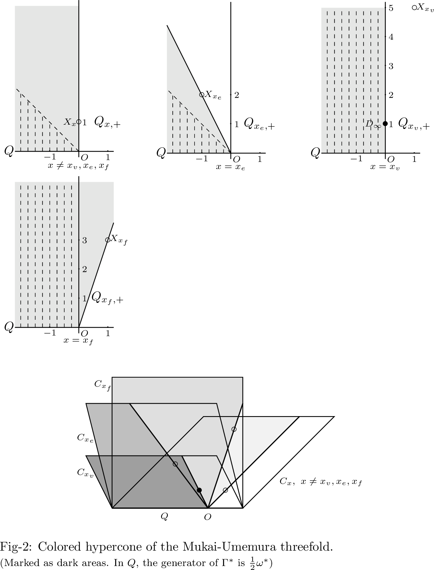 .
.
Now we compute anti-canonical divisors. By Theorem ?? , for each anti-canonical divisor \(\mathfrak a=\sum_{x\in \mathbb{P}^1}a_x\cdot x\) on \(\mathbb{P}^1\), there is a anti-canonical divisor \[\begin{align} \label{anti-can-div-mukai} \mathfrak d_\mathfrak a=\sum_{x\not= x_v,x_e,x_f}a_xX_{x}+(-4+5a_{x_v})X_{x_v}+(-1+2a_{x_e})X_{x_e}+(-2+3a_{x_f})X_{x_f}+a_{x_v}D_\infty \end{align}\tag{67}\] of \(X\), which is the divisor of a rational section of \(K_X^{-1}\) of weight \(2\omega\).
However, there is no effective divisor in 67 . In fact, it is showed in [48] that \[{\rm H}^0(X,K_X^{-1})\cong s^0\oplus s^{12},\] which implies \[{\rm H}^0(X,K_X^{-1})^{(B)}_{2\omega}=0.\] Also, [48] gives an effective divisor \[\mathfrak d_0=D_\infty\] on \(X\), which is the divisor of a \(G\)-invariant section in the component \(s^0\subset K_X^{-1}\). The divisor \(\mathfrak d_0\) can also be expressed as \[\mathfrak d_0=\mathfrak d_\mathfrak a-{\rm div}(e_{2\omega})\] with \[\mathfrak a=[x_v]+[x_f].\] Also by choosing \[\mathfrak a'=3[x_e]-[x_f],\] we get another effective anti-canonical divisor \[\mathfrak d_{\mathfrak a'}+5{\rm div}(e_{2\omega})=X_{x_v},\] which is the divisor of a section in \({\rm H}^0(X,K_X^{-1})^{(B)}_{12\omega}\subset s^{12}\).
For convenience, below we work with the divisor \(\mathfrak d_0\). Since it is \(G\)-invariant, we have \(\Delta_{\mathscr Z}(\mathfrak d_0)=\Delta_{\mathscr Z}(K_X^{-1})\) and \(A_x(\mathfrak d_0,\lambda)=A_x(K_X^{-1},\lambda-\kappa_P)\) for all \(x\). Set \(\lambda=k\omega\). We have \[\Delta_{\mathscr Z}(K_X^{-1})=\{k\omega|k\in\mathbb{Q},~0\leq k\leq 12\},\] and the data are listed in Table-1.2. The ploytopes \(\Delta^O_x(K_X^{-1})\) are drawn in Fig-3. Also, \[A(\mathfrak d_0,\lambda)=\min\{\frac{1}{60}k,1-\frac{1}{12}k\}.\]
| \(x\) | \(A_x(\mathfrak d,\lambda)\) | \(\mathbf{b}(\Delta_x^O(K_X^{-1}))-\kappa_P=(k,t)\) |
|---|---|---|
| \(x\not=x_e,x_v,x_f\) | \(0\) | \((\frac{69}{11},-\frac{31}{33})\) |
| \(x_e\) | \(-\frac14k\) | \((\frac{69}{11},\frac{149}{132})\) |
| \(x_v\) | \(\min\{1,\frac1{10}k\}\) | \((\frac{69}{11},-\frac34)\) |
| \(x_f\) | \(\frac16k\) | \((\frac{69}{11},-\frac{29}{22})\) |
Table-1.2: Data of \(K_X^{-1}\)
Figure 3: 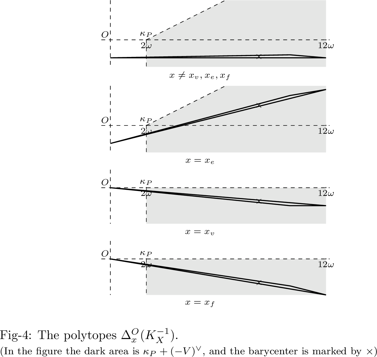 .
.
It is direct to check that ?? holds and \[(\kappa_P-\mathbf{b}(\Delta_{x}^O(K_X^{-1})))^\perp\cap \mathscr V_x=\{O\}\] for all \(x\). This implies that \(X\) is not \({\rm SL}_2\times{\rm k}^\times\)-spherical. Otherwise the \(\{\rm Id\}\times{\rm k}^\times\)-action would induce a non-trivial, \(G\)-equivariant product test configuration with zero Futaki invariant that is associated to some non-central \(v_0\in\mathscr V\). A contradiction. Thus by Theorem 1, \(X\) is \({\mathbf{G}}\)-uniform K-stable.
6.2 A completion of space of ordered triangles in \(\mathbb{P}^2\)↩︎
In this section we apply our results to study the equivariant uniform K-stability of a \(\mathbb{Q}\)-Fano quasihomogeneous \({\rm SL}_3\)-variety given by [12]. In the following we use the notations and conventions in [12]. Let \(G={\rm SL}_3\) and \(T\subset G\) the torus of diagonal matrixes. Then \(G/T\) is quasihomogeneous, which is referred as the space of ordered triangles in \(\mathbb{P}^2\). Choose \(B\) the group of upper triangular matrixes. Combinatorial data, in particular, the colours \(\mathscr D^B\), the lattice \(\Gamma\) and the embedding \(e\) of \(\Gamma\) into \(K^{(B)}\), and the valuation cone \(\mathscr V\) of \(G/H\) are established in [19] (see also [12]). We recall some of them for our later use.
As usual, for \(g=(g_{ij})\in G\), we choose \(\epsilon_i(g)=g_{ii}\), \(\omega_1 =\epsilon_1\), \(\omega_2 =\epsilon_1+\epsilon_2\) are the fundamental weights, and \(\alpha_1 =\epsilon_1-\epsilon_2\), \(\alpha_2 =\epsilon_2-\epsilon_3\) are the simple roots. Denote by \(\omega^\vee_i\) the fundamental coweights. Then for the weight lattice \(\Gamma\) we have \[\Gamma=\mathbb{Z}\alpha_1\oplus\mathbb{Z}\alpha_2.\]
The data of colours are listed as in Table-2.1 (according to the notation of [12]).
| Colour | \(x_D\) | \(v_D\) |
|---|---|---|
| \(D_x,~x\in\mathbb P^1\setminus\{x_1,x_2,x_3,\infty\}\) | \(x\) | \(q_x\) |
| \(D_\infty\) | \(\infty\) | \(q_\infty-(\omega_1^\vee+\omega_2^\vee)\) |
| \(D_{i},~i=1,2,3\) | \(x_i\) | \(q_{x_i}+\omega_2^\vee\) |
| \(\tilde D_{i},~i=1,2,3\) | \(x_i\) | \(q_{x_i}+\omega_1^\vee\) |
Table-2.1: Colours in \(G/H\)
Clearly, the associated parabolic subgroup \[P(G/H)={\rm Stab}_G(D_2)\cap{\rm Stab}_G(\tilde{D}_2)=B.\] Thus \(\kappa_P=2(\alpha_1+\alpha_2)\).
The valuation cone of \(G/H\) is given as following: an element \(a_1\omega_1^\vee+a_2\omega_2^\vee+hq_x\) is contained in \(\mathscr V_x\) if and only if \[\begin{align} (a_1,a_2,h)~\text{satisfies}~\left\{ \begin{aligned} &a_1,a_2\leq0\leq h,~\text{if}~x=x_1, x_2,x_3,\\ &a_1,a_2\leq-2h\leq0,~\text{if}~x=\infty,\\ &a_1,a_2\leq-h\leq0,~\text{otherwise}. \end{aligned} \right. \end{align}\]
We have the following completion of \(G/H\), \[X = \{(p_1, p_2, p_3, l_1, l_2, l_3)|p_j\in \mathbb{P}^2,~l_i \in \mathbb{P}^{2^*},~p_j \in l_i~\text{whenever}~i\not=j\}.\] Here \(G\) acts on \(\mathbb{P}^2\) via the tautological representation on \({\rm k}^3\) and on the dual space \(\mathbb{P}^{2^*}\) via the corresponding dual representation. Let us recall the list of \(G\)-orbits in \(X\) given in [12],
The open \(G\)-orbit of non-degenerate triangles.
The divisors \(W_i\), \(i=1,2,3\) which consists of degenerate triangles with \(p_j=p_k\) and \(l_j=l_k\), where \(\{i,j,k\}=\{1,2,3\}\).
The divisor \(\tilde{W}\) which consists of degenerate triangles with \(p_1\), \(p_2\), \(p_3\) collinear and \(l_1=l_2=l_3\).
The divisor \(W\) which consists of degenerate triangles with \(p_1=p_2=p_3\) and \(l_1\), \(l_2\), \(l_3\) pass through this point.
Codimension 2 orbits \(\tilde{Y}_i\) which consists of degenerate triangles with \(p_j=p_k\) and \(l_1=l_2=l_3\), where \(\{i,j,k\}=\{1,2,3\}\).
Codimension 2 orbits \(Y_i\) which consists of degenerate triangles with \(l_j=l_k\) and \(p_1=p_2=p_3\), where \(\{i,j,k\}=\{1,2,3\}\). It has codimension 3.
and
- A minimal \(G\)-germ (the closed orbit) \(Y\) which consists of degenerate triangles with \(p_1=p_2=p_3\) and \(l_1=l_2=l_3\).
Thus \(X = G\mathring X\), where \(\mathring X\) is the minimal \(B\)-chart of \(Y\) determined by the colored hypercone \(\mathscr C=\mathscr C(\mathscr W,\mathscr R)\) with \[\begin{align} \mathscr W=\{W,\tilde{W}, W_1,W_2,W_3\},~ \mathscr R=\{D_x|x\not=x_1,x_2,x_3\}, \end{align}\] where the \(G\)-valuations in \(\mathscr W\) are given in Table-2.2.
| Valuation | \(x_D\) | \(v_D\) |
|---|---|---|
| \(W\) | Central | \(-\omega_2^\vee\) |
| \(\tilde W\) | Central | \(-\omega_1^\vee\) |
| \(W_i,~i=1,2,3\) | \(x_i\) | \(q_{x_i}\) |
Table-2.2: \(G\)-valuations in \(\mathscr W\)
There is a \(G\)-equivariant small resolution of \(X\) (cf. [49] and [14]). By “small" we mean the exceptional locus has codimension at least 2 (it is showed in [49] that in case of \(X\) the exceptional locus has dimension 4). A small resolution is in particular crepant. This implies that \(X\) has klt singularities (cf. [44]).
By Theorem 32, there is a \(B\)-stable anti-canonical \(\mathbb{Q}\)-divisor \[\mathfrak d=W+\tilde{W}+\frac{2}{3}\sum_{i=1}^3(D_i+\tilde{D}_i+W_i),\] where the corresponding \(\mathfrak a=\frac{2}{3}([x_1]+[x_2]+[x_3])\). Choose the function \(f=f_0e_{-\alpha_1-\alpha_2}\in K^{(B)}_{-\alpha_1-\alpha_2}\), where \(f_0\in K^B\) with \({\rm div}(f_0)=\frac{2}{3}([x_1]+[x_2]+[x_3])-2[\infty]\) on \(\mathbb{P}^1\), it is direct to check by Theorem 15 that \(3\mathfrak d\) is an ample divisor on \(X\), which is the divisor of a section in \({\rm H}^0(X,K_X^{-3})^{(B)}_{3\kappa_P}\). It is showed that \(\Gamma=\mathbb{Z}\alpha_1\oplus\mathbb{Z}\alpha_2\). Choose a coordinate \(\lambda=\lambda_1\alpha_1+\lambda_2\alpha_2\) for \(\lambda\in\Gamma_\mathbb{Q}\). We have \[\Delta_\mathscr Z(\mathfrak d)=\{\lambda|2+2\lambda_1-\lambda_2\geq0,~2+2\lambda_2-\lambda_1\geq0,~2-\lambda_1-\lambda_2\geq0,~1-\lambda_1\geq0,~1-\lambda_2\geq0\}.\]
Figure 4: 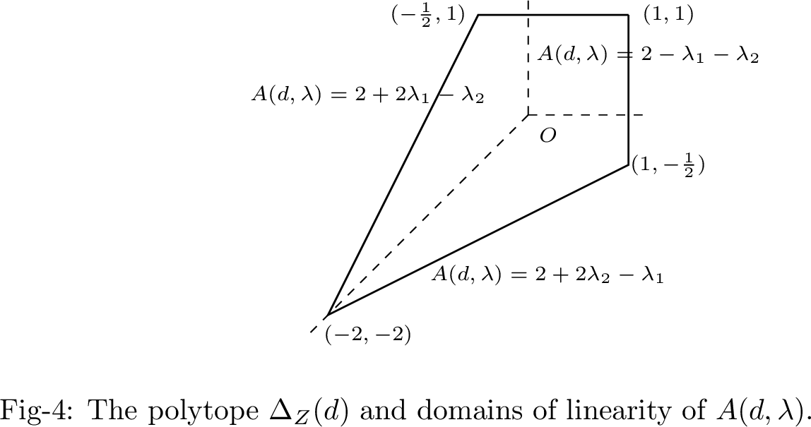 .
.
The functions \(\{A_x(\mathfrak d,\lambda):\Delta_\mathscr Z(\mathfrak d)|x\in C\}\), and barycenter of \(\Delta_x^O(K_X^{-1})\) are given in Table-2.3. The concave piecewise linear function \(A(\mathfrak d,\lambda)\) is marked in Fig-4.
| \(x\in\mathbb P^1\) | \(A_x(\mathfrak d,\lambda)\) | \(\mathbf{b}(\Delta_x^O(K_X^{-1}))-\kappa_P=(\lambda_1,\lambda_2,t)\) |
|---|---|---|
| \(x\in\mathbb P^1\setminus\{x_1,x_2,x_3,\infty\}\) | \(0\) | \((\frac{16141}{76706},\frac{16141}{76706},-\frac{12279}{27395})\) |
| \(\infty\in\mathbb P^1\) | \(-\lambda_1-\lambda_2\) | \((\frac{16141}{76706},\frac{16141}{76706},-\frac{5248}{191 765})\) |
| \(x_i,~i=1,2,3\) | \(\min\{\frac23+\lambda_1,\frac23+\lambda_2,\frac23\}\) | \((\frac{16141}{76706},\frac{16141}{76706},-\frac{166658}{575 295})\) |
Table-2.3: Data of \(K_X^{-1}\)
It is direct to check that ?? holds and \[(\kappa_P-\mathbf{b}(\Delta_{x}^O(K_X^{-1})))^\perp\cap \mathscr V_x=\{O\},~\forall x\in \mathbb{P}^1,\] which in particular implies that \(X\) can
not be \(G\times{\rm k}^\times\)-spherical again. By Theorem 1, we have
Proposition 54. The \(\mathbb{Q}\)-Fano variety \(X\) is \({\mathbf{G}}\)-uniformly K-stable.
7 Appendix↩︎
7.1 Lemmas on colours in spherical homogeneous spaces↩︎
The following lemma is a combination of several known results (cf. [12] and [50]), we include it here for readers’ convenience.
Lemma 55. Let \(G/H\) be a spherical homogeneous space and \(\sigma\in {\rm Aut}_G(G/H)\) a \(G\)-equivariant isomorphism. Suppose that two different colours \(D\) and \(D'\) satisfies \(D=\sigma(D')\). Then both \(D\) and \(D'\) are of type-a, and there is a simple root \(\alpha\in\Pi_G\) so that \(\mathscr D^B(G/H;\alpha)=\{D,D'\}\). Moreover, \(v_D=v_{D'}\) in the hyperspace of \(G/H\).
Proof. It is obvious that if \(D\in\mathscr D^B(G/H;\alpha)\), then so is \(D'\). Thus \(\#\mathscr D^B(G/H;\alpha)\geq2\). This is possible only if both \(D\) and \(D'\) are of type-a (cf. [12]), and \(\mathscr D^B(G/H;\alpha)=\{D,D'\}\). For the last point it suffices to show that for any \(e_\lambda\in{\rm k}(G/H)^{(B)}_\lambda\), \[{\rm ord}_D(e_\lambda)={\rm ord}_{D'}(e_\lambda).\] Since \(\sigma\) commutes with the \(G\)-action, \(\sigma\cdot e_\lambda\in{\rm k}(G/H)^{(B)}_\lambda\). Hence \(\sigma\cdot e_\lambda=c e_\lambda\) for some constant \(c\not=0\), and \[{\rm ord}_D(e_\lambda)={\rm ord}_{\sigma(D')}(e_\lambda)={\rm ord}_{D'}(\sigma^{-1}\cdot e_\lambda)={\rm ord}_{D'}(e_\lambda),\] which concludes the Lemma. ◻
Lemma 56. Let \((X,L)\) be a polarized \(G\)-spherical variety and \(\mathfrak d=\sum_{D\in\mathscr B(X)}m_DD\) a divisor of \(L\), which is the divisor of some \(B\)-semiinvariant rational section \(s\) of \(L\) with \(B\)-weight \(\lambda_0\). Suppose that \(D\in\mathscr D^B(X;\alpha)\) is a colour of type-a’ or b that corresponds to a simple root \(\alpha\in\Pi_G\). Then \(\alpha^\vee(\lambda_0)=m_D\), and for any \(\lambda\in\Gamma_\mathbb{Q}\) so that \(v_D(\lambda)+m_D=0\), it holds \[\langle\alpha^\vee,\lambda+\lambda_0\rangle=0.\]
Proof. Let \(G/H\) be the spherical homogeneous space that is embedded in \(X\). Then for each \(D\in\mathscr D^B\), there is a line bundle \(L_D\) on \(G/H\) so that \(D={\rm div}(s_D)\) for some \(s_D\in{\rm H}^0(G/H,L_D)^{(B)}_{\lambda_D}\), where \(\lambda_D\) is the \(B\)-weight of \(s_D\). Since \((\mathfrak d-\sum_{D\in\mathscr D^B}m_DD)|_{G/H}=0\), we have \[f:=\frac{s|_{G/H}}{\prod_{D\in\mathscr D^B}s_D^{m_D}}\in\mathscr O(G/H)^\times.\] By [51], \(G\)-acts on \(f\) through a character \(\lambda_G\in\mathfrak X(G)\). Consequently, \[\lambda_0=\sum_{D\in\mathscr D^B}m_D\lambda_D+\lambda_G.\] Let \(\alpha\) be a simple root in \(\Pi_G\). It holds \[\begin{align} \langle\alpha^\vee,\lambda_0\rangle=\sum_{D\in\mathscr D^B}m_D\langle\alpha^\vee,\lambda_D\rangle =\sum_{D\in\mathscr D^B(X;\alpha)}m_D\langle\alpha^\vee,\lambda_D\rangle. \end{align}\]
When \(\alpha\) is of type-a’, \(\mathscr D^B(X;\alpha)\) contains precisely one colour (denoted by \(D\)), and by [52] (see also [40] or [12]), \[\langle\alpha^\vee,\lambda_0\rangle=m_D\langle\alpha^\vee,\lambda_D\rangle=2m_D.\] Combining with the fact that \(v_D=\frac{1}{2}\alpha^\vee|_\Gamma\) for the type-a’ colour \(D\), we get the Lemma.
When \(\alpha\) is of type-b, again \(\mathscr D^B(X;\alpha)\) contains only one colour (denoted by \(D\)), similarly as above, \[\langle\alpha^\vee,\lambda_0\rangle=m_D\langle\alpha^\vee,\lambda_D\rangle=m_D.\] Combining with the fact that \(v_D=\alpha^\vee|_\Gamma\) for the type-b colour \(D\), we get the Lemma. ◻
7.1.1 A combinatorial property of \(B\)-stable ample divisors↩︎
Let \((X,L)\) be a polarized \(G\)-variety of complexity 1, and \[\mathfrak d=\sum_{D\in\mathscr B(X)}m_DD\] a divisor of \(L\), which is the divisor of some \(B\)-semiinvariant rational section \(s\) of \(L\) with \(B\)-weight \(\lambda_0\). We have
Lemma 57. Suppose that
- \(X\) is a one-parameter \(G\)-variety and \(D\in\mathscr D^B(\alpha)\) a colour of type-a’ or b,
or
- \(X\) is a quasi-homogeneous \(G\)-variety and \(D\) a central colour that descends to a type-a’ or b colour in \(\mathscr D^B(\alpha)\) on \(Z'\) in the proof of Theorem 32.
Then \[\langle\alpha^\vee,\lambda+\lambda_0\rangle=0,\] whenever \(\lambda\in\Gamma_\mathbb{Q}\) satisfies \(v_D(\lambda)+m_D=0\).
Proof. We start with case (1) when \(X\) is a one-parameter \(G\)-variety. In this case a general \(G\)-orbit in \(X\) is isomorphic to some spherical homogeneous space \(O\). For simplicity we denote by \(O\) any fixed such an orbit. Recall that \(\Gamma\cong\Gamma(O)\). Let \(D\in\mathscr D^B\) be a colour of \(X\) of type-a’ or b. Then from the construction in Section 3.1.1 and Lemma 55, \(D\cap O=\hat{D}\) is a single colour of \(O\) which has the same type with \(D\), and satisfies \(v_D=v_{\hat{D}}\). By restricting \(L\) and \(s\) on \(O\), we get \(s|_O\) a \(B\)-semiinvariant section of \(L|_O\) with the same weight \(\lambda_0\) and \(\mathfrak d|_O\) its divisor. The statement then follows from Lemma 56.
Now we turn to case (2). Assume that \(X\) is quasihomogeneous which contains a homogeneous space \(G/H\). Then for any colour \(D\), \(D\cap(G/H)\) is the divisor of a \(B\)-semiinvariant section \(s_D\in{\rm H}^0(G/H,L_D)^{(B)}_{\lambda_D}\) for some \(\lambda_D\in \mathfrak X(B)\). Recall the set \(C^o\) constructed in Section 3.2 above. We claim that \[\lambda_{X_z}\equiv\lambda^o~\text{(modulo a G-character)}\] for some \(\lambda^o\in\mathfrak X(B)\) for any \(X_z\) with \(z\in C^o\). Note for any \(z_1,z_2\in\mathring C\), the difference of the colours \(X_{z_1}-X_{z_2}\) coincides with the divisor of a \(B\)-invariant function \(f_0:=\frac{z-z_1}{z-z_2}\in{\rm k}(\mathbb{P}^1)\cong{\rm k}(X)^B\). This implies \[f':=\frac{s_{X_{z_1}}}{f_0s_{X_{z_2}}}\in\mathscr O(G/H)^\times.\] By [51], \(G\) acts on \(f'\) through some character \(\mu\), whence \[\lambda_{X_{z_1}}=\lambda_{X_{z_2}}+\mu,\] and we get the claim.
By restricting \(s\) on \(G/H\), we get \[f=\frac{s|_{G/H}}{\prod_{D\in\mathscr D^B}s_D^{m_D}}\in\mathscr O(G/H)^\times.\] Again by [51], we can decompose \[\lambda_0=m\lambda^o+\lambda_0'+\lambda_0''+\lambda_G,\] where \(m=\sum_{z\in C^o}m_{X_z}\in\mathbb{N}_+\), \(\lambda_0'=\sum_{D\in\mathscr D^B\setminus\mathscr B(X)^{P'}}m_D\lambda_D\) (every \(D\) appears in this sum descends to a colour of \(Z'\)), \(\lambda_0''=\sum_{D\in(\mathscr D^B)^{P'},x_D\not\in C^o}m_D\lambda_D\) (every \(D\) in this sum descends to a \(L_{P'}\)-stable divisor in \(Z'\)), and \(\lambda_G\in\mathfrak X(G)\). In particular, \(\lambda^o\) and \(\lambda_0''\) are \(L_{P'}\)-characters, since \(P'\) stabilizes \(X_z\) for \(z\in C^o\) and any \(D\in(\mathscr D^B)^{P'}\). Thus, \[\langle\alpha^\vee,\lambda_0\rangle=\langle\alpha^\vee,\lambda_0'\rangle,~\forall\alpha\in\Pi_{L_{P'}}.\] On the other hand, for a colour \(D\) that descends to a colour \(D'\) of type-a’ or b in \(Z'\), \(v_D=\frac{1}{2}\alpha^\vee|_{\Gamma}\) or \(\alpha^\vee|_\Gamma\) for \(\alpha\in\Pi_{L_{P'}}\). The Lemma then follows from the previous case. ◻
7.2 Lemmas on one-parameter \(G\)-varieties of type↩︎
Lemma 58. Let \(X\) be a one-parameter \(G\)-variety of type and \(\mathcal{O}\) any \(G\)-orbit in it. Then the coloured cone \((\mathscr C,\mathscr R)\) of \(\mathcal{O}\) can not be totally contained in \(\mathscr Q\).
Proof. Note that any \(G\)-orbit in general position is spherical. By [53] any \(G\)-orbit is spherical. Also \(X_\mathcal{O}:=\overline{\mathcal{O}}\) is normal by [12], whence a spherical variety. In particular \(X_\mathcal{O}\) contains only finitely many \(G\)-orbits by Akhiezer’s theorem [54]. Thus there are only finitely many coloured cones in the fan \(\mathfrak F_X\) of \(X\) whose relative interior intersects \(\mathscr V\) and contains \((\mathscr C,\mathscr R)\) as a face.
Denote by \(C\) the smooth projective curve so that \({\rm k}(X)^G={\rm k}(C)\). If \((\mathscr C,\mathscr R)\subset\mathscr Q\), then for almost every \(x\in C\), \(({\rm Cone}(q_x,\mathscr C),\mathscr R)\) is a coloured cone in \(\mathfrak F_X\). Also \({\rm RelInt}(\mathscr C)\cap\mathscr V\not=\emptyset\) since \((\mathscr C,\mathscr R)\) is the coloured cone of a \(G\)-subvariety, which implies \({\rm RelInt}({\rm Cone}(q_x,\mathscr C))\cap\mathscr V\not=\emptyset\) for those \(x\in C\) above. Thus \(X_\mathcal{O}\) contains infinitely many \(G\)-orbits. A contradiction. ◻
The following Lemma is a special case of a general result [12]. We include an elementary proof below in our case only for readers’ convenience.
Lemma 59. Let \(X\) be a one-parameter \(G\)-variety of type and \(C\) the smooth projective curve so that \({\rm k}(X)^G={\rm k}(C)\). Then the rational quotient \({\rm pr}_B:X\dashrightarrow C\) is a morphism \({\rm pr}_B:X\to C\) separating general \(G\)-orbits.
Proof. Suppose that \(\mathring X\subset X\) is any \(B\)-chart given by the coloured data \((\mathscr W,\mathscr R)\). Then there is an open subset \(X^o\subset\mathring X\) where \({\rm pr}_B\) is defined. By definition, for any \(x\in C\), \({\rm pr}_B^{-1}(x)\cap X^o\) is the union of all \(D\cap X^o\), where \(D\in\mathscr W\sqcup\mathscr R\) so that \(x_D=x\) and \(h_D>0\). We hope to show under our assumptions, \({\rm pr}_B\) in fact can be extended to the whole \(X\).
By Lemma 58, for any \(G\)-orbit \(\mathcal{O}\subset X\), there is a unique \(x\in C\) so that the coloured cone of \(X_\mathcal{O}\subset\mathscr Q_{x,+}\). Thus there is a \(G\)-invariant map \[{\rm Pr}: X\to C\] that maps any point in \(\mathcal{O}\) to \(x\in C\). This is a map globally defined on \(X\), and \({\rm Pr}|_{X^o}={\rm pr}_B|_{X^o}\). It suffices to show that \({\rm Pr}\) is regular on the whole \(X\).
Suppose that \((\mathscr C,\mathscr R)\) is a hypercone of type so that each \((\mathscr C_x,\mathscr R_x)\), \(x\in C\) is a coloured cone in \(\mathscr F_X\). As in [25], [27] we denote the locus of \((\mathscr C,\mathscr R)\) by \({\rm Loc}(\mathscr C,\mathscr R):=\{x\in C|(\mathscr C_x,\mathscr R_x)\not\subset\mathscr Q\}\). Denote by \(U(\mathscr C,\mathscr R)\) the corresponding \(B\)-chart defined by \((\mathscr C,\mathscr R)\). Note that \(h_D\geq0\) for any \(D\in\mathscr B(X)\). For any affine subset \(\mathring C\subset C\), \({\rm k}[\mathring C]\subset{\rm k}(C)={\rm k}(X)^G\) is contained in \({\rm k}[U(\mathscr C,\mathscr R)]\) if and only if \({\rm Loc}(\mathscr C,\mathscr R)\subset \mathring C\). On the other hand, since every \(f\in{\rm k}[\mathring C]\) is \(G\)-invariant, \(f\) is regular on the \(G\)-span of \(U(\mathscr C,\mathscr R)\) if and only if \(f\in{\rm k}[U(\mathscr C,\mathscr R)]\). Then \({\rm Pr}\) is regular on the \(G\)-span of every \(U(\mathscr C,\mathscr R)\) so that \({\rm Loc}(\mathscr C,\mathscr R)\subset \mathring C\), and is a globally defined morphism. ◻
7.3 Lemmas on counting integral points↩︎
Lemma 60. Suppose there are \(m\) numbers \(\alpha_1,...,\alpha_m\in\mathbb{R}\) so that \[\begin{align} \label{sum-cond-si} \sum_{i=1}^m\alpha_i\geq0>\sum_{i=1}^m[\alpha_i]. \end{align}\qquad{(26)}\] Then \[\begin{align} \label{sum-cond-estimate} m>\sum_{i=1}^m\alpha_i\geq0>\sum_{i=1}^m[\alpha_i]>-m. \end{align}\qquad{(27)}\]
Proof. Note that \[\alpha_i=[\alpha_i]+\{\alpha_i\},~i=1,...,m.\] From the right-hand side inequality of ?? we have \[m>\sum_{i=1}^m\{\alpha_i\}>\sum_{i=1}^m\alpha_i\geq0.\] At the same time, the left-hand side inequality of ?? yields \[\sum_{i=1}^m[\alpha_i]\geq-\sum_{i=1}^m\{\alpha_i\}>-m.\] Hence we get the Lemma. ◻
From the above Lemma we get the following estimates
Lemma 61. Let \(\mathfrak d_0\) be an ample divisor given by 7 . Set \[\mathfrak T_k:=\{\lambda\in\Delta_\mathscr Z(\mathfrak d_0)\cap\frac{1}{k}\Gamma|\sum_{x\in C}[kA_x(\mathfrak d_0,\lambda)]<0\},~k\in\mathbb{N}_+.\] Then there is a \(k_0\in\mathbb{N}_+\) depends only on \(\mathfrak d_0\), and constants \(c,c'>0\) so that the cardinal number \(\#\mathfrak T_k\leq ck^{r-1}\) for any \(k\in\mathbb{N}_{\geq k_0}\), and \[-c'<\sum_{x\in C}[kA_x(\mathfrak d_0,\lambda)]<kA(\mathfrak d_0,\lambda)<c', ~\forall k\in\mathbb{N}_{\geq k_0}~\text{and}~\lambda\in\mathfrak T_k.\]
Proof. Note that there are only finitely many points \(x_1,...,x_m\in C\) so that \(A_{x_i}(\mathfrak d_0,\lambda)\not\equiv0\) for \(i=1,...,m\). Take \(\alpha_i=kA_{x_i}(\mathfrak d_0,\lambda)\). By Lemma 60, \[\begin{align} \label{neg-set} \mathfrak T_k\subset\{\lambda\in\Delta_\mathscr Z(\mathfrak d_0)\cap\frac{1}{k}\Gamma|A(\mathfrak d_0,\lambda)<\frac{m}{k}\}. \end{align}\tag{68}\] On the other hand, the piecewise linear function \(A(\mathfrak d_0,\lambda)>0\) on \(\Delta_\mathscr Z(\mathfrak d_0)\). Thus there is a \(k_0\in\mathbb{N}_+\) that depends only on \(\mathfrak d_0\) (more precisely, the integer \(m\), the function \(A(\mathfrak d_0,\lambda)\), and the shape of \(\Delta_\mathscr Z(\mathfrak d_0)\) which are completely determined by \(\mathfrak d_0\)) such that the right-hand side of 68 is contained in a strip near the boundary of \(\Delta_\mathscr Z(\mathfrak d_0)\) with facets parallel to that of the boundary. It is also direct to check that for \(k\geq k_0\), this strip can be chosen so that its width \(\leq\frac{c_0m}{k}\), where \(c_0>0\) is again a constant that depends only on the function \(A(\mathfrak d_0,\lambda)\) and the shape of \(\Delta_\mathscr Z(\mathfrak d_0)\). In particular, \(c_0\) is independent of \(k\in\mathbb{N}_+\). Thus \(\#\mathfrak T_k\leq ck^{r-1}\) for some uniform \(c>0\). The last point follows from ?? by taking \(c'=m\). ◻
The following Lemma can be derived from a general result of Pukhlikov-Khovanskij [55]. We include it here for reads’ convenience.
Lemma 62. Let \(\mathfrak M\cong \mathbb{Z}^r\) be a lattice and \(\Delta\subset \mathfrak M_\mathbb{R}\) be a solid, integral convex polytope in it. Let \(\pi:\Delta\to\mathbb{R}\) be a monomial of degree \(d\) on \(\mathfrak M_\mathbb{R}\) and \(f:\Delta\to\mathbb{R}\) a concave, piecewise linear function whose domains of linearity \(\{\Omega_a\}_{a=1}^{N_f}\) consist of integral polytopes in \(\Delta\). Suppose that on each domain of linearity \(\Omega_a\), \[f(\lambda)=\frac{1}{p_a}(q_a(\lambda)+r_a),\] where \((p_a,-q_a)\in\mathbb{Z}\oplus\mathbb{Z}\) is a primitive vector, \(r_a\in\mathbb{Q}\), and \(f\) takes integral value at every vertex f its domains of linearity. Define \[S_k(f;\pi):=\sum_{\lambda\in k\Delta\cap\mathfrak M}[kf(\frac{\lambda}{k})]\pi(\lambda),~k\in\mathbb{N}_+.\] Then \[\begin{align} S_k(f;\pi)=&k^{r+d+1}\int_{\Delta}f(\lambda)\pi(\lambda)d\lambda+\frac{1}{2}k^{r+d}\int_{\partial\Delta}f(\lambda)\pi(\lambda)d\sigma\notag\\ &-\frac{1}{2}k^{r+d}\sum_{a=1}^{N_f}\int_{\Omega_a}(1-\frac{1}{|p_a|})\pi(\lambda)d\lambda+O(k^{r+d-1}),~k\to+\infty. \end{align}\] where \(d\sigma\) is the induced lattice measure on \(\partial\Delta\).
Proof. Since \(f\) is concave, \(\min_\Delta f\) is attained at some vertex of \(\Delta\). Hence \(\min_\Delta f\in\mathbb{Z}\). Consider a convex polytope \[\Delta_m:=\{(t,\lambda)|\lambda\in\Delta,~t\in\mathbb{R},~\min_\Delta f\leq t\leq f(\lambda)\}.\] Then \(\Delta_m\) is an \((r+1)\)-dimensional convex integral polytope in \(\mathfrak M_\mathbb{R}\oplus\mathbb{R}\). Clearly, \[\begin{align} [kf(\frac{\lambda}{k})]=&[k(f(\frac{\lambda}{k})-\min_\Delta f)]+k\min_\Delta f\notag\\ =&\#\{(\{\frac{1}{k}\lambda\}\times\frac{1}{k}\mathbb{Z})\cap\Delta_m\}+k\min_\Delta f-1. \end{align}\] Thus \[\begin{align} \label{1st-term1-end-lemma-app} \sum_{\lambda\in k\Delta\cap\mathfrak M}[kf(\frac{\lambda}{k})]\pi(\lambda)=&\sum_{(\lambda,t)\in\Delta_m\cap\frac{1}{k}(\mathfrak M\oplus\mathbb{Z})}\pi(k\lambda)+(k\min_\Delta f-1)\sum_{\lambda\in\Delta\cap\frac{1}{k}\mathfrak M}\pi(k\lambda)\notag\\ =&k^d\sum_{(\lambda,t)\in\Delta_m\cap\frac{1}{k}(\mathfrak M\oplus\mathbb{Z})}\pi(\lambda)+k^d(k\min_\Delta f-1)\sum_{\lambda\in\Delta\cap\frac{1}{k}\mathfrak M}\pi(\lambda). \end{align}\tag{69}\] By [55], the first term \[\begin{align} \label{1st-term1-lemma-app} \sum_{(\lambda,t)\in\Delta_m\cap\frac{1}{k}(\mathfrak M\oplus\mathbb{Z})}\pi(\lambda)=&k^{r+1}\int_{\Delta_m}\pi(\lambda)dt\wedge d\lambda+\frac{1}{2}k^r\int_{\partial\Delta_m}\pi(\lambda)d\bar\sigma+O(k^{r-1}),~k\to+\infty, \end{align}\tag{70}\] where \(d\bar\sigma\) is the induced lattice measure on \(\partial\Delta_m\). We have \[\begin{align} \label{main-term-lemma-app} \int_{\Delta_m}\pi(\lambda)dt\wedge d\lambda=\int_{\Delta}(f(\lambda)-\min_\Delta f)\pi(\lambda)d\lambda. \end{align}\tag{71}\] The boundary \(\partial\Delta_m\) consists of three parts: On \(F_1:=(\mathbb{R}\times\partial\Delta)\cap\Delta_m\), \[\begin{align} \label{bdry-term1-lemma-app} \int_{F_1}\pi(\lambda)d\bar\sigma=\int_{\partial\Delta}(f(\lambda)-\min_\Delta f)\pi(\lambda)d\sigma, \end{align}\tag{72}\] where \(d\sigma\) is the induced lattice measure on \(\partial\Delta\). On \(F_2=\{\min_\Delta f\}\times \Delta\), \[\begin{align} \label{bdry-term2-lemma-app} \int_{F_2}\pi(\lambda)d\bar\sigma=\int_{\Delta}\pi(\lambda)d\bar\sigma. \end{align}\tag{73}\] On \(F_3=\{\text{graph of}~f\}\), since \(f\) is rational, on each domain of linearity \(\Omega\) where \[f(\lambda)=\frac{1}{p}(q(\lambda)+r')\] for primitive vector \((p,-q)\in\mathbb{Z}\oplus\mathbb{M}^*\) and \(r'\in\mathbb{Q}\), \[\begin{align} \label{bdry-term3-lemma-app} \int_{\text{graph f on}~\Omega}\pi(\lambda)d\bar\sigma=\int_{\Omega}\pi(\lambda)\frac{1}{|(p,-q)|}d\sigma_0 =\frac{1}{|p|}\int_{\Omega}\pi(\lambda)d\lambda. \end{align}\tag{74}\] Here \(d\sigma_0=\sqrt{1+\frac{|q|^2}{p^2}}d\lambda\) is the standard induced Lebesgue measure. Plugging 71 74 into 70 , we get \[\begin{align} \sum_{(\lambda,t)\in\Delta_m\cap\frac{1}{k}(\mathfrak M\oplus\mathbb{Z})}\pi(\lambda)=&k^{r+1}\int_{\Delta}(f(\lambda)-\min_\Delta f)\pi(\lambda)d\lambda+\frac{1}{2}k^r\int_{\partial\Delta}(f(\lambda)-\min_\Delta f)\pi(\lambda)d\sigma\notag\\ &+\frac{1}{2}k^r\sum_{a=1}^{N_f}\int_{\Omega_a}(1-\frac{1}{|p_a|})\pi(\lambda)d\lambda+O(k^{r-1}),~k\to+\infty. \end{align}\] Similarly, \[\begin{align} \sum_{\lambda\in\Delta\cap\frac{1}{k}\mathfrak M}\pi(\lambda)=&k^{r}\int_{\Delta}\pi(\lambda)d\lambda+\frac{1}{2}k^{r-1}\int_{\partial\Delta}\pi(\lambda)d\sigma+O(k^{r-2}),~k\to+\infty. \end{align}\] Plugging the above two relations into 69 we get the Lemma. ◻
7.4 An alternative proof to Theorem 48↩︎
In the following we give an alternative proof of via an intersection formula of the Futaki invariant (cf. [3], [23]). Given a normal test configuration \((\mathcal{X},\mathcal{L})\) of \((X,L)\), the Futaki invariant can also be interpreted as intersection numbers \[\begin{align} \label{Fut-def-int} {\rm Fut}(\mathcal{X},\mathcal{L})=\frac{1}{V}K_{\mathcal{X}/\mathbb{P}^1}\cdot\mathcal{L}^{\cdot n}+\frac{\bar S}{V(n+1)}\mathcal{L}^{\cdot(n+1)}, \end{align}\tag{75}\] where \(V=L^n\) is the volume of \((X,L)\), \(\bar S\) the mean value of the scalar curvature of \((X,L)\), and \[\begin{align} K_{\mathcal{X}/\mathbb{P}^1}=K_{\mathcal{X}}-{\rm pr}^*K_{\mathbb{P}^1} \end{align}\] a Weil divisor on \(\mathcal{X}\).
Assume that \((X,L)\) is a polarized spherical variety with \(L\) has a divisor \(\mathfrak d_0\) given by 7 , and \[\mathfrak d_K=\sum_{D\in\mathscr B(X)}\bar m_DD\] a \(B\)-stable anti-canonical divisor of \(X\) corresponds to weight \(\kappa_P\). Let \((\mathcal{X},\mathcal{L})\) be a normal test configuration associated to \(v_0\in\mathcal{Q}_{x_0,+}\) and \(m=-1\). Without loss of generality we may also assume that \(\mathcal{L}\) has a divisor \(\mathfrak D\) given by 25 with \(r_0=1\) and \(m_\infty=0\) (otherwise one needs to divide 75 by \(r_0^{n+1}\)). Then by Theorems 29 (in the one-parameter case) and 32 (in the quasihomogeneous case), it is direct to see \[\begin{align} \mathfrak d_{\mathcal{X}/\mathbb{P}^1}=-\sum_{D\in\mathscr B(X)}\bar m_D\overline{D}-h_0(a_{x_0}-1)\mathcal{X}_0. \end{align}\] In particular, if \(X\) is \(\mathbb{Q}\)-Fano and \(K=K_X^{-1}\), we can take \(\mathfrak d_K=\mathfrak d_0\) (in particular, \(\bar m_D=m_D\) for all \(D\in\mathscr B(X)\)) and \[\mathfrak d_{\mathcal{X}/\mathbb{P}^1}=-(\mathfrak D+(h_0(a_{x_0}-1)-m_0){\rm pr}^*([0]))\] is also a \(\mathbb{Q}\)-Cartier divisor that corresponds to the weight \(-\kappa_P\).
The line bundle \[\begin{align} \mathcal{L}_\epsilon:=\mathcal{L}+\epsilon K_{\mathcal{X}/\mathbb{P}^1} \end{align}\] is a \(\mathbb{Q}\)-line bundle on \(\mathcal{X}\), and is ample when \(0<\epsilon\ll1\). The divisor \[\begin{align} \mathfrak D_\epsilon:=\mathfrak D+\epsilon \mathfrak d_{\mathcal{X}/\mathbb{P}^1}=\sum_{D\in\mathscr B(X)}(m_D-\epsilon m_D)\overline{D}+(m_0-\epsilon(a_{x_0}-1))\mathcal{X}_0 \end{align}\] is a divisor of \(\mathcal{L}_\epsilon\) corresponds to weight \((1-\epsilon)\kappa_P\), and the associated function is \[\begin{align} \tilde{A}_{x}^\epsilon(\lambda,t):=\left\{\begin{aligned}&(1-\epsilon)\min\{A_{x_0}(\mathfrak d,\frac{\lambda{1-\epsilon}}{)},\frac{-t+m_0-\epsilon h_0(a_{x_0}-1)+\ell_0(\lambda)}{h_0(1-\epsilon)}\},~\text{when}~x=x_0,\\ &(1-\epsilon)A_{x}(\mathfrak d,\frac{\lambda}{1-\epsilon}),~\text{when}~x\not=x_0,\end{aligned}\right. \end{align}\] for \(\lambda\in\Gamma_\mathbb{R}\) and \(\tilde{A}^\epsilon(\lambda,t)=\sum_{x\in C}\tilde{A}_{x}^\epsilon(\lambda,t)\). The polytope \[\begin{align} \label{Delta-eps} \tilde{\Delta}_\mathscr Z^\epsilon(\mathfrak D_\epsilon)=&\{(\lambda,t)|\tilde{A}^\epsilon(\lambda,t)\geq0\}\notag\\ =&\{(\lambda,t)|\lambda\in(1-\epsilon)\Delta_\mathscr Z(\mathfrak d_0),~0\leq t\leq\tau^0_\epsilon(\lambda)\}, \end{align}\tag{76}\] where \[\begin{align} \tau^0_\epsilon(\lambda)=m_0-\epsilon h_0(a_{x_0}-1)+\ell_0(\lambda)+h_0(1-\epsilon)(A(\frac{\lambda{1-\epsilon}}{)}-A_{x_0}(\frac{\lambda{1-\epsilon}}{)}). \end{align}\] Set \[\begin{align} \tilde{\tau}^0_\epsilon(\lambda)=m_0-\epsilon h_0(a_{x_0}-1)+\ell_0(\lambda)-h_0(1-\epsilon)A_{x_0}(\frac{\lambda{1-\epsilon}}{)}. \end{align}\] Then for \(\lambda\in\Gamma_\mathbb{R}\), \[\begin{align} \label{A-x-eps-piece} \tilde{A}^\epsilon(\lambda,t):=\left\{\begin{aligned} &(1-\epsilon)A(\mathfrak d_0,\frac{\lambda}{1-\epsilon}),~\text{when}~0\leq t\leq\tilde{\tau}_0^\epsilon(\lambda),\\ &(1-\epsilon)\sum_{x\not=x_0}A_{x}(\mathfrak d_0,\frac{\lambda}{1-\epsilon})+\frac{m_0-\epsilon h_0(a_{x_0}-1)-t+\ell_0(\lambda)}{h_0},~\text{when}~\tilde{\tau}^0_\epsilon(\lambda)\leq t\leq\tau^0_\epsilon(\lambda).\end{aligned}\right. \end{align}\tag{77}\]
Note that when \(\epsilon\in\mathbb{Q}\), \[\mathcal{L}_\epsilon^{\cdot(n+1)}=\mathcal{L}^{\cdot(n+1)}+(n+1)\epsilon K_{\mathcal{X}/\mathbb{P}^1}\cdot \mathcal{L}^{\cdot n}+O(\epsilon^2),~\epsilon\to0^+.\] Apply the intersection formula [14] to \(\mathcal{L}_\epsilon\), we get \[\begin{align} \label{mathcal-L-n431} \mathcal{L}^{\cdot(n+1)}=&(n+1)!\int_{\tilde{\Delta}_\mathscr Z(\mathfrak D)}\tilde{A}(\lambda,\tau)\pi(\lambda+\kappa_P) d\lambda\wedge d\tau\notag\\ =&(n+1)!\int_{\Delta_\mathscr Z(\mathfrak d_0)}\int_{0}^{\tau^0(\lambda)}\tilde{A}(\lambda,\tau)\pi(\lambda+\kappa_P) d\lambda\wedge d\tau, \end{align}\tag{78}\] and \[\begin{align} \label{KX47P-term} K_{\mathcal{X}/\mathbb{P}^1}\cdot \mathcal{L}^{\cdot n}&=\frac{1}{n+1}\left.\frac{d}{d\epsilon}\right|_{\epsilon=0}\mathcal{L}_\epsilon^{\cdot(n+1)}\notag\\ &=n!\left.\frac{d}{d\epsilon}\right|_{\epsilon=0}\int_{\tilde{\Delta}_\mathscr Z^\epsilon(\mathfrak D_\epsilon)}\tilde{A}^\epsilon(\lambda,\tau)\pi(\lambda+(1-\epsilon)\kappa_P) d\lambda\wedge d\tau. \end{align}\tag{79}\] By 76 and 77 , \[\begin{align} &\int_{\tilde{\Delta}_\mathscr Z^\epsilon(\mathfrak D_\epsilon)}\tilde{A}^\epsilon(\lambda,\tau)\pi(\lambda+(1-\epsilon)\kappa_P) d\lambda\wedge d\tau\notag\\ =&\int_{(1-\epsilon)\Delta_\mathscr Z(\mathfrak d_0)}\int_{0}^{\tilde{\tau}^0_\epsilon(\lambda)}(1-\epsilon)A(\mathfrak d_0,\frac{\lambda}{1-\epsilon})\pi(\lambda+(1-\epsilon)\kappa_P) d\lambda\wedge dt\notag\\ &+\int_{(1-\epsilon)\Delta_\mathscr Z(\mathfrak d_0)}\int_{\tilde{\tau}^0_\epsilon(\lambda)}^{\tau^0_\epsilon(\lambda)}(1-\epsilon)\sum_{x\not=x_0}A_x(\mathfrak d_0,\frac{\lambda}{1-\epsilon})\pi(\lambda+(1-\epsilon)\kappa_P) d\lambda\wedge dt\\ &+\int_{(1-\epsilon)\Delta_\mathscr Z(\mathfrak d_0)}\int_{\tilde{\tau}^0_\epsilon(\lambda)}^{\tau^0_\epsilon(\lambda)}\frac{m_0-\epsilon h_0(a_{x_0}-1)-t+\ell_0(\lambda)}{h_0}\pi(\lambda+(1-\epsilon)\kappa_P) d\lambda\wedge dt. \end{align}\] Using change of variables \(\lambda\to(1-\epsilon)\lambda\), \(t\to(1-\epsilon)t\), and the relation 10 , we can rewrite the first two terms as \[\begin{align} &\int_{(1-\epsilon)\Delta_\mathscr Z(\mathfrak d_0)}\int_{0}^{\tilde{\tau}^0_\epsilon(\lambda)}(1-\epsilon)A(\mathfrak d_0,\frac{\lambda}{1-\epsilon})\pi(\lambda+(1-\epsilon)\kappa_P) d\lambda\wedge dt\notag\\ &+\int_{(1-\epsilon)\Delta_\mathscr Z(\mathfrak d_0)}\int_{\tilde{\tau}^0_\epsilon(\lambda)}^{\tau^0_\epsilon(\lambda)}(1-\epsilon)\sum_{x\not=x_0}A_x(\mathfrak d_0,\frac{\lambda}{1-\epsilon})\pi(\lambda+(1-\epsilon)\kappa_P) d\lambda\wedge dt\notag\\ =&(1-\epsilon)^{n+1}\int_{\Delta_\mathscr Z(\mathfrak d_0)}\int_{0}^{\frac{1}{1-\epsilon}\tilde{\tau}^0_\epsilon((1-\epsilon)\lambda)}A(\mathfrak d_0,\lambda)\pi(\lambda+\kappa_P) d\lambda\wedge dt\notag\\ &+(1-\epsilon)^{n+1}\int_{\Delta_\mathscr Z(\mathfrak d_0)}\int_{\frac{1}{1-\epsilon}\tilde{\tau}^0_\epsilon((1-\epsilon)\lambda)}^{\frac{1}{1-\epsilon}\tau^0_\epsilon((1-\epsilon)\lambda)}\sum_{x\not=x_0}A_x(\mathfrak d_0,\lambda)\pi(\lambda+\kappa_P) d\lambda\wedge dt, \end{align}\] and the last term can be rewritten as \[\begin{align} &\int_{(1-\epsilon)\Delta_\mathscr Z(\mathfrak d_0)}\int_{\tilde{\tau}^0_\epsilon((1-\epsilon)\lambda)}^{\tau^0_\epsilon((1-\epsilon)\lambda)}\frac{m_0-\epsilon h_0(a_{x_0}-1)-t+\ell_0(\lambda)}{h_0}\pi(\lambda+(1-\epsilon)\kappa_P) d\lambda\wedge dt\\ =&(1-\epsilon)^{n+1}\int_{\Delta_\mathscr Z(\mathfrak d_0)}\int_{\frac{1}{1-\epsilon}\tilde{\tau}^0_\epsilon((1-\epsilon)\lambda)}^{\frac{1}{1-\epsilon}\tau^0_\epsilon((1-\epsilon)\lambda)}\frac{\frac{1}{1-\epsilon}({m_0-\epsilon h_0(a_{x_0}-1)})-t+\ell_0(\lambda)}{h_0}\pi(\lambda+\kappa_P) d\lambda\wedge dt \end{align}\] Taking variation and using Lemma 45, we get \[\begin{align} &\left.\frac{d}{d\epsilon}\right|_{\epsilon=0}\int_{\tilde{\Delta}_\mathscr Z^\epsilon(\mathfrak D_\epsilon)}\tilde{A}^\epsilon(\lambda,\tau)\pi(\lambda+(1-\epsilon)\kappa_P) d\lambda\wedge d\tau\notag\\ =&-(n+1)\int_{\tilde{\Delta}_\mathscr Z(\mathfrak D)}\tilde{A}(\mathfrak D,\lambda,\tau)\pi(\lambda+\kappa_P) d\lambda\wedge d\tau+\int_{\Delta_\mathscr Z(\mathfrak d_0)}\int_{\tilde{\tau}^0(\lambda)}^{\tau^0(\lambda)}(\frac{m_0}{h_0}-a_{x_0}+1)\pi(\lambda+\kappa_P)d\lambda\wedge dt. \end{align}\] Combining with 75 , 78 79 , we get \[\begin{align} {\rm Fut}(\mathcal{X},\mathcal{L})=&\frac{1}{V}\int_{\Delta_\mathscr Z(\mathfrak d_0)}\int_{\tilde{\tau}^0(\lambda)}^{\tau^0(\lambda)}\frac{m_0-h_0(a_{x_0}-1)}{h_0}\pi(\lambda+\kappa_P)d\lambda\wedge dt\\ &-\frac{1}{V}\int_{\Delta_\mathscr Z(\mathfrak d_0)}\int_{0}^{\tau^0(\lambda)}\tilde{A}(\mathfrak D,\lambda,t)\pi(\lambda+\kappa_P)d\lambda\wedge dt\notag\\ =&\frac{1}{V}\int_{\Delta_{x_0}^O(K_X^{-1})}\langle(\kappa_P-\lambda,-t),v_0\rangle\pi(\lambda)d\lambda\wedge dt, \end{align}\] where in the last line we used 59 and the fact that \[\begin{align} V=\frac{(K_X^{-1})^{\cdot n}}{n!}=\int_{\Delta_\mathscr X(\mathfrak d_0)}A(\mathfrak d_0,\lambda)\pi(\lambda+\kappa_P)d\lambda=\int_{\Delta_{x_0}^O(K_X^{-1})}\pi(\lambda)d\lambda\wedge dt. \end{align}\]
7.5 One the polytope \(\Delta_{x_0}^O(K_X^{-1})\)↩︎
The polytope \(\Delta_{x_0}^O(K_X^{-1})\) has another geometric meaning
Proposition 63. Suppose that \((\mathcal{X},\mathcal{L})\) is a \(G\)-equivariant special test configuration of \((X,K_X^{-1})\) associated to \((v_0,-1)\). Assume that \(v_0=\ell_0+h_0q_{x_0}\) with \(h_0\not=0\). Then \((\mathcal{X}_0,\mathcal{L}_0)\) is a polarized \(G\times{\rm k}^\times\)-spherical variety, and the associated moment polytope is \(\Delta_{x_0}^O(K_X^{-1})-(0,a_{x_0}-1)\).
Proof. Recall that for any \(k\in\mathbb{N}\), \[{\rm H}^0(\mathcal{X}_0,\mathcal{L}_0^k)^{(B\times{\rm k}^\times)}_{(\lambda,\tau)}\cong(\mathscr F_{(\mathcal{X},\mathcal{L})}^\tau R_k/\mathscr F_{(\mathcal{X},\mathcal{L})}^{>\tau}R_k)^{(B)}_\lambda\subset{\rm Gr}(\mathscr F_{(\mathcal{X},\mathcal{L})}).\] We decompose \({\rm H}^0(\mathcal{X}_0,\mathcal{L}_0^k)\) into irreducible \(G\times{\rm k}^\times\)-modules using Proposition 37. From Proposition 37 (2) and 30 we see that \({\rm H}^0(\mathcal{X}_0,\mathcal{L}_0^k)^{(B\times{\rm k}^\times)}_{(\lambda,\tau)}\not=0\) if and only if \[\deg(\delta_k(\lambda,\tau))\geq0,~\text{where \delta_k(\lambda,\tau) is defined by \eqref{delta40d44lambda41}},\] and \[\deg(\delta_k(\lambda,\tau))-\deg(\delta_k(\lambda,\tau+1))>0.\]
The above conditions require that \((\lambda,\tau)\) satisfies \[\begin{align} \left\{\begin{aligned}&\tau\leq k\tau^0(\frac{\lambda}{k}-\kappa_P),~\text{where \tau^0 is defined by \eqref{A-sum-of-D}}, \\&A_{x_0}(\mathfrak d,\frac{\lambda}{k}-\kappa_P)\geq\frac{-\frac{\tau}{k}+m_0+\ell_0(\frac{\lambda}{k}-\kappa_P)}{h_0}, \end{aligned}\right. \end{align}\] or equivalently \((\lambda,\tau)\in k{\Delta}_\mathscr Z^o(\mathcal{L})\) (see 41 for definition). Conversely, by Lemma 61, for any \(k\in\mathbb{N}_+\), all points at which the first condition may fail lie in a strip of uniform (to \(k\)) width along \(k\partial{\Delta}_\mathscr Z^o(\mathcal{L})\). Thus the closure of \[\begin{align} \bigcup_{k=0}^{+\infty}\frac{1}{k}\{(\lambda,\tau)\in(\Gamma+k\kappa_P)\times\mathbb{Z}|{\rm H}^0(\mathcal{X}_0,\mathcal{L}_0^k)^{(B\times{\rm k}^\times)}_{(\lambda,\tau)}\not=0\} \end{align}\] in \((\Gamma_\mathbb{R}+\kappa_P)\times\mathbb{R}\) is \(\Delta_\mathscr Z^o(\mathcal{L})\).
However, to get the moment polytope we need some normalization: Take a (unimodular and integral) transformation of \(\sigma\) on \(\Gamma\oplus\mathbb{Z}\), \[\sigma:(\lambda,\tau)\to(\lambda,\tau-m_0-\ell_0(\lambda)),\] which induce a transformation \[(\lambda+\kappa_P,\tau)\to(\lambda+\kappa_P,\tau-m_0-\ell(\lambda))\] on \((\Gamma+\kappa_P)\times\mathbb{Z}\). The polytope \({\Delta}_\mathscr Z^o(\mathcal{L})\subset(\Gamma+\kappa_0)_\mathbb{R}\times\mathbb{R}\) is then transformed to \[\{(\lambda,t)|-h_0A_{x_0}(\mathfrak d,\lambda-\kappa_P)\leq t\leq h_0A(\mathfrak d,\lambda-\kappa_P)-h_0A_{x_0}(\mathfrak d,\lambda-\kappa_P)\}\subset(\Gamma+\kappa_0)_\mathbb{R}\times\mathbb{R}.\] On the other hand, from 30 we see the second condition also requires \[\begin{align} {-\tau +k m_0+\ell_0(\lambda-k\lambda_0)}\in{h_0}\mathbb{Z}. \end{align}\] Hence the group generated by \({\rm k}^\times\)-weights on \(\cup_{k=0}^{+\infty}{\rm H}^0(\mathcal{X}_0,\mathcal{L}_0^k)\) is \(h_0\mathbb{Z}\). By rescaling it to the standard \(\mathbb{Z}\) we get the moment polytope of \((\mathcal{X}_0,\mathcal{L}_0)\) is \(\Delta_{x_0}^O(K_X^{-1})-(0,a_{x_0}-1)\). ◻
We remark that Proposition 63 for \(T\)-varieties of complexity 1 has been proved in [21]. Also the above method applies to \(G\)-equivariant special test configurations of a general polarized \((X,L)\) (not necessarily \(L=K_X^{-1}\)).
Acknowledgement↩︎
We sincerely thank Prof. D.A. Timashëv for kindly introduce us his book [12] and many helpful discussions. We also thank the referees for careful reading and valuable comments, which improve this paper a lot.
References↩︎
\(^{*1}\)Partially supported by NSFC Grant 12101043 and the Beijing Institute of Technology Research Fund Program for Young Scholars.↩︎
\(^{*2}\)Partially supported by NSFC Grant 12001032.↩︎
More precisely, the lattice of \(B\)-weights of semiinvariant functions. Note that on a spherical variety, up to multiplication by a non-zero constant, a \(B\)-semiinvariant function is uniquely determined by its \(B\)-weight.↩︎
In Section 6.1 below there is explicit data of a concrete example, the Mukai-Umemura threefold. We also refer to the readers Fig-2 there for an example of coloured hypercone of type .↩︎
Note that this is opposite to the usual convention in the case of torus actions.↩︎
Again, note the opposite sign convention used here compared with the case of torus actions.↩︎
Thus \(a_x=0\) for almost every \(x\in C\).↩︎
To be precise, we add a short explanation to 24 . In the last summation term it may happen \(F_{D}=F_{D'}\) for different \(D, D'\in\mathscr B(X)\) with \(h_D=h_{D'}=0\). If one of them is of type-a’ or b, then \(\pi(\lambda+\lambda_0)=0\) on this facet. Otherwise \(n_D\bar m_D=n_{D'}\bar m_{D'}=1\). Thus each term in the last sum does not depend on the choice in \(\{D,D'\}\).↩︎
We do not write \(\hat{G}\) instead of \(G\times{\rm k}^\times\) here in order not to be confounded with the previous section.↩︎
More precisely, the image of \(G\) in \({\rm Aut}(X)\) of the homomorphism \(G\to{\rm Aut}(X)\).↩︎
We put \(\frac{1}{2}\) here since the dual lattice \(\Gamma^*=\frac{1}{2}\mathbb{Z}\omega^*\)↩︎