Decentralized Reliability Estimation for Low-Latency Mixnets
Decentralized Reliability Estimation for Low-Latency Mixnets
1
June 10, 2024
Abstract
Mix networks (mixnets) enable anonymous packet-based communication via multi-hop routing. Measuring the reliability of mix nodes serving as intermediate hops in a way that is decentralized, accurate, public, and compatible with low-latency packet routing, remains, however, a challenge: existing verifiable mixing schemes introduce routing delays ranging from minutes to hours that grow with traffic volume, severely limiting their practicality for large-scale or latency-sensitive applications. We propose a decentralized scheme that provides public reliability estimates for a mixnet’s links and nodes without increasing latency for client traffic. The scheme achieves optimal complexity, independent of total network traffic, and enables accurate, low-overhead estimation even at scale. Our approach relies on verifiable measurement packets generated via a novel VRF-based routing primitive. This mechanism produces unforgeable measurement packets indistinguishable from normal traffic, while ensuring that all packet routing choices are consistent with the mixnet’s routing policy. Reliability scores are derived from revealed measurement packets. The scheme remains robust under both unreliable and adversarial conditions, producing accurate reliability estimates as long as every honest node has a majority of honest predecessors and successors in the routing graph. We validate our design experimentally, demonstrating its practicality and effectiveness.
mixnets, reliability, measurements, decentralized, VRF
1 Introduction↩︎
A practical anonymous communication infrastructure must not only protect users’ privacy but also provide a dependable service. Anonymity networks such as Tor2 and Nym3 route user traffic through multiple intermediary nodes to protect privacy in the face of network observers and malicious infrastructure [1], [2]. However, real-world deployments inevitably include unreliable nodes—due to misconfiguration, poor connectivity, transient failures, or adversarial behaviour. Node reliability directly affects usability: if too many nodes fail too often, the network degrades and may become unusable.
This is particularly important in mixnets such as Nym, whose node selection and incentive mechanisms require accurate reliability estimates [3]. A node’s reliability score determines both its likelihood of being selected to route user traffic in the next epoch and the rewards it receives for its service. Nym nodes are thus incentivized to maximize reliability to compete for participation and financial rewards. Unlike Tor, where circuit-based connections allow clients to directly observe relay reliability [4], [5], mixnets use stateless, per-packet routing. Each packet is routed independently, which complicates the task of determining where losses occur along a multi-hop path.
Prior work on mixnet reliability typically takes an “all-or-nothing” approach that equates packet-loss with malicious behaviour: the objective is not, as in our case, reliability estimation scoring that estimates the level of packet loss at each component, but rather, to identify the “bad nodes” that dropped one or more packets, so they can be excluded. One dominant approach to ensure correctness assumes public broadcast of all packets, as well as verifiable shuffles, at each hop in the communication path. These systems offer strong integrity and verifiability but they incur significant latency for all traffic, making them unsuitable for low-latency applications. Voting systems are a common use case [6], [7], and more efficient designs [8]–[10] have extended this model to messaging. Still, even these faster systems impose routing delays of several minutes, which scale with traffic volume, rendering them ill-suited for general-purpose internet access. On the more efficient side, tripwires [11], [12] also enable identifying nodes that drop packets, but again are not designed for producing node reliability scores.
Supporting reliability in a low-latency mixnet thus requires new techniques that preserve privacy and performance at scale while also offering an accurate numerical estimation of the reliability of participants. A low-latency mixnet like Nym, which routes packets with sub-second latency,4 is incompatible with existing verifiable routing mechanisms. While end-to-end acknowledgments and retransmissions can improve reliability [13], they do not identify which mix node caused a failure, nor do they provide public, network-wide reliability estimates—data that is essential for maintaining quality of service, managing the network, and incentivizing node behaviour [3]. This gap points to a key challenge: to make mixnets viable for a broad range of applications, they must combine reliability estimation with low-latency operation—–a combination that has remained elusive. Moreover, packet delivery latency should remain independent of the total traffic volume to preserve performance as the network scales. Finally, reliability estimation must be decentralized and publicly verifiable to avoid trusted components becoming single points of failure.5
Our contributions. We propose a decentralized reliability estimation protocol that is compatible with practical low-latency mixnets, as it preserves sub-second packet latency and has an overhead that remains constant independently of packet payload size and overall volume of client traffic being routed. Our scheme achieves this at a fraction of the overhead of verifiable shuffling techniques, while still relying on broadcast to achieve public verifiability. It is designed to integrate with Nym’s credential and incentive systems [2], [3], [14], but remains generic and analyzable as a stand-alone protocol.
The intuition behind our solution is that of an army of undercover “secret shoppers” who visit a store in a manner representative to the overall shopping patterns and aim to detect faulty behavior in employees. This idea expands the concept of tripwires and can be realized through a novel primitive that we call VRF-based routing. A VRF (Verifiable Random Function) [15] maps any input to a pseudorandom value in a way that is publicly verifiable. In our setting, VRFs ensure that packet routes are randomly sampled from the mixnet’s publicly known routing policy. VRF-based routing allows turning a mixnet’s packet encoding scheme (such as the widely deployed Sphinx packet format [16]) into a verifiably unbiased lottery designating a subset of packets as measurement packets. These measurement packets are used for network monitoring rather than payload delivery, yet remain indistinguishable from normal traffic while in transit. At a later stage, they can be selectively revealed and verified to support reliability estimation. Building on this mechanism, we design a protocol that periodically produces public estimates of the fraction of traffic transmitted or dropped on each mixnet link during a time epoch. From these link-level statistics, we further derive node reliability numerical scores based on the pattern of dropped packets on their incoming and outgoing links.
To understand the power of the approach, consider a communication link involved in \(n\) packet transmissions, exhibiting some arbitrary reliability pattern, correctly routing packets with unknown probability \(\rho\) and dropping them with probability \(1-\rho\). Using VRF-based routing we can seamlessly embed a series of indistinguishable measurement packets within the traffic. Because these packets are indistinguishable from normal traffic, the link can be viewed as a lossy channel that behaves like a biased coin with unknown bias \(\rho\). The opening of the commitments to measurement packets yields a publicly observable sequence of coin flips from this \(\rho\)-biased coin. From this sequence, the conditional distribution of \(\rho\) follows a Beta distribution with variance \(O(1/t)\), where \(t\) is the number of measurement packets. It follows that we can estimate \(\rho\) up to error \(\sim 1/\sqrt{t}\) with broadcast communication complexity equal to \(O(t)\). Note that this overhead is independent of the total amount \(n\) of client packets sent in the link, and depends only on the amount \(t\) of measurements per link. The sample complexity is thus essentially optimal, as this number of coin flips is required to estimate a bias with this level of accuracy.
We empirically evaluate the proposed protocols through simulations. Simulation offers the advantage of knowing the ground truth — that is, which nodes are actually unreliable — allowing us to directly assess how accurately our protocols approximate this ground truth. This level of validation is not possible in real-world deployments, where ground truth is inherently unavailable. Our results show that, given sufficient measurement samples, the node reliability estimation protocol produces accurate estimates of failure rates in scenarios where nodes are honest but unreliable. Furthermore, we demonstrate that malicious nodes attempting to reduce their neighbours’ reliability scores by selectively dropping packets incur a reliability penalty equivalent to the harm they inflict. This protects against “creeping death” attacks [17], where adversaries selectively drop packets to gradually gain reputational advantage over honest nodes. Our protocols are highly scalable: the number of required measurements and the associated overheads remain constant for a given estimation accuracy and network topology (specifically, number of links in the network), rather than growing with the overall volume of client traffic or with the packet size, as is the case with existing solutions.
Paper organization. Section 2 introduces the problem statement, including the system model, threat model, and desired properties. Section 3 presents our proposed protocol: we first describe the estimation procedure for mixnet link reliability, then introduce the VRF-based routing primitive that underpins our approach, and finally explain how to compute reliability scores for mix nodes. Section 4 evaluates the accuracy of the proposed methods through simulations. Section 5 discusses related work, and Section 6 concludes.
2 Model and Problem Statement↩︎
2.1 System Model↩︎
Decryption mixnet model. We consider a mixnet where senders prepare packets by encrypting them with the keys of selected intermediaries. Each intermediary removes one layer of encryption when routing the packet. All packets are assumed to have the same length. We model the mixnet as a labeled directed graph \(G\), whose vertices represent mix nodes, gateways, and clients, and edges represent communication links. We denote the edge from vertex \(i\) to \(j\) as \(e= (i,j)\). Mix nodes have both incoming and outgoing edges to other mix nodes and gateways. Gateways serve as both entry and exit points for the mixnet, with links to both clients and mix nodes. While not part of some mixnet designs, gateways are standard for Loopix-based designs, where they are called "providers", to support reliability and be able to receive replies [13]. For each entity \(j\), we denote as \(P(j)\) and \(S(j)\), respectively, the sets of its immediate predecessors and successors in \(G\). A packet route is initiated by a client affiliated with a gateway \(g_0\) and follows a path in \(G\) picking outgoing edges and traversing a sequence of mix nodes. The last mix node is followed by the recipient’s gateway \(g_1\), which delivers the packet to its intended destination (e.g., a client, a service, or a proxy to the open internet).
Client credentials. Users obtain a bundle of unlinkable credentials, e.g., in the form of a compact e-cash wallet [14], with verification and spending keys \(vk_\mathsf{long}\) and \(sk_\mathsf{long}\), respectively. Each credential \(c\) authorizes a client to send up to \(S_c\) packets through the mixnet via a gateway of their choice, where \(S_c\) is a predetermined value. This is the same design Nym uses to authenticate users, and similar schemes are used for example by PrivacyPass in Tor [18].
Network topology and routing policy. We assume for convenience that the mixnet graph \(G\) has a layered topology, i.e., \(N=LW\) mix nodes are arranged in \(L\) layers, each containing \(W\) nodes. Mix nodes are drawn from a pool of at least \(N\) eligible nodes and are randomly assigned to layers at the start of each epoch. Assignments are refreshed every epoch to rotate node positions and allow replacement of underperforming nodes. A set of \(W_G\) gateways is assumed to remain stable across epochs to minimize the need for clients to switch gateways with the change of epoch. Clients spend credentials with eligible gateways to send traffic to the mixnet, as first-layer nodes only accept packets from gateways. Valid packet routes traverse one node per layer, with each hop chosen independently and uniformly at random among the \(W\) nodes in the layer. Mix nodes in the last mixnet layer forward packets to their destination gateways.
Blockchain and broadcast channel. We assume the presence of a blockchain that stores transactions persistently and can be used to post public commitments. Additionally, a “layer 2” ephemeral broadcast channel enables one-to-many dissemination of information that need only be available temporarily (e.g., for several hours). We refer to publishing on this ephemeral layer as “broadcasting.” Finally, the blockchain can be used to draw publicly verifiable randomness that all parties can receive, while being unknown to the adversary in advance.
2.2 Threat Model↩︎
The proposed reliability estimation mechanisms produce outputs that support both network management and incentive allocation, such as determining node selection for mixnet service provisioning and assigning financial rewards. The primary goals are to ensure that the resulting measurements are accurate, i.e., they approximate ground truth closely, and can support the incentive mechanism, meaning that nodes are motivated to maximize their reliability in order to increase their utility. In the Nym system, utility corresponds to financial rewards and participation opportunities, but it can also take the form of reputation in other networks [17], [19].
We assume an adversary that controls a subset of mix nodes and attempts to bias the reliability estimates, either to improve its own scores or to degrade those of others, without incurring a utility loss. In particular, the adversary may drop packets or otherwise degrade service in ways intended to shift performance metrics. In an ideal outcome, reliability estimates are robust against such manipulation, and adversarial nodes are best off maximizing their reliability, as any deviation leads to lower utility.
Because our central objective is to produce accurate and unbiased reliability estimates, we focus on adversarial strategies that distort measurement outcomes beyond the expected error margins of the system. We note that in realistic deployments, even high-quality, well-behaved nodes may experience occasional failures. As such, it is impractical to treat every packet loss as evidence of malicious behaviour [20]. Instead, we assign continuous reliability scores in the range [0,1], allowing the system (i) to preferentially select high-performing nodes at each epoch, and (ii) to incentivize all participants to maintain the highest possible reliability over time.
From a privacy perspective, it is essential that the proposed protocols do not reveal any new information that could be exploited for privacy attacks. We acknowledge that reliability degradation may, in some scenarios, serve as a stepping stone for broader privacy compromises [21]. Nonetheless, adversaries whose primary goal is to compromise privacy are considered out of scope for this work, which focuses on the integrity and robustness of reliability estimation.
The threat model considered here relies on the following assumptions:
Adversarially controlled entities. The adversary may control any number of clients and a limited number of nodes (mix nodes and gateways), under the conditions that every layer of the mixnet has at least one honest node and that at least half of the predecessors and half of the successors of every honest node in \(G\) are also honest. Malicious nodes may adaptively drop or substitute packets and may broadcast incorrect output values. Clients under adversarial control may behave arbitrarily. Adversarial gateways are assumed to be utility-maximizing: they may follow any strategy that does not decrease their utility. The utility function is arbitrary but must be monotonically increasing in a set of indicators defined in Section 3.2.
Honest nodes. Honest nodes are divided into (i) reliable nodes, which are consistently online throughout an epoch and forward all received packets, and (ii) unreliable nodes that may experience downtime, throughput limitations, or other transient faults that result in dropped packets during the epoch. All honest nodes report correct output values in every epoch.
Credential issuer. The issuer (or set of issuers) is assumed to issue credentials correctly but is not trusted with respect to client privacy or involved in measurement accuracy.
Blockchain and broadcast channel. We assume a blockchain and ephemeral broadcast channel that cannot be subverted by the adversary. Both satisfy consistency (honest parties eventually agree on their contents, possibly with delays) and liveness (messages posted eventually become available to all honest parties).
2.3 Defining Reliability Estimation↩︎
The feature of reliability estimation is introduced in addition to the usual mixnet operations for anonymously routing packets. A standard decryption mixnet includes two cryptographic algorithms: a packet encoding algorithm that prepares content to be routed via the mixnet and a packet processing algorithm that is executed at each hop in the packet route. Prior to running the packet encoding algorithm, we assume that clients have obtained credentials for using the system. They then approach a gateway of their choice and spend one of their credentials \(c\), which entitles them to send \(S_c\) packets through the mixnet. Packets that originate from a given credential and gateway, and are correctly formed under the encoding algorithm, are called legitimate packets. Note that a legitimate packet is well-defined given the gateway identity, the credential keys, and the random coins used by both client and gateway, assuming they follow the mixnet encoding algorithm. For each epoch, we associate the following two quantities with a link \(e\) in the network graph \(G\):
\({s}_e\) is the number of legitimate packets that were successfully transmitted, i.e., sent and received across the link \(e\).
\({d}_e\) is the number of legitimate packets dropped in the link, i.e., reported as sent but never reported as received.
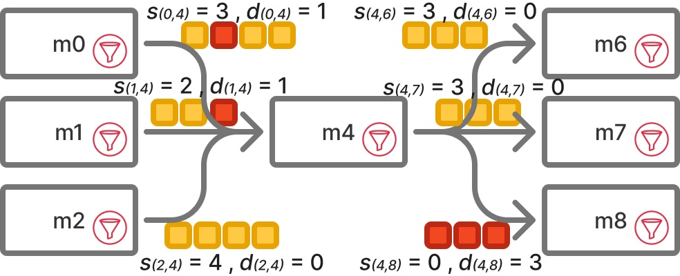
Figure 1 shows an example of \({s}_e\) and \({d}_e\) for the incoming and outgoing edges of a mix node \(m4\). For client-gateway links we assume \({d}_{(c,g)}=0\), since these are live bidirectional links where clients may retransmit packets until the gateway acknowledges reception. Thus, \({s}_{(c,g)}\) includes all the packets submitted under credential \(c\).6 At every subsequent hop, the quantities \({s}_e\) and \({d}_e\) of incoming and outgoing links of a gateway or node \(j\) satisfy the following relation: \[\sum_{i\in P(j)} {s}_{(i,j)} = \sum_{k\in S(j)} ({s}_{(j,k)} + {d}_{(j,k)}) \label{eq:sumpackets}\tag{1}\] where \(\sum_{i} {s}_{(i,j)}\) is the number of packets received by \(j\) from all its predecessors, \(\sum_{k} {s}_{(j,k)}\) is the number of packets successfully transmitted to successors, and \(\sum_{k} {d}_{(j,k)}\) is the number of packets received by \(j\) but dropped before reaching their next destination. In the example of Fig. 1: \(\sum_{i} {s}_{(i,4)}=9\), \(\sum_{k} {s}_{(4,k)}=6\), \(\sum_{k} {d}_{(4,k)}=3\).
Definition 1. A mixnet with reliability estimation (REst-mixnet) is a mixnet scheme over a graph \(G\) such that: (1) a publicly known number of legitimate packets \(\sum_c{s}_{(c,g)}\) are submitted via each gateway \(g\) during a time epoch; and (2) for any adversary \(\mathcal{A}\) conforming to the threat model in Section 2.2, all participants can estimate the reliability* \({\rho}_e\) of a link \(e=(i,j)\) in \(G\), defined as the fraction of legitimate packets successfully transmitted from \(i\) to \(j\), relative to the total legitimate packets received by \(i\) to be forwarded to \(j\), i.e.: \[{\rho}_e = \frac{{s}_e}{{s}_e + {d}_e}\]*
Anyone with access to the broadcast channel can compute a pair \((\hat{\rho}_e, \epsilon_e)\) such that \(|\hat{\rho}_e - \rho_e| \leq \epsilon_e\) holds with high confidence.
We additionally require the following two security properties.
Each legitimate packet must be processed at most once by any mix node. This is a standard property of decryption mixnets [13], [22], where packets leave a fingerprint at each hop that can be recognized in case of replay. Duplicate packets are thus detected and dropped by the receiving node.
The primary goal of a mixnet is to provide unlinkability between input and output packets, assuming an adversary that knows the sender and receiver sets, observes traffic in all the network links (including between clients and gateways) and even controls some of the participants. The reliability estimation mechanism must not leak any additional information that could help deanonymize packets.
3 Reliability Estimation Protocols↩︎
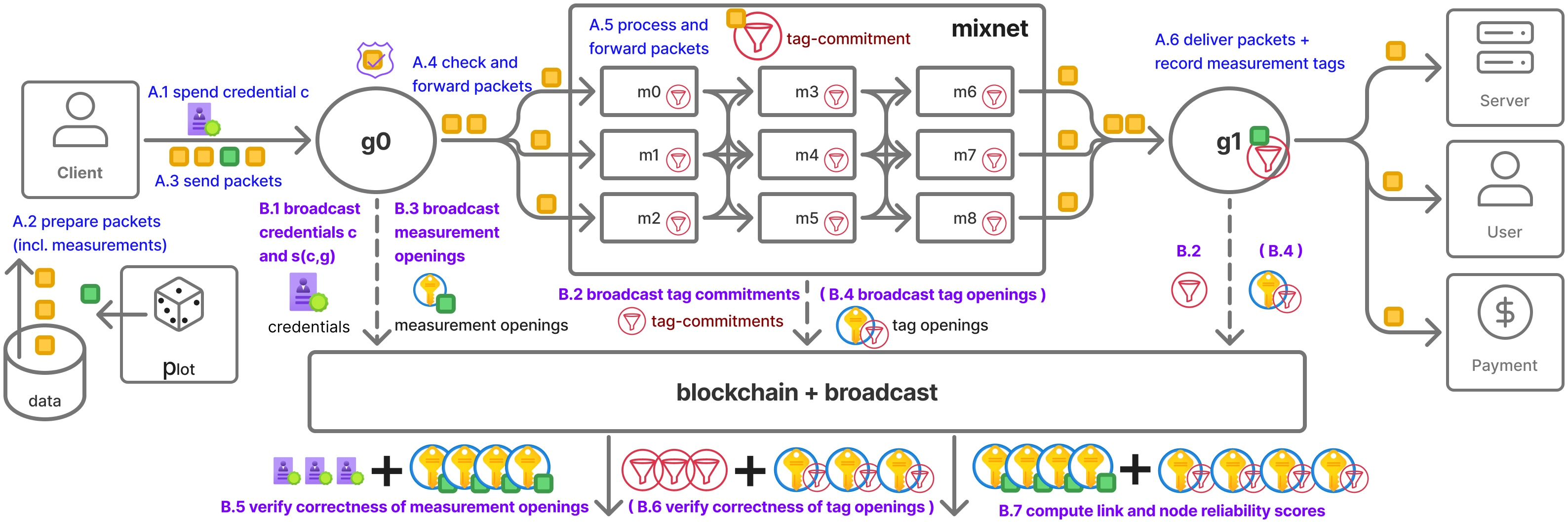
The core concept behind the system design is as follows: as illustrated in Fig. 2, our reliability estimation scheme relies on users with valid credentials sending indistinguishable measurement packets through the mixnet, interleaved with their normal client traffic (steps A.1-6). The key idea is to have gateways and mix nodes commit to the public key of credentials and packets (via unique tags) they have received (steps B.1-2) at the end of an epoch. These commitments to public keys, along with the measurement packets, are then opened (steps B.3-4) so that the measurements can be verified and traced along their paths through the mixnet (steps B.5-7). This process yields a sample of transmitted and dropped packets on each link, allowing anyone to estimate link and node reliability as we describe in the upcoming sections.
To summarize the protocols: Section 3.1 describes how users generate measurement traffic and how mix nodes record received packets in a semi-honest setting. A link reliability estimation protocol, which can be executed by anyone able to read the broadcast channel, aggregates the data broadcast by gateways and mix nodes to estimate the fraction of successfully transmitted packets on each network link, along with an associated error bound for a given confidence level. Section 3.2 then introduces VRF-based routing — a cryptographic tool that generates unforgeable measurement packets according to the mixnet’s routing policy and mitigates attacks by malicious clients and utility-maximizing gateways. Finally, Section 3.3 shows how link-level measurements can be used to derive reliability scores for mix nodes themselves.
3.1 Link Reliability Estimation in a Semi-Honest Setting↩︎
We begin by describing our link reliability estimation protocol in a simplified setting where clients and gateways are (semi-)honest. The steps are illustrated in Fig. 2.
Generation of packets. A client first spends (A.1) a credential \(c\) with a gateway \(g_0\), which entitles the client to route up to \(S_c\) packets through the mixnet via \(g_0\). Once the gateway acknowledges the credential, the client may submit packets. Each time a packet is created (A.2), a coin is flipped, and with probability \(p_\mathsf{lot}\) the packet header is used to generate a measurement (green packet) (A.3) that is sent interleaved with the client’s data and any added cover traffic (yellow packets). As routing intermediaries, mix nodes cannot distinguish measurement packets from other types; only the intended recipient can determine a packet’s type.
Let \({s}_{(c,g)} \leq S_c\) denote the total number of packets generated from credential \(c\) and routed via \(g\) during the epoch. Note that \({s}_{(c,g)} = S_c\) when a credential’s entire allowance is consumed within an epoch, which will often be the case for small \(S_c\). Importantly, each credential \(c\) is unlinkable to any other credential from the same wallet, preventing long-term profiling of client’s activities. The number of measurement packets \({s}_{(c,g)}^*\) follows a binomial distribution \({s}_{(c,g)}^{*} \sim B({s}_{(c,g)}, p_\mathsf{lot})\), and we expect \({s}_{(c,g)}^{*} \approx p_\mathsf{lot} \cdot {s}_{(c,g)}\). Measurement packets are sent interleaved with the client’s other traffic, while the commitments to measurement packets are retained by \(g\) (potentially also by the client) for later disclosure (in B.3). Routing of packets. Gateways forward client packets to the first-layer mix node specified in the packet’s route (A.4). Mix nodes then iteratively execute the packet processing algorithm and relay packets to their next hop (A.5). As part of replay protection, mix nodes must record a tag for each processed packet (denoted \(t\), cf. Sect. 3.2), e.g., computed as a hash of a secret derived via Diffie-Hellman by combining the packet header and the node’s private key. Upon receiving a packet, the node checks whether its tag is already in the list of seen tags: if the tag is new, the packet is processed and its tag added to the list; otherwise, the packet is dropped. Each node \(j\) stores, in a space-efficient manner, the \(\sum_i {s}_{(i,j)}\) tags received from its predecessors \(i \in P(j)\) during the epoch. This tag-commitment can be implemented via a Merkle tree [23] or a Bloom filter [24], as it only needs to be binding and space-efficient. We represent the nodes’ tag-commitments as the red filters in Fig. 2. When adding a fresh packet tag, the node appends to it a binary flag indicating whether the packet passed integrity checks. If so, it is relayed further; otherwise, it is dropped. Mix node decryption keys may be updated per epoch to provide forward security and prevent replay attacks across epochs. Measurement packets are addressed to a randomly selected gateway, with selection probabilities defined by the mixnet’s routing policy. Upon receiving a measurement packet, the gateway stores its tag in the tag-commitment and discards the (green) packet, while forwarding on data (yellow) packets as well as cover traffic to their respective destinations (A.6).
Post-epoch stage: revelation of measurements. Once an epoch concludes, the protocol proceeds with the broadcasting steps shown in Fig. 2:
B.1: Each gateway \(g\) broadcasts the number of packets \({s}_{(c,g)} \leq S_c\) sent per credential \(c\) during the epoch.
B.2: All nodes (mix nodes and gateways) broadcast their tag-commitments.
B.3: Each gateway \(g\) broadcasts the openings of the \({s}^*_{(c,g)} (\approx p_\mathsf{lot} \cdot {s}_{(c,g)})\) measurement packets generated during the epoch from all its client credentials.
B.4: All mix nodes and gateways broadcast the openings of their tag-commitments corresponding to the revealed measurement packets (this step is unnecessary if Bloom filters are used, since membership can be verified directly). Note only public material is broadcast, not secret key material.
Any party observing the broadcasts can verify correctness and compute a reliability score \(\hat{\rho}_e\) per link \(e\):
B.5: Reconstruct the \(\sum_g \sum_c {s}^*_{(c,g)}\) measurement packets generated during the epoch (including their mixnet paths, recipient gateways and per-hop tags) using the gateway openings.
B.6: Verify the validity of the measurement tag openings provided by mix nodes and gateways.
B.7: Determine which measurement packet tags are present in which tag-commitments, yielding the sets of transmitted \({s}^*_{e}\) and dropped \({d}^*_{e}\) measurement packets for each link \(e\). Link and node reliability scores can be then derived from \({s}^*_{e}\) and \({d}^*_{e}\), as explained in the following.
Given a link \(e=(i,j)\), we denote by \({s}_{(i,j)}^*\) the amount of measurement packets successfully transmitted in the link (number of measurement packets whose (per-hop) tags appear in the tag-commitments of both \(i\) and \(j\)), and by \({d}_{(i,j)}^*\) the number of measurement packets dropped in the link, i.e., those whose tags appear in the tag-commitment of \(i\) but not the one of \(j\). Similarly to Eq.@eq:eq:sumpackets , for any node \(j\), all the measurement packets received from its predecessors \(i\) are either successfully transmitted to their next destination \(k\), or dropped before reaching \(k\):
\[\sum_i {s}^*_{(i,j)} = \sum_k ({s}^*_{(j,k)} + {d}^*_{(j,k)}) \label{eq:node-samples}\tag{2}\]
Measurement packets revealed by a gateway \(g\) and addressed to first-layer node \(i\) that do not appear in \(i\)’s tag-commitment are considered as part of \({d}^*_{(g,i)}\). Similarly, \({d}^*_{(k,g)}\) accounts for measurement packets addressed to \(g\) from last layer node \(k\) that are reported by \(k\) but do not appear in \(g\)’s tag-commitment. Packets reported as dropped due to failed integrity checks (as indicated by the binary flag stored with each tag) are excluded from the measurement sample. Likewise, packets whose paths exhibit ‘holes’ — i.e., those included in a node \(j\)’s tag-commitment but missing from a predecessor’s — are also discarded as measurements.
Since mix nodes cannot distinguish measurement packets from regular ones, measurement traffic experiences the same drop behavior as user traffic. We use this to produce a reliability score \(\hat{\rho}_e\) per link \(e\), given by the transmitted and dropped samples \({s}_e^*\) and \({d}_e^*\), defined as:
\[\label{eq:rho95e95hat} \hat{\rho}_e = \frac{{s}_e^*}{{s}_e^* + {d}_e^*}\tag{3}\]
The accuracy of \(\hat{\rho}_e\) as an estimator of \({\rho}_e\) depends on the available number of measurement samples \({s}_e^* + {d}_e^*\), which determine the maximum sampling error \(\epsilon_e\) with a given a confidence level, such that:
\[\label{eq:estimation} |{\rho}_e - \hat{\rho}_e| \leq \epsilon_e\tag{4}\]
To bound the estimation error \(\epsilon_e\) we use methods that estimate coin bias from a sequence of observed coin flips, considering that the coin flip can result in transmission (heads) with probability \({\rho}_e\); or in a drop (tails) with probability \(1-{\rho}_e\). Without having any prior for the distribution \({\rho}_e\), i.e., assuming all values are equally likely, \({\rho}_e\) follows a Beta distribution with density function \({\rho}_e^{s^*_e} (1- {\rho}_e)^{d^*_e} / B( s^*_e +1, d^*_e+1)\), mean \(\hat{\rho}_e\) and variance \(\hat{\rho}_e \cdot (1-\hat{\rho}_e) / (s^*_e + d^*_e + 1)\).
When the number of samples is sufficiently large and the coin bias is not heavily skewed, we can apply a normal approximation7 that yields the Wald interval for the maximum estimation error \(\epsilon_e\) at confidence level \(Z\):
\[\label{eq:epsilon} \epsilon_e = Z \cdot \sqrt{\frac{\hat{\rho}_e \cdot (1 - \hat{\rho}_e)}{{s}_e^* + {d}_e^*}}\tag{5}\]
Note that the estimation accuracy for an edge \(e\) depends only on the total number of measurement packets successfully collected on it, i.e., \({s}_e^* + {d}_e^*\). This implies that the error bound \(\epsilon_e\) is independent of the total volume of user traffic (\({s}_e + {d}_e\)) or the packet size. As a result, the protocol remains efficient and scalable even as the overall traffic grows. In particular, to achieve a target error \(\epsilon\), it suffices to maintain a constant number of measurements per link, regardless of how much total traffic the link handles. Consequently, as traffic increases, the measurement sampling rate \(p_\mathsf{lot}\) can be decreased while still maintaining estimation accuracy. Conversely, a sudden drop in traffic volume may yield too few measurement samples, leading to less accurate reliability estimates for that epoch; however, \(p_\mathsf{lot}\) can be adjusted dynamically each epoch based on observed traffic to ensure sufficient samples for the desired accuracy. The output of this protocol is a value \(\hat{\rho}_e \approx {\rho}_e\) for each edge e, estimating the link reliability (i.e., the fraction of successfully transmitted packets), along with a sampling error \(\epsilon_e\) that quantifies the estimate’s accuracy at a given confidence level.
There are various options for implementing tag-commitments, including Merkle trees [23] and Bloom filters [24]. Broadly speaking, the relevant cryptographic primitive is that of a vector-commitment [26]. In the remaining of the paper we focus on the case of Merkle Tree based vector commitments. Beyond avoiding false positives, Merkle Trees prevent a membership-test attack feasible with Bloom filters: a client whose keys are compromised could otherwise have past packet routes reconstructed from the published filters. Moreover, Merkle Trees scale better at high traffic volume and low \(p_\mathsf{lot}\).
For \(n\) measurement packets, the overhead consists of transmitting these \(n\) packets through the mixnet and performing \(O(n \log n)\) broadcasts when Merkle trees are used for tag-commitments. In Appendix 10 we estimate the overhead incurred in a practical deployment.
The scheme does not reveal any information about clients’ packet routes or destinations, given that revealed measurement packets contain no client payloads and are addressed to random destinations. Only the total number of packets generated per credential is required, and this information is already observable by a network adversary monitoring the connection between a client and its gateway. Credentials are unlinkable to each other, disaggregating clients’ activities over time. Note the tradeoff between credential size (in terms of number of packets \(S_c\)) and privacy: a smaller \(S_c\) provides finer-grained disaggregation of usage per client but incurs greater overhead for credential issuance and verification, as more credentials must be handled for the same packet volume. Ideally, credentials should have a size \(S_c\) that is typically consumed within a single epoch.
3.2 VRF-Based Routing for Link Reliability Estimation in an Adversarial Setting↩︎
We now extend the link reliability estimation protocol to an adversarial setting, where clients may be malicious and gateways act as utility-maximizing entities. A utility-maximizing gateway avoids strategies that would decrease its utility, but may otherwise deviate arbitrarily from the protocol. We assume a gateway utility function8 that increases monotonically with the following factors: (i) link reliability, as estimated by the protocol, for mixnet links involving the gateway; (ii) client satisfaction, defined as the fraction of a client’s submitted packets that are successfully delivered; (iii) credential consumption, i.e., the number of announced legitimate packets sent; and (iv) adherence to protocol specifications, such that the gateway is not caught misbehaving.
Viewed in this utility-maximizing setting, the scheme of the previous section is insufficient. For instance, a utility-maximizing gateway could send and open specially crafted packets that partially match the sent measurements. This can be done in such a way so that it preserves the gateway’s perceived reliability on its own links (thus maintaining its own utility), while degrading the perceived reliability of downstream links, as it appears that those measurements got dropped along their path by downstream nodes. Also, since clients can be malicious in our model (as e.g., in a setting where a utility-maximizing gateway employs some clients as sock puppets), we cannot rely on them to generate the measurement traffic, as they may, e.g., manipulate measurement traffic to reduce the reputation of otherwise reliable nodes. To ameliorate these issues and demonstrate how we can still measure link reliability in this setting we put forward a method that ensures that path selection cannot be biased:
VRF-based routing. At a high level, VRF-based routing eliminates any client or gateway control over the random values that determine packet routing parameters. Clients can only choose the payloads and final destinations for non-measurement packets. Everything else, including the randomness used for encryption, is derived deterministically and verifiably from publicly known values. This enforces non-manipulable path selection and, specifically in our setting, guarantees that measurement packets cannot be forged, omitted, or selectively dropped without detection. In more detail, our construction relies on:
(1) A VRF function that consists of three algorithms \(\langle \mathsf{K}, \mathsf{E}, \mathsf{V}\rangle\): \(\mathsf{K}\) generates a key pair \((sk,vk)\); \(\mathsf{E}(sk, m) = (r, \pi)\) evaluates the VRF on \(m\) to produce the pseudorandom output \(r\in\{0,1\}^\kappa\) as well as a proof \(\pi\); and \(\mathsf{V}(vk, m, r, \pi)\) verifies that \(r\) is the correct output corresponding to the message \(m\).
(2) A mixnet packet encoding scheme (e.g., Sphinx [16]) that sets the individual hops in a packet’s path and enables its processing.
(3) Non-interactive zero-knowledge proofs for discrete logarithm relations, for which we use standard notation, e.g., \(\mathsf{NIZK}( ( g,y )\,\exists x :g^x = y)\) denotes a proof where the statement is a concise description of a multiplicative group generated by \(g\) as well as an element \(y\) in that group and the witness is the discrete logarithm of \(y\) base \(g\).
(4) A public algorithm \(\mathsf{Routing}(i, r) = j\) that for a given mixnet node \(i\) and randomness \(r\), samples the node that should be the next hop \(j\), assuming \(r\) is uniformly distributed over \(\{0,1\}^\kappa\). A common choice for \(\mathsf{Routing}\) is to sample uniformly at random from the successor nodes \(j \in S(i)\) in the graph \(G\). We will further require that for any \((i,j)\), the distribution of \(r\) conditioned on \(\mathsf{Routing}(i, r) = j\) is efficiently samplable.
(5) A public broadcast channel, like a blockchain, that also facilitates a beacon in the form of a random nonce \(\mathsf{n}\) (this value can be derived by the blockchain itself cf. [27]).
We describe the concept of VRF-based routing in terms of encoding and processing packets. An overview of the notations used in the description is presented in Table ¿tbl:tab:notation?.
\(\kappa\): security parameter; length of the hash function output \(p_\mathsf{lot}\): probability of a measurement packet \(ctr\): packet counter used as VRF input \(L\): number of layers in the mixnet \(W\): width of the mixnet \(N=LW\): number of mixnodes \(i,j,k,\ldots\): nodes in the network graph \(S_c\): number of packets enabled by credential \(c\) \(\rho\): reliability coefficient \(\hat\rho\): estimation of reliability coefficient \(e=(i,j)\): link (edge) of network graph between nodes \(i,j\) \(s_e\): number of successfully transmitted legitimate packets along network link \(e\) \(d_e\): number of dropped legitimate packets along network link \(e\) \(s^*_e\): number of measurement packets successfully transmitted along network link \(e\) \(d^*_e\): number of measurement packets dropped along network link \(e\) \(vk\) : verification key of the VRF \(sk\) : secret key of the VRF \(r_\mathsf{type}\): VRF value for measurement lottery \(r_\mathsf{pkt}\): VRF value for packet encoding \(r_\mathsf{exit}\): VRF value for choosing the exit gateway \(y_{n}\): public-key of node \(n\) \(T\): target that determines measurement lottery outcome \(s_i\): Diffie Hellman key corresponding to packet hop \(i\) \(b_i\): blinding value corresponding to packet hop \(i\) \(\tilde{r}_i\): encoding randomness for packet hop \(i\) \(n_i\): node corresponding to packet hop \(i\) \(\mathsf{n}\): unpredictable nonce drawn used as VRF input \(\alpha\): client chosen packet randomization key \(\alpha_0\): packet specific randomization key \(\alpha_i\): base element for \(i\)-th packet hop, for \(i>0\) \(\psi_i\): ciphertext for packet hop \(i\) \(x_i\): secret-key of processing node in packet hop \(i\) \(t_i\): pseudorandom tag calculated in packet hop \(i\) |
|---|
Packet encoding. Packet encoding involves a client with credential \(c\) and its entry gateway \(g_0\). For a given \(c\), the client selects a packet randomization key \((\alpha = g^{x},x)\) and the gateway a VRF key pair \((vk, sk)\). These values are publicly committed on the public broadcast channel. Furthermore, both client and gateway maintain a packet counter. For each packet transmission of a data packet or measurement packet by the client, three VRF outputs are computed, \(r_\mathsf{pkt} , r_\mathsf{type} , r_\mathsf{exit}\) each taking as input the packet counter and a public random nonce \(\mathsf{n}\) that must be unpredictable at the time when public keys are committed. The key idea is to use the VRF to “derandomize” the mixnet encoding ensuring two properties simultaneously. First, based on the VRF output, with probability \(p_\mathsf{lot}\) the packet encoding is fully determined by the VRF and corresponds to a measurement packet (\(p_\mathsf{lot}\) is the probability of the event \(r_\mathsf{type}<T\), where \(T\) is a suitable public target value). This ensures that measurement packets are fully reproducible by the gateway \(g_0\), who is able to open measurement tag-commitments on behalf of the client—thus removing the need for clients to be online and participate in the post-epoch steps of the protocol. This exploits the fact that once selection is unbiasable, who generates the measurements becomes a practical choice. Having the gateway hold and submit the measurement openings post-epoch is more practical, since gateways are typically online while clients (e.g., on mobile devices) may have intermittent connectivity. Second, non-measurement packet headers are deterministically computed based on both the VRF and the packet randomization key \(\alpha\), so that, in the view of the gateways they remain computationally indistinguishable from regular packets under the underlying encoding scheme, hiding both their payload as well as the mixnet path they follow.
To achieve these two properties, each packet involves the calculation of a sequence of randomizer values \(\alpha_0, \alpha_1, \ldots\), one for each hop in the packet route, where \(\alpha_0 = g^{r_\mathsf{pkt}}\) or \(\alpha_0 = \alpha^{r_\mathsf{pkt}}\) depending on whether it is a measurement or non-measurement packet. The remaining values in the sequence are derived by repeatedly blinding \(\alpha_0\) with pseudorandom exponents, as detailed below. This sequence of values \(\alpha_0, \alpha_1, \ldots\) is used to generate ephemeral Diffie–Hellman secrets with the public key of each node in the path, starting from the gateway \(g_0\). This secret, denoted by \(s_i\) at hop \(i\), is deterministically derived from the VRF output and the randomization key \(\alpha\), but appears pseudorandom to any third party. These secrets are used to derive the blinding exponent for the next element in the randomizer sequence as well as to seed the mixnet encoding. Moreover, most importantly, they also determine the next hop in the routing sequence by applying the \(\mathsf{Routing}(\cdot ,\cdot )\) function to the identity of the current node and a pseudorandom value derived by the key itself (see Fig. 3 and Table ¿tbl:tab:notation?).
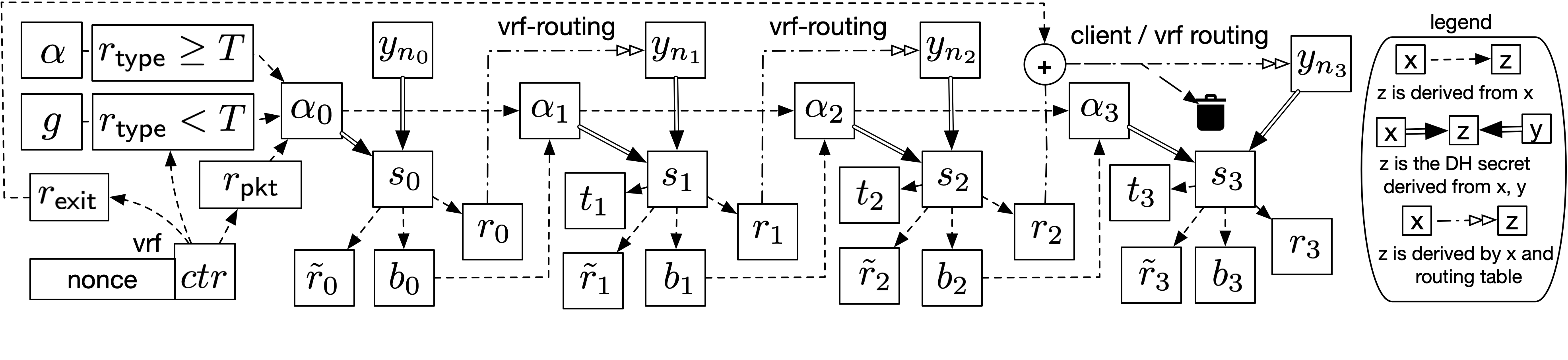
A final subtlety arises when selecting the exit gateway \(g_1\). For non-measurement packets, this gateway should be chosen at the discretion of the client; for measurement packets, it is pseudorandomly determined by the VRF.9 To prevent the final mix node from detecting which case applies, a value \(\tilde{r}_\mathsf{exit}\) is embedded in the payload available to the last hop and xor-ed into the randomness used in the \(\mathsf{Routing}\) calculation. For measurement packets, \(\tilde{r}_\mathsf{exit}\) is generated by the VRF, while for non-measurement packets is selected so that the output of \(\mathsf{Routing}(\cdot ,\cdot )\) matches the desired exit gateway.
In more details, suppose the client has selected an entry gateway \(n_0\) with key \(y_0\) and an exit gateway \(n_\nu\), where \(\nu>0\) is the number of packet hops. Recall, the gateway has already established a VRF key \((vk, sk)\), and the client a (packet) randomization key \((\alpha = g^{x}, x)\). The gateway computes three VRF values \(r_\mathrm{pkt} = \mathsf{E}(sk, \mathsf{n} || ctr || \mathsf{pkt})\), \(r_\mathrm{exit} = \mathsf{E}(sk, \mathsf{n} || ctr || \mathsf{exit})\), \(r_\mathsf{type} = \mathsf{E}(sk, \mathsf{n} || ctr || \mathsf{type})\), where \(\mathsf{pkt}, \mathsf{type}, \mathsf{exit}\) are the numerical labels \(\{0,1,2\}\); note we use \(||\) to denote concatenation. In case \(r_\mathsf{type} < T\), then the packet associated with \(ctr\) is a measurement packet, otherwise we have a regular packet. In the latter case, the client receives the VRF values from the gateway, and calculates \(\alpha_{0} = \alpha^{r_\mathsf{pkt}}\), \(s_0 = y_0^{r_\mathsf{pkt} \cdot x}\), \(\tilde{r}_0 = H(\mathsf{rnd}, s_0)\), \(r_0 = H(\mathsf{next}, s_0)\), \(b_0 = H(\mathsf{bli},s_0)\), where \(\mathsf{rnd}, \mathsf{next}, \mathsf{bli}\) are the numerical labels \(\{3,4,5\}\) respectively. Subsequently (for \(i=1,\ldots,\nu\)), \(\alpha_i = \alpha_{i-1}^{b_{i-1}}\), \(s_i = y_i^{r_\mathsf{pkt} \cdot x}\), where \(y_i\) is the key of node \(n_i = \mathsf{Routing}(n_{i-1}, r_{i-1})\) (for \(i<\nu\)), and finally, as before, \(\tilde{r}_i = H(\mathsf{rnd}, s_i)\), \(r_i = H(\mathsf{next}, s_i)\), \(b_i = H(\mathsf{bli},s_i)\). In the above, we have the exception in the calculation \(n_\nu\) so that \(n_\nu = \mathsf{Routing}(n_{\nu-1}, r_{\nu-1}\oplus \tilde{r}_\mathsf{exit})\), with \(y_\nu\) being the key of the exit gateway and \(\tilde{r}_\mathsf{exit}\) selected suitably so the routing to \(n_\nu\) holds (the value \(r_\mathsf{exit}\) is not used). In the case of a measurement packet, the procedure is the same with the distinction that \(x=1\) in the calculations provided above, i.e., the randomness key \(\alpha\) is not involved and as a result \(\alpha_0 = g^{r_\mathsf{pkt}}\) and the gateway can calculate the measurement packet directly. Moreover, the exit gateway is defined randomly by choosing \(\tilde{r}_\mathsf{exit} =r_\mathsf{exit}\). In either case, the above process enables to apply the mixnet encoding along the route \(\langle n_0, \ldots, n_{\nu-1}, n_\nu\rangle\), using randomness \(\tilde{r}_i\) at the \(i\)-th hop. The resulting packet is augmented with the value \(\alpha_0\). Note that the packet counter \(ctr\) is incremented with each packet.
Packet Processing. All the packets have the form \((\alpha_i, \psi_i)\), where \(\alpha_i\) is the randomizer value associated with the packet and \(\psi_i\) is the packet itself. Assuming the processing node has public-key \(y_i = g^{x_i}\), the first step is to compute \(s_i=\alpha^{x_i}\), a Diffie-Hellman secret used to process \(\psi_i\). Of particular importance is the tag value \(t_i\), derived from \(s_i\). This tag is stored in the tag-commitment along with a binary flag indicating whether all packet validation checks passed. Some additional care is needed when the processing node is the entry gateway \(g_0\) or the last node of the mixnet. In the former case, recall \(g_0\) controls the VRF key and can thus determine whether a packet is a measurement packet. In this case, the packet may be fully verified (its computation may even be delegated by the client to the gateway). For a non-measurement packet, observe that \(g_0\) can still verify that the \(\alpha_0\) value is correctly derived from the client’s randomization key \(\alpha\) and the VRF output \(r_\mathsf{pkt}\). When the last node of the mixnet processes the packet, it extracts the value \(\tilde{r}_\mathsf{exit}\) and uses it to compute the next hop via the \(\mathsf{Routing}()\) function.
In more details, the processing of a packet \((\alpha_0, \psi_0)\) corresponding to VRF values \(r_\mathsf{pkt}, r_\mathsf{type}, r_\mathsf{exit}\) proceeds as follows. The gateway calculates \(s_0 = \alpha_0^{x_0}, \tilde{r}_0 = H(\mathsf{rnd}, s_0)\), where \(x_0\) is its secret-key and it verifies that: (I) the mixnet encoding was correctly applied to produce \(\psi_0\) given randomness \(\tilde{r}_0\) and the public key \(y_0\); and (II) the per packet randomization key is correctly computed: in the case of a non-measurement packet it is \(\alpha_0 = \alpha^{r_\mathsf{pkt}}\), while it is \(\alpha_0 = g^{r_\mathsf{pkt}}\) in the case of a measurement packet. If these checks pass, it calculates the next hop as \(n_1 = \mathsf{Routing}(n_{0}, r_0)\), where \(r_0 = H(\mathsf{next}, s_0)\) and then it forwards \((\alpha_1, \psi_1)\) to node \(n_1\), where \(\alpha_1 = \alpha_0^{b_0}\) with \(b_0 = H(\mathsf{bli}, s_0)\) and \(\psi_1\) is the payload of packet \(\psi_0\) after processing it in the way the mixnet decoding requires.
Next we illustrate how processing works for the remaining nodes in the path. Node \(n_i\), given \((\alpha_i, \psi_i)\) for \(i=1,\ldots,\nu\), operates as follows. First, it processes the packet to reveal payload \(\psi_{i+1}\) and if \(i<\nu\), the next hop \(n_{i+1}\). Then it calculates \(s_i = \alpha_i^{x_i}\), \(\tilde{r}_i = H( \mathsf{rnd} , s_i)\), and if \(i<\nu\), \(\alpha_{i+1} = \alpha_i^{b_{i}}\) where \(b_{i} = H(\mathsf{bli}, s_i)\). The node then verifies that (I) the mixnet encoding was correctly applied to produce \(\psi_i\) given randomness \(\rho_i\), (II) in case \(i<\nu-1\), \(n_{i+1} = \mathsf{Routing}(n_{i}, r_{i})\) where \(r_{i} = H(\mathsf{next}, s_{i})\), (the randomized routing check). It also calculates the tag \(t_i = H(\mathsf{tag}, s_i)\), and stores \((b_i, \mathrm{flag}_i)\) in a database of processed tags where \(\mathrm{flag}_i\) is \(1\) if and only if the integrity check of \(\psi_i\) is valid. The case \(i=\nu -1\) is similar but also involves pulling \(\tilde{r}_\mathsf{exit}\) from the payload and calculating \(n_{\nu } = \mathsf{Routing} (n_{\nu-1} , r_{\nu-1} \oplus \tilde{r}_\mathsf{exit})\). In any case, when \(i<\nu\), the node forwards \((\alpha_{i+1}, \psi_{i+1})\) to node \(n_{i+1}\). Finally, in case \(i=\nu\), the payload \(\psi_{\nu+1}\) is parsed as the plaintext and is processed by node \(n_\nu\).
Recall the key point of the above construction is that the randomness used for encoding is pseudorandomly determined by the key \(\alpha\) and the VRF function. Specifically, for each \(ctr\), there is a per packet randomization key \(\alpha_0 = g^{x\cdot r_\mathsf{pkt}}\) that is used to seed the mixnet encoding. For measurement packets, the gateway can completely validate their computation since \(r_\mathsf{pkt}\) is known to it and the secret randomization key \(x\) of the client is not used in the packet calculations. The same holds true for any party that obtains the value \(r_\mathsf{pkt}\). Furthermore, any packet can be demonstrated to be a measurement or not, by checking the inequality \(r_\mathsf{type}<T\) which is true iff the \(ctr\) value corresponds to a measurement packet.
The following theorem is a straightforward consequence of the above observations. The first and third statements follow from the Diffie Hellman assumption and the security of the VRF, the fourth relies on the VRF, while the second takes advantage of the random oracle modeling the hash function and the fact that routing choices depend on the unpredictable value of a nonce \(\mathsf{n}\). A proof is provided in Appendix 7.
Theorem 1. Assuming the pseudorandomness of the VRF, the Decisional Diffie Hellman assumption, the hash functions are modeled as random oracles and the underlying encoding satisfies security and privacy, it holds that: (I) given a packet \(\langle \alpha, \psi\rangle\) which is routed to an honest node so that it encodes one of two payloads \(M_0, M_1\), it is infeasible for the adversary to guess which payload it contains with probability better than random — this is true even in the setting \(vk\) is adversarially chosen; (II) given two packets \(\langle \alpha_0, \psi_0\rangle\) and \(\langle \alpha_1, \psi_1\rangle\) that when routed to an honest node result to the processed packets \(\langle \alpha^*_0, \psi^*_0\rangle\) and \(\langle \alpha^*_1, \psi^*_1\rangle\), it is infeasible for the adversary to guess \(b\) with probability better than random, given \(( \langle \alpha_{b}^*, \psi_{b}^*\rangle, \langle \alpha_{1-b}^*, \psi_{1-b}^*\rangle\) — this is true even in the setting \(vk\) is adversarially chosen; (III) the packet routes generated by the above process are sampled according to \(\mathsf{Routing}()\) pseudorandomly, even in the setting where \(vk, \alpha\) are adversarially chosen; (IV) measurement packets are computationally indistinguishable from non-measurement packets in the perspective of any mix node.
We now revisit the construction of Section 3.1 and augment it with VRF-based routing. We highlight only the changes.
Cryptographic primitives. The VRF function can based on Dodis Yampolskiy’s PRF [28]; specifically, \(\mathsf{K}\) produces a secret key \(sk_\mathsf{vrf}\) and public-key \(vk_\mathsf{vrf} = g^{sk_\mathsf{vrf}}\), while the VRF evaluation is set to \(\mathsf{E}(\mathsf{n}|| ctr || \mathrm{label} ) = (r_\mathsf{label} , \pi)\) where \(r_\mathsf{label} = H(vk_\mathsf{vrf}, g, u_\mathrm{label})\), \(u_\mathrm{label} = g^{1/(sk_\mathsf{vrf} + 2^\ell \mathsf{n} + 4 \cdot ctr + \mathrm{label} + 1 )}\), and \(\pi_\mathrm{label} = (u_\mathrm{label}, \pi'_\mathrm{label})\) with \(\pi'_\mathrm{label} = \mathrm{NIZK}( g, vk_\mathsf{vrf}, u_\mathrm{label}, ctr, \ell, \mathsf{n}, \mathrm{label}: \exists sk_\mathsf{vrf}( u_\mathrm{label}^{sk_\mathsf{vrf}+2^\ell \mathsf{n} + 4 ctr + \mathrm{label}+1})\) \(|| vk\) : verification key of the VRF \(g \land vk_\mathsf{vrf} = g^{sk_\mathsf{vrf}}))\). Note in the above \(\ell, \mathrm{label}\in\mathbb{N},\) are public values and \(ctr< 2^{\ell-2}\) always where \(ctr\) is the packet counter.
Generation of packets. Step A.1 is augmented to include the setup of the public values \(\alpha\) and VRF key \(vk\). Together with the acknowledgment of credential, the gateway shares the VRF secret-key \(sk\) with the client. Subsequently, step A.2 follows the packet encoding process of VRF-based routing, with probability \(p_\mathsf{lot}\) determined by threshold \(T\). In addition to measurement and regular non-measurement packets, we assume the client also sends special non-measurement packets called self-loops.
Self-loops. A self-loop is a packet that a client sends to itself via the mixnet. In prior work [13] and in the deployed Nym mixnet,10 self-loops are a type of cover traffic that enhances privacy by providing unobservability properties. In our context, self-loops additionally enable a client to monitor the reliability of the entry gateway it has selected, by checking whether packets are successfully delivered (the gateway cannot distinguish such cover traffic from data packets received for that client). A client can switch to a different gateway (with a new credential) if it finds the current gateway’s reliability unsatisfactory.
Steps A.3 and A.4 remain unaltered, with the only difference being that packet integrity checks are enhanced by incorporating how the VRF is used to compute the randomizer values. Steps A.5, as well as B.1-B.2, remain unchanged. Step B.3, however, is modified to reflect the use of VRFs in generating measurement packets:
Opening a measurement packet. Opening a measurement packet corresponding to a credential containing \(\alpha\) is done by revealing the values \((ctr, r_\mathsf{pkt}, \pi_\mathsf{pkt}, r_\mathsf{type}, \pi_\mathsf{type} , r_\mathsf{exit}, \pi_\mathsf{exit})\). In this case, anyone can verify in step B.5 that the packet is a measurement packet corresponding to counter \(ctr\) by checking that \(r_\mathsf{type}<T\) and validating the proofs. Moreover, the full computation of the packet is verifiable, as the packet can be deterministically regenerated from the values \(r_\mathsf{pkt}\) and \(r_\mathsf{exit}\), together with the packet counter \(ctr\) and the public nonce \(\mathsf{n}\). As for the size of the opening, it requires one counter value, one group element, one hash, and two exponents, for each of the three VRF openings. Instantiating the base group via Ed25519, results in \(388\) bytes per measurement opening.
Proof of no-skipping. In addition to the above, at step B.3, the gateway must demonstrate that it sent all measurement packets. Specifically, for any counter value \(ctr\) that does not correspond to a measurement packet, the gateway can open the VRF value corresponding to this counter in the packet sequence and demonstrate that it corresponds to a non-measurement legitimate packet. Namely, the gateway reveals the tuple \(\langle ctr, r_\mathsf{type}, \pi_\mathsf{type} \rangle\), which can be verified against \(vk\) using the test \(r_\mathsf{type}\geq T\). Given that all measurement packets have been opened, a random subset of the complement set of non-measurement counters can be challenged in this way to ensure that no measurement packets have been skipped. The randomness can be derived from a public nonce that is drawn after steps B.1 and B.2 have completed. In more detail, suppose we want to ensure that the amount of skipping is below a certain threshold, say, \(\tau_\mathsf{s}\). Then by testing \(v\) random non-measurement packets, if the skipping rate is at least \(\tau_\mathsf{s}\), we will fail to detect it with probability \((1-\tau_\mathsf{s})^v\). It follows that we can set \(v = \log(1/\epsilon)/\log(1-\tau_\mathsf{s})^{-1}\), where \(\epsilon\) is the desired error probability. In terms of size of a single opening, we must reveal one index, one group element, one hash, and two exponents for the proof. Using Ed25519, this amounts to 132 Bytes per counter position.
We next illustrate how these adjustments to the link estimation protocol of Section 3.1 mitigate all attacks in our threat model.
The protocol augmented with VRF-based routing is also extended by having gateways broadcast proofs of no-skipping (as a second part of step B.3 in Fig. 2), ensuring that (almost) all measurement packets are accounted for. The first key observation is that, conditional on a legitimate packet being sent by a gateway, we obtain a coin flip with probability \(p_\mathsf{lot}\) for sending a measurement packet. Due to gateways being utility-maximizers, observe that the total number of announced packets sent by gateway \(g\), \(S_g = \sum_{c} s_{(c,g)}\), is at least as large as the actual number of packets sent.
We next require that entry gateways open all the measurement packets in the announced ranges for each credential. Due to the proof of no skipping, any gateway that does not want to get caught lying must open all the measurement packets in the range for each credential it announced. Moreover, note that if there is a credential that is misreported to have been used less than in reality, e.g., the declared \(s_{(c,g)}\) is smaller than the actual \(s^\mathsf{a}_{(c,g)}\), then there must exist another credential \(c'\) reported by the same gateway that compensates for it, i.e., such that \(s^\mathsf{a}_{(c',g)}<s_{(c',g)}\). It follows that for credential \(c'\) there are measurement packets that have not been opened — thus exposing gateway \(g\), who will be caught in the proof of no-skipping for credential \(c'\). Furthermore: (1) If measurement packets are not sent (despite being opened), this will reduce the measured reliability of the gateway, so a utility-maximizing gateway will not perform this action. (2) If non-measurement legitimate packets are selectively not sent (despite having the opportunity to send them) there are two possibilities: (i) the non-measurement packets are simply dropped, in which case client satisfaction decreases and thus the gateway will not prefer this strategy; (ii) a gateway that colludes with the client may substitute legitimate packets by illegitimate packets that carry the same payload — this does not affect our estimation, which is only concerned with the reliability of legitimate packets.
For receiving gateways, assuming they are utility-maximizers, we observe: (1) If measurement packet tags are not recorded by the gateway in the tag-commitment despite being received, the measured reliability will drop, hence the gateway will not perform this action. (2) If non-measurement packets are not handed over to their destination this means that they have been processed, identified as non-measurement and then dropped. This affects client satisfaction (clients do not receive response traffic and are likely to switch to another gateway), and as a result, is not a preferred strategy of a utility-maximizer gateway. In summary, with VRF-based routing, there is no strategy available to a utility-maximizing gateway (or malicious client) that can bias link reliability estimation in the mixnet.
3.3 Node reliability estimation↩︎
The described reliability estimation protocol provides per-link reliability estimates. However, what is needed for effective network management, e.g., to determine which nodes to include in the mixnet, is a per-node reliability score. Each link involves two nodes: a predecessor who sends packets and a successor who receives them, so estimating node reliability entails distributing responsibility for observed packet drops between the two endpoints of a faulty link. In this section, we show how to derive node reliability scores from the set of successful and failed link measurements \({s}^*_e\) and \({d}^*_e\).
The goal of this protocol is to estimate, for every node \(j\) participating in the mixnet,11 a reliability score \(\hat{\rho}_j\) that reflects the rate of packet losses attributable to \(j\), where \(\hat{\rho}_j=0\) means that \(j\) dropped all packets sent to it (e.g., if \(j\) is offline for the entire epoch) and \(\hat{\rho}_j=1\) indicates that the node was consistently online and correctly processed and forwarded all received packets. These \(\hat{\rho}_j\) can be computed by any entity that knows the outputs of the protocol described in Sect. 3.1; that is, the counts \({s}^*_e\) and \({d}^*_e\) of successfully transmitted and dropped measurement packets per link \(e \in G\). We consider reliable inter-node transmissions such that any packet drops are either due to a failure of the link predecessor or the successor. The estimated node reliability \(\hat{\rho}_j\) is computed as:
\[\hat{\rho}_j = \frac{\sum_{k \in S(j)} ({s}^*_{(j,k)} + \hat{\beta}_{(j,k)} {d}^*_{(j,k)})}{\sum_{i \in P(j)} ({s}^*_{(i,j)} + \hat{\beta}_{(i,j)} {d}^*_{(i,j)})} \label{eq:estimated95node95perf}\tag{6}\]
In the case of gateways, \(\hat{\rho}_g\) is computed considering the successfully transmitted (and dropped) measurements to first-layer node successors \(k \in S(g)\) (\(g\)’s outgoing links), and the received (and dropped) measurements from last-layer node predecessors \(i \in P(g)\) as recorded in their tag-commitment (\(g\)’s incoming links).
The parameter \(\hat{\beta}_{e}\) denotes the fraction of drops attributed to the link successor, with the remaining \(1-\hat{\beta}_{e}\) being attributed to the link predecessor. Ideally, participants verify that \(\hat{\beta}_e \approx {\beta}_{e}\), where \({\beta}_{e}\) is the actual fraction of drops caused by the link successor. In a network deployment where packets are transmitted via point-to-point links \(e=(i,j)\), it is however not feasible for third parties to ascertain the true value of \({\beta}_{e}\), and thus \(\hat{\beta}_e\) must be estimated based on observed failure patterns and available evidence across the entire network. We therefore adopt a threshold based approach to estimate \(\hat{\beta}_{e}\), which considers the observable behavior of the two counterparties of each link across all of their connections.
Given the link reliability estimates \(\hat{\rho}_e\) for \(e \in G\) (computed according to Eq. 3 ), we define for each node \(j\) the median incoming link reliability \(\bar{\rho}^{\mathsf{in}}_j\) as the median of the set \(\{\hat{\rho}_{(i,j)} \mid i \in P(j) \}\), and the median outgoing link reliability \(\bar{\rho}^{\mathsf{out}}_j\) as the median of the set \(\{\hat{\rho}_{(j,k)} \mid k \in S(j)\}\) These median values are then compared to a preset threshold \(\bar{\tau}\). If node \(j\)’s \(\bar{\rho}^{\mathrm{in}}_j \geq \bar{\tau}\) (respectively, \(\bar{\rho}^{\mathrm{out}}_j \geq \bar{\tau}\)), then \(j\) is considered reliable on its input (respectively, output) links; otherwise, it is considered unreliable. In this way, each node receives two labels (one for inputs and one for outputs), each independently set to either reliable or unreliable based on the median link reliability in each direction. Given a link \(e=(i,j)\), if both \(i\)’s output and \(j\)’s input are reliable, or both are unreliable, then drops \({d}^*_{(i,j)}\) are symmetrically attributed to \(i\) and \(j\) (half to each with \(\hat{\beta}_{(i,j)}=\frac{1}{2}\)). If only one of the two is unreliable, then all the drops in that edge are attributed to the unreliable node (\(\hat{\beta}_{(i,j)}=0\) if \(i\)’s output is unreliable and \(\hat{\beta}_{(i,j)}=1\) if \(j\)’s input is unreliable). This mechanism effectively identifies unreliable nodes experiencing issues such as downtime or insufficient throughput, as these issues impact a node’s median reliability. In adversarial settings, malicious nodes engaging in selective packet dropping also suffer degradation in their own reliability scores, proportional to the harm they cause to otherwise reliable peers. We refer the reader to Appendix 8 for further details on the rationale and implications of various approaches to assigning values to \(\hat{\beta}_e\), and additional explanations why the threshold approach outlined above (and elaborated in Appendix 8.3) offers the best tradeoffs.
Reliability estimation in unreliable settings. We first consider scenarios where all nodes are non-adversarial but up to half of each layer may be unreliable – going offline, experiencing limited throughput, or otherwise subject to random failures – and argue that the estimated \(\hat{\rho}_j\) is a good approximation of the underlying \({\rho}_j\) (\({\rho}_j\) is given by Eq. 6 but using ‘ground truth’ \({s}_e\), \({d}_e\) and \({\beta}_e\) instead of \({s}^*_e\), \({d}^*_e\) and \(\hat{\beta}_e\)). Note that these ground-truth values are only accessible in simulation settings. Suppose that \(j\) is a reliable node that correctly receives, processes, and forwards all packets. Then, for any predecessor \(i\in P(j)\), either \({d}_{(i,j)} = 0\) (if \(i\) is also reliable), or \({\beta}_{(i,j)}= 0\) (if \(i\) is unreliable). With respect to successors \(k\in S(j)\), either \({d}_{(j,k)} =0\) (if \(k\) is reliable), or \({\beta}_{(j,k)}=1\) (if \(k\) is unreliable). It follows that \({\rho}_{j}=1\). Assuming that at least half the nodes in every layer are reliable, when \(j\) is reliable and communicates with a majority of reliable nodes in both the preceding and succeeding layers, its median values \(\bar{\rho}^{\mathsf{in}}_j,\bar{\rho}^{\mathsf{out}}_j\) are guaranteed to be above the reliability threshold \(\bar{\tau}\), ensuring that \(j\) is correctly labeled as reliable. If a predecessor \(i\) or a successor \(k\) are unreliable, it holds that \(\hat{\beta}_{(i,j)} = 0\) and \(\hat{\beta}_{(j,k)} = 1\). This leads to \(\hat{\rho}_j \approx 1 = {\rho}_j\). In the case where \(j\) is unreliable, observe that for reliable predecessors \(i\) and successors \(k\), we also have \({\beta}_{(i,j)} = 1 = \hat{\beta}_{(i,j)}\) and \({\beta}_{(j,k)}=0 =\hat{\beta}_{(j,k)}\), thus correctly attributing packet drops to node \(j\). On the other hand, if either \(i\) or \(k\) are also unreliable, discrepancies in downtime between them and \(j\) can lead to minor deviations in the estimate \(\hat{\rho}_{j}\) relative to the true value \({\rho}_{j}\), since the algorithm will set the \(\hat{\beta}_{(i,j)}\) or \(\hat{\beta}_{(j,k)}\) to \(1/2\), effectively averaging out the two unreliable performances. We investigate this experimentally in Sect. [sec:experiments-unreliable] and demonstrate that \(\hat{\rho}_{j}\) remains a good approximation of \({\rho}_{j}\), with accuracy improving as the number of measurement packets increases.
Reliability estimation in adversarial settings. Adversarial nodes that are unreliable and fail to receive some packets addressed to them have no way of including the necessary evidence in their tag-commitments to falsely appear more reliable than they truly are. An alternative attack strategy is to degrade the estimated reliability of a target node \(j\) (or a set of targets), such that \(\hat{\rho}_j < {\rho}_j\).
We now consider an adversarial scenario in which a colluding set of malicious nodes drops packets to and from target honest nodes they wish to discredit. Rather than obtaining an immediate benefit, such adversaries may seek to damage the target’s reputation in order to create opportunities for their own nodes [17]. For example, in Nym, a low estimated reliability can result in a node’s temporary exclusion from selection for the mixnet, thereby opening up space for adversarial nodes. Our goal is to ensure that an adversary launching such an attack incurs an aggregate degradation in its own estimated reliability that is at least comparable to the aggregate degradation it inflicts on its targets. This addresses a key shortcoming of previous work, where adversaries could gain a relative reputational advantage over targets through equivalent attacks [17]. Thus, although selectively dropping packets to lower others’ reliability scores cannot be entirely prevented, it can be disincentivized by ensuring that the adversary proportionally loses utility compared to not deploying the attack. Fully preventing adversarial packet drops would require every link between entities to operate over a public channel, such as a “bulletin board” (as used in e-voting mixnets), which is incompatible with low-latency communication requirements.
Consider \(j\) to be an honest and reliable node targeted by the attack. As long as malicious nodes make up less than half of the nodes in the layer preceding and succeeding \(j\), the best the adversary can do is drop packets directed to \(j\) in a way that results in both counterparties sharing the blame. This occurs because the adversary cannot make \(j\) appear unreliable – \(j\) is connected to a majority of reliable nodes, so its median reliability values \(\bar{\rho}^{\mathsf{in}}_j,\bar{\rho}^{\mathsf{out}}_j\) remain above the threshold). It follows that the adversary’s optimal strategy is to keep its own nodes reliable (by maintaining good reliability across most incoming and outgoing links) while triggering the algorithm to assign blame equally \(\hat{\beta} = 1/2\) on any links shared with \(j\). In Sect. [sec:experiments-adversarial] we validate this intuition empirically, demonstrating the proportional degradation in reliability observed by both adversarial and targeted nodes.
4 Empirical evaluation↩︎
We have implemented a discrete-event mixnet simulator to empirically assess the accuracy of the proposed node reliability estimation approach. Using simulation enables us to model a range of network conditions—including reliable, unreliable, and adversarial node behavior—for which the ground truth is known. This allows us to compare each node’s true reliability score, \({\rho}_j\), against the estimated score, \(\hat{\rho}_j\), derived from the available measurement samples. Appendix 9 provides a detailed description of the simulator implementation, its outputs, and the experimental setups used to evaluate the system under both unreliable and adversarial conditions.
Unreliable setting. We begin by evaluating node reliability estimation in a setting where all nodes are honest, but up to half the nodes in each layer may be unreliable. To assess estimation accuracy for varying amounts of measurement packets, we consider seven simulation setups with between \(25,000\) and \(2\) million measurement packets per epoch. These correspond to between 2.5 and 200 million total packets for \(p_\mathsf{lot}=1\%\). Figure 4 shows the resulting distributions of the estimation error \({\epsilon}_j = \hat{\rho}_j - {\rho}_j\), distinguishing between reliable (black) and unreliable (blue) nodes. Simulation results are aggregated over 20 runs for each setup, each resulting in \(320\) values of \({\epsilon}_j\) (i.e., \(6400\) samples per pair of boxplots). Note that for reliable nodes, \({\rho}_j=1\), so their estimation error is always \({\epsilon}_j \leq 0\), since their true reliability cannot be overestimated. For unreliable nodes, i.e., those with \({\rho}_j < 1\), the error \({\epsilon}_j\) may be either positive or negative.
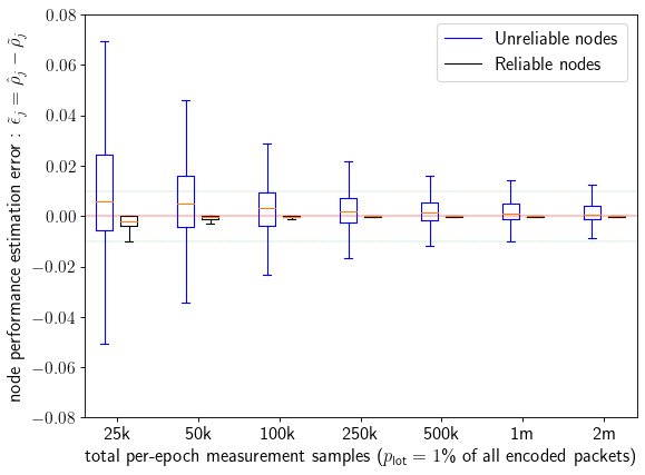
As shown in the figure, the reliability estimation error is consistently small for reliable nodes (black boxes), becoming negligible once \(100\)k or more measurement samples are used. The estimation error is larger for unreliable nodes but decreases with more samples: with \(25\)k samples the error range exceeds \(7\%\) of overestimation and \(5\%\) underestimation, while with \(2\) million samples the error is contained within \(\pm 1\%\). Note that nodes are rearranged in the mixnet each epoch and measured independently, so we expect per-epoch estimation errors to average out when reliability is tracked across many epochs.
Adversarial setting. We next evaluate the proposed node reliability estimation protocol under adversarial conditions. We consider an adversary that controls a set \(A\) of malicious nodes and aims to degrade the measured reliability of a set \(T\) of honest and reliable target nodes. The sizes \(|A|\) and \(|T|\) range (independently) from a single node up to \(40\%\) of two non-adjacent mixnet layers (\(32\) out of \(80\) nodes per layer). To attack a target node, an adversarial node must share an edge with the target—either as its predecessor or successor. If the adversary is the successor, it simply drops packets coming from the target without recording them in its tag-commitment. If the adversary is the predecessor, it registers the received packet tags in the tag-commitment, but drops the packets instead of forwarding them to the target. The goal of the attack is to degrade the measured reliability of the targets relative to their true reliability. The more the protocol underestimates the reliability of the target nodes, the more effective the attack. The adversary’s cost is the “opportunity cost” incurred from its own degraded measured reliability, due to having dropped packets. The attack is thus more costly when the protocol assigns a lower reliability score to adversarial nodes than what they would have received had they behaved honestly.
We run \(510\) simulations with various combinations of \(|A|\) adversaries and \(|T|\) targets, set independently to values \(1\leq |T|\leq 64\) and \(1\leq |A|\leq 64\). In each experiment, we compute the adversarial cost for the \(|A|\) malicious nodes \(c_A = |A| - \sum_{i \in A} \hat{\rho}_i\) and the cost imposed on the \(|T|\) targets \(c_T = |T| - \sum_{j \in T} \hat{\rho}_j\). We show in Fig. 5 a sample per experiment, situated according to the resulting target and adversarial costs \(c_T\) and \(c_A\). Note that the overall attack scale increases proportionally with \(|A|\times|T|\), since this determines the number of links on which packets are dropped—and thus the potential magnitude of \(c_A\) and \(c_T\). This results in \(c_A\) and \(c_T\) values ranging from below \(10^{-2}\) to above \(10\). We use log scale to represent this wide range in Fig. 5.
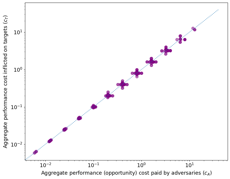
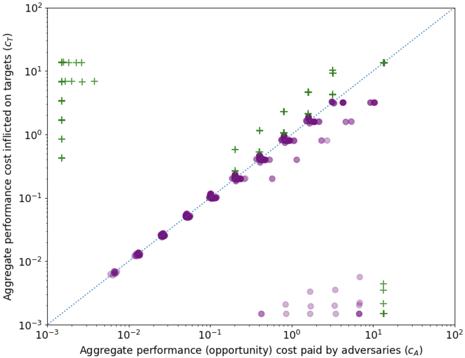
Each simulation result is plotted as a point with coordinates \((c_A, c_T)\). As shown, the results cluster closely around the diagonal \(c_A = c_T\), indicating that, by engaging in the attack, the malicious nodes incur a combined reliability penalty roughly equal to the degradation they inflict on the target set—even in scenarios where \(40\%\) of a target’s predecessors and/or successors are adversarial.
Combining Adversarial and Unreliable nodes. We finally examine scenarios where some nodes not involved in the attack are unreliable. Similarly to the previous case, we compute the adversarial cost for \(|A|\) malicious nodes (\(1 \leq |A| \leq 64\)) as \(c_A = |A| - \sum_{i \in A} \hat{\rho}_i\) and the cost imposed on the \(|T|\) targets (\(1 \leq |T| \leq 64\)) as \(c_T = |T| - \sum_{j \in T} \hat{\rho}_j\). We run \(630\) simulations. Each simulation run produces a result sample \((c_A, c_T)\) that we represent as a dot in a scatter plot. We represent scenarios with large number of adversaries with a different symbol to better evaluate the impact of high corruption rates. Purple circles represent scenarios where adversaries control at most \(20\%\) (\(16\) out of \(80\) nodes) of any layer. Green ‘+’ signs correspond to simulations where adversaries make up \(40\%\) (\(32\) out of \(80\) nodes) of at least one layer. The results are shown in Fig. 6, where we can see that adversary and target penalties are still symmetric in the majority of scenarios. We can see that \(c_A \approx c_T\) in all scenarios below a certain scale. As the attack scale (proportional to \(|A|\)x\(|T|\)) increases however, there are increased chances that unreliable nodes affect the measured reliability of either adversaries or targets, making the attack cost asymmetric. This happens in particular when the combination of attack-related drops and unreliability affects the median incoming or outgoing link reliability of a node, i.e., when more than half of a node’s incoming or outgoing links have sub-par performance for one or another reason. This makes the node be labeled as unreliable and increases the attribution of drops to that node. This can more easily happen to targets that are under attack from a large number of adversaries in an adjacent layer, as well as to adversaries that attack a large number of targets. The considered level of unreliability is not helpful for adversaries that control up to \(20\%\) of any layer (purple circle symbols). In these cases, at best the adversary pays a symmetric penalty (results on the diagonal, for which \(c_A \approx c_T\)), while in other instances it pays a higher cost than the target (circles below the diagonal for which \(c_A > c_T\)). In some instances the adversary pays a large penalty without the attack having an effect on the target (samples on the bottom of the figure for which \(c_A \gg c_T\)).
5 Related Work↩︎
Mixnets for voting. A key use case for mixnets in the literature is electronic voting [7], [29], [30], where the goals are to ensure both unlinkability between voters and their ballots, and the verifiability of the final tally. In such applications, mixnets must offer strong integrity guarantees: each client is authorized to send exactly one well-formed ballot (typically authorized by some form of credential), and mix nodes are required to prove that they correctly process every packet without dropping, injecting, altering, or substituting any messages. These guarantees are achieved by routing all transmissions through a public broadcast channel and requiring per-batch NIZK shuffle proofs [31] to demonstrate that mix node outputs are valid permutations of their inputs. This supports high-assurance verifiability but introduces latency and communication costs only acceptable in voting applications.
Mixnets for messaging. Early mixnets were designed for high-latency messaging (email) and implicitly assumed that mix nodes were reliable [22], [32], [33]. Most modern designs, including cMix [34], Vuvuzela [35], Stadium [9], and Groove [36] similarly assume highly reliable servers and do not incorporate mechanisms to estimate node reliability. A few proposals do consider reliability properties. The Atom mixnet [8] uses lightweight “trap” ciphertexts to detect faulty behavior, but its latency (28 minutes for one million 32-byte messages) scales with message number and size. XRD [10] improves on Atom’s scalability with aggregate hybrid shuffles and identifies misbehaving servers via NIZKs, but its latency scales linearly with the number of Byzantine users. Karaoke [37], the fastest in this category (6.8s for two million clients), uses Bloom filters to detect dropped messages but treats all drops as adversarial and otherwise assumes perfectly reliable servers; its focus is on deanonymization effects of unreliability rather than on scoring node reliability. Across these systems [8], [10], [37], latency and broadcast overhead grow with client message volume. Our scheme instead runs reliability estimation a posteriori, leaving packet-forwarding latency unaffected, and keeps broadcast overhead constant for a fixed topology and target accuracy, regardless of traffic volume.
Continuous-time mixnets. Loopix [13] is not round-based: it processes packets individually with random per-hop delays [38], [39], enabling clients to configure latency profiles [40] for different applications. This makes Loopix well-suited for low-latency use, but it provides no node-reliability mechanism. The Nym mixnet [2], based on Loopix, currently relies on centralized network monitors that loop packets through the mixnet to compute node scores; forthcoming work [41] highlights weaknesses of this centralized approach.
Mixnet reliability and accountability. The idea of estimating a mix node’s reliability using a reputation score was first introduced by Dingledine et al. [19], who proposed a scheme relying on semi-trusted witnesses to verify whether nodes behave correctly. However, their model does not account for active adversaries attempting to manipulate reliability measurements. Subsequent work [17] eliminates the need for witnesses by using test measurements and failure reports, which are tied to reputation, to construct mix cascades that can detect packet drops or substitutions. This design, however, is vulnerable to so-called “creeping death” attacks, where adversaries strategically bias measurements to gradually erode the reputation of honest nodes more than that of malicious ones. Our protocol addresses this limitation by ensuring that adversarial nodes incur reputational penalties that are proportional to the harm they inflict on their targets.
More recent proposals [12], [20] either treat any packet loss as malicious or rely on trusted auditors. The “trip-wire” technique from verifiable mixnets [30], used by [11], [12], resembles our measurement packets in employing indistinguishable test packets, but yields only a binary outcome rather than a representative sample. Our VRF-based measurement packets, by contrast, enable quantitative link and node reliability estimation that reflects user experience.
6 Conclusion↩︎
We have presented the first decentralized, scalable, low-latency scheme for estimating the reliability of a mixnet’s links and nodes. Our link reliability estimation protocol relies on covert measurement packets and a novel VRF-based routing primitive that enforces adherence to the mixnet’s routing policy, preventing malicious clients from biasing paths. The resulting link estimates are combined into node reliability scores that identify underperforming mix nodes with optimal communication overhead.
We empirically evaluated our scheme via simulation. In a Nym-like network with three routing layers and \(80\) nodes per layer, 1 million measurement packets suffice to obtain accurate estimates in both unreliable and adversarial settings. A central insight is that, for a fixed topology and target accuracy, the required number of measurements remains constant as client traffic grows, making the protocol overhead independent of traffic volume. Unlike heavy-weight verifiable mixnets, our design imposes no latency on packet delivery (verification runs a posteriori) and only a small fraction of packets, with minimal per-packet information, ever reaches the broadcast channel.
Although designed for continuous-time mixnets, our protocols can also apply to batch-based systems, since they operate over epochs, and to alternative graph topologies as long as the routing policy is public. The number of links determines the number of measurements required: free routes are the most expensive, parallel cascades the cheapest. Free routes also yield the strongest node scoring, tolerating nearly half of all nodes being adversarial, because every node is predecessor and successor of every other node; cascades on the other hand cannot attribute link drops at all, since each node has only one predecessor and successor.
In terms of future work, interesting directions include further exploring the trade-off between the utility-maximizing and fully-malicious settings with respect to communication overhead, and analyzing griefing attacks on node reliability estimation, where an adversary sacrifices its own reliability to harm honest nodes.
Acknowledgments.↩︎
The authors would like to thank Leif Ryge for early ideas of ‘secret shopper’ traffic to measure the performance for Tor, and further discussions with Jeff Burdges and Leif Ryge for applying this idea in the context of mixnets. We’d like to thank Dan Boneh and Nym advisors Bart Preneel, George Danezis, and Ben Laurie for discussions, as well anonymous reviewers for extensive comments. This research was supported in part by CyberSecurity Research Flanders with reference number VR20192203 and by Nym Technologies SA.
Use of AI-based tools: ChatGPT and Claude were used in the final stages of this paper’s editing, to improve the readability and flow of the text, and to correct typos.
7 Proof of Theorem 1↩︎
For reference we recall our notations in Table ¿tbl:tab:notation? and our underlying packet construction as illustrated in Figure 3.
Proof. (I) The key part in proving the statement is to demonstrate that the values used for the underlying mixnet encoding \(\tilde{r}_i\) are indistinguishable to random values that the client would select independently. The mechanism we use for the special headers is an extension of the Sphinx encoding and hence its security can be argued as in [16]. For completeness we provide the main argument below. The main dependency is on the Decisional Diffie Hellman assumption and the random oracle model. For simplicity we argue first only the case that a single credential is used to send a single packet via a gateway. Consider the \(i\)-th hop of that packet. This involves the values \(\alpha_i = \alpha_{i-1}^{b_{i-1}}\) and \(y_i\), the public-key of the \(i\)-th node.
We show how to incorporate a challenge for the Decisional Diffie Hellman assumption \(\langle g, a, b, c\rangle\) into the encoding calculation. We set the credential key \(\alpha\) to be \(a\) and the node public-key \(y_i\) to be equal to \(b\). It follows that the value \(\tilde{r}_i\) can be calculated as a function of the DDH challenge by \(H(\mathsf{rnd}, c^e)\) where \(e = b_0\ldots b_{i-1} \cdot r_\mathrm{pkt}\). Conditional on \(e\neq 0\), it follows that \(\tilde{r}_i\) is uniformly random, unless the adversary queries the value \(c^e\) to the random oracle. Note that this event can only happen with non-negligible probability in the case the challenge \(\langle g, a, b, c\rangle\) is a DDH tuple (as in the other case, the value \(c\) is random and hence can only be predicted with negligible probability by the adversary). As a result, if the adversary queries \(c^e\) we can readily build a distinguisher by examining the random oracle queries of the adversary. Specifically, the distinguisher can test each query \(q\) for \(q = c^{e}\) and output \(1\) if this is the case while producing \(0\) otherwise. It is easy to see that this algorithm will produce \(1\) with non-negligible probability when the tuple \(\langle g, a, b, c\rangle\) follows the DDH distribution while it will produce \(0\) with overwhelming probability whenever \(\langle g, a, b, c\rangle\) is a random tuple. Finally, observe that the probability that \(e=0\) is negligible given the randomness of the constituent values in the random oracle model.
It follows that the special header value \(\alpha\) can be simulated independent of the packet and its payload under the pseudorandomness of the VRF, the DDH and in the random oracle model, hence as a result the only advantage gained by the adversary can be drawn by the underlying encoding which is assumed to be secure. Finally, note that the above argument generalizes via a hybrid argument in a straightforward manner to the case that there are multiple clients sending multiple packets.
(II) The argument is similar to case (I). Recall our encoding mechanism introduces the values \(\alpha_0, \alpha_1, \ldots, \alpha_\nu\) that accompany each packet when they are sent over the network. As mentioned already, this is a sequence of blinded values that follow the Sphinx construction and hence the privacy proof would be identical. For completeness, the key argument is the following. Consider the two values \(\alpha^*_0, \alpha^*_1\) originating from the packet processing performed by the node. We consider the two cases in the theorem statement. When the packets are processed it holds that there are two exponents \(e_0,e_1\) such that \((\alpha^*_0, \alpha^*_1) = (\alpha_0^{e_0}, \alpha_1^{e_1})\). The indistinguishability of \((\alpha^*_b, \alpha^*_{1-b})\) to \((\alpha^*_{1-b}, \alpha^*_{b})\) boils down to the pseudorandomness of the \(e_0,e_1\) exponents which can easily argued in a similar way as above under DDH and the random oracle model.
(III) The statement asks for the pseudorandomness of the values \(r_0,\ldots,r_{\nu-1}\), even in the case that the values \(vk, \alpha, y_0\) are adversarially chosen. Note that in this case we cannot rely on the DDH assumption or the properties of the VRF. Instead the key observation is that each value \(r_i\) depends on the public nonce value via the random oracle as well as some other value \(s_i\) that as long as it is unique, \(r_i\) would be an independently sampled value. To prove this we consider the event that there are two values \(s = g^{e}, s'=g^{e'}\) in this sequence that are equal, i.e., \(e=e'\). Depending on the step when these values have been calculated the exponents will be a product of a number of values some of which are committed by the adversary, e.g., the discrete logarithm of the key of an adversarial gateway, the discrete logarithm of a credential’s randomization key \(\alpha\) as well as values produced by random oracle evaluations of such values e.g., the blinding exponents \(b_0, b_1, b_2,\ldots\) and the keys of the mix-nodes. Conditional on no collisions in the random oracle \(H(\cdot)\) or the VRF function, all these individual values involved in \(e,e'\) are distinct and, in case they are not outputs of the random oracle, are committed prior to the production of \(\mathsf{nonce}\). Based on this, it follows that the event \(e=e'\) would imply the event that \(z_1 \cdot z_k \cdot h_1 \ldots h_t = 1\) where \(h_1,\ldots,h_t\) are random oracle outputs that depend on \(\mathsf{nonce}\) and \(z_1,\ldots, z_k\) values selected by the adversary. It is easy to see via generalized birthday problem [42] that this would require subexponential overhead in the worst-case (note in our setting \(t\) is a small constant).
(IV) This statement follows easily due to the fact that the only difference between measurement and non-measurement packets is in the calculation of the \(\alpha_0\) value: in the case of a non-measurement packet this value is equal to \(\alpha^{r_\mathsf{pkt}}\), while in the case of a measurement packet it is equal to \(g^{r_\mathsf{pkt}}\). In the view of a relay node, the exponentiation by the (hidden) value \(r_\mathsf{pkt}\) results in a full randomization of the resulting element within the base group (with the precondition \(\alpha\neq 1\)); as a result the two cases are indistinguishable assuming the security of the VRF function. ◻
8 Approaches to setting \(\hat{\beta}_e\)↩︎
Here we propose and review three heuristic approaches to setting values for \(\hat{\beta}_e\), which defines the fraction of drops \({d}^*_e\) in link \(e=(i,j)\) that are attributed to successor \(j\), while the remaining \((1-\hat{\beta}_e)\cdot {d}^*_e\) drops are attributed predecessor \(i\). We assume reliable link transmissions such that no packets are dropped in link \(e=(i,j)\) if both \(i\) and \(j\) are online and functioning correctly.
8.1 Naive approach: \(\hat{\beta}_e =1\)↩︎
A simple approach is to “blame the receiver,” which corresponds to setting \(\hat{\beta}_e =1\) for all edges \(e\). The rationale for this approach is that most of the hard work of processing a packet (deriving the decryption key and checking the packet tag for replay) is done by the time a node \(i\) is able to store the packet tag in its tag-commitment. Thus, if a packet is lost in link \((i,j)\), chances are that the blame is with \(j\), who failed to be online or otherwise to process the packet. This naive model performs quite well in scenarios where all link drops are due to random failures by honest but unreliable nodes, since in practice chances are that the drop is due to the receiving end \(j\) being either offline or congested.
Such model is however easily subverted in a strategic adversarial setting: a malicious node \(i\) can selectively drop received packets (after storing their tag in the tag-commitment) destined to one or more target successors \(j\), in order to unfairly degrade their measured reliability \(\hat{\rho}_j\). Given a mixnet with layer width \(W\), an adversary that controls a set of \(i \in A\) nodes in a layer can degrade the measured reliability \(\hat{\rho}_j\) of any number of nodes \(j\) in the succeeding layer, by up to \(\frac{|A|}{W}\) at zero cost for the adversarial nodes in terms of lower measured reliability \(\hat{\rho}_i\) for malicious nodes \(i \in A\).
8.2 Symmetric approach: \(\hat{\beta}_e =\frac{1}{2}\)↩︎
An alternative approach to penalize and discourage such adaptive malicious behaviour is to define node reliability considering that half the ‘blame’ for drops in link \(e=(i,j)\) is with \(i\), and the other half with \(j\), i.e., setting \(\hat{\beta}_e =\frac{1}{2}\) for all links \(e\). This symmetric attribution approach is effective at discouraging malicious packet drops as any drop now affects the reliability of the adversarial node comparably to that of its target, which can be either a predecessor or a successor of the attacker. A practical concern in cases where no attack takes place is that the symmetric attribution of blame results in a lowered reliability \(\hat{\rho}_i\) for the predecessors \(i\) of nodes \(j\) that are either offline or congested and unable to process all the received traffic – a scenario that may not be rare. This may unfairly degrade \(\hat{\rho}_i < {\rho}_i\) for reliable nodes \(i\) at the expense of overestimating \(\hat{\rho}_j > {\rho}_j\) for unreliable nodes \(j\).
Consider a case where \(j \in F\) nodes in a layer of width \(W\) go offline shortly after processing a few packets,12 while all their predecessors \(i\) are honest and reliable throughout the entire epoch, i.e., \({\rho}_i = 1\) for all nodes in the preceding layer. Attributing drops symmetrically causes \(\hat{\rho}_i\) to be unfairly degraded by \(\frac{|F|}{2W}\), while offline nodes \(j\) unfairly get credit for processing half the traffic sent their way, and their measured reliability may be as high as \(\hat{\rho}_j \approx \frac{1}{2}\) while in truth \({\rho}_j \approx 0\).
8.3 Threshold approach: \(\hat{\beta}_e \in \{0, \frac{1}{2}, 1\}\)↩︎
The threshold approach aims to: (i) eliminate the unfair degradation of measured reliability for reliable nodes due to successors being offline or congested, or predecessors being consistently faulty; while (ii) still symmetrically penalizing malicious nodes that conduct selective dropping attacks to degrade the estimated reliability of honest, reliable predecessors or successors. This is achieved by assigning values to \(\hat{\beta}_e\) that take into account node reliability across its whole set of incoming or outgoing edges. The reliability \(\hat{\rho}_e\) of each edge is computed with Eq. 3 .
Median incoming and outgoing reliability. Given \(\hat{\rho}_{e} = \frac{{s}^*_e}{{s}^*_e + {d}^*_e}\) for each edge \(e\), we denote by \(\bar{\rho}^{\mathsf{in}}_j =\) med\(\{\hat{\rho}_{(i,j)}\) for \(i \in P(j)\}\) the weighted median of incoming link reliability for node \(j\), and by \(\bar{\rho}^{\mathsf{out}}_j =\) med\(\{\hat{\rho}_{(j,k)}\) for \(k \in S(j)\}\) node \(j\)’s median outgoing link reliability. The node weight in the median computation is given by the share (relative to the full layer) of incoming or outgoing traffic routed by that node. In the case of links between mixnet layers, the node weight is determined by the routing policy. All the nodes in a layer count the same weight \(\omega^{\mathsf{out}}_i =\omega^{\mathsf{in}}_j = \frac{1}{W}\) when the routing policy is uniform. This is not necessarily the case for gateways, whose weight is instead proportional to their share of sent measurement traffic received by mix nodes in the first layer (i.e., \(\omega^{\mathsf{out}}_g = \frac{\sum_i {s}^*_{(g,i)}}{\sum_x \sum_i {s}^*_{(x,i)}}\) when computing \(\bar{\rho}^{\mathsf{in}}_i\) for \(i \in S(g)\)), or received measurements from mix nodes in the last layer (i.e., \(\omega^{\mathsf{in}}_g = \frac{\sum_k {s}^*_{(k,g)}}{\sum_x \sum_k {s}^*_{(k,x)}}\) when computing \(\bar{\rho}^{\mathsf{out}}_k\) for \(k \in P(g)\)). Threshold criteria. Let \(\bar{\tau}\) be a threshold for the median reliability that nodes are expected to achieve at a minimum when participating in the mixnet (we use \(\bar{\tau}=0.99\) in our experimental evaluation). The \(\hat{\beta}_e\) is set per edge \(e=(i,j)\) and it takes values in \(\{0,\frac{1}{2}, 1\}\), according to the following criteria:
\(\bullet \,\,\) \(\hat{\beta}_{(i,j)} = 1\): if \(\bar{\rho}^{\mathsf{in}}_j < \bar{\tau}\) and \(\bar{\rho}^{\mathsf{out}}_i \geq \bar{\tau}\) (\(j\) has sub-par median incoming reliability \(\bar{\rho}^{\mathsf{in}}_j\) while \(i\) has above-threshold outgoing median reliability \(\bar{\rho}^{\mathsf{out}}_i\)). If \(\sum_i {s}_{(i,j)}^* = 0\) then \(\hat{\beta}_{(i,j)} = 1\) for any value of \(\bar{\rho}^{\mathsf{out}}_i\).
\(\bullet \,\,\) \(\hat{\beta}_{(i,j)} = 0\): if \(\bar{\rho}^{\mathsf{in}}_j \geq \bar{\tau}\) and \(\bar{\rho}^{\mathsf{out}}_i < \bar{\tau}\) (\(j\) has above-threshold median incoming reliability while \(i\) is showing low reliability in more than half of its outgoing links).
\(\bullet \,\,\) \(\hat{\beta}_{(i,j)} = \frac{1}{2}\): if \(\bar{\rho}^{\mathsf{out}}_i, \bar{\rho}^{\mathsf{in}}_j \geq \bar{\tau}\) (both \(i\) and \(j\) have above-threshold median reliability), or \(\bar{\rho}^{\mathsf{out}}_i, \bar{\rho}^{\mathsf{in}}_j < \bar{\tau}\) (both \(i\) and \(j\) have sub-par median reliability).
Using median values \(\bar{\rho}^{\mathsf{in}}_j\) and \(\bar{\rho}^{\mathsf{out}}_j\) to infer whether a node is performing adequately across the board makes the approach robust to adversarial settings, up to the point where the adversary controls enough resources to affect median values. In the case of uniform routing and \(W\) nodes per mixnet layer this means controlling \(\frac{W}{2}\) nodes in a layer; while in the case of gateways it involves controlling gateways that combined send half the total client traffic or that receive half of all the measurement packets.
9 Mixnet Simulator↩︎
This section provides a description of the simulator we implemented13 and used to conduct an empirical analysis of the proposed reliability estimation protocol. The scripts are in Python and use the SimPy library to handle events such as packet creation, packet sending, receiving and dropping. This section provides extensive details on the features, parameters and experimental setups used in to obtain the results presented in previous sections, as well as additional experiments excluded from the main body due to page limit.
9.1 Clients and Encoded Packets↩︎
The simulator runs clients that encode and send packets throughout a simulated epoch of one hour. Packet generation by clients follows a Poisson process with a configurable rate of \(\lambda\) packets per second. Each encoded packet is a measurement packet with (globally configurable) probability \(p_\mathsf{lot}\). The rest are data packets addressed to other (randomly chosen) clients or cover traffic that clients send to themselves. Packets’ routes are selected according to a uniform routing policy, considering a mixnet with \(L=3\) layers and \(W=80\) mix nodes per layer, as well as \(W_G=80\) gateways.We consider that legitimate client traffic is uniformly distributed over all gateways and also addressed in equal measure to recipients in all gateways. The encoded delay per packet per mix node is exponentially distributed with average \(50\)ms, and we additionally consider \(40\)ms of transmission time in each link and \(2\)ms of packet processing time at the gateways.
9.2 Reliable, Unreliable and Malicious Nodes↩︎
In the simulations we treat gateways and mix nodes equally in terms of reliability, failure modes and malicious behaviour, and thus refer to all \(80\) gateways and \(240\) mix nodes indistinctly as ‘nodes’ that receive packets from their predecessors and forward them to their successors, sometimes dropping packets if they are adversarial or not fully reliable. Packets may be dropped by a node before or after the packet tag is stored in the node’s tag-commitment. If a packet is dropped before storing, it is considered that the drop happened in the node’s incoming link. If the drop happens after storing then it is accounted for in the node’s outgoing link. Nodes can have various types of behaviours:
\(\bullet \,\,\) Reliable nodes are honest and function perfectly: they are always online and correctly process all the received packets without dropping any of them.
\(\bullet \,\,\) Unreliable or faulty nodes are non-adversarial but subject to failures that cause packet drops. The possible failures include: (a) going offline for some (exponentially distributed) period of time, dropping any packets that were inside the node at the moment of going offline, as well as failing to receive new packets while offline; (b) becoming congested due to having a limited throughput and dropping packets on incoming links when the incoming packet rate exceeds the node’s throughput; (c) suffer from random glitches that cause packet drops in incoming or outgoing links with a certain probability.
\(\bullet \,\,\) Malicious nodes are always online and have high throughput but they purposefully drop all or a fraction of packets in links with selected predecessor or successor targets, in order to degrade the reliability estimates \(\hat{\rho}_j\) for those targets.
9.3 Simulation Outputs↩︎
Once the epoch finalizes, the simulator logs in .csv files the outputs of the sampling protocol, including the \({s}^{*}_e\), \({d}^{*}_e\) counts per link \(e\) as well as \(\hat{\rho}_j\), \(\bar{\rho}^{\mathsf{in}}_j\), \(\bar{\rho}^{\mathsf{out}}_j\) estimates for every node \(j\). In addition, the simulator logs packet counts for all edges and nodes that would not be available in an actual deployment – but that are available in a simulated environment and useful for evaluation purposes. This includes \({s}_e\), \({d}_e\), \({\rho}_e\), and \({\beta}_{e}\) for all edges as well as \({\rho}_j\) for all nodes and gateways. We evaluate the proposed reliability estimation protocols by comparing the \(\hat{\rho}_j\) output by the protocol to the underlying ground truth reliability \({\rho}_j\), both in settings where packet drops are due to random failures and settings where packet drops are malicious.
9.4 Simulation Runtime↩︎
The runtime of a simulation is proportional to the number of packets encoded and routed in the full simulation. Each packet triggers a number of events, first as it is created by a client and then every time it is sent or received by an intermediary routing (or dropping) the packet. We perform simulations with a total of encoded packets between \(2\) million and \(200\) million, which require, respectively, between \(15\)-\(20\) minutes and \(30\)-\(36\) hours to complete. Simulations are CPU intensive (each simulation fully utilizes a CPU) but require little memory.
9.5 Experimental Setup: Honest but Unreliable Setting↩︎
In this setup we simulate scenarios where in each layer \(40\) nodes (half the layer) are reliable and the other \(40\) are (potentially) unreliable in various ways. To test the effect of different modes and degrees of failure we consider:
\(\bullet \,\,\) \(32\) unreliable nodes per layer (\(40\%\) of the layer) may go offline during the epoch. Each of these nodes toggles between being online and offline for exponentially distributed lengths of time, with average \(90\) minutes online and \(10\) minutes offline; i.e., on average, these nodes are online \(90\%\) of the time.
\(\bullet \,\,\) \(4\) unreliable nodes per layer (\(5\%\) of the layer) have limited throughput, with one of them having a throughput equal to the average per-node incoming packet rate (and thus only dropping some packets when traffic is higher than average), and the other three having throughput that is \(\frac{1}{2}\), \(\frac{1}{4}\), and \(\frac{1}{8}\) of the average incoming packet rate (and thus dropping, respectively, about \(\frac{1}{2}\), \(\frac{3}{4}\), and \(\frac{7}{8}\) of incoming packets).
\(\bullet \,\,\) The final \(4\) unreliable nodes per layer (\(5\%\) of the layer) randomly drop some packets. One of these nodes drops \(1\%\) of the incoming packets, another drops \(1\%\) of outgoing packets, a third drops \(20\%\) of incoming packets and the last drops \(20\%\) of outgoing packets.
We set the probability of a packet being a measurement to \(1\%\), i.e., \(p_\mathsf{lot}=0.01\). We vary the total amount of packets encoded by clients to study the node reliability estimation accuracy relative to the number of measurement samples throughout the epoch. The results are shown in Figure 4.
9.6 Experimental Setup: Adversarial Settings↩︎
To simulate adversarial settings we consider scenarios with \(A=\{1, 2, 4, 8, 16, 32, 64\}\) adversaries and \(T=\{1, 2, 4, 8, 16, 32, 64\}\) targets. We only consider node assignments to layers that are most favorable to the adversary, i.e., where all \(A\) adversarial nodes are in layers adjacent to all the \(T\) targets, either as predecessors, as successors, or both. In cases where all \(A\) nodes are in a single layer, the \(T\) nodes may be all in the preceding layer, all in the succeeding layer or, for \(T>1\), distributed as \(\frac{T}{2}\) in the preceding and \(\frac{T}{2}\) in the succeeding layers. In cases where the \(A\) nodes are distributed among two layers, we consider that all \(T\) targets are in the layer between the adversaries, with \(\frac{A}{2}\) as predecessors and the other \(\frac{A}{2}\) as successors of the \(T\) targets. For \(64\) adversaries or targets we only consider scenarios where they are split over two layers (rather than all in one layer). We consider that the \(A\) adversaries maximize the attack impact by dropping all (rather than just some) of the packets in the edges shared with the \(T\) targets – while not dropping any packets on edges shared with non-targets. Targets are reliable nodes that do not drop any packets and thus have a true reliability of \(100\%\). For the remaining ‘vanilla’ nodes, which are non-adversarial and non-targets, we consider two cases: one where they are all reliable, and another where \(30\%\) of the nodes in each layer are potentially unreliable (results reported in Section [sec:perf-adversarial]). The second case uses a setup almost identical to the one described in Section 9.5, with the only difference being that only \(16\) (rather than \(32\)) unreliable nodes per layer may go offline during the epoch. We consider scenarios with a total of \(2\) million measurement packets per epoch of one hour.
10 Protocol overhead evaluation↩︎
We evaluate the overhead introduced by the proposed protocols in terms of the data that must be broadcast per epoch, the data that must be persisted long-term on a blockchain, and the computational overhead of VRF-based routing. We assume that several variables required by our protocols are already publicly available for the baseline operation of the mixnet, even before introducing any reliability measurement mechanisms. This includes: the mixnet topology definition, per-epoch node-to-layer assignments, node public keys (used for signing broadcast data and decrypting packets), node reward information, client subscriptions, and spent credentials (corresponding to step B.1 in Fig. 2). We therefore focus solely on the additional overhead incurred by the reliability estimation protocol, as summarized in Table 1.
We consider a setup in which \(100\) million packets are routed per epoch, of which \(1\) million (\(1\%\)) are measurement packets. The mixnet comprises \(80\) gateways and \(240\) mix nodes, divided across three layers of \(80\) nodes each. The communication complexity when using Merkle trees as tag-commitments is discussed in Sect. 3.1. Here we assume Bloom filters are used for tag-commitments, thereby making steps B.4 and B.6 in Fig. 2 unnecessary. The data that must be broadcast in each epoch to compute reliability scores includes:
Bloom filters: Each node must broadcast its tag-commitment at the end of the epoch (step B.2 in Fig. 2). In the considered setup, a mix node is expected to route \(1/80\) of the total traffic, amounting to \(1.25\) million packets. Assuming a false positive rate of \(10^{-5}\), this results in a Bloom filter of approximately \(3.5\) MB in size.14 With \(240\) mix nodes, the total Bloom filter data adds up to \(840\) MB. The \(80\) gateways can use smaller Bloom filters, as they only need to record received measurement packets. Assuming a maximum of \(100,000\) received measurements per gateway, each filter would be about \(300\) KB, totaling \(24\) MB across all gateways.
Merkle Trees: Each node must broadcast a tag-commitment at the end of the epoch (step B.2 in Fig. 2) which is merely 32 bytes (the Merkle tree root) assuming SHA256 as the underlying hash function. Subsequently, each node should open the tags that correspond to the measurement packets (step B.4 in Fig. 2). Assuming a maximum of 100,000 measurements, for mix nodes, this would require 17 hashes per membership proof resulting in a total of \(55\) MB of data per node.
Per-packet openings: Gateways broadcast an opening per measurement packet (step B.3 in Fig. 2), each of size 388 bytes. For \(1\) million measurement packets, this adds up to 388 MB of broadcast data.
Proofs of no-skipping: Each opening for a non-measurement position is 132 bytes. Given a total of 99 million non-measurement packets per epoch, we consider an adversarial gateway that hides one measurement packet. By requiring proofs for \(99\cdot 10^6 \ln (1-.01)^{-1} \approx 10^6\) non measurement positions, the probability of detecting the omission is at least \(1\%\). The resulting data overhead is \(132\) MB, and such a gateway would be caught on average within \(100\) epochs.
We consider that the computed reliability scores for all nodes and gateways are stored persistently in the blockchain to act as a historical record of their measured reliability. Assuming a precision of four decimal places, this requires \(2\) bytes per node and gateway, resulting in a total of \(640\) bytes per epoch for \(240\) nodes and \(80\) gateways. Additional protocol parameters that must be stored on-chain, such as \(p_\mathbf{lot}\) and \(\bar{\tau}\), occupy only a few extra bytes and do not require updates every epoch.
| Broadcast | Per item | Amount | Total data |
| Packet openings | 388 B | 1 million | 388 MB |
| Bloom filters mix nodes | 3.5 MB | 240 | 840 MB |
| Bloom filters gateways | 300 KB | 80 | 24 MB |
| No-skipping proofs | 132 B | 1 million | 132 MB |
In terms of computational overhead, based on public benchmarks from Nym for Sphinx packet processing,15 the per-hop latency on a standard Linux server is approximately \(0.32\)ms. We observe that VRF-based routing adds at most the equivalent of a single Sphinx processing step, keeping the total per-hop latency below \(1\)ms. Moreover, combining our scheme with Sphinx allows for further optimizations that can further reduce this overhead. Each packet requires three VRF evaluations, but these can be performed in advance during a preprocessing phase, so they do not affect transmission latency. If packet creation occurs in real time rather than via preprocessing, the three VRF operations would introduce approximately \(1\)ms of additional computation. With simple optimizations, this cost can be reduced to a single VRF evaluation per packet. Aside from these negligible increases in latency introduced by VRF-based routing, our reliability estimation protocols do not affect real-time packet forwarding, as all computationally intensive steps are performed a posteriori—after the packets for an epoch have been delivered—rather than during packet transmission. The protocols are designed to complete within a single epoch, which is easily achievable for epoch durations of one hour (as in the current Nym mixnet) or longer.
References↩︎
This research was supported in part by CyberSecurity Research Flanders with reference number VR20192203 and by Nym Technologies SA.↩︎
Nym (https://nym.com/explorer) currently routes packets with \(500\)ms to \(800\)ms end-to-end latency, including mixing and propagation. Packet processing itself takes under \(1\)ms and is negligible by comparison.↩︎
Due to the lack of low-latency decentralized solutions, the Nym network currently relies on centralized Network Monitors that send loops of traffic through the mixnet to derive node reliability scores.↩︎
Note that each new credential \(c\) allows the client to present a new identity towards gateways, thanks to the credentials’ unlinkability properties.↩︎
Note that this error estimation becomes increasingly inaccurate as \(\rho_e\) approaches zero or one. An accurate confidence interval can be derived following Clopper Pearson [25] (but it has no nice closed formulation as Eq. 5 ).↩︎
As a real-world sanity check, Nym’s reward function [3] can easily be configured for gateways to increase monotonically with all these variables.↩︎
Note that any desired exit gateway distribution may be used here.↩︎
Nym clients currently send a self-loop every \(200\)ms (on average), as well as sending self-loops to fill gaps in a Poisson schedule (packets sent every \(20\)ms on average) when there are no data payloads to send.↩︎
Nodes not actively participating in the mixnet in an epoch need to be tested separately in order to update their reliability scores—a challenge outside the scope of this work.↩︎
In the extreme case where a node \(j\) has zero measurement packets in its tag-commitment for the epoch, i.e., \(\sum_i {s}_{(i,j)}^* = 0\), then the node is marked as having reliability \(\hat{\rho}_j = 0\), and all drops in the edges \((i,j)\) can be safely attributed to \(j\), i.e., \(\hat{\beta}_{(i,j)}=1\).↩︎
Available at: https://github.com/claudia-diaz/artifact-decentralized-measurements-EuroSP2026.↩︎
We use Bloom filter calculators available at https://hur.st/bloomfilter/↩︎