¹

²

Introduction↩︎

Despite the disruption caused by the COVID-19 pandemic and the rapid advances in telecommunication, face-to-face interactions still substantially influence our social life. Research has recently called attention to the importance of face-to-face interactions across multiple frameworks, including creative idea generation and diffusion [1]–[3], information transfer [4], [5], education [6]–[8], psychological well-being [9], and, naturally, epidemic disease spreading [10]. The availability of high-resolution data on face-to-face contacts has allowed researchers to uncover how those interactions display coherent spatio-temporal characteristics across several social contexts. Specifically, face-to-face interactions show universal features, such as the absence of a characteristic scale for contact duration, the switching between low activity periods and high activity bursts, and considerable heterogeneity in interaction behaviors among individuals [11]–[17]. The ubiquity of these features has thus posed the crucial challenge of explaining what mechanisms underlie their emergence.

Modeling frameworks based on mobile agents proved to be a valuable tool to study the organization of human face-to-face interactions. In this scenario, agents move erratically in a spatial environment, and interactions occur every time they get close together [18]. In addition, contacts between agents can be modulated by more complex mechanisms, including their attractiveness [19], [20], their activeness and reachability [21], their pairwise similarity [22], [23], or belonging to the same social group [24]. This class of models gave useful insights to understand the bursty [19] and small-world behavior of face-to-face interactions [25], as well as many social phenomena emerging from them, e.g. disease spreading [26], [27], spatial segregation and echo chamber formation [22], and structural inequalities [24].

Those models, however, are limited as they describe face-to-face interactions only in terms of dyadic relationships between agents. In fact, they adopt a temporal network representation [28], focusing on either the dynamics of dyadic contacts, i.e., links, [19], or the mesoscopic level of social gatherings, i.e., connected components [18], [23]. However, the fundamental structures of face-to-face contacts are many-to-many interactions rather than one-to-one interactions [29]. Recent analyses of high-resolution face-to-face contacts shows indeed that humans do not only interact in pairs but regularly engage in groups involving more than two individuals at the same time [30], a scenario that is better described by higher-order networks [31]. Recent works have investigated the higher-order nature of face-to-face interactions with models based on different social mechanisms, including self-reinforcement, memory, and attribute-related network mechanisms [32]–[34]. Yet, these higher-order network approaches do not incorporate the spatial mobility of agents, and current models based on mobile agents either overlook or fail to capture [20] the spatio-temporal features and the dynamical evolution of groups.

Here, we bridge this gap by introducing a model in which mobile agents interact with each other by forming groups of different sizes. Each group is characterized by an intrinsic degree of social appeal that we call “group attractiveness”. Agents passing in the vicinity of a group choose whether to join it based on its attractiveness, while group members decide whether to stay or walk away. We show how the Group Attractiveness Model (GAM) can reproduce different properties of groups in face-to-face interactions, including their statistics, the correlation in their number, and their temporal duration. Furthermore, differently from low-order approaches, we demonstrate the potential of our model to correctly capture higher-order homophilic patterns not only at the level of pairwise contacts but also at that of groups. Given its predictive power, the Group Attractiveness Model can foster the study of human face-to-face interactions, paving the way for further investigation of how group dynamics at a microscopic scale affects social phenomena at a macroscopic scale.

Results↩︎

The Group Attractiveness Model↩︎

In the Group Attractiveness Model (1), \(N\) agents are placed in a square environment of size \(L\times L\), with periodic boundary conditions, i.e., when an agent crosses the left (top) boundary of the square, it reappears at the right (bottom) boundary. Each agent \(i\) has a value of attractiveness, \(a_i\), which represents how appealing the agent is to the others. Following [19], [20], we operationalize attractiveness as the power of individuals to make others willing to interact with them, without making any assumptions on the social, economic, or behavioral factors that may determine it. The value of attractiveness is sampled from a uniform distribution in the interval \([0,1]\). Agents can be isolated, or they can be part of a group. An agent can decide to interact with the groups surrounding it or to walk away in a random direction. How attractive a group is derives from how attractive its members are. Formally, for each group of agents \(g\), we define its attractiveness as \[a_g = \prod\limits_{j\in g} a_j, \label{eq:GA}\tag{1}\] where index \(j\) runs over all agents forming group \(g\). Note that an isolated agent constitutes a group of one member (group \(g_3\) in 1). Since the attractiveness of an individual does not depend on that of others, the average attractiveness of a group of size \(s\) is \(\overline{a}^s\), with \(\overline{a}\) denoting the average individual attractiveness. Consequently, the group attractiveness scales nonlinearly with its size, with larger groups being, on average, less attractive than smaller ones. At time step \(t\), each agent \(i\) considers the the set of groups, \(\mathcal{N}(i)\), located within a distance \(d\) from it and interacts with all of them with probability \[p_i(t) = \frac{1}{|\mathcal{N}(i)|}\sum\limits_{g\in\mathcal{N}(i)} a_g, \label{eq:eq2}\tag{2}\] Therefore, when an agent chooses to interact with a group of size \(s\), a group of size \(s+1\) is formed at time \(t+1\). Groups in our model thus change gradually, with the addition of one member at a time, a mechanism supported by evidence from real-world human face-to-face interactions [30], [33], [34]. If \(i\) is already part of a group, we consider the group formed by the other members to be part of \(\mathcal{N}(i)\). Therefore, when \(i\) decides to interact, it rejoins the group it was part of, i.e., the group persists in time. Also, when a group partially lies within the scope of an agent, the latter interacts only with those agents that are at a distance smaller than \(d\) (e.g., only one member of group \(g_2\) in 1 is close to agent \(i\), so a group of size 2 is formed between them). When an agent does not interact with its neighboring groups, it makes a step of length \(v\) along a direction given by a randomly chosen angle \(\xi\in [0,2\pi]\), leaving all the groups it was part of in the previous time step. Hence, a group persists in time only when all its members decide to interact with the others [35]. Finally, we assume that agents can be active or inactive. While an active agent can walk or form groups with other agents, an inactive agent neither moves nor interacts with the others. Inactive agents can become active with probability \(r_i\), which we sample from a uniform distribution in \([0,1]\), while active agents that are isolated can become inactive with probability \(1 - r_i\). This further mechanism models the empirical observation that people can leave or join the social context [19] and allows us to distinguish between the individuals that are not in the system from those that are in the system but do not engage in group conversations.

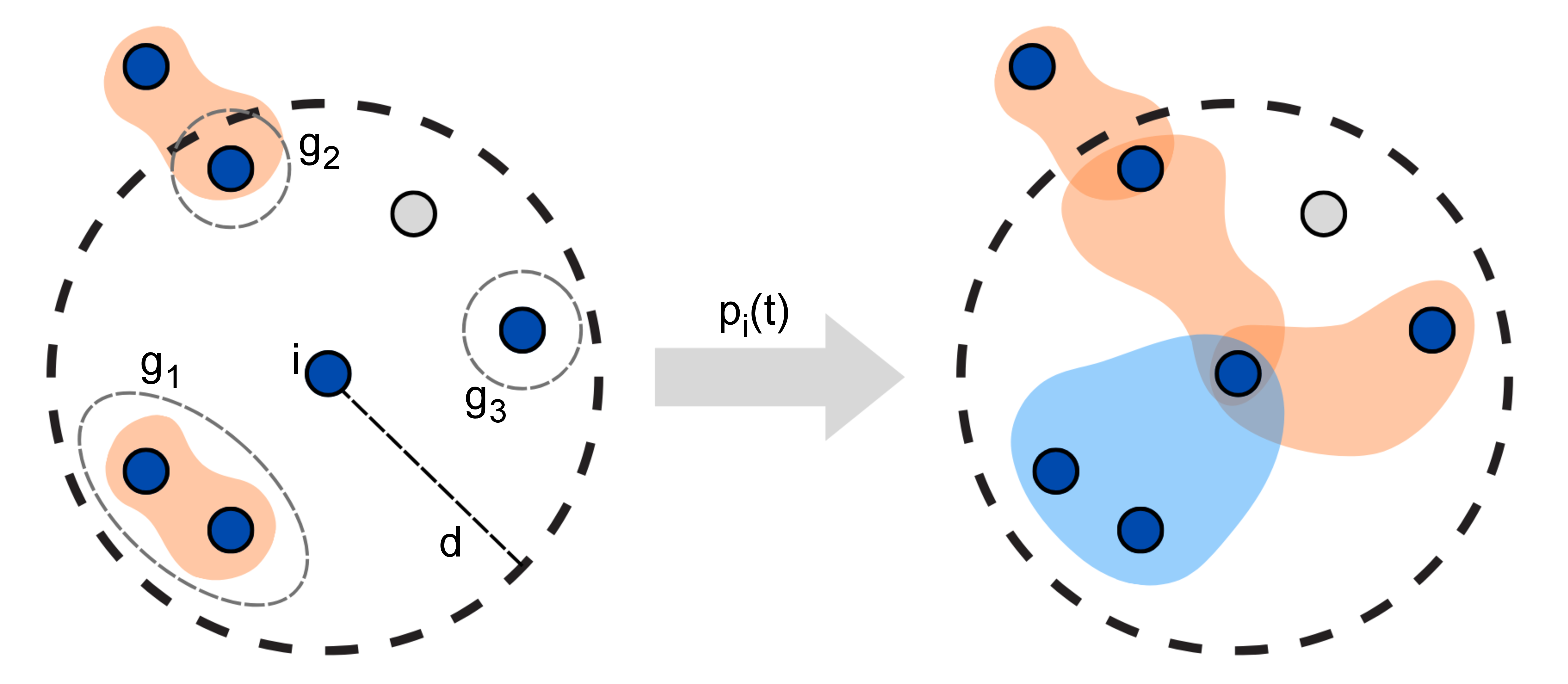
At the end of each time step, the system consists of interacting groups that potentially overlap, i.e., share one or more members, plus a set of agents that do not interact. From a network science perspective, this can be described as a hypergraph [31], which evolves over time [30].

The attractiveness of an agent represents the likelihood that other agents will interact with it when passing by. This likelihood can be influenced by multiple factors, e.g., the fame of an individual, and it may be hard to measure empirically. To avoid introducing any biases, we sample the attractiveness from a uniform distribution. Still, the dynamics of the system may be robust under other choices, such as a normal distribution (see Figs. S1-S2 in the Supplementary Information).

In the Group Attractiveness Model, three different social processes, i.e., joining pre-existing group conversations, remaining in them, and leaving them, are regulated by the average attractiveness of the groups surrounding them. The attractiveness of those groups decrease with their size. Previous research motivates this modeling choice: On the one hand, studies have shown that larger groups involved in exclusive interactions, e.g., conversations, tend to be more impermeable and more repelling, hence less attractive, to passersby [36]–[39]. On the other hand, there is an upper limit on how many individuals can converse [40], after which the conversation splits up into two or more conversations [41], a phenomenon known as schisming [42].

Higher-order statistics of human face-to-face interactions↩︎

To test the capability of the Group Attractiveness Model to reproduce higher-order patterns of human face-to-face interactions, we analyze thirteen high-resolution datasets, ten coming from the SocioPatterns collaboration [11], two from as many experiments in Utah [43], and one from the Copenhagen Network Study [44].

SocioPatterns data report dyadic contacts between individuals facing each other within a 1–1.5 meter range with a high temporal resolution, i.e., 20-second intervals, recorded using Radio Frequency Identification (RFID) devices. The datasets describe the dynamics of contacts between individuals in different social contexts, specifically a primary school (“PS”) [12], a high school (“HS11”, “HS12”, and “HS13”) [15], [17], two scientific conferences (“C16” and “C17”) [45], an art exhibition (“SG”) [13], a hospital (“H”) [46], a village in Malawi (“MV”) [47], and a workplace (“WP”) [48]. Besides contact patterns, the datasets on schools and conferences (six in total) contain information about participants’ gender.

Datasets from the Utah experiments report contacts between pairs of people located 2 meter or less from each other, with a 20-second resolution, in a middle school (“MS”) and an elementary school (“ES”), recorded with Wireless Ranging-Enabled Nodes (WRENs). Data from the Copenhagen Network Study consists of dyadic interactions in a university campus (“UC”), registered every 5 minutes using the Bluetooth technology, which has a range of 10 meters. Here we focus on the six SocioPatterns datasets with gender, and report the analysis of the other six systems in the Supplementary Information.

As all datasets store interactions as dyadic contacts, we first reconstruct group interactions, i.e., face-to-face conversations involving two or more individuals, leveraging the fine-grained temporal information of the data. Specifically, if at a time \(t\) we find all possible dyads among \(s\) individuals, we assume that they are part single group of size \(s\) (see Materials and Methods for details). The statistics of unique groups of different sizes for the ten datasets are shown in 2 and Fig. S1 as black circles. In general, smaller groups are more abundant than larger ones, except for the “C16” and the “UC” dataset (see Table S1 in Supplementary Information).

We now want to verify whether our model is able to reproduce the distribution of unique groups in those social systems. We initialize the model simulation by randomly placing each agent in the environment and setting agents active with probability \(1/2\). We fix \(v=d=1\) and the number of agents \(N\) as the number of individuals forming the largest connected component in the hypergraph of contacts (see Supplementary Information for more details). The simulation stops once the number of groups of size two generated reaches the empirical value. The number of groups of size three or more utterly depends on the agent density. For instance, if the size \(L\) of the environment is significantly large, then agents would rarely get in contact with each other, making the formation of large groups quite unlikely. On the other hand, when agents are close to each other, i.e., when the density is high, it is more likely that agents form groups of various sizes. Hence, we fit the value of \(L\) that best reproduces the group statistics in the dataset (see Supplementary Information for the best-fit values of \(L\) in each system).

As a comparison, we consider the (individual) Attractiveness Model (AM) proposed in [19]. Since such a model accounts for groups of two agents only, we extract groups of larger size following the same procedure adopted for empirical data. We then fit the size environment \(L\) in the same way as for the GAM. For both models, we run 100 simulations and consider the average number of groups of different sizes, as well as the standard deviation as an estimator of the model variability.

In 2 and Fig. S1, we show the average number of unique groups predicted by the GAM (blue squares) and the AM (red diamonds), other than the group statistics of the datasets (black circles). In general, the Group Attractiveness Model reproduces the distributions of unique groups of different sizes; instead, the (individual) Attractiveness Model significantly overestimates the number of larger groups. In those cases where the GAM is not able to capture the exact group statistics (e.g., “PS” dataset), we still observe a better agreement compared to the AM (see Fig. S3 and Fig. S5 for a more detailed analysis of the additional datasets). This result highlights the need to consider group attractiveness to properly model non-dyadic face-to-face interactions.

Next, we aim to understand whether individuals participating in groups of a given size also participate in groups of a different size. The presence of those correlations, and in particular the empirical tendency of face-to-face group interactions to be nested (i.e., individuals interacting in a group at a given time also interact in subgroups at other times)[49], [50], can have important consequences, for example promoting contagion dynamics [51]–[53]. Motivated by this, we examine the capability of the Group Attractiveness Model to reproduce correlations in the number of groups, focusing on groups of sizes two and three.

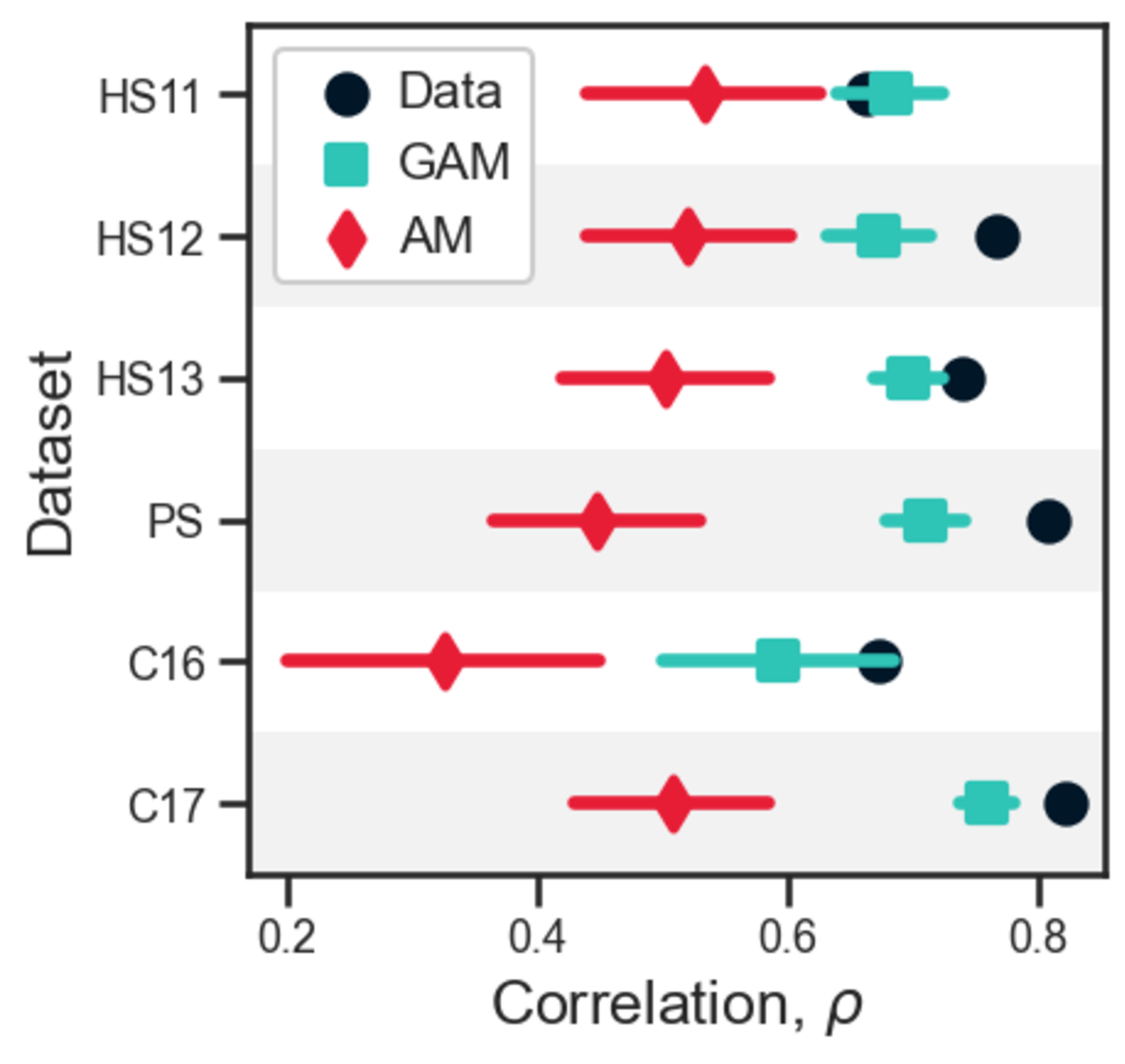
We count the unique number of groups of size two, \(k^{(2)}_i\), and three, \(k^{(3)}_i\), in which each individual \(i\) takes part at any moment within the observation time of the system, and evaluate the Pearson correlation coefficient, \(\rho\), between these two quantities. We then simulate 100 times the Group Attractiveness Model, using the parameters fitted from the group size distributions, and evaluate for each run the linear correlation between the groups of sizes two and three. Again, we consider the Attractiveness Model as a reference model.

The results are reported in 3, Fig. S4 and Fig. S6. We observe that, in general, face-to-face interactions in pairs and triads tend to be highly correlated in real-world systems (black circles), with \(\rho\) varying between 0.56 and 0.85. This aspect of the empirical datasets is well reproduced by the GAM (blue squares), for which the average correlation coefficient never goes below 0.54. Moreover, the GAM is able to predict the exact value of \(\rho\) for half of the systems while slightly underestimating it for the others. The AM, instead, systematically underestimates the correlations between groups of sizes two and three (red diamonds), with values consistently below 0.53, down to 0.33.

The correlation analysis highlights the relevance of considering higher-order mechanisms to describe human face-to-face interactions. In the Attractiveness Model, which is based on a dyadic approach, groups of more than two agents are constructed as a collection of pairs of agents. For example, if three agents form three pairs at a given time step, we assume them to interact in a group of three agents. Consequently, the correlation between groups of two and three agents reduces, especially in those scenarios with a high density of agents, i.e., the “C16” dataset. The lower correlation in the AM is not simply an effect of how we reconstruct groups from pairwise interactions, as in empirical systems, where groups are obtained in the same way, we observe high correlation values. This means that groups in real-world systems are not simply a collection of dyadic contacts. In fact, the Group Attractiveness Model, which naturally accounts for group interactions, correctly reproduces the high values of correlation observed in the data.

The hierarchical structure of group burstiness↩︎

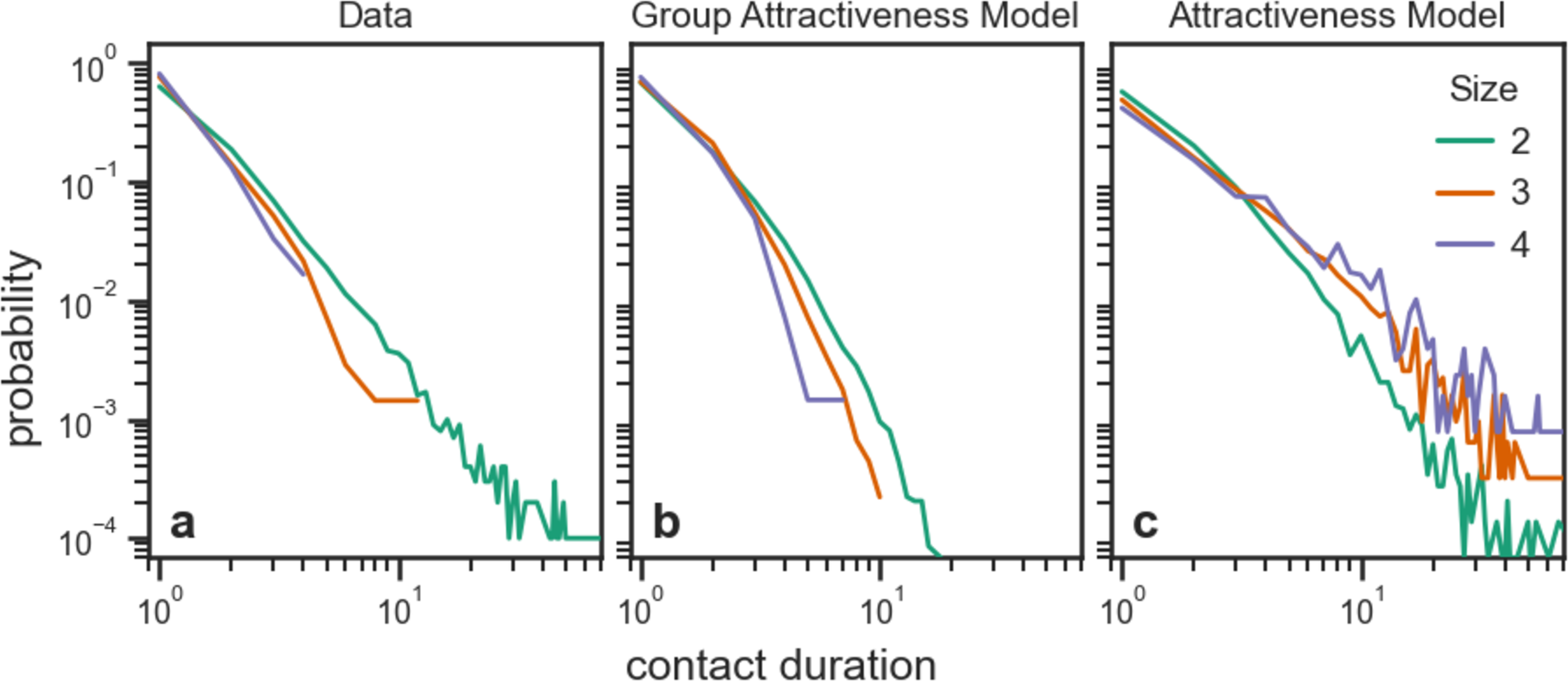
A distinctive characteristic of human face-to-face interactions is their bursty behavior [11], [54]. In particular, the duration of contacts between individuals displays broad-tailed distributions, indicating that most contacts are brief and few last for long periods of time, with no characteristic time scale. Recent literature has shown that burstiness is not limited to pairwise contacts, as group interactions show similar temporal patterns [30], [34], [55]. Interestingly, the distributions of the contact duration are typically organized in a hierarchy, with smaller groups showing broader distributions compared to larger ones, a feature that also emerges in the social systems we investigate (here we focus on the “HS11” dataset, panel a of 4; the analysis of the other datasets is reported in the Supplementary Information, Figs. S3-S11). Note that here we define the contact duration as the number of consecutive time steps for which an interaction is present.

Whereas the (individual) Attractiveness Model succeeds in reproducing the broad-tailed distribution of pairwise contacts [19], it fails to recover the hierarchical structure of group interactions. In particular, the model predicts larger groups to be more stable than smaller ones, namely that groups with more individuals remain in contact for longer (panel c of 4 and Figs. S3-S11 in Supplementary Information) [20]. This discrepancy with empirical evidence is probably due to the fact that larger groups of agents in the AM tend to be more attractive, as it is more likely that individuals with high attractiveness are members of the group.

Contrarily, capitalizing on the higher-order mechanism of group formation based on group attractiveness, the GAM is able to produce broad-tailed distributions for the contact duration as well as their hierarchical organization (panel b of 4 and Figs. S7-S18 in the Supplementary Information). Yet, we observe that the distributions are often narrower compared to the empirical ones, especially in scenarios where the density of agents is high (see results on the “C16” dataset in the Supplementary Information). This is probably due to how we define the probability that an agent interacts with its neighbors, i.e., 2 . Specifically, in a dense environment, each agent will interact with a probability that tends to the average value of the group attractiveness, meaning that individuals with high attractiveness, namely those contributing the most to the persistence of interactions, do not have a strong effect. Further studies should aim to understand the relationship between the broadness of the distributions and their hierarchical organization.

Higher-order homophily in face-to-face interactions↩︎

In many social contexts, people prefer to build ties with others whom they perceive as similar to themselves [56]. This pervasive characteristic, known as homophily, shapes the “social world” of individuals, thus profoundly influencing how behavior spreads [57], biases [58] and social norms [59] form, and segregation emerges [60], [61]. Homophily characterizes face-to-face interactions as well [12], [47], [62], driving the onset of inequalities even at such a fundamental scale [24].

While homophily is usually measured at the level of pairs of individuals, recent studies have aimed to capture it at the level of groups of three or more individuals [63]–[65]. We can use the Group Attractiveness Model to analyze higher-order homophilic patterns in face-to-face interactions. Specifically, we enrich the model by associating agents with a set of attributes and by tuning the probability that an agent interacts with its neighbors according to their attributes. Following [24], we define group formation as a two-step process that incorporates attractiveness and homophilic preferences: First, each agent decides whether to stay or to walk away based on the attractiveness of its neighborhood (see 2 ); If it stays, the agent chooses the group(s) to which it connects based on its own attributes and those of the group member(s) (panel a of 5).

To illustrate the second step, let us assume that each agent is associated with a single attribute. An agent with attribute \(\alpha\) close to an agent with attribute \(\beta\) will form a group of two with probability \(h^{(2)}_{\alpha\beta}\). Note that \(h^{(2)}_{\alpha\beta}\) represents the probability that it is the agent with attribute \(\alpha\) to start the interaction, and in general \(h^{(2)}_{\alpha\beta} \neq h^{(2)}_{\beta\alpha}\). Similarly, if the agent is close to a group of two agents having attributes \(\beta\) and \(\gamma\), respectively, it will form a group of three with probability \(h^{(3)}_{\alpha\beta\gamma}\). Therefore, the probability of forming groups of various sizes based on the agents’ attributes is determined by a set of homophily matrices, \(H^{(2)}\), \(H^{(3)}\), and so on. Here, we will focus on a single binary attribute, i.e., \(\alpha\in\{0,1\}\), using the information on gender contained in six of the datasets to test the ability of our model to reproduce higher-order mixing patterns in face-to-face interactions (from now on, attribute \(0\) will denote women, while attribute \(1\) will denote men).

To determine the elements of the homophily matrix \(H^{(2)} = [[h_{00},h_{01}],[h_{10},h_{11}]]\) (superscripts are dropped for simplicity), we evaluate the fraction of groups of size two in the different configurations, i.e., female-female, male-male, and female-male, that are formed from two individuals not previously interacting, that is \(i\) and \(j\) form a group at time \(t\) but they are not part of any common group at time \(t-1\). Such fractions can be written in terms of the elements of the homophily matrix (see Materials and Methods for details), as \[\begin{align} e_{00} = \frac{f_0^2 (1-h_{01}^2)}{f_0^2 (1-h_{01}^2) + 2f_0f_1 (1-h_{00}h_{11}) + f_1^2 (1-h_{10}^2)}, \nonumber \\ e_{01} = \frac{2f_0f_1 (1-h_{00}h_{11})}{f_0^2 (1-h_{01}^2) + 2f_0f_1 (1-h_{00}h_{11}) + f_1^2 (1-h_{10}^2)}, \\ e_{11} = \frac{f_1^2 (1-h_{10}^2)}{f_0^2 (1-h_{01}^2) + 2f_0f_1 (1-h_{00}h_{11}) + f_1^2 (1-h_{10}^2)}, \nonumber \end{align}\] where \(e_{00}\), \(e_{01}\), and \(e_{11}\), denotes the fractions of groups formed by two women, a woman and a man, and two men, respectively, while \(f_0\) and \(f_1 = 1-f_0\) represent the fraction of women and men. To estimate the elements of the homophily matrix \(H^{(3)} = [[h_{000},h_{001},h_{011}],[h_{100},h_{101},h_{111}]]\), we count the groups of size three in the different configurations that are formed by aggregation of an individual in a group of size two, i.e., at time \(t-1\) two individuals \(i\) and \(j\) form a group, at time \(t\) an individual \(k\), not previously interacting with them, joins the group. In other words, we count the transitions of dyads to triads driven by the addition of one member. Based on the gender of the individuals joining the group, we have two sets of transitions. A woman can join a group of two other women, two men, or a woman and a man. The fraction of these transitions can be written in terms of the first row of the homophily matrix \(H^{(3)}\) (see Materials and Methods), namely \[\begin{align} \tau_{0\rightarrow (0,0)} = \frac{\varepsilon_{00}h_{000}}{\varepsilon_{00}h_{000} + \varepsilon_{01}h_{001} + \varepsilon_{11}h_{011}}, \nonumber \\ \tau_{0\rightarrow (0,1)} = \frac{\varepsilon_{01}h_{001}}{\varepsilon_{00}h_{000} + \varepsilon_{01}h_{001} + \varepsilon_{11}h_{011}}, \\ \tau_{0\rightarrow (1,1)} = \frac{\varepsilon_{11}h_{011}}{\varepsilon_{00}h_{000} + \varepsilon_{01}h_{001} + \varepsilon_{11}h_{011}}, \nonumber \end{align}\] where \(\tau_{0\rightarrow (\alpha,\beta)}\) indicates the fractions of transitions, while \(\varepsilon_{\alpha\beta}\) denotes the fractions of unique groups of size two in the various configurations. Note that \(e_{\alpha\beta}\) indicates dyads emerging at a given time from two not previously interacting individuals; instead, \(\varepsilon_{\alpha\beta}\) denotes dyads that are active at a given time, including those formed in previous time steps that persisted over time, and those generated from other dynamics, e.g., a group of three that loses a member. In the same way, men can join groups of two individuals in different configurations, the fraction of which can be expressed in terms of the second row of the homophily matrix \(H^{(3)}\), namely \[\begin{align} \tau_{1\rightarrow (0,0)} = \frac{\varepsilon_{00}h_{100}}{\varepsilon_{00}h_{100} + \varepsilon_{01}h_{101} + \varepsilon_{11}h_{111}}, \nonumber \\ \tau_{1\rightarrow (0,1)} = \frac{\varepsilon_{01}h_{101}}{\varepsilon_{00}h_{100} + \varepsilon_{01}h_{101} + \varepsilon_{11}h_{111}}, \nonumber \\ \tau_{1\rightarrow (1,1)} = \frac{\varepsilon_{11}h_{111}}{\varepsilon_{00}h_{100} + \varepsilon_{01}h_{101} + \varepsilon_{11}h_{111}}. \end{align}\] A similar approach can be adopted to evaluate the matrices modulating the formation of groups of four or more individuals (see Methods). As larger groups are less abundant, for simplicity, we here limit our analysis to groups of size two and three.

Panels b and c of 5 display the homophily matrices \(H^{(2)}\) and \(H^{(3)}\) obtained for the interactions in the “HS11” dataset (see Supplementary Information for the analysis of the other five systems). At the level of pairwise interactions, we observe that women do not have a clear homophilic behavior, as they interact with other women and men with almost the same probability. Conversely, men are strongly homophilic, as the model predicts a substantial difference between the interaction probabilities. Remarkably, things change in groups of size three. In this case, women tend to be more homophilic, while men do not have a strong gender preference when joining groups of two individuals. Homophilic preferences depend on the group size in a nontrivial way: Here we observe discordant behavior, i.e., men tend to be homophilic in pairs, whereas women in triples, while other social systems can display a consistent pattern (see Panels a and b of Figs. S19-S23 in Supplementary Information).

Finally, we test the capability of the GAM to reproduce mixing patterns in social systems. Panel d of 5 shows the fraction of unique groups of size three in the different gender configurations present in the data (black bars), together with those predicted by the GAM (blue bars). For comparison, we consider the Social-Attractiveness Model (SAM) proposed in [24] (yellow bars). Similarly to our model, in the SAM a population of mobile agents performs a random walk interacting with the others based on the intrinsic attractiveness of individuals and their attributes, i.e., gender. Yet, this model only accounts for pairwise interactions, so mixing patterns at the level of groups of three agents are ultimately determined by homophily at the level of pairs. Note again that the fraction of unique triads formed over time differs from the fraction of triads generated at a given time step as a result of an agent joining a dyad, i.e., \(\tau_{0\rightarrow (\alpha,\beta)}\). Our results show that considering higher-order homophily better reproduces the gender configurations in the data. Particularly, we observe that the SAM overestimates the tendency of men to interact with their same gender, generating too many groups with three men or two men and a woman. Conversely, our model provides significantly better predictions of the empirical mixing patterns (the better performance of GAM is consistent across different datasets; see Panels c of Figs. S19-S23 in Supplementary Information). Still, we observe some mismatch, particularly in the fraction of groups with three women. This might have several explanations, including differences in individual behavior or in the frequency of contacts between the two genders [62], as well as other mechanisms of group formation/dissolution that the Group Attractiveness Model does not account for [30], [33], [34]. Overall, our results shed light on how higher-order effects can influence mixing patterns in social systems, underlining the importance of measuring homophily at the level of groups.

Discussion↩︎

Humans are social animals that communicate, gather, and live in groups. Even a fundamental level of social interactions, such as face-to-face contacts, is characterized by groups of various sizes. Although models based on dyadic representations, i.e., complex networks, have proved to be a valuable tool to characterize different properties of face-to-face interactions, they fall short when it comes to replicating structural and temporal features of groups. This is crucial, as group interactions can dramatically change the collective behavior of complex social systems, leading to super-exponential disease spreading [66], triggering critical mass effects in social contagion [67], [68], and boosting the ability of committed minorities [69] to overturn social norms [70].

In this paper, we presented the Group Attractiveness Model, an agent-based model that accounts for the dynamics of groups of individuals interacting face-to-face. Our model is able to reproduce many aspects of real-world systems, including the distribution of groups, the correlation in their number, their persistence in time, and the presence of mixing patterns. Remarkably, the GAM captures characteristics of group conversations in a variety of social contexts, from conferences and exhibitions, where interactions can often be spontaneous, to households in a village, where relationships among group members are more personal and intimate. The superior performance of the GAM compared to pairwise methods marks the need to adopt higher-order models to investigate groups in face-to-face interactions.

Despite its capability to replicate different features of group interactions, others remain beyond reach. For instance, our model is Markovian, as agents decide whether to interact with others without memory of the previous time steps. Face-to-face interactions, instead, are characterized by complex memory effects, with each group having memory of itself and others [33]. The asymmetric nature of memory can determine preferred temporal directions in group formation and dispersal that cannot be described by our model, as both dynamics are governed by the same mechanism, i.e., group attractiveness. Moreover, while smaller groups tend to evolve gradually, with one or few members at the time joining/leaving the group, larger groups can have more complex dynamics [30], [33], [34] that the Group Attractiveness Model does not take into account.

In empirical systems, the distributions of group duration are broad-tailed, and, in general, smaller groups have broader distributions than larger ones, i.e., smaller groups last longer. Although our model reproduces this feature, we observed that denser environments lead to narrower contact duration distributions, likely due to larger volumes of group aggregation and disaggregation. However, as tuning the density allows us to correctly predict the number of groups of different sizes, a trade-off between the group statistics and their temporal duration remains. In addition, the data do not provide spatial information about the environment in which contacts take place, making it difficult to determine the appropriate value of agent density. Further modeling efforts should thus aim at investigating how the spatial dimension, the number of groups, the profile and hierarchical organization of the duration distributions relate to one another.

Our modeling framework builds on several simplifications. First, it assumes that different stages of group dynamics, i.e., joining pre-existing groups, remaining in them, and leaving them, are governed by a single mechanism, namely the choice of agents to interact or walk away based on the average attractiveness of the groups around them. In principle, these processes could be i) governed by different group properties, or ii) regulated by the same quantity, e.g., the group attractiveness, in distinct ways. Second, attractiveness is here an inherent feature of conversational groups, as determined by the attractiveness of the individuals forming them. However, it is reasonable to think that the same group can attract agents in different ways based on their individual characteristics. While the extension of our model to include gender relates to this aspect, we believe that further studies in this direction are necessary. In connection to this, our model does not distinguish for the types of social groups [71] and contexts, which naturally determine the dynamics of conversations, and the structure of social networks in general [72]. Finally, the definition of the group attractiveness is not unique, as other choices are possible. The advantage of the definition in 1 is twofold: First, it captures, from a qualitative point of view, the experimental evidence that larger groups are on average less attractive and less stable than smaller ones. Second, it is parsimonious, meaning that it does not require additional parameters rather than the size of a group and the attractiveness of its members. We believe analyzing other definitions of group attractiveness that align with these principles represents a valuable direction for further work.

Similar to [19], [20], [24], the GAM allows for group overlap, namely a situation where face-to-face groups can share some of their members at a given time. This feature can be unrealistic in most social context and has the potential to affect the behavior of the model. While we verified that the GAM has, in practice, a low level of overlap that is unlikely to affect our findings (see Fig. S24), this analysis demands for further investigation into group overlap, given the role that this has on different dynamical processes [73], [74].

Though there have been a few attempts to give a higher-order definition of homophily recently [63]–[65], our understanding of homophily at the group level remains limited. Our results advance this line of research by shifting the perspective on how to measure homophily in group interactions. Instead of quantifying it a posteriori, namely based on mixing patterns in the data, we adopted an a priori approach, modeling how microscopic interactions are driven by homophilic preferences. Yet our model also comes with a few limitations. First, the GAM is currently limited to a single binary attribute, and further work could aim at extending it to multiple and non-binary attributes. While the non-binary attribute generalization is straightforward, the multi-attribute case requires more attention. On the one hand, one could consider a set of matrices for each attribute associated with the agents and thus define a decision-making process over these multiple matrices. Alternatively, one could adopt an intersectional approach, defining a single set of matrices that modulates the probability of agents to interact based on combinations of attributes, e.g., black-woman, white-man. Second, we assumed that agents differ only in terms of their intention to interact with their close neighbors, while other factors can be at play, both at an individual and at an attribute level (e.g., one can assume that agent attractiveness correlates with their attributes). Therefore, one has to be aware that our findings on homophily holds valid under this assumption on the behavior. Further generalizations of the model including multiple attributes or alternative behavioral processes could provide a robustness check on our findings. More in general, given the prominence that both group interactions and homophily have (separately) in social systems, a deeper understanding of higher-order homophily is essential.

Beyond ABMs, statistical approaches like the Relational HyperEvent Model (RHEM) [75], [76] can provide insights on how higher-order contacts depend on group characteristics. Their focus is on measuring how specific covariates, depending on the characteristics of the members of a group and their previous interactions, affect the group interaction rate. These empirical methods can serve as a natural complement to our theoretical model: While our approach allows us to study whether specific mechanisms (e.g., the group attractiveness) are sufficient to produce observed patterns and generate synthetic data, they enable hypothesis testing on what mechanisms drive group interactions.

Overall, our work contributes to the study of human face-to-face interactions through the lens of group dynamics and higher-order mechanisms. Given its ability to reproduce different features of the data, we are confident that our model will prove to be beneficial in investigating how groups affect different phenomena, including social contagion, epidemic spreading, and the emergence of mixing patterns and segregation in networked populations.

Methods↩︎

Reconstructing groups from face-to-face pairwise data↩︎

To assess the features of the Group Attractiveness Model, we use datasets from the SocioPatterns collaboration [11]. These datasets store face-to-face interactions as a list of dyadic contacts with a resolution of 20 seconds. Therefore, they do not provide any information on group interactions, i.e., face-to-face conversations involving two or more individuals, in the social systems. However, given the fine-grained temporal resolution of the data, we are able to reconstruct groups of more than two individuals. Specifically, if at time \(t\) in the dataset there are all possible dyadic contacts among \(s\) individuals, we can reasonably assume that they are interacting together in a group. For example, if at time \(t\) an individual \(i\) is in contact with individuals \(j\) and \(k\), and these two are also interacting, we can safely say that \(i\), \(j\) and \(k\) form a group of three individuals.

Fitting the homophily matrices↩︎

The Group Attractiveness Model can be extended to assess higher-order mixing patterns in face-to-face interactions. Specifically, we can enrich the model by tuning the probability that an agent interacts with a neighboring group based on their attributes. These probabilities are determined by a set of homophily matrices, \(H^{(2)}\), \(H^{(3)}\), and so on, one for each group size. Here, we show how we can analytically derive the homophily matrices in the case of a single, binary attribute \(\alpha\in\{0,1\}\). Since larger groups are less abundant in the data, we focus on groups of size two and three, tuned by the matrices \(H^{(2)} = [[h_{00}, h_{01}],[h_{10},h_{11}]]\) and \(H^{(3)} = [[h_{000}, h_{001}, h_{011}],[h_{100},h_{101},h_{111}]]\) (the superscripts are omitted for simplicity). \(h_{\alpha\beta}\) denotes the probability that an agent with attribute \(\alpha\) starts to interact with an agent having attribute \(\beta\), while \(h_{\alpha\beta\gamma}\) represents the probability that an agent with attribute \(\alpha\) starts to interact with a group of two agents having attributes \(\beta\) and \(\gamma\), respectively.

Groups of two agents can be in three different configurations, namely \((0,0)\), \((0,1)\), and \((1,1)\). Let us consider the scenario in which two agents that are not interacting, i.e., they are not part of any common group, get in contact and form a group. We denote the number of pairs in each configuration generated at time \(t\) as \(E_{00}\), \(E_{01}\), and \(E_{11}\), respectively. In general, we can write the number of pairs in configuration \((\alpha,\beta)\) as \[E_{\alpha\beta} = G^{(2)}p_{ij,\alpha\beta}.\] \(G^{(2)}\) denotes the average number of interactions between two agents (previously not interacting) that could be formed without considering homophily. \(G^{(2)}\) depends on number of agents \(N\), their radius of action \(d\), the size of the environment \(L\), and the attractiveness distribution. \(p_{ij,\alpha\beta}\) represents the probability that two agents \(i\) and \(j\) (i) have attributes \(\alpha\) and \(\beta\), respectively, and (ii) start interacting according to their attributes. A pair is created in three different situations, depending on whether (1) only \(i\), (2) only \(j\), or (3) both \(i\) and \(j\) initiate the formation of the group. Therefore, we can write \(p_{ij,\alpha\beta}\) as \[p_{ij,\alpha\beta} = p_{i\rightarrow j,\alpha\beta} + p_{i\leftarrow j,\alpha\beta} + p_{i\leftrightarrow j,\alpha\beta},\] where the arrows indicate the three possible scenarios of group formation. In the case of two agents with attributes \(\alpha=\beta=0\), we have \[\begin{align} p_{ij,00} &&= p_{i\rightarrow j,00} + p_{i\leftarrow j,00} + p_{i\leftrightarrow j,00} \nonumber\\ &&=f_0^2 \times h_{00}(1-h_{00}) + f_0^2 \times (1-h_{00})h_{00} + f_0^2 \times h_{00}^2 \nonumber\\ &&= f_0^2(1-h_{01}^2), \end{align}\] where \(f_0\) is the fraction of agents with attribute 0, and we assumed \(h_{00} + h_{01} =1\) [24]. Hence, the number of pairs in state \((0,0)\) generated at time \(t\) is \[E_{00} = G^{(2)}f_0^2 (1-h_{01}^2).\] Similarly, we can write the number of groups in state \((1,1)\) as \[E_{11} = G^{(2)}f_1^2 (1-h_{10}^2),\] where \(f_1\) is the fraction of agents with attribute 1, and we assumed \(h_{10} + h_{11} =1\). Finally, the number of groups in state \((0,1)\) is given by \[E_{01} = 2 G^{(2)}f_0f_1 (1-h_{00}h_{11}),\] where the factor two comes from the fact that \(i\) and \(j\) can have either attributes 0 or 1. We can then normalize the number of groups in each configuration by the total number of groups generated, obtaining the fractions \[\begin{align} e_{00} = \frac{f_0^2 (1-h_{01}^2)}{f_0^2 (1-h_{01}^2) + 2f_0f_1 (1-h_{00}h_{11}) + f_1^2 (1-h_{10}^2)}, \nonumber \\ e_{01} = \frac{2f_0f_1 (1-h_{00}h_{11})}{f_0^2 (1-h_{01}^2) + 2f_0f_1 (1-h_{00}h_{11}) + f_1^2 (1-h_{10}^2)}, \nonumber \\ e_{11} = \frac{f_1^2 (1-h_{10}^2)}{f_0^2 (1-h_{01}^2) + 2f_0f_1 (1-h_{00}h_{11}) + f_1^2 (1-h_{10}^2)}. \label{eq:fractions95two} \end{align}\tag{3}\] In the case of gender homophily, setting \(f_0\) and \(f_1\) equal to the fraction of female and male individuals, and \(e_{\alpha\beta}\) equal to the average fractions of pairs formed at time \(t\), where the individuals were not interacting at time \(t-1\), we can estimate the entries of \(H^{(2)}\).

If \(h_{\alpha\alpha} > 1/2\), agents prefer to interact with those having the same attribute, namely, the system is in a homophilic regime. Instead, when \(h_{\alpha\alpha} < 1/2\) agents tend to interact more with those having the other attribute, i.e., heterophilic regime. The case \(h_{\alpha\alpha} = 1/2\) corresponds to the neutral scenario where agents interact without any preferences.

We now consider the scenario in which an agent with attribute \(\alpha\) joins a pair of interacting agents that are within its scope. We denote the number of groups of size three in configuration \((\alpha,\beta,\gamma)\) generated as \(T_{\alpha\rightarrow(\beta,\gamma)}\). This can be written as \[T_{\alpha\rightarrow (\beta,\gamma)} = M^{(2)}\varepsilon_{\beta\gamma}h_{\alpha\beta\gamma},\] where \(M^{(2)}\) is the average number of groups of size two within the scope of an agent, \(\varepsilon_{\beta\gamma}\) is the fraction of groups in state \((\beta,\gamma)\), while \(h_{\alpha\beta\gamma}\) is the element of the homophily matrix \(H^{(3)}\) denoting the probability that an agent with attribute \(\alpha\) interacts with a pairs of agents with attributes \(\beta\) and \(\gamma\), respectively. Note that \(e_{\beta\gamma}\) denotes the fraction of dyads in state \((\beta,\gamma)\) formed at a given time, and differs from \(\varepsilon_{\beta\gamma}\), which is the fraction of dyads active at a given time. This also includes the dyads formed previously that persisted over time, and those generated from other dynamics, e.g., a group of three that loses a member. Focusing on \(\alpha=0\), we can write the number of groups of size three formed at time \(t\) as \[\begin{align} T_{0\rightarrow (0,0)} = M^{(2)}\varepsilon_{00}h_{000}, \nonumber \\ T_{0\rightarrow (0,1)} = M^{(2)}\varepsilon_{01}h_{001}, \nonumber \\ T_{0\rightarrow (1,1)} = M^{(2)}\varepsilon_{11}h_{011}. \end{align}\] Normalizing by the total number of groups generated, we obtain the fractions \[\begin{align} \tau_{0\rightarrow (0,0)} = \frac{\varepsilon_{00}h_{000}}{\varepsilon_{00}h_{000} + \varepsilon_{01}h_{001} + \varepsilon_{11}h_{011}}, \nonumber \\ \tau_{0\rightarrow (0,1)} = \frac{\varepsilon_{01}h_{001}}{\varepsilon_{00}h_{000} + \varepsilon_{01}h_{001} + \varepsilon_{11}h_{011}}, \nonumber \\ \tau_{0\rightarrow (1,1)} = \frac{\varepsilon_{11}h_{011}}{\varepsilon_{00}h_{000} + \varepsilon_{01}h_{001} + \varepsilon_{11}h_{011}}. \label{eq:fractions95three950} \end{align}\tag{4}\] Similarly, for an agent with attribute 1, we find \[\begin{align} \tau_{1\rightarrow (0,0)} = \frac{\varepsilon_{00}h_{100}}{\varepsilon_{00}h_{100} + \varepsilon_{01}h_{101} + \varepsilon_{11}h_{111}}, \nonumber \\ \tau_{1\rightarrow (0,1)} = \frac{\varepsilon_{01}h_{101}}{\varepsilon_{00}h_{100} + \varepsilon_{01}h_{101} + \varepsilon_{11}h_{111}}, \nonumber \\ \tau_{1\rightarrow (1,1)} = \frac{\varepsilon_{11}h_{111}}{\varepsilon_{00}h_{100} + \varepsilon_{01}h_{101} + \varepsilon_{11}h_{111}}. \label{eq:fractions95three951} \end{align}\tag{5}\] Assuming that \(h_{000} + h_{001} + h_{011} = h_{100} + h_{101} + h_{111} = 1\), we can estimate the entries of the homophily matrix \(H^{(3)}\). Specifically, we set \(\varepsilon_{\beta\gamma}\) equal to the fractions of unique groups of size two in the different gender configurations, while \(\tau_{\alpha\rightarrow (\beta,\gamma)}\) can be evaluated by counting how many times in the data a pair of interacting individuals at time \(t-1\) is followed by a group of size three at time \(t\). Note that the neutral scenario with no homophilic preferences in the group formation corresponds to \(h_{000} = h_{011} = 1/3\) and \(h_{100} = h_{111} = 1/3\).

Finally, we can recover the Group Attractiveness Model without homophily by assuming that all agents have the same attribute, say \(f_0 = 1\), and that the corresponding homophilic interaction probabilities are equal to 1, namely \(h_{00} = 1\) (no matter the value of \(h_{11}\)) and \(h_{000} = 1\) (no matter the values of \(h_{100}\) and \(h_{111}\)).

We can estimate the other homophily matrices following the same derivation applied to \(H^{(3)}\). To derive \(H^{(d)}\), one needs to estimate \(2d\) elements from \(2d\) equations describing how agents join groups of size \(d-1\), together with 2 constraints on the row sum of the matrix. Formally, one has to solve the system of equations \[\begin{align} &\tau_{\nu\rightarrow \sigma^{(d-1)}} = \frac{f\left(\sigma^{(d-1)}\right)h_{\nu\sigma^{(d-1)}}}{\sum\limits_{\sigma^{(d-1)}}{f\left(\sigma^{(d-1)}\right)h_{\nu\sigma_{d-1}}}} \\ & \sum\limits_{\sigma^{(d-1)}}h_{\nu\sigma^{(d-1)}} = 1 \end{align},\] where \(\nu\in[0,1]\), \(\sigma^{(d-1)}\) is one of the \(d\) possible states for groups of size \(d-1\), \(\tau_{\nu\rightarrow \sigma^{(d-1)}}\) is the fraction of transitions in which agents with attribute \(\nu\) join groups in state \(\sigma^{(d-1)}\), \(f(\sigma^{(d-1)})\) is the fraction of groups of size \(d-1\) in state \(\sigma^{(d-1)}\), while \(h_{\nu\sigma^{(d-1)}}\) is an element of the homophily matrix \(H^{(d)}\). Note that each element of \(H^{(d)}\) has \(d\) indices, one being \(\nu\), and the other \(d-1\) coming from \(\sigma^{(d-1)}\). As done for \(d=3\) with \(\tau_{\nu\rightarrow (\beta,\gamma)}\) and \(\varepsilon_{\beta\gamma}\), one can estimate \(\tau_{\nu\rightarrow \sigma^{(d-1)}}\) and \(f(\sigma^{(d-1)})\) from the data, to finally derive \(H^{(d)}\).

Data Availability↩︎

Data on contacts in scientific conferences are available upon request at https://doi.org/10.7802/235. All other datasets are freely available at https://www.sociopatterns.org/datasets.

Code Availability↩︎

A Python implementation of the Group Attractiveness Model is available as part of the HGX library [77].

Acknowledgments↩︎

L.G. thanks Rahel Geppert and Rebeka O. Szabo for the insightful suggestions and discussion. L.G. acknowledges support from the Villum Foundation (project no. 57396) at the University of Copenhagen. L.G. and F.B. acknowledge support of the Air Force Office of Scientific Research under award number FA8655-22-1-7025. C.Z. acknowledges funding by the European Union under Horizon EU project LearnData, 101086712. C.Z. acknowledges support from the Villum Foundation (project no. 37394) at the University of Copenhagen.

References↩︎