1 Introduction↩︎

Least squares linear regression and \(\ell_p\) linear regression are some of the most fundamental and practically valuable computational problems in statistics and optimization. In this problem, our input is an \(n\times d\) matrix \(\bfA\in\mathbb{R}^{n\times d}\) and a response vector \(\bfb\in\mathbb{R}^n\), and our goal is to output an approximate minimizer \(\hat{\bfx}\in\mathbb{R}^d\) such that \[\label{eq:lp-regression} \norm{\bfA\hat{\bfx}-\bfb}_p^p \leq (1+\eps)\min_{\bfx\in\mathbb{R}^d}\norm{\bfA\bfx-\bfb}_p^p.\tag{1}\] Among the vast literature on \(\ell_p\) regression, sampling algorithms and coresets, which are algorithms that select a weighted subset of the rows of \(\bfA\) and \(\bfb\) that suffice to solve \(\ell_p\) regression, have played major roles in the development of efficient algorithms. That is, we seek a diagonal matrix \(\bfS\in\mathbb{R}^{n\times n}\) with few non-zero entries, i.e., \(\nnz(\bfS) \ll n\), such that the weighted subset of rows \(\bfS\bfA\) and \(\bfS\bfb\) are sufficient to compute a solution \(\hat{\bfx}\) satisfying 1 . We will often refer to \(\nnz(\bfS)\) as the sample complexity. We focus on approaches that construct \(\bfS\) by i.i.d.sampling of each of the \(n\) rows:

Two well-studied guarantees for \(\bfS\) are strong coresets and weak coresets. Strong coresets refer to coresets that preserve the value of the objective function at every point in the domain, while weak coresets only guarantee that the unconstrained minimizer is preserved. If we only care about solving the unconstrained \(\ell_p\) regression problem, then weak coresets are sufficient to solve this problem, and it is known that weak coresets can be substantially smaller than strong coresets in certain settings [1]. On the other hand, strong coresets are necessary when the objective function must be evaluated at points away from the optimum, for example for constrained optimization problems.

The efficient construction of coresets for \(\ell_p\) regression has been studied in a long line of work [2]–[5] culminating in the \(\ell_p\) Lewis weight sampling algorithm [6]–[13], which gives an algorithm that constructs a strong coreset \(\bfS\) with \[\nnz(\bfS) = \begin{cases} \tilde{O}(\eps^{-2}d) & p \leq 2 \\ \tilde{O}(\eps^{-2}d^{p/2}) & p > 2 \end{cases}.\] A related line of work in the active \(\ell_p\) regression setting shows that weak coresets for \(\ell_p\) regression with \[\nnz(\bfS) = \begin{cases} \tilde{O}(\eps^{-2}d) & p = 1 \\ \tilde{O}(\eps^{-1}d) & 1 < p < 2 \\ O(\eps^{-1}d) & p = 2 \\ \tilde{O}(\eps^{-(p-1)}d^{p/2}) & p > 2 \end{cases}\] can be constructed even without knowing \(\bfb\) [1], [14]–[17]. Note that these bounds strictly improve over the strong coreset guarantees of \(\ell_p\) Lewis weight sampling for \(1 < p < 3\).

1.1 Multiple \(\ell_p\) regression↩︎

It is often the case that we are interested in more than just one target \(\bfb\) to predict, and in general, we may wish to simultaneously fit \(m\) target vectors that are given by a matrix \(\bfB\in\mathbb{R}^{n\times m}\) and solve the minimization problem \[\min_{\bfX\in\mathbb{R}^{d\times m}}\norm*{\bfA\bfX - \bfB}_{p,p}^p = \min_{\bfX\in\mathbb{R}^{d\times m}}\sum_{j=1}^m \norm*{\bfA\bfX\bfe_j - \bfB\bfe_j}_p^p\] This is known as the multiple response \(\ell_p\) regression problem, or simply the multiple \(\ell_p\) regression problem, and is the focus of the present work.

1.1.1 Coreset constructions for \(p=2\)↩︎

For \(p = 2\), the construction of strong coresets for the multiple response problem follows almost immediately from strong coresets for the single response problem due to orthogonality and the Pythagorean theorem, and we can construct \(\bfS\) such that \[\norm{\bfS(\bfA\bfX-\bfB)}_F^2 = (1\pm\eps)\norm{\bfA\bfX-\bfB}_F^2\] with \(\nnz(\bfS) = \tilde{O}(\eps^{-2}d)\) samples. Indeed, assume without loss of generality that \(\bfA\) has orthogonal columns, and suppose that \(\bfS\) satisfies

• \(\norm{\bfS\bfA\bfx}_2^2 = (1\pm\eps)\norm{\bfA\bfx}_2^2\) for every \(\bfx\in\mathbb{R}^d\) (i.e., \(\bfS\) is a subspace embedding)

• \(\norm{\bfS(\bfA\bfX^*-\bfB)}_F^2 = (1\pm\eps)\norm{\bfA\bfX^*-\bfB}_F^2\) where \(\bfX^*\) is the optimal minimizer

• \(\norm{\bfA^\top\bfS^\top\bfS(\bfA\bfX^*-\bfB)}_F^2 \leq (\eps^2/d)\norm{\bfA}_F^2\norm{\bfA\bfX^*-\bfB}_F^2 = \eps^2\norm{\bfA\bfX^*-\bfB}_F^2\)

Then, the following argument of Section 7.5 of [18] shows that \(\bfS\) is a strong coreset. Indeed, \[\begin{align} \norm{\bfS(\bfA\bfX-\bfB)}_F^2 &= \norm{\bfS\bfA(\bfX-\bfX^*)}_F^2 + \norm{\bfS(\bfA\bfX^*-\bfB)}_F^2 + 2\tr\parens*{(\bfX-\bfX^*)^\top\bfA^\top\bfS^\top\bfS(\bfA\bfX^*-\bfB)} \end{align}\] by expanding the square, and the inner product term is bounded by \[\begin{align} \abs*{\tr\parens*{(\bfX-\bfX^*)^\top\bfA^\top\bfS^\top\bfS(\bfA\bfX^*-\bfB)}} &\leq \norm{\bfX-\bfX^*}_F\norm{\bfA^\top\bfS^\top\bfS(\bfA\bfX^*-\bfB)}_F \\ &\leq \eps\norm{\bfA(\bfX-\bfX^*)}_F\norm{\bfA\bfX^*-\bfB}_F \\ &\leq\eps\norm{\bfA\bfX-\bfB}_F^2 \end{align}\] and \(\bfS\) also preserves the quantities \(\norm{\bfS\bfA(\bfX-\bfX^*)}_F^2\) and \(\norm{\bfS(\bfA\bfX^*-\bfB)}_F^2\) up to \((1\pm\eps)\) relative error. A similar trick is available in the weak coreset setting (see, e.g., Section 3.1 of [19]), which gives a bound of \(\nnz(\bfS) = \tilde{O}(\eps^{-1}d)\) for this guarantee. Unfortunately, almost every step in the above argument uses special properties of the \(\ell_2\) norm that are not available for the \(\ell_p\) norm, and thus we will need completely different arguments to handle \(p\neq 2\).

1.1.2 Challenges for \(p\neq 2\)↩︎

If we desire only weak coresets, then prior results on active \(\ell_p\) regression in fact almost immediately provide a solution. These results show that a weak coreset \(\bfS\) for the single response \(\ell_p\) regression problem can be constructed independently of \(\bfb\), and with the dependence of \(\nnz(\bfS)\) on the failure probability \(\delta\) being polylogarithmic. Thus by setting the failure rate to \(\delta = 1/10m\), we can simultaneously solve every column of \(\bfB\) independently with overall probability at least \(9/10\).

For strong coresets, however, such a column-wise strategy must be implemented carefully. If we consider constructing a strong coreset for a single column \(j\in[m]\), then the sampling probabilities now depend on the target vector \(\bfB\bfe_j\), so the sampling complexity would need to scale as \(m\) rather than \(\poly\log(m)\) as in the previous upper bound weak coresets. On the other hand, another natural strategy is to mimic the strategy for the \(p = 2\) case and take the sampling probabilities to only guarantee an \(\ell_p\) subspace embedding for the column space of \(\bfA\) and that \(q_i \geq \norm{\bfe_i^\top\bfB^*}_p^p / \norm{\bfB^*}_{p,p}^p\) for \(\bfB^* \mathrel{\vcenter{:}}= \bfA\bfX^*-\bfB\). This is a reasonable choice of sampling probabilities, and indeed it is not hard to see that \[\norm{\bfS(\bfA\bfX-\bfB)}_{p,p}^p = (1\pm\eps)\norm{\bfA\bfX-\bfB}_{p,p}^p\] for any fixed \(\bfX\in\mathbb{R}^{d\times m}\) with only \(\nnz(\bfS) = \tilde{O}(\eps^{-2}d)\) samples for \(p<2\) and \(\nnz(\bfS) = \tilde{O}(\eps^{-2}d^{p/2})\) samples for \(p>2\) via a Bernstein tail bound. However, it is unclear how to extend a guarantee for any single \(\bfX\in\mathbb{R}^{d\times m}\) to a guarantee simultaneously for all \(\bfX\in\mathbb{R}^{d\times m}\). Although the dependence on the failure rate \(\delta\) is logarithmic, a net argument, or even more sophisticated chaining arguments, over the possible choices of \(\bfX\in\mathbb{R}^{d\times m}\) seem to require a union bound over sets of size \(\exp(dm)\), thus again introducing a linear dependence on \(m\) in the sample complexity \(\nnz(\bfS)\). As we show, a careful blend of these two ideas will be necessary to obtain our strong coreset result.

1.2 Strong coresets for multiple \(\ell_p\) regression↩︎

Our first main result is the first construction of strong coresets for multiple \(\ell_p\) regression that is independent of \(m\).

We achieve a nearly optimal dependence on \(d\) and \(\eps\), as we show that \(\Omega(d^{p/2}/\eps^p)\) rows are necessary for strong coresets in Theorem [thm:strong-coreset-lower-bound] for \(p>2\), while it is known that \(\tilde{\Omega}(d/\eps^2)\) rows are necessary even for \(m = 1\) for \(p < 2\) [20]. We note that our upper bound shows that multiple \(\ell_p\) regression is as easy as single response \(\ell_p\) regression for \(p<2\), while our lower bound demonstrates an interesting separation between the two for \(p>2\).

1.2.1 Initial \(\log m\) bound↩︎

Our main technique is to generalize the “partition by sensitivity” technique introduced in the active \(\ell_p\) regression work of [1] and show how this can be applied to the strong coreset setting. We describe the idea for the case of \(p<2\), as the case of \(p>2\) is analogous.

In the active \(\ell_p\) regression setting, we must show that we can design sampling algorithms that preserve the objective function value, even if we do not know the target vector \(\bfb\). In this setting, one of the main observations of [1] is that even though we cannot preserve \(\norm{\bfA\bfx-\bfb}_p^p\) itself, we can actually preserve the difference \(\norm{\bfA\bfx-\bfb}_p^p - \norm{\bfb}_p^p\), if \(\norm{\bfb}_p^p = O(\mathsf{OPT}^p)\) which is without loss of generality. To see this idea, assume (without loss of generality due to [5]) that we restrict our attention to \(\norm{\bfA\bfx}_p^p = O(\mathsf{OPT}^p)\). Then, the analysis of [1] proceeds by partitioning the coordinates of \(\bfb\) into two sets, those such that \(\abs{\bfb(i)}^p\) is larger than \(\eps^{-p}\bfw_i \mathsf{OPT}^p\) and those that are smaller than this threshold, where \(\bfw_i\) is the \(i\)-th \(\ell_p\) Lewis weight of \(\bfA\). It is known that \(\bfw_i\) bounds the sensitivities of \(\bfA\), that is, \(\abs{[\bfA\bfx](i)}^p \leq \bfw_i \norm{\bfA\bfx}_p^p\) so it follows that for any \(\abs{\bfb(i)}^p \geq \eps^{-p}\bfw_i \mathsf{OPT}^p\), we have that \[\abs*{\abs{[\bfA\bfx-\bfb](i)}^p - \abs{\bfb(i)}^p} = O(\eps)\abs{\bfb(i)}^p\] for any \(\bfx\in\mathbb{R}^d\) with \(\norm{\bfA\bfx}_p^p = O(\mathsf{OPT}^p)\). On the other hand, if \(\abs{\bfb(i)}^p \leq \eps^{-p}\bfw_i \mathsf{OPT}^p\), then we have by the triangle inequality that \[\abs*{\abs{[\bfA\bfx-\bfb](i)}^p - \abs{\bfb(i)}^p} \leq O(\eps^{-p})\bfw_i \mathsf{OPT}^p.\] Thus, up to an additive \(O(\eps)(\norm{\bfS\bfb}_p^p + \norm{\bfb}_p^p)\) error, \(\abs*{\abs{[\bfA\bfx-\bfb](i)}^p - \abs{\bfb(i)}^p}\) has sensitivities which are controlled by the \(\ell_p\) Lewis weights of \(\bfA\). This allows one to show that sampling by the \(\ell_p\) Lewis weights of \(\bfA\) preserves \(\norm{\bfA\bfx-\bfb}_p^p - \norm{\bfb}_p^p\) for all \(\norm{\bfA\bfx}_p^p = O(\mathsf{OPT}^p)\).

In order to apply this idea to the strong coreset setting, we generalize the above argument to multiple scales. That is, we replace \(\mathsf{OPT}^p\) by an arbitrary scale \(R\geq \norm{\bfb}_p^p\), and show that for every \(\norm{\bfA\bfx}_p^p \leq O(R)\) that \[\begin{align} \abs*{\parens*{\norm{\bfS(\bfA\bfx-\bfb)}_p^p - \norm{\bfS\bfb}_p^p} - \parens*{\norm{\bfA\bfx-\bfb}_p^p - \norm{\bfb}_p^p}} \leq \eps (R + \norm{\bfS\bfb}_p^p) \end{align}\] Finally, we can generalize this to the following guarantee by union bounding over finitely many scales \(R\), which holds for every \(\bfx\in\mathbb{R}^d\): \[\label{eq:lewis-diff} \begin{align} \abs*{\parens*{\norm{\bfS(\bfA\bfx-\bfb)}_p^p - \norm{\bfS\bfb}_p^p} - \parens*{\norm{\bfA\bfx-\bfb}_p^p - \norm{\bfb}_p^p}} \leq \eps \parens*{\norm{\bfb}_p^p + \norm{\bfS\bfb}_p^p + \norm{\bfA\bfx}_p^p} \end{align}\tag{2}\] This guarantee is in a form that can be summed over the \(m\) columns of \(\bfB\). Thus, if a \(\log m\) dependence is admissible, then we can apply the above result with failure probability \(1/10m\), union bound over the \(m\) columns, and sum the results to obtain \[\begin{align} \left\lvert (\norm{\bfS(\bfA\bfX-\bfB)}_{p,p}^p-\norm{\bfS\bfB}_{p,p}^p) - (\norm{\bfA\bfX-\bfB}_{p,p}^p-\norm{\bfB}_{p,p}^p) \right\rvert \leq \eps\parens*{\norm{\bfB}_{p,p}^p + \norm{\bfS\bfB}_{p,p}^p + \norm{\bfA\bfX}_{p,p}^p}. \end{align}\] Now suppose that we additionally have

• \(\norm{\bfS\bfB}_{p,p}^p = (1\pm\eps)\norm{\bfB}_{p,p}^p\)

• \(\norm{\bfB}_{p,p}^p = O(\mathsf{OPT}^p)\) (which is without loss of generality by subtracting an \(O(1)\)-optimal solution)

Then, we have \[\begin{align} \norm{\bfS(\bfA\bfX-\bfB)}_{p,p}^p &= \norm{\bfA\bfX-\bfB}_{p,p}^p-\norm{\bfB}_{p,p}^p+\norm{\bfS\bfB}_{p,p}^p \pm O(\eps)\parens*{\norm{\bfB}_{p,p}^p + \norm{\bfA\bfX}_{p,p}^p} \\ &= \norm{\bfA\bfX-\bfB}_{p,p}^p\pm\eps\norm{\bfB}_{p,p}^p \pm O(\eps)\parens*{\norm{\bfB}_{p,p}^p + \norm{\bfA\bfX}_{p,p}^p} \\ &= \norm{\bfA\bfX-\bfB}_{p,p}^p \pm O(\eps) \norm{\bfA\bfX-\bfB}_{p,p}^p \end{align}\] so we indeed have a strong coreset as desired.

1.2.2 Removing the \(m\) dependence↩︎

Next, we show how to completely remove the \(m\) dependence, which requires additional ideas. When applying 2 to each of the \(m\) columns, suppose that we set the failure probability to \(\poly(\eps\delta)\) instead of \(O(1/m)\). Then, this guarantee will hold for a \(1-\poly(\eps\delta)\) fraction of “good” columns, for which we can obtain \((1\pm\eps)\) approximations. On the remaining \(\poly(\eps\delta)\) fraction of “bad” columns, note that the mass of \(\bfB\) on these columns is at most \(\poly(\eps\delta)\norm{\bfB}_{p,p}^p\) with probability \(1-\delta\) by Markov’s inequality. Then on these columns, \(\norm{\bfS(\bfA\bfX-\bfB)\bfe_j}_p\) is just \(\norm{\bfS\bfA\bfX\bfe_j}_p\) up to a small total additive error of \(\poly(\eps\delta)\norm{\bfB}_{p,p}^p\). In turn, we have that \(\norm{\bfS\bfA\bfX\bfe_j}_p = (1\pm\eps)\norm{\bfA\bfX\bfe_j}_p\) by using that \(\bfS\) is an \(\ell_p\) subspace embedding. Thus, by combining with the \((1\pm\eps)\) approximation on the rest of the “good” columns, we can still ensure that \(\norm{\bfS(\bfA\bfX-\bfB)}_{p,p} = (1\pm\eps)\norm{\bfA\bfX-\bfB}_{p,p}\).

1.3 Weak coresets for multiple \(\ell_p\) regression↩︎

In the weak coreset setting, we consider a generalized multiple \(\ell_p\) regression problem, where we are given a design matrix \(\bfA\in\mathbb{R}^{n\times d}\), an “embedding” \(\bfG\in\mathbb{R}^{t\times m}\), and a target matrix \(\bfB\in\mathbb{R}^{n\times m}\), and we wish to approximately minimize the objective function \(\norm{\bfA\bfX\bfG-\bfB}_{p,p}\).

As noted previously, for multiple \(\ell_p\) regression without an embedding (i.e., \(\bfG = \bfI_t\)) the construction of weak coresets follows relatively straightforwardly by applying active \(\ell_p\) regression results along each column. However, this strategy fails when we must additionally handle the embedding matrix \(\bfG\), as this constraint couples the columns of \(\bfA\bfX\) together. Furthermore, we argue that handling the embedding \(\bfG\) is substantially more interesting that the unconstrained case. Indeed, as we see later in Sections 1.4 and 1.5, the incorporation of the embedding \(\bfG\) will allow us to handle interesting extensions of our results to settings beyond the entrywise \(\ell_p\) norm via the use of a linear embedding into this norm. We will denote the optimal value as \[\mathsf{OPT}\mathrel{\vcenter{:}}= \min_{\bfX\in\mathbb{R}^{d\times t}} \norm{\bfA\bfX\bfG-\bfB}_{p,p}\] and let \(\bfX^*\) denote the matrix achieving this optimum unless otherwise noted. We will prove the following result:

We achieve a nearly optimal dependence on \(d\) and \(\eps\), as we show that \(\Omega(d^{p/2}/\eps^{p-1})\) rows are necessary for weak coresets in Theorem [thm:weak-coreset-lower-bound] for \(p>2\). Our weak coreset upper bound result together with our strong coreset lower bound of Theorem [thm:strong-coreset-lower-bound] shows a tight \(\eps\) factor separation between the two coreset guarantees.

Note that in the statement of Theorem [thm:weak-coreset-informal], the dependence on the failure rate \(\delta\) is polynomial. This is in fact necessary if we restrict our algorithm to be of the form of “sample-and-solve” algorithms whose sampling matrices \(\bfS\) do not depend on \(\bfB\), as demonstrated in a lower bound result of Theorem 12.8 of [1]. The only reason why this dependence becomes necessary in the analysis of the upper bound is that \(\norm{\bfS(\bfA\bfX^*\bfG-\bfB)}_{p,p}^p\) may be as large as \(O\parens*{\frac{1}{\delta}}\norm{\bfA\bfX^*\bfG-\bfB}_{p,p}^p\) with probability at least \(\delta\), and this is the source of the hardness result of Theorem 12.8 of [1] as well. This is a mild problem and can be easily circumvented in one of two ways. The first is to simply allow the algorithm to incorporate the row norms of \(\bfB\) into the sampling probabilities just as in Theorem [thm:strong-coreset-informal]. However, this would not give an active regression algorithm that makes only polylogarithmic in \(\delta\) many queries. If we wish for such an active regression algorithm, then we can follow [1] and consider the following two-stage procedure. First, we can obtain a constant factor solution \(\hat{\bfX}\) with a polylogarithmic dependence on \(\delta\) by employing a “median”-like procedure (see Section 3.1 of [1]). Then, we can run \(\log\frac{1}{\delta}\) copies of the algorithm, each of which succeeds with probability \(1-\delta\). Then, we can sort the runs by their estimates \(\norm{\bfS(\bfA\hat{\bfX}\bfG-\bfB)}_{p,p}^p\) and discard half of the runs with the highest values of \(\norm{\bfS(\bfA\hat{\bfX}\bfG-\bfB)}_{p,p}^p\). This guarantees that the remaining runs have \(\norm{\bfS(\bfA\bfX^*\bfG-\bfB)}_{p,p}^p = O(1)\norm{\bfA\bfX^*\bfG-\bfB}_{p,p}^p\) with probability at least \(1-\delta\), which is enough for the rest of the argument to go through with only a polylogarithmic dependence on \(\delta\).

1.4 Applications: sublinear algorithms for Euclidean power means↩︎

Our first application of our results on coresets for multiple \(\ell_p\) regression is on designing coresets for the Euclidean power means problem. In this problem, we are given as input a set of \(n\) points \(\{\bfb_i\}_{i=1}^n\subseteq\mathbb{R}^t\), and we wish to find a center \(\hat{\bfx}\in\mathbb{R}^t\) that minimizes the sum of the Euclidean distances to \(\hat{\bfx}\), raised to the power \(p\). That is, we seek to minimize the objective function given by \[\sum_{i=1}^n \norm{\bfx - \bfb_i}_2^p = \norm{\mathbf{1}\bfx^\top-\bfB}_{p,2}^p\] where \(\mathbf{1}\) is the \(n\times 1\) matrix of all ones, \(\bfB\in\mathbb{R}^{n\times t}\) is the matrix with \(\bfb_i\) in its \(n\) rows, and \(\norm{\cdot}_{p,2}\) is the \((p,2)\)-norm of a matrix given by the \(\ell_p\) norm of the Euclidean norm of the rows. This is a fundamental problem which generalizes the well-studied problems of the mean (\(p = 2\)), geometric median (\(p = 1\)), and minimum enclosing balls (\(p = \infty\)). Coresets and sampling algorithms for this problem were recently studied by [21], who showed that a uniform sample of \(\tilde{O}(\eps^{-(p+3)})\) points suffices to output a center \(\hat{\bfx}\in\mathbb{R}^t\) such that \[\norm{\mathbf{1}\hat{\bfx}^\top-\bfB}_{p,2}^p \leq (1+\eps)\min_{\bfx\in\mathbb{R}^t}\norm{\mathbf{1}\bfx^\top-\bfB}_{p,2}^p = (1+\eps)\mathsf{OPT}^p.\] In comparison to the upper bounds, the lower bounds given by [21] was \(\Omega(\eps^{-(p-1)})\) which is off by an \(\eps^4\) factor compared to the upper bound, which was improved to \(\Omega(\eps^{-1})\) for \(1<p<2\) by [1] and \(\Omega(\eps^{-2})\) for \(p=1\) by [15], [16].

One of the main open questions highlighted by the work of [21] is to obtain tight bounds for this problem: how many uniform samples are necessary and sufficient to output a \((1+\eps)\)-approximate solution to the Euclidean power means problem. Our main contribution is a nearly optimal algorithm which matches the lower bounds of [1], [15], [16], [21].

To apply the techniques developed in this work to the Euclidean power means problem, we need to embed the \((p,2)\)-norm into the entrywise \(\ell_p\) norm. To make this reduction, we use a classic result of Dvoretzky and Milman [22], [23], which shows that a random subspace of a normed space is approximately Euclidean. We will need the following version of this result for \(\ell_p\) norms:

Note then that if \(\bfG\) is an appropriately scaled random Gaussian matrix, then we have that \[\norm{\mathbf{1}\bfx^\top-\bfB}_{p,2}^p = (1\pm\eps)\norm{\mathbf{1}\bfx^\top\bfG-\bfB\bfG}_{p,p}^p\] by the above result. We may now note that the latter optimization problem is exactly of the form of an embedded \(\ell_p\) regression problem, and thus our weak coreset results immediately apply to this problem. In fact, handling this Dvoretzky embedding is our main motivation for studying the \(\ell_p\) regression problem with the embedding. We also note that similar reductions are possible by making use of other linear embeddings between \(\ell_p\) norms [24]–[26]. The full argument is given in Appendix 9.1.

In addition to sharpening the bound of [21] to optimality, we note that our techniques, both algorithmically and in the analysis, are simpler than the prior work of [21]. The previous algorithm required partitioning the dataset into “rings” of points with similar costs and preprocessing these rings. Furthermore, the analysis uses a specially designed chaining argument with custom net constructions that require terminal Johnson–Lindenstrauss embeddings. On the other hand, our algorithm simply runs multiple instances of a “sample-and-solve” algorithm, where the run with lowest sampled mass is kept. Furthermore, the analysis largely builds on existing net constructions for \(\ell_p\) regression, and does not need terminal embeddings. In fact, our proof for the power means problem only need \(\ell_p\) regression net constructions in \(d = 1\) dimensions due to our use of Dvoretzky’s theorem, which avoids the sophisticated constructions of [7] for large \(d\) and only needs a standard volume argument (Remark [rem:simple-net]). Our partition of sensitivity can also be thought of as a coarse notion of rings, where we only consider two classes of costs, “big” and “small”, whereas prior work requires finer a classification of points into rings of points whose costs are related up to a constant factor.

1.5 Applications: spanning coresets for \(\ell_p\) subspace approximation↩︎

As a second application of our results, we give the first construction of spanning coresets for \(\ell_p\) subspace approximation with nearly optimal size. The \(\ell_p\) subspace approximation is a popular generalization of the classic Frobenius norm low rank approximation problem, where the input is a set of \(n\) points \(\{\bfa_i\}_{i=1}^n\) in \(d\) dimensions, and we wish to compute a rank \(k\) subspace \(F\subseteq\mathbb{R}^d\) that minimizes \[\sum_{i=1}^n \norm{\bfa_i^\top(\bfI_d - \bfP_F)}_2^p\] where \(\bfP_F\) denotes the orthogonal projection matrix onto \(F\). Equivalently, we can write this as \[\min_{\rank(F) \leq k}\norm{\bfA(\bfI_d - \bfP_F)}_{p,2}^p.\]

While strong and weak coresets for this problem have attracted much attention [17], [27]–[31], our main contribution to this line of research is on a different coreset guarantee, which we call spanning coresets. Spanning coresets are subsets of the points \(\bfa_i\) which span a \((1+\eps)\)-optimal rank \(k\) subspace, and is another popular guarantee in this literature [28], [32], [33]. In addition to being an interesting object in its own right [28], the existence of small spanning coresets have found applications to constructions for strong and weak coresets for \(\ell_p\) subspace approximation [30].

Our main result is the following upper bound on the size of spanning coresets.

In particular, we improve the previous best result of \(O(\eps^{-1} k^2 \log(k/\eps))\) due to Theorem 3.1 of [28] in the \(k\) dependence for all \(1 \leq p < 4\). The proof of this result is given in Section 9.2. Furthermore, we give the first lower bounds on the size of spanning coresets by generalizing an argument of [34] for \(p = 2\), showing that spanning coresets must have size at least \(\Omega(\eps^{-1}k)\) in Theorem [thm:rank-k-lower-bound]. Together, our results settle the size of spanning coresets up to polylogarithmic factors for \(1 < p < 2\). To obtain this result, we again use Dvoretzky’s theorem to embed the problem to an embedded entrywise \(\ell_p\) norm problem, and then apply our weak coreset results.

Finally, we note that our spanning coreset lower bound implies other interesting lower bounds for coresets. First, we note that weak coresets for \(\ell_p\) subspace approximation are automatically spanning coresets, so our lower bound for spanning coresets also gives the first nontrivial lower bound on the size of weak coresets for \(\ell_p\) subspace approximation. Secondly, we note that our proof of Theorem [thm:spanning-coreset] in fact shows that any upper bound on weak coresets for \(\ell_p\) regression with an embedding implies upper bounds for spanning coresets of the same size. Thus, our spanning coreset lower bound in fact implies an \(\Omega(d/\eps)\) lower bound on the size of weak coresets for \(\ell_p\) regression with an embedding, which establishes that our weak coreset upper bound for \(\ell_p\) regression (Theorem [thm:weak-coreset-informal]) is also nearly optimal for \(1 < p < 2\) up to polylogarithmic factors.

On the other hand, for \(p>2\), our weak coreset lower bound of Theorem [thm:weak-coreset-lower-bound] shows that our technique of reducing spanning coresets to weak coresets cannot prove a better upper bound than the result of Theorem [thm:spanning-coreset], and thus new ideas are required to improve upon the \(\tilde{O}(\eps^{-1}k^2)\) spanning coreset upper bound of Theorem 3.1 of [28]. This is an interesting open problem.

1.6 Open directions↩︎

We conclude with several potential directions for future research. One interesting question is to improve our understanding of upper bounds and lower bounds for coresets for single response \(\ell_p\) regression.

For strong coresets, this questions is already nearly optimally settled for \(p < 2\) with \(\tilde{\Theta}(\eps^{-2}d)\) rows known to be necessary and sufficient [20]. For \(p>2\), however, there is still a gap in our understanding, with the best known upper bound being \(\tilde{\Theta}(\eps^{-2}d^{p/2})\) via \(\ell_p\) Lewis weight sampling while the best known lower bound is only \(\Omega(\eps^{-1}d^{p/2} + \eps^{-2}d)\). It is an interesting question to determine whether the lower bound can be improved to match the \(\ell_p\) Lewis weight sampling upper bound or not.

For weak coresets, the deficiencies are much more glaring. There are currently no known nontrivial lower bounds for weak coresets, while the best known algorithms are the better of the two upper bounds given by active \(\ell_p\) regression and strong coresets, both of which are substantially more restricted settings than weak coresets.

Finally, we highlight the question of obtaining a nearly optimal upper bound on spanning coresets for \(\ell_p\) subspace approximation for \(p>2\).

We conjecture that our lower bound of \(\Omega(k/\eps)\) is tight, while the best known upper bound is the better of our Theorem [thm:spanning-coreset] and \(\tilde{O}(\eps^{-1}k^2)\) [28].

2 Preliminaries↩︎

2.1 \(\ell_p\) Lewis weights↩︎

The following theorem collects the results of [12], [35] on the fastest known algorithms for approximating one-sided \(\ell_p\) Lewis weights:

3 Strong coresets↩︎

Our main technical lemma is the following result which generalizes the sampling results of [1], [17] on preserving differences. The proof can be found in Appendix 6.

Given Theorem [thm:lewis-weight-sampling-diff-cor], the proof of Theorem [thm:strong-coreset] proceeds as described in the introduction.

4 Weak coresets↩︎

We sketch the proof of the following result in this section. Full proofs can be found in Appendix 8.

We first establish lemmas that relate approximation quality to the closeness of solutions to the optimum in Section 4.1, and we use this in an iterative argument in Section 4.2.

4.1 Closeness of nearly optimal solutions↩︎

The following lemma uses strong convexity for \(p<2\) and a Bregman divergence bound for \(p > 2\) to quantify the difference between the \(\ell_p\) norms of two vectors.

We need the following elementary computation.

The following lemma uses Lemmas [lem:closeness-vec] and [lem:grad-multiple-regression] to show that if \(\bfX\) achieves a nearly optimal value, then \(\bfX\) must be close to the optimal solution \(\bfX^*\).

4.2 Iterative size reduction argument↩︎

We now sketch the proof of Theorem [thm:weak-coreset-multiple-regression].

We will need the following initial result to seed our iterative argument. Note that the dependence on \(\eps\) is suboptimal by an \(\eps\) factor for every \(1 < p < \infty\).

Starting from this initial solution bound of Lemma [lem:initial-iteration], we can proceed via an iterative argument similar to those of [1], [17] which alternates between using a bound on the closeness of the solution to the optimal solution to improve the approximation (Theorem [thm:lewis-weight-sampling-diff-cor]), and using a bound on the approximation to improve the closeness to the optimum (Lemma [lem:closeness]). More specifically, we can show that for \(1<p<2\), a bound of \(C/\eps^\beta\) on the sample complexity implies that a bound of \(C/\eps^{2\beta/(1+\beta)}\) is sufficient as well. Iterating this argument starting from \(\beta = 2\) due to Lemma [lem:initial-iteration] for \(O(\log\log\frac{1}{\eps})\) iterations yields the desired bound of \(C/\eps\), as claimed. Similarly, for \(p>2\), a bound of \(C/\eps^\beta\) implies a bound of \(C/\eps^{p\beta/(1+\beta)}\), which results in a final bound of \(C/\eps^{p-1}\), as claimed. The full details can be found in Appendix 8.

5 Lower bounds↩︎

In this section, we complement our various upper bounds with matching lower bounds. In the interest of space, the proofs are given in Appendix 10.

Acknowledgements↩︎

We thank the anonymous reviewers for useful feedback on improving the presentation of this work. David P.Woodruff and Taisuke Yasuda were supported by a Simons Investigator Award.

6 \(\ell_p\) Lewis weight sampling for differences↩︎

Throughout this section, we fix the following notation:

Our main result of the section is the following:

We will prove Theorem [thm:lewis-weight-sampling-diff] throughout this section. Before doing so, we state the following more convenient form of the result:

Throughout our proof of Theorem [thm:lewis-weight-sampling-diff], we will assume without loss of generality that \(\bfS_{i,i}^p > 1\), that is we only consider rows that are sampled with probability \(q_i < 1\), since rows that are kept with probability \(q_i = 1\) do not contribute towards the sampling error. Note first that we can write \[\abs*{\parens*{\norm{\bfS(\bfA\bfx-\bfb)}_p^p - \norm{\bfS(\bfA\bfx^*-\bfb)}_p^p} - \parens*{\norm{\bfA\bfx-\bfb}_p^p - \norm{\bfA\bfx^*-\bfb}_p^p}} = \abs*{\sum_{i=1}^n (\bfS_{i,i}^p-1)\Delta_i(\bfx)}.\] The supremum of this quantity, normalized by \((R + \norm{\bfS(\bfA\bfx^*-\bfb)}_p^p)^l\), over \(\braces*{\norm{\bfA\bfx-\bfA\bfx^*}_p^p \leq \eta R}\) is a random variable. We will bound the \(l\)-th moment of this random variable for \(l = O(\log\frac{1}{\delta} + \log n)\).

We start with a standard symmetrization procedure (see, e.g., [12], [15]).

Next, we replace the Rademacher process on the right hand side of Lemma [lem:general-symmetrization] by one which “removes” \(\bfS_{i,i}^p\), that is, one of the form \[\label{eq:rp-to-bound} \E_{\bfeps\sim\{\pm1\}^n}\bracks*{\sup_{\norm{\bfA\bfx-\bfA\bfx^*}_p^p \leq \eta R}\abs*{\sum_{i=1}^n \bfeps_i \Delta_i(\bfx)}^l}.\tag{3}\] This is roughly done by noting that if we take \(\bfS\bfA\) to be a “part of” \(\bfA\), then the domain \(\braces*{\norm{\bfA\bfx-\bfA\bfx^*}_p^p\leq\eta R}\) only dilates by a constant factor as \(\bfS\) preserves \(\ell_p\) norms in the column space of \(\bfA\). More formally, we have the following lemma:

Note that if \(\bfS\) is the \(\ell_p\) Lewis weight sampling matrix, then \(\E[\abs{F_\bfS}^l]\) in Lemma [lem:regularize-gp-active] is known to be bounded by \(O(1)^l\) (that is, \(\bfS\) is an \(O(1)\)-approximate \(\ell_p\) subspace embedding) by standard results on \(\ell_p\) Lewis weight sampling [12], [13].

Furthermore, we can design \(\bfB\) such that the \(\ell_p\) Lewis weights of \(\bfB_\bfS\) are uniformly bounded by \(\alpha\), where \(\alpha\) is the oversampling parameter such that \(\bfS\) samples the \(i\)th row with probability \(\min\{1,\bfw_i/\alpha\}\). For \(p<2\), this simply follows by taking \(\bfB\) to be a flattening of \(\bfA\) where every row is duplicated \(1/\alpha\) times due to the monotonicity of \(\ell_p\) Lewis weights [12]. For \(p>2\), monotonicity of \(\ell_p\) Lewis weights does not hold, but Theorem 5.2 of [13] nonetheless shows that \(\gamma\)-one-sided \(\ell_p\) Lewis weights can be constructed for \(\bfB_\bfS\) with \(\gamma = \Omega(1)\) that makes a similar argument go through.

Finally, it remains to bound the Rademacher process of the form of 3 , where \(\bfA\) has \(\gamma\)-one-sided \(\ell_p\) Lewis weights uniformly bounded by \(w = \alpha\). We will prove the following in Section 7. Assuming this theorem, Theorem [thm:lewis-weight-sampling-diff] follows by setting \(w = \alpha\) as stated.

7 Rademacher process bounds↩︎

We continue to fix our notation from Definition [def:variables]. We will prove Theorem [thm:close-points] in this section.

We split the sum in 4 into two parts: the part that is bounded by the \(\gamma\)-one-sided Lewis weights of \(\bfA\), and the part that is not. To this end, define a threshold \[\tau \mathrel{\vcenter{:}}= \begin{dcases} \frac{\eta}{\gamma^{p/2}\eps^{p}} & p < 2 \\ \frac{\eta\norm*{\bfw}_1^{p/2-1}}{\gamma^{p/2}\eps^{p}} & p > 2 \end{dcases}\] where \(\eps\) will be determined later, and define the set of “good” entries \(G\subseteq[n]\) as \[\label{eq:def-G} G \mathrel{\vcenter{:}}= \braces*{i\in[n] : \abs*{[\bfA\bfx^* - \bfb](i)} \leq \tau\bfw_i R}\tag{5}\] We then bound \[\begin{align} \E_{\bfeps\sim\{\pm1\}^n}\sup_{\norm*{\bfA\bfx-\bfA\bfx^*}_p^p \leq \eta R}\abs*{\sum_{i=1}^n \bfeps_i\Delta_i(\bfx)}^l &\leq 2^{l-1}\E_{\bfeps\sim\{\pm1\}^n}\sup_{\norm*{\bfA\bfx-\bfA\bfx^*}_p^p \leq \eta R}\abs*{\sum_{i\in G} \bfeps_i\Delta_i(\bfx)}^l \\ &+ 2^{l-1}\E_{\bfeps\sim\{\pm1\}^n}\sup_{\norm*{\bfA\bfx-\bfA\bfx^*}_p^p \leq \eta R}\abs*{\sum_{i\in[n]\setminus G} \bfeps_i\Delta_i(\bfx)}^l \end{align}\] using the Fact [fact:tri], and separately estimate each term. We can think of the first term as the “sensitivity” term, where each term in the sum is bounded by the Lewis weights of \(\bfA\), and the latter term as the “outlier” term, where each term in the sum is much larger than the corresponding Lewis weights.

7.1 Preliminaries↩︎

We repeatedly use the following inequalities.

We will need the notion of weighted \(\ell_p\) norms \(\norm{\cdot}_{\bfw,p}\):

7.1.1 \(\ell_p\) Lewis weights↩︎

7.1.2 Gaussian processes↩︎

Integrating the tail bound gives moment bounds. The following is taken from Lemma 6.8 of [38].

7.2 Estimates on the outlier term↩︎

We first bound the outlier terms (\(i\notin G\)), which is much easier.

7.3 Estimates on the sensitivity term↩︎

Next, we estimate the sensitivity term (\(i\in G\)), \[\E_{\bfeps\sim\{\pm1\}^n}\sup_{\norm*{\bfA\bfx-\bfA\bfx^*}_p^p \leq \eta R}\abs*{\sum_{i\in G} \bfeps_i\Delta_i(\bfx)}^l.\] To estimate this moment, we obtain a subgaussian tail bound via the tail form of Dudley’s entropy integral, and then integrate it. We will crucially use that \(\abs*{\Delta_i(\bfx)}\) for \(i\in G\) is bounded over all \(\norm*{\bfA\bfx-\bfA\bfx^*}_p^p \leq \eta R\), which gives the following sensitivity bound:

7.3.1 Bounding low-sensitivity entries↩︎

We now separately handle entries \(i\in G\) with small Lewis weight. To do this end, define \[J \mathrel{\vcenter{:}}= \braces*{i\in G : \bfw_i \geq \frac{\eps}{\tau n}}.\] We then bound the mass on the complement of \(J\):

7.3.2 Bounding high-sensitivity entries: Gaussian processes↩︎

Finally, it remains to bound the Rademacher process only on the entries indexed by \(i\in J\). By a Gaussian comparison theorem (Theorem [thm:gaussian-comparison]), we may bound the Rademacher process above by a Gaussian process instead, that is, \[\label{eq:active-gp} \E_{\bfeps\sim\{\pm1\}^n}\sup_{\norm*{\bfA\bfx-\bfA\bfx^*}_p^p \leq \eta R}\abs*{\sum_{i\in J} \bfeps_i\Delta_i(\bfx)}^l \leq \parens*{\frac{\pi}{2}}^{l/2}\E_{\bfg\sim\mathcal{N}(0,\bfI_n)}\sup_{\norm*{\bfA\bfx-\bfA\bfx^*}_p^p \leq \eta R}\abs*{\sum_{i\in J} \bfg_i\Delta_i(\bfx)}^l.\tag{6}\] We can now appeal to the theory of Gaussian processes to bound this quantity. Define a Gaussian process by \[X_\bfx \mathrel{\vcenter{:}}= \sum_{i\in J} \bfg_i\Delta_i(\bfx)\] with pseudo-metric \[d_X(\bfx,\bfx') \mathrel{\vcenter{:}}= \parens*{\E_\bfg\abs*{X_\bfx-X_\bfx'}^2}^{1/2} = \parens*{\sum_{i\in J}(\Delta_i(\bfx)-\Delta_i(\bfx'))^2}^{1/2}\] We will use Dudley’s entropy integral (Theorem [thm:dudley-tail]) to bound the tail of this quantity, and then integrate to obtain moment bounds.

Using the sensitivity bound of Lemma [lem:Delta-sensitivity-bound], we obtain a bound on the pseudo-metric \(d_X\).

The following entropy bounds are obtained from [38], which in turn largely follow [7].

We may now evaluate Dudley’s entropy integral.

An analogous result and proof holds for \(p>2\).

We are now ready to prove Theorem [thm:close-points].

8 Missing proofs for weak coresets↩︎

8.1 Proof of the closeness lemma↩︎

8.2 Proof of the initial weak coreset bound↩︎

8.3 Proof of the weak coreset construction↩︎

9 Missing proofs for applications↩︎

9.1 Sublinear algorithm for Euclidean power means↩︎

9.2 Spanning coresets for \(\ell_p\) subspace approximation↩︎

We show that weak coreset construction imply spanning sets for \(\ell_p\) subspace approximation.

10 Missing proofs for coreset lower bounds↩︎

We provide missing proofs from Section 5.

We will use the following lemma from coding theory.

10.1 Strong coresets↩︎

10.2 Weak coresets↩︎

10.3 Spanning coresets↩︎

We generalize an argument of Section 4 of [34].

We now extend Lemma [lem:rank-1-lower-bound] to a general rank \(k\) lower bound.

11 Experimental evaluation↩︎

We show that empirically, we indeed see that the trade-off between the number of uniform samples and the approximation quality is independent of the dimension \(m\) in the setting of Euclidean power means. We do this by plotting the sample size against the resulting relative error for \(m\in\{100,500\}\), where an \(m\)-dimensional dataset is constructed by sampling \(m\) random features from the MNIST dataset. The results are shown in Figure 1 and the experiment code is provided in Section 11.1.

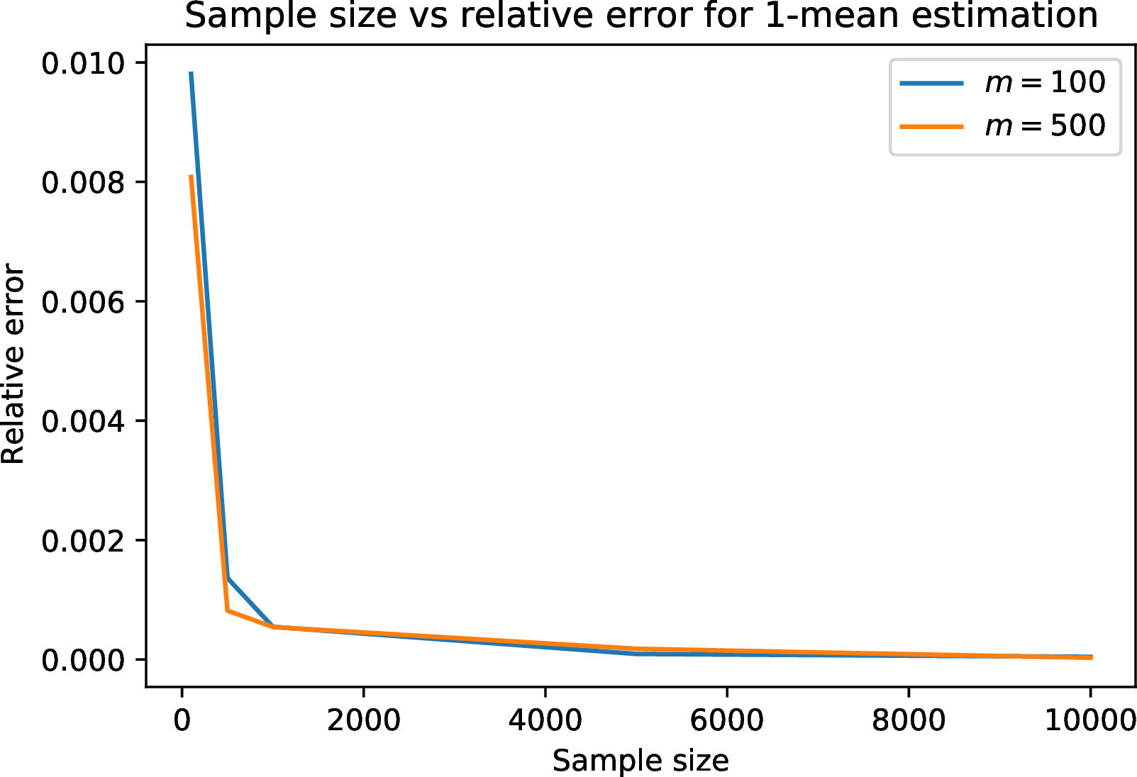
11.1 Experiment code↩︎

We provide the code snippet for the experimental evaluation below.

References↩︎